improving skip side slipper plate design to accommodate

Improving Skip Side Slipper Plate Design to Accommodate

Higher Impact Bunton Force

by

Maykel E. S. Hanna

BScE, University of New Brunswick, 2015

A Thesis submitted in Partial Fulfillment of

the Requirements for the Degree of

Master of Science in Engineering

In the Graduate Academic unit of Civil Engineering

Supervisors: Alan Lloyd, PhD, Department of Civil Engineering

Timo Tikka, PhD, PEng, Department of Civil Engineering & Stantec

Examining Board: Kaveh Arjomandi, PhD, PEng, Department of Civil Engineering

Won Taek Oh, PhD, PEng, Department of Civil Engineering

Mohsen Mohammadi, PhD, Department of Mechanical Engineering

This thesis is accepted by the Dean of Graduate Studies

THE UNIVERSITY OF NEW BRUNSWICK

September, 2017

© Maykel Hanna, 2017

ii

Abstract

This research explored new ways to improve mine conveyance side slippers

design, used to reduce the impact loads from the lateral movement resulting from

misaligned mineshaft guiding system caused during the hoisting process. The research

examined the dynamic behavior of conveyances using Comro design guideline (1990)

and compared it against single degree of freedom analysis (SDOF). A soft material,

rubber bearing pads, was added to the slipper design to reduce the total stiffness of the

system, reducing the magnitude of the lateral impact force. Cotton duck pads, a type of

bearing pad, were tested under strain rates of 0.001 to 200s-1 to investigate their behavior

under different strain rates and calculate a secant modulus of elasticity (300-400 MPa)

to be used in the final slipper design. A new slipper was designed to increase the

productivity of old and new mines. Design guidelines for the new slippers are presented

in this thesis.

iii

Acknowledgments

I hereby acknowledge and greatly appreciate the assistance of the following people and

organizations:

Dr. Alan Lloyd, for his guidance, advice and encouragement in supervising this

work and proof-reading this document.

Dr. Timo Tikka, for supervising the work and proof-reading this document.

Natural Sciences and Engineering Research Council of Canada (NSERC), for

funding the research.

Stantec Consulting Ltd., for partially funding this research and providing the

information required to conduct the research.

Fabreeka International Inc., for providing the specimens needed to conduct the

research.

The Department of Civil Engineering, University of New Brunswick, for

providing the necessary equipment for performing the tests.

iv

Table of contents

Abstract ............................................................................................................................ ii

Acknowledgments .......................................................................................................... iii

Table of contents ............................................................................................................ iv

List of Tables ................................................................................................................. vii

List of Figures ................................................................................................................. ix

1 Chapter 1 Introduction to the problem .................................................................... 1

1.1 Introduction ......................................................................................................... 1 1.2 Literature review ................................................................................................. 2

Mining loads .............................................................................................. 2 Elastomeric pads ....................................................................................... 4

Conclusion ................................................................................................ 13 1.3 Proposed research ............................................................................................. 13

2 Chapter 2 The dynamic behavior of mine shaft systems ...................................... 18 2.1 The skip dynamic behavior .............................................................................. 18

Roller-active configuration ..................................................................... 19

Inactive-rollers configuration ................................................................ 31 2.2 Computer models. ............................................................................................. 33

DISC ......................................................................................................... 34 Skip II ....................................................................................................... 41

SLAM ....................................................................................................... 42 2.3 Design procedures ............................................................................................. 44

Shaft steelwork design ............................................................................ 45 2.4 Analysis .............................................................................................................. 47 2.5 Dynamic response using Newmark β method ................................................ 49

Building the SDOF model ....................................................................... 50 Constant velocity or lumped-impulse .................................................... 51

Linear-acceleration method ................................................................... 53 Newmark β method ................................................................................. 55 Numerical integration by spreadsheet .................................................. 55

2.6 Conclusion .......................................................................................................... 61

3 Chapter 3 Experimental procedure ........................................................................ 63 3.1 Static compressive test ...................................................................................... 63

Equipment description ........................................................................... 63

Data acquisition ....................................................................................... 67 Samples preparation ............................................................................... 67 Summary of the test methodology ......................................................... 69

3.2 Impact test.......................................................................................................... 69 Summary of test method and equipment .............................................. 70

v

Data acquisition ....................................................................................... 79

Samples preparation ............................................................................... 81

Summary of the test methodology ......................................................... 82

4 Chapter 4 Experimental Results ............................................................................. 84 4.1 Static compression test results ......................................................................... 84

4.1.1 Discussion & summary ........................................................................... 87 4.1.2 Results comparison ................................................................................. 89

4.1.3 DIC results for static test ........................................................................ 91 4.1.4 Conclusion ................................................................................................ 93

4.2 Impact test results ............................................................................................. 94 Results comparison ................................................................................. 98 Multiple impact tests and failure modes ............................................. 102

Errors and recommendations to improve the test results ................. 107 Conclusion .............................................................................................. 109

4.3 Comparing static compression test results and impact test results ............ 110

5 Chapter 5 Developing a new slipper design ......................................................... 112

5.1 Current slipper plate design ........................................................................... 112 5.2 The new slipper design using the SDOF Newmark’s method ..................... 114

Calculating the maximum bunton force and displacement using EP 116

Calculating the maximum bunton force and displacement using secant

value of modulus of elasticity (E*).................................................................. 120

5.3 The new slipper design using Comro guideline ............................................ 123 5.4 Conclusion ........................................................................................................ 126

6 Chapter 6 Conclusion ............................................................................................. 128 6.1 Conclusions ...................................................................................................... 128

6.2 Suggestions for further research.................................................................... 130

References .................................................................................................................... 131

Appendix ...................................................................................................................... 133

A Example for calculating the bunton force using Comro (1990) .................. 134 A.1 General information.............................................................................. 134 A.2 Shaft steelwork design .......................................................................... 135

B Data acquisition systems ................................................................................. 141 B.1 Data acquisition system for accelerometer and load cell ................... 141

B.2 Data acquisition system for displacement ........................................... 142

C Lab reports for static testing .......................................................................... 147 C.1 Lab report 1 ........................................................................................... 148 C.2 Lab report 2 ........................................................................................... 150 C.3 Lab report 3 ........................................................................................... 152 C.4 Lab report 4 ........................................................................................... 154 C.5 Lab report 5 ........................................................................................... 156

vi

C.6 Lab report 6 ........................................................................................... 158

C.7 Lab report 7 ........................................................................................... 160

D Lab Reports for Impact Testing .................................................................... 162 D.1 Lab report 8 ........................................................................................... 163 D.2 Lab report 9 .......................................................................................... 166 D.3 Lab report 10 ........................................................................................ 169 D.4 Lab report 11 ........................................................................................ 172

D.5 Lab report 12 ........................................................................................ 175 D.6 Lab report 13 ........................................................................................ 178

CURRICULUM VITAE

vii

List of Tables

Table 2.3-1: Shaft Category, Design and Performance Parameters (Comro1990 &

SANS 10208-4). .............................................................................................................. 44

Table 3.1.3-1: Number of specimens used in every loading rate .............................. 68

Table 3.1.3-2 Loading rate and expected strain rate for each CDP thickness ........ 68

Table 3.2.3-1 Number of specimens used for each Charpy position. ....................... 82

Table 4.1-1: Dimensions, test type, and loading rate for each sample for tests 1 to 7.

......................................................................................................................................... 85

Table 4.1.2-1: Modulus elasticity calculated at 20, 45, & 70 MPa stress and strain

rate. ................................................................................................................................. 90

Table 4.2.1-1: Stress second-degree polynomial, secant modulus of elasticity

equation (E) and R². .................................................................................................... 100

Table 4.2.2-1 the thicknesses and maximum stresses for each impact test for

samples C-9 & D-9. ..................................................................................................... 103


samples C-11 & D-11. ................................................................................................. 105


samples C-13 & D-13. ................................................................................................. 106

Table 5.2-1: 𝑬𝒑 modulus of elasticity and pad stiffness 𝒌𝒑 based on secant

calculations, where u is the pad displacement and t is the pad thickness. ............. 116

Table 5.3-1: SDOF integration Spreadsheet results for bunton force, skip

displacement, pad stress & pad deflection (for skip without pad and with 6 washers

using Ep function and the equivalent E*) and the results using Comro guideline for

the same washer sizes. ................................................................................................. 126

Table C.1-1: Stresses at different specified strain for each of the four samples,

calculated based on the measured dimensions of each sample. .............................. 149



Table C.3-1 Stresses at different specified strain for each of the four samples,


viii









Table D.1-1 Stresses at different specified strain for each of the four samples

calculated based on the measured dimensions of each sample from inbound

response ........................................................................................................................ 163



response ........................................................................................................................ 166



response ........................................................................................................................ 169



response ........................................................................................................................ 172



response ........................................................................................................................ 175



response ........................................................................................................................ 178

ix

List of Figures

Figure 1.2-1 Elastomeric bearing pads (AASHTO 2012) ............................................ 6

Figure 1.2-2 Bearing Pads under compression: (a) PEP, (b) PEP with 2 surface in

contact with a structural mterial, (c) PEP under compression, (d) reinforced pad

under compression. (Stanton and Roeder 1982). ......................................................... 7

Figure 1.2-3 (a) reinforcement restrain the bulging in compression, (b)

reinforcement restrain the bulging in rotation, (c) reinforcement restrain the

bulging in shear (Roeder and Stanton 1983). ............................................................... 8

Figure 1.2-4 Relation between the International Rubber Hardness (I.R.H.) and the

elastic modulus of the natural rubber (Gent 1958). ..................................................... 9

Figure 1.2-5: Compressive stress and strain as a function of shape factor; a) CDP,

b) PEP, and c) Steel reinforced elastomeric pad (Roeder 1999). .............................. 11

Figure 1.2-6 CDPs failure states: (a) no damage, (b) oil secretion, (c) delamination,

(d) diagonal failure due to compression, (e) diagonal failure due to rotation, and (f)

internal slip (Lehman & Roeder 2005). ...................................................................... 13

Figure 1.3-1: Mineshaft Configuration - Plan View (Stantec 2013). ........................ 15

Figure 1.3-2: Slipper design and location of bearing pads ........................................ 16

Figure 2.1-1: Roller and slipper mounted on the side of the skip (COMRO 1990) 19

Figure 2.1-2: Skip model without rollers (COMRO 1990) ........................................ 20

Figure 2.1-3: Idealized guide misalignment (COMRO 1990) ................................... 21

Figure 2.1-4: Skip model without rollers (COMRO 1990) ........................................ 22

Figure 2.1-5 Guide bump and the harmonic response of the skip (COMRO 1990) 23

Figure 2.1-6: Skip travelling over a bumpy guide and its response (COMRO 1990)

......................................................................................................................................... 24

Figure 2.1-7: Skip with damping going over a bump in a guide (COMRO 1990) .. 25

Figure 2.1-8: Skip model with two rollers and the two single-degree of freedom

representing it (COMRO 1990). .................................................................................. 26

Figure 2.1-9: Effective misalignment for a general skip and guide configuration

(COMRO 1990). ............................................................................................................ 27

x

Figure 2.1-10: Example for dividing a random guide profile into multiple periodic

waves (COMRO 1990). ................................................................................................. 28

Figure 2.1-11: General misaligned two guides profile and the equivalent parallel

and gage profiles (COMRO 1990) ............................................................................... 29

Figure 2.1-12 the roller force shock spectrum at President Steyn Gold Mine,

Number 4 Shaft (COMRO 1990). ................................................................................ 30

Figure 2.1-13 Sequence of events during severe in plane slamming (Comro 1990) 32

Figure 2.2-1: Semi-continuous guide model (Krige 1983) ......................................... 36

Figure 2.2-2: Effective stiffness of the skip/guide contact (Krige 1983) ................... 36

Figure 2.2-3: Effective guide Position (Krige 1983) ................................................... 38

Figure 2.2-4: DISC Conveyance model (Krige 1983). ................................................ 39

Figure 2.2-5: Comparing the results from DISC and SKIP II (Krige 1983). .......... 42

Figure 2.2-6: Slam force diagram on different locations of the skip slipper on the

steel guide (COMRO 1990). ......................................................................................... 43

Figure 2.3-1 The Geometry of the mine skip and the location of the effective mass

(COMRO 1990) ............................................................................................................. 47

Figure 2.5-1: Single degree of freedom set up ............................................................ 50

Figure 2.5-2: Numerical Integration using constant velocity method (Biggs 1964) 51

Figure 2.5-3 Linear-acceleration approximation (Biggs 1964) ................................. 54

Figure 2.5-4 A Sample Calculation for the SDOF Spreadsheet ................................ 59

Figure 2.5-5 The bunton force harmonic response as calculated by the spreadsheet.

......................................................................................................................................... 60

Figure 2.5-6 The deflection harmonic response as calculated by the spreadsheet. . 61

Figure 3.1-1 Universal Compression Testing Machine (UCTM) .............................. 64

Figure 3.1-2 LVDTs and Experimental set up ........................................................... 65

Figure 3.1-3 LVDTs calibration using a military height gauge ................................ 65

Figure 3.1-4 High-speed camera and light source. ..................................................... 66

Figure 3.1-5 Three specimen sizes: 12.7, 25.4, and 50.8 mm ..................................... 67

xi

Figure 3.2-1 The hammer and plate arrangement for impact measurement. ......... 71

Figure 3.2-2 Support design: (a) Spherical washers. (b) the washer, bolt, and first

steel plate. (c) The hole in the steel plate so the bolt could be easily mounted on the

steel frame. (d) Two steel plates surface ground to reduce friction between the

plates. (e) Eight bolts to connect the two plates together. (f) Final look for the

support and the space needed for the load cell and adjusting steel washers. .......... 73

Figure 3.2-3 Modified Charpy, Impact Testing Machine. ......................................... 74

Figure 3.2-4 Two pendulum hammer positions for the Charpy machine. ............... 75

Figure 3.2-5 One Dimension Shock Accelerometer. .................................................. 76

Figure 3.2-6 Wheatstone Full Bridge compression configuration (NI 2016). .......... 76

Figure 3.2-7 Customized Full Bridge Load Cell. ........................................................ 77

Figure 3.2-8 Overall set up for accelerometer and load cell in modified Charpy

testing machine. ............................................................................................................. 78

Figure 3.2-9: Two washers with thicknesses 25 mm and 37.5 mm. .......................... 79

Figure 3.2-10 NI cDAQ-9172 model and both NI9205 and NI9237 Cards. ............. 80

Figure 3.2-11 Random speckled surface. .................................................................... 81

Figure 3.2-12 CDP pattern before speckling. ............................................................. 82

Figure 3.2.4-1 Strain rates from 2 LVDT and their average for sample A-1 .......... 86

Figure 3.2.4-2: Strain rates from 2 LVDT and their average for sample A-1 ......... 86

Figure 3.2.4-3: The Stress-strain curves of the four samples tested under

12mm/min loading rate and their average (S-1-Average) ......................................... 87

Figure 4.1.1-1 Failure modes for 2 samples ................................................................ 89

Figure 4.1.2-1: Average Stress-strain curves compared for the 7 static compressive

tests. ................................................................................................................................ 90

Figure 4.1.2-2: The modulus of elasticity E values for the static test for each strain

rate calculated at stresses 20, 45, & 70 MPa. .............................................................. 91

Figure 4.1.3-1: Comparison between the displacement data calculated from DIC

analysis and the displacement data obtained from the LVDTs for sample A-7. ..... 92

Figure 4.1.3-2: The images captured by the camera to perform the DIC analysis for

Sample A-7. .................................................................................................................... 93

xii

Figure 4.1.3-1Stress-time plot for sample A-8 (including accelerometer data, load

cell data, and a noise removed plot for accelerometer data) ..................................... 96

Figure 4.1.3-2 Strain-time plot for sample A-8. ......................................................... 96

Figure 4.1.3-3 The Stress-Strain curves of the four samples tested under impact

(first hammer position) and their average (S-8-Average) ......................................... 97

Figure 4.2.1-1: Stress-strain curves compiled for the 8 sets of impact test. ............. 99

Figure 4.2.1-2: Second-degree polynomial regression of stress-strain data for tests 8

to 13. ............................................................................................................................... 99

Figure 4.2.1-3 The modulus of elasticity E values for the static test for each strain

rate calculated at stresses (20, 45, 70, & 100). .......................................................... 101

Figure 4.2.2-1 Failure modes for samples C-9 & D-9. ............................................. 103

Figure 4.2.2-2 Failure modes for samples C-11, & D-11. ........................................ 104

Figure 4.2.3-1 Example of recoverable accelerometer data noise. ......................... 107

Figure 4.2.3-2 Example of irrecoverable accelerometer data noise (high frequency

and baseline shift error).............................................................................................. 108

Figure 4.2.3-3 Multiple impact events in a single impact test. ................................ 108

Figure 5.1-1: Application of lateral loads (COMMENTARY ON SANS 10208:3 –

2001) ............................................................................................................................. 113

Figure 5.1-2: Slipper plates design (COMMENTARY ON SANS 10208:3 – 2001)

....................................................................................................................................... 113

Figure 5.2-1: The addition of the elastomer pad stiffness to the SDOF system

presented in chapter 2 to form a new SDOF system. ............................................... 114

Figure 5.2-2: CDP mounted between the slipper plate and the skip (Pad and

washer forms). ............................................................................................................. 118

Figure 5.2-3 Ratio between the bunton forces before and after adding CDP

compared by different pad thicknesses with the same area (821mm2). ................. 119

Figure 5.2-4 Ratio between the bunton forces before and after adding CDP

compared by different pad areas with the same pad thickness (50.8 mm). ........... 120

Figure 5.2-5: Actual stress-strain curve of CDP and the curves created by the

equivalent values of E* for 20 MPa allowable stress. .............................................. 122

xiii

Figure 5.2-6 Actual stress-strain curve of CDP and the curves created by the

equivalent values of E* for 35 MPa allowable stress. .............................................. 122

Figure 5.3-1: Flowchart for the new slipper design. ................................................ 125

Figure A.1-1 Mineshaft plan view configuration ..................................................... 135

Figure A.2-1:Contour plot of rebound velocity ratio ru (Comro 1990). ................. 137

Figure A.2-2: Contour plot of nondimensional bunton force 𝑷𝒃 for u/v = 0.005

(Comro 1990). .............................................................................................................. 138

Figure A.2-3: Contour plot of nondimentional skip displacement 𝜹𝒔 for u/v = 0.005

(Comro 1990). .............................................................................................................. 139

Figure A.2-4: Contour plot of nondimentional guide bending moment 𝑴 for u/v

=0.005 (Comro 1990). .................................................................................................. 140

Figure B.2-1: Photron FastCam viewer ver 2 used to record the high-speed

camera’s images. ......................................................................................................... 142

Figure B.2-2: The reference image and the impact event images. .......................... 143

Figure B.2-3: Drawing region of interest .................................................................. 144

Figure B.2-4: Identifying the unit conversion factor ............................................... 145

Figure B.2-5: Matlab Array of pixel displacements for image 23. ......................... 146

Figure C.1-1: Specimen Dimensions .......................................................................... 148

Figure C.1-2: (UCTM) set up. .................................................................................... 148

Figure C.1-3: Strain rates from 2 LVDT and their average for sample A-1 ......... 148

Figure C.1-4: Stress-strain curves for 2 LVDTs and their average for sample A-1

....................................................................................................................................... 148

Figure C.1-5: The Stress-strain curves of the four samples tested under 12mm/min

loading rate and their average (S-1-Average) .......................................................... 149





....................................................................................................................................... 150

xiv







....................................................................................................................................... 152






Figure C.4-4: The Stress-strain curves of the four samples tested under

400mm/min loading rate and their average (S-4-Average) ..................................... 155

Figure C.5-1 Specimen dimensions ............................................................................ 156




....................................................................................................................................... 156

Figure C.5-5: The Stress-strain curves of the four samples tested under

160mm/min loading rate and their average (S-5-Average) ..................................... 157

Figure C.6-1 Specimen dimensions ............................................................................ 158


Figure D.1-1: Specimen Dimensions .......................................................................... 163

Figure D.1-2: MCIM set up. ....................................................................................... 163

Figure D.1-3: Stress-Time plot for sample A-8 (including accelerometer data, load

cell data, and a noise removed plot for accelerometer data) ................................... 164

Figure D.1-4: Strain-Time plot for sample A-8 and images acquired from the high-

speed camera for DIC analysis................................................................................... 164

xv

Figure D.1-5: The Stress-Strain curves of the four samples tested under impact

(first hammer position) and their average (S-8-Average) ....................................... 165





Figure D.2-4: Strain-Time plot for sample A-9 and image acquired by the high-



(first hammer position) and their average (S-9-Average) ....................................... 168





Figure D.3-4: Strain-Time plot for sample A-10 and images acquired by the high-



(first hammer position) and their average (S-10-Average) ..................................... 171







Figure D.4-5: The Stress-Strain curves of the three samples tested under impact

(second hammer position) and their average (S-11-Average) ................................. 174





xvi













1

1 Chapter 1 Introduction to the problem

Introduction

Mining components are some of the most complex structures in the building field.

Mineshafts are among the most important components of the infrastructure in deep mines

as they are used for transporting people and materials to and from the mine core as well

as lifting the raw materials to the surface. A steel system (steelwork) is used to divide the

mineshaft area and provide guidance to the movement of conveyances between the

surface and the mine core. This steelwork is comprised of horizontal buntons and vertical

guides. The horizontal buntons are used to support the guides and transfer the loads of the

hoisting process to the supports on the mineshaft walls. The guides are used to guide the

vertical movement, while limiting the lateral movements, of the conveyances. This

research focuses on the dynamic system where two guides guide the vertical movement

(hoisting) of each conveyance. The guides are located on opposite sides of the

conveyances. The steel guides and buntons are susceptible to multiple damaging

mechanisms including fatigue damage, plastic deformation of conveyances and guide

derails. Impact forces on these components are expected to reach 2 to 3 times the gravity

load of the conveyance in the form of horizontal impact (Krige 1983). In other words, the

magnitude of impact forces can reach 2 to 3 times the weight of the loaded conveyances,

which can be in excess of one hundred tons.

Problem statement:

The demand on mine conveyances is increasing as material is being transported to

the surface in larger quantities than ever. Mines require higher mass conveyances moving

2

with higher hoisting speeds. Both contribute to potentially higher lateral impact forces

(slam loads) from the conveyance onto the guide system. The magnitude of these slam

loads needs to be reduced to mitigate potential damage to the guide rail system and allow

continuous operation of mines.

Literature review

This section and Chapter 2 present an extensive background study of previous

research investigating the topics of this thesis. It starts by explaining different mine shaft

loads and the need for adding a rubber pad to reduce the impact load effect at the slipper

location. Furthermore, it discusses a detailed study of elastomeric pad design as specified

by the bridge AASHTO standards (2012).

Mining loads

A subsurface mine is generally divided into three components: Surface structures,

a mineshaft, and a mine core. Surface structures organize the movement of conveyances

hoisting people and materials from the mine core to the surface passing through the

mineshaft. The mineshaft is the vertical tunnel connecting the surface to the mine core.

The mineshaft is usually divided into multiple compartments. These compartments permit

conveyances to move easily to transport people and materials from the mine to the surface.

Each compartment contains at least two guides to guide a conveyance’s movement. These

guides are supported by buntons anchored to the walls of the mineshaft. The buntons and

guides are considered the steelwork of the mineshaft carrying the loads exercised by the

hoisting process. The mine core is the active mine area where raw materials are extracted.

3

This research is only considering the loads exercised on the steel shaft system, guides and

buntons, by the conveyances traveling between the surface and the core.

Permanent loads

South African National Standard, Design of structures for the mining industry

SANS 10208-4 (2011) is a design code used in the mining industry worldwide. This

design code divides the permanent load into:

Self-weight of the steel work of the mineshaft.

Rocks loads on the sides of a mineshaft supported by brow beam and sidewalls.

Conveyor operating loads.

These loads are important in steelwork design but are not part of this research interest.

Dynamic loads

During the last few decades, researchers studied multiple mines to calculate the

maximum bunton forces and deflections using load cells, strain gauges and computer

programs (Krige 1986). The results of these investigations were compiled into a complete

guideline to design mineshafts subjected to slam loads (Comro 1990). This guideline was

also incorporated into the SANS 10208-4 (2011). In most cases of slam events, the rollers,

located on the top of the skip, reduce the impact force exercised by the skip on the

steelwork of the mine shaft. Over time, the rollers wear out and become inactive. In turn,

the steel slippers mounted on both sides of the skip slam the steel guides directly without

dissipating the force causing larger forces on the steelwork. These steel slippers are

usually covered with a high-density polyethylene (HDPE) layer to reduce friction between

4

the slipper plate and the guide. Therefore, understanding the dynamic response of skip

with inactive rollers is critical.

To calculate the magnitude of the forces on buntons and deflections of buntons,

Comro (1990) transform the skip and the steel work system into a single degree of

freedom system. This single degree of freedom system is formed using an effective mass

of the conveyance computed about the impact location of the slipper at the leading end of

the skip. The system also uses two springs in series representing the skip stiffness and the

bunton stiffness. If the skip is very stiff, the total stiffness is considered to be only the

bunton stiffness. Finally, the system has an initial velocity equal to impact velocity. This

system will be discussed in detail in Chapter 2.

Elastomeric pads

To reduce the slamming force, a new slipper design could be developed using a

combination of rubber type material and steel. The rubber material will reduce the

effective stiffness of the system which in turn reduces the slamming force on the steel

buntons. It will also play an important role for dissipating the dynamic behavior of the

steel shaft. The hyper-elasticity of rubber is a useful property for damping dynamic loads.

Rubber bearing pads have been used for multiple such applications including mitigating

seismic loads and traffic loads on bridges (Roeder and Stanton 1983). Four types of rubber

pads are specified in the American Association of State Highway and Transportation

Officials (AASHTO): plain unreinforced elastomeric pads (PEP), Fiberglass-Reinforced

Pad (FGR), Steel-Reinforced Elastomeric Bearing, and Cotton-Duck-Reinforced Pad

(CDP).

5

To reduce the extreme impact loads, the new slipper design should provide a

reasonable amount of load reduction, accommodate movement, and prevent premature

fatigue failures or creep failures. As slippers are mounted on the sides of conveyances,

the new design should have a rectangular shape to accommodate for the clearance between

the guide and the slipper. Rubber bearing pads were found to be a realistic solution in this

case for their capability in seismic base isolation and machine vibration control (Roeder

and Stanton 1983) and their high allowable compressive capacity which can reach 20 MPa

for fatigue loads (AASHTO 2012).

Roeder and Stanton (1983) provided a summary for different types of bearing pads

and the gap between structural design and the manufacturers points of view of the

elastomers bearing pads. They demonstrated two main types of rubber materials used in

elastomeric pads: natural rubber or a synthetic rubber such as chloroprene. These rubber

materials have a nonlinear stress-strain behavior affected by both temperature and strain

rate. In general, the rubber pads stiffen under low temperatures and high strain rates.

Manufacturing of elastomeric pads

Raw rubber is a soft material with a very low stiffness. To resist higher stress with

small deflection, the raw rubber should be reinforced by layers of reinforcements then

vulcanized after bonding the reinforcement to the rubber (Roeder and Stanton 1983). This

method secures a strong bond between the rubber and the reinforcement. During this

procedure, some antiozonants, antioxidants, and fillers like oil and carbon black are

added. These compounds affect the mechanical behavior of the rubber. The properties of

the rubber can change from one manufacture to another, challenging structural engineers

to design bearing pads (Roeder 2000). The structural engineer focuses mainly on the

6

mechanical properties of rubber pads including stiffness, strength and stress- strain

relation of the bearing pad. On the other hand, the manufacturers’ focus is limited to

achieve a certain range of hardness and elongation break (Roeder and Stanton 1983).

Figure 1.2-1 shows an example of a rubber bearing pad.

CDPs are manufactured under the military specification MIL-C-882-E (1989).

CDP consists of thin layers of elastomer and cotton duck fabric. Generally, CDP is stiffer

and has higher compressive strength than other pad types (Roeder 2000).

Different types of elastomeric pads

Elastomeric pads are generally classified by the type of the reinforcement used

between the rubber layers. Four types of elastomeric pad specified in the AASHTO LRFD

Design Specifications (2012) are; PEP, FGR, Steel-Reinforced Elastomeric Bearing, and

CDP.

PEP is a plain rubber pad without any reinforcement layers. It is considered the

least stiffened rubber pad in all the elastomeric pads. As the pad is formed completely

Figure 1.2-1 Elastomeric bearing pads (AASHTO 2012)

7

from rubber, the only force restraining the bulge of the pad is the friction between the

rubber surface and the surface of the contacting material. This friction force depends on

the type of material it is in contact with. The design of this type of pad is not permitted in

some building codes and is penalized by others by reducing the effective mechanical

properties used in design. (Roeder and Stanton 1983).

A steel reinforced bearing pad is formed of natural rubber or synthetic rubber with

steel layers. The steel provides the pad increased in-plane stiffness by reducing the

bulging area which reduces the total bulging of the pad (see Figure 1.2-2). The steel

reinforcements restrain the pad’s lateral deflection, bulging, which increases compressive,

shear, and rotation capacity (see Figure 1.2-3). In a reinforced pad, the shear stress in the

pad transforms into a tensile stress in the reinforcement layers. As steel has high tensile

capacity, few complications happened due to this tensile stress (Stanton and Roeder

1982).

Figure 1.2-2 Bearing Pads under compression: (a) PEP, (b) PEP with 2 surface in contact

with a structural mterial, (c) PEP under compression, (d) reinforced pad under

compression. (Stanton and Roeder 1982).

8

Fiberglass was used as reinforcing material in elastomeric pads. Fiberglass is

much weaker than steel in tension which permit a better control of the strength of the

bearing pad (Roeder and Stanton 1983).

Cotton duck pads (CDP) are produced in form of cotton duck material sheets,

specified in the Military Specification MIL-C-882-E (1989), interlayered by layers of

elastomer. Polytetrafluorethylene (PTFE) is used on the top of the pad as a sliding surface

which accommodate for pad translation. CDP are known for their high stiffness relative

to other bearing pad types. The hardness of this type of pad could reach 90 on a durometer

shore A scale. High stiffness and hardness provide CDP with a higher compressive

capacity and strength. Nevertheless, the thin layers of cotton duck deliver a higher

rotational and shear stiffness which leads to a higher moments and edge capacities. These

Figure 1.2-3 (a) reinforcement restrain the bulging in compression, (b) reinforcement

restrain the bulging in rotation, (c) reinforcement restrain the bulging in shear (Roeder and

Stanton 1983).

9

higher rotational and shear stiffness also reduce the total shear and rotational deflections

of the pads (Roeder 1999).

Rubber pad properties and design criteria

Hardness

Gent (1958) studied the relation between the hardness of natural rubber and

modulus of elasticity. Gent derived a graph to describe this relation using the international

rubber hardness (IRH) degrees and formulated in terms of deformation theory. This

formula was compared with multiple experiments on natural rubber specimens (see Figure

1.2-4). The range of interest for the rubber hardness is between 50 and 70 Shore A

hardness test.

Figure 1.2-4 Relation between the International Rubber Hardness

(I.R.H.) and the elastic modulus of the natural rubber (Gent 1958).

10

Compression

AASHTO (2012) limits the compressive stress of PEP to 0.8 ksi (5.5 MPa), FGP

to 1 ksi (6.87 MPa), steel reinforced pad to 1.25ksi (8.58 MPa) and CDP to 3 ksi (20.6

MPa). AASHTO describes the stress in PEP and FGP using the pad shape factor and the

shear modulus. The shape factor of a pad is the ratio between the pad area and its perimeter

area. Due to CDP manufacture procedures, the shape factor of CDP has a smaller effect

on the behavior of the CDP compared to other pad types. Roeder (1999) compared the

compressive behavior of CDP and the other pad types. CDP was found to have a higher

stiffness and higher compressive strength. PEP had the lowest stiffness as it does not

contain any reinforcements. Figure 1.2-5 shows the stress-strain curves for PEP, CDP,

and steel reinforced elastomeric bearing pad.

As presented in Figure 1.2-5, the shape factor has a significant effect on both PEP

and steel reinforced elastomeric pad. On the other hand, CDP experienced less effect on

its compressive behavior compared to PEP and steel reinforced pads. In this research, the

pad designed for the slipper plate has a high shape factor (5.4), as the pad’s area is very

large, the same size as the slipper plate (200mm × 500mm), and the thickness of the pad

is very small due to limited distance between the skip and the guide. The high shape factor

increases the stiffness of PEP and steel reinforced bearing pads. Therefore, the research

focused on testing CDP where the shape factor has smaller effect on the pad properties

than PEP and steel reinforced pads. CDP was also selected due to higher compressive

allowable stress (20.6 MPa) which will be essential while designing extreme impact cases.

11

Figure 1.2-5: Compressive stress and strain as a function of shape factor; a) CDP, b) PEP,

and c) Steel reinforced elastomeric pad (Roeder 1999).

Dynamic and fatigue

Lehman and Roeder (2005) presented the results of dynamic and fatigue

compression tests for CDP samples. Their tests were designed for traffic loads. The test

was conducted using 2 million cycles of stress levels equivalent to the heaviest truck loads

with a loading rate of 1.5 Hz to avoid heat built up. This test evaluated the durability of

the material for 50 to 100 years required for bridge life design. Two types of damage were

observed: delamination of the cotton duck layer and oil secretion. The damage category

12

will be discussed in the following section. For samples tested to stress up to 7 MPa, the

damage was limited to oil secretion. For samples tested for maximum stresses of 14-21

MPa, the damage reached delamination of the cotton duck layers. The maximum stress

range had the most significant effect on the behavior and failure of the CDPs. To

maximize the pad durability, they recommended stress limit of 3 ksi (20.6 MPa).

Pads modes of failure

Lehman & Roeder (2005) categorized the test damage states of the CDP into 5

categories (see Figure 1.2-6):

No damage (Figure 1.2-6(a))

Secretion of oil or wax (Figure 1.2-6(b))

Delamination of CDP Layer (Figure 1.2-6(c)).

Fracture or cracking (Figure 1.2-6(d & e)).

Internal split (Figure 1.2-6(f)).

Pads that were subjected to limited maximum strain or stress showed no damage. Oil

secretion from the pad occurred during long-term compression tests including the

dynamic compression tests with minimum stress of 7 MPa. For these first two categories,

CDPs were still functional. Pads, that were subjected to dynamic and uplift tests, showed

delamination of cotton duck layers. Diagonal failures were present due to high stress

compression or rotation tests. The last category, internal split, was observed in shear tests

with large shear deformations. Bearings that exhibited fractures or internal split damages

are required to be immediate replaced in the field.

13

Figure 1.2-6 CDPs failure states: (a) no damage, (b) oil secretion, (c) delamination, (d)

diagonal failure due to compression, (e) diagonal failure due to rotation, and (f) internal

slip (Lehman & Roeder 2005).

Conclusion

The previous CDP research focused on the compression and fatigue testing which

describes the material behavior and compare it with other bearing pad types. This research

will focus on the behavior of CDP under high impact loads. Examining this impact

behavior will provide the information needed to design a flexible slipper to be mounted

on the mine skip to reduce the dynamic behavior of the skip/guide system which will

reduce the magnitude of impact load in the mineshaft.

Proposed research

The objectives of this study are as follows:

14

1. To assess the industry standard methodology of determining slam loads.

2. To determine an appropriate interface material that can be placed between mine

skip slippers and rails to potentially reduce force transfer and mitigate slam

loads.

3. To experimentally validate the static material properties of the interface material

to ensure its appropriateness for use in the slipper design.

4. To experimentally determine the high strain rate behavior of the material to

incorporate its dynamic material properties into the slipper design.

5. To simplify the material response into elastic equivalent single degree of

freedom and equivalent static force procedure models for practical use in design

of slippers.

6. To propose a simple design procedure for incorporating the interface material

into slipper design.

The proposed research will consider a potash mineshaft located in Saskatchewan,

Canada. The typical mineshaft configuration consists of two skips for material hoisting

(A1, A2), a cage for people and equipment transportation to the mine location

underground (C1), and a counter weight to balance the movement of the cage (B1) (see

Figure 1.3-1).

15

An analysis of the mineshaft steelwork will be carried out to define the lateral

loads developed in the steelwork as a result of the dynamic interaction between the

conveyances and the conveyance guiding system. The dynamic interaction between

conveyances and the shaft steelwork depends on multiple factors. These factors include

the misalignment of the shaft guide, the bunton, skip, and guide stiffnesses, the mass of

the skip, and the hoisting velocity. After analyzing the impact force, a bearing pad will

be considered to reduce the impact force. This bearing pad will consist of a rubber-like

material with low stiffness to change the dynamic response of the system and reduce the

impact force at bunton location. In this mineshaft, a bearing pad is located originally on

the slippers located on the sides of the conveyances (see Figure 1.3-2). An optimized

design of the bearing pad will be explored with pad properties selected to reduce slam

loads from the conveyance onto the rail system.

A1

1

A2

B1

C1

Figure 1.3-1: Mineshaft Configuration - Plan View (Stantec 2013).

Guides

Buntons

16

Unlike traditional bearing pads, the rubber, in this case, will not carry large gravity

loads. The rubber will carry dynamic loads including cyclic and extreme rare impact

loads. Cotton duck pads (CDP) will be used in this research at the slipper location. Due

to the lack of information on the dynamic behavior and properties of CDP, CDP samples

will be tested under static and dynamic loadings. This research will present a full design

guideline for design bearing pads used to prevent rare and extreme impact loads in a

mineshaft.

After the introductory information and literature review presented in this chapter,

the thesis structure is as follows:

Chapter 2 presents the dynamic properties of mine shaft systems and discusses

dynamic analysis procedures.

Guide

Bearing

pads

Slipper

Conveyance

Figure 1.3-2: Slipper design and location of bearing pads

17

Chapter 3 describes the experimental procedure that was employed to test the

static and dynamic material properties of the material added to the slipper to

interface with mine shaft rails.

Chapter 4 presents the experimental results of the procedure outlined in Chapter

3. The influence of different parameters is explored along with response of

materials under different strain rates. Supplementary data from the experimental

results is presented in Appendix C and Appendix D.

Chapter 5 describes the proposed methods to incorporate the interface material

into slipper design to reduce slam loads.

Chapter 6 presents conclusions and suggestions for future research that stem from

this work.

In addition to the above chapters, there are four appendices that present an

example calculation of slam loads (Appendix A), the data acquisition system and

experimental test monitoring process (Appendix B), and experimental data summaries

from the static tests (Appendix C) and the dynamic tests (Appendix D).

18

2 Chapter 2 The dynamic behavior of mine shaft systems

This chapter illustrates an overview of the theoretical aspects of designing a shaft

steelwork/skip system for dynamic loads. The chapter contains a summary of how the

COMRO (1990) guideline have been completed though the last few years. The chapter is

divided into multiple parts:

Understanding the skip behavior in both active and inactive rollers scenarios.

Comparing different commercial software used to analyze the dynamic

behavior of the skip and mineshaft steelwork.

Using Comro (1990) guideline to calculate the impact bunton force and

maximum guide deflection.

Developing a spreadsheet to calculate the maximum impact force and guide

deflection of the approximated single degree of freedom system (SDOF) and

compare its results to the guideline results.

After explaining the details of developing and understanding the dynamic behavior of

the skip/steelwork system, the results will be used in designing the cotton duck pad (CDP)

attached to the skip slippers. The new design takes into consideration the data gathered in

the experimental results discussed in Chapter 4.

The skip dynamic behavior

This part describes the dynamic behavior of skips and shaft steelwork as described in

Comro (1990). The skip-guide behavior is divided into two associated parts. The first is

considering the rollers on the sides of the skip are fully effective. The second is

19

Figure 2.1-1: Roller and slipper mounted on the

side of the skip (COMRO 1990)

considering the rollers are not active and the impact occurs on the slippers mounted on

both sides of the skip. In a real situation, both scenarios occur at the same time. The roller

located at the top or the bottom of the skip start by deflecting until it is no longer active

and the slipper on the side of the skip impact the guide causing the most harming effect

on the mineshaft steelwork (see Figure 2.1-1). To simplify the analysis, Comro guideline

provided some dynamic fundamentals to describe the theory behind the dynamic behavior

of the skip/guide system.

Roller-active configuration

Comro provided a study that can be used by readers to understand the dynamic

behavior of skip/guide system in case of active-roller. This study is divided into five

Roller Configuration

Slipper

20

Figure 2.1-2: Skip model without rollers (COMRO 1990)

systems starting from the simplest dynamic model and adding more complications in form

of variables to reach a more realistic model.

System 1

This system considers the total mass of the skip as a dimensionless mass (ms). This

mass is traveling along a rigid guide without roller isolating the guide misalignment (see

Figure 2.1-2). As the mass is translating with a constant velocity, the lateral acceleration

is calculated using the following equation:

𝑑2𝑥

𝑑𝑡2 = 𝑑2𝑥

𝑑𝑦2 (𝑑𝑦

𝑑𝑡)

2= 𝑑

2𝑥

𝑑𝑦2 v2 Equation 2-1

where x is the skip’s lateral displacement and y is the vertical displacement.

The force acting the guide, caused by the lateral movement of the skip is expressed

as:

21

Figure 2.1-3: Idealized guide misalignment (COMRO 1990)

Force= mass* acceleration

= ms v2

𝑑2𝑥

𝑑𝑦2 Equation 2-2

This equation illustrates that the acting force of the skip on the steelwork is quadratic

related to the hoisting speed, the skip vertical speed. In other words, if the velocity of the

skip increases, it will increase the impact force.

To evaluate the peak value of acceleration, a uniform cosine wave misalignment

was selected to prevent the typical shaft peak misalignment (see Figure 2.1-3).

For a peak to peak amplitude of 30 mm, the maximum curvature is calculated as

follows:

22

Figure 2.1-4: Skip model without rollers (COMRO 1990)

x = 15 cos 𝑦𝜋

2500 =

𝑑2𝑥

𝑑𝑦2 =

15𝜋2

25002 cos

𝑦𝜋

2500 Equation 2-3

For hoisting speed equal to 15 m/s, the lateral acceleration of the skip could reach

0.5 g which result in a high impact force on the guide. Due to this high lateral force, rollers

are mounted on sides of the skip. The following section will consider the rollers effect on

system 1.

System 2

This system consists of skip mass, rigid misaligned guide, and roller represented

in a linear elastic spring between the skip mass and the guide (see Figure 2-4).

For this system, the guide misalignment profile is considered a bump in the form

of a short duration misalignment with large amplitude to produce a harmonic vibration

for the skip mass. The frequency of the system (fs) could be calculated by:

23

Figure 2.1-5 Guide bump and the harmonic response of the skip (COMRO 1990)

fs = 1

2𝜋 √

𝑘𝑟

𝑚𝑠 Equation 2-4

where kr is the roller stiffness. The initial lateral velocity is equal to the integral of the

acceleration forming the harmonic behavior of the system (see Figure 2.1-5).

If the skip is exposed to multiple bumps (see Figure 2.1-6), the vibration will build

up forming a higher amplitude. The amplitude of the skip vibration is depending on the

amplitude of the guide misalignment as described in the following equation:

𝐴𝑚= 𝛽2

(1−𝛽2) x𝐴𝑔𝑚. Equation 2-5

where 𝛽= 𝑓𝑔

𝑓𝑠 , 𝑓𝑔 is the frequency of guide excitation, Am is the amplitude of relative

motion, and Agm is the amplitude of the guide misalignment.

The system can reach resonance if the natural frequency of the system and

excitation frequency are equal. When resonance occurs, the roller load increases without

bound. To prevent this resonance situation, 𝛽 should be maintained less or more than one

to reduce the dynamic response of the skip. The case of 𝛽<<1 corresponds a small skip

24

Figure 2.1-6: Skip travelling over a bumpy guide and its response (COMRO 1990)

travelling slowly on stiff rollers over a guide with long misalignment waves. On the other

hand, 𝛽>>1 corresponds to a heavy skip on flexible rollers, high skip speed and short

wavelength misalignment. Each of these approaches are considered in the design of

shaft/steelwork, each has its own limitations.

System 3

The mineshaft steel structure normally dissipates the vibration effect; this

dissipation is called damping (see Figure 2.1-7). The amplitude of the harmonic response

of the skip should decrease over time. The amplitude equation (Equation 2-6) could be

transformed to the following equation:

𝐴r𝑚= 𝛽2

√(1−𝛽2)2+(2𝛽𝜉)2 × 𝐴g𝑚 Equation 2-6

Where Armis the amplitude of relative motion, 𝜉 is damping ratio, the ratio between rollers

damping properties and critical damping. Critical damping is defined as the situation

25

Figure 2.1-7: Skip with damping going over a bump in a guide (COMRO 1990)

where the vibration damps out without crossing zero displacement. Critical damping (𝐶𝑐)

is calculated by:

𝐶𝑐 = 2√𝑘𝑟𝑚𝑠 Equation 2-7

At resonance, the dynamic amplification factor is calculated by:

Dynamic Amplification = 1

2𝜉 Equation 2-8

For a regular roller, the damping ratio ranges between 2% and 5%. The dynamic

amplification factor is multiplied by the acceleration calculated in the system can reach

up to 12.5g.

In fact, this enormous load does not happen in real situations. In systems 1, 2, and

3, the skip is modeled as a concentrated mass with a roller on one guide. These

assumptions could be improved by assuming a skip length and two active rollers.

26

Figure 2.1-8: Skip model with two rollers and the two single-degree

of freedom representing it (COMRO 1990).

System 4

In this system, the length of the skip and rollers on both top and bottom will be

taken into consideration. The system is considered to be two degrees of freedom system.

The two degrees are then divided into two single degrees of freedom (SDOF) systems

(see Figure 2.1-8). The first system is similar to system 3 model describing the lateral

movement of the skip. The second describes the rotational behavior of the skip.

The two SDOF systems could happen separately. The translational behavior

happens when the guide misalignment wavelength is equal to the skip height. The second

is the rotational behavior of the skip which happens when the skip height is equal to one

and half times the wavelength of guide misalignment. The effect translational

misalignment could be calculated as the average of the misalignment at the two rollers.

27

Also, the rotational misalignment is the ratio between the difference in guide

misalignment at the two rollers and the skip height as shown in Figure 2.1-9.

The rotational degree of freedom could be calculated using the following terms:

The mass moment of inertia about the center of gravity (c.g.):

I = 𝑚𝑠 𝐻2

12 Equation 2-9

This formula assumes the mass is uniformly distributed along its length H, which is much

longer than the width of the skip. The rotational stiffness when 2 rollers are in contact

with guide:

Figure 2.1-9: Effective misalignment for a general skip and guide configuration

(COMRO 1990).

28

Figure 2.1-10: Example for dividing a random guide profile

into multiple periodic waves (COMRO 1990).

𝑘𝜃 = 2 𝑘𝑟 (𝐻

2)

2

= 1

2 𝑘𝑟 𝐻2 Equation 2-10

This formula assumes that the rollers are symmetrically placed with respect to the skip

c.g. If the c.g. of the skip is not symmetrically placed, it is advised using a computer model

to calculate the mass moment of the inertia and the rotational stiffness.

The guide misalignment profile is not usually in a waveform. This profile could

be solved by using superposition of multiple waves (see Figure 2.1-10). The skip’s

dynamic response for each of these waves could be solved separately and the results will

be combined to form the expected dynamic response of the skip. This system is used in

guidelines are based for the rollers-active case.

29

Figure 2.1-11: General misaligned two guides profile and the

equivalent parallel and gage profiles (COMRO 1990)

Computer programs could be used to evaluate the dynamic response of the skip

for each waveform and combine them to get the overall dynamic response of the skip.

Up to system 4, the dynamic behavior discussed was composed of a skip, a guide,

and maximum of two rollers. The following system will discuss the dynamic behavior of

the skip while considering two guides, one on each side of the skip.

System 5

This system contains the description of the skip system with two guides, one guide

on each side profile and how this profile affects the behavior of the skip. Figure 2.1-11

shows two misaligned guides profile which could be divided into parallel misaligned

guides and a gage profile.

The gage variation was found not affecting the vibration of the system along with

the analysis procedures of the dynamic behavior of the guide/skip system. On the other

hand, the gage profile will affect the static force of the skip roller directly. This change of

30

Figure 2.1-12 the roller force shock spectrum at President Steyn Gold

Mine, Number 4 Shaft (COMRO 1990).

roller force should be taken into consideration while designing the steelwork of the

mineshaft.

The presence of a second guide will not affect the analytical complexity of the

system. It is safe to assume that minimum of two rollers will be active with a preload on

the guides. But, for design purposes, it is advised performing the analysis twice: once with

only two active rollers and the second has four active rollers.

To develop a plot describing the peak dynamic response for the shaft, it is

necessary to perform many dynamic simulations, each with a different skip natural

frequency and damping values. This plot could be used to determine the roller force

related to the unit mass of the skip. Figure 2.1-12 shows an example of the roller force

shock spectrum at President Steyn Gold Mine, Number 4 Shaft.

Half bunton

passing frequency

0.020

0.050

0.120

0.150

0.220

0.250

0.320

0.350

0.00 0.25 0.50 0.75 1.00 1.25 1.50 1.75 2.00 2.25 2.50 2.75 3.00

Roll

er F

orc

e (N

/kg)

Skip Frequency (Hz)

31

This spectrum is commonly used to present the dynamic response of multiple

shock and vibration in different industries.

As a conclusion, the roller’s low stiffness is considered the main reason for

reducing the guide misalignment effect on the skip bouncing behavior. In the case of

rollers failure or excess deflection, the slippers on both sides of the skip impact directly

on the guides. Overall, to reduce the roller force, the designer could use, as discussed in

system 2, one of two scenarios a small skip traveling slowly on stiff rollers over a guide

with long misalignment waves or a heavy skip on flexible rollers, high skip speed, and

short wavelength misalignment. Scenario 2 is more likely the situation in the mining

operations.

Inactive-rollers configuration

In this model, the rollers mounted on the skip are considered not active. The

slipper on the side of the skip impacts the mineshaft’s steelwork making the most harming

effect on the steel guides. Figure 2.1-13 shows a sequence of events during severe

slamming in a mine shaft. This diagram was developed using information from multiple

experiments in which bunton forces were measured during the mining operation.

32

In Figure 2.1-13, The most harming slamming force could be described as follows:

Initially, the skip contacts guide E closer to midspan (point A). Due to the low stiffness

of the guide and high inertia of the skip, the skip’s top corner start to bend guide E.

Reaching the bunton (point B), the skip starts to accelerate and bounce back hitting guide

F. The maximum skip lateral velocity is reached at point B just before the top of the skip

reaches the bunton. Depending on the specifications of the skip and steel work, the

maximum bunton force can be either at bunton C or C’. These slamming loads could cause

sudden failure to steelwork components, buntons and/or steel guides. To reduce these

slam loads, the design guide focuses on two main aspects. The first is the skip roller

system performance which is considered the first line of defense against these loads. The

second is the steel work, guides, and buntons, which would carry the dynamic loads by

Figure 2.1-13 Sequence of events during severe in plane slamming (Comro 1990)

33

hitting the steel slippers located on both sides of the skip, in the case of roller wearing

failure. A computer program called SLAM was created to calculate the slamming event

as described above.

In general, the roller lower stiffness is considered the main reason for reducing the

guide misalignment effect on the skip bouncing behavior. In the case of rollers tire out,

the slippers on both sides of the skip impact directly on the guides. Overall, to reduce the

lateral impact force, the designer could use flexible buntons and stiff guides. On the other

hand, using stiff buntons and flexible guides will result in accommodating bigger

slamming forces (Comro 1990).

Due to the complexity of the dynamic analysis, different researchers created

computer programs to calculate the roller loads or slipper load. Each of the computer

programs was checked by on-site tests using load cells and accelerometers mounted on

the skip. In the following section, three programs will be discussed and compared as

considered in Krige (1983).

Computer models.

As discussed previously, it is advised to model active and inactive rollers scenarios

separately. The following three computer models were created to calculate the maximum

roller force or the slamming force, created by the impact of the slipper on the guides. The

first two models, DISC and SKIP II, discussed the active roller situation and SLAM

studied the inactive-roller situation.

34

DISC

Dynamic behavior of the conveyance has the most damaging effect on the

steelwork of the mineshaft. To predict the maximum roller force the guide, Krige (1983)

developed a computer program (DISCs) and validated it with on-site measurements.

Multiple variables were found to be crucial for the dynamic behavior of the conveyance:

1- Guide stiffness.

2- Plumb and gauge misalignments

3- Joint mismatch.

4- Hoisting speed.

5- Conveyance mass, height, the center of gravity height and stiffness at slippers.

6- Wheel stiffness.

7- Bunton spacing and stiffness.

Due to the high hoisting speed and high weight of the skip, guide’s misalignment

occurs regularly. The misalignment of steel guide causes a bouncing behavior of the

conveyance between the two steel guides located on both sides of the skip. There are three

main reasons for guide misalignment:

1. Guide mismatch due to the difference of guides depths.

2. Off- vertical distance between two buntons due to the alignment of the guide

according to a vertical surveyor line.

3. Gage error.

To created the equation of motion for the skip behavior, Krige created models for

different parts of the system as follows:

35

Guide modeling

To model the guide, Krige (1983) used a semi-continuous elastically supported

beam (see Figure 2.2-1). The guide stiffness is then measured using structural analysis

program or equation 2-11. Combining the guide stiffness and the roller stiffness will result

in calculating the effective spring stiffness to approximate the model into a SDOF model.

The guide stiffness changes episodically while the roller moves from bunton to bunton.

The following equation present the guide stiffness at any location in the center span of the

guide, L/3 ≤ x ≤ 2L/3, calculation:

Kg = b3 / [(-b1 -b2) + (38b1 + 22b2) a + (54 - 479b1 - 175b2) a2

- (108 - 1044b1 - 630b2) a3 + (54 - 927b1 - 1125b2) a

4

+ (486b1 + 972b2) a5 - (162b1 +324b2) a

6] Equation 2-11

where: a = x/L, b3 = 162EI/L3, b1 = 1/ (b3 /Kb + 5), b2 = b1(7/3

𝑏3 𝐾𝑏

+1/3), and Kb is bunton

stiffness.

The derivation of this equation was found in Krige (1983). By combining the guide

stiffness and the wheel stiffness, the effective stiffness is calculated:

Ke = 𝐾𝑔 𝐾𝑤

𝐾𝑔+𝐾𝑤 Equation 2-12

This equation is built on the assumption that both stiffness are linear.

36

Figure 2.2-2: Effective stiffness of the skip/guide contact (Krige 1983)

In the case of slipper contact, the stiffness of the roller will no longer be in active

and the effective stiffness will be only the guide stiffness. This situation is called hard

contact. The load-displacement is no longer linear (see Figure 2.2-2) but, linearity could

be maintained by adjusting the relative guide location from the moving skip (wxx).

Therefore, the guide location is essential in changing the effective stiffness and modeling

the guide.

As previously discussed, the guide misalignment is the main reason for the

dynamic behavior. The reasons of guide misalignment could be divided into three parts:

Figure 2.2-1: Semi-continuous guide model (Krige 1983)

37

If the guides were joined based on aligning the back of the guide, the guide steel

could be mismatched for manufacturing reasons.

The guide is aligned according to a vertical surveying line with an off-vertical

distance. This distance has some tolerance limits but can vary which affect the

misalignment of the guide.

Gage errors are the last reason of misalignment as discussed in system 5 in the

previous section.

The last two reasons are uniformly distributed over the length of the guide between

the two buntons.

Firstly, the skip wheels are located clear from the guides or with a preload on the

guide. Then, the wheel starts to deflect the guide. The wheel load is calculated using the

effective stiffness. Furthermore, hard contact occurs, the wheel is no longer active, and

the slipper carries the slam load. Lastly, wheel irregularity plays a very important role to

calculate the guide location (see Figure 2.2-3).

38

Conveyances modeling

The conveyance was modeled in one plane between the two guides located on both

sides of the conveyance and divided into three rigid bodies. These three bodies are

connected by the bridles, which has sway stiffness and damping properties. Each rigid

body has its transitional degree of freedom and the same rotational degree of freedom. All

vertical movements are not considered in the analysis. As a result, the model consists of

four degrees of freedom, three transitional and one rotational (see Figure 2.2-4).

Figure 2.2-3: Effective guide Position (Krige 1983)

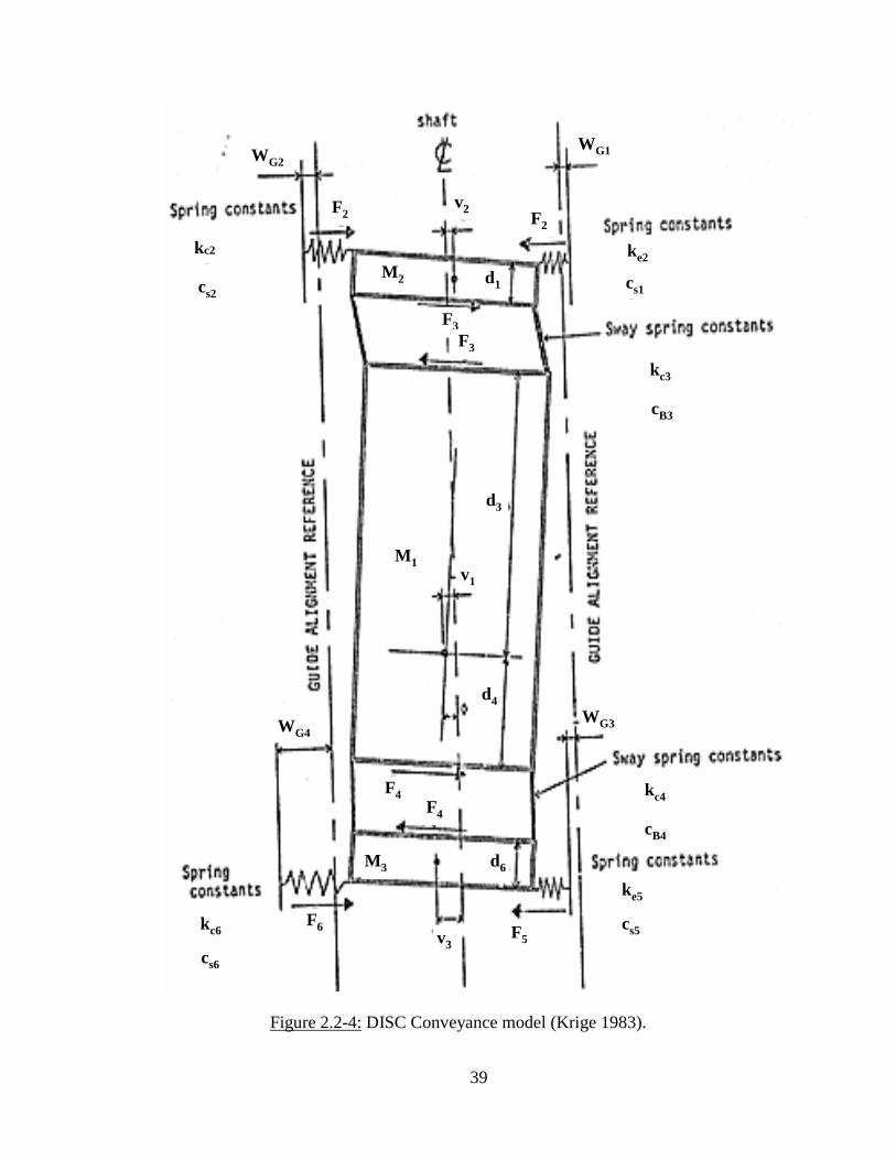
39

kc2

cs2

ke2

cs1

WG1 WG2

kc3

cB3

kc4

cB4

ke5

cs5 kc6

cs6

F2 F2

F3

F3

F4 F4

F5 F6

M2

M1

M3

d3

d1

d4

d6

v1

v2

v3

WG4 WG3

Figure 2.2-4: DISC Conveyance model (Krige 1983).

40

For each degree of freedom, an equation of motion could be presented in its

simplified form, neglecting the damping effect, as follows:

M1 𝑣1 + A5 𝑣1- Kc3 𝑣2- Kc4 𝑣3+ A6𝜑 = 0

M2 𝑣2 - Kc3 𝑣1+ A7 𝑣2 + 0 + A8𝜑 = 0

M3 𝑣3 - Kc4 𝑣1+ 0 + A9 𝑣2 + A9𝜑 = 0

Ir - A1 𝑣1+ A2 𝑣2 + A3 𝑣2+ A4 𝜑 = 0 Equation 2-13

where: A1 = Kc3 𝑑1

2 + Kc3 𝑑3 - Kc4 𝑑4 - Kc4

𝑑6

2

A2 = Ke1 𝑑1

2 + Ke2

𝑑1

2 - Kc3

𝑑1

2 - Kc3𝑑3

A3= Kc4 𝑑4 + Kc4 𝑑6

2 - Ke5

𝑑6

2 - Ke6

𝑑6

2

A4 = Kc3 𝑑1

2 𝑑3 + Kc3 𝑑3

2 + Kc4 𝑑4

2 + Kc4

𝑑6

2 𝑑4

A5 = Kc3 + Kc4

A6 = Kc3 𝑑3 - Kc4 𝑑4

A7 = Ke1 + Ke2 + Kc3

A8 = Kc3 𝑑3

A9 = Kc4 + Ke5 + Ke6

A10 = Kc4 𝑑4

Ke is the effective stiffness of the wheels and guides, Kc is the stiffness of the sway

connections, d is the height of each mass or the distance from the c.g. of the middle mass,

as shown in Figure 2.2-4, M is the mass of each skip part, Ii is the moment of inertia of

the mass of each rigid body, 𝑣𝑖 is the displacement degree of freedom of mass i, and 𝜑 is

the rotational degree of freedom of the total mass.

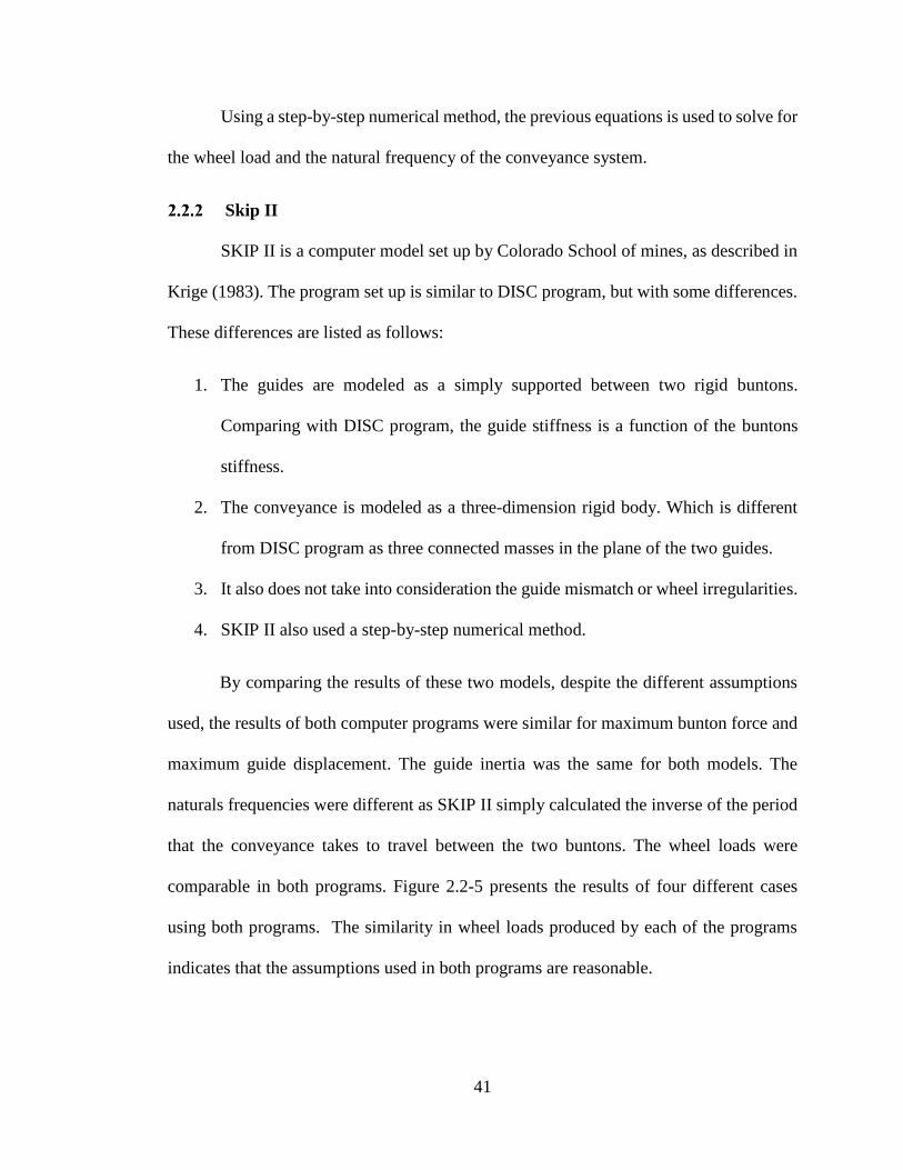
41

Using a step-by-step numerical method, the previous equations is used to solve for

the wheel load and the natural frequency of the conveyance system.

Skip II

SKIP II is a computer model set up by Colorado School of mines, as described in

Krige (1983). The program set up is similar to DISC program, but with some differences.

These differences are listed as follows:

1. The guides are modeled as a simply supported between two rigid buntons.

Comparing with DISC program, the guide stiffness is a function of the buntons

stiffness.

2. The conveyance is modeled as a three-dimension rigid body. Which is different

from DISC program as three connected masses in the plane of the two guides.

3. It also does not take into consideration the guide mismatch or wheel irregularities.

4. SKIP II also used a step-by-step numerical method.

By comparing the results of these two models, despite the different assumptions

used, the results of both computer programs were similar for maximum bunton force and

maximum guide displacement. The guide inertia was the same for both models. The

naturals frequencies were different as SKIP II simply calculated the inverse of the period

that the conveyance takes to travel between the two buntons. The wheel loads were

comparable in both programs. Figure 2.2-5 presents the results of four different cases

using both programs. The similarity in wheel loads produced by each of the programs

indicates that the assumptions used in both programs are reasonable.

42

Figure 2.2-5: Comparing the results from DISC and SKIP II (Krige 1983).

SLAM

As discussed in the inactive-roller configuration earlier in this chapter, SLAM

computer program was created to calculate the extreme slam load created by the slippers

WH

LO

AD

(k

N)

WH

LO

AD

(k

N)

WH

LO

AD

(k

N)

WH

LO

AD

(k

N)

WH

LO

AD

(k

N)

WH

LO

AD

(k

N)

WH

LO

AD

(k

N)

WH

LO

AD

(k

N)

Case 1

Case 2

Case 3

Case 4

TIME (second)

TIME (second)

TIME (second)

TIME (second)

TIME (second)

TIME (second)

TIME (second)

TIME (second)

(a) DISCS (b) SKIP II

00 0 2 4 6 8 0 2 4 6 8

0 1 2 3 4

0 2 4 6 8

0 1 2 3 4

0 2 4 6 8

0 1 2 3 4

0 1 2 3 4

0

3

6

0

3

6

0

3

6

0

3

6

0

3

6

0

3

6

0

3

6

0

3

6

43

Figure 2.2-6: Slam force diagram on different locations of

the skip slipper on the steel guide (COMRO 1990).

located on the side of the skip. Detailed information about the program was found in

COMRO (1990) mineshaft steelwork design guideline. The program integrates the

equation of motion at a small time step to evaluate the forces on the steelwork during

impact. Figure 2.2-6 presents five different slamming events for the same skip-guide

configuration.

Each of the curves presented in the figure is associated with a different initial

contact location on the guide. The first curve the initial contact occurred at 20% of the

distance between the two buntons, the second is at 40% etc. The most critical event

occurred when the skip was closest to the bunton. The last curve shows the impact at the

bunton which is not as severe as just before the bunton event (80%).

44

Table 2.3-1: Shaft Category, Design and Performance Parameters (Comro1990 &

SANS 10208-4).

To build the equation of motion, SLAM used an approximation method while

reducing the skip-guide system to a single degree of freedom (SDOF) system. Some

assumptions were made based on previously completed researched systems as discussed

to this point in the chapter. To create this equivalent SDOF system, multiple parameters

needed to be calculated such as effective mass, effective stiffness and effective applied

force. This phenomenon will be explained in the design procedures of the mineshaft

steelwork provided by the COMRO guideline (1990).

Design procedures

To facilitate the design procedure, shafts were categorized according to the

frequency of mine maintenance. The maintenance includes realignment of guides and

adjusting the rollers. The shafts are categorized as shown in Table 2.3-1.

45

In Table 2.3-1, shafts are divided into four different categories. Each category

demonstrates the maintenance, realignment frequency and their effect on guide

misalignment and slamming data. Comro suggests that designers should consider using a

more conservative category while calculating the slamming load. The example provided

in Appendix A use category C, with a maximum guide misalignment 20mm and gauge

10mm, resulting in the maximum expected slamming load for the mineshaft design.

Shaft steelwork design

After deciding the category of the shaft, the designer should design the shaft

steelwork while taking into consideration that the shaft could:

Minimize the probability of slam events.

Does not fail due to fatigue or under extreme dynamic loads.

Ensure that the skip would be guided at all times.

The following guideline provided by Comro (1990) describes the calculation

procedures to ensure the design of a safe steelwork satisfying the previous criteria.

Steelwork stiffness

To predict the maximum bunton force and deflection, multiple parameters needed

to be determined in the calculations related to every shaft steelwork and skip. Firstly, the

steelwork stiffness, the effective stiffness, is essential for the calculation of the dynamic

response of the system. The steelwork stiffness could be divided into two: stiffness at the

guide midspan (kg) and guide to bunton connection stiffness (kb). Computer calculation is

recommended to analyze the steelwork stiffness.

In the case of flexible skip, where the stiffness of skip is relatively small, the

stiffness of the skip (ks) could be used to estimate a new effective bunton stiffness. The

46

stiffness should be calculated at the slipper plate mount and in the plane of the slamming

load. This effective bunton stiffness could be calculated by putting bunton stiffness kb and

skip stiffness ks in series (Equation 2-14). On the other hand, if the skip stiffness is very

high, the bunton stiffness will be used in the calculations and skip stiffness will not be

considered in the effective stiffness calculation (see the analysis section of this chapter).

𝑘𝑏𝑒 =𝑘𝑏𝑘𝑠

(𝑘𝑏+𝑘𝑠) Equation 2-14

As discussed in the inactive-roller configuration, it is clear in the previous formula

that the guide stiffness is not considered in the effective stiffness. The guide stiffness

would be considered in calculating the impact and the rebound velocities.

Effective skip mass

During slamming events, the skip’s inertia force act on the guide at the slipper

location on the leading corner of the skip. There would be two degrees of freedom

associated with the skip system. The first degree of freedom is the transitional degree of

freedom acting on the center of gravity of the skip. The second degree of freedom is the

rotation about the center of gravity. This behavior is similar to system 4.

The new effective skip mass is calculated as follows:

𝑚𝑒 =𝑚𝑠𝐼

(𝐼+𝑚𝑠ℎ2) Equation 2-15

where: me is effective skip mass during impact, ms is total skip mass, I is the mass

moment of inertia of the skip through the skip c.g. and about an axis normal to the plane

between the guides, and h is the vertical distance between the skip cg and the corner at

47

which me is effective or the distance between skip c.g. and the slipper located at the skip

corner (see Figure 2.3-1).

Analysis

To facilitate the skip behavior analysis, COMRO (1990) provided a list of

parameters that could be defined as follows:

The ratio between the bunton and the midspan guide stiffness (rk) is used to

facilitate the slam load calculation. This ratio is always bigger than 1 as the bunton is

much stiffer than the guide.

rk = 𝑘𝑏

𝑘𝑔 Equation 2-16

In case of flexible skip, the bunton effective stiffness could be used instead of the

bunton stiffness.

Figure 2.3-1 The Geometry of the mine skip and the location of the

effective mass (COMRO 1990)

48

The maximum impact velocity (u) is calculated as shown in the following

equation:

u= 2𝑒𝑣

𝐿 Equation 2-17

Where L is the distance between two buntons, v is the skip hoisting speed, and e is the

maximum guide misalignment depending on the maintenance frequency (see Table 2.3-

1). A ratio of rebound velocity to the impact velocity u could be also represented as ru.

To generalize the impact calculation, multiple non-dimensional factors could be

introduced:

𝑘𝑏 = nondimensional steelwork stiffness at bunton

𝑘𝑏 =

𝑘𝑏𝑒𝐿2

𝑚𝑒𝑣2 Equation 2-18

= nondimensional bunton force

=𝑃𝐿


where: P is the bunton impact force.

𝛿= nondimensional skip displacement

𝛿=𝛿𝑠

𝐿 Equation 2-20

where: 𝛿𝑠 is the skip displacement relative to steelwork in meter.

= nondimensional guide bending moment

49

= 𝑀


where: M is the guide bending moment in N.m.

Knowing the steelwork stiffness ratio (rk) and the non-dimensional stiffness of the

steelwork bunton ( 𝑘𝑏 ), Figures A.2-1 to A.2-4 (see Appendix A) could be used to

determine all relevant steelwork parameters. Note these figures are only for u/v = 0.005.

For different u/v, a correction factor should be applied to P, 𝛿𝑠 and M = 2e/0.005L. The

example, provided in Appendix A, illustrates the procedure for designing the steelwork

of a mine shaft without taking into consideration the roller and fatigue designs.

The slippers should also be designed for fatigue loadings. The designer should

consider the fatigue loads based on the number of impact events. According to the

Commentary on SABS 0208:4 (2001), the slipper plate impact loads occur 10% times of

the hoisting cycles. In an average mineshaft, the impact event could occur 1,000 times per

year.

Dynamic response using Newmark β method

Up to this point of this chapter, an extensive understanding for the dynamic behavior

of the skip/steelwork system was presented. Also, the Comro (1990) guideline was used

to evaluate the impact force in a skip system after approximating the system to a SDOF

system with an effective mass, effective stiffness and an initial impact velocity. In this

portion of the chapter, three different numerical methods will be presented to evaluate the

dynamic behavior of the SDOF system as presented by Biggs (1964). One of these

50

numerical methods will be used to check the analysed example in Appendix A with

Comro guideline.

Building the SDOF model

The single degree of freedom system, as presented in Figure 2.5-1, consists of an

effective mass of the skip, effective stiffness of the bunton and skip, and initial velocity

which will be considered as the impact velocity of the skip. For this system, the applied

force has a very small time interval, thus, the force could be replaced by an impact

velocity. The equation of motion could be presented as follows:

𝑚𝑒 + 𝑘𝑒𝑦 = 𝑓(𝑡) Equation 2-22

where y is the mass displacement and is the mass acceleration.

The damping effect of the system is not considered as it does not affect the initial

impulse of the system vibration. The applied force is considered equal to zero and replaced

by the skip impact velocity (u) which could be calculated using Equation 2-16. The spring

force key is assumed to have a linear spring constant equal to the effective stiffness

calculated using Equation 2-14. The effective mass could be calculated using Equation 2-

15. The equation of motion as presented in Equation 2-21 could be solved using step by

𝑦, 𝑦ሶ , &

𝑘𝑒

𝑚𝑒 𝑓(𝑡)

Figure 2.5-1: Single degree of freedom set up

51

step to determine the variation of displacement and the change in acceleration. Biggs

(1964) presented three different methods to solve the equation of motion:

Constant velocity or lumped-impulse.

Linear acceleration method.

Newmark β method.

The equation of motion could be solved step by step method starting at zero time

when the initial velocity and displacement are known. The time scale is divided into small

intervals which simplify the calculation of displacement from one interval to another.

Constant velocity or lumped-impulse

This analysis considers a constant acceleration between two time steps. Figure 2.5-

2 presents the analysis of the displacement-time variation for a single degree of freedom.

The displacement 𝑦(𝑠) is the mass displacement at time s and 𝑦(𝑠−1) is the

displacement at time s-1 which were previously determined. The acceleration (𝑠) at time

Figure 2.5-2: Numerical Integration using constant velocity method (Biggs 1964)

52

s could calculated using the equation of motion. The displacement 𝑦(𝑠+1) could be

determined using the following equation:

𝑦(𝑠+1) = 𝑦(𝑠)+ 𝑦ሶ𝑎𝑣 ∆t Equation 2-23

where 𝑦ሶ𝑎𝑣 is the average velocity between time stations s and s+1, and ∆t is the time steps

between the stations. 𝑦ሶ𝑎𝑣 could be determined by:

𝑦ሶ𝑎𝑣 = 𝑦(𝑠)−𝑦(𝑠−1)

∆t + (𝑠)∆t Equation 2-24

The average velocity could be presented as the average between the velocity at

time s-1 and s added to the increase in the velocity exercised by the acceleration of the

system in the time interval while assuming (𝑠) is the average acceleration over the

interval. Using these approximation, the curves into straight lines facilitate the calculation

of the displacement on the next time station. Substituting Equation 2-24 in 2-23:

𝑦(𝑠+1) =2𝑦(𝑠) − 𝑦(𝑠−1) + (𝑠)(∆t) 2 Equation 2-25

Although, Equation 2-25 is approximated, but it could present an accurate solution

by minimizing the time step (∆t ⟶ 0). The solution in this situation approaches the exact

solution, however, the number of computations will increase. In most cases, to find an

accurate solution with less computation, the time step could be assumed equal to the one-

tenth of the natural period of the system.

In some cases, 𝑦(𝑠−1) has no value as the analysis could start at t = 0 where

different approach should take place to progress with the analysis. Two different

procedures could be used. First, the acceleration could be assumed to be linear on the

first time interval. The displacement could be calculated:

53

𝑦(1) = 1

6 (2(0) + (1))(∆t) 2 Equation 2-26

Second, the acceleration could be assumed constant:

𝑦(1) = 1

2 (0)(∆t) 2 Equation 2-27

However, Equation 2-27 should be used if the dynamic problem does not have

an external force. Therefore, the acceleration will be equal to zero. In case of problem

instability or convergence, more accurate methods could be used. The following

numerical methods satisfy greater precision for the same time step used in the constant

velocity method.

Linear-acceleration method

This method is a small adjustment for the previous constant-velocity method by

assuming a linear acceleration function (see Figure 2.5-3). If the acceleration is assumed

to be linear between two time steps, the acceleration could be presented by:

= (𝑠) + (𝑠+1)−(𝑠)

∆t (𝑡 − 𝑡(𝑠)) Equation 2-28

The velocity at the same time interval:

𝑦ሶ = 𝑦ሶ (𝑠) + (𝑠)(𝑡 − 𝑡(𝑠)) + (𝑠+1)−(𝑠)

2∆t (𝑡 − 𝑡(𝑠)) Equation 2-29

The velocity at s+1:

𝑦ሶ (𝑠+1) = 𝑦ሶ (𝑠) +∆t

2 ((𝑠+1) + (𝑠)) Equation 2-30

The displacement at s+1:

54

𝑦(𝑠+1) =𝑦(𝑠) + 𝑦ሶ (𝑠)∆t +(∆t)2

2(2(𝑠) + (𝑠+1)) Equation 2-31

The velocity at s as presented in Equation 2-30:

𝑦ሶ (𝑠) = 𝑦ሶ (𝑠−1) +∆t

2 ((𝑠) + (𝑠−1)) Equation 2-32

Equation 2-31 and 2-32 are the basis for the linear acceleration numerical method.

As presented in Equation 2-31, in order to obtain 𝑦(𝑠+1), (𝑠+1) should be obtained

first. Nonetheless, (𝑠+1) is also depending on 𝑦(𝑠+1). To solve this problem, the equation

of motion should be used:

(𝑠+1) =𝐹(𝑡(𝑠+1))

𝑀−

𝑘

𝑀 𝑦(𝑠+1) Equation 2-33

By combining Equation 2-33 and 2-31:

Figure 2.5-3 Linear-acceleration approximation (Biggs 1964)

55

𝑦(𝑠+1) = 𝑦(𝑠)+ 𝑦ሶ (𝑠)∆t +

(∆t)2

3 (𝑠) +

(∆t)2

6 𝐹(𝑡(𝑠+1))

𝑀

1+(∆t)2

6

𝑘

𝑀

Equation 2-34

The newly developed equation along with Equation 2-32 presents a direct solution for

𝑦(𝑠+1). This method solves the dynamic problem more accurately.

Newmark β method

A multipurpose method developed by Newmark that could be adjusted to satisfy

different problems. The equations created by Newmark:

𝑦ሶ (𝑠+1) = 𝑦ሶ (𝑠) +∆t

2 ((𝑠) + (𝑠+1)) Equation 2-35

And 𝑦(𝑠+1) =𝑦(𝑠) + 𝑦ሶ (𝑠)∆t + (1

2− β) (𝑠)(∆t)2 + β(𝑠+1)(∆t)2 Equation 2-36

β could be selected depending the assumed acceleration in the specific time step.

The value selected affects the convergence in every time step, the stability of the system,

and the amount of accuracy. β value could be affected by the time step value. After

investigating the method, the best results could be obtained if β is between 1

6 and

1

4 and

∆t is between 1

6 and

1

5 of the shortest natural period.

Numerical integration by spreadsheet

A spreadsheet was developed using the information provided by Chopra (2006) to

reformulate Newmark’s equations. Chopra modified Equation 2-35 to prevent iteration

using incremental quantities as follows:

∆𝑦𝑠 ≡ 𝑦𝑠+1 − 𝑦𝑠 ∆𝑦ሶ 𝑠 ≡ 𝑦ሶ 𝑠+1 − 𝑦ሶ 𝑠 ∆𝑠 ≡ 𝑠+1 − 𝑠

56

∆𝑓𝑠 ≡ 𝑓𝑠+1 − 𝑓𝑠 Equation 2-37

These incremental forms are used for the analysis of non-linear system. Substituting the

incremental forms in Equation 2-35 & 2-36:

∆𝑦ሶ (𝑠) = (∆t )(𝑠) + (𝛾∆t )(𝑠)

And ∆𝑦(𝑠) = 𝑦ሶ (𝑠)∆t +(∆t)2

2 (𝑠) + β ∆(𝑠)(∆t)2 Equation 2-38

The acceleration incremental form is presented as:

∆(𝑠) =1

β(∆t)2 ∆𝑦(𝑠) − 1

β ∆t 𝑦ሶ (𝑠) −

1

2β(𝑠) Equation 2-39

Substituting Equation 2-39 in Equation 2-38:

∆𝑦ሶ (𝑠) =𝛾

β ∆t ∆𝑦(𝑠) −

𝛾

β 𝑦ሶ (𝑠) + ∆t(1 −

𝛾

2β )(𝑠) Equation 2-40

Equation 2-39 and 2-40 could be substituted in an incremental equation of motion:

m∆(𝑠) + 𝑘 ∆𝑦(𝑠) = ∆𝑓(𝑠) Equation 2-41

𝑘 ∆𝑦(𝑠) = ∆𝑓(𝑠) Equation 2-42

where

𝑘 = 𝑘 + 1

β(∆t)2 m Equation 2-43

And

57

∆𝑓(𝑠) = ∆𝑓(𝑠) +1

β ∆t𝑚 𝑦ሶ (𝑠) +

1

2β 𝑚(𝑠) Equation 2-44

With 𝑘 and ∆𝑓(𝑠) are calculated knowing the mass and the stiffness of the system and the

initial velocity and acceleration at the beginning of the first time step. The incremental

displacement is calculated:

∆𝑦(𝑠) = ∆(𝑠)

𝑘 Equation 2-45

After calculating ∆𝑦(𝑠) using Equation 2-45, 𝑦ሶ (𝑠) 𝑎𝑛𝑑 (𝑠) are be computed using

Equation 2-39 and Equation 2-40. The acceleration of the next time step is calculated as

follows:

(𝑠+1) = 𝑓

(𝑠+1)−𝑘𝑦(𝑠+1)

𝑚 Equation 2-46

Two special cases for Newmark’s method are presented as follows:

The average acceleration method by substituting (𝛾 =1

2 , 𝛽 =

1

4).

The linear acceleration method by substituting (𝛾 =1

2 , 𝛽 =

1

6).

The following steps were used to build the stepping spreadsheet using Newmark’s

method (Chopra 2011):

a) Initial calculations:

i. Calculating the initial acceleration using Equation 2-46.

ii. Select time step suitable for the system.

iii. Calculating 𝑘 using Equation 2-43.

58

iv. Calculating: 𝑎 = 1

β ∆t𝑚 and 𝑏 =

1

2β 𝑚

b) Calculations for each time step (s):

i. ∆𝑓(𝑠) = ∆𝑓(𝑠) + 𝑎 𝑦ሶ (𝑠) +𝑏 (𝑠)

ii. ∆𝑦(𝑠) = ∆(𝑠)

𝑘

iii. ∆𝑦ሶ (𝑠) =𝛾

β ∆t ∆𝑦(𝑠) −

𝛾

β 𝑦ሶ (𝑠) + ∆t(1 −

𝛾

2β )(𝑠)

iv. ∆(𝑠) =1

β(∆t)2 ∆𝑦(𝑠) − 1

β ∆t 𝑦ሶ (𝑠) −

1

2β(𝑠)

v. 𝑦(𝑠+1) = 𝑦(𝑠) + ∆𝑦(𝑠), 𝑦ሶ (𝑠+1) = 𝑦ሶ (𝑠) + ∆𝑦ሶ (𝑠), (𝑠+1) = (𝑠) + ∆(𝑠)

c) Step b will be repeated for every time step.

The spreadsheet was built using the following assumptions:

The effective mass calculated in Appendix A was used as the mass of the

system.

The effective bunton stiffness calculated in Appendix A was used as the

system’s stiffness. The stiffness was considered as a constant stiffness.

The initial velocity of the system was assumed equal to the impact velocity

calculated in Appendix A.

The initial acceleration, initial displacement, and the external force were

assumed equal to zero as, at time zero, the skip and the bunton would act

as a single system at the initial contact.

To transfer Newmark’s method to linear acceleration method, the values

of 𝛾 𝑎𝑛𝑑 𝛽 were used 1

2 𝑎𝑛𝑑

1

6 respectively.

59

A sample of the spreadsheet, used to calculate the example in Appendix A, is

presented in Figure 2.5-4.

Figure 2.5-4 A Sample Calculation for the SDOF Spreadsheet

The spreadsheet presents the step numerical analysis for a single degree of

freedom system. At time zero, as shown in Figure 2.5-4, the initial displacement and

acceleration was assumed equal zero. The initial velocity was considered equal to the

impact velocity calculated in Appendix A (0.05m/s). The maximum bunton force (F max)

calculated as the maximum acceleration that the system reach (y”) multiplied by the

effective mass (me) was found equal 20,092 N. A small difference between the calculated

bunton force in Appendix A (20,756 N) and the force calculated using the spreadsheet

(20,092 N) as the result calculated in Appendix A was obtained using a graph presented

by the Comro guideline. Figure 2.5-5 presents a graph of the bunton force harmonic

behavior calculated by the spreadsheet. The maximum deflection (y max) calculated

using the spreadsheet is equal to 3 mm. On the other hand, the guide maximum guide

60

deflection calculated in section 3.5 was equal to 5.6 mm. The reason behind these different

values of deflection is: the maximum deflection in the spreadsheet was calculated at the

bunton location but the guide maximum deflection was calculated using the SLAM

program using the assumption in section 2.1.2 Inactive-rollers configuration and

presented in Figure 2.1-13. The maximum guide deflection does not occur at the bunton

location. Figure 2.5-6 presents a graph of the deflection harmonic behavior calculated by

the spreadsheet.

Figure 2.5-5 The bunton force harmonic response as calculated by the spreadsheet.

-25000

-20000

-15000

-10000

-5000

0

5000

10000

15000

20000

25000

0.00 0.05 0.10 0.15 0.20 0.25 0.30 0.35 0.40

Forc

e (N

)

Time (s)

Impact Force

61

Figure 2.5-6 The deflection harmonic response as calculated by the spreadsheet.

The spreadsheet was built to compare the data calculated using the Comro guideline

and estimate the dynamic behavior of the dynamic test explained in Chapter three. The

damping behavior of the system is not considered as damping will not affect the initial

impact farce magnitude.

Conclusion

In this Chapter, the dynamic behavior of the skip/steelwork system was discussed

including the factors affecting this behavior. These factors could be summarized as

follows:

The misalignment of the shaft guide.

The bunton, skip, and guide stiffness.

The mass of the skip and the hoisting velocity.

The distance between two consecutive buntons.

-0.004

-0.003

-0.002

-0.001

0.000

0.001

0.002

0.003

0.004

0.00 0.05 0.10 0.15 0.20 0.25 0.30 0.35 0.40

Dis

pla

cem

ent

(y)

(m)

Time (s)

Displacement

62

In extreme cases, the bunton and skip stiffness are relatively high. This higher skip

stiffness could be found in the balancing weight behavior (B1) presented in Figure A.1b-

1. Where the balancing weight has higher stiffness than the skip (A1&A2) or man cage

(C1). Also, the bunton stiffness is much higher as it is a fixed concrete bunton, less flexible

than the cantilever bunton used in Skips A1&A2. The hoisting speed could be higher

reaching 15 m/s, the distance between the buntons and the guide misalignment could, also,

increase the impact velocity of the skip which would increase the bunton force. The mass

of the skip has a great effect on the dynamic behavior. The skip mass could reach 130

tons.

This research was conducted to reduce the bunton force in extreme cases. One of

the ways to conduct this reduction is by reducing the skip stiffness at the slipper location

which will reduce the bunton effective stiffness and the bunton force. The skip stiffness

could be reduced by adding a flexible slipper on the sides of the skip. This flexible slipper

could reduce the effective bunton stiffness and the bunton impact force. The following

chapters will discuss the new design of this flexible slipper including the dynamic test of

the CDP material.

63

3 Chapter 3 Experimental procedure

The experimental program consisted of two testing regimes: Static compressive

test and Impact test. This chapter provides details on the testing method and the equipment

used to conduct both tests including the data acquisition systems.

Static compressive test

This test is designed to determine the compression stress-strain characteristics of

rubber bearing pads under static compression or low strain rate loading. This research

focuses on Cotton Duck Rubber Pad (CDP) as discussed in previous chapters. Samples

used in this test was provided by a single manufacturer not taking into consideration other

manufacturers.

Equipment description

This test measures the compressive stiffness of the CDP. Deflection is measured

as the reduction of CDP thickness. The force is measured while applying a constant

deflection rate for the CDP. The following equipment was used to perform the test:

Universal compression testing machine: Instron (see Figure 3.1-1):

The machine consists of a moving head and non-moving bottom. The moving head

is used to apply the load on the CDP specimen while the non-moving bottom holds the

specimen in place. The moving head contains a load cell with a capacity of 250 kN which

was calibrated prior to the tests. The load cell was used to measure the load applied to the

CDP specimen. The movement rate of the head was determined depending on the

thickness of the CDP and the strain rate needed to test the effect of different strain rates

on different rubber pad sizes. The test machine usually moves with the speed needed to

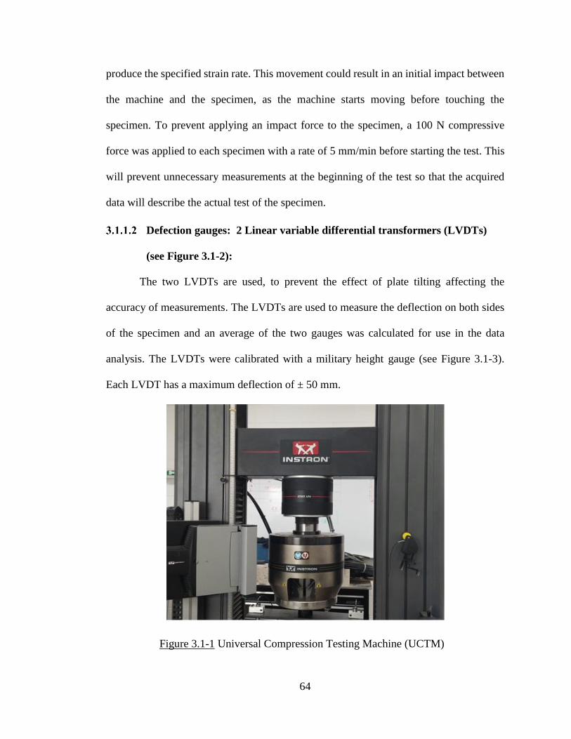
64

Figure 3.1-1 Universal Compression Testing Machine (UCTM)

produce the specified strain rate. This movement could result in an initial impact between

the machine and the specimen, as the machine starts moving before touching the

specimen. To prevent applying an impact force to the specimen, a 100 N compressive

force was applied to each specimen with a rate of 5 mm/min before starting the test. This

will prevent unnecessary measurements at the beginning of the test so that the acquired

data will describe the actual test of the specimen.

Defection gauges: 2 Linear variable differential transformers (LVDTs)

(see Figure 3.1-2):

The two LVDTs are used, to prevent the effect of plate tilting affecting the

accuracy of measurements. The LVDTs are used to measure the deflection on both sides

of the specimen and an average of the two gauges was calculated for use in the data

analysis. The LVDTs were calibrated with a military height gauge (see Figure 3.1-3).

Each LVDT has a maximum deflection of ± 50 mm.

65

Specimen

LVDTs

military height gauge LVDT

Figure 3.1-3 LVDTs calibration using a military height gauge

Figure 3.1-2 LVDTs and Experimental set up

66

A high-speed camera (PFV ver 2.0) (see Figure 3.1-4)

This camera was used in the static test to check the displacement and compare the

Digital Image Correlation (DIC) calculated deflection to the average deflection from the

LVDTs data. This comparison was then used to check the accuracy of the camera to be

used later for measuring the specimen deflection in the impact tests. After multiple trials,

the most accurate displacement data (for this camera) was found using the following

specifications:

Minimum 1 m distance between the object and the camera for good focus and

plane picture.

Maximum frame rate: 5000 frames per seconds.

Minimum resolution of 128×80 pixels. This resolution could vary depending on

the frame rate.

Figure 3.1-4 High-speed camera and light source.

High-Speed

Camera

Light

source

67

Figure 3.1-5 Three specimen sizes: 12.7, 25.4, and 50.8 mm

A source of light

The source of light provided a higher lux for the specimen to acquire video and

pictures for DIC more effectively (see Figure 3.1-4).

Data acquisition

The Instron machine was connected to a computer program recording the data

acquired by the load cell and both LVDTs. The computer software processed the data and

sorted it in a table form for further analysis. The high-speed camera was connected to

another computer to record the frames needed for analysis using digital image correlation

(DIC) with a Matlab program. The use of DIC will be discussed extensively in the impact

test portion of this chapter.

Samples preparation

In the static compression test, the half inch thick specimens were cut into square

40x40 mm2 specimens using a band saw. The 12.7 mm thick specimens were bonded with

epoxy resin (ASTM D-4236) to form different specimen thicknesses: 12.7, 25.4, and 50.8

mm (see Figure 3.1-5). These three sizes were selected to evaluate the shape factor’s effect

on the strength of the CDP, as discussed in Chapter 1.

68

The following table presents the number of specimens used for every loading rate.

These loading rates are used to examine the effect of different strain rate on the behavior

of the CDP. Twenty-eight specimens were used to examine static compression properties

of the material. The numeric system and the measured sizes of the specimens will be

discussed in Chapter 4.

Table 3.1.3-1: Number of specimens used in every loading rate

For every loading rate and specimen thickness the expected strain rate could be

calculated using Equation 3-1 and presented in Table 3.1.3-2:

Expected Strain Rate = loading rate × 60/specimen thickness Equation 3-1

Table 3.1.3-2 Loading rate and expected strain rate for each CDP thickness

Specimen Thickness

(mm)

Loading Rate (mm/min) Expected Strain Rate (s-1)

12.7 12 15.75×10-3

80 105.00×10-3

200 262.50×10-3

400 524.90×10-3

25.4 200 131.20×10-3

400 262.50×10-3

50.8 400 131.20×10-3

Pad

Nominal size

Loading Rate

12 mm/min 80 mm/min 200 mm/min 400 mm/min

40×40×12.8 4 4 4 4

40×40×25.4 4 4

40×40×50.8 4

69

These various specimen’s thicknesses and strain rates will provide a clearer

understanding of the CDP behavior and properties, providing that will be used as a basis

to be compared to the dynamic properties of the CDP.

Summary of the test methodology

The test procedure used is described as follows:

The specimens were cut into the specified dimensions using a band saw as

previously described in Section 3.1.3.

The specimens were centered between the two LVDTs to maintain an accurate

deflection recording. The specimens were centered inside the UCTM to maintain

a well distributed load (see Figure 3.1-2).

Using the computer program associated with the test machine, the loading rate,

maximum load, and maximum deflection were specified to maintain a safe and

effective test procedures.

Before starting a test, the LVDTs and load cell were zeroed to acquire the data

starting from zero points.

The data from the load cell and the two LVDTs were recorded in tabular form

during the test and saved for further analysis.

The recorded data was used to construct stress-strain curves for each specimen

and loading rate.

Impact test

This test was designed to determine the compression force-deflection

characteristics of rubber bearing pads under impact or high strain rate loading. This

70

research was conducted on the same Cotton Duck Rubber Pad (CDP) as discussed in

previous chapters.

Summary of test method and equipment

This test measured the compressive stiffness of the rubber under impact.

Deflection is measured as the reduction of rubber thickness.

Modified Charpy impact load test

Preparing the Charpy machine:

The Charpy impactor was originally used to test the material ductility under

impact load as specified in the ASTM Standard Test Methods for Notched Bar Impact

Testing of Metallic Materials (E23). In this test, a swinging U-shaped hammer strikes the

sample in two locations causing the bending of the sample until fracture. The gauge

records the amount of energy absorbed by the sample to measure its ductility. By adding

a thick plate to the U-shaped hammer and modifying the part holding the sample (support),

the Charpy machine was transformed to an impact machine.

Modifying the hammer:

The most important parameter for plate design is the plate’s stiffness. The stiffer

the plate means less plate deformation and the impact event would only measure the

properties of the rubber sample. The stiffness was calculated: in the case of using a 1”

(25.4mm) thick plate is equal to 2.375x109N/m and for a 2” (50.8mm) thick plate is equal

to 1.900x1010N/m. Both steel plate thicknesses could be used to transform the U-shaped

pendulum hammer to a surface impact tool without affecting the impact data. For this test,

the 1” (25.4mm) plate was used. The hammer and plate arrangement used for the tests is

shown in Figure 3.2-1.

71

The swinging hammer is used to apply the impact load on the rubber specimen.

However, to keep the rubber specimen from moving, a non-moving support was added to

the test mechanism.

Non-moving support design:

A thick steel plate was mounted to a steel frame, bolted to the strong floor, to act

as non-moving support for the impact test. The support design requirements were as

follows:

a) The support was mounted to the strong floor so that the readings would not

be affected by the frame vibrations.

b) The support was assumed to have a high stiffness, so the data measured during

the impact test would only measure the CDP properties.

c) The load was applied perpendicular the specimen.

d) The support was adjustable to accommodate for the change in specimen

thicknesses.

To satisfy the previous requirements, the support components were

designed as shown in Figure 3.2 -2 and described below:

Steel Plate

Figure 3.2-1 The hammer and plate arrangement for impact measurement.

72

a) To maintain a perpendicular load, without inclination, spherical washers were

used to remove any bolt inclination errors (Figure 3.2-2a).

b) One 1 1/8” diameter bolt used to mount the steel plate to the steel frame fixed

to the concrete ground (Figure 3.2-2b). The bolt was used to hold the load cell

in place.

c) Two steel plates to increase the total stiffness of the support and prevent direct

impact on the bolt, providing a smooth surface to mount the specimen. The

mating surfaces of the two plates were surface ground to ensure a good

transfer of load between the plates and reduce friction losses (Figure 3.2-2d).

d) Eight small bolts were used to hold the two plates together (Figure 3.2-2e and

f).

73

(a)

(f)

(c)

(b)

(e)

Figure 3.2-2 Support design: (a) Spherical washers. (b) the washer, bolt, and first

steel plate. (c) The hole in the steel plate so the bolt could be easily mounted on

the steel frame. (d) Two steel plates surface ground to reduce friction between the

plates. (e) Eight bolts to connect the two plates together. (f) Final look for the

support and the space needed for the load cell and adjusting steel washers.

(d)

74

The modified Charpy machine, including the modified hammer and the support,

is shown in Figure 3.2-3. The body of the Charpy machine (the green frame) was also

mounted to the steel frame, supporting the non-moving portion of the test machine, to

prevent the movement of the machine.

The Charpy machine provides two release positions for the pendulum hammer.

The original impact energy for both positions, as provided by the impact gauge, were

169.4 joules and 406.7 joules. These values are irrelevant in the new configuration as

there is a change in the hammer mass by adding the steel plate and also a change in the

Connection

between the

fixed steel

frame and the

Charpy frame.

Figure 3.2-3 Modified Charpy, Impact Testing Machine.

75

support configuration (see Figure 3.2-4). The two release positions were used to provide

different impact forces to measure the rubber properties under higher strain rates.

An accelerometer was mounted on the hammer’s plate to measure the acceleration

of the hammer to calculate the applied impact force. To verify the data from the

accelerometer, a load cell was located at the support. The following section will discuss

these sensors in more details.

Two sensors: an accelerometer and a full bridge load cell:

A one dimension shock accelerometer designed to measure up to 5000 g

(equivalent to 49050 m/s2) (see Figure 3.2-5), used for testing was calibrated by the

manufactuer with a calibration factor of 0.263 mV/V/g. The accelerometer was mounted

Figure 3.2-4 Two pendulum hammer positions for the Charpy machine.

76

to the back of the steel plate fixed on the Charpy hammer using a tapped hole to accept

the threaded stud at the base of the accerometer. To calculate the impact force on the

specimen, measured mass of the hammer and plate was multiplied by the acceleration data

acquired during the impact event. The hammer total mass was equal to 35.7 Kg.

A customized full bridge load cell was used to check the data acquired by the

accelerometer. The load cell was fabricated with four strain gauges mounted on the load

cell to form a full bridge using a Wheatstone bridge configuration (see Figure 3.2-6).

Figure 3.2-5 One Dimension Shock Accelerometer.

Figure 3.2-6 Wheatstone Full Bridge compression configuration (NI 2016).

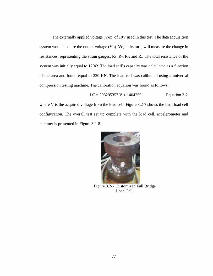
77

Figure 3.2-7 Customized Full Bridge

Load Cell.

The externally applied voltage (Vex) of 10V used in this test. The data acquisition

system would acquire the output voltage (Vo). Vo, in its turn, will measure the change in

resistances, representing the strain gauges: R1, R2, R3, and R4. The total resistance of the

system was initially equal to 120Ω. The load cell’s capacity was calculated as a function

of the area and found equal to 320 KN. The load cell was calibrated using a universal

compression testing machine. The calibration equation was found as follows:

LC = 208295357 V + 1404259 Equation 3-2

where V is the acquired voltage from the load cell. Figure 3.2-7 shows the final load cell

configuration. The overall test set up complete with the load cell, accelerometer and

hammer is presented in Figure 3.2-8.

78

Two steel washers with 25mm and 37.5 mm thicknesses

To accommodate the change in specimen sizes and to maintain the impact load

perpendicular to the surface of the specimen, two steel washers one 25mm thick and the

other 37.5 mm thick were fabricated (see Figure 3.2-9). These washers were located at

the load cell’s location to adjust the support to maintain horizontal impact of the hammer

on the specimen without having to move the Charpy green frame. The 25mm washer was

used to adjust the support location of the 25.4 mm samples. The 37.5mm washer was used

to adjust the location of the 12.7 mm samples. The washers have an extended edge to hold

the load cell in place so that the load cell transfers the load completely from the plate

through the washer to the support.

Accelerometer

mounted to the

steel plate from

inside the

hammer

Load Cell

Figure 3.2-8 Overall set up for accelerometer and load cell in modified Charpy

testing machine.

79

The high-speed camera (see Figure 3.1.3-4)

As previously described in the static compression test, the high-speed camera

recorded images of different stages of the impact event. These images would be used in

the DIC analysis.

A Source of light

The source of light provided a higher lux for the specimen to acquire video and

pictures for DIC more effectively (see Figure 3.1-4).

Data acquisition

Two data acquisition systems were used in this test:

NIcDAQ-9172 series C (see Figure 3.2-10) was used as the data acquisition

system for these tests. A NI9205 strain gauge card was used to monitor load through the

load cell. A NI9237 card was used to monitor acceleration of the hammer. The data was

recorded at sample rate of 50,000 samples/second for each measurement. More

information is provided in Appendix B.

Figure 3.2-9: Two washers with thicknesses 25 mm and 37.5 mm.

80

A high-speed camera was used to monitor the side view of the specimen during

impact response. The camera recorded 5000 frames/second. These recorded images were

used to measure displacement response using digital image correlation. The digital image

correlation was used to measure the CDP deflection. Digital image correlation is a white

light technique based on comparing images before and after deformation of the sample

by comparing the degree of white colour in each pixel of the picture. To facilitate the

pictures comparison, a common method was used to change the colour of the specimen

surface to form a black and white random pattern. This method is called speckling. The

speckling procedures is discussed in the specimen preparation portion of this

experimental program. A monochromatic camera could be used to capture the stages of

the test forming an array of pixels for each picture. Detecting the movement of pixels was

facilitated by defining a greyscale level for each pixel. An open source matlab program

(NCORR V2) was used to calculate the movement of pixels in consecutive images to

NI 9237 NI 9205

Channel

Figure 3.2-10 NI cDAQ-9172 model and both NI9205 and NI9237 Cards.

81

calculate the deflection of the samples over time. For higher strain rates, the DIC’s high

accuracy could be achieved by using a higher frame rate.

Samples preparation

Samples used for impact tests were prepared using the same method as for the

static test. The result was three different specimen thicknesses: 12.7, 25.4, and 50.8 mm

(see Figure 3.1-4). In the impact tests, speckling all samples was essential, creating a

random pattern to facilitate the DIC analysis. This pattern could be produced by 2 different

methods: 1- spray 2- airbrush. The sample was colored with a white color. Using a black

spray or a brush containing black color, black dots was spread over the white surface of

the specimen. The result should appear as presented in Figure 3.2-11.

This pattern was developed by coloring the background with white and then use a

black spray to form a pattern of a mixed black and white speckles. The pattern of the CDP

rubber is not random, as it is formed with overlaying lines (see Figure 3.2-12). This lines

pattern could affect the digital image correlation, affecting in tern the displacement

measurement.

Figure 3.2-11 Random speckled surface.

82

The following table presents the number of specimens used for both Charpy

position. The total number of specimens used for the impact test was 24 specimens. The

numeric system and the measured sizes of the specimens is discussed in Chapter 4.

These various specimen’s thicknesses and Charpy positions will give an extensive

understanding of the CDP behavior and properties under impact (dynamic) loading. The

following chapter will discuss the experimental results based on the methods used in this

chapter.

Table 3.2.3-1 Number of specimens used for each Charpy position.

Summary of the test methodology

The test procedure is described by the following steps:

The specimen was cut into the specified dimensions.

The specimen was speckled by coloring the surface with white color and using a

black spray to form a random pattern of black and grey dots.

The specimen was mounted to the support plate perpendicular to the hammer

Pad Nominal size Charpy position 1 Charpy position 2

40×40×12.7 4 4

40×40×25.4 4 4

40×40×50.8 4 4

Figure 3.2-12 CDP pattern before speckling.

83

The high-speed camera and the light was adjusted to acquire the needed pictures

for analysis.

The accelerometer and the load cell were connected to the NI cDAQ-9172 to

acquire to data needed.

The hammer was latched to either of the two positions.

Both Data acquisition system were triggered at the same time.

The programs were designed to acquire 10 seconds’ worth of data to reduce the

time required for extracting the test data.

The final acquired data was used to build a stress-strain curve for the loading and

unloading for each specimen and Charpy location.

84

4 Chapter 4 Experimental Results

This chapter discusses the experimental results for the testing methods presented

in chapter 3. Both methods were used to study the behavior of the Cotton Duck Pad (CDP)

material under static compression loading and impact loading. The CDP properties,

developed in this chapter, were used to design a new flexible skip slipper plate to reduce

the bunton slam load force as discussed in Chapter 2. This Chapter is divided into two

parts: Part one presents the results of 28 CDP samples static compression tests with

different loading rates; Part 2 presents the results of 24 CDP samples impact tests with

two different Charpy positions.

Static compression test results

The 2B static compression tests were conducted using a universal compression

testing machine following the static test procedures presented in Chapter 3. The testing

machine recorded the applied force measured using the load cell and the displacement

with two LVDTs. The data from both LVDTs are used to calculate the average

displacement. Before testing, the dimensions of each specimen were measured and

recorded (see Table 4.1-1). Each dimension was calculated based on the average of three

measurements. The average displacement, applied force, and the measured dimensions of

the sample were used to develop stress-strain curves for each sample. Every four samples

were used to create a lab report. Each lab report was used to describe the behavior of

CDPs samples with different strain rate and thickness combination. The samples names,

presented in Table 4.1-1, are described as: the letters show different samples for the same

85

test set and the number used to define different test set thicknesses and loading rates

combination.

Table 4.1-1: Dimensions, test type, and loading rate for each sample for tests 1 to 7.

Detailed results for each test set are presented in lab reports provided in Appendix

C. Each report present:

Sample

name

Average

measured

thickness

(mm)

Average

measured

length

(mm)

Average

measured

width

(mm)

Area

(mm2)

Test type Loading

rate

(mm/min)

A-1 11.80 42.60 40.70 1733.82 Compression 12

B-1 12.24 40.60 39.85 1617.91 Compression 12

C-1 12.75 38.51 39.50 1521.15 Compression 12

D-1 12.52 40.70 38.80 1579.16 Compression 12

A-2 12.52 40.10 38.90 1559.89 Compression 80

B-2 12.73 40.20 39.80 1599.96 Compression 80

C-2 12.80 40.90 39.90 1631.91 Compression 80

D-2 12.54 40.70 39.90 1623.93 Compression 80

A-3 12.35 39.80 40.60 1615.88 Compression 200

B-3 12.40 40.50 40.10 1624.05 Compression 200

C-3 12.60 39.70 40.05 1589.99 Compression 200

D-3 12.80 41.80 40.40 1688.72 Compression 200

A-4 12.50 40.02 40.50 1620.81 Compression 400

B-4 12.48 40.85 40.40 1650.34 Compression 400

C-4 12.53 40.45 40.75 1648.34 Compression 400

D-4 12.55 38.60 40.70 1571.02 Compression 400

A-5 25.10 40.50 40.20 1628.10 Compression 160

B-5 25.50 40.70 40.10 1632.07 Compression 160

C-5 25.20 40.50 41.00 1660.50 Compression 160

D-5 25.30 41.50 40.50 1680.75 Compression 160

A-6 25.20 40.60 39.95 1621.97 Compression 400

B-6 24.85 40.00 40.20 1608.00 Compression 400

C-6 25.50 39.75 40.70 1617.83 Compression 400

D-6 25.10 40.35 40.20 1622.07 Compression 400

A-7 50.40 40.10 40.20 1612.02 Compression 400

B-7 50.35 40.50 40.20 1628.10 Compression 400

C-7 50.90 40.50 40.80 1652.40 Compression 400

D-7 50.30 40.30 40.10 1616.03 Compression 400

86

Test description including the experimental set up as described in Chapter 3,

loading rate and specimen dimensions.

Test results for one sample including strain vs time for both LVDTs data (see

Figure 4.1-1) and stress- strain curve for both LVDTs data (see Figure 4.1-2).

Figure 3.2.4-1 Strain rates from 2 LVDT and their average for sample A-1

Figure 3.2.4-2: Strain rates from 2 LVDT and their average for sample A-1

Stress-strain curve for all four samples and their average (see Figure 4.1-3).

0.00

0.05

0.10

0.15

0.20

0.25

0.30

0.35

0.40

0 5 10 15 20 25 30

Stra

in (

mm

/mm

)

Time (sec)

Strain-1-A-1

Strain-2-A-1

Average

0

20

40

60

80

100

120

0 0.05 0.1 0.15 0.2 0.25 0.3 0.35

Stre

ss (

MP

a)

Strain (mm/mm)

LVDT1-A-1

LVDT2-A-1

Average

87

Figure 3.2.4-3: The Stress-strain curves of the four samples tested under 12mm/min

loading rate and their average (S-1-Average)

Observations and discussions for each test.

4.1.1 Discussion & summary

The lab reports (see Appendix C) present the data for each test without comparing

the tests results. In the following sections the effect of eccentric loading, comparison of

the results, and DIC results for static test are presented.

4.1.1.1 Effect of eccentric loading

Due to eccentricity of loading for some samples, the difference between the

displacement acquired by the two LVDTs was relatively large. The displacement at each

edge of the specimen was calculated. 2% of the total displacement difference was allowed

0

20

40

60

80

100

120

0.00 0.05 0.10 0.15 0.20 0.25 0.30 0.35 0.40

Stre

ss (

MP

a)

Strain (mm/mm)

S-1-Average

S-A-1

S-B-1

S-C-1

S-D-1

88

between the two edges of the CDP specimen, to minimize the rotation effect on CDP

(Roeder 2000). If the difference exceeded 2% of the total displacement, the test was

canceled and the specimen was replaced with a new specimen.

4.1.1.2 Samples failure

As previously discussed, the test program was designed to test the properties of

the CDP material without failure. But, due to change in thickness and loading rates, some

samples reached failure. Figure 4.1.1-1 presents examples of failures occurred during the

test. In general, the failure occurred at stresses greater than 100 MPa and strains greater

than 0.25 mm/mm. Only two modes of failure were observed: shear failure with an

approximate angle of 45o and failure in the epoxy material used to bond the CDP 12.7 mm

in fabricating larger sample thicknesses.

As shown in Figure 4.1.1-1, the CDP did not exercise any oil secretion as

presented in Lehman (2005). But it exercised a diagonal failure as shown in the figure and

some delamination.

89

Figure 4.1.1-1 Failure modes for 2 samples

4.1.2 Results comparison

To understand the behavior of the CDP material under static compression test, a

comparison between the 7 conducted tests is presented in this section. Figure 4.1.2-1

presents the average stress-strain curves for each of seven sets of tests compiled from the

compressive test data gathered from the lab reports. The calculated strain rate for each

test, based on the average displacement readings from the two LVDTS, the measured

thickness of the samples, and the time of the test, were used to compare the behavior of

the material. Table 4.1.2-1 presents the calculated strain rate and the average E calculated

as the slope of the tangent line to the stress-strain curve at stresses of 20, 45, and 70 MPa.

These stresses present the limits as provided by AASHTO standards (2012), discussed in

Chapter 1. The maximum allowable stress for CDP required by AASHTO is 20MPa

(3ksi), the minimum failure stress for CDP as required by AASHTO (2012) is 70 MPa

(10ksi), and 45 MPa was used to improve the analysis of the CDP behavior.

90

Figure 4.1.2-1: Average Stress-strain curves compared for the 7 static compressive tests.

Table 4.1.2-1: Modulus elasticity calculated at 20, 45, & 70 MPa stress and strain rate.

Test

Number

CDP thickness

(mm)

Tangent modulus of Elasticity, E

(MPa) at stress Strain rate

(s-1) 20 MPa 45 MPa 70 MPa

1 12.7 246.21 384.87 578.68 14.1×10-3

2 12.7 295.62 395.87 585.32 79.7×10-3

3 12.7 301.69 400.96 590.95 202.8×10-3

4 12.7 302.78 394.95 579.58 403.2×10-3

5 25.4 315.48 411.42 609.26 72.7×10-3

6 25.4 324.45 406.76 592.70 171.7×10-3

7 50.8 261.47 391.74 590.08 119.6×10-3

The stress-strain curves, presented in Figure 4.1.2-1, shows the non-linear

behavior of the CDP. Figure 4.1.2-2 presents the relation between E and the strain rates

at stresses 20, 45, and 70 MPa. Tangent modulus (E) at stress equal 20 MPa was found

approximately equal 300 MPa. Comparing the values of E at 45 MPa, the modulus of

elasticity of the seven tests was found approximately equal 400 MPa. Followed by E at

70 MPa was approximately equal to 600 MPa. In general, the small changes in strain rates

0

20

40

60

80

100

120

0.00 0.05 0.10 0.15 0.20 0.25 0.30 0.35

Stre

ss (

MP

A)

Strain (mm/mm)

1234567

91

did not affect major changes on the material properties. Additional CDP thicknesses

should be tested to investigate the behavior and compare more CDP shape factors and

strain rates.

Figure 4.1.2-2: The modulus of elasticity E values for the static test for each strain rate

calculated at stresses 20, 45, & 70 MPa.

4.1.3 DIC results for static test

The high-speed camera was used in the static test to compare the displacement

values provided by the DIC analysis with the data provided by the calibrated LVDTs.

Multiple trials were conducted to measure the accuracy of the speckle sizes, the minimum

distance between the camera and the speckled specimen, the frame rate, the size of the

image in pixel, and their effect on the DIC analysis. The optimum accuracy was achieved

by the following:

A distance between the camera and the specimen equal to 1.8 m.

A frame rate was equal to 5000 frames/s.

0

100

200

300

400

500

600

700

0.0 0.1 0.2 0.3 0.4 0.5

E (M

Pa)

Strain rate (s-1)

20 MPa

45 MPa

70 MPa

92

An image size equal to 128x80 pixels

The speckle size was adequate.

Figure 4.1.3-1 presents an example of the accuracy satisfied by the criteria listed

above while comparing the displacement provided by the LVDTs and the displacement

data obtained from the digital image correlation (DIC) analysis for sample A-7. The

displacement obtained from the DIC analysis was similar to the average between the

displacement obtained by the two LVDTs. Figure 4.1.3-2 presents the images of the CDP

compression test as captured by the high-speed camera and used in the DIC analysis.

Figure 4.1.3-1: Comparison between the displacement data calculated from DIC analysis

and the displacement data obtained from the LVDTs for sample A-7.

0

2

4

6

8

10

12

14

16

18

0.00 0.50 1.00 1.50 2.00 2.50

Dis

plc

emen

t (m

m)

Time (s)

DIC- Displacement

A-7-LVDT1

A-7-LVDT2

A-7-LVDT-av

93

Figure 4.1.3-2: The images captured by the camera to perform the DIC analysis for

Sample A-7.

4.1.4 Conclusion

The compressive static test results, as presented in this portion of this chapter,

described the behavior of the CDP under low strain rates. The small differences in strain

rates did not affect the behavior of the CDP. Although, the change in the shape factor of

the specimen affected the behavior of CDP as the 25.4 mm thick specimens showed higher

stiffness than both 12.7 and 50.8 mm specimens. This behavior was unexpected, for this

reason more research needs to be conducted to explore the shape factor effect on the CDP

behavior. The DIC analysis, using the criteria presented in section 4.1.3, was successful.

The same criteria were used in the impact test presented in the following part of this

chapter.

94

Impact test results

The impact tests were conducted using a modified Charpy testing machine

following the impact test procedures presented in Chapter 3. The accelerometer and the

load cell were connected to a data acquisition system recording the applied and the

reaction forces. The displacement was measured with the aid of the high-speed camera

coupled with DIC analysis. The images were recorded by the high-speed camera using

Photon FastCam Viewer ver 2 program. The recorded images were analysed using DIC

to measure the CDP displacement. Before testing the dimensions of each specimen was

recorded (see Table 4.2-1). The measured dimensions of the sample, the analysed

displacement, and the recorded applied force were used to calculate stress-strain curves

for each sample. A set samples were used to create each of six lab reports. Each lab report

discusses the behavior of CDPs samples with different thicknesses and Charpy position

combinations. The samples names, presented in Table 4.2-1, are described as: the letters

show different samples for the same test set and the number used to define different test

set thicknesses and loading rates combination.

95

Table 4.2-1: Specimens dimensions and Charpy positions for tests 8 to 13.

Detailed results for each test set are presented in the lab reports provided in

Appendix D. Each report provides:

Test description including the experimental set up as described in Chapter 3,

loading rate and specimen dimensions.

Test results for one sample including stress-time plot for one sample including:

accelerometer data, load cell data, and a noise removed plot for accelerometer data

(see Figure 4.2-1) and strain-time plot (see Figure 4.2-2).

Sample

Name

Average

Measured

Thickness

(mm)

Average

Measured

length

(mm)

Average

Measured

width

(mm)

Area

(mm2)

Test type Charpy

position

A-8 12.16 40.25 41.20 1658.30 Impact 1

B-8 12.40 40.65 40.10 1630.07 Impact 1

C-8 12.27 39.72 39.85 1582.84 Impact 1

D-8 12.32 40.60 40.35 1638.21 Impact 1

A-9 12.47 39.75 40.05 1591.99 Impact 2

B-9 12.40 39.94 40.80 1629.55 Impact 2

C-9 12.45 40.37 41.20 1663.24 Impact 2

D-9 12.46 40.20 41.10 1652.22 Impact 2

A-10 25.02 40.80 39.60 1615.68 Impact 1

B-10 24.70 39.25 40.10 1573.93 Impact 1

C-10 24.70 40.35 39.70 1601.90 Impact 1

D-10 24.95 39.45 40.40 1593.78 Impact 1

A-11 24.70 39.90 40.25 1605.98 Impact 2

B-11 24.65 40.10 40.30 1616.03 Impact 2

C-11 25.10 40.10 40.20 1612.02 Impact 2

D-11 24.40 40.20 40.20 1616.04 Impact 2

A-12 50.24 39.30 40.00 1572.00 Impact 1

B-12 50.00 40.20 40.20 1616.04 Impact 1

C-12 50.00 40.25 39.20 1577.80 Impact 1

D-12 49.80 40.20 39.80 1599.96 Impact 1

A-13 50.02 40.20 40.30 1620.06 Impact 2

B-13 50.20 40.70 40.20 1636.14 Impact 2

C-13 50.10 40.30 39.80 1603.94 Impact 2

D-13 49.90 40.30 40.05 1614.02 Impact 2

96

Figure 4.1.3-1Stress-time plot for sample A-8 (including accelerometer data, load cell

data, and a noise removed plot for accelerometer data)

Figure 4.1.3-2 Strain-time plot for sample A-8.

Stress-strain curve for all four samples and their average (see Figure 4.2-3).

-20

-10

0

10

20

30

40

50

60

70

80

90

0 1 2 3 4 5 6 7 8 9

Stre

ss (

MP

a)

Time (ms)

reduced-acc-A-8

reduced-LC-A-8

acc-adjusted

-0.05

0.00

0.05

0.10

0.15

0.20

0 1 2 3 4 5 6 7

Stra

in (

mm

/mm

)

Time (ms)

Strain-A-8

97

Figure 4.1.3-3 The Stress-Strain curves of the four samples tested under impact (first

hammer position) and their average (S-8-Average)

Observations and discussions for each test.

The lab reports (see Appendix D) present the data for each test without comparing

the results of the tests. Additional tests were conducted to the samples C-9, D-9, C-11, D-

11, C-13, and D-13. The purpose of additional tests was to compare the number and

maximum stresses to fail different CDP thicknesses using the second position of the

modified Charpy machine. The following sections will compare the results of the six tests

conducted, discuss the sample failure modes including the additional tests conducted on

-10

0

10

20

30

40

50

60

70

80

90

-0.05 0.00 0.05 0.10 0.15 0.20 0.25

Stre

ss (

MP

a)

Strain (mm/mm)

S-8-Average

S-A-8

S-B-8

S-C-8

S-D-8

98

samples C-9, D-9, C-11, D-11, C-13, and D-13, review the errors affected the results, and

provide some recommendations to improve the test and prevent these errors.

Results comparison

To understand the behavior of the CDP material under impact test, a comparison

between the 6 conducted tests is presented in this section. Figure 4.2.1-1 presents the

average stress-strain curves for all tests compiled from the data presented in the lab reports

in Appendix D. The strain rate for each test, the displacement acquired from DIC analysis,

the measured thickness of the samples, and the adjusted accelerometer data, were used to

compare the stress-strain results and the modulus of elasticity (E). The ascending branch

of the stress-strain data could be presented by a second-degree polynomial regression

curves (see Figure 4.2.1-2). The tangent modulus of elasticity (E) was calculated as the

derivative of the second-degree curve as presented in Table 4.2.1-1. Table 4.2.1-2 presents

the calculated strain rates and the average E calculated as the slope of the tangent line to

the stress-strain at stresses equal to 20, 45, 70, & 100 MPa. These stresses present the

stress limits as provided by AASHTO standards (2012), discussed in Chapter 1. The

maximum stress for CDP recommended by AASHTO is 20 MPa (3ksi), the minimum

total strength for CDP as required by AASHTO (2012) is 70 MPa (10ksi), and 45 & 100

MPa were used to improve the understanding of the CDP behavior.

99

Figure 4.2.1-1: Stress-strain curves compiled for the 8 sets of impact test.

Figure 4.2.1-2: Second-degree polynomial regression of stress-strain data for tests 8 to

13.

-10

10

30

50

70

90

110

130

150

-0.05 0.00 0.05 0.10 0.15 0.20 0.25 0.30

Stre

ss (

MP

a)

Strain (mm/mm)

8 (12.7,1)

9 (12.7,2)

10 (25.4, 1)

11 (25.4, 2)

12 (50.8, 1)

13 (50.8, 2)

-10

0

10

20

30

40

50

60

70

80

90

-0.05 0.00 0.05 0.10 0.15 0.20 0.25

Stre

ss σ

(MP

a)

Strain ε (mm/mm)

Test 8

Test 9

Test 10

Test 11

Test 12

Test 13

Average Stress-Strain

Poly. (Test 8)

Poly. (Test 9)

Poly. (Test 10)

Poly. (Test 11)

Poly. (Test 12)

Poly. (Test 13)

Poly. (Average Stress-Strain)

100

Table 4.2.1-1: Stress second-degree polynomial, secant modulus of elasticity equation (E)

and R².

Test number Stress function (σ) (Mpa) Secant modulus of elasticity

equation (E) (MPa) R²

8 2144.5ε2 + 16.565ε 2144.5ε + 16.565 0.9969

9 1869.7ε2 - 5.3779ε 1869.7ε - 5.3779 0.9999

10 1674.9ε2 - 10.47ε 1674.9ε - 10.47 0.9994

11 1967ε2 - 11.557ε 1967ε - 11.557 0.9995

12 1845.8ε2 + 23.151ε 1845.8ε + 23.151 0.9985

13 1306.4ε2 + 95.018ε 1306.4ε + 95.018 0.9976

Average 1984.5ε2 - 15.446ε 1984.5ε - 15.446 0.9745

The tangent modulus of elasticity was obtained from the acquired stress strain data

points. The calculated tangent E values, presented in Figure 4.2.1-1, shows the non-linear

behavior of the CDP. Figure 4.2.1-3 presents the data from Table 4.2.1-2 and the relation

between E and the strain rates at stresses 20, 45, 70 & 100 MPa. E at stress equal 20 MPa

was found between a value of 340 to 420 MPa. This wide range for the modulus of

elasticity values proves that the strain-rate play an important role in changing the CDP

behavior. Modulus of elasticity (E) was generally increasing while the strain rate

increased from 41.995 to 119.190 s-1 followed by a reduction at strain-rate equal to 193.74

s-1. Comparing the values of E at 45 MPa, the modulus of elasticity of the six tests was

found between 480 to 620 following the same increase and decrease behavior as the

behavior presented in the modulus of elasticity calculated at 20 MPa. Modulus of

elasticity E at 70 MPa was approximately between 700 and 770 MPa following the same

behavior. Finally, E at 100 MPa was between 830 and 860 for tests 9 and 11. In general,

the change in strain rates affected the behavior of CDP in this impact test. Additional CDP

101

thicknesses should be tested to investigate the behavior and compare more CDP shape

factors and strain rates.

Table 4.2.1-2: Tangent modulus elasticity at 20, 45, 70, & 100 MPa stress and strain rate.

Figure 4.2.1-3 The modulus of elasticity E values for the static test for each strain rate

calculated at stresses (20, 45, 70, & 100).

After presenting the effect of higher strain rates on the CDP’s modulus of

elasticity, Figure 4.2.1-1 presented an over view of the effect of the reduction in stiffness

0

100

200

300

400

500

600

700

800

900

1000

0 50 100 150 200

E (M

Pa)

Strain Rate (s-1)

20 MPa

45 MPa

70 MPa

100 MPa

Test

Number

CDP t

(mm)

Tangent Modulus of Elasticity, E (MPa) at

stress Strain rate

(s-1) 20 MPa 45 MPa 70 MPa 100 MPa

8 12.7 418.83 618.80 768.35 N/A 119.190

9 12.7 376.26 560.68 697.96 833.35 193.740

10 25.4 361.79 540.19 N/A N/A 79.770

11 25.4 393.43 582.50 723.72 863.24 109.440

12 50.8 366.14 N/A N/A N/A 41.955

13 50.8 339.04 478.06 N/A N/A 64.006

102

and the maximum stresses for the CDP samples. For the same Charpy position, same

acting impact force, the maximum stress reduced while increasing the thickness of the

CDP. For example, position 1, used for tests 8, 10, &12, acquired maximum stresses were

80, 60, & 40 MPa for the CDP thicknesses 12.7, 25.4, & 50.8 mm respectively. For

position 2, used for tests 9, 11, &13, acquired maximum stresses were 150, 100, & 70

MPa for the CDP thicknesses 12.7, 25.4, & 50.8 mm respectively. In other words, using

the same area and increasing the thickness of the CDP sample, under the same impact

force, the maximum stress of the CDP will decrease and the stiffness of the system will

reduce. Chapter 5 provides more detail about the new flexible slipper plate design.

Multiple impact tests and failure modes

This section provides data acquired during conducting multiple impact tests on

samples C-9, D-9, C-11, D-11, C-13, and D-13. These extra tests were conducted to

investigate how many impact tests would be required to fail different CDP thickness

samples, the change in the CDP behavior after multiple impacts, and the different types

of failure possible in multiple impact events. This section is divided into three portions

each portion investigates the effect of multiple impact tests on different sample

thicknesses.

Samples C-9 & D-9

Samples C-9 & D-9 were 12.7 mm thick and tested using the second Charpy

position as discussed in Lab report 9 (see Appendix D). After completing the first impact

test for each sample, the thickness of the tested samples was measured and a second

impact test was conducted. The same procedure was repeated multiple times until the

103

failure of the samples. Table 4.2.2-1 presents the samples original thicknesses, the

thicknesses after each impact test, and the maximum stress reached in each impact test.

These stresses were calculated based on the maximum force acquired by the

accelerometer and the original sample dimensions.

Table 4.2.2-1 the thicknesses and maximum stresses for each impact test for samples C-

9 & D-9.

After the first impact test, both samples showed some delamination in the cotton

duck layers. The maximum stress was found around 155 MPa. The samples exercised 5%

reduction of the original thickness. After the second impact, both samples showed some

shear failures, increase of the maximum stress to 175 MPa, and another 2.5% reduction

in the original thickness (see Figure 4.2.2-1c). Sample C-9 was tested a third time showing

a reduction in the maximum stress to 130 MPa and a destruction of the sample (see Figure

4.2.2-1a&b).

Figure 4.2.2-1 Failure modes for samples C-9 & D-9.

Test Number

Sample C-9 Sample D-9

CDP t (mm) Max. stress (MPa) CDP t (mm) Max. stress (MPa)

0 12.45 157.524 12.46 153.916

1 11.83 173.156 11.80 175.561

2 11.50 129.266 N/A N/A

(a) (b) (c)

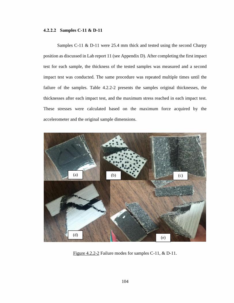
104

Samples C-11 & D-11




impact test was conducted. The same procedure was repeated multiple times until the

failure of the samples. Table 4.2.2-2 presents the samples original thicknesses, the

thicknesses after each impact test, and the maximum stress reached in each impact test.

These stresses were calculated based on the maximum force acquired by the

accelerometer and the original sample dimensions.

Figure 4.2.2-2 Failure modes for samples C-11, & D-11.

(a) (b) (c)

(d) (e)

105


11 & D-11.

After the first impact test, both samples showed some delamination in the cotton


to 3% reduction of the original thicknesses to C-11 & D-11 respectively. From the second

impact test to the sixth impact test, both samples showed more delamination failures, an

increase of the maximum stress to reach 134 MPa, and another 5% reduction in the

original thickness. Sample C-11 was tested a seventh time and the sample failed (see

Figure 4.2.2-2 a, b, &c). Sample D-11 failed after the ninth impact test and the maximum

stress reached 172 MPa (see Figure 4.2.2-2 d &e). In general, the maximum stress

increases until failure then the stress drops dramatically but the sample carries load after

failure.

Samples C-13 & D-13




Test Number

Sample C-11 Sample D-11

CDP t

(mm) Max. stress (MPa)

CDP t

(mm) Max. stress (MPa)

0 25.10 105.216 24.40 107.020

1 24.63 120.848 23.60 123.373

2 24.10 123.253 23.40 129.205

3 23.60 131.670 23.10 135.158

4 23.60 132.151 23.05 N/A

5 23.45 134.208 22.90 127.582

6 23.35 131.791 22.80 134.556

7 23.30 137.502 22.70 135.278

8 N/A N/A 22.60 136.059

9 N/A N/A 22.50 172.675

106

impact test was conducted. The same procedure was repeated ten times. For this extended

test, only ten impact tests were conducted as the stresses were not high enough to fail the

samples. Table 4.2.2-3 presents the samples original thicknesses, the thicknesses after

each impact test, and the maximum stress reached in each impact test. These stresses were

calculated based on the maximum force acquired by the accelerometer and the original

sample dimensions. For some of the tests, the accelerometer did not acquire the data.


13 & D-13.

After the first impact test, both samples showed little delamination in the cotton


reduction of the original thicknesses. From the second impact test to the last impact test,

both samples showed more delamination failures, an increase of the maximum stress to

reach 85 MPa, and another 3% reduction in the original thickness. In the last few tests,

the samples did not experience big changes in their thicknesses and the maximum stress.

In general, the maximum stress increases while the number of impacts increases.

Test Number C-13 D-13

CDP t (mm) Max. stress (MPa) CDP t (mm) Max. stress (MPa)

0 50.10 67.847 49.90 N/A

1 49.00 77.756 48.90 77.835

2 48.70 80.557 48.60 79.908

3 48.60 81.510 48.50 81.462

4 48.35 82.680 48.39 N/A

5 48.25 82.680 48.20 83.859

6 48.10 84.274 48.15 84.750

7 47.90 84.075 48.00 85.525

8 47.80 84.552 47.92 85.489

9 47.7 84.552 47.83 85.749

10 N/A N/A 47.80 85.544

107

Errors and recommendations to improve the test results

Multiple errors affected the test results. These errors are presented as follows:

The data acquired by the accelerometer had unexpected noise (see Figure 4.2.3-

1). The source of the noise could be a higher frequency mode produced by the

hammer arm low stiffness or possible baseline shift of the output data for the

accelerometer sensor (Soss 2008). This noise was reduced by adjusting the data

by taking the average of multiple consecutive data points to form a single data

point. Some of these noise errors were irrecoverable (see Figure 4.2.3-2). The

reason for these irreparable noises was the movement of the wire connecting the

accelerometer and the data acquisition system. Due to the low-quality images

acquired by the high-speed camera, some data were difficult to perform the DIC

analysis which canceled the tested specimen.

The impact test was conducted using multiple impact events so that the pendulum

impacted the samples multiple times as there were no arrest mechanism to prevent

the hammer from swinging back and impacting the specimen until the force damps

out. Figure 4.2.3-3 presents one series of impact forces exercised in one test in

terms of acceleration vs time.

Figure 4.2.3-1 Example of recoverable accelerometer data noise.

-50000

0

50000

100000

150000

0 2 4 6 8 10 12 14 16

Forc

e(N

)

Time (ms)

acc- dataadjusted-acc

108

Figure 4.2.3-2 Example of irrecoverable accelerometer data noise (high frequency and

baseline shift error).

Figure 4.2.3-3 Multiple impact events in a single impact test.

The following recommendations could prevent the errors discussed previously and

improve the test results:

-40000

-20000

0

20000

40000

60000

80000

100000

120000

140000

0 2 4 6 8 10 12

Forc

e(N

)

Time (ms)

acc-acquired

adjusted-acc

High frequency Baseline shift error

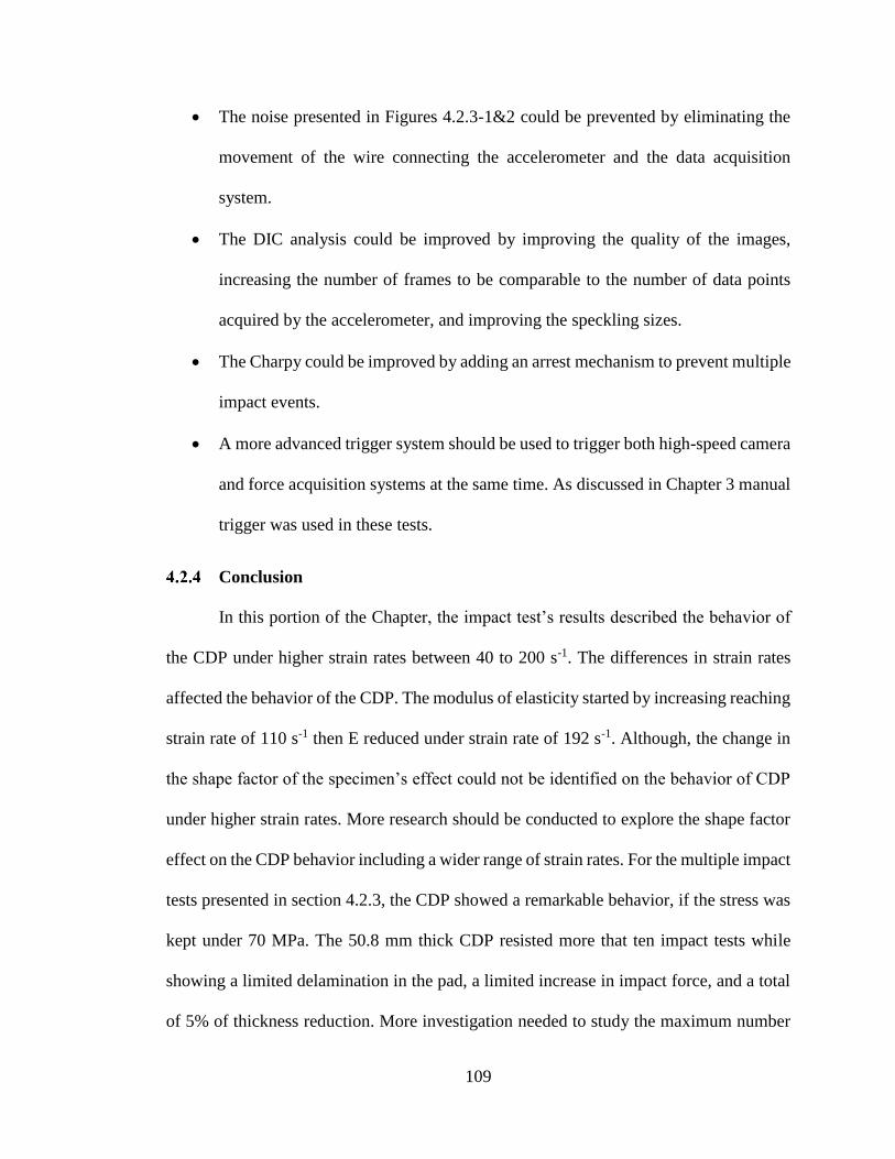
109

The noise presented in Figures 4.2.3-1&2 could be prevented by eliminating the

movement of the wire connecting the accelerometer and the data acquisition

system.

The DIC analysis could be improved by improving the quality of the images,

increasing the number of frames to be comparable to the number of data points

acquired by the accelerometer, and improving the speckling sizes.

The Charpy could be improved by adding an arrest mechanism to prevent multiple

impact events.

A more advanced trigger system should be used to trigger both high-speed camera

and force acquisition systems at the same time. As discussed in Chapter 3 manual

trigger was used in these tests.

Conclusion

In this portion of the Chapter, the impact test’s results described the behavior of

the CDP under higher strain rates between 40 to 200 s-1. The differences in strain rates

affected the behavior of the CDP. The modulus of elasticity started by increasing reaching

strain rate of 110 s-1 then E reduced under strain rate of 192 s-1. Although, the change in

the shape factor of the specimen’s effect could not be identified on the behavior of CDP

under higher strain rates. More research should be conducted to explore the shape factor

effect on the CDP behavior including a wider range of strain rates. For the multiple impact

tests presented in section 4.2.3, the CDP showed a remarkable behavior, if the stress was

kept under 70 MPa. The 50.8 mm thick CDP resisted more that ten impact tests while

showing a limited delamination in the pad, a limited increase in impact force, and a total

of 5% of thickness reduction. More investigation needed to study the maximum number

110

of impact required to fail the CDP under several stresses. The pad showed a 2% reduction

in thickness after the first test and a 2% reduction for the rest of the test, which shows that

the first impact stretched the cotton duck layers causing a sudden increase in E and a

sudden reduction in the original thickness.

Comparing static compression test results and impact test results

This Chapter reported the results for both static compression and impact tests for

CDP and described its behavior providing a general overview on the change of modulus

of elasticity while changing the strain rate. The results from both tests could be described

by the following:

The modulus of elasticity increases while increasing the strain rate (see Figure 2.3-

1). In the figure, comparing E calculated at 20 MPa, the modulus of elasticity

increased from a value of 300 MPa at strain rates 0 to 0.4 s-1 to values from 340

to 420 MPa at strain rates between 40 & 200 s-1. This increase is 15% to 40%

increase in E depending on the strain rate.

At 45 MPa, E increased from a value of 400 MPa at strain rates 0 to 0.4 s-1 to

values from 480 to 620 MPa at strain rates between 40 & 200 s-1. This increase is

20% to 55% increase in E depending on the strain rate.

At 70 MPa, E increased from a value of 600 MPa at strain rates 0 to 0.4 s-1 to

values from 700 to 780 MPa at strain rates between 40 & 200 s-1. This increase is

17% to 30% increase in E depending on the strain rate.

The maximum percentage increase in E is calculated equal to 55%.

111

Figure 4.2.4-1 E values at different strain rates calculated at 20, 45, & 70 MPa for static

and impact tests.

The following chapters used the SDOF system created in chapter 2 and the test

results presented in this chapter to build a guideline for describing the new skip slipper

design. Using E calculated from the dynamic test and the maximum stresses for CDP

provided by AASHTO Standards (20 MPa), the new skip slipper design could be designed

to reduce the bunton impact force as discussed in Chapter 2.

0

100

200

300

400

500

600

700

800

900

0 50 100 150 200

E (M

Pa)

Strain Rate (s-1)

20 MPa

45 MPa

70 MPa

static test results

112

5 Chapter 5 Developing a new slipper design

Using the dynamic analysis presented in Chapter 2, the bunton force or the impact

force and the maximum guide displacement were determined using Comro guideline or

the SDOF program. These variables are the key components to design the side slippers.

In Chapter 4, cotton duck pads (CDP) were tested under impact to be used in the new

slipper design. In this chapter, the new slipper design is developed including a design

guide based on the information presented in both chapter 2 & 4. The chapter is divided as

follows:

The current slipper design.

Developing the new slipper design using the SDOF program.

Recommendations for modifying Comro guideline.

Conclusion

Current slipper plate design

The slipper plates, presented in Comro guideline (1990) and SANS 10208:3

commentary (2001), are steel plates covered with High density polyethylene, to reduce

friction, mounted on both sides of the conveyance to carry the acting lateral loads due to

the misalignment of guides. These lateral loads can perform in two different directions:

in the plane of guides or in perpendicular to this plane (see Figure 5.1-1). The magnitude

of the lateral loads could be obtained using Comro (1990) or an equivalent SDOF program

using numerical integration of the time history as presented in Chapter 2. Using this

information, the steel could be designed to carry the impact loads without harming the

body of the conveyance (see Figure 5.1-2).

113

Figure 5.1-1: Application of lateral loads (COMMENTARY ON SANS 10208:3 –

2001)

Figure 5.1-2: Slipper plates design (COMMENTARY ON SANS 10208:3 – 2001)

These slippers do not affect the magnitude of the impact force acting on the

conveyance or the bunton, rather they transfer the load directly to the steel work without

Out of plane lateral force

In plane,

lateral force

Steel plates Bolts

s

114

harming the skip body. For extreme cases, where the bunton and skip have very high

stiffness, or the skip is moving with higher velocity, the slippers would transfer the high

impact loads directly to the skip and the bunton which increases the steelwork needed to

carry these large impact forces.

A material with less stiffness could be used in the slipper design to reduce these

extreme impact forces by decreasing the stiffness of the system. The new slipper design,

presented in this chapter, uses elastomer pads as a cushion to change the dynamic

properties of the system, reduce the impact force and transfer a smaller portion of force

and displacement to the skip and bunton system.

The new slipper design using the SDOF Newmark’s method

The new slipper design is based on creating a lower effective bunton stiffness by

adding an elastomer pad with low stiffness to the effective bunton stiffness in series (see

Figure 5.2-1). The final effective stiffness can be calculated by adding the pad stiffness to

the original effective stiffness in series as presented in Equation 5-1.

Figure 5.2-1: The addition of the elastomer pad stiffness to the SDOF system presented

in chapter 2 to form a new SDOF system.

me me

kp k

p k

be k

be

+ =

115

𝑘𝑝𝑏𝑒 =𝑘𝑏𝑒𝑘𝑝

𝑘𝑏𝑒+𝑘𝑝 Equation 5-1

where: 𝑘𝑏𝑒 is the effective bunton stiffness, 𝑘𝑝 is the elastomer pad stiffness, and 𝑘𝑝𝑏𝑒 is

the combined effective stiffness.

In this research, CDPs are recommended due to its higher overall compressive

strength compared to plain unreinforced elastomeric pads (PEP), Fiberglass-Reinforced

Pad (FGR), and Steel-Reinforced Elastomeric Bearing. The CDPs were tested under

impact force as presented in chapter 3 &4. The results of these tests were as follows:

The stress-strain curve for impact is presented as a second-degree polynomial

curve regression.

The modulus of elasticity was calculated by dividing the stress equation by strain

and a secant value of E at each strain (see Table 5.2.1-1).

The dynamic amplification factor, comparing the static and dynamic test, was

found equal to a maximum of 50% of the static compressive modulus of elasticity.

Under impact loads, the CDP carried ten impacts of stress 70 MPa up to 85 MPa

without showing any failure.

Using the results shown above, the SDOF program, created in chapter 2, can be

used to obtain a new dynamic response including the calculating the maximum bunton

force. Two methods were used in calculating the pad stiffness and using Equation 5-1 to

calculate the new effective stiffness:

The CDP stiffness function obtained by multiplying the pad modulus of

elasticity’s function (𝐸𝑝) by the ratio between the pad area (A) and thickness (t)

(see Equation 5-2).

116

𝑘𝑝 =𝐸𝑝 𝐴

𝑡 Equation 5-2

To facilitate the design procedures, constant value for 𝐸𝑝 (E*) can be calculated

using conservation of energy method, where the area under the pad stress-strain

curve is equal to the area under the curve created by a constant value E* at a given

stress value.

Calculating the maximum bunton force and displacement using EP

Table 5.2.1-1 presents the modulus of elasticity equations created for each

dynamic test performed in chapter 4. Using Equation 5-2, 𝑘𝑝 functions were calculated

by the Ep functions presented in the table.

Table 5.2-1: 𝐸𝑝 modulus of elasticity and pad stiffness 𝑘𝑝 based on secant calculations,

where u is the pad displacement and t is the pad thickness.

Test

number

Modulus of elasticity equation

(𝐸𝑝) (MPa) Pad Stiffness 𝑘𝑝 (N/m)

8 2144.5ε + 16.57 (2.145x109 𝑢

𝑡 + 16.57 x106)

𝐴

𝑡

9 1869.7ε - 5.38 (1.870 x109 𝑢

𝑡 - 5.38 x106)

𝐴

𝑡

10 1674.9ε - 10.47 (1.675x109 𝑢

𝑡 - 10.47 x106)

𝐴

𝑡

11 1967.0ε - 11.56 (1.967x109 𝑢

𝑡 - 11.56 x106)

𝐴

𝑡

12 1845.8ε + 23.15 (1.846x109 𝑢

𝑡 + 23.15 x106)

𝐴

𝑡

13 1306.4ε + 95.02 (1.306x109 𝑢

𝑡 + 95.02 x106)

𝐴

𝑡

Average 1984.5ε - 15.45 (1984.5x109 𝑢

𝑡 - 15.45 x106)

𝐴

𝑡

The 𝑘𝑝 functions were used in the numerical integration spreadsheet presented in

Chapter 2 to evaluate the effect of adding 𝑘𝑝 in series to the bunton effective stiffness in

117

the example staged in Appendix A. The elastomer bearing pad stiffness (𝑘𝑝) was

calculated for every time step by using the previous step pad displacement (up) as shown

in Equation 5-3.

𝑘𝑝+1 =C1 up +C2 Equation 5-3

where 𝑘𝑝+1 is the pad stiffness at a certain time step, C1 & C2 are constants depending on

the area and thickness of the CDP the equation used from Table 5.2.1-1, up is the pad

displacement in the previous time step. up was calculating using the following equation:

𝑢𝑝 =ui - ube Equation 5-4

where ui is the total displacement of the system and ube is the displacement obtained by

dividing the bunton force by the effective bunton stiffness at each time step.

Multiple trials were performed while changing the area and thickness of the CDP

used to reduce the bunton force and guide displacement. For the example presented in

Appendix A, a pad with the same size as the side slippers (500 mm × 200 mm) was used

(see Figure 5.2-2). This pad size resulted in a negligible reduction in the impact force as

the stiffness of the pad was relatively high (see Figure 5.2-4). After multiple trials, the

most practical solution to reduce the area of the CDP without affecting the size of the

slippers was by using CDP washers at the bolts locations of the original slippers (see

Figure 5.2-2). The washer sizes and number could be determined by calculating the

maximum impact force expected to be carried by the pad using the numerical integration

spreadsheet, as presented in Chapter 2, or by using Comro guideline and the maximum

allowable stress that the CDP could carry. The allowable compressive stress, provided by

ASSHTOO 2012, is 3 ksi (20.3MPa). This allowable stress could be increased to 35 MPa,

118

as the impact events are rare to happen with the calculated magnitude. Also, The CDP

could carry stress 70 MPa in impact without failure as presented in the test results chapter

4. It is recommended to use washer sizes provided by the manufactures.

Figure 5.2-2: CDP mounted between the slipper plate and the skip (Pad and washer

forms).

To study the effect of changing the pad size on the bunton force and the bunton

displacement, the following graphs (Figure 5.2-3&4) were created using the mine

information provided in Appendix A and adding CDPs in series to the effective bunton

stiffness while changing the thicknesses and the areas of the pads.

Comparing the results of adding the CDP to the system, the following was found:

Reducing the area and increasing the thickness of the pad decreases the total pad

stiffness which reduces the bunton force.

In this example, the pad stiffness had to be reduced considerably to show a

significant effect on the bunton force. Using lager areas and smaller pad thickness

Washers

CDP

119

was not effective. On the other hand, using washers with smaller area and larger

thickness reduced the impact force.

The percent reduction in bunton displacement was equivalent to the percent

reduction in bunton force with a maximum of 38% reduction using six CDP

washers of total area equal to 821 mm2 and thickness equal to 50.8 mm (see Figure

5.2-4). The maximum stress of these washers was 15.2 MPa.

In figure 5.2-3&4: fp is the bunton force while the CDP is mounted to the slipper

and fb is the bunton force without CDP.

Figure 5.2-3 Ratio between the bunton forces before and after adding CDP compared by

different pad thicknesses with the same area (821mm2).

0.0

0.1

0.2

0.3

0.4

0.5

0.6

0.7

0.8

0.9

1.0

0 10 20 30 40 50 60

f p/f

b

Pad thickness (mm)

fp/fb Vs. Padthickness

fp = 21 kN

120

Figure 5.2-4 Ratio between the bunton forces before and after adding CDP compared by

different pad areas with the same pad thickness (50.8 mm).

The data presented previously shows the effect of the CDP on the behaviour of the

SDOF system with non-linear elastomer pad stiffness. The stiffness of the pad is desirable

to be smaller than the effective bunton stiffness to significantly reduce the bunton force.

Using a function to calculate the CDP stiffness is impractical. A single value of modulus

of elasticity is needed to simplify the design process for the mine steelwork. The following

section describes the equivalent secant value of modulus of elasticity (E*) using

conservation of energy method.

Calculating the maximum bunton force and displacement using secant value

of modulus of elasticity (E*)

It is common to convert a non-linear behaviour of a certain material (concrete for

example) to a linear equivalent behaviour to simplify the design procedures. One of the

common methods used to transform the non-linear material behaviour to an equivalent

0.0

0.2

0.4

0.6

0.8

1.0

1.2

0.00 0.02 0.04 0.06 0.08 0.10 0.12

f p/f

b

Ap (m2)

Fp/Fb Vs. Ap

fp = 21 kN

A=(100,000mm2)

A=(821mm2)

121

linear behaviour is conservation of energy. The energy absorbed by the pad was calculated

using integration of the polynomial equation to calculate the area under the stress-strain

curve up to the maximum allowable stresses: 20 MPa by ASHTOO 2012 and the

recommended allowable stress 35 MPa. Two values of E* were calculated for each

allowable stress. Each value of E* could be used to calculate the maximum bunton force

and the maximum skip displacement. Figure 5.2-5 presents two values for E*, calculated

to be equivalent to the nonlinear behaviour up to 20 MPa allowable stress, 300 MPa to

calculate the maximum skip displacement and bunton force and 150 MPa to calculate the

maximum pad deflection. Figure 5.2-6 presents two values for E*, calculated to be

equivalent to the nonlinear behaviour up to 35 MPa allowable stress, 400 MPa to calculate

the maximum skip displacement and bunton force and 200 MPa to calculate the maximum

pad deflection. The area under the curves created by the E* values are equal to the area

under the actual stress-strain curve of CDP while maintaining the same maximum stress

(20 or 35 MPa) or maximum strain.

122

Figure 5.2-5: Actual stress-strain curve of CDP and the curves created by the equivalent

values of E* for 20 MPa allowable stress.

Figure 5.2-6 Actual stress-strain curve of CDP and the curves created by the equivalent

values of E* for 35 MPa allowable stress.

0

5

10

15

20

25

0.00 0.02 0.04 0.06 0.08 0.10

Stre

ss (

MP

a)

Strain (mm/mm)

Stress-strain curve

Constant E-maximum σ

Constant E - maximum ε

0

5

10

15

20

25

30

35

40

0 0.02 0.04 0.06 0.08 0.1 0.12 0.14

Stre

ss (

MP

a)

Strain (mm/mm)

Stress-strain curve

Constant E - maximum σ

Constant E - maximum ε

123

E* values are then used to calculate 𝑘𝑝 using Equation 5-2 which is then used to

calculate 𝑘𝑝𝑏𝑒 using Equation 5-1. The new effective bunton stiffness could be then used

to perform the dynamic analysis to calculate the maximum bunton force and maximum

skip displacement. It is recommended to use the E* equivelant for the purpose of the

analysis, bunton force or skip displacement.

Both non-linear Ep and E* were compared using the SDOF integration spreadsheet

and the results were equivelant depending on the value of the maximum stress. E* was

then used to calculate the new effective bunton stiffness which later is used in calculating

the maximum bunton force or skip displacement using Comro guideline.

The new slipper design using Comro guideline

The slipper design using Comro guideline could be performed as follows:

Calculate the bunton force and skip displacement using SANS 10208-4: (2011).

In this step, the bunton force and skip displacement should be calculated using the original

information of the skip system. Including the effective mass and stiffness, the velocity

and the maximum guide misalignment.

Calculate the new rubber slipper area needed using the bunton force and a

maximum allowable stress selected (20 or 35 MPa), using Equation 5-5:

𝐴 =𝐹𝑏

20 𝑜𝑟 35 𝑀𝑃𝑎 Equation 5-5

Select pad thickness based on the available space between the guide and slipper

and calculate 𝑘𝑝 using E* values depending on the response needed to be tested. In other

words, calculate two different 𝑘𝑝 one used to calculate the maximum new bunton force

and skip displacement and the other used to calculate maximum pad deflection.

124

Calculate new 𝑘𝑝𝑏𝑒 including 𝑘𝑝 as a stiffness in series (Equation 5-1).

Calculate the new bunton force & guide displacement using SANS 10208-4

(2011) and the new 𝑘𝑝𝑏𝑒.

Design steel work.

The following flow chart describes the steps needed to complete the slipper design

and the new steel work design based on the new bunton forces and skip displacement.

Using this procedure, the design results were comparable to the results using

integration spreadsheet applying non-linear and linear systems. Table 5.3-1 presents the

design of the CDP using the methods previously discussed in this chapter.

125

Figure 5.3-1: Flowchart for the new slipper design.

Calculate the bunton force & guide

displacement using COMRO (1990)

Designing the new slipper

Design steel work

Calculate the new rubber slipper

area 𝐴 =𝐹𝑏

20 𝑜𝑟 35 𝑀𝑃𝑎 and pick CDP

thickness

Calculate 𝑘𝑝 =𝐸∗ 𝐴

𝑡

Calculate the new bunton force

& guide displacement using

Comro 1990 & 𝑘𝑝𝑏𝑒

σ = 35 MPa σ = 20 MPa

E* = 300 MPa

(skip displacement &

Bunton force)

E* = 400 MPa

(skip displacement &

Bunton force)

Calculate 𝑘𝑝𝑏𝑒 =𝑘𝑏𝑒𝑘𝑝

𝑘𝑏𝑒+𝑘𝑝

126

Table 5.3-1: SDOF integration Spreadsheet results for bunton force, skip displacement,

pad stress & pad deflection (for skip without pad and with 6 washers using Ep function

and the equivalent E*) and the results using Comro guideline for the same washer sizes.

Input

impact velocity (v) 0.05 m/s Washer Area 0.21 in2

Time step (Δt) 0.0015 sec Washer # 6 Effective mass (me) 23721.15 kg Ap 0.000821 m2

Bunton Stiffness (kb) 26820000 N/m

Pad thickness (Tp) 50.8 mm

Skip Stiffness (ks) 9100000 N/m

Output

Without

Pad

Comro (1990) E*=300

Washer (MPa)

Ep E*=150 E*=300

Force (N) 20066 13046 12718 10292 12952

Stress (Mpa) N/A 15.897 15.497 12.541 15.783

Skip displacement (m) 0.0030 0.0050 0.0020 0.0015 0.0019

Pad deflection (m) N/A 0.0043 0.0042 0.0375

In Table 5.3-1, the results of using the Ep function and E*=300 MPa in the

dynamic analysis and using SANS 10208-4 (2011) guideline were similar in maximum

bunton force and maximum pad stress. The results were similar for the pad deflection

between using Ep function and E*=150 MPa. The Skip displacement was similar for Ep

function and E*=300 MPa. the total deflections of the system using SANS 10208-4

(2011) and E*=150 MPa are equivalent.

Conclusion

In this chapter, the new slipper design was introduced. Using the information on

CDP, tested in Chapter 3& 4, a pad was used between the slipper’s steel plate and skip to

create a lower effective stiffness and reduce the bunton force. This pad stiffness was tested

127

using SDOF integration spreadsheet for non-linear behavior and the equivalent linear

behaviour. The results using both behaviours were similar. A guideline was introduced to

use the new slipper design and Comro guideline to calculate the maximum bunton

stiffness and skip displacement to design the mine steelwork.

128

6 Chapter 6 Conclusion

Conclusions

This research was conducted to improve the skip side slippers design. The new

slipper design provides information about how to reduce slam loads in mineshafts of deep

mines. Slam loads are highest when there is steel-to-steel contact between the slippers and

the shaft rails. This hard contact has the most harmful effect on the steelwork of the

mineshaft. The slam load is primarily influenced by the following:

Misalignment of the shaft guide.

The bunton, skip, and guide stiffness.

The mass of the skip and the hoisting velocity.

The worst-case scenario for slam loads has a combination of high stiffness buntons

and skips with high velocity hoisting along with high mass skips. In extreme cases, the

mass of the skip may be up to 130 tonnes and the hoist speed up to 18m/s.

To increase the productivity of a mine, the mass and the velocity of the skip should

be maximized. A high mass and high velocity system could result in high slam loads,

requiring stronger steelwork for the mineshaft. This would likely also result in a stiffer

mineshaft rail system, which has the effect of further increasing potential slam loads. An

alternative to increasing capacity of the rails is to reduce the effective stiffness of the

skip/guide system. This reduction in stiffness will reduce the maximum bunton force. One

way to reduce stiffness is to provide an additional flexible material at the slipper location

that acts in series with the skip and rail system. This flexible slipper reduces the effective

bunton stiffness and therefore the bunton impact force.

129

Cotton Duck Pads (CDP), used as bearing pads in multiple applications, were

tested to examine their behavior under static and dynamic compression loads. Chapter 4

reported the results for both types of tests for CDP and described the material with a focus

on the change of modulus of elasticity with changing the strain rate. The results from both

tests are described by the following:

As expected, the modulus of elasticity increases with increasing the strain rate.

The modulus of elasticity can be represented by a second-degree polynomial

curve.

CDP carries multiple impacts, with stresses between 70 and 85 MPa, without

showing any noticeable failure.

The maximum amplification factor of the modulus of elasticity due to high strain

rate was found equal to 50%.

Using the results of the tests performed on CDP, the new slipper design was

created using CDP between the slipper’s steel plate and the skip body. This new system

reduced the effective bunton stiffness which reduced the maximum bunton force. To

facilitate the new design procedures, a constant modulus of elasticity (E*) was introduced

to create a linear system instead of a non-linear system represented by a second-degree

polynomial equation. Two limits for the maximum stress of CDP were introduced: the

maximum allowable stress provided by AASHTO Standards (20 MPa) and a suggested

maximum allowable stress based on the conducted tests (35 MPa). The designer has the

choice to select any of these two values. The designer starts by finding the maximum

bunton force from the analysis of the original system using SANS 10208-4 (2011). Using

the calculated maximum force and maximum allowable stress, allows the designer to

130

select the area of the pad needed to keep the pad stress level below the allowable stress

limit. Then, a pad thickness is selected depending on the allowed distance between the

slipper plate and the guide surface. The pad stiffness (kp) is calculated using the pad area

and thickness previously obtained and E* value: 300 MPa for the stress of 20 MPa and

400 MPa for the stress of 35 MPa. A new effective bunton stiffness is then calculated and

a new bunton force is obtained using SANS 10208-4 (2011). The results of this method

were compared to the results of using numerical integration of time history for a single

degree of freedom system while using the non-linear pad behavior.

Suggestions for further research

This thesis provided a theoretical study for a new slipper design methodology.

Further research needed could be presented as follows:

Mount the new slipper of the side of an actual skip to compare the real-life force

magnitude with the theoretically calculated bunton force.

Test CDP for fatigue to measure the life span for this pad using the stress limits

discussed in this thesis.

Test more CDP sizes under static loading and impact to improve the understanding

of the CDP behavior.

Test more CDP samples while examining the temperature effect on its behavior

using different loading rates.

131

References

- American Association of State Highway and Transportation Officials.

(2012). AASHTO LRFD bridge design specifications. Washington, D.C: American

Association of State Highway and Transportation Officials.

- Biggs, J.M. (1964) Structural Dynamics. McGraw-Hill Book Company, USA

- Chamber of Mines Research Organization (COMRO). User Guide No. 21:

Design guidelines for thedynamic performance of shaft steelwork and conveyances.

Auckland Park: COMRO. 1990.

- Chopra A.K. (2006), Dynamics of structures: Theory and applications to

earthquake engineering, 3rd ed.

- Cloth, Duck, cotton or cotton-polyester blend, synthetic rubber, impregnated

and laminated, oil resistant (1989) MIL-C-882E

- Commentary on SABS 0208:4 – 1st ed (2001), The design of structure for the

mining industry part 4 – Shaft System Structures - Krige G.J. - Southern African Institute

of Steel Construction.

- Gent, A. N. (1958). On the Relation between Indentation Hardness and Young's

Modulus. Rubber Chemistry and Technology, 31Laboratory Evaluation of Full Size

Elastomeric Bridge Bearing Pads (4), 896-906.

- Krige G. J. (May 1983), Thesis: The Behaviour and Design of Mineshaft

steelwork and conveyances. University of the Witwatersrand, Johannesburg, South

Africa.

- Krige G. J. (Jun 1986), Some initial findings on the behaviour and design of

mine-shaft steelwork and conveyances journal of the south African institute of mining

and metallurgy. vol. 86. no. 6. Jun. 1986. pp. 205-215.

- Robert H. Bishop (2015), Learning with Labview.

- Lehman, D. E., C. W. Roeder, R. Larson, and K. Curtin. (2003). Cotton Duck

Bearing Pads: Engineering Evaluation and Design Recommendations, Research Report

No. WA-RD 569.1. Washington State Department of Transportation, Olympia, WA.

- Lehman, D. E., Roeder, C.W., Larsen, R.A. (2005) Design of cotton duck bridge

bearing pads Journal of Bridge Engineering, 10 (5), pp. 555-563.

-National Instrument (NI): Measuring Strain with Strain Gages. Publish

Date: May 25, 2016.

- NCORR v1.2 Open source 2D-DIC Matlab Sofware.

- Roeder, C. W., and J. F. Stanton. 1983. “Elastomeric Bearings: A State of the

Art,” Journal of the Structural Division. American Society of Civil Engineers, New York,

NY, Vol. 109, No. 12, December 1983, pp. 2853–2871.

https://www-scopus-com.proxy.hil.unb.ca/record/display.uri?eid=2-s2.0-24944458178&origin=reflist&sort=plf-f&cite=2-s2.0-24944458178&src=s&imp=t&sid=73d477b17bb2cd218ff3a9c9755d0dfe&sot=cite&sdt=a&sl=0&recordRank=

https://www-scopus-com.proxy.hil.unb.ca/record/display.uri?eid=2-s2.0-24944458178&origin=reflist&sort=plf-f&cite=2-s2.0-24944458178&src=s&imp=t&sid=73d477b17bb2cd218ff3a9c9755d0dfe&sot=cite&sdt=a&sl=0&recordRank=

132

- Roeder, C. W., and J. F. Stanton. (1986). “Failure Modes of Elastomeric Bearings

and Influence of Manufacturing Methods.” In Vol. 1, Proc. of 2nd World Congress on

Bearings and Sealants, Publication SP-94-17. 84-AB. American Concrete Institute,

Farmington Hills, MI.

- Roeder, C. W. (1999). “LRFD design criteria for cotton duck pad _CDP_ bridge

bearing.” Final Rep. on NCHRP Project 20-07/99, National Cooperative Highway

Research Program, Transportation Research Board, National Research Council,

Washington, D.C.

- Stantec (2013), Shaft Steel Testing- Sample No 1 Typical set – Plan & Details,

Drawing No: D-JANSEN_ 2616_SK 0001, Saskatchewan, Canada.

- Stanton, J. F., and Roeder, C. W., (1982) "Elastomeric Bearings—Design,

Construction and Materials," NCHRP Report 248, Sept., 1982.

- Soss D.A., (2008) Method for determining when a force sensor signal baseline

in a force-based input device can be updated, U.S. Patent 20080167832, July 10, 2008.

- South African National Standard, Design of structures for the mining industry

part 4: Shat system structures SANS 10208-4 (2011).

133

Appendix

134

A Example for calculating the bunton force using Comro (1990)

A.1 General information

Shaft configuration (see Figure A.1-1).

Shaft maintenance classification: C (default for design) (e= 20 mm)

Buntons : HSS 203 x 203 x16

Guides : HSS 203 x 203 x16

Conveyances: Compartments A1 and A2 – 22T Skip

Compartments B1 – Balancing weight

Compartments C1 – man cage

Bunton Spacing: 8 m

Hoisting speed: 10 m/s

Conveyance Data: Skip A1 (22.6 x 1.85 x 1.65)

Full mass: 94,400 kg

Empty mass: 42,400 kg

Stiffness (ks): 9.1 KN/mm

Distance of skip c.g. from slipper plate: 11.3 m

Moment of inertia about global Z axis: 4.19 x106 kg m2

135

Figure A.1-1 Mineshaft plan view configuration

A.2 Shaft steelwork design

Steelwork stiffness: kg= 2.49 x 106 N/m

kb= 26.82 x 106 N/m

But the skip is flexible ks = 9.1 KN/mm

Bunton effective stiffness kbe = 𝑘𝑏𝑘𝑠

(𝑘𝑏+𝑘𝑠)

=26.82 𝑥 106 𝑥 9.1 𝑥 106

26.82𝑥 106 + 9.1 𝑥 106

kbe = 6.79 x 106 N/m

Effect mass 𝑚𝑒 =𝑚𝑠𝐼

(𝐼+𝑚𝑠ℎ2)

B1

C1

A2 A1

136

= 94,400 𝑥 4.19 𝑥 106

4.19 𝑥 106 + 94,400(11.6)2

𝑚𝑒= 23,721.15 kg

Stiffness ratio rk = 𝑘𝑏𝑒

𝑘𝑔

= 6.79 𝑥 106

2.49 𝑥 106

rk = 2.72

Note: 𝑘𝑏𝑒 is used instead of 𝑘𝑏 because the skip is flexible.

Impact velocity ratio 𝑢

𝑣 =

2𝑒

𝐿

= 2(0.02)

8 = 0.005

𝑘𝑏 : nondimensional steelwork stiffness at bunton

𝑘𝑏 =

𝑘𝑏𝑒𝐿2

𝑚𝑒𝑣2

= 6.79 𝑥 106𝑥 82

23,721.15 𝑥 102 = 183.2

Using the figures provided in Comro 1990 (Figure A.2-1 to A.2-4), the following was

determined:

Ratio of rebound velocity to the impact velocity u (ru)

ru = 1.3

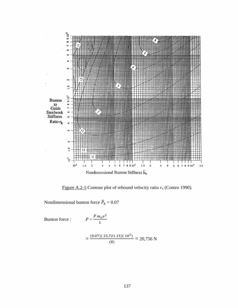
137

Figure A.2-1:Contour plot of rebound velocity ratio ru (Comro 1990).

Nondimensional bunton force 𝑏 = 0.07

Bunton force : P = 𝑃 𝑚𝑒𝑣2

𝐿

= (0.07)( 23,721.15)( 102)

(8) = 20,756 N

138

Figure A.2-2: Contour plot of nondimensional bunton force 𝑃𝑏 for u/v = 0.005 (Comro

1990).

Non-dimensional guide displacement 𝛿 = 0.000667

Guide displacement 𝛿𝑠 = 𝛿 𝐿 = (0.000667) (8) = 0.00533 m

139

Figure A.2-3: Contour plot of nondimentional skip displacement 𝛿 for u/v = 0.005

(Comro 1990).

Nondimentional guide bending moment = 0.011

Guide bending moment M = 𝑚𝑒𝑣2

= (0.011) (23,721.15) (102) = 26,093.265 N.m

140

Figure A.2-4: Contour plot of nondimentional guide bending moment for u/v =0.005

(Comro 1990).

141

B Data acquisition systems

B.1 Data acquisition system for accelerometer and load cell

The data acquisition system was used to acquire the forces, applied force measured

using the accelerometer and the reaction force measured by the load cell. The impact event

data was transmitted from the accelerometer and load cell as an electrical current to

National Instrument Analog input cards. Two types of cards were used: NI 9205 and NI

9237.

- NI 9205 contains 16 Differential Analog Input channels. It could acquire ± 200

mV and up to ± 10 V. The maximum number samples acquired per second is

250,000 samples. This card was used to acquire the change in voltage in the

accelerometer.

- NI 9237 is used to acquire Bridge Analog Input. It has a half- and full-bridge

measurements built-in. The Card could acquire signals of ± 25mV/V and a

maximum number of samples of 50,000 samples/second/channel. This card was

used to measure the output voltage of the load cell.

The two cards were connected in series using the model NI cDAQ-9172 series C

which helped acquiring data from both cards using the onboard clock at the same time

intervals. The model was then connected to a computer using a high-speed USB 2. The

computer was equipped with a software (Labview) providing control and access the model

data including triggering the test, acquiring data in a tabulated form, and stopping the

test.More details about building the Labview program and National Instruments

equipment would be found in Labview help and NI guidelines.

142

B.2 Data acquisition system for displacement

The data acquisition system used for acquiring the deflection of the rubber

specimen. This system consists of two stages; recording the frames captured by the high-

speed camera during the impact event for every rubber sample and digital image

correlation program to analyze the deflection of the rubber. A computer software (Photon

FastCam Viewer ver 2) was used to record the frames needed. This software could be

used to adjust the frame rate, shutter rate, image resolution, trigger the image recording,

stop the record, and save the captured images in different formats (images or video

extensions) (see Figure B.2-1). The images recorded by the camera and Photron FastCam

viewer ver 2 was used in the DIC analysis.

Figure B.2-1: Photron FastCam viewer ver 2 used to record the high-speed camera’s

images.

143

The digital image correlation (DIC) was conducted using an open source 2D-DIC

Matlab Sofware NCORR V2. The following are the steps used to complete the DIC

analysis using the NCORR V2 program:

(a) After capturing the images using the high-speed camera, the speckled images were

recorded on the program as a reference image (the first recorded image before the

impact event) and the impact event recorded images (see Figure B.2-2).

(b) Drawing the region of interest: In this step, to reduce the analysis time, an area of

interest is defined to specify the area of the image where the DIC should be

performed (see Figure B.2-3).

Reference

image

Impact event

images

Figure B.2-2: The reference image and the impact event images.

144

(c) Performing the DIC analysis: In this step, the program performs the analysis based

on multiple parameters as: number of seeds, the greyscale level of the pixel picked

for the analysis, and relating the images using step analysis. The product of this

step is determining the movement of each pixel picked for the analysis through

the entire series of images in terms of pixels.

(d) After determining the movement of each pixel in the region of interest in pixel

units, the pixels’ displacements were transformed to mm units using unit

conversion tool. The unit conversion tool performs by defining a measured

distance on the image, typically the thickness of sample before the test, to

determine the number of pixels in one mm distance (see Figure B.2-4).

Figure B.2-3: Drawing region of interest

145

The result of the DIC analysis is presented in an array form of pixel displacements

for each image in the region of interest (see Figure B.2-5). An average value of

displacement was calculated for the most deflected column or row of pixel displacement

values. As previously discussed, this method was used in the static compression test to be

compared to the LVDTs’ data and ensure the accuracy of the method including the speckle

size, resolution of the images, and the frame rate used.

Figure B.2-4: Identifying the unit conversion factor

146

More details about the DIC method used to acquire the displacement is found in

the NCORR guidelines.

image

number

The column

used to

determine the

maximum

deflection

Figure B.2-5: Matlab Array of pixel displacements for image 23.

147

C Lab reports for static testing

148

Strain Rate and Stress-Strain Plots Sample A-1:

C.1 Lab report 1

12.5

mm

Date of test: December 13th, 2016.

Testing machine: Universal

compression testing machine (UCTM).

Specimen Dimensions:

Figure C.1-1: Specimen Dimensions

Material Type: Cotton Duck Pad

Number of Specimens: 4

Test Type: Compression

Loading Rate: 12 mm/min

Experimental Set up:

Descriptive notes:

The specimen was cut into the

specified dimension using a band saw

(see Figure C.1-1).

The specimen was centered inside

the UCTM to maintain a well

distributed load (see Figure C.1-2).

The specimen was centered between

the two LVDTs to maintain an

accurate deflection recording.

The LVDTs are mounted on the

steel plate that was used to distribute

the load to the specimen.

The loading rate was specified using

the computer program associated with

the machine.

The machine is also equipped with a

load cell with a capacity of 250 KN.

The data from the load cell and the 2

LVDTs were recorded using the same

computer program.

A maximum displacement of 5 mm

was set for the moving head to

prevent overloading.

Non-moving bottom

Moving

head

With load

Specimen

2 LVDTS 40 mm

cm

Steel

plate

Figure C.1-2: (UCTM) set up.

Figure C.1-3: Strain rates from 2 LVDT

and their average for sample A-1

Figure C.1-4: Stress-strain curves for 2

LVDTs and their average for sample A-1

0.00

0.05

0.10

0.15

0.20

0.25

0.30

0.35

0.40

0 10 20 30

Stra

in (

mm

/mm

)

Time (sec)

Strain-1-A-1Strain-2-A-1Average

0

20

40

60

80

100

120

0 0.1 0.2 0.3

Stre

ss (

MP

a)

Strain (mm/mm)

LVDT1-A-1

LVDT2-A-1

Average

12.5

mm

149

Stress-strain curve for all four samples and average:



0

20

40

60

80

100

120

0.00 0.05 0.10 0.15 0.20 0.25 0.30 0.35 0.40

Stre

ss (

MP

a)

Strain (mm/mm)

S-1-AverageS-A-1S-B-1S-C-1S-D-1

Observations and Discussion:

The stiffness of the rubber increases while the applied load increases. The

stress-strain relation is a non-linear relationship.

The strain rate, shown as slope in Figure C.1-3, was relatively constant

over the duration of the test due to the constant specified displacement

base load rate. The average LVDT calculated strain rate = 14.1×10-3 s-1.

An average displacement was calculated from the data provided by the two

LVDTs (see Figures C.1-3&4).

The average stress-strain data will be then used to be compared with other

strain rates and other rubber thicknesses.

The provided Stress-strain curves, in Figure C.1-5, are calculated using the

measured dimensions of each sample as specified in Table 4.1-1. Table

C.1-1 shows calculated Stresses and strains of all four samples.


calculated based on the measured dimensions of each sample.

Stress (MPa) Strain:0.05 Strain:0.10 Strain:0.20 Strain:0.30

Stress: A -1 3.567 11.136 22.902 79.207

Stress: B -1 4.275 12.815 29.362 88.172

Stress: C -1 5.263 15.410 44.718 100.040

Stress: D -1 2.519 11.497 41.591 97.276

150


C.2 Lab report 2

12.5

mm

0

20

40

60

80

100

0 0.1 0.2 0.3

Stre

ss (

MP

a)

Strain (mm/mm)

LVDT1-A-2LVDT2-A-2Average











Descriptive notes:



(see Figure C.2-1).












the machine.





computer program.




Non-moving bottom

Moving

head

With load

Specimen

2 LVDTS 40

cm

Steel

plate



and their average for sample A-2 Figure C.2-4: Stress-strain curves for 2


0.00

0.05

0.10

0.15

0.20

0.25

0.30

0.00 1.00 2.00 3.00 4.00

Stra

in (

mm

/mm

)

Time (sec)

Strain-1-A-2

Strain-2-A-2

Average

12.5

mm

151




0

10

20

30

40

50

60

70

80

90

100

0.00 0.05 0.10 0.15 0.20 0.25 0.30

Stre

ss (

MP

a)

Strain (mm/mm)



The stiffness of the rubber increased while increasing the applied force.



base load rate. The average LVDT calculated strain rate =79.7 ×10-3 s-1.



In Figure C.2-5, the stress-strain curve for samples B-2 & D-2 had

unexpectedly stopped, as the moving head started applying the force after

moving 1 or 2 mm without applying any load.







Stress: A -2 6.569 18.077 50.403 64.243

Stress: B -2 5.331 17.386 52.698 67.983

Stress: C -2 3.502 15.359 49.420 64.021

Stress: D-2 4.927 14.204 50.064 62.216

152


C.3 Lab report 3

12.5

mm

0

20

40

60

80

100

120

0 0.1 0.2 0.3

Stre

ss (

MP

a)

Strain (mm/mm)

LVDT1-A-3

LVDT2-A-3

Average











Descriptive notes:



(see Figure C.3-1).

The specimen was centered inside the

UCTM to maintain a well distributed

load (see Figure C.3-2).




The LVDTs are mounted on the steel

plate that was used to distribute the

load to the specimen.



the machine.





computer program.




Non-moving bottom

Moving

head

With load

Specimen

2 LVDTS 40mm

cm

Steel

plate






0.00

0.05

0.10

0.15

0.20

0.25

0.30

0.35

0.0 0.5 1.0 1.5

Stra

in (

mm

/mm

)

Time (sec)


12.5

mm

153




0

20

40

60

80

100

120

0.00 0.05 0.10 0.15 0.20 0.25 0.30

Stre

ss (

MP

a)

Strain (mm/mm)



The stiffness of the rubber increases while the applied load increases.



base load rate. The average LVDT calculated strain rate = 202.8 ×10-3 s-1.



In Figure C.3-5, the stress-strain curve for samples B-3 & D-3 had

unexpectedly stopped, as the moving head started applying the force after

moving 1 or 2 mm without applying any load.







Stress: A -3 4.817 16.753 51.354 66.414

Stress: B -3 3.609 14.574 48.724 62.933

Stress: C -3 4.483 15.766 50.877 65.669

Stress: D -3 3.875 14.891 49.331 63.836

154


C.4 Lab report 4

12.5

mm

0

20

40

60

80

100

120

0 0.1 0.2 0.3

Stre

ss (

MP

a)

Strain (mm/mm)












Descriptive notes:



(see Figure C.4-1).

The specimen was centered inside the

UCTM to maintain a well distributed

load (see Figure C.4-2).




The LVDTs are mounted on the steel

plate that was used to distribute the

load to the specimen.



the machine.





computer program.

A maximum Load of 160 KN was set

for the moving head to prevent

overloading.

Non-moving bottom

Moving

head

With load

Specimen

2 LVDTS 40

cm

Steel

plate





0.00

0.10

0.20

0.30

0.40

0 0.2 0.4 0.6 0.8

Stra

in (

mm

/mm

)

Time (sec)

Strain-1-A-4

Strain-2-A-4

Average

12.5

mm

155




0

20

40

60

80

100

120

0.00 0.05 0.10 0.15 0.20 0.25 0.30 0.35

Stre

ss (

MP

a)

Strain (mm/mm)

S-4-Average

S-A-4

S-B-4

S-C-4

S-D-4








In Figure C.4-5, the stress-strain curve for did not stop as previous tests,

due to changing the limit loading 160 KN instead of having a maximum

head displacement equal to 5 mm.







Stress: A -4 2.503 11.302 44.087 93.892

Stress: B -4 2.429 11.186 43.949 92.940

Stress: C -4 2.071 10.109 41.211 86.935

Stress: D -4 1.725 8.651 38.606 81.860

156


0.00

0.05

0.10

0.15

0.20

0.25

0.30

0.0 1.0 2.0 3.0 4.0

Stra

in (

mm

/mm

)

Time (sec)


C.5 Lab report 5

25 mm












Descriptive notes:



(see Figure C.5-1).












the machine.





computer program.




Non-moving

bottom

Moving

head

With load

Specimen

2 LVDTS 40

cm

Steel

plate




0

20

40

60

80

100

120

0 0.1 0.2 0.3

Stre

ss (

MP

a)

Strain (mm/mm)

LVDT1-A-5

LVDT2-A-5

Average

Figure C.5-1 Specimen dimensions

25.4

mm

157




0

20

40

60

80

100

120

0.00 0.05 0.10 0.15 0.20 0.25 0.30

Stre

ss (

MP

a)

Strain (mm/mm)

S-5-Average

S-A-5

S-B-5

S-C-5

S-D-5








In Figure C.5-5, the stress-strain curve for samples C-5 had, unexpectedly,

stopped, as the moving head started applying the force after moving 1 or 2

mm without applying any load.







Stress: A -5 8.500 23.993 41.548 64.480

Stress: B -5 7.948 23.744 41.663 65.398

Stress: C -5 7.063 22.141 38.548 N/A

Stress: D -5 7.201 22.189 40.058 63.598

158


C.6 Lab report 6

25mm










Descriptive notes:



(see Figure C.6-1).








steel plate that was used to

distribute the load to the specimen.



the machine.

The machine is also equipped with

a load cell with a capacity of 250

KN.



computer program.

A maximum Load of 160 KN was

set for the moving head to prevent

overloading.

Non-moving bottom

Moving

head

With load

Specimen

2 LVDTS 40

cm

Steel

plate





0.00

0.05

0.10

0.15

0.20

0.25

0.30

0.0 0.5 1.0 1.5

Stra

in (

mm

/mm

)

Time (sec)

Strain-1-A-6

Strain-2-A-6

Average 0

20

40

60

80

100

120

0 0.1 0.2 0.3

Stre

ss (

MP

a)

Strain (mm/mm)


Figure C.6-1 Specimen dimensions

25.4

mm

159




0

20

40

60

80

100

120

0.00 0.05 0.10 0.15 0.20 0.25 0.30

Stre

ss (

MP

a)

Strain (mm/mm)

S-6-Average

S-A-6

S-B-6

S-C-6

S-D-6

















Stress: A -6 8.520 24.651 42.480 84.416

Stress: B -6 9.426 25.292 42.880 85.152

Stress: C -6 10.121 26.290 44.099 87.521

Stress: D -6 8.090 23.746 42.514 84.968

160


C.7 Lab report 7

50

mm










Descriptive notes:



(see Figure C.7-1).








steel plate that was used to

distribute the load to the specimen.



the machine.

The machine is also equipped with

a load cell with a capacity of 250

KN.



computer program.




Non-moving

bottom

Moving

head

With load

Specimen

2 LVDTS 40

cm

Steel

plate






0

20

40

60

80

100

120

0 0.1 0.2 0.3

Stre

ss (

MP

a)

Strain (mm/mm)

LVDT1-A-7

LVDT2-A-7

Average

0.00

0.05

0.10

0.15

0.20

0.25

0.30

0.35

0.00 1.00 2.00 3.00

Stra

in (

mm

/mm

)

Time (sec)

Strain-1-A-7

Strain-2-A-7

Average

Figure C.7-1: Specimen dimensions

50.8

mm

161




0

10

20

30

40

50

60

70

80

90

100

0.00 0.05 0.10 0.15 0.20 0.25 0.30 0.35

Stre

ss (

MP

a)

Strain (mm/mm)


















Stress: A -7 4.400 14.832 45.744 90.007

Stress: B -7 4.352 14.656 44.924 88.747

Stress: C -7 4.294 14.042 42.540 83.282

Stress: D -7 5.182 15.073 46.368 91.434

162

D Lab Reports for Impact Testing

163

D.1 Lab report 8

12.5

mm

Date of test: March 1st, 2017.

Testing machine: Modified Charpy

Impact Machine (MCIM).





Test Type: Impact

Charpy Position: First


Descriptive notes:


specified dimensions using a band

saw (see Figure D.1-1).

The 35.7 kg hammer is equipped

with an accelerometer with a

capacity of 5000g. The

accelerometer has a calibration

factor of 0.263 mV/V/g. The specimen was centered inside the

MCIM to maintain a well-distributed

load (see Figure D.1-2).

The specimen was speckled to

facilitate the Digital Image

Correlation (DIC) analysis, acquired

by a high-speed camera located 5

meters from the specimen.

The support is equipped with a load

cell with a capacity of 320 KN. The

load cell was calibrated using a

universal compression testing

machine.

The high-speed camera’s frame rate

used was 5000 frames/s, which

resulted in sufficient image numbers

and pixels’ sizes for the DIC analysis.

The data from the load cell and the

accelerometer were recorded using a

national instrument data acquisition

system (50,000 samples/sec).

Figure D.1-1: MCIM set up.

Hammer

Specimen

Support


calculated based on the measured dimensions of each sample from inbound response


Stress: A -8 4.620 27.430 61.296 77.045

Stress: B -8 2.926 18.907 49.812 66.162

Stress: C -8 4.972 22.832 53.710 70.748

Stress: D -8 7.321 23.330 49.940 63.322

12.5

mm

164

Stress-Time Plot for Sample A-8:

-20-10

0102030405060708090

0 1 2 3 4 5 6 7 8 9

Stre

ss (

MP

a)

Time (ms)

reduced-acc-A-8

reduced-LC-A-8

acc-adjusted

Strain-Time Plot for Sample A-8 and camera images:

-0.05

0.00

0.05

0.10

0.15

0.20

0 1 2 3 4 5 6 7

Stra

in (

mm

/mm

)

Time (ms)

Strain-A-8

Figure D.1-2: Stress-Time plot for sample A-8 (including accelerometer data,

load cell data, and a noise removed plot for accelerometer data)

Image 1

Image 8

Image 27

Hammer

Hammer

Hammer

Figure D.1-3: Strain-Time plot for sample A-8 and images acquired from the

high-speed camera for DIC analysis

165


The applied load was calculated using the acquired accelerometer data

(acc), the hammer mass, and the calibration factors. The reaction force was

also calculated using the calibration factor of the load cell data (LC).

The calculated loads were plotted for every sample as shown in Figure

D.1-3.

It was noticed that during the impact event the acquired accelerometer data

contained some noise. To remove this noise, an adjusted loading curve was

calculated (see Figure D.1-3).

It was also noticed that there was a delay of 1ms between the applied load

(acc) and the reaction load (LC). This delay was due compression shock

wave through the material and the steel plate.

The stiffness of the rubber increased while the applied load increased.

The loading strain rate changed over the impact time shown as parabola in

Figure D.1-4. The data provided in the figure was acquired using DIC

analysis. The average calculated strain rate based on maximum strain and

the time taken to reach this maximum for the four samples = 119.19 s-1.

The provided Stress-Strain curves, in Figure D.1-5, were calculated using

the measured dimensions of each sample as specified in Table 4.2-1. Table

D.1-1 shows calculated stresses of all four samples at different specified

strains.

S

Stress-Strain curves for all four samples and their average:

Figure D.1-4: The Stress-Strain curves of the four samples tested under impact (first


-10

0

10

20

30

40

50

60

70

80

90

-0.05 0.00 0.05 0.10 0.15 0.20 0.25

Stre

ss (

MP

a)

Strain (mm/mm)


166

D.2 Lab report 9

12.5

mm

Date of test: March 1st, 2017.




Figure D.1-5: Specimen Dimensions



Test Type: Impact

Charpy Position: Second


Descriptive notes:




















machine.













Stress: A -9 5.507 14.744 36.635 104.700

Stress: B -9 4.734 16.475 35.153 97.975

Stress: C -9 6.754 24.597 53.146 135.001

Stress: D -9 7.875 21.881 46.153 119.927

Hammer

Specimen

Support

12.5

mm

167


-20

0

20

40

60

80

100

120

140

160

0 1 2 3 4 5 6 7

Stre

ss (

MP

a)

Time (ms)

reduced-acc-A-9reduced-LC-A-9acc-adjusted


0.00

0.05

0.10

0.15

0.20

0.25

0.30

0.35

0 1 2 3 4 5 6 7

Stra

in (

mm

/mm

)

Time (ms)

Strain-A-9



Image 1

Image 8

Image 20

Hammer

Hammer

Hammer


speed camera for DIC analysis

168






D.2-3.















strains.

S




-10

10

30

50

70

90

110

130

150

170

-0.05 0.00 0.05 0.10 0.15 0.20 0.25 0.30 0.35

Stre

ss (

MP

a)

Strain (mm/mm)


169

D.3 Lab report 10

25mm

Date of test: March 3rd, 2017.







Test Type: Impact



Descriptive notes:




















machine.










Hammer

Specimen

Support




Stress: A -10 4.202 17.048 37.046 48.589

Stress: B -10 2.279 15.624 37.715 50.440

Stress: C -10 2.422 14.304 37.908 51.284

Stress: D -10 4.605 16.699 35.2501 46.579

25.4

mm

170


-10

0

10

20

30

40

50

60

0 1 2 3 4 5 6 7

Stre

ss (

MP

a)

Time (ms)

acc-A-10LC-A-10acc-adjusted


.

-0.05

0.00

0.05

0.10

0.15

0.20

0.25

0 1 2 3 4 5 6 7

Stra

in (

mm

/mm

)

Time (ms)

Strain-A-10



Image 1

Image 13

Image 28

Hammer

Hammer

Hammer

Figure D.3-4: Strain-Time plot for sample A-10 and images acquired by the


171






D.3-3.













the measured dimensions of each sample as specified in Table 4.2-1 Table


strains.

S




-10

0

10

20

30

40

50

60

70

-0.05 0.00 0.05 0.10 0.15 0.20

Stre

ss (

MP

a)

Strain (mm/mm)


172

D.4 Lab report 11

25mm








Test Type: Impact



Descriptive notes:




















machine.













Stress: A -11 2.939 15.088 38.632 90.837

Stress: B -11 6.623 23.472 47.582 101.435

Stress: C -11 N/A N/A N/A N/A

Stress: D -11 3.169 17.599 44.290 105.620

Hammer

Specimen

Support

25.4

mm

173



0.00

0.05

0.10

0.15

0.20

0.25

0.30

0 1 2 3 4 5 6 7

Stra

in (

mm

/mm

)

Time (ms)

Strain-A-11



Image 1

Image 26

Hammer

Figure D.4-4: Strain-Time plot for sample A-11 and image acquired by the


-10

10

30

50

70

90

110

0 1 2 3 4 5 6 7

Stre

ss (

MP

a)

Time (ms)

reduced-acc-A-11

reduced-LC-A-11

acc-adjusted

Hammer

Hammer

Image 12

174


The applied load was calculated using the acquired accelerometer data (acc),

the hammer mass, and the calibration factors. The reaction force was also

calculated using the calibration factor of the load cell data (LC).

The calculated loads were plotted for every sample as shown in Figure D.4-3.





(acc) and the reaction load (LC). This delay was due compression shock wave

through the material and the steel plate.



Figure D.4-4. The data provided in the figure was acquired using DIC analysis.

The average calculated strain rate based on maximum strain and the time taken

to reach this maximum for the four samples = 109.44 s-1.

The provided Stress-Strain curves, in Figure D.4-5, were calculated using the

measured dimensions of each sample as specified in Table 4.2-1 Table D.4-1

shows calculated stresses of the three samples at different specified strains.

The result of sample C-11 was not recorded by the high-speed camera.


Figure D.4-5: The Stress-Strain curves of the three samples tested under impact (second


-10

10

30

50

70

90

110

130

-0.05 0.00 0.05 0.10 0.15 0.20 0.25 0.30

Stre

ss (

MP

a)

Strain (mm/mm)

S-11-Average

S-A-11

S-B-11

S-D-11

175

D.5 Lab report 12

50mm








Test Type: Impact



Descriptive notes:




















machine.










Hammer

Specimen

Support




Stress: A -12 5.601 21.097 28.754 36.747

Stress: B -12 3.988 19.659 28.066 36.170

Stress: C -12 6.653 24.362 31.805 38.347

Stress: D -12 4.882 20.251 28.056 36.417

50.8

mm

176


-5

0

5

10

15

20

25

30

35

40

0 1 2 3 4 5 6 7 8 9

Stre

ss (

MP

a)

Time (ms)

reduced-acc-A-12reduced-LC-A-12acc-adjusted


-0.02

0.00

0.02

0.04

0.06

0.08

0.10

0.12

0.14

0.16

0 2 4 6 8 10 12

Stra

in (

mm

/mm

)

Time (ms)

Strain-A-12



Image 1

Image 19

Image 40

Hammer

Hammer

Hammer



177






D.5-3.















strains.

S




-5

0

5

10

15

20

25

30

35

40

-0.02 0.00 0.02 0.04 0.06 0.08 0.10 0.12 0.14 0.16

Stre

ss (

MP

a)

Strain (mm/mm)


178

D.6 Lab report 13

50mm








Test Type: Impact



Descriptive notes:




















machine.













Stress: A -13 6.268 21.992 43.439 68.400

Stress: B -13 N/A N/A N/A N/A

Stress: C -13 6.339 24.291 46.110 67.596

Stress: D -13 N/A N/A N/A N/A

Hammer

Specimen

Support

50.8

mm

179


-10

0

10

20

30

40

50

60

70

80

0 1 2 3 4 5 6 7

Stre

ss (

MP

a)

Time (ms)

reduced-acc-A-13

reduced-LC-A-13

acc-adjusted


0.00

0.05

0.10

0.15

0.20

0.25

0 2 4 6 8 10 12

Stra

in (

mm

/mm

)

Time (ms)

Strain-A-13



Image 1

Image 17

Image 40

Hammer

Hammer

Hammer



180


The applied load was calculated using the acquired accelerometer data (acc),

the hammer mass, and the calibration factors. The reaction force was also

calculated using the calibration factor of the load cell data (LC).

The calculated loads were plotted for every sample as shown in Figure D.6-3.





(acc) and the reaction load (LC). This delay was due compression shock wave

through the material and the steel plate.



Figure D.6-4. The data provided in the figure was acquired using DIC analysis.

The average calculated strain rate based on maximum strain and the time taken

to reach this maximum for the four samples = 64.006 s-1.

The provided Stress-Strain curves, in Figure D.6-5, were calculated using the

measured dimensions of each sample as specified in Table 4.2-1. Table D.6-1

shows calculated stresses of all four samples at different specified strains.

The result of sample B-12 and D-12 were not recorded by the high-speed

camera. The accelerometer data for sample A-12 experienced some

unexpected noise at the end of the test.

S




-10

0

10

20

30

40

50

60

70

80

0.00 0.05 0.10 0.15 0.20 0.25

Stre

ss (

MP

a)

Strain (mm/mm)

S-12-AverageS-A-12S-C-12

CURRICULUM VITAE

Candidate’s full name: Maykel Ezzat Salib Hanna.

Universities attended:

-Bachelor of Science Civil Engineering: University of New Brunswick, Canada.

(September 2012- May 2015).

Publications: NONE

Conference Presentations: NONE

improving skip side slipper plate design to accommodate

Documents