improving the analysis of dependable systems by...

Improving the analysis of dependable systems by mapping fault trees intoBayesian networks

A. Bobbioa, L. Portinalea, M. Minichinob, E. Ciancamerlab,*aDipartimento di Scienze e Tecnologie Avanzate, Universita` del Piemonte Orientale “A. Avogadro”, C.so Borsalino 54, 15100 Alessandria, Italy

bENEA–CRE Casaccia, Via Anguillarese 301, 00060 Rome, Italy

Abstract

Bayesian Networks (BN) provide a robust probabilistic method of reasoning under uncertainty. They have been successfully applied in avariety of real-world tasks but they have received little attention in the area of dependability. The present paper is aimed at exploring thecapabilities of the BN formalism in the analysis of dependable systems. To this end, the paper compares BN with one of the most populartechniques for dependability analysis of large, safety critical systems, namely Fault Trees (FT). The paper shows that any FT can be directlymapped into a BN and that basic inference techniques on the latter may be used to obtain classical parameters computed from the former (i.e.reliability of the Top Event or of any sub-system, criticality of components, etc). Moreover, by using BN, some additional power can beobtained, both at the modeling and at the analysis level. At the modeling level, several restrictive assumptions implicit in the FT methodologycan be removed and various kinds of dependencies among components can be accommodated. At the analysis level, a general diagnosticanalysis can be performed. The comparison of the two methodologies is carried out by means of a running example, taken from the literature,that consists of a redundant multiprocessor system.q 2001 Elsevier Science Ltd. All rights reserved.

Keywords: Dependable systems; Probabilistic methods; Bayesian networks; Fault tree analysis

1. Introduction

Fault Tree Analysis (FTA) is a very popular and diffusedtechnique for the dependability modeling and evaluation oflarge, safety-critical systems [1,2], like the ProgrammableElectronic Systems (PES). The technique is based on theidentification of a particular undesired event to be analyzed(e.g. system failure), called the Top Event (TE). Theconstruction of the Fault Tree (FT) proceeds in a top/down fashion, from the events to their causes, until failuresof basic components are reached. The methodology is basedon the following assumptions: (i) events are binary events(working/not-working); (ii) events are statistically indepen-dent; and (iii) relationships between events and causes arerepresented by means of logical AND and OR gates.However, some FT tools relax the last assumption andallow the inclusion of the NOT gate and related (e.g.XOR) gates. In FTA, the analysis is carried out in twosteps: a qualitative step in which the logical expression ofthe TE is derived in terms of prime implicants (the minimalcut-sets); a quantitative step in which, on the basis of theprobabilities assigned to the failure events of the basic

components, the probability of occurrence of the TE (andof any internal event corresponding to a logical sub-system)is calculated.

On the other hand, Bayesian Networks (BNs) havebecome a widely used formalism for representing uncertainknowledge in probabilistic systems and have been applied toa variety of real-world problems [3]. BNs are defined by adirected acyclic graph in which discrete random variables areassigned to each node, together with the conditional depen-dence on the parent nodes. Root nodes are nodes withno parents, and marginal prior probabilities are assignedto them. The main feature of BN is that it is possible toinclude local conditional dependencies into the model,by directly specifying the causes that influence a giveneffect.

The quantitative analysis of a BN may proceed along twolines. A forward (or predictive) analysis, in which the prob-ability of occurrence of any node of the network is calculatedon the basis of the prior probabilities of the root nodes and theconditional dependence of each node. A more standard back-ward (diagnostic) analysis that concerns the computation ofthe posterior probability of any given set of variables givensome observation (the evidence), represented as instantiationof some of the variables to one of their admissible values.

The aim of the present paper is to compare the modeling

Reliability Engineering and System Safety 71 (2001) 249–260

0951-8320/01/$ - see front matterq 2001 Elsevier Science Ltd. All rights reserved.PII: S0951-8320(00)00077-6

www.elsevier.com/locate/ress

* Corresponding author.E-mail address:[email protected] (E. Ciancamerla).

and the decision power of the FTA and BN methodologiesin the area of the dependability analysis. First, an algorithmis presented to convert an FT into a BN and it is shown howthe results obtained from a FT analysis can be cast in the BNsetting. Subsequently, various modeling extensions, avail-able in the BN language [4–6], are investigated. In particu-lar, it is shown how the deterministic binary AND/ORconnection among components can be overcome, by intro-ducing probabilistic gates. Special and convenient forms ofprobabilistic gates are thenoisy gate and gate withleak.Moreover,n-ary (or multi-state) components can be easilyaccommodated into the picture, and various kinds ofcommon-cause-failure dependencies can be taken intoaccount. The inclusion of local dependencies in a BN mayavoid a complete state-space description (as it is required inMarkovian or Petri net models), making the formalism anappealing candidate for dependability analysis. However, tothe best of our knowledge, very few attempts are documen-ted in the literature [4,5,7,8] to import the BN formalism inthe area of dependability.

At the analysis level, beyond the usual measures availablein FT analysis, the BN methodology is able to perform adiagnostic assessment, given some observation, and tocompute measures of the severity of each single component,or of any subset of components jointly considered, condi-tioned on the occurrence of the TE.

Dependability engineers are accustomed to deal withstructured and easy-to-handle tools that provide a guidelinefor building up models starting from the system description.The present work is aimed at showing that it is possible andconvenient to combine a structured methodology like FTwith the modeling and analytical power of BN. The compu-tation of posterior probabilities given some evidence can beparticularized to obtain very natural importance measures(like, for instance, the posterior probability of the basiccomponents given the TE), or backtrace diagnostic informa-tion [6]. On the other hand, the modeling flexibility of theBN formalism can accommodate various kinds of statisticaldependencies that cannot be included in the FT formalism.

The comparison of the two methodologies is carried onthrough the analysis of an example. The example (takenfrom Ref. [9]), consists of a redundant multiprocessorsystem, with local and shared memories, local mirroreddisks and a single bus. A brief description of the basiccharacteristics of BNs is reported in Section 2. Section 3describes the mapping algorithm from FT to BN and illus-trates the conversion on the chosen example. Various newmodeling issues are considered in Section 4, while Section 5is devoted to discuss new analysis issues offered by BN.

2. Bayesian networks

Bayesian Networks (also known asbelief nets, causalnetworks, probabilistic dependence graphs, etc.) are awidely used formalism for representing uncertain knowl-

edge in Artificial Intelligence [10,11]. They have becomethe standard methodology for the construction of systemsrelying on probabilistic knowledge and have been applied ina variety of real-worlds tasks [3]. The main features of theformalism are a graphical encoding of a set of conditionalindependence assumptions and a compact way of represent-ing a joint probability distribution between randomvariables.

Bayesian Networks [10] are usually defined on discreterandom variables, even if some extensions have beenproposed for extending the formalism to some form ofcontinuous random variables; this paper, however, dealsonly with the discrete case.

A BN is a pairN � kkV;El;Pl wherekV;El are the nodesand the edges of a Directed Acyclic Graph (DAG), respec-tively, andP is a probability distribution overV. Discreterandom variablesV � { X1;X2;…;Xn} are assigned to thenodes, while the edgesE represent the causal probabilisticrelationship among the nodes.

In a BN, we can then identify a qualitative part (thetopology of the network represented by the DAG and aquantitative part (the conditional probabilities). The quali-tative part represents a set of conditional independenceassumptions that can be captured through a graph-theoreticnotion calledd-separation[10]. This notion has been shownto model the usual set of independence assumptions that amodeler assumes when considering each edge from variableX to variableY as a direct dependence (or as a cause–effectrelationship) between the events represented by thevariables.

The quantitative analysis is based on the conditional inde-pendence assumption. Given three random variablesX, Y, Z,X is said to be conditionally independent fromY givenZ ifP�X;YuZ� � P�XuZ�P�YuZ�: Because of these assumptions,the quantitative part is completely specified by consideringthe probability of each value of a variable conditioned byevery possible instantiation of its parents (i.e. by consider-ing only local conditioning). These local conditional prob-abilities are specified by defining, for each node, aConditional Probability Table (CPT). The CPT contains,for each possible value of the variables associated to anode, all the conditional probabilities with respect to allthe combination of values of the variables associated tothe parent nodes. Variables having no parents are calledroot variables and marginal prior probabilities areassociated with them. According to these assumptions(d-separation and conditional independence), the jointprobability distributionP of random variablesV can befactorized as in Eq. (1)

P�X1;X2;…;Xn� �Yn

i�1

P�Xi uParent�Xi�� 1�

The basic inference task of a BN consists of computingthe posterior probability distribution on a set of queryvariablesQ, given the observation of another set of variables

A. Bobbio et al. / Reliability Engineering and System Safety 71 (2001) 249–260250

E called theevidence(i.e P�QuE��: Particular attention hasbeen paid to an instantiation of the above problem in whichthe query setQ is a singleton composed of just one variableand the problem is applied to each variable of the net (butthe evidence ones). Different classes of algorithms havebeen developed that compute the marginal posterior prob-ability P�XuE� for each variableX, given the evidenceE.While this computation may be sufficient in several applica-tions, there may be cases requiring the computation of theposterior joint probability of a given setQ of variables. In

Section 5 these measures and their computation arerevisited.

3. Mapping fault trees to Bayesian networks

In order to arrive to the conversion algorithm from FT toBN, the basic assumptions of the standard FTA methodol-ogy are recalled:

(i) events are binary events (working/not-working);(ii) events are statistically independent;(iii) relationships between events and causes are repre-sented by logical AND and OR gates;(iv) the root of the FT is the undesired Top Event (TE), tobe analyzed.

We adopt the following convention. Given a genericbinary component C we denote withC � 1 or simply withC the component failure and withC � 0 or �C the compo-nent working. The quantification of the FT requires theassignment of a probability value to each leaf node. Sincethe computation is performed at a given mission timet, thefailure probabilities of the basic components at timet shouldbe provided. In the usual hypothesis that component failures

A. Bobbio et al. / Reliability Engineering and System Safety 71 (2001) 249–260 251

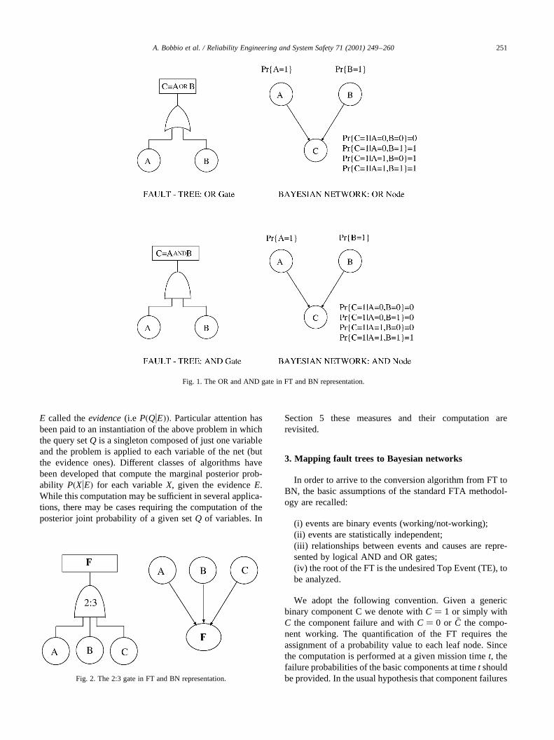
Fig. 1. The OR and AND gate in FT and BN representation.

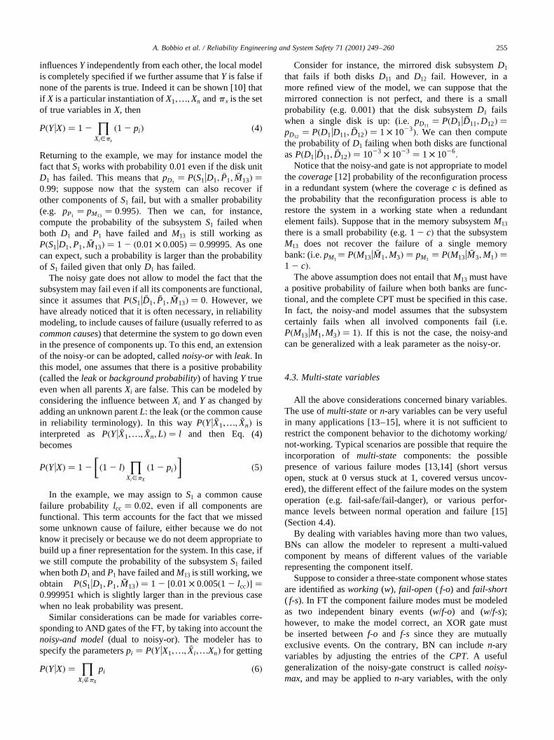
Fig. 2. The 2:3 gate in FT and BN representation.

are exponentially distributed, the probability of occurrenceof the primary event�C � 1� faulty� is P�C � 1; t� � 1 2e2lCt

; wherelC is the failure rateof componentC.We first show how an FT can be converted into an equiva-

lent BN and then we show, in Section 4, how assumptions(i)–(iii) can be relaxed in the new formalism. To proceedstep by step, Fig. 1 shows the conversion of an OR and anAND gate into equivalent nodes in a BN. Parent nodesA andB are assigned prior probabilities (coincident with the prob-ability values assigned to the corresponding basic nodes inthe FT), and child nodeC is assigned its CPT. Since, the ORand AND gates represent deterministic causal relationships,all the entries of the corresponding CPT are either 0s or 1s.

A common extension to many FT packages is to haveimplicit �k : n� gates. Implicit gate means, that the FT solvermust explicit the Boolean expression of the�k : n� function.The BN representation of a (2:3) is given in Fig. 2. The CPTassigned to nodeF has the following entries (these are alsoeither 0s or 1s):

Pr{F � 1uA� 0;B� 0;C � 0} � 0

Pr{F � 1uA� 0;B� 0;C � 1} � 0

Pr{F � 1uA� 0;B� 1;C � 0} � 0

Pr{F � 1uA� 1;B� 0;C � 0} � 0

Pr{F � 1uA� 0;B� 1;C � 1} � 1

Pr{F � 1uA� 1;B� 0;C � 1} � 1

Pr{F � 1uA� 1;B� 1;C � 0} � 1

Pr{F � 1jA� 1;B� 1;C � 1} � 1

�2�

It is clear that, any Boolean function from the nodesA, BandC to the nodeF can be made explicit in the BN repre-

sentation of Fig. 2 by only modifying the correspondingCPT.

According to the translation rules for the basic gates, it isstraightforward to map an FT into a binary BN, i.e. a BNwith every variableV having two admissible values:false� �V� corresponding to anormalor workingvalue andtrue (V)corresponding to afaulty or not-workingvalue. The conver-sion algorithm proceeds along the following steps:

• for eachleaf node(i.e. primary event or system compo-nent) of the FT, create aroot nodein the BN; however, ifmore leaves of the FT represent the same primary event(i.e. the same component), create just one root node in theBN;

• assign to root nodes in the BN the prior probability of thecorresponding leaf node in the FT (computed at a givenmission timet);

• for eachgateof the FT, create a correspondingnodeinthe BN;

• label the node corresponding to the gate whose output isthe TE of the FT as theFault node in the BN;

• connect nodes in the BN as corresponding gates areconnected in the FT;

• for each gate (OR, AND ork:n) in the FT assign theequivalent CPT to the corresponding node in the BN(see Figs. 1 and 2).

Due to the very special nature of the gates appearing in aFT, non-root nodes of the BN are actually deterministicnodes and not random variables and the correspondingCPT can be assigned automatically. The prior probabilitieson the root nodes are coincident with the correspondingprobabilities assigned to the leaf nodes in the FT.

The mapping algorithm is illustrated through the follow-ing example concerning the redundant multiprocessorsystem shown in Fig. 3 and taken from Ref. [9]. The system


Fig. 3. A redundant multiprocessor system.

is composed of a busN connecting two processorsP1 andP2

having access to a local memory bank each (M1 and M2)and, through the bus to a shared memory bankM3, sothat if the local memory bank fails, the processor canuse the shared one. Each processor is connected to amirrored disk unit. If one of the disks fails, the proces-sor switches on the mirror. The whole system is func-tional if the bus N is functional and one of theprocessing subsystems is functional. Fig. 3 also showsthe partitioning into logical subsystems, i.e. the proces-sing subsystemsSi �i � 1;2�; the mirrored disk unitsDi

�i � 1;2� and the memory subsystemsMi3 �i � 1; 2�: TheFT for this system is shown in Fig. 4a. The logicalexpression of the TE as a function of theminimal cutsets is given by the following expression:

TE� N 1 D11D12D21D22 1 D11D12M2M3 1 D11D12P2

1 M1M3D21D22 1 M1M2M3 1 M1M3P2 1 P1D12D22

1 P1M2M3 1 P1P2 (3)


Fig. 4. (a) Fault tree and (b) Bayesian network for the multiprocessor system.

For ease of comparison, and for evidencing the connec-tion between leaf nodes in the FT and root nodes in the BN,the structure of the corresponding BN is represented in thesame Fig. 4b. As an example, in Fig. 4b, the CPT entries forthe nodeFault (corresponding to an OR gate) and for thenodeS12 (corresponding to an AND gate) are also shown. Inorder to quantify both models, the failure probabilities ofeach component are then assigned to the leaf nodes of theFT, and to the root nodes of the BN as prior probability (seeSection 5.1).

4. Modeling issues

The mapping procedure described in Section 3 shows thateach FT can be naturally converted into a BN. However,BNs are a more general formalism than FTs; for this reason,there are several modeling aspects underlying BNs that maymake them very appealing for dependability analysis. In thefollowing sections, we examine a number of extensions ofthe standard FT methodology, and we show how they can becast into a BN framework.

4.1. Probabilistic gates: common cause failures

Differently from FT, the dependence relations amongvariables in a BN are not restricted to be deterministic.This corresponds to being able to model uncertainty in thebehavior of thegates, by suitably specifying the conditionalprobabilities in theCPT entries. Probabilistic gates mayreflect an imperfect knowledge of the system behavior, ormay avoid the construction of a more detailed and refinedmodel. A typical example is the incorporation of CommonCause Failures (CCF). Common cause failures are usuallymodeled in FT by adding an OR gate, directly connected tothe TE, in which one input is the system failure, the otherinput the CCF leaf to which the probability of failure due tocommon causes is assigned. In the BN formalism, suchadditional constructs are not necessary, since the probabil-istic dependence is included in the CPT. Fig. 5 shows anAND gate with CCF and the corresponding BN. The value

LCCF is the probability of failure of the system due tocommon causes, when one or both components are up.

4.2. Noisy gates

Of particular attention for reliability aspects is one pecu-liar modeling feature often used in building BN models:noisy gates. As mentioned in Section 2, when specifyingCPT entries one has to condition the value of a variableon every possible instantiation of its parent variables,making the number of required entries exponential withrespect to the number of parents. By assuming that thenode variable is influenced by any single parent indepen-dently of the other ones (disjunctive interaction[10]), noisygates reduce this effort by requiring a number of parameterslinear in the number of parents.

Consider for example the subsystemS1 in Fig. 3: it fails ifeither the disk unitD1 or the processorP1 or the memorysubsystemM13 fails. Since nodeS1 in the BN of Fig. 4 hasthree parent nodes, this implies that the modeler has toprovide eight CPT entries for completely specify this localmodel.1 Of course if this local model is a deterministiclogical OR (as in the example), only three probabilities(equal to 1) are sufficient. Consider now the case wherethe logical OR interaction isnoisyor probabilistic: even ifone of the components ofS1 fails, there is a (possibly small)positive probability that the subsystem works. This corre-spond to the fact that the system may maintain some func-tionality or may be able to reconfigure (with someprobability of reconfiguration success) in the presence ofparticular faults.

BN can still avoid the complete CPT specification byadopting the so-callednoisy-or model. Given a binary vari-ableY having the set of parent binary variablesX1;…;Xn;

the noisy-or model requires to specifyn parametersp1;…; pn; where eachpi is interpreted as the probability ofY true given thatXi is true and all the other parents are false(i.e. pi � P�Yu �X1;…Xi ;…; �Xn��: By assuming that eachXi


Fig. 5. The CCF representation in BN.

1 The whole local model is composed of 16 entries, but only 8 have to beprovided independently becauseP�YuX� � 1 2 P� �XuY�:

influencesY independently from each other, the local modelis completely specified if we further assume thatY is false ifnone of the parents is true. Indeed it can be shown [10] thatif X is a particular instantiation ofX1;…;Xn andp x is the setof true variables inX, then

P�YuX� � 1 2Y

Xi[px

�1 2 pi� �4�

Returning to the example, we may for instance model thefact thatS1 works with probability 0.01 even if the disk unitD1 has failed. This means thatpD1

� P�S1uD1; �P1; �M13� �0:99; suppose now that the system can also recover ifother components ofS1 fail, but with a smaller probability(e.g. pP1

� pM13� 0:995�: Then we can, for instance,

compute the probability of the subsystemS1 failed whenboth D1 and P1 have failed andM13 is still working asP�S1uD1;P1; �M13� � 1 2 �0:01× 0:005� � 0:99995: As onecan expect, such a probability is larger than the probabilityof S1 failed given that onlyD1 has failed.

The noisy gate does not allow to model the fact that thesubsystem may fail even if all its components are functional,since it assumes thatP�S1u �D1; �P1; �M13� � 0: However, wehave already noticed that it is often necessary, in reliabilitymodeling, to include causes of failure (usually referred to ascommon causes) that determine the system to go down evenin the presence of components up. To this end, an extensionof the noisy-or can be adopted, callednoisy-orwith leak. Inthis model, one assumes that there is a positive probability(called theleakor background probability) of havingY trueeven when all parentsXi are false. This can be modeled byconsidering the influence betweenXi andY as changed byadding an unknown parentL: the leak (or the common causein reliability terminology). In this wayP�Yu �X1;…; �Xn� isinterpreted asP�Yu �X1;…; �Xn;L� � l and then Eq. (4)becomes

P�YuX� � 1 2

��1 2 l�

YXi [pX

�1 2 pi��

�5�

In the example, we may assign toS1 a common causefailure probability lcc � 0:02; even if all components arefunctional. This term accounts for the fact that we missedsome unknown cause of failure, either because we do notknow it precisely or because we do not deem appropriate tobuild up a finer representation for the system. In this case, ifwe still compute the probability of the subsystemS1 failedwhen bothD1 andP1 have failed andM13 is still working, weobtain P�S1uD1;P1; �M13� � 1 2 �0:01× 0:005�1 2 lcc�� 0:999951 which is slightly larger than in the previous casewhen no leak probability was present.

Similar considerations can be made for variables corre-sponding to AND gates of the FT, by taking into account thenoisy-and model(dual to noisy-or). The modeler has tospecify the parameterspi � P�YuX1;…; �Xi ;…Xn� for getting

P�YuX� �Y

XiÓpX

pi �6�

Consider for instance, the mirrored disk subsystemD1

that fails if both disksD11 and D12 fail. However, in amore refined view of the model, we can suppose that themirrored connection is not perfect, and there is a smallprobability (e.g. 0.001) that the disk subsystemD1 failswhen a single disk is up: (i.e.pD11

� P�D1u �D11;D12� �pD12� P�D1uD11; �D12� � 1 × 1023�: We can then compute

the probability ofD1 failing when both disks are functionalasP�D1u �D11; �D12� � 1023 × 1023 � 1 × 1026

:

Notice that the noisy-and gate is not appropriate to modelthecoverage[12] probability of the reconfiguration processin a redundant system (where the coveragec is defined asthe probability that the reconfiguration process is able torestore the system in a working state when a redundantelement fails). Suppose that in the memory subsystemM13

there is a small probability (e.g. 12 c� that the subsystemM13 does not recover the failure of a single memorybank: (i.e.pM1

� P�M13u �M1;M3� � pM3� P�M13u �M3;M1� �

1 2 c�:The above assumption does not entail thatM13 must have

a positive probability of failure when both banks are func-tional, and the complete CPT must be specified in this case.In fact, the noisy-and model assumes that the subsystemcertainly fails when all involved components fail (i.e.P�M13uM1;M3� � 1�: If this is not the case, the noisy-andcan be generalized with a leak parameter as the noisy-or.

4.3. Multi-state variables

All the above considerations concerned binary variables.The use ofmulti-stateor n-ary variables can be very usefulin many applications [13–15], where it is not sufficient torestrict the component behavior to the dichotomy working/not-working. Typical scenarios are possible that require theincorporation of multi-state components: the possiblepresence of various failure modes [13,14] (short versusopen, stuck at 0 versus stuck at 1, covered versus uncov-ered), the different effect of the failure modes on the systemoperation (e.g. fail-safe/fail-danger), or various perfor-mance levels between normal operation and failure [15](Section 4.4).

By dealing with variables having more than two values,BNs can allow the modeler to represent a multi-valuedcomponent by means of different values of the variablerepresenting the component itself.

Suppose to consider a three-state component whose statesare identified asworking (w), fail-open ( f-o) and fail-short( f-s). In FT the component failure modes must be modeledas two independent binary events (w/f-o) and (w/f-s);however, to make the model correct, an XOR gate mustbe inserted betweenf-o and f-s since they are mutuallyexclusive events. On the contrary, BN can includen-aryvariables by adjusting the entries of theCPT. A usefulgeneralization of the noisy-gate construct is callednoisy-max, and may be applied ton-ary variables, with the only


constraint of having an order defined on the set of the admis-sible values of the variables [16].

4.4. Sequentially dependent failures

Another modeling issue that may be quite problematic todeal with using FT is the problem of components failing insome dependent way. For instance, the abnormal operationof a component may induce dependent failures on otherones. Suppose for instance that we refine the descriptionof the multiprocessor system by adding the componentpower supply (PS) such that, when failing, causes a systemfailure, but it may also induce the processors to break down.In the FT representation, a new input PS should be added tothe TE of Fig. 4 to represent a new cause of system failure asshown in Fig. 6a; however, modeling the dependencebetween the failure of PS and the failure of processorPi �i �1; 2� is not possible in the FT formalism.

Notice that, in the BN model one may be even moreprecise, by resorting to a multi-state model for the powersupply; indeed, a more realistic situation could be thefollowing: PS is modeled with three possible modes:correct, defectiveand deadwhere the first corresponds toa nominal behavior, the second to a defective working modewhere an abnormal voltage is provided, while the last corre-sponds to a situation where PS cannot work at all. Of course,deadmode causes the whole system to be down, but wewant to model the fact that when PS is in thedefectivemode the processors increase their conditional dependenceto break down. This can be modeled in a very natural way,by considering the variable PS to have three values corre-sponding to the above modes and by setting the entries in theCPT in a suitable way.

5. Analysis issues

Typical analyses performed on a FT involve both quali-tative and quantitative aspects. In particular, any kind ofquantitative analysis exploits the basics of the qualitativeanalysis, thus the minimal cut-sets computation. Minimalcut-sets are the prime implicants of the TE and are usuallyobtained by means of minimization techniques on the set oflogical functions represented by the Boolean gates of theFT. Given the set of minimal cut-sets, usual quantitativeanalysis involves:

• the computation of the overall unreliability of the systemcorresponding to the unreliability of the TE (i.e.P(Fault));

• the computation of the unreliability of each identifiedsubsystem, corresponding to the unreliability of eachsingle gate;

• the importance of each minimal cut-set, corresponding tothe probability of the cut-set itself by assuming the statis-tical independence among components.

In particular, if each componentci has probability of fail-ure P�ci�; the importance of a cut-set CS is given byP�CS� � Q

ci [CSP�ci�: Notice that such a quantity refersto the a-priori failure probability of each component.

As shown in Section 3, any FT can be mapped into a BNwhere non-root nodes are deterministic. Any analysisperformed on a FT can be performed on the correspondingBN; moreover, other interesting measures can be obtainedfrom the BN, that cannot be evaluated in an FT. Let us firstconsider the basic analyses of a FT and how they areperformed in the corresponding BN:

• unreliability of the TE:this corresponds to computing theprior probability of the variableFault, that isP�QuE� withQ� Fault andE � 0;

• unreliability of a given subsystem:this corresponds tocomputing the prior probability of the correspondingvariableSi, that isP�QuE� with Q� Si andE � 0:

Differently from the computations performed on an FT,the above computations in a BN do not require the determi-nation of the cut-sets. However, any technique used for cut-set determination in the FT can be applied in the BN:indeed, the Boolean functions modeled by the gates in theFT are modeled by non-root nodes in the BN.

Concerning the computation of the cut-set importance, itis worth noting that BN may directly produce a more accu-rate measure of such an importance, being able to providethe posterior probability of each cut-set given the fault.Indeed, posing a query having the nodeFault as evidenceand the root variablesR as queried variables allows one tocompute the distributionP�RuFault�; this means that theposterior probability of each mode of each component(just workingandfaulty in the binary case) can be obtained.Once cut-sets are known, the computation of the posteriorimportance is just a matter of marginalization onP�RuFault�:

Related to the above issue is another aspect that is pecu-liar of the use of BN with respect to FT: the possibility ofperforming diagnostic problem-solvingon the modeledsystem. In fact, in many cases the system analyst may beinterested in determining the possible explanations of anexhibited fault in the system. Cut-set determination is astep in this direction, but it may not be sufficient in certainsituations. Classical diagnostic inference on a BN involves:

• computation of the posterior marginal probability distri-bution on each component;

• computation of the posterior joint probability distributionon subsets of components;

• computation of the posterior joint probability distributionon the set of all nodes, but the evidence ones.

The first kind of computation is perhaps the most popularone when using BN for diagnosis (see for instance DXpress[16] or MSBN [17] or HUGIN [18] tools). One advantage is


that there exist well-established algorithms that cancompute the marginal posterior probability of eachnode by considering this task as if it was a singlequery (i.e. it is not necessary to pose more queries ofthe type P�QuE�; each time consideringQ equal to thenode for which we want the posterior distribution).Moreover, this kind of computation is very useful fordetermining the criticality of the components of the

system, in case a fault is observed [4]. The main disad-vantage is that considering only the marginal posteriorprobability of components is not always appropriate fora precise diagnosis [10]; in many cases the right wayfor characterizing diagnoses is to consider scenariosinvolving more variables (for example all the compo-nents). The other two kinds of computation addressexactly this point.


Fig. 6. Adding power supply: (a) fault tree; (b) Bayesian network.

5.1. Example

Consider the multiprocessor system of Fig. 3. The failuredistribution of all components is assumed to be exponentialwith the failure rates (expressed inf/h units) given in Table1. The dependability measures are required to be evaluatedat a mission timet � 5000 h: The failure probabilities ofeach component, evaluated att � 5000 h is reported in thesecond column of Table 1 (prior failure probabilities).

Forward propagation on the BN allows us to compute theunreliability of the TE as the a priori probability of systemfailure, i.e.P�Fault� � 0:012313:

If we observe that the system is faulty at timet, themarginal posterior fault probabilities of each componentare then computed, and are reported on the third columnof Table 1. This measures may be useful to provide anindication of the criticality of each single component ifthe system is faulty; observe that the severity rankingbased on posteriors is different from the one based on priors.We can also notice that the most critical component is in thiscase each disk. However, this information is not completelysignificant from the diagnostic point of view; indeed, byconsidering the disk units, the only way of having thefault is to assume that all the disksD11, D12, D21, D22 havefailed at the same time (indeed, it is the only minimal cut-setinvolving only disks). This information (the fact that alldisks have to be jointly considered faulty to get the fault)is not directly derived by marginal posteriors on compo-nents. In fact, for diagnostic purposes a more suitable analy-sis should consider the posterior joint probability of all thecomponents given the system fault as evidence. This analy-sis corresponds to search the most probable state given thefault, over the state space represented by all the possibleinstantiations of the root variables (i.e. components).

In this case, we can determine by means of BN inferencethat the most probable diagnosis (i.e. the most probable stategiven the system fault) is exactly the one corresponding tothe faulty value of all the disks and the normal value of allthe other components; in particular, we obtain:

P� �N; �M1; �M2; �M3; �P1; �P2;D11;D12;D21;D22uFault� � 0:95422

Notice that the above diagnosis does not correspond to thecut-set {D11;D12;D21;D22} ; since the latter does not implythat the unmentioned components are working (i.e. assignedto the normal value); anyway, the posterior probability ofthe cut-sets can be naturally computed in the BN setting by a

query on all the disk variables conditioned on the observa-tion of the fault.

In a reliability context, it seems more reasonable torestrict the attention only to root variables. However, analternative way of characterizing diagnoses is to viewthem as complete assignments to all the variables but theevidence ones; this corresponds to search over the statespace of all the possible instantiations of every variable inthe BN. When the task consists in computing the most prob-able of such diagnoses it is called MPE computation [10](where MPE stands formost probable explanation).

An interesting possibility offered by BN is that there existalgorithms able to produce diagnoses (either viewed asonly-root assignments or all-variable assignments) inorder of their probability of occurrence, without exploringthe whole state space; they are usually calledany-timealgo-rithms, since the user can stop the algorithm at any time, bygetting an approximate answer that is improved if more timeis allocated to the algorithm. For example, an algorithmbased on the model described in Ref. [19] is able to providethe most probable diagnoses, given the observation of thefault, in the multiprocessor system at any desired level ofprecision. By specifying a maximum admissible errore inthe posterior probability of the diagnoses, the algorithm isable to produce every diagnosisD, in decreasing order oftheir occurrence probability, with an estimateP0�DuFault�such that its actual posterior probability isP�DuFault� �P0�DuFault� ^ e:

In the example, by requiring diagnoses to be root assign-ments ande � 1 × 1026 the first three diagnoses are, inorder:

d1 : � �N; �M1; �M2; �M3; �P1; �P2;D11;D12;D21;D22�

d2 : � �N; �M1; �M2; �M3; �P1;P2;D11;D12; �D21; �D22�

d3 : � �N; �M1; �M2; �M3;P1; �P2; �D11; �D12;D21;D22�The first one represents the already mentioned most prob-able diagnoses with all disks faulty, while the second andthe third one are two symmetrical diagnoses:d2 represents afault caused by disk failures in the first sub-system and aprocessor failure in the second;d3 represents a fault causedby disk failures in the second sub-system and a processorfailure in the first.

Posterior probabilities are then computed within the


Table 1Component failure rate, prior and posterior probabilities

ComponentC Fail. ratelC (f/h) Prior fail. prob. Pr(C) Posterior fail. prob. Pr(CuTE)

Disk Dij lD� 8.0× 1025 0.32968 0.98436ProcPi lP� 5.0× 1027 0.00025 0.02252Mem Mj lM� 3.0× 1028 0.000015 0.000015BusN lN� 2.0× 1029 0.00001 0.000081

given error level as

P�d1uFault� � 0:954223

P�d2uFault� � P�d3uFault� � 98:87× 1024

The algorithm guarantees that any further diagnosis hasa posterior probability smaller or equal thanP�d2uFault�:It is worth noting that this result is in general obtainedwithout exploring the whole state space, that in thiscase is equal to 210 � 1024 states, 10 being the numberof components.

Similar results may be obtained for complete variableassignments. Notice that if the BN has only deterministicnon-root nodes, a root assignment uniquely corresponds to acomplete assignment with the same posterior, because givena particular assignment of modes to components, the assign-ment to non-root variables is deterministically obtained.This is no longer true if we introduce uncertainty at innerlevels as it is usually done within BN.

Concerning the complexity of probabilistic computationusing BN, the general problem of computing posterior prob-abilities on an arbitrary net is known to be NP-hard [20],however the problem reduces to a polynomial complexity ifthe structure of the net is such that the underlying undirectedgraph contains no cycles. Even if in practice this restrictionis not often satisfied, research on efficient probabilisticcomputation has produced considerable results showingthat acceptable computation can be performed even innetworks with general structure and hundreds of nodes[21–23].

6. Conclusions and current research

Bayesian networks provide a robust probabilistic methodof reasoning with uncertainty and are becoming widely usedfor dependability analysis of safety critical systems as theProgrammable Electronic Systems (PES). During PES life-cycle, dependability analysis are performed at differentlevels addressing hardware, software and the whole system.Here, we have dealt with BN versus FT, a very populartechnique for hardware dependability analysis. BN versusFT can address interesting questions allowing both forwardand backward analysis; moreover, BN are more suitable torepresent complex dependencies among components and toinclude uncertainty in modeling. Due to the presence of thesoftware component, there is a major concern on how theoverall PES dependability is evaluated. Software faults andhuman errors introduce design faults in PES. Probabilisticanalysis of software dependability is a formidable task, forwhich no proven method is available. BN seems to bepromising for sounder assessment of software dependability[24]. Overall system dependability, due the impact of designfaults, is not well understood. The evaluation of overallsystem dependability can be obtained by considering andcombining all the different sources of relevant information

(evidence), including software and hardware dependabilityanalysis [7]. The possibility of use of BN to support theevaluation of overall system dependability along the accep-tance process of safety critical PES is under exploration.Although the use of BN seems to be promising at differentlevels of PES dependability analysis, they do not provide adirect mechanism for representing temporal dependencies,that are well implemented in popular techniques for depend-ability analysis, such as Markov Chains and Stochastic PetriNets.

References

[1] Henley EJ, Kumamoto H. Reliability engineering and risk assess-ment. Englewood Cliffs, NJ: Prentice Hall, 1981.

[2] Leveson NG. Safeware: system safety and computers. Reading, MA:Addison-Wesley, 1995.

[3] Heckermann D, Wellman M, Mamdani A, editors. Real-world appli-cations of Bayesian networks. Communications of the ACM1995;38(3).

[4] Almond G. An extended example for testing Graphical Belief. Tech-nical Report 6: Statistical Sciences Inc., 1992.

[5] Portinale L, Bobbio A. Bayesian networks for dependability analysis:an application to digital control reliability. Proceedings of the 15thConference on Uncertainty in Artificial Intelligence, UAI-99, 1999. p.551–8.

[6] Bobbio A, Portinale L, Minichino M, Ciancamerla E. Comparingfault trees and Bayesian networks for dependability analysis.Proceedings of the 18th International Conference on ComputerSafety, Reliability and Security, SAFECOMP99, vol. 1698, 1999.p. 310–22.

[7] Fenton N, Littlewood B, Neil M, Strigini L, Sutcliffe A, Wright D.Assessing dependability of safety critical systems using diverseevidence. IEEE Proc Software Engng 1998;145(1):35–9.

[8] Torres-Toledano JG, Sucar LE. Bayesian networks for reliabilityanalysis of complex systems, Lecture notes in artificial intelligence,vol. 1484. Berlin: Springer, 1998 (p. 195–206).

[9] Malhotra M, Trivedi K. Dependability modeling using Petri nets.IEEE Trans Reliabil 1995;R-44:428–40.

[10] Pearl J. Probabilistic reasoning in intelligent systems. Los Altos, CA:Morgan Kaufmann, 1989.

[11] Neapolitan RE. Probabilistic reasoning in expert systems. New York:Wiley, 1990.

[12] Dugan JB, Trivedi KS. Coverage modeling for dependability analysisof fault-tolerant systems. IEEE Trans Comput 1989;38:775–87.

[13] Garribba S, Guagnini E, Mussio P. Multiple-valued logic trees:meaning and prime implicants. IEEE Trans Reliabil 1985;R-34:463–72.

[14] Doyle SA, Dugan JB, Patterson-Hine A. A combinatorial approach tomodeling imperfect coverage. IEEE Trans Reliabil 1995;44:87–94.

[15] Wood AP. Multistate block diagrams and fault trees. IEEE TransReliabil 1985;R-34:236–40.

[16] Knowledge Industries. DXpress 2.0, 1996.[17] Microsoft Corporation. Microsoft Belief Network Tools.[18] Andersen SK, Olesen KG, Jensen FV. HUGIN — a shell for building

Bayesian belief universes for expert systems. Proceedings of the 11thIJCAI, Detroit, MI, 1989. p. 1080–5.

[19] Portinale L, Torasso P. A comparative analysis of Horn models andBayesian networks for diagnosis, Proceedings of the 5th ItalianConference on Artificial Intelligence. Berlin: Springer, 1997.

[20] Cooper G. The computation complexity of probabilistic inferenceusing Bayesian belief networks. Artific. Intell 1990;33:393–405.

[21] Kjaerulff U. Aspects of efficiency improvements in Bayesian


networks. Technical Report. Thesis, Faculty of Technology andScience, Aalborg University, 1993.

[22] Poole N, Zhang L. Exploiting causal independence in Bayesiannetwork inference. J Artific Intell Res 1996;5:301–28.

[23] D’Ambrosio M, Takinawa. Multiplicative factorization of noisy-max.

Proceedings of the 15th Conference on Uncertainty in Artificial Intel-ligence UAI99, Stockholm, 1999. p. 622–30.

[24] Delic KA, Mazzanti F, Strigini L. Formalising engineering judgementon software dependability via Belief Networks. Technical Report,SHIP, 1995.


improving the analysis of dependable systems by...

Documents