Improving the asset pricing ability of theConsumption-Capital Asset Pricing Model?

Anne-Sofie Reng Rasmussen

Keywords: C-CAPM, intertemporal asset pricing, conditional assetpricing, pricing errors.Preliminary 1. draft.

Abstract

This paper compares the asset pricing ability of the traditional consumptionbased capital asset pricing model to models from two strands of literature at-tempting to improve on the poor empirical results of the C-CAPM. One strandis based on the intertemporal asset pricing model of Campbell (1993, 1996) andCampbell and Vuolteenaho (2004). The model takes the traditional C-CAPM asits starting point, but substitutes all references to consumption out, as empiricalconsumption data is assumed to be error ridden.The other strand to be investigated is based on the premise that the C-

CAPM is only able to price assets conditionally as suggested by Cochrane (1996)and Lettau and Ludvigson (2001b). The unconditional C-CAPM is rewritten asa scaled factor model using the approximate log consumption-wealth ratio cay,developed by Lettau and Ludvigson (2001a), as scaling variable.The models are estimated on US data and the resulting pricing errors are

compared using average pricing errors and a number of composite pricing errormeasures. Models from both the alternative literature strands are found tooutperforme the traditional C-CAPM. The conditional C-CAPM and the twobeta I-CAPM of Campbell and Vuolteenaho (2004) result in pricing errors ofapproximately the same size, both average and composite. Thus, there is nounambigous solution to solving the pricing ability problems of the C-CAPM.

I IntroductionThe consumption-based capital asset pricing model (C-CAPM) introduced byLucas (1978), Breeden (1979), and Grossman and Shiller (1981), determinesasset risk by the covariance of the asset’s return with marginal utility of con-sumption. However, empirical investigations have lent little support to therelations obtained from the model. Tests of the C-CAPM have led to rejec-tion of the model as well as unrealistic parameter estimates resulting in theestablishment of the so-called "equity premium puzzle" (Hansen and Singleton(1983), Mehra and Prescott (1985), Kocherlakota (1996)). This in spite of thefact that the model is of an intertemporal nature, in the spirit of the I-CAPMof Merton (1973). In fact, the model is found to be outperformed by the sta-tic CAPM (Mankiw and Shapiro (1986)) and unrestricted multifactor models,when it comes to explaining cross sectional asset returns.Despite the empirical failures of the consumption based model, the economic

intuition underlying the model is so intuitively appealing that it would be amistake to dismiss it completely. It also has the property that models such asthe CAPM and the APT, can be mapped into the framework as special cases,as pointed out by Cochrane (2001). The relation linking the marginal utility ofconsumption to asset returns still holds, but additional assumptions are madeenabling other variables to be used in place of consumption. So if the modelcan’t be dismissed, why is it failing empirically?This paper looks at two strands of literature addressing the poor empirical

findings of the C-CAPM. One is the I-CAPM of Campbell (1993, 1996) andCampbell and Vuolteenaho (2004). This is an intertemporal model, based onthe same framework as the C-CAPM, but rephrased without reference to con-sumption data. The other strand looks at the conditional pricing ability of theC-CAPM in a scaled factor setup, as in Cochrane (1996), Ferson and Harvey(1999), and Lettau and Ludvigson (2001b).These models take two different directions, but with the common goal of

improving on the empirical performance of the C-CAPM. The question is, dothey succeed? This paper will compare the asset pricing ability of the traditionalC-CAPM with that of these alternative models.The first strand to be investigated is based on the argument of Campbell

(1993), that the poor empirical performance of the C-CAPM may be due toproblems inherent in the empirical consumption data used to test the model,rather than with the theoretical assumptions underlying. Firstly, aggregateconsumption data are measured with error and are time-aggregated (Grossman(1987), Wheatley (1988), and Breeden et al. (1989)). Secondly, the consumptionof asset-market participants may be poorly proxied by aggregate consumption(Mankiw and Zeldes (1991)).To address these issues Campbell (1993) develops an intertemporal model,

which uses the same building blocks as the C-CAPM, but makes no referencesto consumption data. Using a first order Taylor expansion of the intertempo-ral budget constraint of the representative investor and combining it with alog-linear Euler equation, one is able to express unanticipated consumption as

1

a function of expectational revisions in current and future returns to wealth,thereby eliminating all references to consumption. The model can thus be esti-mated empirically without running into consumption data issues usually facedwhen testing the C-CAPM. In Campbell and Vuolteenaho (2004), the model isrewritten in a two-beta notation and is found to give an explanation for the sizeand value anomalies found when estimating traditional asset pricing models suchas the CAPM and C-CAPM. Campbell and Vuolteenaho (2004) compare thepricing errors of their model to the CAPM, but do not estimate the C-CAPM.The other strand of literature treated in this paper looks at the conditional

pricing ability of the C-CAPM in a scaled factor setup. That is, it is assumedthat the cause of the poor empirical performance of the C-CAPM is that themodel is in fact only able to price assets conditionally. This would allow forrecent empirical evidence of time variation in expected returns. By estimatingthe models conditionally, we can incorporate time-varying risk premia into themodels. Lettau and Ludvigson (2001b) find that the conditional version of theC-CAPM, using the approximate log consumption-wealth ratio cay as scalingvariable, is also able to explain the value and size anomalies. The model per-forms far better than the unconditional C-CAPM and about as well as the threefactor model of Fama and French (1993).Both strands of literature have had some success in explaining the empir-

ical anomalies the C-CAPM fails to fit. But how do the models compare toeach other? Is one of the model strands unequivocally better than the other atfitting the historical data? Do we have a clear cut empirical replacement forthe C-CAPM? To answer these questions we first look at the statistical signif-icance of the pricing errors resulting from the various models. In order to lookinto the relative pricing ability, both the average squared pricing errors and acomposite pricing error, created by weighting pricing errors by the variance ofthe respective asset returns, are investigated. These measures will give us anidea of the economic magnitude of the pricing errors of the models. Finally, thedistance measure of Hansen and Jagannathan (1997) is also computed. Thiscan be interpreted as the maximum pricing error pr. unit payoff norm.Estimation of the traditional asset pricing models undertaken in this paper

support the findings of previous research. The CAPM and C-CAPM result ininsignificant coefficient estimates and high pricing errors. When looking at thecross sectional estimates the Fama-French model are somewhat unstable. Theestimated risk price on the market return becomes negative. This is unlike pre-vious findings in the literature, as reported by Lettau and Ludvigson(2001b).If the sample period is restricted from our sample to the slightly shorter subpe-riod used in Lettau and Ludvigson, positive coefficient estimates are once againobtained. Thus, the risk price on the market return of the Fama-French modelappears very unstable in cross sectional estimations. This is due to the relativelylow degree of variation in market return betas across average portfolio returns.In fact, eliminating the market return risk factor from the Fama-French modelmakes almost no difference to the cross-sectional pricing ability of the model.The conditional versions of the CAPM and C-CAPM do a better job of

fitting the data than the traditional unconditional models, although especially

2

the conditional C-CAPM still has problems with insignificant coefficients. Theintertemporal model of Campbell and Vuolteenaho (2004) also outperforms thetraditional models. Pricing errors are reduced and the unconditional equitypremium is fitted relatively well. However, when comparing the pricing abilityof the two alternative strands, we cannot point to one setup as the obviousreplacement for the traditional C-CAPM. There is no distinct difference in thepricing ability of the two strands, when comparing the various weighted pricingerror measures.The paper is structured in the following manner. Section II will present the

different asset pricing models to be considered. Section III describes the empir-ical estimation techniques used. The data is described in section IV, empiricalresults in section V and finally in section VI we conclude.

II The ModelsIn the absence of arbitrage, a stochastic discount factor Mt+1 exists, such thatany asset return Ri,t+1 obeys the following relation

1 = Et [Mt+1Ri,t+1] (1)

Ri,t+1 is the gross return on asset i from time t to t+ 1, Mt+1 is the stochasticdiscount factor or pricing kernel, and Et is the conditional expectation operator.The question we face is, how is the stochastic discount factor to be expressed?The economic argument of the consumption based asset pricing model (C-

CAPM) is that Mt+1 should be a measure of the marginal rate of substitution.In order for an agent to invest in a given asset at time t, the expected return attime t+ 1 must compensate for the consumption possibilities given up at timet. In the C-CAPM, the stochastic discount factor is thus given by

Mt+1 = δu0 (ct+1)

u0 (ct). (2)

δ is the subjective rate of time preference discount factor, u (•) is the utilityfunction, and ct denotes consumption. Despite the strong underlying economicintuition, the empirical performance of this model has been poor. If we don’twish to disregard the model completely, we have to look at what factors may becausing the empirical problems. Are there some deviations between the simpleeconomic theory presented in (1) and (2) and the empirical estimates. If we lookat where problems could arise, three places spring to mind. Firstly, to estimatethe C-CAPM we must choose an operational form of the utility function. Manyutility functions have been suggested, but the traditional C-CAPM is based onthe power utility function. This may however be an inaccurate description of theutility function of agents and hence the model may be failing on these grounds.Secondly, the functional forms of (2) traditionally associated with the C-CAPMassume constant risk premia. Evidence of time-variation in expected returns,on the contrary, make it desirable to allow for time-variation in the risk premia

3

of the model. The problem with the C-CAPM may thus be, that in actualityit only holds conditionally. Finally, estimation of the C-CAPM requires the useof an empirical measure of the consumption of the marginal investor ct. This ismost often proxied by some measure of aggregate consumption in the economy,often based on expenditures on goods and services. Any deviations between thetheoretical consumption measure and the empirical data may be resulting in thepoor empirical performance of the C-CAPM.Attempts have been made to rectify the empirical struggles of the C-CAPM,

by developing factor models with SDF’s that form good proxies for the righthand side of (2), and take the three problems described above into consideration.In this paper we will look at whether these attempts help or harm the pricingability of the C-CAPM.The models treated in the following can all be mapped into the linear factor

model framework. In this case, Mt+1 is quantified as a linear combination of anumber of factors determined by the underlying theory of the given model. LetF0t+1 =

£1, f 0t+1

¤, where f 0t+1 is the vector of factors included in the model. The

stochastic discount factor is given by

Mt+1 = cFt+1 (3)

where c = [1,b0] and b is the vector of coefficients on the variable factorsof the model. As noted by Cochrane (2001), all factor models are in realityspecializations of the consumption-based model. Some additional assumptionsare made, allowing marginal utility growth to be replaced by other economicallyrelevant factors, such that the right hand side of (2) is proxied by the right handside of (3).In order to estimate the factor models cross-sectionally, we rewrite them in

a beta representation. Inserting (3) into the general pricing equation (1), takingunconditional expectations and applying a variance decomposition results in thefollowing cross-sectional multifactor model

E [Ri,t+1 −Rf,t+1] = β0iλ (4)

βi ≡ cov (f , f 0)−1

cov (f , Ri,t+1) (5)

λ ≡ −E [Rf,t+1] cov (f , f0)b (6)

Rf,t+1 is the risk-free rate of return, for which it holds that Rf,t+1 =1

E(Mt+1).

We have introduced the general linear factor model framework and nowcomes the time to look at which factors are included in the specific modelsstudied in this paper.

II.1 Traditional asset pricing models

As noted in the previous section, the stochastic discount factor of the C-CAPMis based on the marginal rate of substitution of consumption. To estimate themodel, one in principal needs to decide how to model the utility function. Often

4

power utility is applied. However extensions using the more general Epstein-Zin-Weil utility and habit based functions have also been introduced. To avoidbeing constrained by the choice of utility function, it is assumed that M can beproxied by a linear function of log consumption growth ct+1

Mt+1 ≈ a+ b∆ct+1 (7)

This approximation holds, regardless of the functional form of the investorsutility. As is evident, (7) is a linear factor model with log consumption growth asthe sole factor. It is also referred to as the log-linearized C-CAPM. Traditionally,the parameters a and b are taken to be time invariant, which will also be thecase for the base model of this paper. From (4) we find the cross-sectional assetpricing model, in beta representation

E [Ri,t+1 −Rf,t+1] = βi,∆cλ∆c (8)

This is the model that forms the basis of our investigation. A simple equationwhich relates asset returns to consumption growth.Although the focus of this paper is on the C-CAPM, and attempts to improve

on its poor empirical performance, we also include two other well known assetpricing models. This allows us to get a sense of the level of pricing errors weare experiencing in the consumption based setup, compared to other modelstraditionally estimated in the literature. The two models are the CAPM andthe three factor Fama-French (1993) model.The SDF of the CAPM with time invariant parameters can be written as

Mt+1 ≈ a+ bRm,t+1 (9)

where Rm,t+1 is the return on the aggregate market. In beta representation wehave

E [Ri,t+1 −Rf,t+1] = λRmβi,Rm (10)

As Cochrane (2001) points out, the CAPM is in fact contained in the C-CAPMas a special case, adding additional motivation for the introduction of theCAPM.The Fama-French model is slightly different from the other models investi-

gated, in that it is empirically, not theoretically, driven. The factors are chosenbased on patterns observed in data, rather than being derived from an under-lying economic theory. The three factors of the model are the return on theaggregate market Rm,t+1, known from the CAPM, the return on the "smallminus big" portfolio (SMB), and the return on the "high minus low" portfolio.

Mt+1 ≈ a+ b1Rm,t+1 + b2SMBt+1 + b3HMLt+1 (11)

SMB and HML are constructed in Fama and French (1993), and are based on 6portfolios sorted on size and the ratio of book equity to market equity (BE/ME)of the assets. SMB is the difference in returns between the small and big stock

5

portfolios, sorted by size. HML is the difference in returns on the high- andlow-BE/ME portfolios.Finally, we estimate a two factor model which combines the factors of the

C-CAPM and the CAPM

Mt+1 ≈ a+ b1Rm,t+1 + b2∆ct+1 (12)

The motivation for this model, should become evident when the I-CAPM ofCampbell and Vuolteenaho (2004) is introduced. In order to develop that model,Campbell (1993) bases his derivations on a C-CAPM with Epstein-Zin-Weil(EZW) utility. A log-linearization of the EZW C-CAPM results in a two factormodel of the form presented in (12). Hence, when we compare the I-CAPM tothe original consumption based asset pricing framework, it makes sense to usethe functional form on which the I-CAPM is based.

II.2 Conditional models

The models presented so far, have all been assumed to price assets uncondition-ally. However, the cause of the empirical failure of the C-CAPM may be thatthe model is in fact only able to price assets conditionally. In recent years therehas been increasing evidence indicating predictability in excess stock returns.Predictability implies that expected returns can vary over time. This variationin investors expectations of asset returns may be due to time varying risk pre-mia. The risk premia can become state dependent if agents require a higher riskpremium to invest in stocks in times of recession for example as proposed byCampbell and Cochrane (1999). The traditional C-CAPM and CAPM do notallow for such time variation in risk premia and Lettau and Ludvigson (2001b)suggest this to be a reason for the empirical failure of the models.To model time-variation in risk premia, we need to let the weights on the

factors in the pricing kernel become time dependent

Mt+1 = at + btft+1. (13)

In order to estimate this model, Cochrane (1996) and Ferson and Harvey (1999)show that we can scale the factors in the SDF with instruments containing timet information, allowing us once more to estimate the model unconditionally.First, model the parameters as linear functions of the instrument zt

at = γ0 + γ1zt

bt = η0 + η1zt

The pricing kernel with time varying coefficients can then be rewritten as

6

Mt+1 = at + btft+1

= (γ0 + γ1zt) + (η0 + η1zt) ft+1

= γ0 + γ1zt + η0ft+1 + η1 (ztft+1) (14)

and we are back in the unconditional framework with time invariant coefficients.For the consumption based model this results in

Mt+1 = at + bt∆ct+1 = γ0 + γ1zt + η0∆ct+1 + η1 (zt∆ct+1) (15)

Equivalently, if we substitute Rm,t+1 into the above equation instead of ∆ct+1we obtain the conditional CAPM.In matrix notation

Mt+1 = c0Ft+1 (16)

with Ft+1 =£1, zt, f

0t+1, f

0t+1zt

¤0=h1, f

0t+1

i, f t+1 =

£zt, f

0t+1, f

0t+1zt

¤0, where ft+1

is a k×1 vector of k factors, c = [γ0,b0]0 where γ0 is a scalar and b = [γ1,η

00,η

01].

Inserting this into the general pricing equation (1), taking unconditionalexpectations and applying a variance decomposition results in the followingcross sectional multifactor model in beta representation

E [Ri,t+1 −Rf,t+1] = β0iλ (17)

βi ≡ cov³f , f

0´−1cov

¡f , Ri,t+1

¢λ ≡ −E [Rf,t+1] cov

³f , f

0´b

where β is the vector of regression coefficients stemming from regressing returnsRi,t+1 on Ft+1, λ is a free parameter vector and Rf,t+1 is the return on the zero-beta portfolio or risk-free rate of return.In order to estimate conditional factor models, we need to choose a vector

zt of scaling variables. The conditional models state that the coefficients on thefactors in the SDF of the factor model are dependent on the investors informa-tion set at time t. Hence the scaling variables need to describe the state of thebusiness cycle at time t. As it would be impossible to include all information inthe investors information set in an empirical estimation, we need to find vari-ables that summarize all relevant effects. On the other hand, we need to takeinto account the tractability of empirical estimation when choosing the scalingvariables. To avoid an explosion in the number of parameters to be estimated,relative to the length of the time-series of data used in this paper, we limit thenumber of scaling variables to one.Lettau and Ludvigson (2001b) suggest using the variable cay as the scaling

variable in the conditional factor models. cay can be described as a proxy

7

for the log consumption-aggregate wealth ratio and it may be used to forecastexcess stock market returns. It is calculated as cayt = ct − ωat − (1− ω) yt,where ct is consumption, at is asset wealth, and yt is labour income. ω is theaverage share of asset wealth in total wealth. The three variables are assumedto be cointegrated and ω is computed as a cointegrating coefficient. Lettauand Ludvigson (2001a, 2005) show that cayt is able to forecast excess stockreturns, better than traditional forecasting variables such as p/d and p/e ratiosat short to intermediate horizons. Hence it makes a good choice as conditioninginstrument. Hodrick and Zhang (2001) also use this variable to test conditionalfactor pricing models.

II.3 The Campbell I-CAPM

Merton (1973) builds an intertemporal capital asset pricing model where assetrisk is measured as the covariance between the asset’s return and the marginalutility of investors. By deriving the model in an intertemporal setting, innova-tions in the marginal utility of investors are driven by shocks to wealth itself, butalso by changes in the expected future returns to wealth. The ICAPM can thusbe viewed as a multi-beta version of the CAPM, but it requires all state variablesneeded to describe the characteristics of the investment opportunity set to beidentifiable. Taking this into account, empirical testing of the ICAPM quicklybecomes difficult, due to the multitude of state variables needed. This problemwas solved by the consumption-based capital asset pricing model (C-CAPM),which collapses Merton’s multi-beta pricing equation into a single-beta pricingequation. The poor empirical performance of the C-CAPM suggests, that thismay not necessarily be the right approach. One of the major problems in esti-mating the C-CAPM is the quality of the empirical consumption data neededto estimate the model. If there is a large divide between the theoretical measureof consumption growth of the model and the empirical data, then it is naturalto expect poor empirical results for the model. Not because the model as suchis faulty, but merely due to data issues.Campbell (1993) suggests a way out of this problem, by substituting con-

sumption out of the C-CAPM, but still keeping the model tractable for empiricalestimation. Under the assumption of homoskedasticity and joint lognormalityof asset returns and consumption, Campbell shows that

covt [ri,t+1,∆ct+1] = covt [ri,t+1, rm,t+1 −Etrm,t+1]

+ (1− ψ) covt

⎡⎣ri,t+1, (Et+1 −Et)∞Xj=1

ρjrm,t+1+j

⎤⎦where ri,t+1 is the log return on asset i, rm,t+1 is the log market return, ψ isthe elasticity of intertemporal substitution. Thereby, one is able to transforma log linearized C-CAPM into a cross-sectional asset pricing model, making noreferences to consumption:

8

Etri,t+1 − rf,t+1 +Vii2

= θVicψ+ (1− θ)Vim (18)

= γVim + (γ − 1)Vih (19)

Vii ≡ vart [ri,t+1]

Vic ≡ covt [ri,t+1,∆ct+1]

Vim ≡ covt [ri,t+1, rm,t+1 −Etrm,t+1]

Vih ≡ covt

⎡⎣ri,t+1, (Et+1 −Et)∞Xj=1

ρjrm,t+1+j

⎤⎦(18) states the log-linearized C-CAPM, assuming Epstein-Zin-Weil utility,

and (19) introduces the Campbell I-CAPM, in which all references to consump-tion growth have been eliminated. γ is the coefficient of relative risk aversionand θ = 1−γ

1− 1ψ

. The model states that the excess return on asset i is determined

by a weighted average of the asset return’s covariance with the current marketreturn and the return covariance with news about future market returns.Campbell and Vuolteenaho (2004) develop the model further and rewrite it

in beta representation as a two factor intertemporal model. Starting with thebasic loglinear approximate decomposition of asset returns from Campbell andShiller (1988), the following expression obtains:

ri,t+1 −Etri,t+1 = (Et+1 −Et)∞Xj=0

ρj∆di,t+1+j (20)

− (Et+1 −Et)∞Xj=1

ρjri,t+1+j

≡ Ni,CF,t+1 −Ni,DR,t+1

where ri,t+1 is the log return on asset i, di,t+1 is the log dividend on asset i, andρ is a discount coefficient1. The identity (20) states that unexpected returnsare linked to changes in expected cash flows or changes in expected discountrates. Increases in expected cash flows imply positive unexpected returns today.Increases in the expected future discount rate, on the other hand, have a negativeeffect on current returns. If future discount rates rise, we must discount cashflows by a higher rate thus resulting in a downward revision in prices today andthereby returns. This downward revision will however be reversed in the futureas increases in future discount rates also imply improved future investmentopportunities. Unlike shocks stemming from cash flow revisions, the returnshocks stemming from revisions in forecasts of discount rates are thus of a

1ρ is the average ratio of the stock price to the sum of the stock price and the dividend. ρwill be fixed at 0.95 p.a. in the empirical estimates of this paper.

9

transitory nature.Let the return rm,t+1 be given by the aggregate market return, Nm,CF,t+1 ≡

(Et+1 −Et)P∞

j=0 ρj∆dm,t+1+j, andNm,DR,t+1 ≡ (Et+1 −Et)

P∞j=1 ρ

jrm,t+1+j .The unrestricted SDF of Campbell and Vuolteenaho (2004) is

Mt+1 = a+ b1Nm,CF,t+1 + b2Nm,DR,t+1 (21)

In order to determine Nm,CF,t+1 and Nm,DR,t+1 empirically, a VAR ap-proach is used and estimated with OLS. st is a K-element state vector. Thefirst element of st is the market return. The remaining elements are variablesrelevant in forecasting future stock index returns. All variables have been de-meaned as the constants, that would otherwise arise, just capture the lineariza-tion constraints. It is assumed that st follows a first-order VAR

st+1 = Ast + ²t+1. (22)

This is not restrictive, since higher order VAR systems can be written in com-panion form. The VAR methodology enables us to express multiperiod forecastsof future returns in the following manner

Etst+1+j = Aj+1st. (23)

Define e1 as a K-element vector with first element one and the remaining el-ements zero. This vector is used to pick out the return on the market fromthe state vector st. The discounted sum of forecast revisions in returns on themarket can now be found as

Nm,DR,t+1 = (Et+1 −Et)∞Xj=1

ρjrm,t+1+j (24)

= e10∞Xj=1

ρjAj²t+1

= e10ρA (I−ρA)−1 ²t+1= e10λ²t+1,

where I is the K ×K identity matrix. Since rm,t+1 −Etrm,t+1 = e10²t+1

Nm,CF,t+1 = rm,t+1 −Etrm,t+1 +Nm,DR,t+1 (25)

= (e10 + e10λ) ²t+1

The Campbell I-CAPM can now be restated in terms of the two factorsNm,CF,t+1

and Nm,DR,t+1 derived by Campbell and Vuolteenaho (2004).

Etri,t+1−rf,t+1+Vii2= γcovt [ri,t+1,Nm,CF,t+1]−covt [ri,t+1, Nm,DR,t+1] (26)

10

Finally, we need to rephrase the model of eq.(26) in a beta representation. Definetwo beta terms based on Nm,CF,t+1 and Nm,DR,t+1

2

βi,CFm,t ≡covt (ri,t+1, Nm,CF,t+1)

vart (Nm,CF,t+1)=

σi,CFm,t

σ2CFm,t

(27)

βi,DRm,t ≡covt (ri,t+1,−Nm,DR,t+1)

vart (Nm,DR,t+1)=−σi,DRm,t

σ2DRm,t

(28)

Substitute these expressions into eq.(26) and we obtain the following cross-sectional asset pricing model

Etri,t+1 − rf,t+1 +σ2i,t2= γσ2CFm,tβi,CFm,t + σ2DRm,tβi,DRm,t (29)

By taking unconditional expectations and rewriting the left hand side of therelation in simple expected returns form, E [Ri,t+1 −Rf,t+1], we get the twobeta I-CAPM of Campbell and Vuolteenaho (2004)

E [Ri,t+1 −Rf,t+1] = γσ2CFmβi,CFm + σ2DRmβi,DRm (30)

The model will also be estimated in an unconditional, unrestricted version:

E [Ri,t+1 −Rf,t+1] = λCFβi,CFm + λDRβi,DRm (31)

We would expect the coefficient on the cash flow beta to be higher than thatfound on the discount rate beta. Since the effects of cash flow changes are ofa permanent nature, whereas those stemming from discount rate changes aretransitory, a long-term investor would be more sensitive to the shocks stemmingfrom the first beta. Hence, the investor would require a higher risk premium forholding assets with high cash-flow beta sensitivity.Finally, in the spirit of Hodrick and Zhang (2001) we also estimate a linear

SDF with a constant and those variables included in the state vector st ofCampbell and Vuolteenaho (2004) as factors. This is not an intertemporal modelas the I-CAPM, but a factor model in the spirit of the APT model. The factorsused are not innovations, but pure factors and it has none of the parameterrestrictions imposed on the Campbell and Vuolteenaho model. A comparisonwith this model will tell us, if any improvements the I-CAPM results in overthe C-CAPM are a result of the merit of the theory and techniques underlayingCampbell and Vuolteenaho (2004) or if a simple model containing the statevariables of their VAR does equally well. When comparing the models, wemust take into account the fact that the pure factor model contains more freeparameters than the Campbell and Vuolteenaho model. We should thereforenot be surprised to see some improvement in the pricing ability when using this

2The beta definition is slightly different than that rapported in Campbell & Vuolteenaho(2004). Campbell & Vuolteenaho define their betas relative to the variance on the total marketreturn instead of the variance of NCF and NDR respectively.

11

model, even if the restrictions of the I-CAPM are valid.

III Estimation techniqueTo estimate the β and λ parameters of (17) a number of econometric method-ologies could be applied. This paper uses the approach suggested by Fama andMacBeth (1973). The method is advantageous in this study due to the smallnumber of time series observations relative to the number of cross sectional port-folios treated. The dataset consists of 200 quarterly observations and 25 assetreturn portfolios. Instead of estimating the models with the Fama-MacBethmethodology, one could estimate the models by GMM. However, to get stableGMM estimates we would most likely have to reduce the number of portfoliosinvestigated. The ratio of moment restrictions to time series observations, wouldsimply be too high with all 25 portfolios. Another problem with using GMMfor this type of investigation, is the choice of weighting matrix. Fama-MacBethestimation is akin to 1. stage GMM with an identity matrix as weighting ma-trix. All 25 portfolios investigated are given equal importance when attemptingto fit the model to the data. Alternatively one could use the optimal matrix ofHansen (1982) and iterate. This would mean placing different weights on thevarious portfolios dependent on the variance of the returns. We would like themodels treated here to be able to price all 25 Fama-French portfolios equallywell, which such an approach would not take into account. One of the mainproblems with the traditional models has been their inability to price the ex-treme portfolios. Small stocks and value stocks have historically realized higherreturns than predicted by the betas of the traditional CAPM and C-CAPM.So to take an econometric approach that allows the models to place varyingweights on these portfolios, would eliminate some of the effects we are trying toinvestigate. We want to see how well the different models price these specific 25portfolios.For simplicity, the Fama-MacBeth estimation technique is described for a

one factor model. First, run time-series regressions of portfolio excess returnson the factors of the respective models to find estimates of β.

Reit = ai + β0ift + εi,t, t = 1, 2, ...., T for each i.

This gives us a beta estimate for each asset portfolio. Now run one cross-sectional regression for each time period of excess returns on the time seriesregression betas

Reit = β0iλt + αi,t, i = 1, 2, .....,N for each t. (32)

The Fama-MacBeth estimates λ and αi are then found as the time series averageof the parameters estimated in the cross-sectional regressions.

bλ = 1

T

TXt=1

bλt bαi = 1

T

TXt=1

bαi,t12

Standard errors of the parameter estimates are obtained in the following manner

σ2³bλ´ =

1

T 2

TXt=1

³bλt − bλ´2cov (bα) =

1

T 2

TXt=1

(bαi,t − bαi) (bαi,t − bαi)0Cochrane (2001) shows that the parameter estimates from the Fama-MacBethprocedure will be equivalent to those found from a pure cross-sectional OLS es-timate, given time-invariant βi and estimation errors εi,t which are uncorrelatedover time. However, the OLS distribution assumes that the right-hand variableβ is constant. This is not the case in the Fama-MacBeth regression as we areestimating β in the time-series regression. Hence, we need a correction for thesampling error in β. Shanken (1992) shows that the correction can be made us-

ing a multiplicative term given by³1 + λ0Σ−1f λ

´. Σf is the variance-covariance

matrix of the factors. The resulting corrected standard errors are given by

σ2³bλSH´ =

1

T

h¡β0β

¢−1β0Σβ

¡β0β

¢−1 ³1 + λ0Σ−1f λ

´+Σf

i= cov

³bλ´³1 + λ0Σ−1f λ´− 1

TΣf

³λ0Σ−1f λ

´(33)

cov (bαSH) =1

T

³IN − β

¡β0β

¢−1β0´Σ³IN − β

¡β0β

¢−1β0´³1 + λ0Σ−1f λ

´= cov (bα)³1 + λ0Σ−1f λ

´(34)

Σ is the residual covariance matrix from the time-series regression, IN is theN×N identity matrix. Jagannathan and Wang (1998) find that Fama-MacBethstandard errors may not overstate the precision of the estimated coefficientswhen conditional heteroskedasticity is present. For this reason we also presentuncorrected standard errors.To test for zero pricing errors we can run the test³

1 + λ0Σ−1f λ´−1 bα0cov (bα)−1 bα˜χ2N−k (35)

where bα is the vector of pricing errors from the Fama-MacBeth procedure3.In addition to just testing whether the pricing errors resulting from the

various models estimated in the paper are statistically different from zero, wealso want to be able to compare the magnitude of the pricing error across models.Firstly we report average squared pricing errors. In this case, pricing errors from

3Due to singularity of the covariance matrix of pricing errors, we use a Penrose Moorepseudo inversion.

13

all portfolios investigated are thus given equal weighting. We also compute acomposite pricing error given by

dCE = bα0Ω−1bα (36)

where bα is the vector of estimated residuals from the cross-sectional regressionand Ω−1 is the variance-covariance matrix of asset returns. Here the weightgiven to each portfolio pricing error is dependent on the precision with whichthe average returns on that portfolio are measured. As is evident, the weightingmatrix in the CE measure is invariant between the different factor models. Thisallows comparison of the magnitude of the pricing errors across models. Thereare concerns with the accuracy of the estimate of the full variance-covariancematrix of asset returns given the high number of asset portfolios relative totime-series observations. Hence we also report composite pricing errors basedon a diagonal variance matrix. The diagonal elements of the matrix contain thevariance of returns and the remaining elements are set to zero.Finally, the Hansen-Jagannathan distance measure is also reported. This is

computed as

dHJ =hbα0E (RR)−1 bαi 12 (37)

So in this case we weight the vector of estimated residuals from the cross-sectional regression by the moment matrix of asset returns to achieve a measureof model pricing ability. Hansen and Jagannathan (1997) show that this measurecan be interpreted as the maximum pricing error pr. unit payoff norm.

IV DataThis paper estimates the models described on US data at a quarterly frequencyfor the time period running from the 1. quarter of 1952 to the 4. quarter of2001. For the return on the stock market portfolio the return on the CRSP valueweighted stock index (NYSE/AMEX/NASDAQ) is used. The risk-free rate isobtained as the return on T-bills with three month maturity, taken from CRSP.Consumption growth is based on seasonally adjusted, pr. capita, quarterlyexpenditure on nondurables and services, taken from the Bureau of EconomicAnalysis, U.S. Department of Commerce.The factors NCF and NDR, which form the basis of the CV model, are based

on a VAR model using the same state variables as those used in Campbell andVuolteenaho (2004). The state variables used for the main estimation will be thelog excess return on the market portfolio, the yield spread between long-termand short-term bonds, the smoothed price-earnings ratio from Shiller (2000),and the small-stock value spread. The value spread is based on data from thewebsite of Kenneth French and is defined as the difference between the logbook-to-market ratio of small value and small growth stock. The NCF andNDR estimates are based on VAR estimations over the full sample of Campbell

14

and Vuolteenaho (2004) which is 1929-2001. The four factors are also used toestimate a simple linear factor model.The conditioning variable used in the conditional factor models is the cay

variable developed in Lettau and Ludvigson (2001a). The data is available onthe website of Sydney Ludvigson4. The scaling variable is demeaned as in Lettauand Ludvigson (2001b).For the cross-sectional asset pricing model estimation, equity return data is

based on the excess returns of 25 portfolios sorted by the Fama and French(1993) factors. These are returns on US stocks (NYSE/AMEX/NASDAQ)sorted into 25 portfolios. The portfolios are constructed on the basis of sizeand the book equity to market equity ratio (BE/ME) quantiles. The portfolioreturns are available on the website of Kenneth French. Returns are measuredin excess of the 3-month T-bill rate. Data on the SMB and HML factors of the3 factor Fama-French model are also taken from the website of Kenneth French.

V Empirical ResultsThe assets used for the empirical cross-sectional estimations of this paper arethe 25 Fama-French portfolios. As noted in the previous section, these consistof US stock returns grouped into 25 portfolios based on a sorting by size andBE/ME. Summary statistics are shown in table (1).The portfolios show a clear pattern of increasing average returns as we move

from growth to value stocks. In the small stock case we go from an annualizedreturn of 4.8% for growth stocks to 14.3% for value stocks. On the other hand,the standard errors of growth stocks are higher than that of value stocks. Theleast volatile portfolios are those in the mid quantiles, based on the BE/MEsorting. This is where the largest concentration of stocks is placed, whereasthe extreme portfolios are based on relatively few cross sectional observations.Apart from the five growth portfolios, there is a general tendency for fallingaverage returns when moving from small to large portfolios. For value stocksaverage annualized returns fall from 14.3% for small stocks to 9% for largestocks. For the growth portfolios, the pattern is slightly different. Unlike theother portfolios, we observe a tendency towards rising average returns whenmoving from small to large stock portfolios.The question is now, how well the various models fit these return patterns.The following tables report estimates of λ, uncorrected and Shanken-corrected

standard errors for these estimates, R2 statistics, cross-sectional average pricingerrors, variance-weighted composite pricing errors, and the Hansen-Jagannathandistance measure. Models are estimated both without a constant, i.e. with thezero-beta rate confined to equal the T-bill return, and with a constant, allowingthe zero-beta rate to be freely estimated. When estimated without a constant,we are asking the model to fit the unconditional equity premium, in addition tofitting across the 25 stock return portfolios.

4http://www.econ.nyu.edu/user/ludvigsons/

15

V.1 Traditional models

The second stage of estimation gives us the λ coefficients of the cross-sectionalmodels. In table (2) we present estimates of the base case C-CAPM, the tradi-tional CAPM, and the Fama-French three factor model.The models generally do a poor job of explaining the equity premium. The

constant is significantly different from zero, when included, even though we areestimating the models on excess returns. In this case, the theory would predictthe constant to be zero.Estimation of the CAPM with unrestricted zero-beta rate results in a neg-

ative coefficient on the market return beta. This is one of the classic problemsseen in empirical estimates of the model. Unlike that predicted by theory, thisimplies that assets with high return covariance with the market give lower excessreturns, than assets with low market betas. The coefficient is insignificant andthe low R2 emphasizes the poor performance of the static CAPM, as has alsobeen found in previous studies. When we restrict the zero-beta rate to equal therisk-free rate, a significant positive coefficient results. This stems from the aggre-gation of the coefficient estimate on the constant in our unrestricted model andthe market return beta term. As the market return beta structure is relativelyflat across average portfolio returns, this term behaves almost as a constant inthe cross sectional regression. Hence, when the zero beta rate is restricted toequal the risk free rate, much of that which was previously captured by theintercept term is compounded into the market return beta term.The C-CAPM preforms marginally better than the static CAPM. The ad-

justed R2 for the unrestricted zero-beta model rises to 17%, compared to 7%for the CAPM, though the consumption coefficient is statistically insignificant.Only when the zero-beta rate is restricted to equal the risk-free rate, does con-sumption growth obtain a significant positive coefficient. Thus, even withoutimposing a structure on the model in the form of a specific utility function, weobserve poor empirical performance.The third model of the table can be seen as a log linearized version of the

C-CAPM with Epstein-Zin-Weil (EZW) utility. This model contains the marketreturn factor of the CAPM and the consumption growth factor of the C-CAPM.It is included, because it is this version of the C-CAPM that forms the basisof the Campbell and Vuolteenaho (2004) model, to be estimated shortly. Theparameter estimates are similar to those found in the previous models. We stillobtain a negative coefficient on the market return, when the zero-beta rate isunrestricted. However, the consumption growth factor becomes significantlypositive in both cases. There is a rise in the adjusted R2 to 47% in the un-restricted case, but it is still negative when the zero-beta rate is restricted toequal the risk-free rate.For the Fama-French model, the pattern for the market return mirrors that

found in the CAPM, with a lambda estimate of -1.1196. The additional factorsof the Fama-French model are thus surprisingly not able to explain the negativemarket return coefficient, when the zero-beta rate is allowed to vary freely.However the HML factor is consistently significantly positive and the adjusted

16

R2 has risen to around 65%. The market beta pattern is contrary to evidencefrom Lettau and Ludvigson (2001b), where a positive coefficient is estimated forthe market return beta. There is a slight difference in the time periods on whichour model estimates and those of Lettau and Ludvigson (2001b) are based. If weinstead estimate the Fama-French model on our data, but using the time periodfrom the third quarter of 1963 to the third quarter of 1998, corresponding tothat of Lettau and Ludvigson (2001b), we obtain estimates similar to thosefound in their paper. The model estimates for this subperiod are presented intable (3). As is evident, we now obtain a positive coefficient estimate on themarket return beta of 1.3198. The coefficient estimate on the market return ofthe Fama-French model thus appears to be extremely unstable. In fact, we needonly add four to five quarters of data to the Lettau and Ludvigson subsample,in either the preceding or succeeding period, to go from a positive coefficientestimate to a negative coefficient estimate.The basis for this pattern can easily be found if we take a quick look at the

market return beta values computed in our first stage estimates with the fullsample. The market return betas across the 25 test portfolios are presented intable (4). As is evident, there is very little variation in the beta values acrossassets. The estimated value is close to 1 for all assets. When we come toestimating the cross sectional regression the market beta regressor will mimicthe features of a constant regressor with value 1. In our unrestricted zero betamodel, the pure constant will capture the intercept value of the series. As thereis only very little variation left in the market return beta, the estimated crosssectional coefficient becomes insignificant and unstable across subperiods. Ifwe restrict the zero beta rate to equal the risk-free return, the market returnbeta steps in and acts almost as a constant. The estimated coefficient is veryclose to equaling the sum of the constant and market return beta coefficientestimates from the unrestricted model. This is exactly the same pattern asthat observed for the CAPM. If we take this to the extreme and completelyeliminate the market return factor from the Fama-French model, we see howlittle impact this factor in actuality has on the cross sectional model. The lasttwo columns of table (2) report estimates of a model based on the two factorsHML and SMB. When including a constant this model performs better on allpricing error measures than the Fama-French 3 factor model without a constant.In addition to looking at the credibility of the coefficient estimates of the

models, we want to measure the pricing ability by investigating the magnitudeand statistical significance of the pricing errors resulting from the empiricalestimates. Table (2) presents a χ2 test of zero pricing errors, both with andwithout the Shanken correction. Only in the Shanken corrected C-CAPM withrestricted zero-beta and in the unrestricted EZW C-CAPM cases are we not ableto reject the hypothesis of zero pricing errors. Given the large average pricingerrors of 0.7366 in the C-CAPM case, this failure to reject is more a result oflarge standard errors and a large Shanken correction coefficient, than of smallpricing errors.To look at the comparative magnitude of pricing errors across models, four

numbers are presented. These are the squareroot of average squared pricing

17

errors, the Hansen-Jagannathan distance measure, and two measures of varianceweighted pricing errors. The weighting matrices are the full variance-covariancematrix of portfolio returns and a diagonal matrix of the variances of portfolioreturns.If we look at the comparative magnitude of pricing errors across models,

the Fama-French model results in the lowest average pricing errors. The aver-age pricing error is 0.32 and 0.34 in the unrestricted zero-beta and restrictedzero-beta case respectively. Average pricing errors are slightly smaller for theC-CAPM than for the CAPM. For the unrestricted zero-beta case the C-CAPMhas an average pricing error of 0.55 and the CAPM has 0.58. The improvementin pricing ability resulting from moving from the static CAPM to the intertem-poral C-CAPM is thus marginal, in accordance with previous empirical findings.In all cases, the restricted zero-beta versions of the models perform worse thanthe unrestricted case. On the one hand this is to be expected, as we have morefree parameters in the unrestricted case. On the other hand, if we are to followthe theory underlying the models, the constant should be zero. So the fact thatthe models perform better with a constant indicates a failure of the underlyingtheory.When weighting pricing errors by portfolio variances, using the diagonal

matrix results in exactly the same comparative pattern as simple average pricingerrors. With the full variance-covariance matrix, the CAPM has lower pricingerrors than the C-CAPM.

V.2 I-CAPM

This section treats estimates of the Campbell and Vuolteenaho I-CAPM in bothits restricted and unrestricted form as stated in table (5). Additionally, a simplemodel based on the factors included in the VAR of the I-CAPM is estimated.The first general tendency we observe, across all three models, relates to

the effect of allowing the zero-beta rate to vary freely versus restricting it toequal the risk-free rate. The coefficient on the constant, when this is included,is insignificant in all cases, resulting in only small differences between the twomodel versions. The models thus appear relatively good at handling the equitypremium. Only for the restricted CV model is there an observable difference inthe R2 and pricing errors between the restricted and unrestricted zero-beta rateversions.If we look at the coefficient estimates on the risk factors of the I-CAPM, the

risk price on the cash flow beta is significantly different from zero. It is alsomuch higher than that placed on the discount rate beta. This is the case bothwhen the risk price on the discount rate beta is freely estimated and when itis restricted to be equal to the variance on NDR. Campbell and Vuolteenaho(2004) refer to this pattern as the story of the good beta and the bad beta.Namely, that it is risk associated with cash flows, which is priced highest byinvestors. Investors require higher excess returns on stocks with a high cashflow beta or "bad beta", as shocks to cash-flows are of a permanent nature incontrast to the transitory behaviour of discount rate shocks. Estimates of the

18

two betas for all 25 portfolios are presented in table (6). If we look at thebeta pattern across assets for the two factors in the I-CAPM, we find that thisbeta is higher for growth than value stocks. It is also higher for small stocksthan large stocks, thereby explaining the tendency for small and growth stocksto have higher average returns than large or value stocks. As is evident from(30), we can derive the risk aversion coefficient of investors from the restrictedCV-model. With a freely estimated zero-beta rate this is 31 and 16 for the casewhere the zero-beta rate is restricted to be equal to the risk-free rate.When comparing pricing errors, the restricted CV model performs slightly

worse than the unrestricted version. The unrestricted model results in an aver-age pricing error of 0.39 in both the restricted and unrestricted zero-beta casecompared to 0.42 and 0.49 for the restricted model with unrestricted and re-stricted zero-beta respectively. The restricted CV-model still has much higherR2 and lower pricing errors than the traditional C-CAPM or static CAPM. Infact both the unrestricted and the restricted CV models show an improvementin asset pricing ability over the traditional C-CAPM and the EZW C-CAPM.The average pricing error of the EZW C-CAPM with a constant is 0.44 com-pared to 0.42 for the restricted CV-model with a constant. There is thus onlya slight improvement in pricing errors. If we take into account the fact thatthe EZW C-CAPM has two additional free parameters in comparison to theCV-model, the performance of the CV-model is relatively impressive. We can-not statistically reject the hypothesis of zero pricing errors for the CV modelswhen a constant is included. This goes for both the restricted and unrestrictedCV-model.The final two columns of table (5) present estimates of the VAR factor

model. Unlike the CAPM and Fama-French models, the beta on the marketreturn is positive in this case, as predicted by the theory. We observe that thevalue spread factor is not statistically different from zero in the model. This de-spite the high importance placed on this variable by Campbell and Vuolteenaho(2004). The beta of the factor, from the first stage estimate, does however seemto vary greatly across asset portfolios5 . When the zero-beta rate is freely esti-mated, only the term yield factor is significant. We do find an adjusted R2 of0.82 and a relatively low pricing error of 0.23 for this model. The low degreeof significance in the coefficient estimates on the factors included suggests thatthis may be more due to the high number of free factors in this model, ratherthan an actual ability of the factors to explain the asset return patterns found.

V.3 Conditional models

The final set of models to be estimated, are conditional versions of the CAPMand C-CAPM. The models are estimated as scaled factor models using the logconsumption-wealth ratio proxy cay as scaling factor and results are presentedin table (7).

5Beta estimates from the first stage of Fama-MacBeth estimation are available from theauthor upon request.

19

Across all the models, the time-varying component of the intercept has littlepower in explaining average excess returns. However, the coefficient on theconstant is statistically significant for all three models. This indicates that evenwhen we allow for time variation in the factor coefficients the zero-beta ratedoes not equal the risk-free rate.Unlike Lettau and Ludvigson, we find no significance of the scaled con-

sumption factor in the conditional C-CAPM, when the zero-beta rate is freelyestimated. When this is restricted to equal the risk-free rate, the scaled factordoes become significant, but only when we do not take the Shanken correctionfor sampling error in the β0s into account. In this case we find a significant pos-itive coefficient on scaled consumption growth. The pattern is similar to thatobserved in the unconditional model, where a significant positive coefficient onconsumption growth was found. This indicates that the effect of consumptiongrowth on average excess stock returns, is driven by the time-varying compo-nent.Compared to the unconditional C-CAPM the adjusted R2 of the conditional

model has gone from 0.14 to 0.5 and -0.5 to 0.23 for the unrestricted and re-stricted zero-beta case respectively. So we do see a large improvement in theability of the model to explain the observed asset returns. If we compare theaverage pricing errors, this pattern also comes through. Average pricing errorsfall from 0.55 for the unconditional C-CAPM to 0.4 for the conditional model,in the unrestricted zero-beta rate case. When looking at composite pricing er-rors using the full variance-covariance matrix there is only a small differencein the pricing ability of the conditional and unconditional C-CAPM. Using thediagonal variance matrix shows a slight improvement when scaling the factor.The composite pricing error drops from 0.0519 to 0.0354 in the unrestrictedzero-beta case, and 0.1086 to 0.0621 when the zero-beta rate is restricted toequal the risk-free rate.The conditional CAPM performs much better than the unconditional model.

For the CAPM, the scaled factor is significantly positive. It thus appears,that part of the problems of the static CAPM can be solved by allowing time-variation in the market return coefficient. The average pricing error is almosthalved by introducing a scaling variable. It drops from 0.8166 to 0.4802. In fact,when the zero-beta rate is restricted to equal the risk-free rate the conditionalCAPM outperforms the conditional C-CAPM. When the zero-beta rate is freelyestimated, the conditional C-CAPM has slightly lower pricing errors than theconditional CAPM.The conditional EZW model with a constant only results in significant co-

efficient estimates for the constant. The remaining parameters are found to beinsignificant. Thus, even though this model results in the lowest average pricingerror across the models estimated conditionally, one should be weary of placingtoo high importance on this. The model also has more free parameters to oper-ate with than the CAPM and C-CAPM. With the poor coefficient estimates, thegood pricing performance is more likely due to this large number of free para-meters than to actual better pricing ability stemming from the factors includedin the model. Even when the factors of the EZW are scaled, the unrestricted

20

CV-model preforms equally well.

V.4 Comparison of the two strands

We have now estimated models stemming from two different strands of liter-ature, both attempting to improve upon the empirical pricing ability of theC-CAPM. From the results presented in tables (2), (5), and (7) we observe thatboth strands offer some improvement in pricing the 25 Fama-French portfolios.What remains is to compare the two strands to each other.First we will look at models where a constant has been included. The aver-

age squared pricing error of the conditional EZW C-CAPM is slightly smallerthan that of both the restricted and unrestricted CV-model. So when giv-ing equal weight to the pricing errors from the 25 portfolios, the conditionalEZW C-CAPM outperformes the Campbell and Vuolteenaho setup. However,the conditional C-CAPM, that is the model without the market return fac-tor, has slightly higher average squared pricing errors than the unrestrictedCV-model but slightly lower than the restricted CV-model. When pricing er-rors are weighted by the diagonal variance matrix of returns, the pattern issimilar to that found using an equal weighting. Except now the conditionalC-CAPM results in higher pricing errors than both the restricted and unre-stricted CV-model. Using the moment matrix as in the Hansen-Jagannathandistance measure shows a slightly different pattern. Now the best performance isachieved using the unrestricted CV-model, followed by the restricted C-CAPMand EZW C-CAPM. The highest H-J measure is obtained from the restrictedCV-model. The same pattern is found when comparing pricing errors using thefull variance-covariance matrix of returns as weighting matrix.Next we look at models where we restrict the zero-beta rate to equal the risk-

free rate of return by working without a constant in our cross-sectional models.Based on average squared pricing errors, the unrestricted CV-model outperformsthe conditional C-CAPM and EZW C-CAPM. The restricted CV-model haslower pricing errors than the conditional C-CAPM, but not the conditionalEZW C-CAPM. The same pattern is observed when weighting pricing errors bythe diagonal variance matrix of returns. When using the full variance-covariancematrix, the restricted and unrestricted CV-models both clearly outperform theconditional C-CAPM and EZW C-CAPM. If we evaluate the pricing ability ofthe model by weighting pricing errors by the moment matrix as suggested bythe Hansen-Jagannathan distance measure, the same pattern is observed.The overall picture resulting from the comparison of the two new literature

strands is thus, that they both offer improved pricing ability over the traditionalC-CAPM. However, we can’t say on the basis of these models, that we havefound an unambiguous solution to the empirical problems of the C-CAPM.There is no clear cut winner.

21

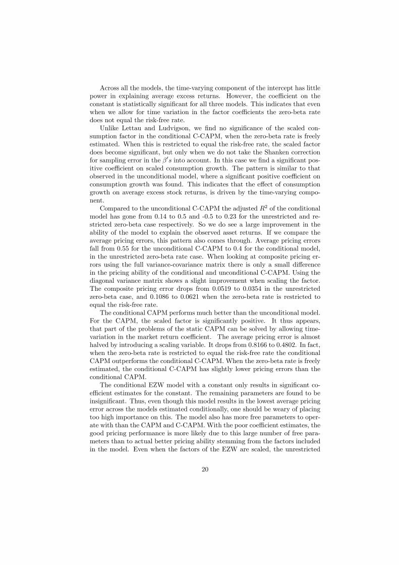
V.5 Pricing ability

To give a more visual description of the pricing capability of the models in-vestigated, the graphs presented in figure1, figure2, and figure3 show plots ofaverage realized excess returns and the average excess returns obtained fromthe respective models. Realized returns are plotted along the horizontal axisand estimated returns along the vertical axis. If a given model were to fit theempirical data perfectly, all observations would lie along the 45 line.From the plots of the four traditional models in figure 1, it is clear that

the Fama-French model has the best performance. The points are relativelyclose to the 45 line and there are no extreme outliers. It is also obvious thatthe CAPM fits the data poorly. In fact, the portfolios with the lowest realizedexcess returns obtain the highest estimated excess returns from the CAPM.These are the small growth portfolios. The extreme outliers below the 45 lineare also from the small size quantile, but are on the other end of the BE/MEspectrum as value stocks. This is the well documented value-effect, which thestatic CAPM is unable to handle. The C-CAPM does slightly better, but isstill unable to fit the realized excess return of the small growth portfolio. Asthe CAPM documents, there is little pricing ability in the market return factor.Including this along with the consumption growth factor, as is done with theEZW C-CAPM, thus results in plots closely mimicking the C-CAPM.The intertemporal models of Campbell and Vuolteenaho perform somewhat

better than the traditional C-CAPM and CAPM, as can be seen in figure 2. Inthe unrestricted case particularly, realized and estimated excess returns line uprelatively well. The restricted CV model faces some of the same problems as thestatic CAPM. Estimated excess returns for the small growth and small valuestock portfolios are very close, especially when the zero-beta rate is restrictedto equal the risk-free rate. This contradicts the empirical observations of arealized annualized excess return of 4.8% for the small growth portfolio and14.3% in the small value portfolio case. Both the CV-models have problemsfitting the small growth portfolio situated as the left most point on both plots.The models predict higher returns than the empirically realized excess return of1.2% per quarter. The best fit is found when estimating the four factor modelthat includes the VAR factors of the Campbell and Vuolteenaho I-CAPM. Theplots of portfolio returns lie very close to the 45 line and there is no value orsize effect issues. As could be expected, the more free factors, the better modelfit results.The final models investigated are the conditional CAPM and C-CAPM. As

can be seen from figure 3, there is still some dispersion in the plots around the 45

line. In comparison to the unconditional models however, a clear improvementcan be noted. Especially in the case of the CAPM. The conditional C-CAPM fitsthe small growth portfolio slightly better than the CV-models. The conditionalEZW C-CAPM without a constant also fits this portfolio relatively well, but onthe other hand has problems with the small value portfolio located at the rightmost point on the figure. There thus still seems to be some problems in fittingthe value premium.

22

VI Concluding remarksThe consumption based capital asset pricing model (C-CAPM) has had an im-portant place in the finance research literature over the past 25 years, despitethe poor empirical performance of the model. The reason it has maintained theinterest of the academic world, is the simplicity and intuitive appeal of the the-ory underlying the model. We are thus not interested in dismissing the modelcompletely. Instead focus is on the assumptions made to get from the basicidea of the priced risk of an asset being determined by the asset’s covariancewith the marginal utility of consumption, to the risk measures estimated empir-ically. Can the empirical problems of the C-CAPM be solved by revising theseassumptions?A number of alternative models attempting to improve on the pricing ability

of the C-CAPM have been developed. Two strands of the literature are inves-tigated in this paper. The intertemporal CAPM of Campbell and Vuolteenaho(2004) and the conditional C-CAPM of Cochrane (1996) and Lettau and Lud-vigson (2001b).The first model is based on the assumption that empirical consumption data

is a poor proxy for the measure of consumption referred to in the theoreticalC-CAPM. If the deviations between the theoretical and empirical measures ofconsumption are large, these data issues may be the root of the poor empiricalperformance of the C-CAPM. From this observation Campbell and Vuolteenaho(2004) develop a two beta intertemporal model, based on the same frameworkas the C-CAPM, but without reference to consumption. Instead the asset riskpremium is determined by a cash-flow and a discount-rate beta.The second set of models investigated, focus on the conditional pricing ability

of the C-CAPM. The reasoning behind this setup is recent empirical evidence oftime variation in expected returns. If the cause of this is time-varying risk prices,then we must incorporate it into the model. This can be achieved by restatingthe C-CAPM conditionally, in a scaled factor model setup. The approximatelog consumption-wealth ratio cay of Lettau and Ludvigson (2001a) is used asconditioning variable.The traditional C-CAPM, as well as the CAPM and the well known three

factor Fama-French model are estimated on quarterly US data. These are thencompared to estimates of the models from the two alternative strands of litera-ture, to investigate whether any quantifiable improvements have been made inthe empirical asset pricing ability. The assets priced are the 25 size and BE/MEsorted Fama-French portfolios.The empirical results of this paper underline previous research showing the

poor performance of the C-CAPM as well as the static CAPM. The estimatedcoefficients are insignificant or of the wrong sign, compared to that predicted bythe underlying theory. The C-CAPM has slightly lower average pricing errorsthan the CAPM, but is still unable to explain the value and size effects.Compared to the C-CAPM the intertemporal model of Campbell and Vuolteenaho

(2004) has much higher R2 and lower pricing errors. The two betas of the modeldo a better job than the traditional models of fitting the unconditional equity

23

premium. However, there are still some problems in matching the realized re-turns on the extreme small growth stock portfolio. Especially when we restrictthe price of discount-rate risk to equal the sample variance of the discount rate.When scaling the consumption growth factor of the C-CAPM to obtain an

estimate of the conditional C-CAPM, we also find improved asset pricing ability.With an unrestricted zero-beta rate, average pricing errors fall from 0.55 for theunconditional C-CAPM to 0.4 for the conditional model. However, neither theconsumption growth nor the scaled consumption growth factor are statisticallysignificant.Both the alternative models thus provide improved asset pricing ability over

the C-CAPM, but does one of the alternative theories outperform the other.Is there a clear candidate to take the place of the traditional C-CAPM. Toanswer this question, a number of weighted pricing error measures have beenestimated for the various models. Comparing the resulting observations canonly lead one to the conclusion, that there is no clear cut winner. None ofthe models from the alternative literature strands perform significantly betterthan the others. In fact, which strand results in the lowest weighted pricingerrors, is very much dependent on the weighting matrix chosen. Generally theCampbell and Vuolteenaho (2004) framework has lowest pricing errors whenusing a full variance-covariance matrix of returns or the moment matrix. Thepicture becomes more blurred when looking at average squared pricing errorsor errors weighted by the diagonal variance matrix of returns.On the basis of these observations it thus seems wise to continue the search,

as it were.

References[1] D. T. Breeden. An intertemporal asset pricing model with stochastic

consumption and investment opportunities. Journal of Financial Eco-nomics, 7:265—296, 1979.

[2] D. T. Breeden, M. R. Gibbons, and R. H. Litzenberger. Empirical test ofthe consumption-oriented CAPM. The Journal of Finance, 44(2):231—262, Jun. 1989.

[3] J. Y. Campbell. Intertemporal asset pricing without consumption data. TheAmerican Economic Review, 83(3):487—512, Jun. 1993.

[4] J. Y. Campbell. Understanding risk and return. The Journal of PoliticalEconomy, 104(2):298—345, Apr. 1996.

[5] J. Y. Campbell and R. J. Shiller. The dividend-price ratio and expecta-tions of future dividends and discount factors. The Review of FinancialStudies, 1(3):195—228, Autumn 1988.

[6] J. Y. Campbell and T. Vuolteenaho. Bad beta, good beta. The AmericanEconomic Review, 94(5):1—66, Dec 2004.

24

[7] J. H. Cochrane. A cross-sectional test of an investment-based asset pricingmodel. Journal of Political Economy, 104(3):572—621, 1996.

[8] J. H. Cochrane. Asset Pricing. Princeton University Press, 2001.

[9] E. F. Fama and K. R. French. The cross-section of expected stock returns.The Journal of Finance, 47(2):427—465, Jun. 1992.

[10] E. F. Fama and K. R. French. Common risk factors in the returns on stocksand bonds. Journal of Financial Economics, 33:3—56, 1993.

[11] E. F. Fama and J. D. MacBeth. Risk, return, and equilibrium: Empiricaltests. Journal of Political Economy, 81:607—636, May/June 1973.

[12] W. E. Ferson and C. R. Harvey. Conditioning variables and the cross sectionof stock returns. Journal of Finance, 54:1325—1360, Aug. 1999.

[13] S. Grossman, A. Melino, and R. Shiller. Estimating the continous-timeconsumption-based asset-pricing model. Journal of Business and Eco-nomic Statistics, 5(3):315—328, 1987.

[14] S. J. Grossman and R. J. Shiller. The determinants of the variability ofstock market prices. The American Economic Review, 71(2):222—227,May 1981. Papers and Proceedings of the Ninety-Third Annual Meetingof the American Economic Association.

[15] L. P. Hansen. Large sample properties of generalized method of momentsestimators. Econometrica, 50(4):1029—1054, Jul. 1982.

[16] L. P. Hansen and K. J. Singleton. Stochastic consumption, risk aversion,and the temporal behavior of asset returns. The Journal of PoliticalEconomy, 91(2):249—265, Apr. 1983.

[17] R. J. Hodrick and X. Zhang. Evaluating the specification errors of assetpricing models. Journal of Financial Economics, 62:327—376, 2001.

[18] R. Jagannathan and Z. Wang. An asymptotic theory for estimating beta-pricing models using cross-sectional regression. The Journal of Finance,53:1285—1309, Aug. 1998.

[19] N. R. Kocherlakota. The equity premium: It’s still a puzzle. Journal ofEconomic Literature, 34:42—71, March 1996.

[20] M. Lettau and S. Ludvigson. Resurrecting the (C)CAPM: A cross-sectionaltest when risk premia are time-varying. Journal of Political Economy,109(6):1238—1287, 2001.

[21] M. Lettau and S. C. Ludvigson. Consumption, aggregate wealth, and ex-pected stock returns. The Journal of Finance, 56(3):815—849, June 2001.

[22] M. Lettau and S. C. Ludvigson. Expected returns and expected dividendgrowth. Journal of Financial Economics, 76:583—626, 2005.

[23] R. E. Lucas Jr. Asset prices in an exchange economy. Econometrica,46:1429—1446, 1978.

25

[24] N. G. Mankiw and M. D. Shapiro. Risk and return: Consumption betaversus market beta. The review of Economics and Statistics, 68(3):452—459, Aug. 1986.

[25] N. G. Mankiw and S. P. Zeldes. The consumption of stockholders andnonstockholders. Journal of Financial Economics, 29:97—112, 1991.

[26] R. Mehra and E. C. Prescott. The equity premium: A puzzle. Journal ofMonetary Economics, 15:145—161, 1985.

[27] R. C. Merton. An intertemporal capital asset pricing model. Econometrica,41(5):867—887, Sep. 1973.

[28] J. Shanken. On the estimation of beta-pricing models. Review of FinancialStudies, 5(1):1—33, 1992.

[29] R. J. Shiller. Irrational Exuberance. Princeton University Press, 2000.

[30] S. Wheatley. Some tests of the consumption-based asset pricing model.Journal of Monetary Economics, 22:193—215, 1988.

26

Table 1: Summary statistics for 25 Fama-French portfolio returnsThe table presents average quarterly excess returns and standard errors for the25 Fama-French portfolios. The time series data run from the 1. quarter of1952 through the 4. quarter of 2001. Returns are measured in excess of the

3-month T-bill rate. Standard errors are in parentheses.Growth 2 3 4 Value

Small 1.1888 2.5099 2.6682 3.3000 3.5871(15.5616) (13.3429) (11.8208) (11.3130) (12.2051)

2 1.4924 2.2801 2.8382 3.0223 3.2880(14.0166) (11.7393) (10.3388) (10.2094) (10.9666)

3 1.7851 2.3729 2.3846 2.8640 3.0160(12.5797) (10.2430) (9.5581) (9.3997) (10.3032)

4 1.9518 1.8021 2.4781 2.6302 2.8606(11.4247) (9.5816) (8.8473) (8.8734) (10.3074)

Large 1.7223 1.7071 1.9978 2.0347 2.2393(9.0670) (8.0063) (7.2724) (7.8221) (8.6240)

27

Table 2: Unconditional models. Excess returns. With and without constant.The table presents λ estimates from the cross-sectional Fama-MacBeth regressions E [Ri,t+1 −Rf,t+1] = β0iλ. The test assets are the 25size and BE/ME sorted portfolios of Fama and French. Returns are measured in excess of the risk free rate. Rm is the return on theCRSP value weighted stock index and ∆c denotes consumption growth. Standard errors are presented in parentheses. The top set areuncorrected Fama-MacBeth standard errors and below are standard errors modified with the Shanken (1992) correction. Compositepricing errors, measured with both a full and a diagonal variance-covariance matrix, are presented in the bottom half of the table, inaddition to the square root of average squared pricing errors. Alpha and alpha-Shanken are χ2 tests of the hypothesis of zero-pricing

errors. Significance is measured at a 5% level.C-CAPM CAPM EZW C-CAPM Fama-French 2 factor Fama-French

constant 1.6164 3.3280 3.1784 2.9508 2.1558(0.5712)∗ (0.9317)∗ (0.9343)∗ (1.2870)∗ (0.5164)(0.6570)∗ (0.9366)∗ (1.3062)∗ (1.3331)∗ (0.5322)

Rm -0.8332 2.0682 -0.9174 1.8326 -1.1196 1.7297(1.0754) (0.6174)∗ (1.0705) (0.6010)∗ (1.3899) (0.5812)∗

(1.0795) (0.6201)∗ (1.3878) (0.6320)∗ (1.4313) (0.5824)∗

∆c 0.2691 0.7716 0.4492 0.5142(0.1798) (0.2229)∗ (0.1620)∗ (0.1609)∗

(0.2059) (0.4228) (0.2241)∗ (0.2352)∗

SMB 0.4283 0.5058 0.4417 2.0266(0.4156) (0.4164) (0.4163) (0.5424)∗

(0.4165) (0.4186) (0.4172) (0.5649)∗

HML 1.2949 1.3701 1.3160 1.2043(0.4343)∗ (0.4345)∗ (0.4343)∗ (0.4351)∗

(0.4360)∗ (0.4382)∗ (0.4357)∗ (0.4395)∗

R2 0.1758 -0.5007 0.0734 -0.8443 0.4711 -0.3621 0.7185 0.6690 0.7148 -1.3050R2adj 0.1399 -0.5007 0.0331 -0.8443 0.4230 -0.4214 0.6783 0.6389 0.6889 -1.4052

pricingerror-full 0.3874 0.7005 0.3511 0.4623 0.4313 0.5389 0.3062 0.3815 0.3180 0.5350pricingerror-diag 0.0519 0.1086 0.0808 0.1211 0.0458 0.0893 0.0211 0.0250 0.0213 0.2300Shanken 1.3230 3.6562 1.0106 1.0650 1.9547 2.1878 1.0785 1.1606 1.0622 1.1888alpha 71.13∗ 97.67∗ 69.51∗ 92.38∗ 68.73∗ 90.43∗ 59.67∗ 75.90∗ 62.55∗ 94.04∗

alpha-Shanken 53.76∗ 26.71 68.79∗ 86.74∗ 35.16 41.33∗ 55.62∗ 65.39∗ 58.89∗ 79.11∗

Average pricing error 0.5459 0.7366 0.5788 0.8166 0.4373 0.7018 0.3190 0.3459 0.3211 0.9129H-J dist 0.5413 0.7677 0.5277 0.5695 0.6070 0.6477 0.4908 0.5382 0.4961 0.640728

Table 3: Unconditional models. Excess returns. With and without constant.The table presents λ estimates from the cross-sectional Fama-MacBeth regressions E [Ri,t+1 −Rf,t+1] = β0iλ. The test assets are the 25size and BE/ME sorted portfolios of Fama and French. Returns are measured in excess of the risk free rate. Rm is the return on theCRSP value weighted stock index and ∆c denotes consumption growth. Standard errors are presented in parentheses. The top set areuncorrected Fama-MacBeth standard errors and below are standard errors modified with the Shanken (1992) correction. Compositepricing errors, measured with both a full and a diagonal variance-covariance matrix, are presented in the bottom half of the table, inaddition to the square root of average squared pricing errors. Alpha and alpha-Shanken are χ2 tests of the hypothesis of zero-pricing

errors. Significance is measured at a 5% level. Sample limited to Lettau and Ludvigson (2001) sample.

C-CAPM CAPM EZW C-CAPM Fama-French

constant 1.6757 2.8924 3.2824 0.3665(0.6513)∗ (0.9398)∗ (0.9240)∗ (1.4742)(0.7014)∗ (0.9421)∗ (1.2058)∗ (1.5851)

Rm -0.5755 1.8251 -1.1505 1.6451 1.3198 1.6759(1.1767) (0.7346)∗ (1.1306) (0.7101)∗ (1.6306) (0.6950)∗

(1.1786) (0.7368)∗ (1.3572) (0.7178)∗ (1.7319) (0.6960)∗

∆c 0.1892 0.6893 0.3821 0.2868(0.1911) (0.2722) (0.1707)∗ (0.1736)(0.2052) (0.4772) (0.2202)∗ (0.2029)

SMB 0.4282 0.4373(0.5083) (0.5099)(0.5093) (0.5114)

HML 1.3571 1.3556(0.4535)∗ (0.4532)∗

(0.4553)∗ (0.4554)∗

R2 0.1102 -0.7834 0.0334 -0.5669 0.3386 -0.4072 0.7507 0.7502R2adj 0.0716 -0.7834 -0.0086 -0.5669 0.2784 -0.4072 0.7150 0.7257

pricingerror-full 0.7163 0.9349 0.4924 0.5634 0.6428 0.6030 0.4459 0.4543pricingerror-diag 0.2612 0.1526 0.0936 0.1198 0.0698 0.1055 0.0221 0.0219Shanken 1.1597 3.1183 1.0049 1.049 1.7027 1.3854 1.1561 1.1896alpha 69.03∗ 84.77∗ 68.77∗ 79.99∗ 68.70∗ 79.39∗ 60.60∗ 64.19∗

alpha-Shanken 59.53∗ 27.19∗ 68.44∗ 76.24∗ 40.35∗ 57.31∗ 52.42∗ 53.96∗

Average pricing error 0.6225 0.8813 0.6488 0.8261 0.5367 0.7823 0.3295 0.3298H-J dist 0.6038 0.8710 0.6042 0.6060 0.7302 0.6448 0.5730 0.577929

Table 4: Market return beta estimates from Fama-French modelThe table presents time-series estimates of the market return beta of theFama-French 3 factor model for the 25 size and BE/ME sorted portfolios of

Fama and French.bβRm Growth 2 3 4 Value Value-GrowthSmall 0.9998 0.9929 0.9061 0.9128 0.9975 -0.0023

(0.0520) (0.0343) (0.0327) (0.0281) (0.0301)2 1.0776 1.0059 0.9649 0.9934 1.0467 -0.0309

(0.0336) (0.0285) (0.0262) (0.0261) (0.0255)3 1.0803 1.0065 0.9924 1.0107 1.0329 -0.0474

(0.0292) (0.0282) (0.9924) (0.0301) (0.0318)4 1.0522 1.0271 1.0098 1.0119 1.1042 0.0520

(0.0280) (0.0336) (0.0311) (0.0303) (0.0403)Large 1.0505 1.0008 0.9209 1.0188 1.0646 0.0141

(0.0224) (0.0269) (0.0309) (0.0287) (0.0370)Large-Small 0.0507 0.0079 0.0148 0.1060 0.0671

30

Table 5: Unconditional models. Excess returns. With and withour constant.The table presents λ estimates from the cross-sectional Fama-MacBethregressions E [Ri,t+1 −Rf,t+1] = β0iλ. The test assets are the 25 size and

BE/ME sorted portfolios of Fama and French. Returns are measured in excessof the risk-free rate. Rm is the return on the CRSP value weighted stock

index, NCF and NDR are the two I-CAPM factors developed by Campbell andVuolteenaho (2004), TY is the bond yield spread, PE is the price earnings

ratio, and V S is the value spread. Standard errors are presented inparentheses. The top set are uncorrected Fama-MacBeth standard errors andbelow are standard errors modified with the Shanken (1992) correction.Composite pricing errors, measured with both a full and a diagonal

variance-covariance matrix, are presented in the bottom half of the table, inaddition to the square root of average squared pricing errors. Alpha andalpha-Shanken are χ2 tests of the hypothesis of zero-pricing errors.

Significance is measured at a 5% level.CV-unrestricted CV-restricted VAR factors

constant -0.3556 -1.7015 0.9538(1.4144) (1.1359) (1.3318)(1.8788) (1.0114) (2.3704)

Rm 0.9101 1.7891(1.4440) (0.5904)∗

(2.4273) (0.6312)∗

NCF 2.7391 2.5481 3.1254 1.5932(0.8819)∗ (0.5463)∗ (0.8429)∗ (0.6167)∗

(1.1549)∗ (0.6792)∗ (1.0871)∗ (0.3983)∗

NDR -0.2130 -0.3531 0.6828 0.6828(1.1387) (0.8083)(1.4237) (0.9264)

TY 0.7376 0.7192(0.1786)∗ (0.1919)∗

(0.3118)∗ (0.3549)∗

PE 0.2029 0.2529(0.1083) (0.0745)∗

(0.1895) (0.1350)V S -0.0055 -0.0210

(0.0238) (0.0304)(0.0400) (0.0552)

R2 0.5765 0.5735 0.5027 0.3314 0.8530 0.8284R2adj 0.5380 0.5549 0.4811 0.3314 0.8236 0.8038pricingerror-full 0.3731 0.3581 0.4347 0.3551 0.2683 0.3085pricingerror-diag 0.0320 0.0330 0.0329 0.0402 0.0124 0.0139Shanken 1.7644 1.6568 1.9686 1.2517 3.1679 3.5419alpha 62.08∗ 69.82∗ 68.05∗ 70.45∗ 46.63∗ 56.72∗

alpha-shanken 35.19 42.14∗ 36.68 57.68∗ 14.72 16.01Average pricing error 0.3913 0.3927 0.4240 0.4917 0.2304 0.2491H-J dist. 0.5526 0.5400 0.5942 0.5145 0.4865 0.5214

31

Table 6: Beta estimates from Campbell modelbβCF Growth 2 3 4 Value Value-GrowthSmall 0.9986 1.0504 1.0495 1.1404 1.2779 0.2793

(0.2260) (0.1869) (0.1709) (0.1613) (0.1869)2 0.9407 0.9848 1.1201 1.1724 1.2754 0.3347

(0.1786) (0.1537) (0.1316) (0.1393) (0.1596)3 0.8067 1.0760 1.1878 1.2546 1.3058 0.4991

(0.1448) (0.1205) (0.1174) (0.1235) (0.1493)4 0.9563 1.0727 1.2481 1.2319 1.3603 0.4040

(0.1181) (0.1045) (0.1002) (0.1031) (0.1456)Large 0.6866 0.9042 0.9602 1.0988 1.0079 0.3213

(0.0773) (0.0823) (0.0855) (0.0991) (0.1297)Large-Small -0.312 -0.1462 -0.0893 -0.0416 -0.2700bβDR Growth 2 3 4 Value Value-GrowthSmall 1.4726 1.2857 1.1078 1.0600 1.0744 -0.3982

(0.0869) (0.0718) (0.0657) (0.0620) (0.0718)2 1.4273 1.1724 1.0287 0.9700 0.9935 -0.4338

(0.0687) (0.0591) (0.0506) (0.0535) (0.0613)3 1.3350 1.0584 0.9510 0.8907 0.9213 -0.4137

(0.0556) (0.0463) (0.0451) (0.0475) (0.0574)4 1.2460 1.0113 0.8911 0.8874 0.9323 -0.3137

(0.0454) (0.0402) (0.0385) (0.0396) (0.0559)Large 1.0325 0.8595 0.7305 0.7484 0.7591 -0.2734

(0.0297) (0.0316) (0.0329) (0.0381) (0.0498)Large-Small -0.4401 -0.4262 -0.3773 -0.3116 -0.3153

32

Table 7: Conditional models. Excess returns. With and without constant.The table presents λ estimates from the cross sectional Fama-MacBethregressions E [Ri,t+1 −Rf,t+1] = β0iλ. The test assets are the 25 size and

BE/ME sorted portfolios of Fama and French. Returns are measured in excessof the risk-free rate. Rm,t+1 is the return on the CRSP value weighted stock

index and ∆ct+1 denotes consumption growth. cayt is the laggedconsumption-wealth ratio proxy, used as scaling variable in the conditionalmodels. Standard errors are presented in parentheses. The top set are

uncorrected Fama-MacBeth standard errors and below are standard errorsmodified with the Shanken (1992) correction. Composite pricing errors,measured with both a full and a diagonal variance-covariance matrix, arepresented in the bottom half of the table, in addition to the square root ofaverage squared pricing errors. Alpha and alpha-Shanken are χ2 tests of thehypothesis of zero-pricing errors. Significance is measured at a 5% level.

Conditional C-CAPM Conditional CAPM Conditional EZW C-CAPMconstant 2.8500 1.9016 2.0048

(0.8173)∗ (0.8472)∗ (0.8383)∗

(1.0625)∗ (1.2083) (1.0166)∗dcayt -0.2116 -0.9892 -0.3020(0.3252) (0.4852)∗ (0.3463)(0.4165) (0.6861) (0.4156)

Rm,t+1 -0.0378 1.8666 -0.0222 1.8161(1.0139) (0.6190)∗ (1.0119) (0.6053)∗

(1.3231) (0.6505)∗ (1.1624) (0.6264)∗dcayt ∗Rm,t+1 5.0295 7.6996 2.1602 4.9324(1.9549)∗ (1.9358)∗ (1.8665) (2.2634)∗

(2.7203) (2.4860)∗ (2.2161) (2.8928)∆ct+1 0.1422 0.0664 0.1291 0.1552

(0.1939) (0.2281) (0.1166) (0.1765)(0.2505) (0.4737) (0.1395) (0.2281)dcayt ∗∆ct+1 0.3779 1.4422 0.1911 0.3234(0.2481) (0.3930)∗ (0.2195) (0.2207)(0.3190) (0.8163) (0.2633) (0.2834)

R2 0.5686 0.2638 0.5014 0.3620 0.5957 0.5131R2adj 0.5070 0.2318 0.4301 0.3342 0.4893 0.4435Pricingerror-full 0.3990 0.6910 0.5628 0.6006 0.4242 0.5426Pricingerror-diag 0.0354 0.0621 0.0362 0.0475 0.0306 0.0367Shanken 1.6900 4.3858 2.0339 1.7383 1.4706 1.6948alpha 69.21∗ 92.60∗ 69.05∗ 91.48∗ 66.86∗ 87.40∗

alpha-shanken 40.95∗ 21.11 33.95 52.63∗ 45.46∗ 51.57∗

Average pricing error 0.3950 0.5159 0.4246 0.4803 0.3824 0.4196H-J dist. 0.5780 0.7762 0.6838 0.6940 0.5873 0.6611

33

Figure 1: Pricing performance of traditional modelsIn the four figures below, returns for the traditional models are presented.

Realized sample average excess returns are on the x-axis and predicted excessreturns are along the y-axis. Each figure plots excess returns for the 25Fama-French portfolios. Two model versions are presented in each figure.Squares represent estimates for the version with the zero-beta rate restrictedto equal the risk-free rate and circles give estimates where the zero-beta rate is

freely estimated.

43210

4

3

2

1

0

C-CAPM

43210

4

3

2

1

0

CAPM

43210

4

3

2

1

0

EZW C-CAPM

43210

4

3

2

1

0

Fama-French

34

Figure 2: Pricing performance of I-CAPMIn the three figures below, returns for the Campbell and Vuolteenaho modelsare presented. Realized sample average excess returns are on the x-axis andpredicted excess returns are along the y-axis. Each figure plots excess returnsfor the 25 Fama-French portfolios. Two model versions are presented in eachfigure. Squares represent estimates for the version with the zero-beta raterestricted to equal the risk-free rate and circles give estimates where the

zero-beta rate is freely estimated.

43210

4

3

2

1

0

CV model, unrestricted

43210

4

3

2

1

0

CV model, restricted

43210

4

3

2

1

0

VAR Factor model

35

Figure 3: Pricing performance of conditional modelsIn the three figures below, returns for the conditional models are presented.Realized sample average excess returns are on the x-axis and predicted excessreturns are along the y-axis. Each figure plots excess returns for the 25Fama-French portfolios. Two model versions are presented in each figure.Squares represent estimates for the version with the zero-beta rate restrictedto equal the risk-free rate and circles give estimates where the zero-beta rate is

freely estimated.

43210

4

3

2

1

0

Conditional C-CAPM

43210

4

3

2

1

0

Conditional CAPM

43210

4

3

2

1

0

Conditional EZW C-CAPM

36