improving the e ciency of selection in a plant breeding
TRANSCRIPT

Improving the efficiency of
selection in a plant breeding
program using information on
correlated traits, ancestry and
environments.
Aanandini Ganesalingam
Bachelor of Science (Agriculture) (Hons) & Bachelor of Economics
This thesis is presented for the degree of
Doctor of Philosophy
of
The University of Western Australia
School of Plant Biology & The UWA Institute of Agriculture
2013

ii
Abstract
This thesis presents how information on correlated traits, ancestry and envi-
ronments can be used within a mixed model framework to improve selection
in plant breeding. The motivating example is canola (Brassica napus L.).
Plant survival data in blackleg disease of canola are often composed of
multiple measures used to form a derived variable, such as percent survival
values, which is then subject to analysis. Instead, a bivariate linear mixed
model approach is proposed in which the two variables are the initial and
final plant counts. This approach is demonstrated using data from blackleg
disease nurseries in the 2009 growing season in Australia. The counts were
considered as two ‘traits’, which are affected by different biological, genetic
and environmental influences. The bivariate mixed model approach for the
analysis of plant survival data not only provided a more detailed picture
but also a more accurate assessment of the impact of disease resistance
compared with the univariate analysis of percentage survival data.
The release of new cultivars onto the market is preceded by extensive test-
ing of varieties across target environments and growing seasons in multi-
environment trials (METs), which is a core process in plant breeding. An-
other related objective is the selection of parents for the next cycle of breed-
ing. The inclusion of pedigree information in the MET analysis satisfies
both objectives.
Using the 2011 subset of data from a canola breeding program, this thesis
demonstrates the use of spatial analysis of individual trials and then extends
this to an across site analysis using a MET and factor analytic (FA) mixed
model framework. The efficiency of this process is demonstrated in the
iii

spatial analysis of individual trials to control within trial environmental im-
pacts when pedigree information is included. The study demonstrates that
pedigree information aids in the modeling of spatial errors and identification
of outliers by adding information for entry performance from relatives. The
study concludes that base-line non-genetic modeling should always include
pedigree information for the determination of site-specific spatial models,
especially in the case of p-rep trial designs, which are commonly used in
plant breeding programs for the testing of early generation entries.
The extension of the single site pedigree analysis to a MET/FA analy-
sis examines how environments impact on entry performance (genotype by
environment interaction) within a breeding program. The MET/FA with
pedigree information not only enables independent estimation of additive
and non-additive genetic effect of entries, but also the impact of GxE on
these genetic effects. This study also derived total genetic variance for
hybrid and non-hybrid entries, to observe the impact of GxE on these dif-
fering entry types. While the estimated genetic correlations resulting from
MET/FA analysis did not indicate different patterns of GxE for hybrid or
non-hybrid entry types, it is a more accurate selection tool given the dif-
ferences in inbreeding levels between entry types. In other plant breeding
datasets that jointly trial hybrid and non-hybrid entries it may indicate
broad insights into the basis of possible sources of GxE on trial groupings.
Finally a topic of interest that arose during the research of this thesis is
the extensive time to analysis completion in MET/FA with pedigree model.
This chapter investigated the algorithm employed in ASReml-R and the
time required for the completion of a single iteration for different genetic
variance models alongside different lengths of data sets with correspond-
ing pedigree files. While it was observed that iteration completion times
increased substantially when pedigree information is included in MET/FA
analysis, the findings of this chapter also indicate that a so-called Reduced
Rank + diagonal formulation of the FA model took a third of the time
for the completion of the second iteration completion than the standard
formulation.
iv

The outcomes of research from this thesis have implications for all plant
breeding programs whether hybrid or self-pollinated crops.
v

vi

Acknowledgements
“Not all those who wander are lost.”
-J.R.R Tolkien
To my supervisor Alison, I am indebted to you for your patience with my
wandering given that I didn’t really know what I signed up for. I am most
grateful for your ability to make any mixed model analysis look ‘simple’ and
for teaching me most of the mixed model theory from scratch. I would also
like to acknowledge Brian Cullis, who deserves the credit of a supervisor,
with his steady input, ideas and discussions during the length of this PhD.
Alison and Brian, your guidance, motivation (and perseverance!) with me
for the last three and a bit years shaped this thesis. I owe both of you my
deepest gratitude, as this thesis wouldn’t have been completed without such
an excellent supervisory tag-team.
To my two supervisors at UWA. Thanks Wallace for providing me with
the CBWA data set, reading the numerous drafts of this thesis and co-
ordinating my thesis. Thanks Cameron for putting me on this path, when
you unwittingly hired to me to do casual work at CBWA all those years
ago.
I would also like to thank Dr. Ed Roumen for providing me with the oppor-
tunity to undertake this PhD in the first place and for your numerous and
stimulating discussions in the initial stages. I would also like to acknowl-
edge Bayer Crop Science for providing me with the scholarship to undertake
this PhD and the Mike Carroll travel fellowship for providing the financial
assistance and opportunity to undertake research at Rothamsted Research.
vii

To my friends at UWA who shared this journey with me, Annaliese, An-
nisa, Caroline, Christine and Maggie, the biggest thank-you is owed. You
girls were not only my support group but ensured that I was motivated
(caffeinated) for work on a daily basis. Special mention and thanks here to
Emily for making the stay at Rothamsted and trips to Tumut an absolute
blast.
Thanks to papa and mame for your love and support, especially for putting
up with me being a perpetual (and often absent) student. Last but not least,
I would also like to thank my husband, Hari for his unwavering support,
understanding and patience during the ups and downs of this journey; I
could not have done this without you, I dedicate this thesis to you.
viii

Statement of original contribution
This thesis has been completed during the course of enrollment in a PhD
degree at the University of Western Australia, and has not been used pre-
viously for a degree or diploma at any other institution. To the best of
my knowledge and belief, this thesis does not contain material previously
published or written by another person, except where due reference is made
in the text of the thesis.
Aanandini Ganesalingam
May, 2013
ix

x

Contents
List of Figures xvii
List of Tables xxi
Glossary xxiii
1 Introduction 1
2 Literature Review - Methods of measurement and analysis of plant
survival data sets 5
2.1 Introduction . . . . . . . . . . . . . . . . . . . . . . . . . . . . . . . . . . 5
2.2 Measures of disease . . . . . . . . . . . . . . . . . . . . . . . . . . . . . . 6
2.3 Blackleg disease incidence . . . . . . . . . . . . . . . . . . . . . . . . . . 6
2.4 Bivariate analysis . . . . . . . . . . . . . . . . . . . . . . . . . . . . . . . 9
2.4.1 Biological motivations . . . . . . . . . . . . . . . . . . . . . . . . 9
2.4.2 Statistical motivations . . . . . . . . . . . . . . . . . . . . . . . . 11
2.5 Summary . . . . . . . . . . . . . . . . . . . . . . . . . . . . . . . . . . . 13
3 A bivariate mixed model approach for the analysis of plant survival
data 15
3.1 Data set description . . . . . . . . . . . . . . . . . . . . . . . . . . . . . 16
3.2 Measuring disease incidence . . . . . . . . . . . . . . . . . . . . . . . . . 17
3.3 Univariate analysis . . . . . . . . . . . . . . . . . . . . . . . . . . . . . . 18
3.3.1 Statistical model . . . . . . . . . . . . . . . . . . . . . . . . . . . 18
3.3.2 Checking the adequacy of the spatial model . . . . . . . . . . . . 20
3.3.3 Estimation and Fitting . . . . . . . . . . . . . . . . . . . . . . . 20
xi

CONTENTS
3.3.4 Univariate analysis results . . . . . . . . . . . . . . . . . . . . . . 21
3.3.4.1 York disease nursery . . . . . . . . . . . . . . . . . . . . 21
3.3.4.2 All disease nurseries . . . . . . . . . . . . . . . . . . . . 25
3.4 Bivariate analysis . . . . . . . . . . . . . . . . . . . . . . . . . . . . . . . 27
3.4.1 Statistical model . . . . . . . . . . . . . . . . . . . . . . . . . . . 27
3.4.2 Model Comparisons . . . . . . . . . . . . . . . . . . . . . . . . . 29
3.4.3 Bivariate analysis results . . . . . . . . . . . . . . . . . . . . . . 30
3.4.3.1 York disease nursery . . . . . . . . . . . . . . . . . . . . 30
3.4.3.2 All disease nurseries . . . . . . . . . . . . . . . . . . . . 34
3.5 Discussion . . . . . . . . . . . . . . . . . . . . . . . . . . . . . . . . . . . 39
3.6 Summary . . . . . . . . . . . . . . . . . . . . . . . . . . . . . . . . . . . 42
4 Further applications of bivariate analysis for plant breeding data 45
4.1 Introduction . . . . . . . . . . . . . . . . . . . . . . . . . . . . . . . . . . 45
4.2 Breeding for disease resistance . . . . . . . . . . . . . . . . . . . . . . . 46
4.2.1 Adjustment for seedling emergence . . . . . . . . . . . . . . . . . 47
4.2.2 Adjustment for heading date . . . . . . . . . . . . . . . . . . . . 47
4.2.3 Adjustment for fungal mould levels . . . . . . . . . . . . . . . . . 48
4.2.4 Adjustment for plant stand and days from planting . . . . . . . . 49
4.3 Breeding for grain yield . . . . . . . . . . . . . . . . . . . . . . . . . . . 50
4.3.1 Adjustment for plant stand . . . . . . . . . . . . . . . . . . . . . 50
4.3.2 Adjustment for grain moisture levels . . . . . . . . . . . . . . . . 51
4.4 QTL analysis - adjusting for other traits . . . . . . . . . . . . . . . . . . 52
4.5 Discussion . . . . . . . . . . . . . . . . . . . . . . . . . . . . . . . . . . . 55
4.6 Summary . . . . . . . . . . . . . . . . . . . . . . . . . . . . . . . . . . . 56
5 Literature Review - Pedigree information in plant breeding METs 57
5.1 Introduction . . . . . . . . . . . . . . . . . . . . . . . . . . . . . . . . . . 57
5.2 Analysis of MET trials . . . . . . . . . . . . . . . . . . . . . . . . . . . . 61
5.2.1 Linear Mixed Model Approach . . . . . . . . . . . . . . . . . . . 61
5.2.1.1 Prediction models and relationship matrices . . . . . . 63
5.3 Heterosis and GxE . . . . . . . . . . . . . . . . . . . . . . . . . . . . . . 63
5.4 Relationship Information . . . . . . . . . . . . . . . . . . . . . . . . . . . 64
5.4.1 Pedigree based estimators of COF . . . . . . . . . . . . . . . . . 65
xii

CONTENTS
5.4.2 Molecular marker based estimators . . . . . . . . . . . . . . . . . 67
5.4.3 Higher order interactions . . . . . . . . . . . . . . . . . . . . . . 70
5.5 Conclusion and further research . . . . . . . . . . . . . . . . . . . . . . . 71
6 Canola multi-environment trial data set 73
6.1 Data set description . . . . . . . . . . . . . . . . . . . . . . . . . . . . . 73
6.2 Pedigree Information . . . . . . . . . . . . . . . . . . . . . . . . . . . . . 75
7 Spatial analysis (N-gen modelling) of trials with pedigree information 81
7.1 Introduction . . . . . . . . . . . . . . . . . . . . . . . . . . . . . . . . . . 81
7.2 Methods and Materials . . . . . . . . . . . . . . . . . . . . . . . . . . . . 83
7.2.1 Data set description . . . . . . . . . . . . . . . . . . . . . . . . . 83
7.2.1.1 Superblock design component . . . . . . . . . . . . . . 84
7.2.2 Single Trial analysis . . . . . . . . . . . . . . . . . . . . . . . . . 85
7.2.2.1 Standard statistical model . . . . . . . . . . . . . . . . 85
7.2.2.2 Pedigree statistical model . . . . . . . . . . . . . . . . . 86
7.2.3 Ngen variance modeling . . . . . . . . . . . . . . . . . . . . . . . 87
7.2.4 Outlier detection . . . . . . . . . . . . . . . . . . . . . . . . . . . 88
7.2.5 Analysis . . . . . . . . . . . . . . . . . . . . . . . . . . . . . . . . 88
7.2.6 Estimation and Fitting . . . . . . . . . . . . . . . . . . . . . . . 89
7.3 Results . . . . . . . . . . . . . . . . . . . . . . . . . . . . . . . . . . . . . 89
7.3.1 Ngen variance modeling - York trial . . . . . . . . . . . . . . . . 89
7.3.1.1 Model parameters . . . . . . . . . . . . . . . . . . . . . 97
7.3.2 All trials . . . . . . . . . . . . . . . . . . . . . . . . . . . . . . . . 99
7.4 Discussion . . . . . . . . . . . . . . . . . . . . . . . . . . . . . . . . . . . 101
7.5 Summary . . . . . . . . . . . . . . . . . . . . . . . . . . . . . . . . . . . 104
8 MET analysis of trials with pedigree information 105
8.1 Introduction . . . . . . . . . . . . . . . . . . . . . . . . . . . . . . . . . . 105
8.2 Methods and Materials . . . . . . . . . . . . . . . . . . . . . . . . . . . . 106
8.2.1 Description of data . . . . . . . . . . . . . . . . . . . . . . . . . . 106
8.2.2 Statistical models . . . . . . . . . . . . . . . . . . . . . . . . . . 110
8.2.3 Model fitting and examination of GxE . . . . . . . . . . . . . . . 112
8.3 Results . . . . . . . . . . . . . . . . . . . . . . . . . . . . . . . . . . . . . 113
xiii

CONTENTS
8.3.1 N-gen variance modeling . . . . . . . . . . . . . . . . . . . . . . . 113
8.3.2 Outliers . . . . . . . . . . . . . . . . . . . . . . . . . . . . . . . . 115
8.3.3 FA Model . . . . . . . . . . . . . . . . . . . . . . . . . . . . . . . 115
8.3.4 GxE for additive effects . . . . . . . . . . . . . . . . . . . . . . . 116
8.3.5 GxE for non-additive effects . . . . . . . . . . . . . . . . . . . . . 119
8.3.6 GxE for total genetic effects . . . . . . . . . . . . . . . . . . . . 123
8.3.6.1 Total genetic effects: all entries . . . . . . . . . . . . . . 123
8.3.6.2 Total genetic effects: hybrid entries & non-hybrid entries 124
8.3.7 Selection . . . . . . . . . . . . . . . . . . . . . . . . . . . . . . . 127
8.3.7.1 Commercial selection . . . . . . . . . . . . . . . . . . . 127
8.3.7.2 Selection for parents . . . . . . . . . . . . . . . . . . . . 130
8.4 Discussion . . . . . . . . . . . . . . . . . . . . . . . . . . . . . . . . . . . 132
8.5 Summary . . . . . . . . . . . . . . . . . . . . . . . . . . . . . . . . . . . 138
9 Analysis completion times: MET analysis with pedigree information 141
9.1 Introduction . . . . . . . . . . . . . . . . . . . . . . . . . . . . . . . . . . 141
9.2 Computation background . . . . . . . . . . . . . . . . . . . . . . . . . . 143
9.2.1 Independent formulation . . . . . . . . . . . . . . . . . . . . . . . 143
9.2.1.1 Toy example . . . . . . . . . . . . . . . . . . . . . . . . 144
9.2.2 Dependent formulation . . . . . . . . . . . . . . . . . . . . . . . 147
9.2.2.1 Toy Example . . . . . . . . . . . . . . . . . . . . . . . 148
9.2.3 Reduced rank version - dependent formulation . . . . . . . . . . 150
9.2.3.1 Toy Example . . . . . . . . . . . . . . . . . . . . . . . . 150
9.2.4 Absorption . . . . . . . . . . . . . . . . . . . . . . . . . . . . . . 153
9.2.5 Sparsity and ordering . . . . . . . . . . . . . . . . . . . . . . . . 153
9.3 Example: Analysis completion times . . . . . . . . . . . . . . . . . . . . 158
9.3.1 The data set . . . . . . . . . . . . . . . . . . . . . . . . . . . . . 158
9.3.2 Analysis . . . . . . . . . . . . . . . . . . . . . . . . . . . . . . . . 159
9.3.3 Computation . . . . . . . . . . . . . . . . . . . . . . . . . . . . . 159
9.3.4 Results & Discussion . . . . . . . . . . . . . . . . . . . . . . . . . 159
9.3.5 Summary . . . . . . . . . . . . . . . . . . . . . . . . . . . . . . . 162
10 General Discussion 163
10.1 Introduction . . . . . . . . . . . . . . . . . . . . . . . . . . . . . . . . . . 163
xiv

CONTENTS
10.2 Correlated traits . . . . . . . . . . . . . . . . . . . . . . . . . . . . . . . 164
10.3 Ancestry & Environments . . . . . . . . . . . . . . . . . . . . . . . . . . 166
10.4 Future directions of research: correlated traits, ancestry and environments170
10.5 Conclusion . . . . . . . . . . . . . . . . . . . . . . . . . . . . . . . . . . 171
Appendices 173
A Published paper based on Chapter 3 175
B ASReml-R Code 189
B.1 ASReml-R Code for fitting the univariate trait models in Chapter 3 . . 189
B.2 ASReml-R Code for fitting the bivariate trait models in Chapter 3 . . . 190
Bibliography 191
xv

CONTENTS
xvi

List of Figures
1.1 Canola production regions across southern Australia . . . . . . . . . . . 2
2.1 The lifecycle of blackleg disease . . . . . . . . . . . . . . . . . . . . . . . 7
3.1 Location of blackleg disease nurseries across Australia . . . . . . . . . . 16
3.2 York disease nursery initial plot of residuals and sample variogram . . . 23
3.3 York disease nursery final plot of residuals and sample variogram . . . . 24
3.4 Plot of predicted entry means at maturity against emergence. . . . . . . 32
3.5 Plot of the difference between predicted entry means at maturity and
emergence against emergence . . . . . . . . . . . . . . . . . . . . . . . . 33
3.6 Plot of the difference between predicted entry means at maturity and
emergence against emergence at Shenton Park disease nursery . . . . . . 36
3.7 Plot of the difference between predicted entry means at maturity and
emergence against emergence at Wagga Wagga disease nursery . . . . . 37
5.1 Schematic representation of two entries (blue = entry 1 and pink =
entry 2) and their performance across two environments: (a) no GxE;
(b) GxE due to heterogeneity of variance between the environments but
not lack of genetic correlation; (c) GxE due to lack of genetic correlation
but not heterogeneity of variance between environments; (d) GxE due
to heterogeneity of variance between the environments and the lack of
genetic correlation. This diagram has been reproduced from Cooper
et al. (1996). . . . . . . . . . . . . . . . . . . . . . . . . . . . . . . . . . 59
6.1 Location of multi-environment trials across Australia . . . . . . . . . . . 74
xvii

LIST OF FIGURES
7.1 Initial plot of residuals and sample variogram for N-gen models fitted for
standard and pedigree models for the York trial. . . . . . . . . . . . . . 91
7.2 Initial plots of faces of the sample variogram (solid line) and the simu-
lation mean (dotted line) as banded by 95% coverage intervals (dashed
lines) for standard and pedigree models at the York trial. . . . . . . . . 92
7.3 Plot of residuals and sample variogram for N-gen models fitted for stan-
dard and pedigree models after the addition of linear regression on row
number at the York trial. . . . . . . . . . . . . . . . . . . . . . . . . . . 93
7.4 Plots of faces of the sample variogram (solid line) and the simulation
mean (dotted line) as banded by 95% coverage intervals (dashed lines)
for standard and pedigree models after the addition of linear regression
on row number at the York trial. . . . . . . . . . . . . . . . . . . . . . . 94
7.5 Plot of residuals and sample variogram for N-gen models for standard
and pedigree models after the addition of random column effects for the
York trial. . . . . . . . . . . . . . . . . . . . . . . . . . . . . . . . . . . . 95
7.6 Plots of faces of the sample variogram (solid line) and the simulation
mean (dotted line) as banded by 95% coverage intervals (dashed lines)
for standard and pedigree models after the addition of random column
effects at the York trial. . . . . . . . . . . . . . . . . . . . . . . . . . . . 96
7.7 Outliers detected under standard and pedigree models . . . . . . . . . . 100
8.1 Dendrogram of the dissimilarity matrix (It−Cea) of additive effects for
yield. . . . . . . . . . . . . . . . . . . . . . . . . . . . . . . . . . . . . . . 117
8.2 Heatmap of the REML estimate of the additive genetic correlation ma-
trix (Cea) . . . . . . . . . . . . . . . . . . . . . . . . . . . . . . . . . . . 118
8.3 Dendrogram of the dissimilarity matrix (It −Cei) of trial non-additive
genetic effects for yield . . . . . . . . . . . . . . . . . . . . . . . . . . . . 120
8.4 Heatmap of the REML estimate of non-additive genetic correlation ma-
trix (Cei) . . . . . . . . . . . . . . . . . . . . . . . . . . . . . . . . . . . 121
8.5 Heatmap of the REML estimate of the total genetic correlation matrix
(Ceg, where a = 1.82) . . . . . . . . . . . . . . . . . . . . . . . . . . . . 124
8.6 Total genetic C-BLUPs for hybrid entries from Cluster 2 plotted against
Cluster 1 . . . . . . . . . . . . . . . . . . . . . . . . . . . . . . . . . . . 128
xviii

LIST OF FIGURES
8.7 Total genetic C-BLUPs for non-hybrid entries from Cluster 2 plotted
against Cluster 1 . . . . . . . . . . . . . . . . . . . . . . . . . . . . . . . 129
8.8 Additive genetic C-BLUPs for non-hybrid entries from Cluster 2 plotted
against Cluster 1 . . . . . . . . . . . . . . . . . . . . . . . . . . . . . . . 131
9.1 Toy example of the independent formulation . . . . . . . . . . . . . . . . 146
9.2 Toy example of dependent formulation . . . . . . . . . . . . . . . . . . . 149
9.3 Toy example of RR version of dependent formulation . . . . . . . . . . . 152
9.4 Sparsity after absorption in a toy example of the dependent formulation
with correct ordering . . . . . . . . . . . . . . . . . . . . . . . . . . . . . 155
9.5 Sparsity after absorption in a toy example of the dependent formulation
with incorrect ordering . . . . . . . . . . . . . . . . . . . . . . . . . . . . 156
9.6 Second iteration completion times . . . . . . . . . . . . . . . . . . . . . 161
xix

LIST OF FIGURES
xx

List of Tables
3.1 Location based summaries of the 2009 blackleg disease nurseries . . . . 17
3.2 Description of 2009 blackleg disease nursery experiments . . . . . . . . . 17
3.3 Spatial modeling in univariate analyses of emergence and maturity trait
data for each experiment . . . . . . . . . . . . . . . . . . . . . . . . . . . 26
3.4 REML estimates of error variance from the univariate and bivariate mod-
els at each disease nursery. . . . . . . . . . . . . . . . . . . . . . . . . . . 35
3.5 REML estimates of entry variance from the univariate and bivariate
models at each disease nursery. . . . . . . . . . . . . . . . . . . . . . . . 35
3.6 Accuracy of prediction for univariate and bivariate models . . . . . . . . 38
6.1 Details of multi-environment trials in the canola data set . . . . . . . . 75
6.2 Summary of individual trial details from the canola multi-environment
trials . . . . . . . . . . . . . . . . . . . . . . . . . . . . . . . . . . . . . . 76
6.3 Commonality of entries across the canola multi-environment trials . . . 77
6.4 Summary of the canola breeding program pedigree data . . . . . . . . . 78
6.5 Parent concurrence matrix for the canola multi-environment trials . . . 78
6.6 Example extract of the CBWA Pedigree file . . . . . . . . . . . . . . . . 79
6.7 Summary of entry details within the canola multi-environment trials . . 79
6.8 Depth of pedigree information with varying data set length . . . . . . . 80
7.1 Description of the 2011 CBWA motivational data set . . . . . . . . . . . 84
7.2 Overview of the sequence of models fitted for the York trial. . . . . . . . 98
7.3 Spatial modeling of the 2011 growing season trials . . . . . . . . . . . . 101
8.1 Location based summaries of the 2011 METs . . . . . . . . . . . . . . . 108
xxi
LIST OF TABLES
8.2 Concurrence of entries across the 2011 MET. . . . . . . . . . . . . . . . 109
8.3 Outliers detected at the MNGN6 site. . . . . . . . . . . . . . . . . . . . 113
8.4 Spatial modeling for the 2011 METs . . . . . . . . . . . . . . . . . . . . 114
8.5 REML estimates of percent of variance accounted for by each factor of
the the FA(2) model for the additive and non-additive genetic effects. . 116
8.6 Genetic variance models fitted for the MET . . . . . . . . . . . . . . . . 116
8.7 REML estimate of the genetic correlation matrix for additive and non-
additive genetic effects . . . . . . . . . . . . . . . . . . . . . . . . . . . . 122
8.8 Levels of inbreeding for entries in the 2011 MET data set . . . . . . . . 123
8.9 REML estimates of total genetic correlation matrix for hybrid and non-
hybrid entries. . . . . . . . . . . . . . . . . . . . . . . . . . . . . . . . . 126
8.10 REML estimates of proportion of additive (%), non-additive (%) and
total genetic variance from the FA(2) model. . . . . . . . . . . . . . . . 130
8.11 Summaries of trials obtained from each cluster group . . . . . . . . . . . 139
9.1 Time taken for completion of an iteration for two algorithms . . . . . . 157
9.2 Summary information on CBWA data subsets. . . . . . . . . . . . . . . 158
9.3 Sequence of models fitted for genetic variance structures . . . . . . . . . 160
xxii
Glossary
AFLP Amplified Fragment Length Poly-
morphism
AI average information algorithm
AIS alike in state
ANCOVA analysis of covariance
ANOVA analysis of variance
AOMM Alternative Outlier Mixed Model
AR1 Autoregressive process of order 1
CAA Canola Association of Australia
CBWA Canola Breeders Western Australia
Pty Ltd
C-BLUP cluster - Best Linear Unbiased Pre-
dictor
COF coefficient of co-ancestry
DH Double Haploid
DTF Days to flowering
E-BLUE empirical-Best Linear Unbiased Esti-
mator
E-BLUP empirical-Best Linear Unbiased Pre-
dictor
FA factor analytic model
FHB Fusarium Head Blight
FP flour protein
FPC flour protein content
FY flour yield
GCA general combining ability
GPC grain protein content
GxE Genotype by environment interac-
tion
GYS grain yield per spike
HD heading date
IBD identity by descent
KNS kernel number per spike
MET multi-environment trial
MME Mixed model equations
NBG National Blackleg Group
N-gen non-genetic
NVT National Variety Trial
PH plant height
p-rep replicated plots for a percentage (p)
of the test lines
PSI particle size index
QTL Quantitative Trait Loci
REML Residual Maximum Likelihood
RFLP Restriction Fragment Length Poly-
morphism
RILs Recombinant Inbred Lines
RR reduced rank model
SCA specific combining ability
Scres Studentised conditional residuals
SSR Simple Sequence Repeat
TKW thousand-kernel weight
xxiii

GLOSSARY
xxiv
Chapter 1
Introduction
The two main species fo oilseed rape, that is Brassica napus L. and Brassica rapa L.
provide 13% of the worlds oilseed supply, and form the second largest oilseed crop
(Raymer, 2002). In Australia, canola (Brassica napus L.) is the most important oilseed
crop. In global production rankings, Australia is the second largest exporter of canola
(Wang et al., 2009), accounting for a total value of $1.7 billion in the years 2011-2012
(ABARES, 2012). Besides its cash crop value, canola has various on-farm benefits when
grown in rotation with cereal crops, including the control of root diseases in ensuing
cereal crops and additional weed management options (Norton et al., 1999). The most
valuable component of canola is the oil, which has the added nutrition benefits of low
erucic acid (less than 2%) and meal with less than 30µmol of aliphatic glucosinolates
per gram (Raymer, 2002).
Broad acre crops such as canola face a challenging future, due to an increasing global
population and higher demand for food production, while simultaneously facing large
scale challenges from global environment change (Tester and Langridge, 2010). As a
result, broad acre crop production needs to increase with less reliance on greater inputs
for production. This is where plant breeding has a major role to play. It is important to
recognise that there is scope to improve the efficiency of breeding and selection methods
of crops through research into the statistical analysis of plant breeding trials.
Breeding is a series of procedures that aims to change (genetically) the phenotype of
a potentially economic species of plant and animals (Comstock et al., 1996). As such,
1

1. INTRODUCTION
plant breeding is defined by Allard (1999) as consisting of three main ideas: “1) the
expression of genes, 2) the behaviour of genes in populations and 3) the evolution of
breeding populations by allelic substitutions under natural selection supplemented by
artificial selection imposed by breeders”’ (p. 48). Ultimately, the aim is to use these
ideas to produce new varieties that are superior to those already in the market, in terms
of traits of economic importance such as yield and quality etc. As a result the success
of a plant-breeding program is based on the efficiency of selection methods.
In canola breeding, selection is undertaken for traits such as grain yield, blackleg dis-
ease resistance, oil content, protein content, vigor, maturity and plant height amongst
other traits (Salisbury and Wratten, 1999). Selection is based on the phenotype, which
is an observable/measurable trait of an individual, and is composed of two components,
the sum of the total genetic effects of all loci for the trait (G) and an environmental
deviation (E) (Lynch and Walsh, 1998). This recognises that most traits of interest are
the result of the combined action of many genes and non-genetic influences. In terms
of E, the target environments for canola in Australia have vastly different growing con-
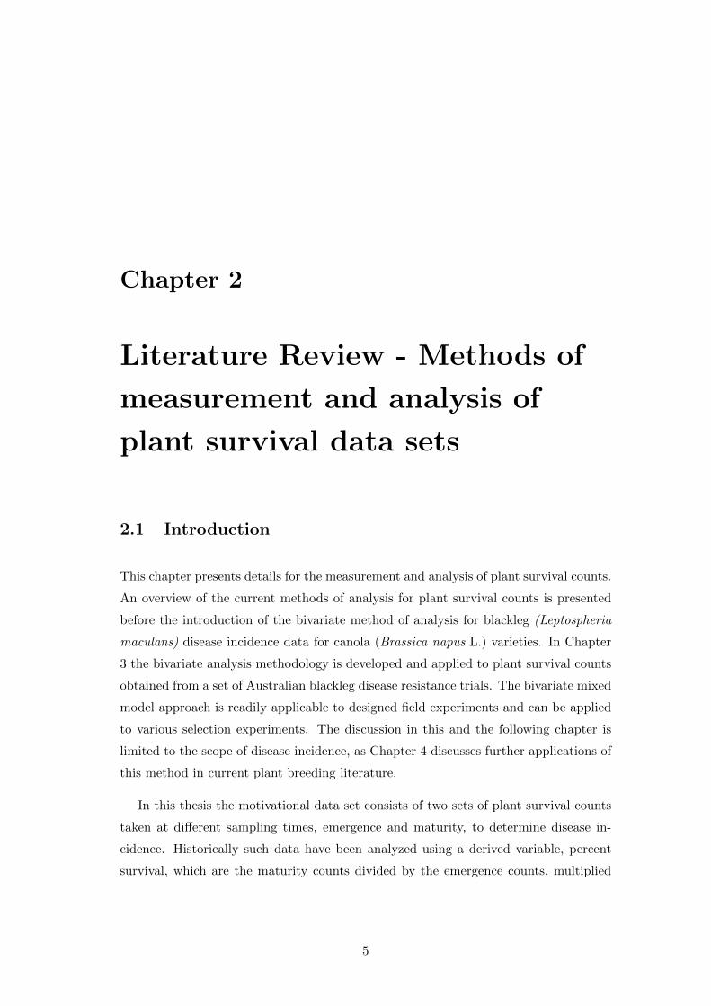
ditions. Canola is predominantly grown across southern Australia (Fig. 1.1), from the
sand-plain agriculture with winter dominated rainfall conditions in Western Australia
to the clay loamy soils of Eastern Australia which are characterized by equi-seasonal
rainfall (Kirkegaard et al., 2011). Such growing environments have been previously
reported as extremely variable between locations as well as between seasons (Chapman
et al., 2003).
Figure 1.1: Canola production regions across southern Australia - Shaded areasindicate potential geographic regions where canola is grown across Australia. This diagramis reproduced from ABS (2008).
2

The principal objectives of a plant breeding program are to select new combinations
of genotypes/entries for such target population of environments (Comstock et al., 1996),
for release as new commercial varieties and also as parents for the next cycle of breeding
and selection. Selection is based on measurements on variety plots from designed trials
across multiple locations, termed Multi-environment trial(s) (METs). The standard
for selection in these programs is based on Best Linear Unbiased Predictions (BLUPs)
of variety effects from mixed model analysis (Bauer et al., 2009, Piepho et al., 2008).
Such trials and analysis methods not only enable an estimate of genetic value, but
also breeding value when pedigree (ancestry) information is included (Oakey et al.,
2006, 2007). Note that here and in other parts of the thesis genetic value refers to
the total genetic effect of an individual which is composed of component additive and
non-additive genetic effects, and breeding value refers to the additive component only
and represents the ability of an individual to pass on their alleles to their progeny
(Bauer et al., 2009). The inclusion of pedigree information in mixed model analysis is
an attempt to model the gene to phenotype relationship previously reviewed by Cooper
et al. (2005).
A brief introduction is only provided here, as there are two literature reviews in this
thesis, which provide an in depth discussion on the literature concerning components
of research: correlated traits, ancestry (pedigree information) and environments.
The first half of the thesis focuses on correlated traits. While selection is usually
undertaken on several traits within a breeding program, plant breeding programs rarely
use multivariate methods which are common place in animal breeding programs (Com-
stock et al., 1996, Piepho et al., 2008). Selection on multiple traits avoids any bias
in selection especially when traits are highly correlated (Lin et al., 1985). Using the
motivational data set comprising plant survival data from the National Blackleg trials
across Australia, Chapter 2 provides a literature review on the analysis and measure-
ment of plant survival data. Following on from this, Chapter 3 describes and applies
a bivariate mixed model approach for the analysis of plant survival data. Chapter 4
presents a literature review, extending the applications of the bivariate mixed model
approach to other plant breeding selection experiments.
The promotion of new cultivars in a breeding program is based on a large set of
3

1. INTRODUCTION
potential genotypes tested across a set of target environments, so the estimation of
genetic value is the core of a breeding program (Piepho et al., 2008). The inclusion
of pedigree information by Oakey et al. (2007) in mixed model analysis of MET data
has resulted in plant breeding programs increasingly using breeding values for parental
selection (Atkin et al., 2009, Beeck et al., 2010, Crossa et al., 2006, Cullis et al., 2010,
Kelly et al., 2009). A literature review on the inclusion of pedigree information in plant
breeding trials is covered in Chapter 5. This is followed in Chapter 6 by the presentation
of a background review of the motivating data set of the second half of the thesis, an
actual plant breeding program data set kindly provided by Canola Breeders Western
Australia Pty Ltd, coded for anonymity.
In the second half of the thesis, Chapter 7 focuses on another method of improving
gain from selection, that is, through the control of environmental effects using spatial
analysis within the mixed model framework. Data from field trials exhibit spatial
variation, which arises from the physical location of plots within a field (Smith et al.,
2002b). If not accounted for, the presence of extraneous variation can complicate the
analysis, as well as reduce the efficiency of selection (Stefanova et al., 2009). This
is first addressed through observing the inclusion of ancestry (pedigree) information
in mixed models in Chapter 7. Chapter 8 then uses these spatial models within a
MET framework to observe how environment impacts on entry performance (genotype
by environment interaction) of entry types (hybrid and non-hybrid) within a breeding
program. The last chapter covers a topic of interest that arose during research, which is
a potential barrier to adoption of mixed model analysis with pedigree information - the
extensive time to analysis completion. While this thesis focuses canola, the outcomes
of this research has implications for all plant breeding programs whether hybrid or
self-pollinated crops.
4
Chapter 2
Literature Review - Methods of
measurement and analysis of
plant survival data sets
2.1 Introduction
This chapter presents details for the measurement and analysis of plant survival counts.
An overview of the current methods of analysis for plant survival counts is presented
before the introduction of the bivariate method of analysis for blackleg (Leptospheria
maculans) disease incidence data for canola (Brassica napus L.) varieties. In Chapter
3 the bivariate analysis methodology is developed and applied to plant survival counts
obtained from a set of Australian blackleg disease resistance trials. The bivariate mixed
model approach is readily applicable to designed field experiments and can be applied
to various selection experiments. The discussion in this and the following chapter is
limited to the scope of disease incidence, as Chapter 4 discusses further applications of
this method in current plant breeding literature.
In this thesis the motivational data set consists of two sets of plant survival counts
taken at different sampling times, emergence and maturity, to determine disease in-
cidence. Historically such data have been analyzed using a derived variable, percent
survival, which are the maturity counts divided by the emergence counts, multiplied
5

2. LITERATURE REVIEW - METHODS OF MEASUREMENT ANDANALYSIS OF PLANT SURVIVAL DATA SETS
by a hundred. This chapter instead explores the analysis of such data using a bivariate
framework of analysis, arguing that each trait (that is, counts at emergence and at
maturity) has different biological, environmental and genetic factors and thus should
be treated as individual traits. This chapter commences with a description of measures
of disease in plant breeding experiments and is followed by a discussion of the bivariate
analysis in the context of the blackleg disease resistance data set in terms of biological
and statistical arguments.
2.2 Measures of disease
Plant disease infection can range from mild symptoms to large scale crop destruction.
Biologically, the main method of plant pathogen control is the breeding of host plant
resistance (Waller et al., 2002). Accurate measures of disease are critical not only
for the identification of disease, but also for selection against disease resistance in the
field (Rempel and Hall, 1996). There are numerous methods of measuring disease, a
common method is disease incidence, defined as the number of plants infected out of the
total number of plants assessed (Parlevliet, 1979). In some cases, measures of disease
incidence can be taken across time, resulting in multiple observations (Parlevliet, 1979).
This is the case with the measurement of blackleg disease of canola in Australia, where
incidence is measured in terms of counting the number of seedlings that have emerged
and then recounting the number of plants present at maturity. These data have been
used to compute a derived variable, percentage survival of established plants, which
is analyzed as the trait of interest. These measures are undertaken in designed field
trials across Australia (Li et al., 2008, Marcroft et al., 2012) and in France (Pilet et al.,
1998). In the proposed study however, the analysis of blackleg disease incidence is
considered within a bivariate framework where the plant survival counts are treated as
two separate traits.
2.3 Blackleg disease incidence
Blackleg is a fungal disease of Brassica napus (rapeseed or canola) (Punithalingam
and Holliday, 1972), which causes severe yield losses in Australia and worldwide (Fitt
6

2.3 Blackleg disease incidence
et al., 2006, West et al., 2001). Grain yield losses associated with blackleg have been
reported to range from less than 10% to greater than 50% (Hall, 1992, West et al.,
2001, Zhou, 1999). Blackleg disease is of special interest in Australian agriculture, as it
destroyed most rapeseed crops soon after their introduction to Australia in the 1960’s
and 1970’s (Gugel and Petrie, 1992, Khangura and Barbetti, 2001) and discouraged
further attempts to grow the crop for several years. The industry however recovered,
stimulated primarily by the release of canola varieties in 1993 with increasing levels of
resistance to blackleg (Khangura and Barbetti, 2001). Since then, the acreage planted
to canola has increased dramatically due to crop profitability (ABARES, 2011), and
agronomic benefits associated with canola in crop rotations, which include the control
of cereal root diseases and flexibility in weed management (Kirkegaard and Sarwar,
1999, Turner, 2004). However, blackleg disease remains an ongoing threat to Australian
canola production due to favorable conditions for epidemics in Australian environments.
Figure 2.1: The lifecycle of blackleg disease - Reproduced from Howlett et al. (2001).
The lifecycle of L. maculans comprises a single sexual generation of ascospores and
multiple asexual generations of pycnidiospores (Hayden et al., 2007). Ascospores, the
7

2. LITERATURE REVIEW - METHODS OF MEASUREMENT ANDANALYSIS OF PLANT SURVIVAL DATA SETS
primary inoculum, are discharged from pseudothecia formed on stubble remnants, on
which the fungus survives over the summer period in Australia (Gladders and Musa,
1980, Hall, 1992, McGee and Emmett, 1977, West et al., 2001). Ascospore release
occurs after rain events (McGee and Emmett, 1977). Hence, in Australian agricul-
tural systems seedling establishment and ascospore release coincide, providing ideal
conditions for severe crown canker epidemics (Barbetti and Khangura, 1999). Seedling
infection occurs when the fungus enters the cotyledons through stomata or wounds in
which the hyphae extend (Hammond and Lewis, 1987, Hayden et al., 2007, Howlett
et al., 2001). The fungus then grows internally from leaf infections through petiole and
stem tissue to the crown of the plant, where it causes cell necrosis and the girdling
of the stem. The crown rot is accompanied by black or purple staining of the stems,
which is characteristic of the disease (Howlett et al., 2001).
To date, the main method of controlling blackleg disease is through breeding for im-
proved cultivar resistance (Kirkegaard et al., 2006, Rimmer and Van den Berg, 1992).
This is confirmed on a national scale in Australia by the annual testing and publication
of the National Blackleg Resistance ratings for commercial canola varieties. These resis-
tance ratings are determined by measuring disease incidence from designed field trials
at multiple locations across southern Australia, coordinated by the National Blackleg
Group (NBG) with individual trials managed by public researchers and private plant
breeding companies. The importance of these disease ratings to farmers is reflected by
the recent publication of the resistance ratings on the National Variety Trial (NVT)
data base (http://www.nvtonline.com.au/home.htm).
While there are numerous methods for quantifying blackleg disease infection, see
Rimmer and Van den Berg (1992) for full listing, the rating of designed field experiments
necessitates the use of a measure that is not only quick, but also relatively easy and
accurate to undertake. Plant survival counts, which compares counts at emergence
and maturity, are relatively easy to measure on large scale field trials. Further such a
measure reflects the economic losses associated with blackleg disease (Fitt et al., 2006).
Plant survival counts have been successfully used for measuring disease resistance in
many Australian plant breeding programs for the past 30 years (Marcroft et al., 2002).
As a result, the annual National Blackleg Resistance ratings, published by Canola
Association of Australia (http://www.australianoilseeds.com) and some researchers use
8
2.4 Bivariate analysis
this method as a measure of disease incidence (Li et al., 2008, Marcroft et al., 2002,
2012).
The studies that have used plant survival counts as a measure of blackleg disease
incidence, (Li et al., 2008, Marcroft et al., 2002, 2012), all use a univariate analysis of
the percent survival values within an analysis of variance (ANOVA) framework. The
only other study in blackleg disease to use a variation of this disease incidence measure,
percentage of plants infected per plot, is the study by Rempel and Hall (1996). In this
case, they also used a univariate analysis of percent infected plants, however this was
within a repeated measures ANOVA framework.
Traditionally, the NBG have analyzed ‘percent survival’ values, which are calculated
by dividing maturity counts by emergence counts and multiplying this by a hundred.
This derived variable is then subjected to a univariate analysis using the spatial mixed
model approach of Gilmour et al. (1997). This enables a single site analysis of each of
the disease nursery trials to determine spatial models for errors as well as to diagnose
and remove outliers. These single sites are then combined across sites in a second stage
of analysis, known as a Multi Environment Trial (MET) and analyzed using a factor
Analytic (FA) variance structure of (Smith et al., 2002b). The MET analysis enables
an individual genetic variance for each site and a genetic covariance between pairs of
sites (Smith et al., 2001b). To distinguish this analysis from the proposed bivariate
approach, the univariate analysis will be referred to as the ‘historical analysis’. This
chapter proposes the use of a bivariate method of analysis where the two analyzed
‘traits’ are the plant survival counts at emergence and at maturity.
2.4 Bivariate analysis
2.4.1 Biological motivations
The main motivation for a bivariate analysis of plant survival data is that each sam-
pling time, emergence and maturity, constitutes an individual ‘trait’, and each may
be effected by different biological, genetic and environmental factors. Hence it would
not only be statistically but also biologically more accurate to determine trait specific
spatial models, outlier detection and error and genetic variance. This section discusses
9
2. LITERATURE REVIEW - METHODS OF MEASUREMENT ANDANALYSIS OF PLANT SURVIVAL DATA SETS
the biological reasons for using a bivariate framework for the analysis of plant survival
data for blackleg disease.
There are two types of varietal resistance to blackleg disease, quantitative (poly-
genic) and qualitative (major gene) (Leflon et al., 2007). Quantitative resistance is
evaluated in adult plants in field nurseries and results in the reduced severity of disease
symptoms, however it is known to be partial, and can succumb under high disease pres-
sure resulting in significant yield losses (Khangura and Barbetti, 2001, Sivasithamparam
et al., 2005). Further, quantitative resistance is also known to be strongly affected by
environmental conditions (Balesdent et al., 2001, Delourme et al., 2008, Fitt et al.,
2006). Qualitative resistance however, is controlled by major genes, and can provide
complete resistance to disease symptoms and infection (Ansan Melayah et al., 1997).
This is race-specific resistance, that is, provides resistance against races of blackleg and
as a result exerts a higher selection pressure on the blackleg population.
In addition to variation in the type of varietal resistance, studies have also shown
that these types of resistance are different based on the stage of plant growth (Ballinger
and Salisbury, 1996, Rempel and Hall, 1996, Roy, 1984). Ballinger and Salisbury (1996)
demonstrated that there is a differential response in seedling and mature plant resis-
tance to blackleg and in some cases resistance improves with age. This was recognized
by the above study of Rempel and Hall (1996) who attempted to observe the differential
biological factors associated with the sampling time in field evaluation trials for black-
leg disease using a repeated measures ANOVA framework. Bivariate analysis allows for
changes in genetic variance across sampling times and this could provide insight into
the different mechanisms of disease resistance present at the particular plant growth
stage.
The epidemiology of blackleg also differs at the two sampling times. The focus of
attention on blackleg infection is usually at the mature plant stage, as this is when
economic losses occur due to reduced seed production. However, studies have also
demonstrated that blackleg infection at the seedling stage can result from soil borne
ascospores and pycnidiospores (Li et al., 2007, Sosnowski et al., 2006). The study by
Li et al. (2007), found that infection at the seedling stage can result in seedling death.
10
2.4 Bivariate analysis
A bivariate analysis of the two plant counts may provide insight into the differential
impact of blackleg disease at the different sampling times.
In addition to the above, counts at emergence are also affected by different environ-
mental and biological factors that arise at seedling emergence, which could be caused
by seed source differences. Seedling emergence is a factor that cannot be controlled
in disease nurseries, as it is affected by soil fertility, salinity, compaction, tillage and
surface residues (Forcella et al., 2000). Seed source differences on the other hand arise
in seed lot variations, from factors such as age of seed (Finch Savage, 1986), the storage
environment of the seed (Ellis and Roberts, 1980), and seed production environment
(Ellis et al., 1993). While variation in seed source is a known issue across Australian
blackleg disease nurseries, these issues have been confounded in the past with disease
effects in the derived variable, percentage survival.
Thus there are biological, genetic and environmental differences between the two
sampling times and this necessitates the treatment of them as individual traits. The
bivariate analysis is able to accommodate this, hence it will enable a discussion on such
sampling time factors, unlike the historical analysis in which such effects are masked.
2.4.2 Statistical motivations
Statistically, the bivariate approach is preferred as it allows for (i) the modeling of
error, such as spatial field trend for each trait (ii) the identification of outliers for each
trait and (iii) the examination of individual trait genetic effects. For points one and
two, these may be masked when using the derived variable of the historical approach.
With the third point, an examination of the genetic effects for each trait may reveal
greater insight into plant pathogen interactions.
The modeling of spatial trend for each trait is a valuable component of a bivariate
framework. Previous studies have demonstrated that improved estimates of treat-
ments effects are obtained after correcting for environmental effects in designed field
experiments, for both agriculture or forestry experiments (Dutkowski et al., 2006). In
agricultural field trials this is achieved through the use of spatial analysis (Cullis et al.,
1998, 2006, Gilmour et al., 1997). Until recently, spatial analysis has mainly focused on
11

2. LITERATURE REVIEW - METHODS OF MEASUREMENT ANDANALYSIS OF PLANT SURVIVAL DATA SETS
annual crops or forestry trials where only one measure is taken on a plant (de Resende
et al., 2006). Other than the study by de Resende et al. (2006) there are very few
examples of studies which evaluate the impact of spatial analysis on repeated measures
or multivariate data.
A forestry based study by Dutkowski et al. (2006) indicated that spatial analysis
improved genetic response predictions by more than 10% for 20 out of the 216 traits,
tested. Most importantly this study demonstrated that some traits (growth) responded
better to spatial analysis than others (fungus damage) resulting in significant model
improvement. Dutkowski et al. (2006) also showed that many measures of model fit,
such as in error variance, prediction accuracy and standard error of genetic variance
estimates improved from the modelling of individual trait spatial error. This study
demonstrated that spatial analysis can lead to modest to large improvements in selec-
tion. In the blackleg data set the plant counts are taken on the same plot, however the
type of error at each sampling time could possibly reflect a different spatial modelling
for each trait, as they are known to be affected by different environmental, biological
and genetic components.
The measurement of plant counts at two sampling times on the same variety plot
is essentially a form of a repeated measures experiment. An important feature of
repeated measures experiments is that the measures on the same experimental unit
or sequence of measures in time are likely to be correlated (Gurevitch and Jr, 1986,
Littell et al., 1998). Hence it is important to model such variance covariance structure
in mixed model analysis (Littell et al., 1998, Piepho and Mohring, 2006). Under the
historical analysis this was ignored by using a derived variable, which does not require
the modeling of this covariance. Given that the aim of testing entries in the blackleg
disease nurseries is to accurately determine disease resistance ratings of commercial
canola varieties, a bivariate mixed model methodology enables such data to be more
accurately modeled.
Further, the variances of the repeated measures may often change with time (Littell
et al., 1998), which was demonstrated to be the case in blackleg by the study of Rempel
and Hall (1996). Of particular interest is the variance attributed to each sampling time
as it may be a reflection of the different genetic, biological and environmental impact
12

2.5 Summary
of the disease. As a result it will be an important component of the bivariate analysis
to be able to model the individual variances and covariance between sampling times.
Selection is improved when based on multiple traits, so that any bias in selection
due to correlated traits is avoided (Kerr, 1998). Even slight improvements of accuracy
can result in large economic effects in large populations (Pollak et al., 1984), which is
often what is encountered in breeding programs. As a result, multi-trait analyses are
commonly utilized in animal breeding programs, (Henderson and Quaas, 1976, Mrode
and Thompson, 2005) yet there are very few plant breeding programs in annual crops
that utilize this (Piepho et al., 2008).
Theoretically, multivariate methods can result in increases in the accuracy of eval-
uations as it utilizes information from phenotypic and genotypic correlations between
traits (Mrode and Thompson, 2005). In addition, the studies by Thompson and Meyer
(1986) and Villanueva et al. (1993) have shown that a bivariate analysis can result in
gains in accuracy in evaluation for a trait when using other correlated traits. Further,
multivariate analysis would eliminate any potential bias that occurs from the selection
of a correlated trait (Pollak et al., 1984, Kerr, 1998), that is, any bias in the evalua-
tion that arises due to disregarding covariance structures between traits is avoided (Lin
et al., 1985).
2.5 Summary
Plant survival data are often composed of multiple measures used to form a derived
variable such as percent survival values. These derived values are then subject to a uni-
variate analysis. Chapter 3 will develop and apply a bivariate mixed model approach
where the multiple measures are realized as individual traits. This is demonstrated us-
ing the motivational example of a set of designed field trials of blackleg disease incidence
data from the Australian National Blackleg Resistance trials. This literature review
has discussed how such counts can be subject to different biological, environmental
and genetic factors, and the bivariate framework can be statistically more accurate in
accommodating this with trait based spatial modeling, outlier detection and genetic
variance.
13

2. LITERATURE REVIEW - METHODS OF MEASUREMENT ANDANALYSIS OF PLANT SURVIVAL DATA SETS
14

Chapter 3
A bivariate mixed model
approach for the analysis of plant
survival data
The motivating data set for this chapter consists of a series of blackleg disease nurs-
ery trials, kindly provided by the National Blackleg Group (NBG). These trials are
used to determine the annual disease resistance ratings for canola varieties and are co-
ordinated by the NBG and published annually by the Canola Association of Australia.
The NBG is responsible for deciding the published blackleg rating for each entry, which
by convention is based on an analysis of the previous three years of blackleg plant sur-
vival data (square root percentage survival) under high disease pressure. This chapter
presents a bivariate mixed model methodology for the analysis of such a plant survival
data set. The chapter commences with an overview of the current protocol for the run-
ning of the National Blackleg Disease nurseries and the measurement of plant disease
is presented. This is then followed by a section on the description of the mixed model
approaches (univariate and then bivariate) each followed by an example using the York
disease nursery site and summarized for the other disease nursery sites. This chapter
concludes with a discussion on the bivariate mixed model approach. The methodology
and analysis presented in this chapter has been published in the journal Euphytica,
and a reprint of this submission is attached in the Appendices (Appendix A).
15

3. A BIVARIATE MIXED MODEL APPROACH FOR THE ANALYSISOF PLANT SURVIVAL DATA
3.1 Data set description
The data comprises 140 commercial and unreleased entries (varieties) of B. napus from
the 2009 growing season disease nurseries. These disease nurseries were located at 6
sites across southern Australia in canola producing areas of medium to high rainfall
(Table 3.1 and Fig. 3.1). Disease nursery sites were managed and run by public
researchers and private breeding companies. The sites were composed of designed
experiments with varieties from all the herbicide groups, i.e. conventional, Clearfield R©
and Triazine Tolerant (Table 3.1). In this data set all the trials were designed as
randomized complete block designs, sometimes with extra replicates of control entries.
All experiments were laid out as a rectangular array indexed by rows and columns
(Table 3.2). The design and implementation of these trials were left up to the discretion
of the breeding companies or research groups managing them. However the NBG
coordinated trial management and ensured quality assurance through the use of unified
protocols, see Marcroft (2009) for a full listing of disease nursery protocols. High disease
levels at all nurseries were maintained by growing entries alongside or on disease stubble
obtained from the previous season.
Bakers Hill●
Clear Lake●
Shenton Park●
Wagga Wagga●
Wonwondah●
York●
Figure 3.1: Location of blackleg disease nurseries across Australia - Geographiclocations of the six blackleg (Leptospheria maculans) disease nurseries across southernAustralia during the 2009 growing season.
16

3.2 Measuring disease incidence
Table 3.1: Location based trial details: state, stubble type, entry herbicide type andaverage plant counts at emergence (eme) and maturity (mat) for each of the 2009 blacklegdisease nurseries.
Location State Stubble Type Herbicide Type? AverageEme Mat
Bakers Hill WA Bravo TT C, Cl, TT 60 35Clear Lake VIC 45Y77 C, Cl, TT 50 33Shenton Park WA CB Telfer C, Cl, TT 75 57Wagga Wagga NSW Bravo TT C, Cl, TT 34 10Wonwondah VIC AV-Garnet C, TT 37 14York WA ATR-Cobbler C, TT 59 13
?Herbicide type acronyms: C=Conventional, Cl=ClearfieldR© and TT=Triazine Tolerant
Table 3.2: Details of blackleg disease nursery experiments during the 2009 growing season.The number of entries, columns, rows and blocks are listed for each experiment in this dataset.
Location Location Code Entries Columns Rows Blocks?
Bakers Hill BH 57 3 57 3Clear Lake CL 18 4 20 4Shenton Park SP 65 22 9 4Wagga Wagga WA 74 15 16 3Wonwondah WO 31 12 10 3York YK 78 3 79 3
?Note that “Blocks” correspond to biological replicates.
3.2 Measuring disease incidence
Plots of entries were sown with a targeted minimum of 100 seedlings per plot. Plant
counts were first taken at emergence, which corresponds to the open cotyledon stage of
plant growth and occurs approximately 4− 6 weeks after plant emergence. Plants are
then recounted at maturity that is the windrowing stage. Disease nursery sites were
only included in the analysis if there was less than 30% survival on susceptible control
entries. Historically, plots with less than 20% emergence were deemed unreliable and
defined as missing, however for this analysis the data from these missing plots were
obtained from trial managers and included in the data set.
17

3. A BIVARIATE MIXED MODEL APPROACH FOR THE ANALYSISOF PLANT SURVIVAL DATA
3.3 Univariate analysis
The count data were first log-transformed before analysis. This ensured that the resid-
uals approximated a Gaussian distribution with a constant variance. This has been
historically appropriate for this data set and also ensures that the predicted counts are
non-negative, which is of biological significance to this analysis.
The component traits of the bivariate analysis, plant survival counts at emergence
and maturity, were first each subjected to a univariate analysis to enable appropriate
spatial model selection using the approach of Gilmour et al. (1997). Field experiments
often have spatial variation due to the physical location of individual plots in the
field. The approach of Gilmour et al. (1997) enables modeling of spatial trend for field
trials, which accounts for three sources of variation namely global, local and extraneous
variation. Global trend refers to variation that occurs across the field, local represents
short-term trend such as soil fertility and extraneous variation is often the result of
experimental procedures that are aligned with rows and columns (Gilmour et al., 1997).
Local trend is accommodated within the mixed model by an appropriate covariance
structure of which the separable autoregressive process of order 1 (denoted AR1×AR1)
is the most commonly used (Gilmour et al., 1997). Models for non-genetic variation
encompass model terms for both experimental design and spatial variation.
3.3.1 Statistical model
Each disease nursery is comprised of a rectangular array of plots with r rows and c
columns, so that the number of plots in an experiment is given by n = rc. Additionally,
m is the number of entries and b is the number of blocks in the experiment.
The base-line spatial mixed model for the (log transformed) plant survival counts for
each sample time (j = 1, 2), with j corresponding to 1 at emergence and 2 for maturity
can be written as,
yj = Xτ j +Zvuvj +Zbubj + ej (3.1)
; yj is a n×1 vector of plant survival counts for individual plots within an experiment,
ordered as rows within columns; X, Zv and Zb are design matrices for fixed effects,
18

3.3 Univariate analysis
random entry effects and random block effects respectively; τ j is the vector of fixed
effects; uvj is the m×1 vector of random entry effects; ubj is the b×1 vector of random
block effects and ej is the vector of residuals ordered as per the data vector. There are
no sub-scripts associated with the design matrices since, for the base-line model, they
are the same for both sampling times.
The assumptions for the univariate base line model (Equation 3.1) are,
E(yj) = Xτ j
E(uvj) = E(ej) = 0
The variance assumptions for the entry effects in Equation 3.1 are:
var(uvj
)= σ2
vjIm
where σ2vj is the entry variance at sampling time j and Im is an identity matrix of
order m.
For block effects, the variance assumptions are:
var(ubj
)= σ2
bjIb
where σ2bj is the block variance at sampling time j and Ib is an identity matrix of order
b.
The variance matrix for the errors (Rj) assuming a separable AR1 process is:
var (ej) = Rj = σ2jΣcj ⊗Σrj
where σ2j is the error variance at sampling time j, and Σcj and Σrj are correlation
matrices of dimensions c×c and r×r for columns and rows respectively of AR1 processes
in the column and row directions. Each matrix is a function of a single autocorrelation
parameter ρcj and ρrj for the column and row dimensions respectively. Note that in
some experiments where there were four or less columns, it was assumed that there was
independence for errors in the column dimension, so that Σcj=Ic.
The var(yj)
is then,
var(yj)
= σ2vjZvZv
T + σ2bjZbZb
T +Rj
19
3. A BIVARIATE MIXED MODEL APPROACH FOR THE ANALYSISOF PLANT SURVIVAL DATA
3.3.2 Checking the adequacy of the spatial model
Following the univariate analysis, an examination of the adequacy of the spatial models
was undertaken. This involved using two diagnostics, a 3D sample variogram and a plot
of residuals against row/column numbers (termed as residual plots) from Gilmour et al.
(1997). Residual plots are used to observe for local trend and possible outliers. The
sample variogram, enables for the visualization of extraneous variation/global trend as
well as to check the adequacy of the variance structure for local trend. If additional
terms were needed to accommodate any observed extraneous variation, they were added
to the initial base mixed model. For example, τ j would include additional terms for
linear regression across rows, or additional random effects terms would be added to the
base-line model.
While the residual plot is used to visualize possible outliers, the Alternative Outlier
Mixed Model (AOMM) in ASReml-R (Smith et al. unpublished), was used to pro-
duce Studentised conditional residuals as part of the outlier identification diagnostics.
Studentised conditional residual values greater than 3.5 where identified as outliers,
however the plant breeder was still consulted to confirm these.
3.3.3 Estimation and Fitting
The fitting of mixed models involves two processes, firstly the variance parameters
(σ2vj ,σ
2bj , ρcj , ρrj and σ2
j ) are estimated using the REML method of Patterson and
Thompson (1971) and secondly these estimates are then used to solve the mixed model
equations (Henderson, 1975) (Equation 3.2). This results in (empirical) Best Linear
Unbiased Estimates of fixed effects (E-BLUEs), and (empirical) Best Linear Unbiased
Predictions of the random effects (E-BLUPs). The term ‘empirical’ is used as the
variance parameters are unknown and are estimated form the data.
20

3.3 Univariate analysis
The mixed model equations for the base line univariate model (Equation 3.1) are, XTR−1j X XTR−1
j Zv XTR−1j Zb
ZvTR−1
j X (ZvTR−1
j Zv + (σ2vj)
−1Im) ZvTR−1
j Zb
ZbTR−1
j X ZbTR−1
j Zv (ZbTR−1
j Zb + (σ2bjIb)
−1)
τ j
uvj
ubj
(3.2)
=
XTR−1j yj
ZvTR−1
j yj
ZbTR−1
j yj
where τ j is the E-BLUE of the fixed effects and uvj and ubj are the E-BLUPs of
the random effects for entries and blocks respectively.
All models in this chapter and the thesis were fitted in the software package ASReml-
R (Butler et al., 2009).
3.3.4 Univariate analysis results
3.3.4.1 York disease nursery
The univariate analysis is described in detail for the disease nursery at York. The York
disease nursery had n = 237 plots, with r = 79 rows and c = 3 columns, b = 3 blocks
and m = 78 entries, see Table 3.2. There should be 79 entries, however due to lack of
seed for one of the entries, an extra plot of another entry was sown. The initial base
line model, equation 3.1 was fitted, with independence assumed in the column direction
for the spatial model, so that var (ej) = Rj = σ2j I ⊗Σrj .
First the emergence model is considered. The resulting plot of residuals and the
sample variogram can be seen in Fig. (3.2). The residual plot indicated the presence
of three outliers. These were confirmed by checking AOMM statistics, which indicated
unusually large studentised conditional residuals. These were omitted from the analysis
by setting the plots to the missing value qualifier. In addition, the sample variogram
indicated the presence of extraneous variation in the row direction, observed by the
up/down pattern. This was accommodated by fitting random row effects in the model.
Having removed the outliers and included a term for random row effects, the model for
21
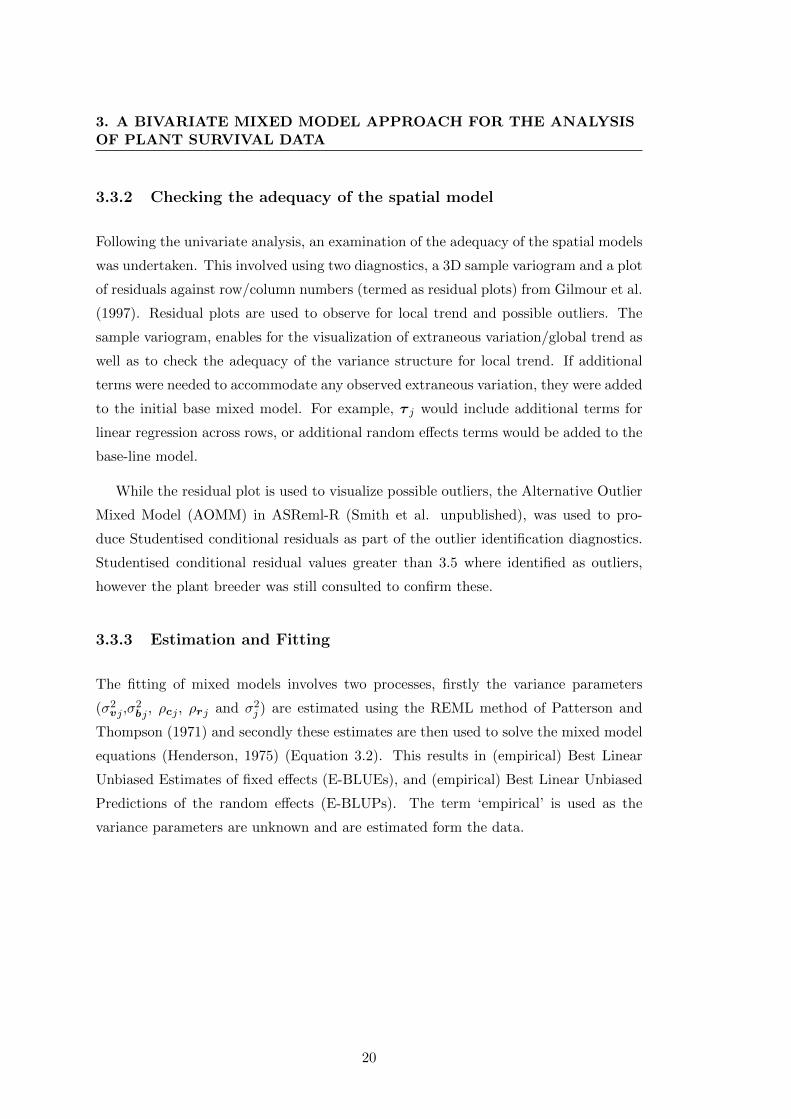
3. A BIVARIATE MIXED MODEL APPROACH FOR THE ANALYSISOF PLANT SURVIVAL DATA
emergence was then refitted,
y1 = X1τ 1 +Zv1uv1 +Zb1ub1 +Zr1ur1 + e1 (3.3)
where the dimensions of the respective matrices are as follows, y is a 237×1 data vector;
τ is the grand mean with corresponding design matrix X with dimensions 237× 1; uv
is a 78 × 1 vector of random entry effects with corresponding design matrix Zv of
dimensions 237 × 78; ub is a 3 × 1 vector of random block effects with corresponding
design matrix Zb of dimensions 237 × 3; ur is a 79 × 1 vector of random row effects
with corresponding design matrix Zr of dimensions 237× 79; and lastly, e is a 237× 1
vector of residuals
The resulting REML estimates of variance parameters for this equation are:
σv21 = 0.4
σb21 = 0.04
σ12 = 0.382
ρr1 = 0.72
The re-fitting of Equation 3.3 resulted in the sample variogram in Fig. 3.3, which
indicated a more adequate spatial model.
In terms of REML estimates, the genetic variance component was non-zero for emer-
gence (0.400), however the block variance component was almost zero at 0.041. The
row autocorrelation value was large at 0.72 indicating strong smooth spatial variation.
The error variance for the emergence mixed model was 0.382.
Now consider the maturity model at this nursery site. There appeared to be no
extraneous variation, and only a single outlier was detected and set to a missing value.
Similar to the emergence mixed model, the REML estimate of the genetic variance
component was non-zero for maturity. The entry variance estimate was larger for
maturity (0.511) than for emergence (0.400) (Table 3.5). The block variance component
were almost zero 0.066 for maturity as well. The error variance for the maturity model,
was smaller than that of emergence model (Table 3.4) and the autocorrelation for trend
in the row direction was much stronger for emergence (0.72) than maturity (0.22) (Table
3.3) .
22

3.3 Univariate analysis
Figure 3.2: York disease nursery initial plot of residuals and sample variogram- Initial plot of residuals and sample variogram from the univariate emergence model atthe York disease nursery.
23

3. A BIVARIATE MIXED MODEL APPROACH FOR THE ANALYSISOF PLANT SURVIVAL DATA
Figure 3.3: York disease nursery final plot of residuals and sample variogram -Plot of residuals and sample variogram from the univariate emergence model at the Yorkdisease nursery after the addition of random row effects and removal of outliers.
24

3.3 Univariate analysis
3.3.4.2 All disease nurseries
For each trial and sampling time, the base line univariate model was fitted (Equation
3.1). Non-stationary trend and extraneous variation components were needed for 5
out of 6 disease nursery sites. None of these sites had the same extraneous variation
components for both traits (Table 3.3). Overall there were more extraneous variation
terms included for the emergence model than the maturity mixed model. Stationary
trend differed between the trait models, for column and row AR1 values (Table 3.3).
There were two instances (Shenton Park and Wonwondah) where spatial correlation was
modeled for the column dimension as well as the row dimension. For these two disease
nurseries, the AR1 values for each dimension differed largely for each trait (Table 3.3).
The row AR1 values ranged from −0.13 to 0.72 for the emergence model and −0.07
to 0.28 for the maturity models. The greatest difference between traits for row AR1
values was for the York and Clearlake disease nurseries (Table 3.3). Further, at 4 out
of the 6 disease nurseries these row AR1 values were larger for the maturity model than
the emergence model. Overall the largest AR1 value was observed for the emergence
trait at York (0.72) and the maturity trait at Wagga (0.28). Additionally, the outliers
removed from the analysis differed for each trait across disease nurseries with only one
disease nursery having the same number of outliers removed for each trait (Table 3.3).
REML estimates of entry variance components across all disease nursery sites were
non-zero, ranging from 0.033 at Wonwondah to 0.400 at York for the emergence models
and 0.127 at Bakers Hill to 0.768 at Wagga Wagga for the maturity models (Table 3.5).
Thus there was entry variation observed for each trait at all disease nursery locations.
Additionally, the entry variance components for maturity were always substantially
larger than those of emergence, except for Bakers Hill where the variance components
appeared similar at 0.108 and 0.127 for the emergence and maturity models respectively.
Across all disease nurseries except Wonwondah, REML estimates of error variance
components were larger for the maturity trait than the emergence model (Table 3.4).
For the emergence models these ranged from 0.015 at Shenton Park to 0.382 at York.
For the maturity models these ranged from 0.031 at Wonwondah to 0.317 at Bakers
Hill (Table 3.4). REML estimates of block variances at all disease nurseries however,
appeared close to 0 (Table 3.3).
25
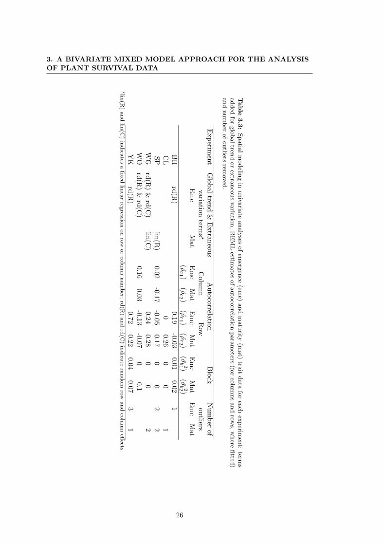
3. A BIVARIATE MIXED MODEL APPROACH FOR THE ANALYSISOF PLANT SURVIVAL DATA
Tab
le3.3
:S
patial
mod
eling
inu
nivariate
analy
sesof
emerg
ence
(eme)
an
dm
atu
rity(m
at)trait
data
foreach
exp
erimen
t:term
sad
ded
forglob
al
trend
or
extran
eou
sva
riation
,R
EM
Lestim
ates
of
au
toco
rrelatio
np
arameters
(forcolu
mn
san
drow
s,w
here
fitted
)an
dnu
mb
erof
ou
tliersrem
oved.
Exp
erimen
tG
lob
al
trend
&E
xtran
eous
Au
tocorrelation
Blo
ckN
um
ber
ofvariation
terms?
Colu
mn
Row
outliers
Em
eM
atE
me
Mat
Em
eM
atE
me
Mat
Em
eM
at(ρ
c1 )
(ρc2 )
(ρr1 )
(ρr2 )
(σb21 )
(σb22 )
BH
rd(R
)0.19
-0.030.01
0.021
CL
00.26
00
1S
Plin
(R)
0.02-0.17
-0.050.17
00
22
WG
rd(R
)&
rd(C
)lin
(C)
0.240.28
00
2W
Ord
(R)
&rd
(C)
0.160.03
-0.13-0.07
00.1
YK
rd(R
)0.72
0.220.04
0.073
1?lin
(R)
and
lin(C
)in
dica
tesa
fixed
linea
rreg
ression
on
rowor
colu
mn
num
ber;
rd(R
)and
rd(C
)in
dica
tera
ndom
rowand
colu
mn
effects.
26
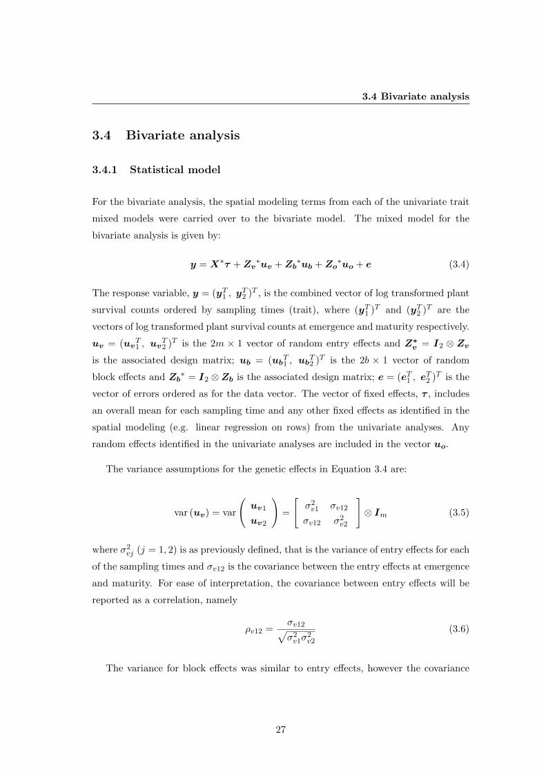
3.4 Bivariate analysis
3.4 Bivariate analysis
3.4.1 Statistical model
For the bivariate analysis, the spatial modeling terms from each of the univariate trait
mixed models were carried over to the bivariate model. The mixed model for the
bivariate analysis is given by:
y = X∗τ +Zv∗uv +Zb
∗ub +Zo∗uo + e (3.4)
The response variable, y = (yT1 , yT2 )T , is the combined vector of log transformed plant
survival counts ordered by sampling times (trait), where (yT1 )T and (yT2 )T are the
vectors of log transformed plant survival counts at emergence and maturity respectively.
uv = (uvT1 , uv
T2 )T is the 2m × 1 vector of random entry effects and Z∗
v = I2 ⊗ Zv
is the associated design matrix; ub = (ubT1 , ub
T2 )T is the 2b × 1 vector of random
block effects and Zb∗ = I2 ⊗Zb is the associated design matrix; e = (eT1 , e
T2 )T is the
vector of errors ordered as for the data vector. The vector of fixed effects, τ , includes
an overall mean for each sampling time and any other fixed effects as identified in the
spatial modeling (e.g. linear regression on rows) from the univariate analyses. Any
random effects identified in the univariate analyses are included in the vector uo.
The variance assumptions for the genetic effects in Equation 3.4 are:
var (uv) = var
(uv1
uv2
)=
[σ2v1 σv12
σv12 σ2v2
]⊗ Im (3.5)
where σ2vj (j = 1, 2) is as previously defined, that is the variance of entry effects for each
of the sampling times and σv12 is the covariance between the entry effects at emergence
and maturity. For ease of interpretation, the covariance between entry effects will be
reported as a correlation, namely
ρv12 =σv12√σ2v1σ
2v2
(3.6)
The variance for block effects was similar to entry effects, however the covariance
27

3. A BIVARIATE MIXED MODEL APPROACH FOR THE ANALYSISOF PLANT SURVIVAL DATA
was omitted between the sampling times, as the variances of blocks for both traits were
close to zero at all disease nursery sites. The variance assumptions for the vector uo
were chosen appropriately for the terms involved.
In terms of the errors a separable spatial correlation model was assumed.
var (e) = var
(e1
e2
)=
[σ2
1 σ12
σ12 σ22
]⊗Σc ⊗Σr = R (3.7)
As in the univariate analysis, σ2j (j = 1, 2) are the error variances for each of the
sampling times and σ12 is the covariance between the errors at emergence and matu-
rity. Similar to the entry covariance, the error covariance was converted to a correlation
between the traits, see Equation 3.6. The spatial correlation matrices Σc and Σr cor-
respond to autoregressive processes of order one, that is, functions of single parameters
ρc and ρr respectively. The separability assumption implies that the same spatial cor-
relation parameters are applicable for both sampling times. It may be desirable to
allow different parameters, but such models are not yet available and are the subject
of current research.
After the bivariate model was fitted E-BLUPS of entry means were obtained for
each sampling time. Note that the difference between the predicted entry means for
emergence and maturity corresponded to the percent survival scale of the historical
approach, when back-transformed. To see this, let πjk denote the predicted entry
mean for entry k at sampling time j, then
exp(π2k − π1k) =exp(π2k)
exp(π1k)(3.8)
This transformation enables entries to be assessed on the same scale as the historic
approach, percent survival. The E-BLUPs were used to produce two plots. In the
first entry means at maturity were plotted against entry means at emergence (Fig.
3.4). This plot also included a regression line of maturity against emergence, which
corresponded to the regression of the true entry effects for maturity (i.e uv2) on the
28

3.4 Bivariate analysis
true entry effects for emergence (i.e uv1). The slope is given by
β = ρv12 ×
√σ2v2
σ2v1
(3.9)
The second plot, was of the difference between E-BLUPs of entry means for emergence
and maturity plotted against the E-BLUPs of entry means at emergence (Fig. 3.5).
3.4.2 Model Comparisons
There is a potential gain in accuracy of analysis that results when using a multivariate
analysis over a univariate analysis. Prediction error variance is a measure of the gain
in accuracy that results from multiple trait analysis (Henderson, 1973, Thompson and
Meyer, 1986). The accuracy of prediction, as defined by Mrode and Thompson (2005)
is the square of the correlation between the true (uij) and predicted effects (uij) of a
variety (Equation 3.10). In the bivariate analysis of plant survival data the correlation
between true and predicted effect for entry i and sampling time j is given by,
rij = cor(uvij , uvij) =√
1− PEVvij/σ2vj (3.10)
where PEVvij is the prediction error variance, and σ2vj is the estimated genetic variance
for the sampling time (j = 1, 2). Prediction accuracies were obtained for each variety
for each disease nursery for the traits:
1. (log) emergence counts
2. (log) maturity counts
3. the difference in log counts ie. log maturity - log emergence
from three univariate analyses (ie. one for each trait) and a single bivariate analysis
(with log emergence and log maturity counts being the two variables).
To eliminate any effects of variance parameter estimation from the comparisons,
variance parameters for the univariate analyses were constrained to be the same as
those obtained from the bivariate analysis. For example, consider the disease nurs-
ery at Bakers Hill, where the REML estimates of genetic variance from the bivariate
29

3. A BIVARIATE MIXED MODEL APPROACH FOR THE ANALYSISOF PLANT SURVIVAL DATA
analysis were σv21 = 0.109 and σv
22 = 0.131 for the emergence and maturity traits re-
spectively and the estimate of the genetic correlation was ρv12 = 0.68 (Table 3.5). In
the comparable univariate analyses the genetic variances were constrained to be equal
to
1. 0.109 for the analysis of log emergence counts
2. 0.131 for the analysis of log maturity counts and
3. σv21 + σv
22 − 2ρv12σv1σv2 = 0.078 for the analysis of the differences.
Non-genetic components were constrained in a similar manner.
3.4.3 Bivariate analysis results
3.4.3.1 York disease nursery
For the York disease nursery, REML estimates of entry effects for emergence and ma-
turity from the bivariate mixed model were close approximations to those obtained
from the individual univariate models (Table 3.5). Similarly, the error variance compo-
nents from the bivariate model were close approximations to those obtained from the
individual univariate trait analyses (Table 3.4). The AR1 row correlation value under
the bivariate model was 0.362, which was close to the average of the row correlations
obtained under the univariate trait analyses (Table 3.3).
Inherent in the bivariate model structure is a correlation between the traits for the
entry effects and the errors. For the York disease nursery, the correlation between entry
effects was 0.71 and the correlation between errors was 0.59.
The plot of predicted maturity means against emergence (Fig. 3.4) showed large
variation in emergence, with plant counts (on the back-transformed scale) ranging from
10 to 100. The majority of entries were clustered towards the center of the graph with
emergence counts between 20 and 50 and maturity counts between 5 and 20. The
regression slope for this disease nursery was 0.84, indicating a strong linear relationship
between (log) maturity and (log) emergence counts.
30

3.4 Bivariate analysis
The plot of the difference between maturity and emergence means against emer-
gence showed that the control entry Surpass501TT had a very low emergence count,
with less than 20 plant counts, and an average percentage survival value of 25% (Fig.
3.5). The highly resistant entry Hyola50 had average emergence, and the highest per-
centage survival value at 65%. The entry 46Y20(J) had the highest plant emergence
and maturity counts (Fig. 3.4) but only an average percentage survival value of 25%
(Fig. 3.5).
In terms of prediction accuracies, higher prediction accuracies were obtained under
the bivariate model for the emergence trait only (1.21%) and there was no percent
improvement under the bivariate model for the maturity trait. For the difference trait
there was a 0.93% improvement in prediction accuracy under the bivariate model com-
pared with the univariate (Table 3.6).
31

3. A BIVARIATE MIXED MODEL APPROACH FOR THE ANALYSISOF PLANT SURVIVAL DATA
Emergence
Ma
turi
ty
1
2
3
4
2.5 3.0 3.5 4.0 4.5 5.0
Surpass501TTHyola5046Y20(J)
10 20 30 40 50 60 70 80
10
20
30
40
50
60
70
80
Figure 3.4: Plot of predicted entry means at maturity against emergence. -Predicted entry means at maturity plotted against predicted entry means at emergencefrom the bivariate model for the disease nursery at York. A regression line of maturityagainst emergence was included, with the slope having a value of 0.84. The axes are ona log scale (as for the analysis) with the back-transformed scale (i.e. plant counts) showninside each axis.
32

3.4 Bivariate analysis
Emergence
Ma
turi
ty −
Em
erg
en
ce
−2.5
−2.0
−1.5
−1.0
−0.5
2.5 3.0 3.5 4.0 4.5 5.0
Surpass501TTHyola5046Y20(J)
10 20 30 40 50 60 70 80
10
20
30
40
50
60
70
Figure 3.5: Plot of the difference between predicted entry means at maturityand emergence against emergence - The difference between predicted entry meansat maturity and emergence (corresponds to percentage survival when back transformed,these values are shown on the inside of the y-axis) plotted against predicted entry meansat emergence from the bivariate model for the disease nursery at York.
33

3. A BIVARIATE MIXED MODEL APPROACH FOR THE ANALYSISOF PLANT SURVIVAL DATA
3.4.3.2 All disease nurseries
The REML estimates of the variance of entry effects for emergence and maturity from
the bivariate analyses were similar to the estimates obtained from the individual trait
univariate analyses for all sites (Table 3.5). The correlation between entry effects was
high across the 6 disease nurseries, averaging 0.74 with a range of 0.71 to 0.94. This
was also reflected in the regression coefficients of maturity on emergence, which were
positive and ranged from 0.75 at Bakers Hill to 3.18 at Wonwondah.
Under the bivariate analysis the error variance component for the maturity trait was
always larger than that of the emergence trait (Table 3.4). The correlations between
traits were moderate, ranging from 0.23 (Wagga Wagga) to 0.59 (York), with an average
of 0.46.
The plots of the difference between maturity and emergence counts against emer-
gence, differed substantially across nurseries. The plot for Shenton Park (Fig. 3.6),
indicated a majority of entries clustered in the top right hand corner of the plot. This
cluster represented a majority of entries having greater than 60 counts at emergence
and percent survival values greater than 55%. This was the only disease nursery in
this data set that had such a distribution of entries for emergence and percent survival
values. In contrast to this, the Wagga Wagga disease nursery had a large variation for
emergence counts with the maximum emergence count less than 60 counts and corre-
sponding large distribution of percent survival values ranging from less than 10 to 50
(Fig. 3.7).
Overall the accuracy of prediction under the bivariate analysis were always greater
than or equal to the accuracies under the univariate analysis. The emergence trait,
when analyzed under the bivariate analysis, always resulted in a percent accuracy im-
provement across all sites. These improvements ranged from 0.08% at Shenton Park
to 10.61% in Wonwondah, with an average improvement of 2.28% (Table 3.6). Addi-
tionally, the maturity trait resulted in an accuracy improvement in five out of the six
sites for the bivariate analysis ranging from 0.02% at Clear Lake to 14.13% at Bakers
Hill, with an average of 2.48%. There was only one instance, for the maturity trait at
the York disease nursery where there was no change in accuracy of prediction under
the bivariate model (Table 3.6). Considering the difference trait; there was always an
34

3.4 Bivariate analysis
improvement using the bivariate analysis over the univariate analysis and these ac-
curacy improvements ranged from 0.14% at Clear Lake to 5.63% at Bakers Hill and
the mean improvement was 1.59%. The gains were smallest for those nurseries where
the univariate accuracies were high (the maximum possible accuracy value being 1),
whereas more substantial gains were observed for those nurseries where the univariate
accuracies were lower.
Table 3.4: REML estimates of error variance from the univariate and bivariate modelsat each disease nursery location. The correlation between trait errors from the bivariatemodel is also shown.
Location Univariate BivariateEme Mat Eme Mat Correlation(σ2
1) (σ22) (σ2
1) (σ22) (ρ12)
Bakers Hill 0.04 0.317 0.04 0.315 0.29Clear Lake 0.017 0.064 0.017 0.058 0.39Shenton Park 0.015 0.054 0.015 0.055 0.35Wagga Wagga 0.029 0.265 0.029 0.261 0.23Wonwondah 0.163 0.031 0.059 0.278 0.54York 0.382 0.299 0.329 0.334 0.59
Table 3.5: REML estimates of entry variance from univariate and bivariate models ateach disease nursery. The correlation between entry effects and the slope of the regressionline of maturity against emergence from the bivariate model is also shown.
Location Univariate BivariateEme Mat Eme Mat Correlation Slope(σv
21) (σv
22) (σv
21) (σv
22) (ρv12)
Bakers Hill 0.108 0.127 0.109 0.131 0.684 0.75Clear Lake 0.042 0.232 0.047 0.259 0.682 1.6Shenton Park 0.191 0.657 0.194 0.636 0.935 1.69Wagga Wagga 0.053 0.768 0.053 0.765 0.729 2.78Wonwondah 0.033 0.687 0.034 0.691 0.728 3.18York 0.4 0.511 0.354 0.493 0.71 0.83
35
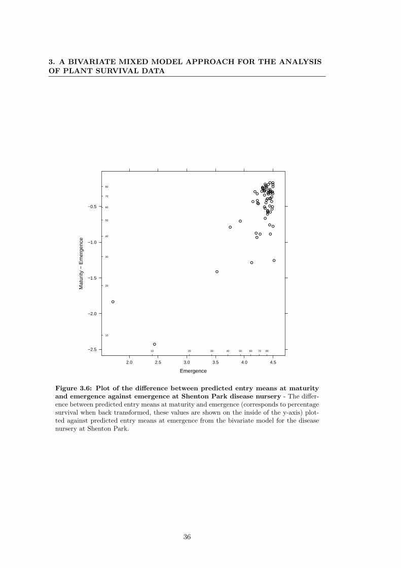
3. A BIVARIATE MIXED MODEL APPROACH FOR THE ANALYSISOF PLANT SURVIVAL DATA
Emergence
Mat
urity
− E
mer
genc
e
−2.5
−2.0
−1.5
−1.0
−0.5
2.0 2.5 3.0 3.5 4.0 4.5
●
●
●
●
●●
●
●
●
●
●
●
●
●
●
●
●
●
●
●
●
●
●
●
●
●
●
●
●
●
●
●
●
●
●
●
●
●
●
●
●
●
●
●●
●
●●
●
●
●
●
●
●
●
●
●●
●
●●●
●
●
●
10 20 30 40 50 60 70 80
10
20
30
40
50
60
70
80
Figure 3.6: Plot of the difference between predicted entry means at maturityand emergence against emergence at Shenton Park disease nursery - The differ-ence between predicted entry means at maturity and emergence (corresponds to percentagesurvival when back transformed, these values are shown on the inside of the y-axis) plot-ted against predicted entry means at emergence from the bivariate model for the diseasenursery at Shenton Park.
36

3.4 Bivariate analysis
Emergence
Mat
urity
− E
mer
genc
e
−3.5
−3.0
−2.5
−2.0
−1.5
−1.0
3.2 3.4 3.6 3.8 4.0
●●
●
●
●
●
●
●
●
●
●
●
●
●
●
●
●
●
●
●
●
●
●
●
●
●●
●
●
●
●●
●
●
●
●
●
●
●
●
●
●
●
●
●
●
●
●
●
●
●
●
●
●
●
●
●●
●●
● ●
●
●
●
●
●
●
●
●
●
●
●
●
30 40 50
10
20
30
40
50
60
Figure 3.7: Plot of the difference between predicted entry means at maturityand emergence against emergence at Wagga Wagga disease nursery - The differ-ence between predicted entry means at maturity and emergence (corresponds to percentagesurvival when back transformed, these values are shown on the inside of the y-axis) plot-ted against predicted entry means at emergence from the bivariate model for the diseasenursery at Wagga Wagga.
37

3. A BIVARIATE MIXED MODEL APPROACH FOR THE ANALYSISOF PLANT SURVIVAL DATA
Tab
le3.6
:T
he
accura
cyof
pred
iction
foreach
trait;(lo
g)
emerg
ence,
(log)
matu
rityan
dth
ed
ifferen
ce(log
matu
ritym
inu
slog
emergen
ce)avera
ged
for
allva
rietiesat
each
sitefor
the
un
ivaria
tean
aly
ses.T
he
evencolu
mn
sin
dicate
the
percen
tage(%
)in
creasein
accu
racy
observed
un
der
the
bivariate
mod
elfor
the
trait.
Location
Em
ergen
ce%
Imp
rovemen
tM
aturity
%Im
provem
ent
Diff
erence
%Im
provem
ent
Un
ivariateE
mergen
ceU
nivariate
Matu
rityU
nivariate
Diff
erence
Bakers
Hill
0.8
40.19
0.5414.13
0.425.63
Clear
Lake
0.870.16
0.890.02
0.870.14
Sh
enton
Park
0.9
70.08
0.960.15
0.910.79
Wagg
aW
agga
0.841.40
0.890.30
0.861.14
Won
won
dah
0.5
810.61
0.850.27
0.850.89
York
0.7
61.21
0.830.00
0.730.93
38
3.5 Discussion
3.5 Discussion
One of the main features of the bivariate approach is the ability to model spatial
variation for each trait. From the results, the components of spatial variation (Gilmour
et al., 1997) differed between the two traits with global trend and extraneous variation
components being added in 5 out of 6 disease nurseries. Local stationary trend also
varied across disease nurseries for each trait with the largest difference between trait
models observed for the York disease nursery (Table 3.3). Another component of the
bivariate analysis is the ability to determine trait-based outliers. It was found that
the number of outliers removed from the analysis differed between traits, with only
one disease nursery having the same numbers of outliers removed for each trait (Table
3.3). These results clearly show that each trait has its own spatial trend and hence
should be modeled individually. Previously such spatial trend differences were not
observed under the historical approach as the use of a ratio of the two plant counts
(percent survival) would have confounded the sources of error of each of the traits. The
differences in spatial distributional properties and outliers between traits is expected as
the error associated with each set of the plant counts/sampling times arises from human
counting error as well as biological and environmental differences that are specific for
each sampling time. In terms of error, it is stated in the NBG protocol that the
emergence counts are to be taken after ‘total germination’, that is the open cotyledon
stage, and before plant death from blackleg disease. However this ‘window’ of time is
not perfect, as plant counts may be taken before total germination and so not all the
plants are counted. The maturity counts according to the protocol, are taken before
the windrowing stage, as it is difficult to determine plant death due to blackleg or
senescence. In addition plants are not counted at maturity if they lean more than 45◦
and if they are not infected by blackleg. As both these counts are based on visual
scores, which are prone to human error there is a different type of error associated with
each sampling time, and this is more accurately modeled under the bivariate analysis.
The error correlation between traits in the bivariate analysis was moderate, averag-
ing at 0.46 across disease nurseries. This represents the repeated measures nature of
the data set, where counts at the different sampling times are taken on the same plot.
Hence while the errors associated with the two sampling times might arise from different
39
3. A BIVARIATE MIXED MODEL APPROACH FOR THE ANALYSISOF PLANT SURVIVAL DATA
sources, they are still moderately correlated. The univariate analysis effectively ignores
this covariance that arises between repeated measures. The bivariate framework is the
preferred method of analysis for plant survival data sets, as it considers each measure
(sampling time) as a realization of an individual trait, thereby enabling the modeling
of covariances between errors.
The current disease nursery protocols require plots with less than 20 counts at
emergence to be omitted and plots with greater than a 100% survival to be truncated
to 100% (Marcroft, 2009). The main reason for the former was to account for entry
plots sown with a poor seed source, and the latter ensured that survival values were
not over 100% as these had no biological meaning. Such values arise due to error, and
under the historical approach these protocols would have resulted in a loss of data from
21% of the total number of plots at the York disease nursery - a substantial loss of data.
Under the bivariate approach such protocols are avoided, as the analysis accommodates
error variation for each of the traits, enabling all data points to be included in the
analysis. Additionally, if the researcher still wants to discount entries with less than
20% emergence this can be done after the analysis. This is a more informed approach
than deletion of the raw data under the historical approach.
The bivariate analysis also allowed for examination of the entry variance for each
of the traits. It was observed across all disease nurseries and traits that the entry
variance was non-zero. Further, the entry variance for maturity was always larger than
that of emergence (Table 3.5). More importantly the bivariate analysis demonstrated
that there is variation across entries for emergence and that this differed across the
disease nurseries, see plots of Wagga Wagga (Fig. 3.7) and Shenton Park (Fig. 3.6).
The entry variance for maturity counts can be safely attributed to the effects of
resistance to blackleg disease, as all other impacts of pests and disease were minimized in
the disease nursery management protocols (Marcroft, 2009). The variation in emergence
counts however could be due to either resistance to early blackleg infection or differences
attributed to variable seed sources across disease nursery locations. Early blackleg
disease infection has been demonstrated to impact on seedling emergence (Li et al.,
2007, Sosnowski et al., 2006). The study by Li et al. (2007) demonstrated that soil
borne ascospores and pycnidiospores of Leptospheria maculans caused seedling death
40

3.5 Discussion
from early infection, resulting in a seedling death rate as high as 59% of seedlings after
sowing in infested soil. Hence the differences in entry emergence attributable to early
infection would constitute genetic effects of resistance.
The existence of genetic variance for emergence counts also raises issues with the
use of the historical method of analysis, which is similar to analyzing maturity counts
with emergence counts as a covariate, commonly known as an analysis of covariance
(Cochran, 1957). In this particular data set, such an analysis will result in maturity
counts being adjusted to a common emergence value, often the average value across all
entries. This not only has the potential to ‘create’ varieties that don’t exist, but this
effectively ‘hides’ the impact of blackleg at emergence. This will be covered in more
detail in Chapter 4.
Seedling emergence is known to be affected by environmental factors such as soil
fertility, salinity, compaction, tillage and surface residues (Forcella et al., 2000). It can
also be affected by seed lot factors such as age of seed (Finch Savage, 1986), the storage
environment of the seed (Ellis and Roberts, 1980), and seed production environment
(Ellis et al., 1993). An illustration of this variance in emergence at a disease nursery
site is evident from the plot of percent survival plotted against emergence at Shenton
Park (Fig. 3.6). At this site, the emergence counts observed were the highest across
all disease nurseries in the data set. When this was queried with the disease nursery
manager it was found out that the disease stubble was distributed on top of plots
after emergence (Dr. Cameron Beeck, pers.comm.), so plots were not sown into disease
stubble. Hence at this particular disease nursery the plots with poor emergence counts
can be directly attributed to poor seed sources and not to early infection of blackleg
disease. Seed source variation is a known issue for Australian blackleg disease nurseries,
however the impact of this variation has not been previously quantified.
A key component of the bivariate analysis is the inclusion of a correlation between
entry effects at emergence and maturity. This correlation was strong across the 6 disease
nurseries, averaging 0.74 with a range of 0.71 to 0.94 (Table 3.5). A high correlation
between entry effects indicates a strong agreement between entry rankings for both
the traits. That is, regardless of the different causes of the variation at emergence
and maturity, they are still strongly correlated at most disease nurseries. Thus the
41

3. A BIVARIATE MIXED MODEL APPROACH FOR THE ANALYSISOF PLANT SURVIVAL DATA
bivariate analysis enables further insights into plant pathogen interactions, which would
otherwise not be observed under the historical analysis.
Another key (statistical) motivation of the bivariate analysis is the increases in
accuracy afforded by multi-trait predictions. The results from the 6 disease nurseries
show that there are improvements in prediction accuracies under the bivariate model
for the emergence and maturity traits and also for the difference which is particularly
important since it is analogous to the trait of percent survival as used in the historical
approach. While the improvements are modest within this data-set, the gains for any
particular data-set are obviously unknown prior to an analysis but may be larger than
reported here and are worth pursuing given that there is little extra cost or difficulty
involved in conducting the bivariate analysis.
For entry selection, the bivariate approach provides a more detailed picture; a two
dimensional representation of disease impact not provided by the historical approach.
The analysis enables the prediction of entry means at emergence and maturity, which
can be used to generate three sources of information for selection: emergence counts,
maturity counts and percentage survival values. Additionally, this study demonstrates
that if percent survival values are preferred as the trait for selection, this should not
be done without reference to emergence counts. This is because biologically each set of
plant counts is affected by different biological, genetic and environmental impacts.
3.6 Summary
This chapter presents an approach for a bivariate mixed model analysis of plant survival
data from designed field trials. In the motivating data set the two variables subject to
analysis are the two ‘traits’; plant survival counts taken at emergence and at maturity
sampling times. This method is not only an improvement over the historical method for
analyzing a derived variable ‘percent survival’ but demonstrates how entries can still be
assessed according to the historical selection basis (percent survival) in a more accurate
manner. Additionally this analysis method encompasses the differences between traits,
which are clearly affected by different biological, genetic and environmental influences.
The bivariate approach provides a more detailed picture for entry selection for blackleg
42

3.6 Summary
resistance than the historical approach. E-BLUPs of entry means at emergence and
maturity can be used to generate three sources of information for the basis of selection,
namely emergence counts, maturity counts and percentage survival values. The next
chapter will discuss other potential applications of bivariate analyses for plant breeding
data.
43

3. A BIVARIATE MIXED MODEL APPROACH FOR THE ANALYSISOF PLANT SURVIVAL DATA
44

Chapter 4
Further applications of bivariate
analysis for plant breeding data
4.1 Introduction
Plant breeding programs rarely carry out selection for one trait at a time, as breeding
objectives commonly involve the selection of multiple traits concurrently. However there
are very few examples of multivariate trait analysis in plant breeding trials (Piepho
et al., 2008), yet it is commonly utilized in animal and forestry trials (Balestre et al.,
2012). Instead, plant breeding trials commonly utilize either a multi-trait index for
selection or covariance analysis to analyze for a single trait while ‘adjusting’ for the
presence of another trait. In Chapter 3 it was briefly outlined how covariance analysis
may be biologically and statistically inferior in comparison to a bivariate analysis. In
this chapter the pitfalls of covariance analysis are discussed by reviewing a select set of
previous studies in plant breeding which utilize such an analysis, and contrasting these
with the bivariate analysis. This review also highlights further selection applications
in plant breeding where bivariate methods may be beneficial.
Analysis of covariance, also referred to as ANCOVA, was introduced by Fisher in
1934. The most common uses of ANCOVA in agricultural studies include the removal
of extraneous variation that is not controlled by experiment design or the adjustment
of treatment means by a covariate value for ‘suitable comparisons’ (Yang and Juskiw,
45

4. FURTHER APPLICATIONS OF BIVARIATE ANALYSIS FORPLANT BREEDING DATA
2011). Since the introduction of ANCOVA in 1943, there have been numerous papers
published that warn against the misuse of this analysis method; see discussions by
Cochran (1957), Smith (1957), Urquhart (1982). Nevertheless there are still a large
number of plant breeding studies that routinely use this form of analysis.
Using the notation of Smith (1957), ANCOVA is commonly summarized in the form
of
yij = µ+ τi + βxij + εij (4.1)
Here, yij and xij are the jth observation on the ith treatment of the dependent variate
and covariate (Smith, 1957). τi is the effect of the ith treatment, µ is the grand mean,
β is the slope of the regression on the covariate and εij is the random error. The
main assumptions for use of ANCOVA are (i) the covariate must be measured without
error, (ii) the covariate must not be affected by any treatment and (iii) the slope of the
regression line is the same for each treatment (Elashoff, 1969). In most of the studies
reviewed in this chapter, the misuse of covariance analysis is discussed with respect to
assumption (ii), which a majority of studies fail to meet.
This chapter consists of a review of plant breeding studies in the areas of disease
resistance and grain yield, which both utilize covariance analysis. Also considered is
a section on Quantitative Trait Loci (QTL) studies in the areas of disease resistance,
grain yield and protein content, which also commonly use covariance adjustment.
4.2 Breeding for disease resistance
Breeding for disease resistance is an important component of cultivar production, as it
is an effective method of ensuring yield stability. The studies reviewed in this section
consider experiments, which select for disease resistance. For the disease resistance
trait, covariance analysis is often used to adjust for other traits such as emergence
levels, heading date and mould levels.
46
4.2 Breeding for disease resistance
4.2.1 Adjustment for seedling emergence
Disease incidence data is commonly expressed as the proportion of disease units out
of a total amount, and is often represented as a percentage. The blackleg data set of
Chapter 3 is a form of disease incidence data as plant counts are taken at emergence
and maturity and used to construct the variable percent survival,
maturity
emergence× 100 = %survival (4.2)
In the blackleg plant breeding experiment, the aim is to determine the treatment im-
pact (variety resistance) under disease pressure. In this case the historical analysis is
analogous to an analysis of covariance where the response variable, maturity counts,
are analyzed using the emergence counts as a covariate, but with the slope fixed at one.
However, in Chapter 3 it was demonstrated that the individual plant counts have dif-
ferent biological, environment and genetic differences, constituting two separate traits,
which would be more accurately analyzed under a bivariate framework of analysis. It
was also demonstrated for the blackleg data set of Chapter 3, that there exists genetic
variance for emergence. This could either be due to differential blackleg at emergence
(Li et al., 2007, Sosnowski et al., 2006) or due to differences that arise in seed lots
(Finch Savage, 1986). If it is due to the former, it implies that the covariate is af-
fected by the treatment, which invalidates a key assumption of covariance analysis.
As a result, covariance analysis could in fact misrepresent the real treatment effect
by adjusting out the part of the treatment effect which results in the covariate in the
first place (Urquhart, 1982). Another limitation with covariance analysis is that, the
analysis adjusts maturity means to a common emergence level, typically the site mean
(Smith, 1957). This not only eliminates the impact of blackleg at emergence, it also
implies that it is possible for each variety to attain this ‘mean’ level of emergence. This
effectively creates ‘new’ varieties, which may not exist (Smith, 1957).
4.2.2 Adjustment for heading date
The study by Emrich et al. (2008) on Fusarium head blight resistance in wheat cultivars,
was based on covariance analysis to adjust for heading date (HD). This aimed to avoid
47

4. FURTHER APPLICATIONS OF BIVARIATE ANALYSIS FORPLANT BREEDING DATA
the selection of late heading genotypes, which tend to develop less head blight due
to a much shorter vegetative period. The covariate and the response variable were
measured on the same experimental unit; field plots of a variety. This poses issues
for the interpretation of the results, as the adjustment to a common heading level is
meaningless - HD is a variety specific characteristic that cannot be adjusted. The
authors acknowledge this, but argue that such an adjustment is acceptable as they test
varieties from similar earliness classes, resulting in similar heading dates anyway.
The use of HD as a covariate in the study by Emrich et al. (2008) is not biologically
valid for two main reasons. The first is that heading date is a major trait of selection
critical for regional and seasonal based adaptation of wheat cultivars (Zhang et al.,
2009). Covariance adjustment creates a common HD, which is not only biologically
incorrect but also impedes the selection of this trait. The second reason arises because
the genetic background of the cultivar and environment can affect the heading date
(Stelmakh, 1992). HD is known to be under polygenic gene control, controlled by
three categories of genes: vernalization response, photoperiod response and earliness
per se (Stelmakh, 1992, Zhang et al., 2009). Further it is also affected by environmental
conditions such as day length and temperature (Zhang et al., 2009). Considering these
factors, HD is clearly a trait with its own genetic variance and thus should not be used
as a covariate.
4.2.3 Adjustment for fungal mould levels
The study by Atlin et al. (1983) developed a method for selecting corn hybrids for
resistance to the fungal pathogen Gibberella zeae, which is known to be the cause of
ear rot. Six corn hybrids were tested for two factors; the first was the level of ear
rot and the second is the mycotoxin levels that result from Gibberella zeae produced
metabolites. The latter was important in this study, as mycotoxins are toxic when
consumed by cattle. Covariance analysis was used to adjust mycotoxin accumulation
for the level of Gibberella zeae mould. However, the analysis resulted in no significant
differences in toxin accumulation in either of the years the trials were run.
This study is also an example where there are differences of the covariate imposed
with treatments. For example, the treatments in this experiment are the six corn
48

4.2 Breeding for disease resistance
varieties, with each having a different response to disease infection. So it is unknown
if the variation in mould levels can be directly attributed to the corn variety or a
combination of biological, environmental and genetic factors. Adjustment to a common
Gibberella mould level is in general an adjustment to an environment condition specific
to infection, i.e it is impossible to associate a set of factors to enable a particular level
of fungal infection. This is mainly due to varieties having different genetic responses
to mould infection and level of toxin production. As a result the use of mould level as
a covariate is not accurate for the selection objective of this study.
4.2.4 Adjustment for plant stand and days from planting
In the study by Littley and Rahe (1987), disease levels in onions from white rot (Scle-
rotium cepivorum Berk.) were analyzed using plant density level as a covariate. The
motivation for this being that plant density is known to impact on host plant disease
levels. Like some of the above examples, the covariate could be affected by the treat-
ment (varieties), as some varieties may have a higher density than others for many
reasons. As a result adjustment of disease levels for the covariate, might adjust out
the impact of disease levels on varieties. The authors state that they only used means
adjustment for trials that were significant under an ANCOVA, which also did not show
significant differences for slopes between treatments. However, this was only the case in
3 out of the 6 trials. For one of the three trials where ANCOVA was significant, means
adjustment led to no significant difference among varieties, when there were significant
differences under an ANOVA. Thus, the use of covariance analysis may not have been
statistically valid.
In this study, as well as the study by Atlin et al. (1983), there are differences in
the covariate for the imposed treatments. In particular, consider that the treatments
are the different varieties tested, with each having different plant density based on the
variety morphology. In this case adjustment to a common plant density is misleading
as it is not possible to know if plant density alone impacts on disease levels, or if there
is a combination of genetic, environmental and biological factors that has an impact
on disease levels. Plant stand can be affected by any number of factors. Environmen-
tal conditions in the field can impact the number of plants emerged (Forcella et al.,
49

4. FURTHER APPLICATIONS OF BIVARIATE ANALYSIS FORPLANT BREEDING DATA
2000), and seed characteristics such as seed source differences can impact stand number
achieved (Finch Savage, 1986). In addition plant stand can also be viewed as a genetic
effect, as it is also impacted by disease. Littley and Rahe (1987) state that the disease
has been known to directly cause damping off and seedling loss, especially at the Grand
Forks site. The use of covariance adjustment to a common stand level in this case, is
biologically meaningless.
4.3 Breeding for grain yield
Grain yield is the main trait for selection in field crops, with the aim to surpass the
current levels of commercial varieties. Studies reviewed in this section examine the
selection of grain yield, while using covariance analysis to adjust for factors such as
plant stand and grain moisture content.
4.3.1 Adjustment for plant stand
The study by Kamidi (1995) aimed at selecting high grain yielding maize varieties, while
accounting for incomplete plant stands in agronomy field trials. Covariance analysis was
used to analyze grain yield with plant stand number as a covariate, thereby obtaining
treatment effects that are comparable across varying numbers of plot stand. While the
author states that this adjustment is often satisfactory, he found that this adjustment
might not be acceptable when plants are missing at germination and before maturity
as competition effects invalidate linear covariance adjustment. The authors instead
suggest the use of an exponential model to correct for plot stands and contrast the
results from this analysis with those obtained from covariance adjustment.
Kamidi (1995) used covariance analysis in an identical way to the example outlined
by Smith (1957) where maize grain yield was analyzed with stand number as a covariate.
In his review on the interpretation of adjusted means, Smith (1957) argues against the
use of plant stand to adjust for yield variations, arguing that stand form is an integral
part of the treatment effect. This is primarily because it is not possible to determine
if variations in grain yield are directly attributable to plant stand number or due to
variations in fertility in the field as well (Smith, 1957). Hence if covariance analysis
50
4.3 Breeding for grain yield
is used, the adjustment no longer removes a component of the experimental error and
more importantly distorts the real treatment effect measured (Cochran, 1957). The use
of covariance analysis to obtain adjusted means for grain yield effectively assumes that
all the varieties tested can achieve this plant stand number. Like the above examples,
it is biologically incorrect and results in the creation of varieties that do not exist.
Pixley and Bjarnason (2002) screened a series of quality protein maize cultivars
for the assessment of the traits grain yield, protein content, quality and endosperm
modification (translucent or near normal phenotype). These cultivars consisted of
three-way cross, double cross and open pollinated varieties which were grown across
three tropical locations in four continents. Covariance analysis was used in this study to
adjusted grain yield for plant stand at two of the sites in Thailand, Tak Fa and Suwahn.
This was mainly because plant stand at Suwahn was affected by water logging, and at
Tak Fa was severely affected by downy mildew, resulting in diseased seedlings. Across
location analyses used these covariance-adjusted means from these two sites along with
the raw, lattice-adjusted means from the other sites. The use of covariance analysis
may have been inappropriate in this study because at both the sites plant stand could
be considered a trait in its own right.
4.3.2 Adjustment for grain moisture levels
The majority of above ground dry matter of corn is commonly referred to as stover
and is used as animal feed. Stover is usually allowed to dry above ground, however
weather conditions in Ontario prevent drying to prescribed moisture levels required for
dry feed storage (Leask and Daynard, 1973). Cultivars used for stover production are
thus selected to have a high rate of moisture loss before and after harvest - referred
to as stover quality. The study by Leask and Daynard (1973) tested the variability
among commercial corn hybrids in stover quality and yield. The traits grain yield and
dry matter yield were covariance adjusted to 15.5% moisture and 30% grain moisture
respectively.
The use of grain moisture as a covariate may not be acceptable as it is a trait that
is selected for, which in turn implies that it will have its own genetic variance. Further
Leask and Daynard (1973) and another study by Pordesimo et al. (2004) state that
51

4. FURTHER APPLICATIONS OF BIVARIATE ANALYSIS FORPLANT BREEDING DATA
differences in stover moisture content results from the variations in the date at which
the cultivars started drying below the initial moisture content. Clearly this implies that
drying below initial moisture content is a genetic characteristic of a particular variety,
which is affected by maturity date. Thus, adjusted means for grain moisture has little
biological meaning, as not all varieties can achieve this level.
4.4 QTL analysis - adjusting for other traits
A number of studies that routinely use covariance analysis are found in the area of
Quantitative Trait Loci (QTL) studies. A subset reviewed in this section includes
studies in the areas of disease resistance, grain yield, and end use quality traits in
wheat and barley breeding.
Klahr et al. (2007) studied a population of wheat recombinant inbred lines (RILs),
to determine QTLs for FHB resistance in wheat. The additional traits plant height
(PH) and heading date (HD) were also measured to determine correlations with FHB
resistance. Disease infection was measured in terms of percent of infected spikelets
(visual score), which were scored over multiple day intervals. These scores were then
used to calculate the area under the disease progress curve (AUDPC) for each plot
and environment. In cases where a significant correlation between FHB and PH or
HD existed the visual scores were adjusted using a covariance analysis. These adjusted
scores were then used for scanning FHB QTLs.
As discussed previously for the study by Emrich et al. (2008), HD is not a valid
covariate as it is a trait itself impacted by different genetic and environmental factors.
Similarly PH is another important trait of selection for wheat breeders, as it represents
a compromise between plant density requirements and lodging resistance (Zhang et al.,
2008). PH is also a morphological characteristic of a particular variety, and known to
be under polygenic control (Cadalen et al., 1998). Thus the adjustment for PH and
HD is not biologically meaningful, as these are inherent characteristics of a particular
genotype, and so any resulting adjustment has the potential of creating varieties that
do not exist. Further the use of these traits as a covariate also ‘covers’ the impact of
52

4.4 QTL analysis - adjusting for other traits
these on FHB resistance, which will have a detrimental impact on selection for FHB
resistance.
In rice QTL studies it is common to use days to flowering (DTF) as a covariate for the
analysis of grain yield. This is the case in both the studies Venuprasad et al. (2009) and
Vikram et al. (2011). Venuprasad et al. (2009) used rice RILs from the cross of varieties
Apo and Swarna to detect QTL’s for grain yield under drought stress. The effect of
days to flowering (DTF) was adjusted for grain yield for the different marker classes,
based on covariance analysis. Vikram et al. (2011) similar to Venuprasad et al. (2009)
identifies QTLs for grain yield in rice under stress however during the reproductive
period in a F3 mapping population produced from crosses of N22 with IR64, Swarna
and MTU1010. To eliminate DTF and as well as PH effects on grain yield, grain yield
was analyzed using covariance analysis with DTF and PH as covariates. Predicted
grain yields after covariate analysis was then used for marker analysis.
The use of covariance analysis to adjust for DTF in Venuprasad et al. (2009) and
DTF or PH in Vikram et al. (2011) is inaccurate as the adjustment for such traits is
unrealistic given that these are inherent characteristics of a particular variety. As a
result any adjustment to a common level is not biologically meaningful, as it is clear
that not all varieties can achieve this. DTF is a key trait selected for in rice breeding,
as it indicates the maturity class of a variety. Both DTF and PH are known to be
under polygenic inheritance (Li et al., 1995). Further, both traits are impacted by
environment; with the study by Li et al. (2003) finding that genotype by environment
interaction (GxE) has more of an impact on HD than on PH when examining QTLs for
these respective traits. Hence DTF and PH are traits in their own right and will have
their own genetic variance implying their use under covariance analysis is inaccurate.
Breeding programs in wheat and barley include breeding objectives for the selection
of end use quality traits. For wheat, these traits include dough rheological characters,
and for barley these include malting quality attributes. In the following studies reviewed
these traits are often adjusted for protein content, whether it is grain protein content
(GPC) or flour protein content (FPC), due to negative correlations between these
traits with other end use traits. It is thus common in wheat and barley programs to
53
4. FURTHER APPLICATIONS OF BIVARIATE ANALYSIS FORPLANT BREEDING DATA
use covariance adjustment for GPC values while selection for yield and malting quality
traits are undertaken (Blanco et al., 2012, Emebiri et al., 2004).
Blanco et al. (2012) studied QTLs for GPC in a RIL population of 120 durum wheat
lines. These lines were derived from the cross between Svevo and Ciccio and trialed
across 5 environments in southern Italy. GPC data from this study was covariance
adjusted for each of the yield components: grain yield per spike (GYS), thousand-kernel
weight (TKW) and kernel number per spike (KNS) due to the negative correlation
between GPC and yield components. Ten genomic regions were identified as being
involved with GPC expression and 6 of these were associated with one or more grain
yield component QTL.
Kuchel et al. (2006) studied a Double Haploid (DH) population from the cross of
Trident and Molineux, to investigate end use quality traits and QTLs for dough rheo-
logical traits. These included flour protein (FP), particle size index (PSI), flour yield
(FY), and other baking quality traits (in total 14 traits). If there was a significant cor-
relation between two traits, an adjusted value was calculated using covariance analysis
and used for QTL mapping. FP was found to be correlated to grain yield, and so FP
was adjusted for grain yield (GY) using covariance analysis. This study identified QTL
associated with FP from the adjusted GY data, which were not identified when using
the unadjusted data.
Emebiri et al. (2004) studied QTLs impacting barley malting quality attributes,
across 180 DH lines produced by crossing parents with low GPC. Covariance analysis
was used to adjust malt extract and diastatic power attributes for GPC. Single QTL
scans were repeated for both these adjusted values. The authors found that covariance
adjusted GPC values resulted in an increased number of QTL identified for malt extract
and diastatic power
In the above QTL studies the issue with covariate analysis is that the covariate is a
trait in its own right, which is commonly selected for in a breeding program. As such
it will have its own genetic variation, and this is the main factor that precludes its use
in covariance analysis.
54
4.5 Discussion
4.5 Discussion
A key assumption of covariance analysis is that the covariate should not be affected
by the treatment. In the studies reviewed above, it is most likely that the covariate
is affected by the treatment as it is often a trait that is also selected for, which would
imply that it will have its own genetic variance. When this particular assumption
is violated the interpretation of results should be treated with caution, as covariance
analysis no longer reduces that component of experimental error, attributed to the
covariate and also alters the nature of the treatment effect measured (Cochran, 1957,
Urquhart, 1982). This is one of the main reasons why this form of analysis has been
historically warned against (Smith, 1957, Urquhart, 1982).
Additionally for all of the studies reviewed above, it could be argued that covariance
adjustment is not biologically accurate, as the adjustment in most cases led to a common
level which some varieties in the experiment could not achieve, hence ‘creating varieties’
(Smith, 1957).
Both the limitations mentioned above are easily avoided using a bivariate analysis.
A bivariate analysis would be more appropriate for these studies, as the covariate and
response variable are treated as two separate traits. This has additional benefits in
terms of selection, as the bivariate analysis enable a two-dimensional view for the selec-
tion of varieties based on the two predicted traits without the need for an adjustment.
Thereby it is a more flexible framework of analysis as under the bivariate analysis the
covariate can be incorporated into the selection process. This is especially the case with
the study by Emrich et al. (2008), where a bivariate analysis will enable predictions
for both FHB resistance and heading date, enabling conditional selection for FHB re-
sistance for a lower heading date. Thus, there is no need to specify analysis classes of
similar heading date genotypes under a covariance analysis.
Another assumption of the covariance analysis is that the covariate should be mea-
sured without any error. However in practice this is near impossible. The bivariate
framework however enables the modeling of spatial error for each trait, which is effec-
tively ignored under covariance analysis. As demonstrated in the blackleg motivational
data set in Chapter 3 the modeling of spatial error for emergence and maturity traits
55

4. FURTHER APPLICATIONS OF BIVARIATE ANALYSIS FORPLANT BREEDING DATA
encompasses the different sources of error that could arise from the measurement of
each trait. Furthermore, spatial modeling has been demonstrated to result in greater
accuracy in estimation of treatment effects (Cullis et al., 1998, Smith et al., 2002a,
2001b) and a reduction in error variance, leading to increases in prediction accuracy
(Dutkowski et al., 2006). Hence the treatment of the covariate and the response variable
as individual traits would allow for the fact that there are multiple factors contributing
to error variation in each.
The bivariate framework of analysis also allows for a genetic covariance structure
between traits, which is ignored under the covariance analysis. Hence the bivariate
analysis would avoid any bias in evaluation which could arise by ignoring covariance
structures between traits (Lin et al., 1985). This has been demonstrated by the study
of Korol et al. (1995), who found that joint treatment of correlated traits, may provide
better power of detection and higher precision of parameter estimation for linked QTLs
than single traits. In addition under a bivariate analysis, utilizing information from
genotypic correlations can often lead to increases in the accuracy of evaluation (Mrode
and Thompson, 2005, Thompson and Meyer, 1986). This is especially the case when
traits are known to be highly correlated, which is the case with FHB and PH or HD
in the study by Klahr et al. (2007) and GPC or FPC with other end use traits in the
studies by Blanco et al. (2012), Emebiri et al. (2004) and Kuchel et al. (2006).
4.6 Summary
There are numerous examples of plant breeding experiments that use ANCOVA ap-
proaches for adjusting one variable for another. In this chapter some of these studies
have been reviewed and it has been shown that in all cases ANCOVA was inappropri-
ate and that a bivariate analysis of the form described in Chapter 3 may have been
preferred.
56

Chapter 5
Literature Review - Pedigree
information in plant breeding
METs
5.1 Introduction
Plant breeding varieties are routinely evaluated in series of trials known as multi-
environment trials (METs) to evaluate variety performance at a range of locations
and years, where locations and years can be synonymous with variable growing seasons
(Frensham et al., 1997, Kelly et al., 2007). MET trial data, consisting of phenotype
and pedigree information, can be included in linear mixed models to obtain genetic
values including breeding values at each location (Beeck et al., 2010, Burgueno et al.,
2007, Crossa et al., 2006, Cullis et al., 2010, Oakey et al., 2007). In contrast to animal
breeding, very few plant breeding programs base their selection on breeding values,
and Piepho et al. (2008) indicated that this type of analysis is limited to research.
Recently, the benefits of MET data analysis with pedigrees was demonstrated inside a
commercial breeding program (Beeck et al., 2010, Cullis et al., 2010). Selection based
on breeding values is known to outperform other commonly used selection strategies
especially in cases where data sets are unbalanced, have large pedigrees, or low trait
heritability (Bauer et al., 2009).
57
5. LITERATURE REVIEW - PEDIGREE INFORMATION IN PLANTBREEDING METS
Animal breeders have used mixed model methodology to exploit large series of phe-
notypic and pedigree data and BLUPs for the prediction of breeding values as the basis
of selection (Henderson, 1973, 1975). Bernardo (1994, 1995) applied this to crop breed-
ing, using mixed models and Restriction Fragment Length Polymorphisms (RFLP)
estimations of relationships to obtain BLUP breeding values of hybrid maize entries.
Compared with animal breeding, plant breeding trials have the additional complexity
of varieties being tested in replicated plots which impacts on experimental design and
analysis, but allows for the exploration of non-genetic effects and non-additive genetic
effects when pedigree information is included. Further, crops have the added complex-
ity of trials being conducted across multiple environments which enables the testing of
GxE.
MET analysis provides estimates of the magnitude and patterns of GxE on additive
and non-additive genetic effects when pedigree information is included (Cullis et al.,
2010, Kelly et al., 2009, Oakey et al., 2007). GxE interactions can be differentiated
by (i) interactions that arise due to heterogeneity of genetic variance among environ-
ments (Fig. 5.1b) and (ii) the lack of genetic correlation among environments (Fig.
5.1c) (Cooper et al., 1996). Cross-over GxE represents the failure of varieties to rank
uniformly across environments for that trait (Figs. 5.1c & 5.1d) (Basford and Cooper,
1998). Biologically, GxE occurs when the contribution of gene expression for an entry
varies according to the environment (Basford and Cooper, 1998). GxE limits the re-
sponse to selection, as entries vary in their performance over environments (Argillier
et al., 1994, Cooper and DeLacy, 1994), thereby reducing the efficiency of plant breed-
ing. Alternatively, if patterns of GxE were better understood, it might be possible to
improve the efficiency of plant breeding, especially if genetic relationships were known
(Beeck et al., 2010, Cullis et al., 2010).
In the case of F1 hybrid breeding the most expensive step is the identification of
parental combinations that produce F1 hybrids with superior agronomic traits (Riaz
et al., 2001). It is difficult to assess the breadth of adaptation of a new variety without
exposing it to a wide range of environments. Thus, from a breeder’s perspective it is
important to be able to determine the GxE effects on parental combinations early in
the testing program, and to predict the adaptation range of new hybrid varieties.
58

5.1 Introduction
Environment
Gra
in y
ield
(t/h
a)
2
3
4
5
6
7
E1 E2
(a)
Environment
Gra
in y
ield
(t/h
a)
2
3
4
5
6
7
E1 E2
(b)
Environment
Gra
in y
ield
(t/h
a)
2
3
4
5
6
7
E1 E2
(c)
Environment
Gra
in y
ield
(t/h
a)
2
3
4
5
6
7
E1 E2
(d)
Figure 5.1: Schematic representation of two entries (blue = entry 1 and pink = entry 2)and their performance across two environments: (a) no GxE; (b) GxE due to heterogeneityof variance between the environments but not lack of genetic correlation; (c) GxE due tolack of genetic correlation but not heterogeneity of variance between environments; (d)GxE due to heterogeneity of variance between the environments and the lack of geneticcorrelation. This diagram has been reproduced from Cooper et al. (1996).
59

5. LITERATURE REVIEW - PEDIGREE INFORMATION IN PLANTBREEDING METS
In hybrid breeding programs, parental selection has been based traditionally on
general combining ability (GCA), which predicts the average performance of a parent
in hybrid combinations in designed experiments (such as a diallel cross) and is often
assumed to be due to additive effects (Can et al., 1997, Lynch and Walsh, 1998). Wricke
and Weber (1986) indicate that the GCA is dependent on the tester population. In the
case of diallel crosses, the tester population is the population itself, and the GCA of the
parent is half the breeding value of the parent. With other tester populations, there
is a linear relationship between breeding values and GCA (Wricke and Weber, 1986).
Specific combining ability (SCA) is the deviation from prediction based on GCA, and
is assumed to be the result of non-additive gene effects that contribute to heterosis
(Virmani, 1994). It has long been acknowledged that GCA and SCA are subject to
GxE interaction (Kidwell, 1963). In studies of hybrid rice, heterosis for yield has
been shown to vary across parent combinations and across environments (Young and
Virmani, 1990). Most recently, Cullis et al. (2010) showed through pedigree analysis
that additive and non-additive components differed for each trait (oil and grain yield in
canola) and were subject to different GxE effects in both inbred entries and F1 hybrids.
In plant breeding programs, there are two concurrent objectives for the selection of
entries: to select the best parents for crossing, and to select superior future varieties
with improved performance (Liu and Wu, 1998). The estimation of additive and non-
additive components of entry performance in plant breeding trials potentially improves
parental selection and selection of future new varieties. The additive component or
‘estimated breeding value’ is the heritable portion of a entry (Lynch and Walsh, 1998),
which is the ability to pass on its genes (Burgueno et al., 2007). Historically, animal
breeders have focused on the estimation of breeding values, with less importance placed
on non-additive effects (Ovaskainen et al., 2008). Non-additive components however,
are important to estimate as ignoring the non-additive covariances can result in the
inaccurate estimation of the additive genetic variance (Du and Hoeschele, 2000, Misztal,
1997).
The purpose of this chapter is to review current methods and approaches for the
inclusion of pedigree data in mixed model approaches for the analysis of plant breeding
data sets. This chapter commences with a review on the applications of pedigree data
in MET data sets, followed by sections which consider pedigree-based and molecular
60

5.2 Analysis of MET trials
marker-based relationship matrices. It is then concluded with areas of current research
which will be examined in the subsequent experimental chapters.
5.2 Analysis of MET trials
5.2.1 Linear Mixed Model Approach
Linear models which jointly account for fixed and random effects are regarded as ‘mixed
models’ (Eisenhart, 1947). Mixed models have been applied to MET analysis of Aus-
tralian crop evaluation trials (Kelly et al., 2007, Smith et al., 2001b, 2005). Smith et al.
(2001a) were the first to develop and apply a factor analytic (FA) mixed model frame-
work for MET data. This particular mixed model approach allowed for heterogeneity
of genetic variance between trials; different patterns of genetic correlations among tri-
als and error variance structures of individual trials in the analysis of MET trial data
(Smith et al., 2001a). The benefits of this framework include the handling of large
unbalanced data sets, estimates of random entry and or environment effects, and esti-
mates of GxE interactions (Smith et al., 2005). FA mixed modeling can also be used
to assess patterns of genotypic adaptation and assist in the identification of groupings
of environments within MET data (Beeck et al., 2010, Cullis et al., 2010).
Historically, mixed model analysis of MET data has always assumed the indepen-
dence of entries (Piepho et al., 2008). This is not a realistic assumption, as in plant
breeding programs, entries tend to be related to each other, such as full sibs, half sibs,
sister lines etc. In a breeding program, the assumption of independence of entries does
not hold since there are often many generations of controlled crossing among selected
entries. Selection results in a genetic covariance from the common backgrounds of
entries within a program, and, by including the relationships between entries, mixed
model approaches can encompass this additional covariance (Malosetti et al., 2011).
Hence mixed model approaches which integrate pedigree information are usually supe-
rior to those that do not (Beeck et al., 2010, Crossa et al., 2006, Oakey et al., 2006,
2007).
Estimates of GCA and SCA are usually obtained through specialized mating de-
signs such as the diallel cross (Mather and Jinks, 1982), which separates the total
61

5. LITERATURE REVIEW - PEDIGREE INFORMATION IN PLANTBREEDING METS
genetic effect of an entry into GCA and SCA. However, such mating designs are re-
source, time and cost intensive, as only a small number of parents and progenies can
be tested, and replication is limited (Oakey et al., 2006). These traditional designs also
assume that the parents are not related, which is not always the case in a breeding
program due to methods of selection (Balzarini, 2002, Bernardo, 1994). Henderson and
Quaas (1976) first utilized pedigree data for the derivation of a additive relationship
matrix within a mixed models setting for the prediction of breeding values (additive
component) in animal breeding. Oakey et al. (2006, 2007) used pedigree relationship
matrices with plant breeding MET trial data to independently estimate entry additive
and non-additive components. Oakey et al. (2006) incorporated mixed model analysis
with pedigree data in single trial analysis of pure line entries to determine additive
and non-additive effects, without the use of specialized mating designs. Both additive
and non-additive values were estimated for pure line entries, whereas SCA can only be
estimated for F1s in controlled mating designs - which demonstrates the limitations of
the GCA/SCA concept in plant breeding. Oakey et al. (2007) extended the MET/FA
mixed model framework of Smith et al. (2001a) to sugarcane; a cloned hybrid crop. In
this case, the non-additive component of entry effects included dominance and resid-
ual non-additive effects; the latter which can arise from inbreeding depression effects,
homozygous dominance effects, the covariance between additive and dominance effects
and epistatic effects (Oakey et al., 2006). This study however, did not distinguish
these latter sources of non-additive components, which may be important in the pre-
diction of heterosis in hybrid crops. Beeck et al. (2010) applied this framework to a
canola breeding program across southern Australia, and demonstrated improved model
fit with pedigree information, and Cullis et al. (2010) examined patterns of GxE for
yield additive and total effects and the further application of prediction and selection
indices for these components. These studies demonstrated that pedigree data can be
routinely included in the analysis of plant breeding trials to obtain breeding values for
parental selection and improved estimates of total genetic value for varietal selection.
Inbred parental entries have both additive and residual genetic components (the lat-
ter is presumably a restricted form of epistasis which results from interactions among
homozygous loci). In F1 progeny, on the other hand, the non-additive component of
genetic variance is due to dominance and epistatic effects (in this case, all types of epis-
62

5.3 Heterosis and GxE
tasis including interactions among heterozygous loci). Within a MET/FA framework
these genetic variances and correlations may need to be summarized separately for in-
bred entries and hybrid progeny. Combined analysis of parents and hybrids has been
accomplished through the use of marker and pedigree based data in maize entries by
Schrag et al. (2010). In this study they used mixed models to determine the prediction
ability of pedigree and molecular based data on hybrid performance, but they did not
use MET/FA framework to analyze the impact of GxE on hybrid performance, and
they ignored potentially large changes in additive and non-additive components across
environments.
5.2.1.1 Prediction models and relationship matrices
There is a great deal of interest in using relationship matrices in mixed models for
the prediction of heterosis in untested hybrids (Bernardo, 1994, 1995, Maenhout et al.,
2010, Schrag et al., 2006, 2009). In the studies by Bernardo (1994, 1995, 1996b,a)
phenotypic scores for each hybrid were obtained from the average of all the phenotypic
measurements, which were then subject to a combined analysis of variance across lo-
cations. Prediction models are not part of this review, as the focus of this research is
the analysis of plant breeding field trials and the partitioning of the field tested entries
into genetic components.
5.3 Heterosis and GxE
The term heterosis, as it applies to plant breeding, was developed by Shull in 1908 and
refers to “an F1 performance that exceeds the average parental performance” (Lynch
and Walsh, 1998). Heterosis is an observed characteristic (Bernardo, 2002), and histor-
ically has been based on observations of total genetic value. However, the underlying
genetic causes of heterosis are the subject of on-going research (Hochholdinger and
Hoecker, 2007). The main causes are assumed to be dominance, over dominance and
epistasis. The dominance hypothesis states that heterosis is based on superior dominant
alleles at multiple loci which mask the unfavourable alleles in the heterozygote (Lynch
and Walsh, 1998). The over-dominance hypothesis states that the heterozygous state
63

5. LITERATURE REVIEW - PEDIGREE INFORMATION IN PLANTBREEDING METS
results in higher phenotypic values than either parental homozygous state (Lynch and
Walsh, 1998). Lastly, the epistasis hypothesis states that interactions between alleles at
different loci result in the manifestation of heterosis (Lynch and Walsh, 1998). Recent
reviews suggest that these three hypotheses are not mutually exclusive (Hochholdinger
and Hoecker, 2007, Lippman and Zamir, 2007). This limited understanding of the ge-
netic basis of heterosis has not limited the exploitation of heterosis for crop breeding,
however it is important in the long term to understand these components of heterosis
in order to predict hybrid performance in plant breeding.
It is difficult to assess the breadth of adaptation of a new hybrid variety without
exposing it to a wide range of environments. Thus, from a breeder’s perspective,
it is important to determine the GxE effects on parental combinations early in the
testing program, and to predict the range of adaptation of new hybrid varieties. This is
demonstrated in recent studies which have shown that entry additive components vary
across environments for wheat (Burgueno et al., 2007, Oakey et al., 2006). Additive
and non-additive components can differ for each trait (oil and grain yield in canola) and
vary across environments (Beeck et al., 2010, Cullis et al., 2010). MET/FA analysis may
assist in the estimation of additive and non-additive components across environments;
only if ancestry relationships are included in the analysis (see next section).
5.4 Relationship Information
The coefficient of co-ancestry (COF) (fij) is the main measure of genetic relatedness
of two varieties i and j. In other studies, it is also referred to as the coefficient of
consanguinity or the coefficient of kinship (Lynch and Walsh, 1998). The COF is used
to model the covariance between the additive genetic components of plants (Maenhout
et al., 2009). This measure if often used in breeding programs (Bernardo, 1993, 1994,
1995, 1996b,a) and association studies (Jannink et al., 2001, Yu et al., 2005). fij deter-
mines for any locus, if individuals i and j have alleles that are descended from a common
ancestor that are identical by descent (IBD) and alike in state (AIS) (Bernardo et al.,
1996). This measure can be determined from pedigree or molecular marker data. The
COF is utilised to form the additive relationship matrix (A) also known as the numer-
ator relationship matrix. The COF is used in plant breeding to model the covariance
64

5.4 Relationship Information
between the genetic background of plants (Bernardo, 1993, 1994, 1995, 1996b,a), and
many studies (Beeck et al., 2010, Burgueno et al., 2007, Crossa et al., 2006, Oakey et al.,
2006, 2007) have found that pedigree-based BLUPs are superior to pedigree-excluded
BLUPs.
The calculation of fij from pedigree records is based on the assumptions that: (i)
entries must be traced back to a base population, (ii) the base population is unrelated
to each other and (iii) the base population is in Hardy-Weinberg equilibrium (Piepho
et al., 2008). The last assumption implies that there are no bottlenecks which could
limit genetic diversity in the data (Smith et al., 2004). The calculation of the COF also
assumes that the relatives are not inbred (Falconer, 1981). In most plant and animal
breeding programs, most if not all of these assumptions do not hold, which highlights
the limitations of pedigree-based estimators of genetic relatedness. In these programs,
intense selection can lead to deviations in actual parental contributions compared with
their COF-based expected values (Bernardo, 1996a). Thus many studies have promoted
the use of molecular markers to estimate fij, as they sample directly from the genome
and may account for deviations from parental expectations resulting from selection or
drift (Bernardo, 1996a, Piepho et al., 2008).
5.4.1 Pedigree based estimators of COF
The early studies by Bernardo (1994, 1995, 1996a) integrated pedigree records for
the prediction of yield performance in maize from single crosses. These studies used
a two stage approach where the entry means across environments were obtained in
the first stage and the A matrix was fitted in the second stage to the genetic main
effects. This however had implications on the differentiation between genetic main
effects and interactions (Piepho et al., 2008). Oakey et al. (2006) used pedigree data
to form an additive relationship matrix (A) to derive additive as well as non-additive
genetic entry effects within a single-stage mixed model framework for a set of wheat
breeding trials. This method incorporated spatial modeling of errors developed by
Gilmour et al. (1997) and also allowed for varying levels of inbreeding in the data
set. Oakey et al. (2006) showed that the pedigree model was superior to the standard
model (which did not partition genetic effects into additive and non-additive entry
65
5. LITERATURE REVIEW - PEDIGREE INFORMATION IN PLANTBREEDING METS
genetic effects). Further the entry total genetic effect had a lower prediction error
variance in the pedigree model in comparison to that obtained from the standard model.
Oakey et al. (2007) extended Oakey et al. (2006)’s pedigree model to partition entry
genetic effects into additive, dominance and residual non-additive components for a
MET sugar cane crop. The derivation of the dominance and non-additive components
was necessary as the sugar cane entries under study were F1 hybrid entries. They
used the A matrix as in Oakey et al. (2006) and included a dominance relationship
(D) matrix. The D relationships in this case were summarized (Bernardo, 1994) in
two components: dominance relationships relating to between family effects and those
relating to within family effects, as derived by Hoeschele and VanRaden (1991), but
also included adjustments for varying levels of inbreeding. This study showed that the
MET mixed model which accounted for non-additive effects was superior to the models
which excluded non-additive effects.
Crossa et al. (2006) and Burgueno et al. (2007) demonstrated the use of different
models with pedigree information for MET data sets than those described in (Oakey
et al., 2007). Crossa et al. (2006) modeled the additive genetic effects alone, and
ignored non-additive, and Burgueno et al. (2007) modeled additive and additive by
additive (AxA) effects (ignoring non-additive effects) in CIMMYT international wheat
trials. Both these studies considered FA model covariance structure for additive effects,
with Crossa et al. (2006) concluding that FA models provided the best fit. However
Beeck et al. (2010) considered that these models were “simplistic models for non-genetic
effects”, due to the absence of design components and spatial correlation. Beeck et al.
(2010) analyzed a two year MET data set with pedigree data for oil and yield in canola
across southern Australia using the MET/FA approach of Smith et al. (2002a). This
analysis partitioned the total genetic effects into additive and non-additive, and the
mean degree of inbreeding was very high at 0.967. The variety effects were estimated
both for varieties with pedigree information but absent in the MET data set and vari-
eties with pedigree and present in the MET. Both the findings of Beeck et al. (2010)
and Oakey et al. (2007) suggest that, despite the deviations in a plant breeding pro-
gram from the assumptions of COF relationship matrices, the models which included
pedigree information were superior to those which excluded pedigree information.
66

5.4 Relationship Information
5.4.2 Molecular marker based estimators
A pedigree based A matrix is derived from expectations of the proportions of genes that
two particular individuals have in common (Villanueva et al., 2005). These relationships
may be greater than those estimated by pedigree models, as pedigree data ignores the
effect of selection on entries, which can bias the estimates of additive genetic variance
(Oakey et al., 2007). Instead, molecular marker based genetic similarities can be sub-
stituted to relate entries. Marker-based data may provide a more accurate estimate of
genetic relationships, as it samples directly from the genome and may account for devia-
tions from parental expectations that result from selection or drift processes (Bernardo
et al., 1996, Melchinger et al., 1990, Piepho et al., 2008). The studies by Bernardo
(1994, 1995), Maenhout et al. (2009) have demonstrated how molecular marker based
similarities can be used to relate entries. Nevertheless, there appears to be very lim-
ited application of this in plant breeding programs. This is mainly because molecular
marker data are often only preferred when pedigree data is missing, are rarely available
for all individuals in the pedigree and when selection intensity is high or when there is
a bias from non-genetic effects of a trait (Bauer et al., 2006).
Many research papers have used genetic similarities to determine the COF (Fij)
between entries in a plant breeding program. The first among these was the study by
Bernardo (1993) which used the proportion of RFLP marker variants shared between
two individuals as a measure of genetic relationship (Sij), comparing this with the results
from a pedigree based COF (Fij) and an adjusted marker similarity COF (Fijm). As Sij
is an upwards biased estimator of the COF, especially between entries that are distantly
related, Fijm attempts to accommodate this bias by including a correction factor that
accounts for variants in common between unrelated entries in the data set. This study
showed that pedigree and molecular marker based COFs result in different estimates
of alleles that are IBD. Estimates of Sij and Fij between two entries were significantly
different in 76.3% of the pair wise comparisons. Further, 24.9% of the comparisons
between the estimates for Fijm and Fij were significantly different, thus demonstrating
that molecular maker based COF estimates are affected by the proportion of alleles
that are not IBD but alike in state (AIS) (Bernardo, 1993). Bernardo (1994) applied a
pedigree based COF and Bernardo (1993)’s marker adjusted COF in the prediction of
single cross yield performance in hybrid maize. RFLP-based estimates of COF resulted
67
5. LITERATURE REVIEW - PEDIGREE INFORMATION IN PLANTBREEDING METS
in better predictions of hybrid yield than pedigree-based COF, which could be due to
limiting assumptions of pure pedigree-based COF. However, this study found that both
pedigree and RFLP genetic relationship estimations were highly correlated in their data
set.
Bernardo et al. (1996) developed a tabular analysis of RFLP marker data for the
estimation of the COF and compared this to a pedigree-based COF for a data set
consisting of inbred maize entries and their progenitors. Similar to Bernardo (1994), this
study found that marker and pedigree based COF’s were highly correlated (correlation
of 0.9, P< 0.01). They also found that there were large deviations in pedigree and
marker COF values for particular inbred pairs, which could be due to the effects of
selection and/or inbreeding. Bernardo et al. (2000) continued with this tabular analysis
procedure to compare the estimates of parental contribution and COF from RFLP, SSR
and pedigree data for a set of 13 maize inbred entries. Importantly, they found that
RFLP, SSR and pedigree-based estimates of COF were highly correlated to each other
(r = 0.87 − 0.97), although it was noted that pedigree and molecular marker data
resulted in significantly different estimates of COF. COF estimates for marker data
also differed based on the type of markers used, with SSR markers preferred to RFLP
markers in the estimation of genetic relationships (Bernardo et al., 2000).
The conclusions of Bauer et al. (2006) differed from the above studies, in a study
of a self-pollinating crop, spring barley. This study used genetic similarities from SSR
markers to determine genetic relationships among breeding entries for a simulated data
set and a MET data set. Bauer et al. (2006) showed that relationship information
improves BLUP breeding value estimates, but like the studies in maize (Bernardo,
1993, Bernardo et al., 1996, 2000), the COFs based on genetic similarities and pedigree
information were highly correlated to each other (Pearson’s correlation r = 0.95). In
all of the above studies, there was no spatial modelling of errors, however these non-
genetic models can be important components of the analysis (Beeck et al., 2010, Cullis
et al., 2010).
Recently, a study in maize hybrids by Maenhout et al. (2010) incorporated a marker-
based genetic relationship matrix into a MET/FA mixed model framework using SSR
markers and AFLP fingerprint data, instead of pedigree data, for the prediction of
68
5.4 Relationship Information
hybrid performance. Marker similarity estimates for the COF between entries of the
same heterotic group were according to the method described in Bernardo (1993). The
MET data in this study consisted of 1, 280 trials from 110 locations in Europe during
the years 1989 to 2005. It was found that the COF estimates based on AFLP markers
had greater prediction accuracy than those based on SSR markers. This study found
large GxE effects for grain yield, but did not directly determine the impact of GxE
on GCA and SCA components, but concluded that SCA predictions were limited for
all traits due to uncertainty caused by GxE effects. There is very limited literature
available on the impact of GxE on GCA and SCA components (Kidwell, 1963), which
is an important factor in all hybrid breeding programs as it determines the selection of
parental entries and is the basis of hybrid progeny selection respectively (Liu and Wu,
1998).
A limitation to the usefulness of marker data arises from the estimation of the
A matrix. When the A matrix is formed from marker data, it may not be positive
definite, which is a requirement of many software packages (see the review by Piepho
et al. (2008)). It is a requirement of variance matrices that they are at least positive
semi-definite (psd) (Maenhout et al., 2009, 2010). In estimating the COF from RFLP
markers, Bernardo (1993) obtained some negative estimates, and these were assumed
to be zero. This could have arisen from errors in estimating molecular alleles which are
AIS but not IBD. Bauer et al. (2006) had a similar issue using genetic similarities from
SSR markers, which resulted in a singular genetic similarity matrix. The psd matrix
property is critical for the A matrix and in most cases is not fulfilled when using
marker data, however many studies and software packages have methods to circumvent
this requirement (Piepho et al., 2008). How this impacts on BLUP predictions has not
been outlined in the literature.
To resolve the issue of non-psd relationship matrixes, Maenhout et al. (2009) com-
pared pedigree based COF with 5 marker-based COF estimators using inbred entries
from a maize breeding program genotyped with SSR markers. Among these 5 marker-
based estimators was the proposed estimator of weighted alikeness in state (WAIS)
(Maenhout et al., 2009). For COFs that produced non-psd matrices, matrix bending
techniques were used. Interestingly this study demonstrated that pedigree-based esti-
mators were preferred to marker-based estimators of the COF in terms of the lowest
69

5. LITERATURE REVIEW - PEDIGREE INFORMATION IN PLANTBREEDING METS
root mean squared error produced (RMSE). This is mainly because they found that the
bias from unequal parental contributions were insignificant compared to the bias that
resulted from marker-based estimators. Furthermore, pedigree-based COF was a bet-
ter model fit than marker-based models, based on the restricted log likelihood values.
Thus, while pedigree-based estimates of COF are restricted by their assumptions, they
still are preferred over marker-based estimates of COF due to their above limitations.
5.4.3 Higher order interactions
The modeling of higher order non-additive components, such as epistasis and additive
x additive interactions, is not common in plant breeding programs. Nevertheless, the
derivation of these components can aid in the selection of potential parent entries and
entries for release. The sum of the additive and additive x additive (AxA) epistasis
components determine the breeding value of an entry, as this determines its ability as
a parent to pass on its genes (Burgueno et al., 2007). Bernardo (1995) investigated
BLUP prediction from mixed models to estimate additive x additive (AxA) epistasis
in maize METs, and concluded that genetic models which include AxA epistasis did
not lead to better predictions of single cross performances compared to the intralocus
models which included additive and SCA effects only. They concluded that, while
there could be additive x additive effects, the estimation of this component is difficult
due to multicollinearity between AxA effects and test cross additive effects. Burgueno
et al. (2007) successfully modeled additive effects and additive x additive effects using
covariances of inbred relatives to form the A matrix, assuming no dominance in a wheat
breeding trials. They used FA covariance structures, however did not include spatial
modeling of errors. This study also mentions the complications of obtaining solutions
to these models due to the possibility of multicollinearity arising from the variance-
covariance matrix of the additive and AxA effects; however this did not limit their
ability to estimate these components on the models (Burgueno et al., 2007). Both these
studies show that while higher order interactions may be interesting in plant breeding
and can be modeled, in most cases they do not provide better BLUP predictions.
70

5.5 Conclusion and further research
5.5 Conclusion and further research
Recent studies have utilised a mixed model framework with pedigree information to
estimate additive (and sometimes dominance) values in plant breeding METs (Beeck
et al., 2010, Cullis et al., 2010, Oakey et al., 2006, 2007). Marker and pedigree based
COF, when contrasted for a data set, appeared to be highly correlated and in some
studies pedigree based COF was superior to marker based COF. Regardless, pedigree
information from plant breeding trials has resulted in vast improvements in selection.
Given the benefits of pedigree information in mixed model analysis; there are very
few examples in the current literature where it is routinely applied in plant breeding
programs as it is used in animal breeding programs. Why is this the case? There are
two main reasons to consider. The first is complexity, which arises from the fitting of
multiple models, such as spatial models for errors and FA models for GxE as well as
the fact that the time taken for analysis completion might be prohibitive. Additionally,
after obtaining the results from these analyses there is the added complexity of how to
interpret and apply the results. The second reason, is limited examples. There are few
worked examples published in technical journals outlining methodology and procedure
for such analyses.
To address these gaps in the literature Chapter 7 will illustrate on an individual
site basis the spatial modeling process and demonstrate the importance of pedigree
information in the spatial modeling of trials. Chapter 8 will complete the process of
model fitting by demonstrating the MET/FA genetic modeling of the trials in Chapter 7
as well as providing an interpretation of the results. Both these chapters use a data set
from a canola breeding program, described in the following Chapter 6. Lastly, Chapter
9 considers in detail the practical limitations of the use of pedigree information that
have arisen from the MET analysis.
71

5. LITERATURE REVIEW - PEDIGREE INFORMATION IN PLANTBREEDING METS
72

Chapter 6
Canola multi-environment trial
data set
Breeding programs run extensive trials to achieve two traditional objectives, the first
being to promote entries for further testing or commercialization and the second being
the selection of entries as parents for the next cycle of breeding. The data set for
the subsequent chapters are based on a series of METs obtained from a private plant
breeding company. This chapter provides a description of their breeding program and
the pedigree origin of their breeding program material.
6.1 Data set description
The MET data set consists of a series of trials that form the basis of the company
Canola Breeders Western Australia Pty Ltd. (CBWA) canola (Brassica napus L.)
breeding program, which will be referred to as the ‘canola data set’. The canola data
set spans a four year period, including the 2008 to 2011 growing seasons, comprising
47 trials. These trials were located across major canola producing regions in Western
Australia, South Australia, Victoria and New South Wales (Fig. 6.1). There were
between 10 to 13 trials in each year, with at least 2 in NSW, 1 in SA, 1 in VIC and 4 in
WA (Table 6.1). While some of the location names are the same across the years, the
trials can be sown at different fields within this location, thus each trial is synonymous
73

6. CANOLA MULTI-ENVIRONMENT TRIAL DATA SET
to an environment. These broad locations are based on targeted growing areas which
encompass low to high rainfall production environments. Additionally, attempts are
also made to test at locations which could potentially be areas of future production.
While numerous traits are measured for these trials, the yield trait in tonnes per hectare
(t/ha) was the focus for this data set.
Albury●
Ardlethan●
Buntine● Croppa Creek●
Elmore●Horsham ●
Kellerberrin●
Kojonup ●
Lake Boloac●
Mingenew●
Nyabing●
Port Lincoln ●
Scaddan●
Stirling●
Wagga Wagga●
York ●
WA
SA
VIC
NSW
Figure 6.1: Location of multi-environment trials across Australia - Target envi-ronment locations of Canola Breeders Australia multi-environment trials across the 2008to 2011 growing seasons.
All trials were laid out as a rectangular array indexed by rows and columns, with
6 or 12 columns and between 32 to 99 rows across the data set (Table 6.2). Plot sizes
ranged from 3 m - 4 m x 1.8 m after spraying out pathways in the trial. A standard of 3
g of seed per plot was sown, in 4 rows of 5 - 6 m lengths, representing a standard seeding
rate of approximately 3 kg/ha. All trials were designed as p−rep designs (Cullis et al.,
2006) in DiGGer Coombes (2009) using the default, pre−specified spatial model. Each
trial was designed with a majority of entries either un-replicated or with 2 replications
(Table 6.2), and a standard of 2 blocks aligned in the column dimension.
A total of 2624 entries were tested across the 4 year data set, consisting of mainly
74
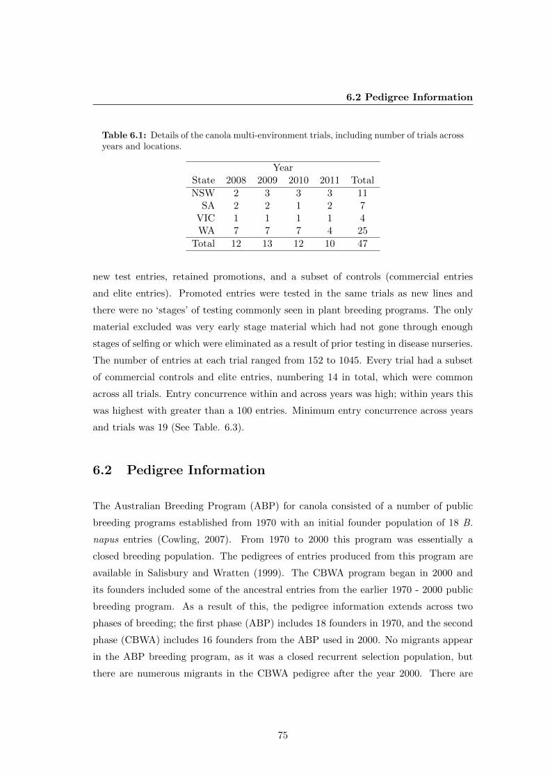
6.2 Pedigree Information
Table 6.1: Details of the canola multi-environment trials, including number of trials acrossyears and locations.
YearState 2008 2009 2010 2011 Total
NSW 2 3 3 3 11SA 2 2 1 2 7
VIC 1 1 1 1 4WA 7 7 7 4 25
Total 12 13 12 10 47
new test entries, retained promotions, and a subset of controls (commercial entries
and elite entries). Promoted entries were tested in the same trials as new lines and
there were no ‘stages’ of testing commonly seen in plant breeding programs. The only
material excluded was very early stage material which had not gone through enough
stages of selfing or which were eliminated as a result of prior testing in disease nurseries.
The number of entries at each trial ranged from 152 to 1045. Every trial had a subset
of commercial controls and elite entries, numbering 14 in total, which were common
across all trials. Entry concurrence within and across years was high; within years this
was highest with greater than a 100 entries. Minimum entry concurrence across years
and trials was 19 (See Table. 6.3).
6.2 Pedigree Information
The Australian Breeding Program (ABP) for canola consisted of a number of public
breeding programs established from 1970 with an initial founder population of 18 B.
napus entries (Cowling, 2007). From 1970 to 2000 this program was essentially a
closed breeding population. The pedigrees of entries produced from this program are
available in Salisbury and Wratten (1999). The CBWA program began in 2000 and
its founders included some of the ancestral entries from the earlier 1970 - 2000 public
breeding program. As a result of this, the pedigree information extends across two
phases of breeding; the first phase (ABP) includes 18 founders in 1970, and the second
phase (CBWA) includes 16 founders from the ABP used in 2000. No migrants appear
in the ABP breeding program, as it was a closed recurrent selection population, but
there are numerous migrants in the CBWA pedigree after the year 2000. There are
75

6. CANOLA MULTI-ENVIRONMENT TRIAL DATA SET
Table 6.2: Summary of individual trial details from the canola multi-environment trials,including total number of entries, replication levels, number of columns, rows, trial meanyield (t/ha), as well as missing yield and pedigree entries.
entries Columns Rows Trial Missing ValuesTrial Total r = 1 r = 2 r > 2 Mean Yield Yield Pedigree
CIA08ARDL2 153 55 93 5 6 43 1.31 1 5CIA08BUN6 152 55 93 4 6 43 1.90 0 6CIA08ELM3 153 55 93 5 6 43 0.27 14 5CIA08HOR3 153 55 94 4 6 43 0.90 0 5CIA08KEL6 152 55 92 5 6 43 1.14 0 7CIA08KOJ6 153 55 94 4 6 43 1.53 9 5CIA08MIN6 152 55 92 5 6 43 2.46 0 7CIA08NYA6 152 55 91 6 6 43 1.37 1 6CIA08PLI5 153 55 94 4 6 43 0.88 0 5
CIA08SCA6 153 55 94 4 6 43 0.94 0 5CIA08WAGG2 153 55 94 4 6 43 0.59 0 5
CIA08YOR6 153 55 95 3 6 43 1.64 0 5CIA09ARDL2 320 257 62 1 12 32 0.26 0 6
CIA09BUN6 304 247 55 2 12 32 0.99 24 6CIA09CCRK2 320 257 62 1 12 32 1.46 1 6
CIA09ELM3 321 258 63 0 12 32 0.58 6 6CIA09HOR3 320 257 62 1 12 32 1.52 0 6CIA09KEL6 321 258 63 0 12 32 1.09 0 6CIA09KOJ6 320 257 62 1 12 32 2.21 0 6CIA09MIN6 321 258 63 0 12 32 1.45 2 6CIA09NYA6 321 258 63 0 12 32 0.54 3 6CIA09PLI5 321 258 63 0 12 32 1.14 0 6
CIA09SCA6 320 257 62 1 12 32 0.55 1 6CIA09WAGG2 320 257 62 1 12 32 2.92 0 6
CIA09YOR6 716 653 62 1 12 65 1.80 2 6CIA10ALBR2 393 320 55 18 12 41 2.54 0 14CIA10ARDL2 394 319 58 17 12 41 1.93 0 13
CIA10BUN6 390 318 53 19 12 41 0.95 0 14CIA10CCRK2 395 322 62 11 12 41 1.47 2 12
CIA10ELM3 391 316 59 16 12 41 1.48 1 13CIA10KEL6 394 319 64 11 12 41 0.30 0 12CIA10KOJ6 394 321 57 16 12 41 1.30 0 13CIA10MIN6 393 318 61 14 12 41 0.59 2 12CIA10NYA6 399 325 62 12 12 41 0.30 0 12CIA10PLI5 395 323 57 15 12 41 1.67 1 13
CIA10SCA6 395 322 56 17 12 41 0.81 4 13CIA10YOR6 970 891 64 15 12 91 1.06 6 12
CTTA11ALBR2 426 349 72 5 12 44 1.47 4 53CTTA11BUNT6 354 242 89 23 12 44 1.49 2 56CTTA11CCRK2 423 348 69 6 12 44 2.03 0 59CTTA11ELMR3 424 346 72 6 12 44 2.15 0 53CTTA11LKBL3 419 340 73 6 12 44 0.96 12 57
CTTA11MNGN6 371 260 92 19 12 44 1.91 3 52CTTA11PTLI5 423 347 70 6 12 44 0.65 4 60CTTA11SSTL6 425 347 72 6 12 44 0.86 0 54
CTTA11WAGG2 423 346 71 6 12 44 0.95 3 57CTTA11YORK6 1045 945 91 9 12 99 1.31 0 61
76

6.2 Pedigree Information
Table 6.3: Entry commonality (concurrence) across trials within years in the canola multi-environment trials data set for the 2008 to 2011 growing seasons. Diagonal values indicatethe total number of entries at the sites within a year.
Year 2008 2009 2010 2011
2008 153 58 21 222009 58 717 113 622010 21 113 970 1022011 22 62 102 1084
up to 16 generations of pedigree information from 1970 to 2011 (Table 6.4). Pedigree
information has been used in CBWA MET analysis of yield and oil traits using the
method of Oakey et al. (2007) from 2008 onwards.
For the MET data set the pedigree information went back several generations to the
1970 founders (Table 6.4). Pedigree information was available for a total of 3208 entries
across the breeding program, with 22 entries having unknown pedigrees. In this case,
unknown pedigrees meant that they were either unknown filler entries or commercial
entries of other companies, for which pedigree information was not available. For
the complete MET data set, there were 146 unique mother entries and 700 unique
father entries. The same entry can be used as a male and/or female parent in a
cross due to canola being a self - pollinated crop. Hence there are multiple instances
of parental concurrence across the pedigree data set across and within years. The
maximum concurrence for parents (both male and female) between years was 169 (2010
and 2011) and the minimum concurrence for parents between years was 43 (2008 and
2010). Within a year the minimum number of parents was 92 and the maximum was
416 across the 4 year data set (Table 6.5).
The entries included in this data set resulted from a wide range of breeding methods,
including F1 hybrids, doubled haploidy (DH), single seed descent (SSD) and synthetic
entries (a type of composite derived from multiple entires). Hence there were various
levels of self-fertilization, that needed to be accommodated when forming the additive
genetic relationship matrix (A matrix). The A matrix in ASReml-R (Butler et al.,
2009) is calculated from information on genetic relationships supplied in a ‘Pedigree
file’. This file comprises four fields of information: Identity of the entry, Male parent,
Female parent and Fgen (see Table 6.6). Self-fertilization or inbreeding is quantified
77

6. CANOLA MULTI-ENVIRONMENT TRIAL DATA SET
Table 6.4: Number of generations of pedigree information available for entries in thecanola multi-environment trials data set.
Generations of No. ofPedigree entries
0 21871 6612 1003 884 435 176 157 128 149 1310 911 612 813 1114 915 1016 5
Table 6.5: Concurrence of parents (both male and female) across trials within years in thecanola multi-environment trials data set for the 2008 to 2011 growing seasons. Diagonalvalues indicate the total number of parents at all sites within a year.
Year 2008 2009 2010 2011
2008 92 54 43 552009 54 395 106 1392010 43 106 416 1692011 55 139 169 291
under the variable Fgen in this file. The pedigree file is also sorted to ensure that the
line of an entries’ pedigree will always precede any line where it appears as a parent.
In the CBWA data set values for Fgen are calculated from the last generation of single
plant selection when using pedigree selection methods. For competitor entries, Fgen
values were based on records obtained from Plant Breeders Right’s (PBR) data base
(http://www.ipaustralia.gov.au/), where available. In the special case of composite
varieties, Fgen values were derived from calculations outlined by Busbice (1969). Fgen
values varied from 0 corresponding to F1 hybrids and back cross intermediates, 0.74 to
0.9 (inbreeding values) for synthetic or composite entries, 1 to 5 (generations of selfing)
for pedigree entries, and a standard of 3 or 4 for SSD, and 10 corresponding to DH
populations (Table 6.7).
78

6.2 Pedigree Information
Table 6.6: Example extract of the CBWA Pedigree file indicating entry, parents andFgen fields of information. Note that “0”’ represents no parent information, normally forfounder parents.
Entry Female Parent Male Parent FgenZephyr 0 0 4.00
Bronowski 0 0 4.00SV62-371 0 0 4.00
Ramses 0 0 4.00Oro 0 0 4.00
Haya 0 0 4.00Zephyr/Bronowski Zephyr Bronowski 4.00
Chisaya 0 0 4.00ATR-Tower 0 0 4.00
Norin20 0 0 4.00Chikuzen 0 0 4.00
SV62-371/Zephyr SV62-371 Zephyr 4.00BJ42 0 0 4.00
Wesway Ramses Oro 3.00
Inbreeding coefficients for entries in the pedigree were calculated using the A.inverse
function in ASReml-R, which uses the algorithm of Meuwissen and Luo (1992) with
adjustments for selfing. These inbreeding coefficients ranged from 0 (477 entries) to
> 0.99 (1797 entries) with an average of 0.68.
Table 6.7: Summary of entry details within the canola multi-environment trials, includingnumber of selfing cycles (Fgen) and their corresponding entry type.
Fgen Levels Entry Type Number of entries
0 Backcross derived, Hybrids 10830.74 Synthetic 20.9 Composite or Synthetic entries 11
0.932 F2 derived composite 10.941 F2 derived composite 1
1,2,3,4,5,6,7 Selections, Breeding entries 1353,4 SSD entries 581
5 Canola Breeders migrants 8210 DH entries 1312
Using the package ‘Pedicure’ (Butler, 2012) in R, a set of 12 pedigree files of varying
depth (in terms of generations) were generated for 4 data sets of varying length (in
terms of years of trial data) (Table 6.8). In the MET data set, the most recent data
was for the 2011 growing season so all combinations of years included 2011 with the
addition of an extra year to a maximum of 4 years of data. The minimum depth of
pedigree was 2 generations, that is the pedigree comprised parents of entries within the
data set.
79

6. CANOLA MULTI-ENVIRONMENT TRIAL DATA SET
As more pedigree information was added (as the depth of pedigree increased), the
number of new parents added to the ancestry decreased with each additional generation.
While there was pedigree information for 16 generations, additional parents were no
longer added after the 13th generation. Hence, the pedigree files were limited to that
generation. Within the generated pedigree files, there were 2 possible levels of founder
populations, up to 9 generations; which consists of the CBWA founders and up to 13
generations which includes the ABP founders (Table 6.8).
Table 6.8: The number of parents (and then grandparents) in the pedigree for varyinggeneration depth and years of data for current entries in the multi-environment trial dataset. The number in the brackets indicates the number of additional parents (and thengrandparents) that result with inclusion of an additional generation of pedigree information.
Length of data set (years of data)No. 2011 2010-2011 2009-2011 2008-2011
Generations
2 1417a 2499 3054 30843 1462b (45) 2549 (50) 3111 (57) 3139 (55)4 1484 (22) 2573 (24) 3131 (20) 3157 (18)5 1498 (14) 2585 (12) 3143 (12) 3169 (12)6 1507 (9) 2594 (9) 3152 (9) 3182 (13)7 1521 (14) 2608 (14) 3166 (14) 3193 (11)8 1527 (6) 2614 (6) 3172 (6) 3198 (5)9 1530 (3) 2617 (3) 3175 (3) 3201 (3)
10 1534 (4) 2621 (4) 3179 (4) 3203 (2)11 1542 (8) 2625 (4) 3183 (4) 3206 (3)12 1542 (0) 2629 (4) 3187 (4) 3208 (2)13 1544 (2) 2631 (2) 3189 (2) 3210 (2)
a For a single year of data this cell indicates that there are 1417 parents for the entries in 2generations of pedigree data, i.e 2 generations consists of entries and their parents.b For a single year of data this cell indicates that there are 1462 parents and grandparents for the
entries in 3 generations of pedigree data, i.e 3 generations consists of entries, their parents and their
grandparents.
80

Chapter 7
Spatial analysis (N-gen
modelling) of trials with pedigree
information
This chapter illustrates in detail the spatial analysis (or non-genetic, ‘Ngen’ modeling)
of the 2011 growing season trials, described in Chapter 6. The impact of including
pedigree information is also evaluated on the spatial mixed model analysis of plant
breeding trials. These spatial models are then used in Chapter 8 for a complete MET
analysis.
7.1 Introduction
Plant breeding programs utilize extensive METs across locations and years (synony-
mous with seasons) to select test entries for promotion, commercialization and use
as parents. Such data from field trials exhibit spatial variation, which arises from the
physical location of plots within a field (Smith et al., 2002a). Thus spatial variation can
be defined as the variable growing conditions encountered throughout a trial (Stringer
et al., 2011). If not accounted for, the presence of extraneous variation can complicate
the analysis, as well as reduce the efficiency of selection (Stefanova et al., 2009). In
81

7. SPATIAL ANALYSIS (N-GEN MODELLING) OF TRIALS WITHPEDIGREE INFORMATION
order to control error in field trials, spatial models are often included within the mixed
model framework.
Gilmour et al. (1997) developed an analysis, which encompasses the modeling of
spatial variation within a mixed model context. This approach for spatial analysis
accommodates three sources of variation, namely global, local and extraneous. Global
trend refers to variation that occurs across the field, local represents short-term trend
such as soil fertility and extraneous variation is the result of experimental procedures
that are aligned with rows and columns (Gilmour et al., 1997). Local trend is accom-
modated within the mixed model by an appropriate covariance structure of which the
separable autoregressive process of order 1 (denoted AR1×AR1) is the most commonly
used (Smith et al., 2002b). This effectively reflects the observation that plots, which
are closer together are more likely to be similar to ones that are further apart (Smith
et al., 2002b). Global trend and extraneous variation however are accommodated by
including additional design factors and random row/column components.
Spatial analysis has been applied to designed field experiments, for both agriculture
(Cullis et al., 1998, 2006, Gilmour et al., 1997) and forestry experiments (Dutkowski
et al., 2006) to correct for environmental effects. This approach has been demonstrated
to result in greater accuracy and precision for the estimation of treatment effects (Cullis
et al., 1998, Smith et al., 2001b,a) and thus leads to large reductions in effective er-
ror variance (Smith et al., 2006). However, the value of spatial analysis is especially
demonstrated in improving the reliability of varietal selection when trials are large and
have minimal replicates (Smith et al., 2001a, Stefanova et al., 2009). This is especially
the case with a class of designs commonly used in plant breeding programs called ‘repli-
cated plots for a percentage (p) of the test lines’, or p-rep designs (Cullis et al., 2006).
P-rep trial designs are often used for the testing of early generation entries. These de-
signs are useful as they are based on optimal spatial relationships, enable unbalanced
replication in check entries and test entries, to account for availability of seed, and
allows test entries to be the focus of the design (Cullis et al., 2006).
Since Gilmour et al. (1997) demonstrated the need to identify the sources and causes
of spatial variation within a mixed model framework of analysis, it has become a stan-
dard component for numerous plant breeding based studies (Cullis et al., 2006, Smith
82

7.2 Methods and Materials
et al., 2002a, Oakey et al., 2006, 2007, Kelly et al., 2007). Stefanova et al. (2009)
has since extended this process by including advanced diagnostics for the selection of
non-genetic variance models, with the aim of reducing the ambiguity in choosing ap-
propriate spatial models. However there are some instances where spatial models have
not been included when pedigree information is used in mixed model analysis. For
example Crossa et al. (2006) and Burgueno et al. (2007) modeled additive (A) and
additive by additive (AxA) effects respectively in CIMMYT international wheat trials,
with the omission of spatial models. Due to the absence of design components and
spatial correlation in these studies, the study by Beeck et al. (2010) considered that
these models were ‘simplistic models for non-genetic effects’.
In Chapter 5, it was highlighted that the selection of non-genetic variance models are
a source of complexity hindering the more widespread use of mixed model analysis with
pedigree information. This was also highlighted in the paper by Beeck et al. (2010),
where the authors state that such model identification it is a component of difficulty
for the analysis of MET data sets. This chapter addresses this by demonstrating the
process of non-genetic variance modeling for an actual plant breeding data set, coded
for anonymity. This process also aims at evaluating the differences that may arise in
the spatial analysis of plant breeding METs from the inclusion of pedigree information.
This chapter commences with a brief description of the CBWA data set, before under-
taking a series of analyses contrasting standard and pedigree models at a single trial
level. The findings of the spatial modeling with pedigree are then discussed within the
context of the breeding data.
7.2 Methods and Materials
7.2.1 Data set description
The data set for this chapter consists of the 2011 subset of the full CBWA MET yield
data described in Chapter 6. Briefly, the 2011 data set comprised 10 trials with a total
of 1084 varieties tested across locations (Table 7.1). Trials were individually designed
using a p−rep design (Cullis et al., 2006) with a ‘superblock’ (see Section 7.2.1.1 for
details) component with a majority of varieties sown once or with an extra replicate.
83
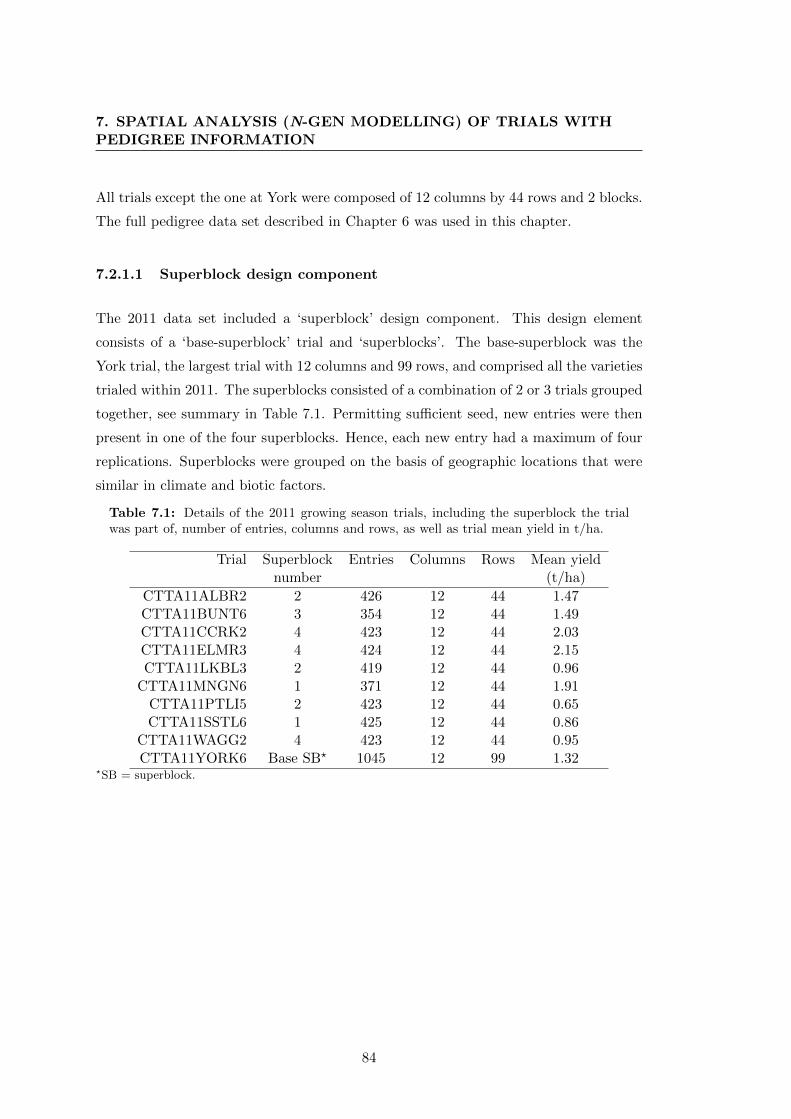
7. SPATIAL ANALYSIS (N-GEN MODELLING) OF TRIALS WITHPEDIGREE INFORMATION
All trials except the one at York were composed of 12 columns by 44 rows and 2 blocks.
The full pedigree data set described in Chapter 6 was used in this chapter.
7.2.1.1 Superblock design component
The 2011 data set included a ‘superblock’ design component. This design element
consists of a ‘base-superblock’ trial and ‘superblocks’. The base-superblock was the
York trial, the largest trial with 12 columns and 99 rows, and comprised all the varieties
trialed within 2011. The superblocks consisted of a combination of 2 or 3 trials grouped
together, see summary in Table 7.1. Permitting sufficient seed, new entries were then
present in one of the four superblocks. Hence, each new entry had a maximum of four
replications. Superblocks were grouped on the basis of geographic locations that were
similar in climate and biotic factors.
Table 7.1: Details of the 2011 growing season trials, including the superblock the trialwas part of, number of entries, columns and rows, as well as trial mean yield in t/ha.
Trial Superblock Entries Columns Rows Mean yieldnumber (t/ha)
CTTA11ALBR2 2 426 12 44 1.47CTTA11BUNT6 3 354 12 44 1.49CTTA11CCRK2 4 423 12 44 2.03CTTA11ELMR3 4 424 12 44 2.15CTTA11LKBL3 2 419 12 44 0.96
CTTA11MNGN6 1 371 12 44 1.91CTTA11PTLI5 2 423 12 44 0.65CTTA11SSTL6 1 425 12 44 0.86
CTTA11WAGG2 4 423 12 44 0.95CTTA11YORK6 Base SB? 1045 12 99 1.32
?SB = superblock.
84
7.2 Methods and Materials
7.2.2 Single Trial analysis
Beeck et al. (2010) set out a process for mixed model selection, which consists of
two components, the first being the selection of the model for the genetic variance
structure and the second being the variance models for the trial non-genetic effects
(which they refer to as Ngen-variance models). At a single trial, a description of the
Ngen modeling with genetic models which exclude and include pedigree information
is first outlined. Following the process of Oakey et al. (2006, 2007) the models which
exclude pedigree information are referred to as Standard models and those which include
pedigree information are referred to as Pedigree models.
7.2.2.1 Standard statistical model
A single trial analysis without pedigree information for the jth (j = 1, ...., t) trial in the
CBWA data set is first described. Each trial is comprised of m entries in a rectangular
array of plots with rj rows and cj columns, so that the number of plots in a trial is
given by nj = rjcj . The spatial mixed model can be written as,
yj = Xjτ j +Zvjuvj +Zpjupj + ej (7.1)
where, yj is an n × 1 vector of entry yields in t/ha, ordered as rows within columns;
τ j is the vector of fixed effects, which in most trials includes an overall trial mean and
any additional trial specific spatial modeling terms, such as linear regression across
row; the associated design matrix is Xj ; uvj is a m× 1 vector of random entry effects,
with associated design matrix Zvj ; upj is a vector of random peripheral effects (non-
genetic), which includes block effects and other spatial modeling terms such as random
row effects; the associated design matrix is Zpj ; ej is the vector of residuals, ordered
as per the data vector.
The variance assumptions for random entry effects are:
var(uvj
)= σ2
vjIm
where σ2vj is the entry variance and Im is an identity matrix of order m.
85

7. SPATIAL ANALYSIS (N-GEN MODELLING) OF TRIALS WITHPEDIGREE INFORMATION
The variance assumptions for random peripheral effects are:
var(upj
)= Gp = ⊕bj
l=1σ2pjlIqjl
where each trial has a maximum of bj random peripheral terms, and the lth term
(l = 1, ..., bj) has qjl effects and an associated variance component of σ2pjl
.
In terms of the errors, an AR1 model was used to model local trend. The AR1 model
has been previously demonstrated as the most commonly used for local spatial trend
(Smith et al., 2002b). Hence for a separable AR1 process for both rows and columns
the variance matrix of errors is:
var (ej) = Rj = σ2jΣcj ⊗Σrj (7.2)
where σ2j is the error variance, and Σcj and Σrj are correlation matrices of dimensions
c× c and r × r of AR1 processes in the column and row directions respectively. Each
matrix is a function of a single autocorrelation parameter ρcj and ρrj for the column
and row dimensions respectively. Given a set of ordered spatial coordinates (row or
column number) the correlation matrix has the form of:
Σ(ρ) =
1 ρ1 ρ2 · · · ρn−1
ρ1 1 ρ1 · · ·...
ρ2 ρ1 1 · · ·...
......
.... . .
...
ρn−1 · · · · · · · · · 1
Thus the models for non-genetic variation encompass model terms for both trial design
and spatial variation.
7.2.2.2 Pedigree statistical model
The mixed model with pedigree information is then fitted. This is an extension of
Equation 7.1 developed by Oakey et al. (2006) for a single trial analysis of a wheat
data set. Under the pedigree model, the model for uv is given by, uv = ua + ui,
that is the vector for random entry effects (uv) is partitioned into additive genetic
effects (ua(m×1)) and non-additive genetic effects (ui
(m×1)). Note that in the pedigree
86
7.2 Methods and Materials
statistical model, m is the number of entries in the pedigree. Thus the mixed model
for the jth (j = 1, ......, t) trial in the motivational data set can be written as,
yj = Xjτ j +Zvj(uaj + uij) +Zpjupj + ej (7.3)
The equation terms and the variance assumptions are as stated above for the standard
model. The variance assumptions for the additive and non-genetic effects are,
var (ua) = σ2aA
var (ui) = σ2i Im
Where the matrix A(m×1) = {aij} is the additive genetic relationship matrix which has
elements,
aii = 1 + Fi
aij = 2fij
where Fi is the inbreeding coefficient of entry i and fij is the coefficient of parentage
between entries i and j. Note that the total genetic effect was partitioned into additive
and non-additive effects, as the data set had a high level of inbreeding (1797 entries
had inbreeding coefficients of > 0.99).
7.2.3 Ngen variance modeling
This component involved choosing an appropriate model for the non-genetic effects,
through the use of graphical diagnostics. For each trial, the standard model was first
fitted and diagnostics used to determine if additional Ngen parameters were required
to accommodate global trend/extraneous variation and to check the adequacy of the
variance structure of local trend.
Diagnostics for Ngen examination, included the 3D sample variogram and plot of
residuals against row/column numbers (termed as residual plots) from Gilmour et al.
(1997) and the sample variogram augmented with coverage intervals obtained from
simulations from Stefanova et al. (2009). This latter approach was based on an approach
by Atkinson (1985), who used simulation to provide a reference for a set of fluctuations.
87

7. SPATIAL ANALYSIS (N-GEN MODELLING) OF TRIALS WITHPEDIGREE INFORMATION
In Stefanova et al. (2009) this application consisted of plots of the ‘faces’ of the sample
variograms corresponding to zero row displacement (referred to as the column face)
and zero column displacement (referred to as a row face), which were plotted alongside
approximate 95% point-wise coverage intervals obtained from parametric bootstrap
simulations of the current model. The coverage intervals presented in this chapter were
based on N = 100 simulations.
7.2.4 Outlier detection
Erroneous data points were excluded based on formal tests of significance for outliers
in spatial analysis using the Alternative Outlier Mixed Model (AOMM) in ASReml-R
(Smith et al. unpublished). This process produces Studentised conditional residuals
(Scres) as part of the outlier identification diagnostics. For each trial, these Scres
from the pedigree model were plotted against those obtained from the standard model.
While AOMM diagnostics were used as a formal method of outlier identification, the
plant breeder was still consulted to determine which points were erroneous.
7.2.5 Analysis
For each of the trials, the Standard and Pedigree models were first fitted (these were
termed ‘base’ as they did not include any extraneous variation terms) followed by
AOMM diagnostics. Ngen diagnostics from both the base models were then used to
determine if additional global trend or extraneous variation terms were added. If this
was the case, Ngen diagnostics were repeated after each of the terms were added to
the model. Such stages of Ngen diagnostics enabled a comparison between spatial
covariance structures under the different models. A detailed description of Ngen model
fitting is first provided for the CTTA11YORK6 trial and then summarized for all other
trials. Note that for the sake brevity in this chapter and the next, the trial prefix
‘CTTA11’ will be dropped when reporting in the results and discussion. Trials will
instead be referred to by their location acronym and state number, i.e CTTA11YORK6
will now be referred to as YORK6.
88

7.3 Results
7.2.6 Estimation and Fitting
The estimation and fitting of the models are as previously described in Chapter 3. For
the pedigree models, the A−1 matrix was computed in R (R Development Core Team,
2012) package ASReml-R (Butler et al., 2009) using the A.inverse function, which uses
the algorithm of Meuwissen and Luo (1992) with adjustments for selfing.
7.3 Results
7.3.1 Ngen variance modeling - York trial
This section illustrates the N-gen modeling process for standard and pedigree models for
the York trial in detail. An overview of the series of Ngen models fitted are summarized
in Table 7.2.
Plots of residuals and sample variograms corresponding to the base model can be
seen for the standard model in Fig. 7.1a and for the pedigree model in Fig. 7.1b
respectively. For both these models, the corresponding variograms indicate the presence
of a strong linear trend, as both the sample variograms fail to reach a plateau as
expected in the theoretical sample variogram. This is also seen in both the residual
plots with a linear trend over row number for each column. These linear row effects
are also reflected by observing the row faces of both models, standard (Fig. 7.2c ) and
pedigree (Fig. 7.2d), of the augmented sample variogram. For both these row faces, the
sample variogram increases with increasing row separation exceeding the upper 95%
coverage interval before decreasing rapidly to below the mean of the simulations.
Model 1a and 2a (Table 7.2), which included a linear regression across rows for the
standard and pedigree models, were then fitted. The resulting sample variograms can
be seen in Fig. 7.3. The linear increase in residuals across rows for columns is no
longer observed. The presence of local spatial variation is seen by the smooth trend of
the residual plot. However, it is evident that there are random column effects, seen by
the jagged pattern in the column dimension of the sample variogram. The row face of
the augmented sample variograms is reviewed to confirm this. For both models, the
corresponding row faces of the augmented sample variograms (Fig. 7.4c and Fig. 7.4d),
89

7. SPATIAL ANALYSIS (N-GEN MODELLING) OF TRIALS WITHPEDIGREE INFORMATION
indicates that the previous steep increase in the sample variogram is no longer seen,
instead a plateau is reached. However both sample variograms are also well below the
mean of the simulations and the sills are actually outside the coverage interval, indica-
tive of random column effects. The sample variogram for the pedigree model however,
appeared to be well below the lower confidence interval while the sample variogram
for the standard model was in-between the mean of the simulations and the bottom
confidence interval. Hence it was more obvious that the inclusion of column effects was
required under the pedigree model. The sample variogram from the column face of
the standard model (Fig. 7.4a) follows the mean of the simulations quite closely, and
no longer exceeds the upper or lower 95% confidence intervals. The sample variogram
from the column face of the pedigree model however, still exceeds the lower confidence
interval at around the 5th column displacement(Fig. 7.4b).
Models 1b and 2b (Table 7.2) were then fitted which included random column effects.
There is a large increase in REML log likelihood in comparison to the corresponding
previous models (Table 7.2). The resulting sample variograms can be seen in Fig, 7.5.
For the standard model, the smooth local trend observed previously (Fig. 7.3) is no
longer seen (ρr = 0.27 compared to ρr = 0.91, Table 7.2) however smooth local trend
is still evident for the pedigree model (ρr = 0.58, compared to ρr = 0.90, Table 7.2).
The augmented sample variograms (Fig. 7.6) both indicate that standard and pedi-
gree models show good agreement with the mean of the simulations and lie between
the 95% coverage intervals.
90
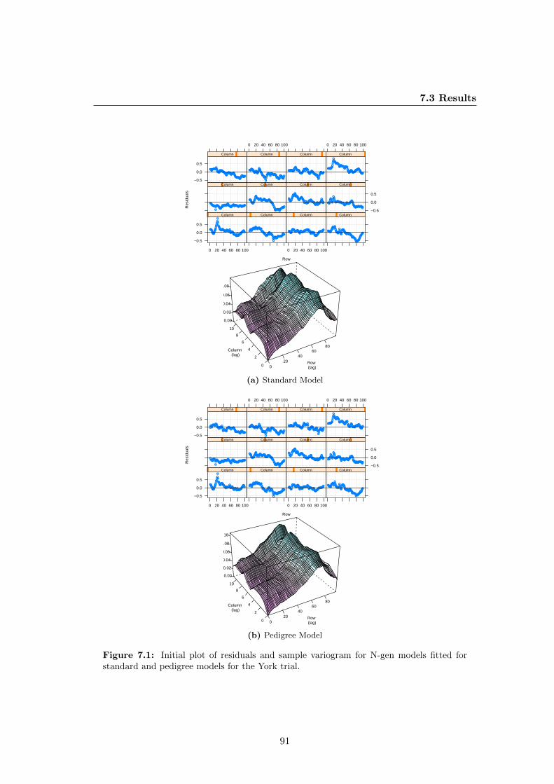
7.3 Results
york11.asr1
Row
Res
idua
ls
−0.5
0.0
0.5
0 20 40 60 80 100
●●●●●●●●●●●
●●●●●●●●●●
●
●
●●●●●●●●●●●●
●●●●●●●●●●●●●●●●●●●
●●●●●●
●●●●●●●●●●●●●●●●●●●●●●
●●●●●●●●●
●●●●●●
Column
●●●●●●●
●●●●●●●●●●
●●●●●●●●●●●●●●●●
●●●●●●●●●●●●●●●●●●●●●●●●●●●●●●●●
●●●●●●●●●●●●●
●●●●●●●●●●●●●●●●●●●●
Column
0 20 40 60 80 100
●●●●●●●●●●●●●●●●●●●●●●●●
●●●●●●●●●●●●●●●●●●●
●●●●●●●
●●●●●●●●
●●●●●●●●●
●●●●●●●●●●●
●●●●●●●●●●●●●
●●●●
Column
●●●●●●●●●●●●●●●●●
●●●●●●●●●●●●●
●
●●●●●●●●●●●●●●●
●●●●●●●●●●●●●●●●●●●●●●●●●●●●●●
●●●●●●●●●●●●●●●●●●●●
Column
●●●●●●●●●●●●●●
●
●●●●●●●●●●●●●●●
●●●●●●●●●●●●
●●●●●●●●●●●●●●●●●●●
●●●●●●●●●
●●●●●●●●●●●●●●●●●●●●●●●●●
●●●
Column
●●●●●●●●●●●●
●●●●●●●●●●●●●●●●●●●
●●●●●●●●●
●●●●●●●●●●●●●●●●●●●●●●●●●●
●●●●●●●●●●●
●●●●●●●●●●●●●
●●●●●●●
Column
●●●●●●●
●●●●●●●●●●●●●●●●●●
●●●●●●●●●
●●●●●●●●●●●●●●●●●●●
●●●●●●●
●●●●●●●●●●●●●●●●●●●●●●●●●●●
●●●●●●●●●●
Column
−0.5
0.0
0.5
●●●●●●●●●●●●●●●●●●●●●●●●●●
●●●●●●●●●●●●●●●●●●●●●●●●●●●●●●●●●●●
●●●●●●●●
●●●●●●●●●●●●●●●●●●●●●●●●●●●●
Column−0.5
0.0
0.5●●●●●●
●●●●●●●●●●●●●●●●●●●●●
●●●●●●●●●●●●●●●●●
●●●●●●●
●●●●●●●●●●●●●●●●●
●●●●●●●●●●●●●●●●
●●●●●●●●●●●●●
Column
0 20 40 60 80 100
●●●●●●●●●●●●●●●●●
●●●●●●●●●●●●●●
●●●●●●●●●●●●●●
●●●●●●●●●●●●●●
●●●●●●●●●●●●●●●●●
●●●●●●●●●●
●●●●●●●●●●●
●●
Column
●●●●●●●●●●●●●●●●●●●●●●●●●●●●●●●
●●●●●●●●●●●●●●●●
●●●●●●●
●●●●●●●●●●●●●●●●●●●●●●●●●●
●●●●●●●●●●●●●●●●●●
Column
0 20 40 60 80 100
●●●●●●●●●●●●●●●●●●●●●●●●●●●●●
●●●●●●●●●●●●●●
●●●●●●●●●
●●●●●●●●
●●●●●●●●●●●●●●●●●●●●●●
●●●●●●●●●●●●●●
Column
020
4060
80
0
2
4
6
8
10
0.00
0.02
0.04
0.06
0.08
Row (lag)
Column (lag)
(a) Standard Modelyork11.asr2
Row
Res
idua
ls
−0.5
0.0
0.5
0 20 40 60 80 100
●●●●●●●●●●●
●●●●●●●●●●
●
●
●●●●●●●●●
●●●●●●●●●●●●●●
●●●●●●●●●●●●●●
●●●●●●●●●●●●●●●●
●●●●●●●●●
●●●●●●●●●●●●
Column
●●●●●●●●●●●●●●●●●
●●●●●●●●●●●●●●●●●●●●●●●●●
●●●●●●●●●●●●●●
●●●●●●●●●
●●●●●●●●●●●●●●
●●●●●●●●●●●●●●
●●●●●
Column
0 20 40 60 80 100
●●●●●●●●●●●●●●●●●
●●●●●●●●●●●●●
●●●●●●●●●
●●●●●●●●●●●
●●●●●●●●
●●●●●●●●●●●●●●●●●●●
●●●●●●●●●●
●●●●●●●●
Column
●●●●●●●●●●●●●●●
●●●●●●●●●●●●●●●●
●●●●●●●●●●●●●
●●●●●●●●●
●●●●●●●●●●●●●
●●●●●●●●●●●●●●●
●●●●●●●●●●●
●●●●
Column
●●●●●●●
●●●●●●●
●
●●●●●●●●●●●●●●●
●●●●●●●●●●●●●●●●●●
●●●●●●●●●●●●●●●●●●●
●●●●●●●●●●●●●●●●●●●●●●●●
●●●●●●●
Column
●●●●●●●●●●●●●
●●●●●●●●●●●●●●●
●●●●●●●●●●●●●●●●●
●●●●●●●●●●●●●●●●●●●●●●●
●●●●●●●●●
●●●●●●●●●●●●●
●●●●●●●
Column
●●●●●●●
●●●●●●●
●●●●●●●●●●●●●●●●●●
●●●●●●●●●●●●●●●●●●●●●●
●●●●●●●●●
●●●●●●●●●●●●●●●●●●●●●●
●●●●●●●●●●●●
Column
−0.5
0.0
0.5
●●●●●
●●●●●●●●
●
●●●●●●●●●●●●
●●●●●●●●●●●●●●●●●●●●●●●
●●●●●●●●●●●●●●●●●●●●
●●●●●●●●●●●●●●●●●●●●●●●●●●●●
Column−0.5
0.0
0.5
●●●●●
●●●●●●●●●●●●●●●
●●●●●●●●●●●●●
●●●●●●●●●●●●●
●●●●●●●●●●●●●●●
●●●●●●●●●●●●●●●●●●●●●●●●
●●●●●●●●●●●●
Column
0 20 40 60 80 100
●●●●●●●●●●●●●●●
●●●●●●●●●
●●●●●●●●●●●●
●●●●●●●●●●●
●●●●●●●●
●●●●●●●●●●●●●●●●●●●●●
●●●●●●●●●●●●●●●●●●●●●
●●
Column
●●●●●●●●●●●●●●●●●●●●●●●●●●●●●●●
●●●●●●●●●●●●●●●●●●●●●
●●
●●●●●●●
●●●●●●●
●●●●●●●●●●●●●●●
●●●●●●●●●●●●●
●●
Column
0 20 40 60 80 100
●●●●●●●●●●●●●●●
●●●●●●●●●
●●●●●●●●●●●●●
●●●●●●●●
●●●●●●●
●●●●●●●●●
●●●●●●●●●●●●●
●●●●●●●●●●●●●●●●●●●
●●●
Column
020
4060
80
0
2
4
6
8
10
0.00
0.02
0.04
0.06
0.08
0.10
Row (lag)
Column (lag)
(b) Pedigree Model
Figure 7.1: Initial plot of residuals and sample variogram for N-gen models fitted forstandard and pedigree models for the York trial.
91

7. SPATIAL ANALYSIS (N-GEN MODELLING) OF TRIALS WITHPEDIGREE INFORMATION
xvar
gam
ma
0.02
0.04
0.06
0.08
0 2 4 6 8 10
(a) Column Face - Standard Modelxvar
gam
ma
0.02
0.04
0.06
0.08
0.10
0 2 4 6 8 10
(b) Column Face - Pedigree Model
xvar
gam
ma
0.02
0.04
0.06
0.08
0 20 40 60 80 100
(c) Row Face - Standard Modelxvar
gam
ma
0.02
0.04
0.06
0.08
0 20 40 60 80 100
(d) Row Face - Pedigree Model
Figure 7.2: Initial plots of faces of the sample variogram (solid line) and the simulationmean (dotted line) as banded by 95% coverage intervals (dashed lines) for standard andpedigree models at the York trial.
92

7.3 Results
york11.asr1a
Row
Res
idua
ls
−0.5
0.0
0.5
0 20 40 60 80 100
●●●●●●●●●●●●●●●●●●●●●
●
●
●●●●●●●●●●●●
●●●●●●●●●●●●●●●●●●●
●●●●●●
●●●●●●●●●●●●●●●●●●●●●
●●●●●●●●●●●●●●●●
Column
●●●●●●●
●●●●●●●●●●
●●●●●●
●●●●●●●●●●
●●●●●●●●●●●●●●●●
●●●●●●●●●●●●●●●●
●●●●●●●●●●●●●
●●●●●●●●●●●●●●●●●●●●
Column
0 20 40 60 80 100
●●●●●●●●●●●●●●●●●
●●●●●●●●●●●●●●●
●●●●●●●●●●
●●●●●●●●
●●●●●●●●●●●●●●●●
●●●●●●●●●●●●●
●●●●●●●●●●●●●
●●●
Column
●●●●●●●●●●●●●●●●●●
●●●●●●●●●●
●●●
●●●●●●●●●●●●●●●
●●●●●●●●●●●●
●●●●●●●●●●●●●●●●●●
●●●●●●●●●●●●●●●●●●●●
Column
●●●●●●●●●●●●●●
●
●●●●●●●●●●●●●●●●
●●●●●●●●●●●●●●●
●●●●●●●●●●●●●●
●●●●●●●●●●
●●●●●●●●●●●●●●●●●●●●●●●●●
●●●
Column
●●●●●●●●●●●●
●●●●●●●●●●●●●●●●
●●●●●●●●●
●●●●●●●●●●●●●●●
●●●●●●●●●●●●●●●●●
●●●●●●●●●●●●●●●●●
●●●●●●●●●●
●
Column
●●●●●●●
●●●●●●●●●●●●●●●●●●●
●●●●●●●●●●●●●●●
●●●●●●●●●●●●
●●●●●●●●●●●●●●●●
●●●●●●●
●●●●●●●●●●●
●●●●●●●●●●
Column
−0.5
0.0
0.5
●●●●●●●●●
●●●●●●●●●●●●●●●●●
●●●●●●●●●●●●●●●●●●●●●
●●●●●●●●●●●
●●●●●●●●●●●
●●●●●●●●●●●●●●●●●●●●●●●●●●
●●
Column−0.5
0.0
0.5
●●●●●●●●●●●●●●●●●
●●●●●●●●●●
●●●●●●●●●●●●●
●●●●●●●●●●●●●●●●
●●●●●●●●
●●●●●●●●●●●●●
●●●●●●●●●●●●●●●●●●
●●
Column
0 20 40 60 80 100
●●●●●●●●●●●●●●
●●●●●●●●●●
●●●●●●●●●●●●
●●●●●●●●●●●
●●●●●●●●●●●●
●●●●●●●●●●●
●●●●●●●●●●●●●●
●●●●●●●●●●●●●
●●
Column
●●●●●●●●●●●●●●●●●●●●●●●●●●●●●●●●●●●●●●●
●●●●●●●●●
●●●●●●
●●●●●●●●●●●●●●●●●●●●●●●●●●
●●●●●●●●●●●●●●●●●●
Column
0 20 40 60 80 100
●●●●●●●●●●●●●●●
●●●●●●●●●●●●●●
●●●●●●●●●●●●●●●●
●●●●●●●
●●●●●●●
●●●●●●
●●●●●●●●●●
●●●●●●●●●●●●●●●●●●●●●
Column
020
4060
80
0
2
4
6
8
10
0.00
0.01
0.02
0.03
0.04
Row (lag)
Column (lag)
(a) Standard Modelyork11.asr2a
Row
Res
idua
ls
−0.5
0.0
0.5
0 20 40 60 80 100
●●●●●●●●●●●
●●●●●●●●●●
●
●
●●●●●●●●●●●●●●●●●
●●●●●●●●●●●●●
●●●●●●●
●●●●●●●●●●●●●●●●
●●●●●●●●
●●●●●●●●●●●●
●
Column
●●●●●●●
●●●●●●●●●●
●●●●●●●●●●●●●●●
●●●●●●●●●●
●●●●●●●●●●●●●●
●●●●●●●●●
●●●●●●●●●●●●●●
●●●●●●●●●●●●●●
●●●●●
Column
0 20 40 60 80 100
●●●●●●●●●●●●●●●●●
●●●●●●●●●●●●●
●●●●●●●●●●
●●●●●●●●●●
●●●●●●●●●●●●●●●●●
●●●●●●●●●
●●●●●●●●●●●●●●●●
●●●
Column
●●●●●●●●●●●●●●●●●●●●●●●●●●●●
●●●
●●●●●●●●●●●●●
●●●●●●●●●
●●●●●●●●●●●●●
●●●●●●●●●●●●●●●●●●●●
●●●●●●
●●●●
Column
●●●●●●●
●●●●●●
●
●
●●●●●●●●●●●●●●●
●●●●●●●●●
●●●●●●●●●●●●●●●●●●●●
●●●●●●
●●●●●●●●●●●●●●●●●●●●●●●●●●
●●●●●●●
Column
●●●●●●●●●●●●●
●●●●●●●●●●●
●●●●●●●●●
●●●●●●●●●●●●
●●●●●●●●●●●●●●●●●●●●●●●
●●●●●●●●●
●●●●●●●●●●●●●
●●●●●●
●
Column
●●●●●●
●●●●●●●●
●●●●●●●●●●●●●●●●●
●●●●●●●●●●●●
●●●●●●●●●●●
●●●●●●●●●
●●●●●●●●●●●●●●●●●●●●●
●●●●●●●●●●●●●
Column
−0.5
0.0
0.5
●●●●●
●●
●●●●●●
●
●●●●●●●●●●
●●●●●●●●●●
●●●●●●●●●●●●●●●
●●●●●●●●●●●●●●●●
●●●●●●●●●●●●●●
●●●●●●●●●●●●●●●●●
●
Column−0.5
0.0
0.5
●●●●●
●●●●●●●●●●
●●●●●●●●●●●●●●●●●●
●●●●●●●●●●●●●
●●●●●●●●●●●●●●●
●●●●●●●●●
●●●●●●●●●●●●●●●●●●●●●●●●●●●
Column
0 20 40 60 80 100
●●●●●●●●●●●●●●●●●
●●●●●●●●●●●●●●●●●●●
●●●●●●●●●●●
●●●●●●●●●
●●●●●●●●●●●●●●●●●●●●●●●●●●●●
●●●●●●●●●●●●●
●●
Column
●●●●●●●●●●●●●●●
●●●●●●●●●●●●●●●●●●●●●●●●
●●●●●●●
●●●●●●●●
●●●●●
●●●●●●●●●●●●●
●●●●●●●●●●●
●●●●●●●●●●●●●
●●
Column
0 20 40 60 80 100
●●●●●●●●●●●●●●●
●●●●●●●●●
●●●●●●●●●●●●●●
●●●●●●●
●●●●●●●
●●●●●●●●●●●●●
●●●●●●●●●●●●●●●
●●●●●●●●●●●●●●●●
Column
020
4060
80
0
2
4
6
8
10
0.00
0.01
0.02
0.03
0.04
Row (lag)
Column (lag)
(b) Pedigree Model
Figure 7.3: Plot of residuals and sample variogram for N-gen models fitted for standardand pedigree models after the addition of linear regression on row number at the Yorktrial.
93
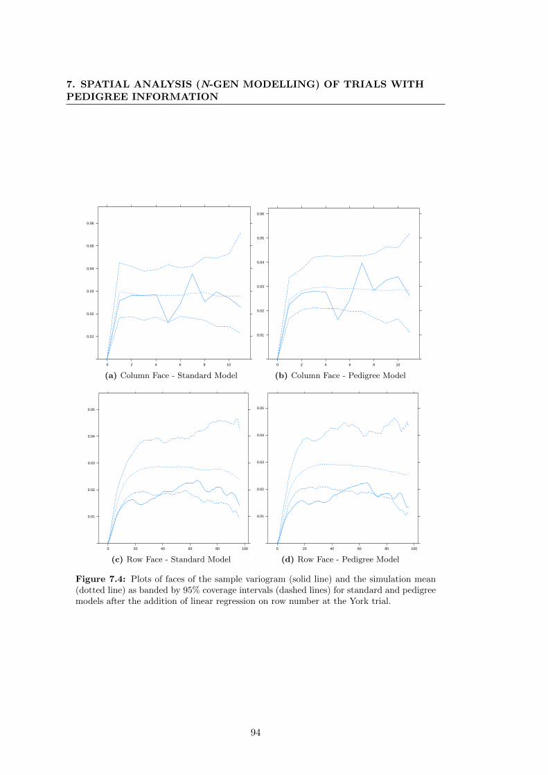
7. SPATIAL ANALYSIS (N-GEN MODELLING) OF TRIALS WITHPEDIGREE INFORMATION
xvar
gam
ma
0.01
0.02
0.03
0.04
0.05
0.06
0 2 4 6 8 10
(a) Column Face - Standard Modelxvar
gam
ma
0.01
0.02
0.03
0.04
0.05
0.06
0 2 4 6 8 10
(b) Column Face - Pedigree Model
xvar
gam
ma
0.01
0.02
0.03
0.04
0.05
0 20 40 60 80 100
(c) Row Face - Standard Modelxvar
gam
ma
0.01
0.02
0.03
0.04
0.05
0 20 40 60 80 100
(d) Row Face - Pedigree Model
Figure 7.4: Plots of faces of the sample variogram (solid line) and the simulation mean(dotted line) as banded by 95% coverage intervals (dashed lines) for standard and pedigreemodels after the addition of linear regression on row number at the York trial.
94
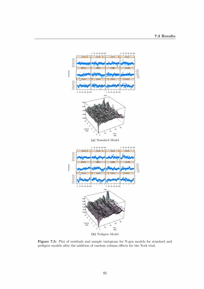
7.3 Results
york11.asr3
Row
Res
idua
ls
−0.4−0.2
0.00.20.40.6
0 20 40 60 80 100
●●●●●●
●
●
●●●
●●●●●●●●
●●
●
●
●●●●
●●
●●
●●●●
●
●●●●
●
●●●●●●
●●●●●●●
●
●
●●●●●
●
●●●●●
●●
●●●●●●
●
●
●●●●●●●●
●●●●●●●
●●●●
●
Column
●●●
●
●●●●●
●●
●
●●●
●●
●●
●●●●
●●●
●●●●●●
●
●●
●●●●
●●●
●●
●●
●●
●●●●●●●
●
●
●●●●●●●●●
●
●
●●●●
●●
●●●●
●●●●
●
●●●●●●●●
●●
●●●●●
Column
0 20 40 60 80 100
●●●●●●
●
●
●●●
●●●●●
●
●
●●●●●●●●●●●●●●●●●●●●
●●●●●●●●
●●●●
●
●●●●
●●●●●●●●●●●●●●●
●●●●●●●●●
●●
●●●●●●●
●●●●
●
●
●
Column
●●●●
●
●●
●
●●●●
●●●●●●
●
●●●●
●
●●●
●
●
●●
●
●●●
●●
●●
●●●●●
●
●
●●●●●●●
●●●
●●●●●
●●●●●
●●
●●●●●●
●●
●
●●●●●●●●●●●●
●
●●●●●●
Column
●●●●●●●●●●
●
●●●
●
●●
●●●●●●●
●●●●●●●●●●
●●
●●●●●●
●●●
●
●●●●●
●●●●●●●●●
●●●
●
●●●
●●
●●●●
●●●●●
●●●●●
●●●●●●
●
●●●●●●●
●
Column
●●●●●
●●●●
●●●●●●●●●
●
●
●
●●●●●
●
●●●●
●
●
●●●
●●●
●
●●●●●●●●●
●●●
●●●●●
●●●●●●●●●
●●●
●●
●●●●●
●
●
●●●●●●
●
●●●●
●●●
●●●●●
Column
●●
●
●
●
●●●
●●●
●
●●
●●
●
●●●
●
●●●●●
●●●●●●●●●●●●●●●●●
●
●
●●
●●●●●●●●●●●●●●
●●●●●
●●●
●●●
●●●
●●●●●
●●●
●●
●
●●●●●●●●
●●●
Column
−0.4−0.20.00.20.40.6
●●●●●●●●●
●
●●●●
●
●●
●●
●●●●●●
●
●●●●●●●●●●●●●●●
●●●●●●●●●●
●
●●●
●●●
●●●
●●
●●
●●●●
●●●●●●
●●●●●●●●●●●●●●●●●●●●
●●
Column−0.4−0.2
0.00.20.40.6
●●●●●●
●●●●●●●●
●
●●
●
●●●●●●
●●●
●●●●●●
●
●●●●●●
●●●●
●●
●●●●
●
●●●●●●
●●●●●●●●●●●
●
●
●●●●●
●
●●●●●
●●●●●
●
●●●●
●●●●
●●
Column
0 20 40 60 80 100
●●●●●
●●●●●●
●●●
●
●●●●●●●●●
●●●
●
●●●
●●●●●
●●●●●●●●
●
●●
●
●●●
●●●●●
●●●
●
●●●●
●●●●●●●●●
●●●●●●●●●●●●●●●●●●●●●●●●●●
Column
●●●●●●●●
●●●●●●●●●●●●●●●●●●●●
●●●●
●●●●●
●●●●●●
●
●●●●
●
●●
●●
●
●
●●●●●●●●●●●
●●●●●●
●●
●●●
●●●
●●●
●●
●●●●
●●●●●●
●●●
Column
0 20 40 60 80 100
●●●●
●
●●
●●●●●●●●
●
●
●
●●●●
●●●●●●
●
●
●
●
●●●●●●●●●●●
●
●
●●●●●●
●
●●●
●
●●●●●●●●●
●●●●
●●●●●●●●●
●●●●●●●●●●●●●●●
●
●
●
Column
020
4060
80
0
2
4
6
8
10
0.000
0.005
0.010
0.015
0.020
Row (lag)
Column (lag)
(a) Standard Modelyork11.asr3a
Row
Res
idua
ls
−0.4−0.2
0.00.20.40.6
0 20 40 60 80 100
●●●●●●●●●●●●●●●●●
●●
●●
●
●
●●●●
●●●●●●●●
●●●●●
●●●●●
●●●●●●●●●
●●●●●●
●●●●●●●●●●●●
●●●●
●
●●●●●●●●●●●
●●●●●●●●●
Column
●●●●●●●
●●●●
●●●●
●●
●●●●●●●●●●●●●●●●
●●●●●
●●●●●●●●●●
●●●●●
●●●
●
●●●●●●●●●
●
●●
●●●●●●●●●●
●●●●●●●●●●
●●●●●●●●●
Column
0 20 40 60 80 100
●●●●●●●●
●
●●●●●●
●●
●●●●●●●●●●●●●
●●●●●●●●●●
●●●●●●
●●●●
●●●●●●●●●
●●●●●●●●
●●●
●●●●●●●●●
●●●●●●●●
●
●●●●●●
●
Column
●●●●●●●●
●●●●●●●
●●
●
●
●●●●
●●●●●
●●●
●
●●●
●●
●●
●●●●●●●
●●●●●●●●●●
●●●●●●●●●●
●●●●●●●●●●
●
●●●●●●●●●●●●●
●●●
●●●
Column
●●●●●
●●●●●●●●
●
●
●●●●●●●●
●●●●●●●
●●●●●●●●●●●●●
●●●●●●●●
●●●●●●●●●●●●●●●●●●●●●●●●●●●●●
●●●●●●●●●
●●●●●●●●
●
Column
●●●●●
●●●●●●●●
●●●●●●
●●●●●●●
●
●●●●●●●●●●●●●
●●●●●●●●●
●●●
●●●●●●●●●
●●●●●●●●
●●●●●●●
●
●●●●●●●
●●
●●●●●●
●●●●●
Column
●●
●●
●●●●●●●●
●●
●●
●●
●●●●●●●●●●●●●●●●●●●●●●●●
●
●●
●●●●●●●●●●●●●●●●●
●●●●●
●●●●
●
●●●●●●●
●
●●●●●●●●●●●●●●●●●
Column
−0.4−0.20.00.20.40.6
●
●●●●●●
●●
●●●●●
●●●●●●●●●
●●●●●●●●●●●
●●●●●●●●●●●●●●●●
●●●●●●●●●●●●●●●
●●●●
●●●●●●●●●●●●●●●
●●●●●●●●●●●●●
Column−0.4−0.2
0.00.20.40.6
●
●●●●
●●●●●●●●●●●
●●●●●●●
●
●●●●●●●●●
●
●●
●
●●
●
●●●●●●
●●●●●●●●●
●●●●●●●●●●
●●●●●●●●●●●●●●●●
●●●●●●●●●●
●●●●●●
Column
0 20 40 60 80 100
●●●●●●●●●●●●●●
●●●●●●●●●●
●●●
●
●●●
●●●●●
●●●●●●●●●
●
●
●●●●●●●●●●●●
●
●●●●●●●●●●●●●
●●●●●●●●●
●●●●●●●●●●●●●●●
●●
Column
●●●●●●●●●●●●●●●
●●●
●●
●●●●●●●●
●●●●●●●●●●●
●●●●
●●●●●●●●●
●
●
●●
●●●●●●●●●●
●●●●●●●●●
●●
●●
●●●●
●
●
●●●●
●●●●●●●
●●
Column
0 20 40 60 80 100
●●●●●●●●●●●●
●
●●
●
●
●●●●●●●
●●●●●
●
●●●●●●●
●●●●●●●●
●●●●●●●
●●●●●●●●●
●●●●
●●●●●●●●●
●●●●●●●●●●●●
●●●●●●●
●●●
Column
020
4060
80
0
2
4
6
8
10
0.000
0.005
0.010
0.015
0.020
0.025
Row (lag)
Column (lag)
(b) Pedigree Model
Figure 7.5: Plot of residuals and sample variogram for N-gen models for standard andpedigree models after the addition of random column effects for the York trial.
95
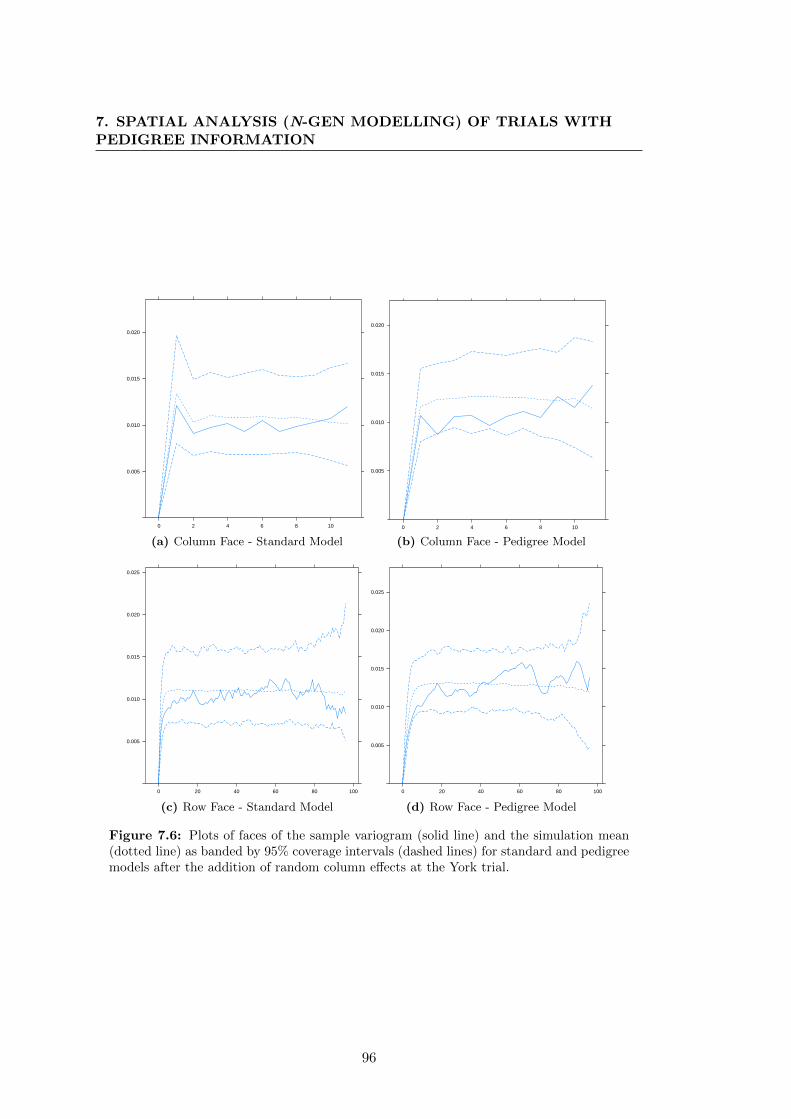
7. SPATIAL ANALYSIS (N-GEN MODELLING) OF TRIALS WITHPEDIGREE INFORMATION
xvar
gam
ma
0.005
0.010
0.015
0.020
0 2 4 6 8 10
(a) Column Face - Standard Model xvar
gam
ma
0.005
0.010
0.015
0.020
0 2 4 6 8 10
(b) Column Face - Pedigree Model
xvar
gam
ma
0.005
0.010
0.015
0.020
0.025
0 20 40 60 80 100
(c) Row Face - Standard Modelxvar
gam
ma
0.005
0.010
0.015
0.020
0.025
0 20 40 60 80 100
(d) Row Face - Pedigree Model
Figure 7.6: Plots of faces of the sample variogram (solid line) and the simulation mean(dotted line) as banded by 95% coverage intervals (dashed lines) for standard and pedigreemodels after the addition of random column effects at the York trial.
96

7.3 Results
7.3.1.1 Model parameters
REML estimates of variance parameters from the sequence of models fitted for the
YORK6 disease nursery are summarized in Table 7.2. REML estimates of error variance
were always lower under the pedigree model than the standard model. REML estimates
of row autocorrelation values were similar across the first two models fitted for standard
(1 and 1a) and pedigree (2 and 2a) models but differed between standard and pedigree
for the last model fitted (1b and 2b) with the correlations being much stronger for the
pedigree model. REML estimates of column autocorrelation values were always larger
and non-negative under the pedigree models than the standard models (Table 7.2). For
standard and pedigree models, the REML estimates of the random column components
were similar at 0.014 and 0.015 respectively.
97

7. SPATIAL ANALYSIS (N-GEN MODELLING) OF TRIALS WITHPEDIGREE INFORMATION
Tab
le7.2
:O
verview
ofth
eseq
uen
ceofm
od
elsfi
ttedfo
rth
eY
ork
trial,
terms
ad
ded
forglob
altren
dan
dex
traneou
svariation
,R
EM
Lestim
ates
of
errorva
rian
ce,auto
correla
tionp
arameters
an
dglo
bal
trend
/ex
tran
eou
svariation
comp
onen
ts.R
EM
Llog-likelih
ood
san
dlo
g-likelih
ood
ratio
testare
also
listedfor
eachm
od
el.
Mod
elG
lobal
trend
Error
Au
tocorrelation
Glob
alR
EM
LL
og-Likelih
ood
&ex
traneou
svariation
variance
Row
Colu
mn
Rd
(Col)
ratiotest
(lr )
Stan
dard
Mod
el10.055
0.910.25
649.51a
lin(R
)+
0.0410.86
-0.04653.0
1blin
(R)
+rd
(C)#
0.0300.27
-0.130.014
666.7p<
0.001P
edig
reeM
od
el20.051
0.900.34
905.62a
lin(R
)0.038
0.870.14
906.52b
lin(R
)+
rd(C
)0.024
0.580.06
0.015923.9
p<
0.001+
lin(R
)in
dica
tesa
fixed
linea
rreg
ression
on
rownum
ber;
#rd
(C)
indica
tesra
ndom
colu
mn
effects.
98

7.3 Results
7.3.2 All trials
Model terms to encompass extraneous variation and non-stationary trend were required
for 4 out of the 10 trials (Table 7.3). YORK6 was the only trial in the data set which
needed more than one term to encompass global and extraneous variation in both row
and column dimensions. Across all trials, the same extraneous variation components
were added to both standard and pedigree models.
In terms of stationary trend, row autocorrelation values were strong (> 0.3) at 4
out of the 10 trials and column autocorrelation values were strong at 2 of the trials
(Table 7.3). Overall, the largest row autocorrelation values was observed at LKBL3
at 0.63 for standard and 0.62 for pedigree models respectively. The largest difference
in row and column autocorrelation values between standard and pedigree models were
observed for the YORK6 and ELMR3 trials (Table 7.3).
An absolute Scres value of 3 was used to determine which data points would be
recognised as outliers. Out of the 10 trials, 6 trials had the same number of outliers
under both standard and pedigree models (BUNT6, LKBL3, MNGN6, PTLI5, SSTL6,
YORK6). However 2 trials, CCRK2 and ELMR3 had more outliers under the standard
model than the pedigree model. A plot of the Scres for the standard and pedigree
models at ELMR3 can be seen in Fig. 7.7. This plot indicates 5 outliers were identified
under the standard model and 3 outliers identified under the pedigree models, of which
2 outliers were in common between both models. Additionally it was observed that the
Scres values corresponding to single replicate entries (black dots) were furthest from
the line of equivalence (y=x), Scres values corresponding to entries with two replicates
were closer to this line, and other colours (i.e yellow dots) were even closer to this line.
This indicates poor agreement between models for single replicate Scres entries.
99

7. SPATIAL ANALYSIS (N-GEN MODELLING) OF TRIALS WITHPEDIGREE INFORMATION
●●
●
●
●
●
●
●
●
●
●
●
●
●●
●
●
●
●
●
●
●
●
●●
●
●
●
●
●
●●
●
●
●
●
●
●
●●
●
●
●
●
●
●
●
●
●
●
●
●●
●
●
●
●●
●
●●
●
●
●
●
●
●
● ●
●
●
●
●
●
●
●
●
●
●
●
●
●
●
●
●●
●
●
●
●
●
●
●●
●
●
●
●
●
●●
●
●
●
●
●●
●
●
●
●
● ●
●
●
●●●
●
●
●
●
●
●
●
●
●
●
●
●
●
●
●
●
●
●
●
●
●
●●
●●
●
●
●
●
●
●
●
●
●
●
●
●
●
●
●
●
●
●
●
●
●
●
●
●
●
●
●
●
●
●
●
●
●
●
●
●
●
●
●
●
●
●
●
●
●
●
●
●
●●
●
●
●
●
●
●●
●
●
●
●
●●
●●
●
● ●
●
●
●
●
●●
●
●
●
●
●●
●
●
●
●
●
●
●
●
●
●
●
●
●
●
●
●
●
●
●
●
●
●
●
●
●
●
●
●
●
●
●●
●
●
●
●
●
●
●
●
●
●
●
●
●
●
●
●
●
●
●
●
●
●
●
●
●
●
●
●
●
●
● ●
●
●●
●
●●
●
●
●
●
●
●
●
●
●
●
●
●
●
●
●
●
●
●
●
●
●●
●
●
●
●
●
●
●●
●
●
●
●
●●
●
●
●
●
●
●
●
●
●
●
●●
●
● ●
●
●
●
●●
●
●
●
●
●
●
●
●
●
●●
●
●
●
●
●
●
●
●
●
●
●
●
●
●●
●
●
●
●
●
●
●
●
●
●
●
●
●
●
●
●
●
●●
●
●
●
●
●
●
●●
●
●
●
●
●
●
●
●
●
●
●
●
●
●
●
●
●
●
●
●
●
● ●
●●
●
●●
●
●
●
●
●●
●
●
●
●
●
●
●
●
●
●
●●
●
●
●
●
●
●
●
●
●
●
●
● ●
●
●
●
●
●
●
●
●
●
●
●
●
●
●
●
●
●
●
●
●
●
●
●
●
●
●
●
●
●
●
●
●
●
●
●
●
●
●
●
●
●
●
●
●
●
●
●
●
●
●
●
●
●
●
●
●
●
●
●
●
●
●
●
●
●
●
●
−4 −2 0 2 4
−4
−2
02
4
Studentised Conditional Residuals − Pedigree Model
Stu
dent
ised
Con
ditio
nal R
esid
uals
− S
tand
ard
Mod
el
Figure 7.7: Outliers detected under standard and pedigree models - Studentisedconditional residuals from AOMM diagnostics for the standard model plotted against Stu-dentised conditional residuals from the pedigree models at the Elmore trial. Scres valuescorresponding to entries with one or two replicates are shown as black and red coloureddots respectively, with other numbers of replicates have differing colours. The solid lineindicates the equivalence, that is y=x. Dashed horizontal and vertical lines indicate theabsolute Scres cut off value of 3.
100

7.4 Discussion
Table 7.3: Spatial modeling of the 2011 growing season trials. REML estimates of errorvariance, autocorrelation parameters for rows/columns, terms added for global trend andextraneous variation and outliers detected for standard (std) and pedigree (ped) models.
Trial Model Error Autocorrelation Global trend & Outliersvariance Row Column extraneous variation detected
ALBR2 std 0.059 0.15 0.10 3ALBR2 ped 0.061 0.24 0.13 4BUNT6 std 0.039 0.19 0.16 rd(R)# 4BUNT6 ped 0.037 0.09 0.14 rd(R) 4CCRK2 std 0.143 -0.01 0.13 11CCRK2 ped 0.126 0.14 0.21 10ELMR3 std 0.080 0.06 0.34 5ELMR3 ped 0.083 0.23 0.39 3LKBL3 std 0.085 0.63 0.14 2LKBL3 ped 0.082 0.62 0.15 2
MNGN6 std 0.091 0.26 0.07 2MNGN6 ped 0.084 0.32 0.09 2
PTLI5 std 0.003 0.35 0.02 4PTLI5 ped 0.003 0.34 0.03 4SSTL6 std 0.040 -0.02 0.25 rd(C)# 1SSTL6 ped 0.041 -0.02 0.33 rd(C) 1
WAGG2 std 0.027 0.05 -0.03 rd(C) 1WAGG2 ped 0.027 0.10 -0.11 rd(C) 2YORK6 std 0.030 0.27 -0.13 lin(R)+ + rd(C) 7YORK6 ped 0.024 0.58 0.06 lin(R) + rd(C) 7
+lin(R) indicates a fixed linear regression on row number; #rd(R) and rd(C) indicates random row
and random column effects respectively.
7.4 Discussion
This chapter illustrates the process of spatial mixed model analysis at a single trial stage
for a series of canola breeding trials from the 2011 growing season. Plant breeding trials
are commonly sown as partially replicated trials, which not only enables the testing of
a maximum number of entries, but also enables the testing of new test crosses with
minimal seed (Cullis et al., 2006). On average 80% of entries within a trial in this data
subset were sown as single replicates (Table 6.2 in Chapter 6). The importance of spatial
models in mixed model analysis is especially illustrated in such plant breeding trials.
With limited replication, these trials attempt to provide enough information for the
selection of entries for commercialization and parents for the next cycle of breeding. As
a result, there is a need to obtain accurate selections, which requires the minimisation
of error, such as environmental heterogeneity. This is evident, as environmental effects
are common in all designed field trials, and if not accounted for can lead to biased
estimates of treatment effects (Basford and Cooper, 1998). The estimation of genetic
merit in annual breeding trials is thus critical for the efficiency of a breeding program
101

7. SPATIAL ANALYSIS (N-GEN MODELLING) OF TRIALS WITHPEDIGREE INFORMATION
and spatial mixed model analysis enables this. However, it has not been addressed in
any published research the impacts of pedigree information on spatial models in p-rep
trials.
The presence of local trend was evident in the 2011 growing season trials, with a
majority of trials indicating large autocorrelation values in the row dimension and a few
trials in the column dimension. In addition, terms for global trend/extraneous variation
components were detected at 4 out of the 10 trials with only the trial at YORK6
needing both linear row and random column components. Hence the majority of trials
presented from a single growing season exhibit different smooth spatial variation and
global trend/extraneous variation. This conforms to previous plant breeding studies
which have also identified the presence of extraneous variation in field experiments in
Australia (Cullis et al., 1998, Gilmour et al., 1997, Smith et al., 2001b,a, Stefanova et al.,
2009) and highlights the importance of detecting spatial variation for plant breeding
trials for improving the accuracy of selections in plant breeding experiments.
The addition of pedigree information to the model resulted in differences at 2 trials
for row autocorrelations and 2 trials for column autocorrelations. This differs from the
study by Oakey et al. (2006), who found that column and row autocorrelations were
similar under the standard and pedigree models. Such a difference can be attributed to
Oakey et al. (2006)’s study being based on wheat breeding trials, which were designed
as nearest neighbour designs with most entries sown in all trials. CBWA’s trial designs
on the other hand were p-rep designs with a majority of entries having 1 or 2 reps
within a trial, and a superblock component. Hence the relationships afforded through
pedigree information would be greater in the CBWA data set than those in Oakey et al.
(2006)’s, resulting in a larger impact on trial variance parameter estimates. Thus the
value of pedigree information is especially demonstrated by the ‘borrowing’ of additional
information from relatives to improve the modeling of entry genetic effects and thus
improving the accuracy of spatial modeling.
Six of the trials had the same number of outliers detected under the pedigree model
and standard models. However the two trials, ELMR3, and CCRK2, had more outliers
detected under the standard model than the pedigree model. For the outliers detected
for each trial (see Table 7.3), some were in common between the models but there were
102

7.4 Discussion
also some that corresponded to different data points unique to the model. From the
plot of Scres residuals under both standard and pedigree models at the ELMR3 trial
(Fig. 7.7), it was also evident that entries with single replicates had poor agreement
between the two models. This would be expected, as the impact of pedigree informa-
tion would be larger for entries with single replicates than for entries that have many
replicates. Hence the impact of pedigree inclusion is especially important for single
replicate entries, which explains entry performance better than the standard model,
which assumes independence of genetic relationships between trial entries. Pedigree
information is thus demonstrated as important in improving the accuracy of outlier
detection.
The spatial mixed model analysis was undertaken at a single trial, for all trials
within the 2011 growing season. It was not extended in this chapter to include dif-
ferences in spatial models that would arise within a MET/FA framework of analysis,
due to issues with the time taken for the analysis. This issue will be examined in more
detail in Chapter 9. An important point is that under a MET analysis, it would be
expected that greater relationships afforded through MET and FA modeling will result
in larger differences between spatial models for standard and pedigree models. This
would be furthered by the fact that p-rep design and superblock components enables
for replication to be balanced across trials, thereby contributing to more information
in the model.
The spatial mixed model analysis from this chapter will be extended in the next
chapter with a MET/FA analysis to obtain breeding program selections. However, it
is important to mention that each trial within a MET requires its own spatial model
since trial errors are characterised by heterogeneous variance or covariances (Crossa
et al., 2006). These result from (i) heterogeneous within site error variances resulting
from site to site variations among plots from properties that impact on the measured
traits, (ii) particular trials and or years showing more genotypic variation and (iii)
heterogeneous covariances among trials arising from similarities between trials based
on environmental factors (Crossa et al., 2006). Hence, the analysis of MET data must
encompass spatial structures to accommodate these sources of extraneous variation,
and the absence of this may result in large experimental error variance components.
103
7. SPATIAL ANALYSIS (N-GEN MODELLING) OF TRIALS WITHPEDIGREE INFORMATION
7.5 Summary
This chapter demonstrated the stages of Ngen analysis and evaluated the impact of
spatial analysis under pedigree models in comparison to standard models at a single
trial, specifically for p-rep designs. From this study, it is evident that pedigree infor-
mation aids in the modeling of spatial errors, by adding information to the analysis
that would otherwise not have been included. Due to common relationships found in
breeding programs, it is evident that pedigree information aids in the explanation of
entry performance. As demonstrated by the differences between spatial models and
outlier detection under standard and pedigree models, it is recommended that base
line Ngen modeling should always include pedigree information for the determination
of trial spatial models.
104

Chapter 8
MET analysis of trials with
pedigree information
8.1 Introduction
The annual aims of CBWA’s canola breeding program are (1) to select entries for pro-
motion or commercialization and (2) to select parents for the next cycle of breeding.
Selections are based on a number of traits, including grain yield, blackleg disease re-
sistance, oil and protein quality, however the primary trait of selection is grain yield.
Such selection is undertaken annually from the analysis of METs located across a broad
range of Australian target environments. The objective is to produce open-pollinated
and F1 hybrid varieties for commercial release, or for use in crossing.
Historically additive and non-additive effects (often referred to as General Com-
bining Ability (GCA) and Specific Combining Ability (SCA) in the literature) are an
important basis for breeders decisions on hybrid breeding strategies (de la Vega and
Chapman, 2006). Additive genetic effects can be viewed as breeding values, as they rep-
resent the heritable component of genetic variation. The derivation of additive genetic
effects is important for breeding objectives and key to maximising breeding progress
(Falconer, 1981).
The performance of entries across locations, that is the magnitude of GxE, is an-
other important source of information. METs are critical in estimation of magnitude
105
8. MET ANALYSIS OF TRIALS WITH PEDIGREE INFORMATION
and patterns of GxE. GxE interactions can be the result of differences in genotypic
adaptation and/or due to heterogeneous environments within targeted areas for se-
lection (Fukai and Cooper, 1995). Cross-over GxE can limit response to selection,
as it complicates the comparisons of entry performance over environments (Argillier
et al., 1994, Cooper and DeLacy, 1994). However an understanding of GxE also allows
breeders to better exploit specific or general adaptation and even identify target envi-
ronment clusters (Bernardo, 2002). Hence an understanding of GxE is an important
component in maintaining genetic gain in selection in plant breeding programs. This
is especially the case where the target environments are diverse, such as in CBWA’s
breeding program, which develops varieties for low to high rainfall cropping zones of
southern Australia.
These selection aims and an understanding of the impact of GxE may be addressed
using the mixed model analysis of MET data developed by Smith et al. (2001b) with
an extension for pedigree information by Oakey et al. (2007). Having demonstrated
the application and process of N-gen modeling in the previous chapter, this chapter
commences with the next step in the mixed model process, that is the genetic mod-
eling (gen-modeling) process for MET data from p-rep trials. This is applied to the
motivating example of CBWA’s 2011 MET and followed by an interpretation of the
impact of environment on selection in CBWA’s breeding program.
8.2 Methods and Materials
8.2.1 Description of data
The motivating data set consists of a subset of the 2011 trial data with corresponding
pedigree file. The pedigree file was obtained using the package ‘Pedicure’ (Butler, 2012)
in R (R Development Core Team, 2012), which limited pedigree data to entries present
in the current data set. A total of 13 generations of pedigree information was available
for this pedigree/data set combination, see Table 6.8, Chapter 6. This consisted of 91
unique mothers and 226 unique fathers with a total of 1544 entries in the pedigree file.
The MET data set consisted of a total 5941 records on 1084 entries.
106

8.2 Methods and Materials
The trial details were as summarized in Chapters 6 and 7. The MET data set had a
total of 10 trials across 10 locations within a single year (growing season). These loca-
tions targeted canola production zones across four Australian states from low to high
rainfall. These ranged from Mingenew W.A (29◦19 S, 115◦16 E) to Croppa Creek NSW
(29◦71 S, 150◦18 E). Annual rainfall and growing season rainfall (May to November)
were obtained for each of the trial locations, from the closest weather station from online
records at the Australian Bureau of Meteorology (http://www.bom.gov.au/climate)
(Table 8.1).
There was good concurrence (commonality) of entries across trials in the MET
data set. A minimum of 141 entries were in common between any pair of trials (upper
triangle Table 8.2). Concurrence of parent entries, that is both males and females, were
high as well with a minimum concurrence of 116 (lower triangle Table 8.2). Overall
there was greater concurrence of parents across trials than entries.
107

8. MET ANALYSIS OF TRIALS WITH PEDIGREE INFORMATION
Tab
le8.1
:L
oca
tionb
asedtria
ld
etails:state,
latitu
de,
lon
gitu
de,
sowin
gan
dh
arvest
dates,
trialm
eanyield
and
rainfa
llfor
CB
WA
’s2011
ME
Ts.
Tria
lT
rial
Sta
teL
atitu
de
Lon
gitu
de
Sow
ing
Harv
estT
rial
mea
nR
ain
fall
(mm
)C
od
ed
ate
date
yield
An
nu
al
Gro
win
gsea
son
AL
BR
2A
lbu
ryN
SW
35◦90
S146◦92
E17/05/11
06/12/11
1.4
7874
420
BU
NT
6B
untin
eW
A29◦95
S116◦29
E11/05/11
01/11/11
1.4
9354
286
CC
RK
2C
rop
pa
Creek
NS
W29◦71
S150◦18
E13/05/11
04/11/11
2.0
3171
433
EL
MR
3E
lmore
VIC
36◦29
S144◦36
E26/05/11
29/11/11
2.1
5539
307
LK
BL
3L
ake
Bola
cV
IC37◦58
S142◦90
E17/05/11
06/12/11
0.9
6554
267
MN
GN
6M
ingen
ewW
A29◦19
S115◦16
E14/05/11
24/10/11
1.9
1469
396
PT
LI5
Pt
Lin
coln
SA
34◦43
S135◦51
E13/05/11
12/11/11
0.6
5565
362
SS
TL
6S
thS
tirling
Ran
ges
WA
34◦57
S118◦27
E11/05/11
30/11/11
0.8
6484
325
WA
GG
2W
agga
WA
34◦93
S147◦35
E12/05/11
23/11/11
0.9
5664
319
YO
RK
6Y
ork
WA
31◦53
S116◦46
E09/05/11
15/11/11
1.3
2460
395
108
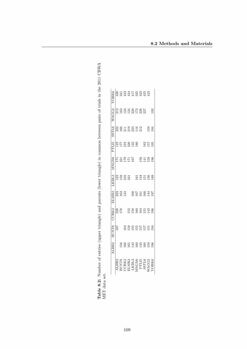
8.2 Methods and Materials
Tab
le8.2
:N
um
ber
ofen
trie
s(u
pp
ertr
iangl
e)an
dp
are
nts
(low
ertr
ian
gle
)in
com
mon
bet
wee
np
air
sof
tria
lsin
the
2011
CB
WA
ME
Td
ata
set.
AL
BR
2B
UN
T6
CC
RK
2E
LM
R3
LK
BL
3M
NG
N6
PT
LI5
SS
TL
6W
AG
G2
YO
RK
6A
LB
R2
167
228
223
123
171
123
222
212
426
BU
NT
6156
178
163
158
231
177
166
163
321
CC
RK
2160
164
124
216
178
218
211
123
423
EL
MR
3165
159
152
221
171
220
219
124
424
LK
BL
3143
155
158
160
167
122
223
220
417
MN
GN
6160
155
160
167
161
180
116
172
335
PT
LI5
143
157
164
161
144
156
212
228
423
SS
TL
6160
157
155
160
151
141
162
227
425
WA
GG
2159
151
143
144
156
158
157
159
423
YO
RK
6196
194
196
197
189
196
195
194
192
109

8. MET ANALYSIS OF TRIALS WITH PEDIGREE INFORMATION
8.2.2 Statistical models
The analysis for a series of t trials, is an extension of the single trial model in Equation
7.3, Chapter 7. This MET model was initially proposed by Smith et al. (2001b), with
an extension for pedigree information developed by Oakey et al. (2007). The MET
model with pedigree information can be written as,
y = Xτ +Zv(ua + ui) +Zpup + e (8.1)
where y = (yT1 ,yT2 , ...,y
Tt )T , that is now a concatenated vector of data of individual
plot yields in t/ha combined across trials. X and Zv, are design matrices for fixed
effects and random genetic effects respectively. τ = (τT1 , τ
T2 , ...., τ
Tt )T is the p × 1
vector of fixed effects, and includes effects such as linear regression on rows associated
with spatial trend; ua = (uaT1 ,ua
T2 , ....,ua
Tt )T is the mt× 1 vector of random additive
genetic effects; ui = (uiT1 ,ui
T2 , ....,ui
Tt )T is the mt× 1 vector of random non-additive
genetic effects; up = (upT1 ,up
T2 , ....,up
Tt )T is the q × 1 vector of random peripheral
effects and e = (eT1 , eT2 , ...., e
Tt )T is the vector of residuals ordered as per the data
vector. Note that the vector of random peripheral effects (up) comprises blocking
effects for each trial and effects such as random row to accommodate spatial trend and
has the associated design matrix Zp. In this data set t = 10 and m = 1544.
The variance model for additive and non-additive genetic effects are:
var (ua) = Gea ⊗A
var (ui) = Gei ⊗ Im
where Ges, s = a, i, is the genetic variance matrix of dimensions t× t, for environments
e, with the main diagonal being the genetic variance for each trial and the off-diagonals
the genetic covariances between pairs of trials. A is as previously defined, the additive
relationship matrix and Im is an identity matrix of order m.
The variance model for errors is the same as in Chapter 7 Equation 7.2, however
the extension across trials using the approach of Smith et al. (2001b) is,
var (e) = R = ⊕tj=1Rj
110

8.2 Methods and Materials
where Rj is the variance matrix for the errors for the jth trial (j = 1, .., t). This
extension, enables a separate spatial covariance structure for error in each trial.
The variance model for the random peripheral effects are:
var (up) = Gp = ⊕tj=1 ⊕
bjl=1 σ
2pjlIqjl
where each trial has a maximum of bj random peripheral terms and the lth term (l =
1, ..., bj) has qjl effects and an associated variance component of σ2pjl
.
The first step of the analysis is to check for outliers and the adequacy of the spatial
model for each trial. As this was already undertaken in Chapter 7, the process was
only re-examined for the MET data set. This was achieved using a diagonal model for
the genetic variance matrix (Ges, s = a, i), so that,
Gea = diag {σ2aj}
Gei = diag {σ2ij}
where σ2aj is the additive genetic variance and σ2
ij is the non-additive genetic variance
of each trial, j for j = 1, ..., t. The diagonal model is the equivalent of running t = 10
individual trial analyses as undertaken in the previous chapter. The spatial models
were adequate and the same terms for global trend and extraneous variation for each
trial in Chapter 7 Table 7.3, were included in this MET analysis.
As in Chapter 7, AOMM statistics (Smith et al. unpublished paper) were used
to identify outliers in the 2011 trial data. An absolute Scres value of 3 was used
to diagnose outliers. Identified outliers were then examined in the datafile, with the
criterion for omission based on the Scres of other replicates within the trial and if
these were not present, the Scres of sister-lines with common parentage. For example
consider the trial MNGN6, the entry CBD1310 at column 9 row 24, was dropped after
identifying the Scres of its sister lines (i.e; they have the same mother). The Scres for
the sisterlines, were 3.63 and 0.86 respectively (see Table 8.3) compared to -5.67 for
the identified outlier. In concurrence with this outlier diagnostic, the detected outliers
were also confirmed with the plant breeder as erroneous, and then set to a missing
value delimiter in the data file.
111
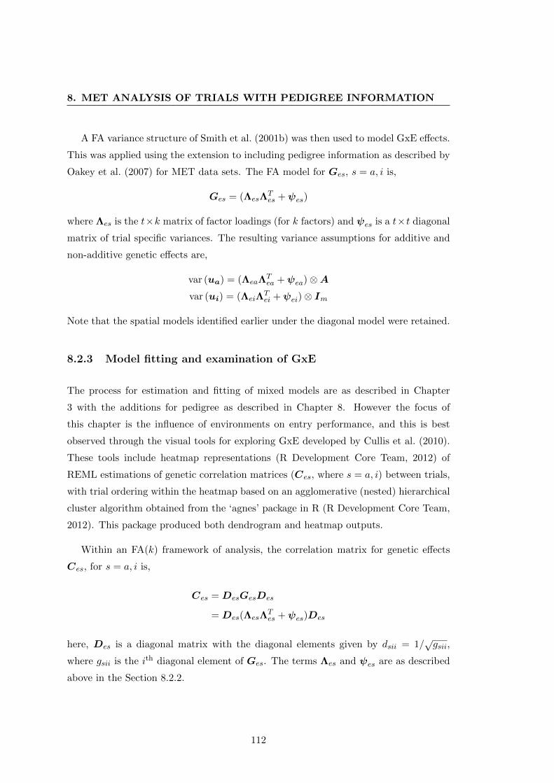
8. MET ANALYSIS OF TRIALS WITH PEDIGREE INFORMATION
A FA variance structure of Smith et al. (2001b) was then used to model GxE effects.
This was applied using the extension to including pedigree information as described by
Oakey et al. (2007) for MET data sets. The FA model for Ges, s = a, i is,
Ges = (ΛesΛTes +ψes)
where Λes is the t×k matrix of factor loadings (for k factors) and ψes is a t×t diagonal
matrix of trial specific variances. The resulting variance assumptions for additive and
non-additive genetic effects are,
var (ua) = (ΛeaΛTea +ψea)⊗A
var (ui) = (ΛeiΛTei +ψei)⊗ Im
Note that the spatial models identified earlier under the diagonal model were retained.
8.2.3 Model fitting and examination of GxE
The process for estimation and fitting of mixed models are as described in Chapter
3 with the additions for pedigree as described in Chapter 8. However the focus of
this chapter is the influence of environments on entry performance, and this is best
observed through the visual tools for exploring GxE developed by Cullis et al. (2010).
These tools include heatmap representations (R Development Core Team, 2012) of
REML estimations of genetic correlation matrices (Ces, where s = a, i) between trials,
with trial ordering within the heatmap based on an agglomerative (nested) hierarchical
cluster algorithm obtained from the ‘agnes’ package in R (R Development Core Team,
2012). This package produced both dendrogram and heatmap outputs.
Within an FA(k) framework of analysis, the correlation matrix for genetic effects
Ces, for s = a, i is,
Ces = DesGesDes
= Des(ΛesΛTes +ψes)Des
here, Des is a diagonal matrix with the diagonal elements given by dsii = 1/√gsii,
where gsii is the ith diagonal element of Ges. The terms Λes and ψes are as described
above in the Section 8.2.2.
112
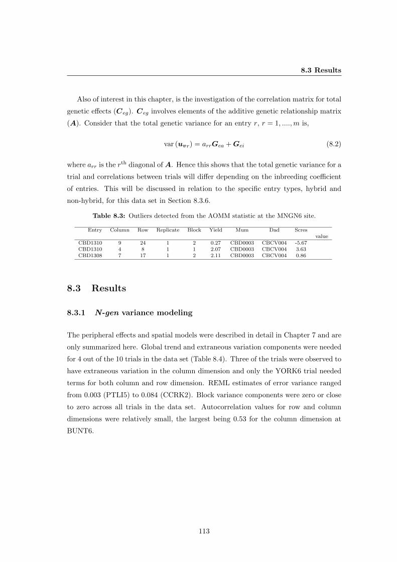
8.3 Results
Also of interest in this chapter, is the investigation of the correlation matrix for total
genetic effects (Ceg). Ceg involves elements of the additive genetic relationship matrix
(A). Consider that the total genetic variance for an entry r, r = 1, ....,m is,
var (uvr) = arrGea +Gei (8.2)
where arr is the rth diagonal ofA. Hence this shows that the total genetic variance for a
trial and correlations between trials will differ depending on the inbreeding coefficient
of entries. This will be discussed in relation to the specific entry types, hybrid and
non-hybrid, for this data set in Section 8.3.6.
Table 8.3: Outliers detected from the AOMM statistic at the MNGN6 site.
Entry Column Row Replicate Block Yield Mum Dad Scresvalue
CBD1310 9 24 1 2 0.27 CBD0003 CBCV004 -5.67CBD1310 4 8 1 1 2.07 CBD0003 CBCV004 3.63CBD1308 7 17 1 2 2.11 CBD0003 CBCV004 0.86
8.3 Results
8.3.1 N-gen variance modeling
The peripheral effects and spatial models were described in detail in Chapter 7 and are
only summarized here. Global trend and extraneous variation components were needed
for 4 out of the 10 trials in the data set (Table 8.4). Three of the trials were observed to
have extraneous variation in the column dimension and only the YORK6 trial needed
terms for both column and row dimension. REML estimates of error variance ranged
from 0.003 (PTLI5) to 0.084 (CCRK2). Block variance components were zero or close
to zero across all trials in the data set. Autocorrelation values for row and column
dimensions were relatively small, the largest being 0.53 for the column dimension at
BUNT6.
113

8. MET ANALYSIS OF TRIALS WITH PEDIGREE INFORMATION
Tab
le8.4
:S
patia
lm
od
eling
forth
e20
11M
ET
.R
EM
Lestim
ates
of
error,
blo
ckan
dau
tocorrelation
param
etersfor
rows
and
colu
mn
s.T
erms
ad
ded
forglob
altren
dor
extran
eous
varia
tion
an
dth
enu
mb
erof
outliers
removed
.
Erro
rB
lock
Au
tocorrelation
Glob
altren
d&
Nu
mb
erof
Colu
mn
Row
extran
eous
variationterm
sou
tliers
AL
BR
20.0
60.00
0.130.26
1B
UN
T6
0.0
30.00
0.100.22
rd(R
)#
2C
CR
K2
0.080.00
0.200.16
EL
MR
30.08
0.000.34
0.262
LK
BL
30.0
80.00
0.110.59
MN
GN
60.0
70.01
0.080.32
1P
TL
I50.0
00.00
0.040.33
1S
ST
L6
0.030.00
0.410.08
rd(C
)#
1W
AG
G2
0.020.00
-0.040.24
rd(C
)2
YO
RK
60.0
20.00
0.000.67
lin(R
)+
&rd
(C)
1+
lin(R
)in
dica
tesa
fixed
linea
rreg
ression
on
rownum
ber;
#rd
(R)
and
rd(C
)in
dica
tesra
ndom
rowand
random
colu
mn
effects
respectiv
ely.
114

8.3 Results
8.3.2 Outliers
All trials except CCRK2 and LKBL3 had at least one outlier removed (Table 8.4).
A majority of plots in column 1 of the CCRK2 trial were identified as outliers. This
was confirmed with the plant breeder as resulting from an issue of uneven germination
in this column (C Beeck, pers.comm.). As a result, this first column of the trial was
dropped; that is set to a missing value delimiter for this trial.
8.3.3 FA Model
Commencing with the base line diagonal model for Ges, an FA(1) followed by an FA(2)
structure were then fitted. There was an increase in log-likelihood (lr) from the diagonal
model up to the FA(2) (Table 8.6). The FA(2) model provided a superior fit (P<0.001)
and accounted for 79.88% of trial additive genetic variance and 76.25% of trial non-
additive genetic variance (Table 8.6). Due to computational limitations impacting on
time to analysis, the FA(2) was the last model fitted. Note however, that on average
a large percentage of both additive and non-additive genetic variance is explained by
the FA(2).
REML estimates of the percent variance accounted by the two factors in the FA(2)
model for additive genetic effects at each trial are summarized in Table 8.5. A large
proportion of the additive trial variance was accounted for by the first factor at the
trials ALBR2, BUNT6, CCRK2, ELMR3 and YORK6, which all had greater than 70%
explained. The percent variance accounted for by the first factor was poor for the trials
PTLI5 and SSTL6 (Table 8.5). The remaining trials, LKBL3, MNGN6 and WAGG2
had greater than 50% variance accounted for by the first factor. The second factor
however accounted for a large amount of variance for the trials BUNT6 and SSTL6,
22.06 and 34.87 respectively. Total percent variance under the FA(2) model for additive
effects was 100% for ALBR2, BUNT6 and CCRK2. At all other trials, the total percent
variance explained by the FA(2) for additive trial effects was greater than 70% except
for MNGN6 (68.18%) and PTLI5 (12.62%).
REML estimates of percent variance accounted by the two factors in the FA(2) model
for non-additive genetic effects at each trial are summarized in Table 8.5. The percent
115
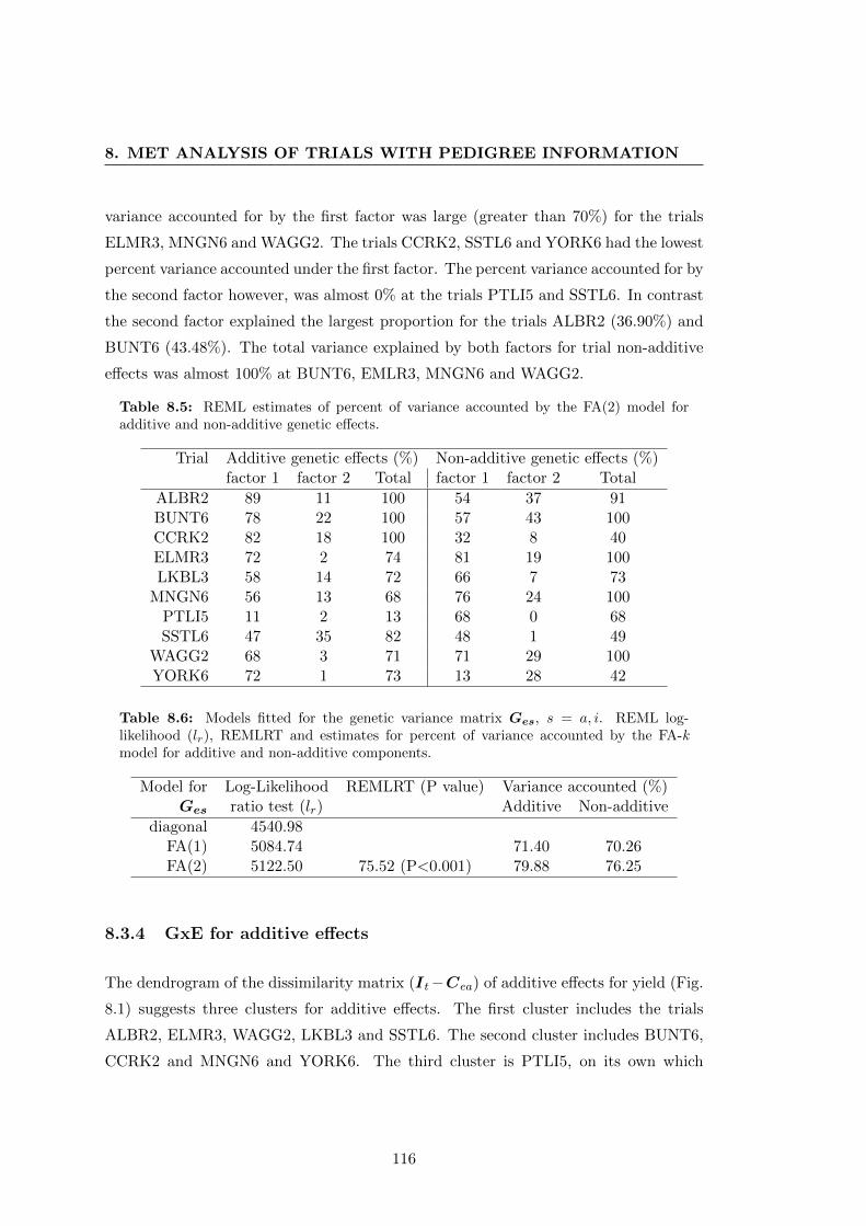
8. MET ANALYSIS OF TRIALS WITH PEDIGREE INFORMATION
variance accounted for by the first factor was large (greater than 70%) for the trials
ELMR3, MNGN6 and WAGG2. The trials CCRK2, SSTL6 and YORK6 had the lowest
percent variance accounted under the first factor. The percent variance accounted for by
the second factor however, was almost 0% at the trials PTLI5 and SSTL6. In contrast
the second factor explained the largest proportion for the trials ALBR2 (36.90%) and
BUNT6 (43.48%). The total variance explained by both factors for trial non-additive
effects was almost 100% at BUNT6, EMLR3, MNGN6 and WAGG2.
Table 8.5: REML estimates of percent of variance accounted by the FA(2) model foradditive and non-additive genetic effects.
Trial Additive genetic effects (%) Non-additive genetic effects (%)factor 1 factor 2 Total factor 1 factor 2 Total
ALBR2 89 11 100 54 37 91BUNT6 78 22 100 57 43 100CCRK2 82 18 100 32 8 40ELMR3 72 2 74 81 19 100LKBL3 58 14 72 66 7 73
MNGN6 56 13 68 76 24 100PTLI5 11 2 13 68 0 68SSTL6 47 35 82 48 1 49
WAGG2 68 3 71 71 29 100YORK6 72 1 73 13 28 42
Table 8.6: Models fitted for the genetic variance matrix Ges, s = a, i. REML log-likelihood (lr), REMLRT and estimates for percent of variance accounted by the FA-kmodel for additive and non-additive components.
Model for Log-Likelihood REMLRT (P value) Variance accounted (%)Ges ratio test (lr) Additive Non-additive
diagonal 4540.98FA(1) 5084.74 71.40 70.26FA(2) 5122.50 75.52 (P<0.001) 79.88 76.25
8.3.4 GxE for additive effects
The dendrogram of the dissimilarity matrix (It−Cea) of additive effects for yield (Fig.
8.1) suggests three clusters for additive effects. The first cluster includes the trials
ALBR2, ELMR3, WAGG2, LKBL3 and SSTL6. The second cluster includes BUNT6,
CCRK2 and MNGN6 and YORK6. The third cluster is PTLI5, on its own which
116
8.3 Results
appears to be unrelated to these two major clusters, indicating poor agreement for
additive effects.
The heatmap for additive correlations (Fig. 8.2) confirms high correlations within
clusters and moderate to weak correlations between clusters. PTLI5 had correlations
of less than 0.35 with all other trials. SSTL6 showed poor agreement (less than 0.40
correlation) with 4 trials and greater than 0.50 correlations with the remainder trials.
The presence of the two main clusters with low to moderate correlations between them
indicates the presence of GxE within this single year MET.
ALB
R2
ELM
R3
WA
GG
2
LKB
L3
SS
TL6
BU
NT
6
CC
RK
2
MN
GN
6
YO
RK
6
PT
LI5
0.0
0.2
0.4
0.6
Dendrogram of agnes(x = dis.mat, diss = T)
Agglomerative Coefficient = 0.7dis.mat
Hei
ght
Figure 8.1: Dendrogram of the dissimilarity matrix (It−Cea) of additive effectsfor yield. -
117

8. MET ANALYSIS OF TRIALS WITH PEDIGREE INFORMATION
MNG
N6
PTLI5
YORK6
MNGN6
CCRK2
BUNT6
SSTL6
LKBL3
WAGG2
ELMR3
ALBR2
ALBR
2
ELM
R3
WAG
G2
L
KBL3
SS
TL6
BU
NT6
CC
RK2
YOR
K6
PTL
I5
−1.0
−0.5
0.0
0.5
1.0
C1
C2
C3
Figure 8.2: Heatmap of the REML estimate of the additive genetic correlationmatrix (Cea) - The trials are as ordered as in the dendrogram in Fig. 8.1 and the keyindicates the correlation scale.
118
8.3 Results
8.3.5 GxE for non-additive effects
Dendrogram of the dissimilarity matrix (It −Cei) of trial non-additive genetic effects
for yield can be seen in Fig. 8.3. The dendrogram suggests the presence of 2 clusters.
The first consists of the trials ALBR2, BUNT6, MNGN6, CCRK2, YORK6 and the
second cluster consists of the trials ELMR3, WAGG2, LKBL3, PTLI5 and SSTL6.
There appears to be good agreement of trials within a cluster.
The heatmap for non-additive correlations (Fig. 8.4) reflects the 2 clusters seen
in the dendrogram. A majority of the trials are highly correlated (greater than 0.70)
for non-additive effects. The exception to this is CCRK2 and YORK6 which had
correlations less than 0.54 for 3 trials and 2 trials respectively. Similar to additive
effects, the heatmap for non-additive effects indicates the presence of GxE by the
presence of two clusters which are not directly correlated with each other.
Both the additive and non-additive genetic correlations between trials are summa-
rized in Table 8.7. At a majority of trials the non-additive genetic correlations were
smaller than the corresponding trial additive genetic correlations. The only exceptions
to these were the trials MNGN6 and PTLI5, which appeared to have higher non-additive
genetic correlations than additive genetic correlations across trials.
119

8. MET ANALYSIS OF TRIALS WITH PEDIGREE INFORMATION
ALB
R2
BU
NT
6
MN
GN
6
CC
RK
2
YO
RK
6
ELM
R3
WA
GG
2
LKB
L3
PT
LI5
SS
TL6
0.0
0.1
0.2
0.3
0.4
0.5
0.6
Dendrogram of agnes(x = dis.mat, diss = T)
Agglomerative Coefficient = 0.68dis.mat
Hei
ght
Figure 8.3: Dendrogram of the dissimilarity matrix (It − Cei) of trial non-additive genetic effects for yield -
120
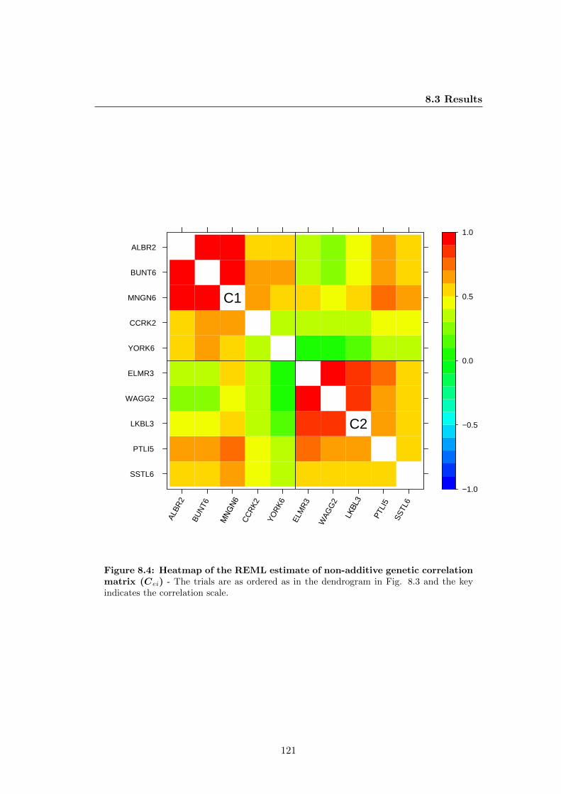
8.3 Results
ALB
R2
B
UN
T6
SSTL6
PTLI5
LKBL3
WAGG2
ELMR3
YORK6
CCRK2
MNGN6
BUNT6
ALBR2
C
CR
K2
YO
RK6
E
LMR
3
WAG
G2
L
KBL3
PTLI
5
SST
L6
−1.0
−0.5
0.0
0.5
1.0
C1
C2
MNG
N6
Figure 8.4: Heatmap of the REML estimate of non-additive genetic correlationmatrix (Cei) - The trials are as ordered as in the dendrogram in Fig. 8.3 and the keyindicates the correlation scale.
121

8. MET ANALYSIS OF TRIALS WITH PEDIGREE INFORMATION
Tab
le8.7
:R
EM
Lestim
ates
ofth
egen
eticcorrelatio
nm
atrix
for
ad
ditive
effects
(up
per
triangle)
and
non
-add
itiveeff
ectsb
etween
trials(low
ertrian
gle).
AL
BR
2B
UN
T6
CC
RK
2E
LM
R3
LK
BL
3M
NG
N6
PT
LI5
SS
TL
6W
AG
G2
YO
RK
6
AL
BR
20.68
0.720.85
0.840.59
0.350.84
0.840.77
BU
NT
60.9
50.99
0.680.50
0.820.22
0.330.64
0.80C
CR
K2
0.5
90.61
0.710.54
0.830.23
0.370.67
0.81E
LM
R3
0.3
90.38
0.380.70
0.580.30
0.670.72
0.71L
KB
L3
0.4
40.4
40.39
0.840.44
0.300.74
0.700.61
MN
GN
60.9
40.98
0.630.57
0.580.19
0.300.55
0.67P
TL
I50.6
10.6
20.47
0.740.67
0.720.31
0.290.26
SS
TL
60.57
0.580.42
0.580.54
0.650.57
0.670.52
WA
GG
20.2
90.28
0.320.99
0.820.47
0.700.53
0.68Y
OR
K6
0.590.6
30.36
0.090.16
0.580.31
0.300.02
122

8.3 Results
8.3.6 GxE for total genetic effects
Recall that the correlation matrix for total genetic effects, Ceg, is dependent on values
of the additive relationship matrix, arr, see Equation 8.2. In this section three different
cases of arr values are considered: based on all entries (which is the standard case),
hybrid entries only and non-hybrid entries only. This approach is warranted based on
the unique make up of the motivational data set, as 555 (51%) of entries were hybrids
(0 inbreeding) and the remainder entries had varying levels of inbreeding, reflected by
their Fgen value and corresponding Fj (Table 8.8).
Table 8.8: Levels of inbreeding (Fgen) for entries in the 2011 MET. Specific Fgen valueswere previously explained in Table 6.7, Chapter 6.
Fgen Number of entries
0.00 1970.74 10.90 110.94 12.00 13.00 354.00 2827.00 110.00 555
8.3.6.1 Total genetic effects: all entries
In this case, Ceg is based on the average inbreeding coefficient of all entries in the
pedigree. Hence arr was evaluated at a = 1.82. This was the method used by Cullis
et al. (2010), Oakey et al. (2007) and Crossa et al. (2006).
The heatmap of total genetic correlations across all entries, suggests the presence of
3 clusters (Fig. 8.5). The first cluster consists of the trials ALBR2, SSTL6, ELMR3,
WAGG2 and LKBL3. The second cluster consists of the trials BUNT6, CCRK6,
MNGN6 and YORK6, which are all located in W.A except for CCRK2. PTLI5 appears
to have its own cluster, indicating poor agreement for total genetic correlations with
the other trial trials. There is close agreement of trials within clusters and moderate
agreement between clusters. The exception is the trial PTLI5, which appears to be
123

8. MET ANALYSIS OF TRIALS WITH PEDIGREE INFORMATION
weakly correlated with a majority of other trials (correlations are less than 0.35 across
all trials).
BU
NT6
C
CR
K2
P
TLI5
E
LMR
3
S
STL6
ALB
R2
PTLI5
YORK6
MNGN6
CCRK2
BUNT6
LKBL3
WAGG2
ELMR3
SSTL6
ALBR2
LK
BL3
M
NG
N6
Y
ORK6
−1.0
−0.5
0.0
0.5
1.0
C1
C2
C3
WAG
G2
Figure 8.5: Heatmap of the REML estimate of the total genetic correlationmatrix (Ceg, where a = 1.82) - The key indicates the correlation scale.
8.3.6.2 Total genetic effects: hybrid entries & non-hybrid entries
In this section, Ceg is based on the average inbreeding of hybrid entries only and then
non-hybrid entries only in the pedigree. For hybrid entries, arr is evaluated at ah = 1.12
and for non-hybrid entries arr is evaluated at anh = 1.97.
Total genetic correlations across trials for hybrid and non-hybrid entries were sum-
marised in Table 8.9. There were no large differences for total genetic correlations across
124

8.3 Results
trials for hybrid entries (lower triangle) and non-hybrid entries (upper triangle). The
clustering for hybrids and non-hybrids were the same as that obtained for total genetic
effects across all entries. That is 3 clusters were suggested, the first cluster consists of
the trials ALBR2, SSTL6, ELMR3, WAGG2 and LKBL3. The second cluster consists
of the trials BUNT6, CCRK6, MNGN6 and YORK6. The third cluster consists only
of PTLI5.
125

8. MET ANALYSIS OF TRIALS WITH PEDIGREE INFORMATION
Tab
le8.9
:R
EM
Lestim
atesof
the
total
genetic
correla
tion
matrix
for
the
2011
ME
T.
Th
elow
ertrian
glecon
sistsof
totalgen
eticco
rrelation
sb
etween
trialsfo
rhyb
riden
triesan
dth
eu
pp
ertria
ngle
con
sistsof
tota
lgen
eticcorrelation
sb
etween
trialsfor
non
-hyb
riden
tries.
AL
BR
2B
UN
T6
CC
RK
2E
LM
R3
LK
BL
3M
NG
N6
PT
LI5
SS
TL
6W
AG
G2
YO
RK
6
AL
BR
20.7
40.72
0.740.69
0.690.44
0.590.71
0.65B
UN
T6
0.6
70.89
0.710.53
0.810.29
0.470.67
0.79C
CR
K2
0.630.84
0.690.51
0.790.28
0.460.65
0.77E
LM
R3
0.730.68
0.640.66
0.660.42
0.570.68
0.63L
KB
L3
0.7
00.49
0.450.70
0.510.49
0.600.64
0.47M
NG
N6
0.6
50.80
0.760.65
0.500.29
0.450.62
0.70P
TL
I50.48
0.2
90.26
0.480.55
0.310.41
0.410.26
SS
TL
60.61
0.450.42
0.610.64
0.450.46
0.550.42
WA
GG
20.7
00.6
40.60
0.700.68
0.620.47
0.590.59
YO
RK
60.59
0.750.72
0.590.44
0.680.26
0.400.56
126

8.3 Results
8.3.7 Selection
The dual aims of a plant breeding program are parental selection and entry promotion.
In this section, it is outlined how the predictions from the MET/FA analysis with
pedigree information can be used for the basis of such selection decisions. The relevant
predictions are the so-called regression BLUPs (referred to as Reg-BLUPs) (Cullis
et al., 2010). Reg-BLUPs were obtained for each entry across each trial in the MET
and averaged across all trials belonging to the cluster groups suggested for additive
(see, Section 8.3.4) and total genetic effects (see, Section 8.3.6). As Reg-BLUPS were
averaged for a cluster, they will be referred to as C-BLUPs. The actual interpretation
of what these cluster groups represent will be considered in detail in the discussion
section.
8.3.7.1 Commercial selection
Commercial selection is based on the total genetic effect for two potential market seg-
ments: hybrid entries and non-hybrid entries. Given a selection target of the top 10
entries (this is an arbitrary number and can vary with breeding program strategy) this
following section considers comparisons between entries within an entry segment
Considering only the hybrid entries, C-BLUPs for total genetic effect were plotted
for the two main clusters, that is excluding the singleton cluster at PTLI5, see Fig.
8.6. The vertical and horizontal lines indicate the top 10 entries that would be selected
for each cluster. Entries on the right hand side of the vertical line indicate the top
10 entries with high total genetic C-BLUPs in Cluster 1 and the entries above the
horizontal line indicate the top 10 entries with high total genetic C-BLUPs for Cluster
2. Of these top 10 entries for each cluster group 6 entries in the top right hand corner
had the highest total genetic C-BLUPs for both cluster groups. This indicates that
there are 4 entries that would be selected for one cluster and not the other. There
was also a large amount of GxE present, indicated by the lack agreement of C-BLUPs
between cluster groups.
127
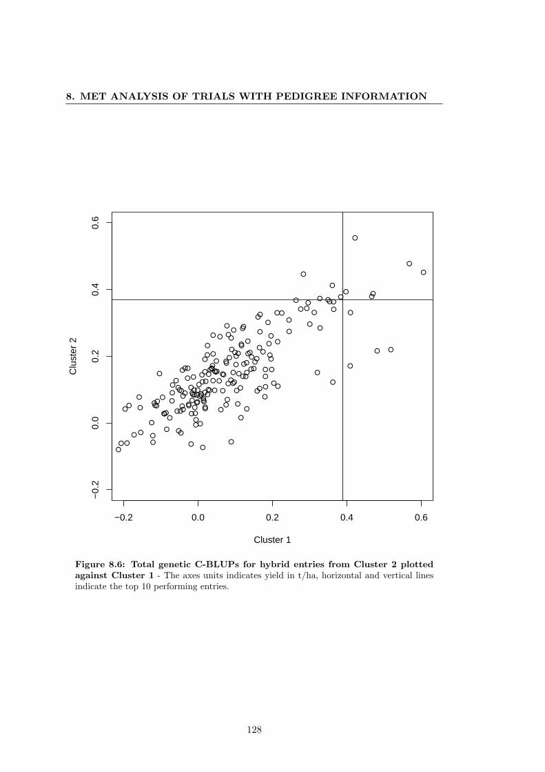
8. MET ANALYSIS OF TRIALS WITH PEDIGREE INFORMATION
●
●
●
●
●
●●
●
●
●
●
●
●
●
●●
●
●
●●
●
●
●
●
●
●●
●
●
●
●
●
●
●
●
●
●
●
●
●
● ●
●
●
●
●
●
●
●
●
●
●
●
●
●
●
●
●
●
●
●
●
●
●
●
● ●
● ●
●
●
●
●
●
●
●
●
●●
●●
●
●
●
●
●
●
●
●●
●●
●
●
●
●
●
●
●
●
●●
●●
●●
●
●
●
●
●
●
● ●
●
●
●●
●
●
●
●
●
●
●
●
● ●
●
●
●
● ●
●
●
●
●
●
●
●
●
●
●
●
●
●
●
●
●
●
●
●
●
●●
●
●
●
●
●
●
●
●
●
●
●
● ●
●
●
●
●
●
●
●●
● ●
●
●
●
●
●
●
●
● ●
●
● ●
●
●●
●
●
●●
−0.2 0.0 0.2 0.4 0.6
−0.
20.
00.
20.
40.
6
Cluster 1
Clu
ster
2
Figure 8.6: Total genetic C-BLUPs for hybrid entries from Cluster 2 plottedagainst Cluster 1 - The axes units indicates yield in t/ha, horizontal and vertical linesindicate the top 10 performing entries.
128

8.3 Results
For the non-hybrid entries, C-BLUPs for total genetic effect were plotted for the
two main clusters, again excluding the singleton cluster at PTLI5, see Fig. 8.7. Only
2 entries were located in the top right hand corner indicating the highest C-BLUPs
across both cluster groups. Entries on the right hand side of the vertical line and above
the horizontal line indicate the top 10 entries with the highest C-BLUPs for Cluster
1 and Cluster 2 respectively. Considering the top 10 entries selected from this plot, 8
entries would be selected for one cluster and not the other.
●
●
●
●
●
●
●
●
●
●
●
●
●
●
●
●
●
●
●
●
●
●
● ●
●
●
●
●
●
●
●
●
●
●
●
● ●
●
●
●
●●
●
●
●●
●
●
●
●
●
●
●●
●
●
●
●
●●●
●
●
●
●
●●
●
●
●
● ●
●
●
●
●
●
●
●
●●
●
●
●
●
●
●
●
●
●
●
●
●
●
●●
●
●●
●
●
●
●
●
●
●
●
●
●
●
●
●
●
●
●
●
●
●
●
●
●
●
●
● ●
●
●●
●
●
●
●
●●
●
●
●
●
●
●
●
●
●
●
●●
●
●
●
●
●
●
●
●
●
●
●
●
●
● ●
●
●●
●
●
●
●
●
●
●
●
●
●
●
●
●
●
●
●
●
●●
●
●
●
●
●
●
●
●
●
●
●
●
●
●
●
●
●
●
●
●
●
●
●
●
●
●●
●
●
●
●
●
●
●
●● ●
●
●
●
●
●
●
●●
●
●
●●
●
●
●
●
●
●●
●
●
●
●
●
●
●
●
●
●
●
●
●
●
●
●
●
●
●
●●●
●
●
●
●
●
●
●
●
●
●
●
●
●
●
●
●
●
●
●
●
●
●
●
●
●
●
●
●
●
●
●
●
●
● ●
●
●
●
●
●
●
●
●
●
●
●
●
●●
●
●
●●
●
●
●
●
●
●
●
●
●●
●
●
●
●
●
●
●
●
●
●
●
●
●●
●
●
●
●
●
●
●
●
●
●
●
●
●
●
●
●
●
●
●
●
●
●
●
●
●
●
●
●
●
●
●
●
●
●
●
●
●
●
●
●
●
●
●
●
●
●
●
●
●
●
●
●
●●
●
●
●
●
●
●●
● ●
●
●
●
●
●
●
●
●
●
●
●
●
●
●
●
●
●
●
●
●
●
●
●
●
●
●
●
●
●
●
●
●
●
●
●
●
●
●●
●
●
●
●
●
●
●
●●
●
● ●
●
●
●
●
●
●
●
●
●
●
●
●
●
●●
●
●
●
●
●
●
●
●
●
● ●
●
●
●
●
●
●
●
●
●●
●
●
●
●
●
●●
●
●
●
●●
●
●
●
●
●
● ●
●●
●
●●
●
●●
●
●
●
●
●
●
●
●
●
●
●
●
●
●
●
●
●●
●
●
●
●
●
●
●
●
●
●
● ●
●
●
●
●
●
●
●
●●
●
●
●
●
●
●●
●
●
●
●●●
●
●
●
●
●
●
●●
●
●
●
●
●
●
●
●
●
●
●
●
●
●
● ●●
●
●
●
●
● ●
●
●
●
●
●
● ●
●
●
●●
●
●
●
●
●
●
●
●
●
●
●
●●
●
●
●
●
●
●
●
●
●
●
●
●
●
●●
●
●
●
●
●
●
●
●
●
●
●
●
●
●
●
●
●
●●
●
●
●
●
●
●●
●
●
●●●
●
●
●
●
●
●
●
●
●●
●
●
●
●
●
●
●
●
●●
●
●
●● ●
●
●
●
●
●
●
●
●
●
●●
●
●
●
●
●
●
●
●
●
●●
●
●
●
●
●
●
● ●
●
●
●
●
●
●●
●●
●
●
●
●●
●
●●
●
●
●
●●
●
●●
●● ●
●
● ●
●●
●
●
●
●●
●
●
●
●
●
●
●
●●
●
●
●
●
●
●
●
●●
●
●
●●
●
●●
●
●
●
●
●
●
●
●
●
●
●
●
●
●
●
●
●
●
●
●
●●
●
●
●
●
●
●
●
●
●
●
●
●
●
●
●
●
●
●
●
●
●
●
●●
●●
●
●
●
●
●
●
●
●
●
●
●
●
●
●
●
●
●
●
●●
●
●
●
●
●
●
●
●
●
●
●
●
●
●
●
●
●
●
●
●
●
●●
●
●
●●
●
●
●
●
●●
−0.8 −0.6 −0.4 −0.2 0.0 0.2 0.4
−0.
8−
0.6
−0.
4−
0.2
0.0
0.2
0.4
Cluster 1
Clu
ster
2
Figure 8.7: Total genetic C-BLUPs for non-hybrid entries from Cluster 2 plot-ted against Cluster 1 - The axes units indicates yield in t/ha, horizontal and verticallines indicate the top 10 performing entries.
129
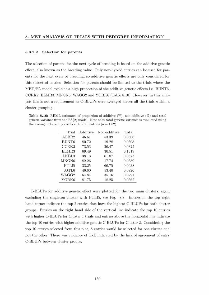
8. MET ANALYSIS OF TRIALS WITH PEDIGREE INFORMATION
8.3.7.2 Selection for parents
The selection of parents for the next cycle of breeding is based on the additive genetic
effect, also known as the breeding value. Only non-hybrid entries can be used for par-
ents for the next cycle of breeding, so additive genetic effects are only considered for
this subset of entries. Selection for parents should be limited to the trials where the
MET/FA model explains a high proportion of the additive genetic effects i.e. BUNT6,
CCRK2, ELMR3, MNGN6, WAGG2 and YORK6 (Table 8.10). However, in this anal-
ysis this is not a requirement as C-BLUPs were averaged across all the trials within a
cluster grouping.
Table 8.10: REML estimates of proportion of additive (%), non-additive (%) and totalgenetic variance from the FA(2) model. Note that total genetic variance is evaluated usingthe average inbreeding coefficient of all entries (a = 1.82).
Trial Additive Non-additive Total
ALBR2 46.61 53.39 0.0506BUNT6 80.72 19.28 0.0508CCRK2 73.53 26.47 0.0325ELMR3 69.49 30.51 0.1319LKBL3 38.13 61.87 0.0573
MNGN6 82.26 17.74 0.0589PTLI5 33.25 66.75 0.0038SSTL6 46.60 53.40 0.0826
WAGG2 64.84 35.16 0.0291YORK6 81.75 18.25 0.0562
C-BLUPs for additive genetic effect were plotted for the two main clusters, again
excluding the singleton cluster with PTLI5, see Fig. 8.8. Entries in the top right
hand corner indicate the top 2 entries that have the highest C-BLUPs for both cluster
groups. Entries on the right hand side of the vertical line indicate the top 10 entries
with higher C-BLUPs for Cluster 1 trials and entries above the horizontal line indicate
the top 10 entries with higher additive genetic C-BLUPs for Cluster 2. Considering the
top 10 entries selected from this plot, 8 entries would be selected for one cluster and
not the other. There was evidence of GxE indicated by the lack of agreement of entry
C-BLUPs between cluster groups.
130

8.3 Results
●
●
●
●
●
●
●
●●
●
●
●
●
●
●
●
●●
●
●
●
●
●
●
●
●
●
●
●
●
●
●
●
●
●
● ●
●
●
●
●●
●
●
●
●
●
●
●
●
●
●
●●
●
●
●
●
●
●●
●
●
●
●
●●
●
●
●
●
●
●
●
●
●
●
●
●●
●
●
●●
●
●
●
●
●
●
●
●
●
●●
●
●
●●
●
●
●
●
●
● ●
●
●●
●
●
●
●●
●
●
●
●
●●
●
●
●
●●
●
●
●
●
●
●
●
● ●
●
●
●
●
●
●
●
●
●
●
●
●
●
●
●
●
●●
●
●●
●
●
●
●
●●
●
● ●
●
●
●
●
●●
●
●
●
●●
●
●
●
●
●
●
●●
●
●
●
●
●
●
●
●●
●
●
●
●
●
●
●
●
●
●
●
●
●
●
●
●
●
●
●
●
●
●
●
●
●
●●●
●
●
●
●
●
●
●
●
●
●
●●●
●
●
●
●
●
●
●
●
●
●
●
●
●
●
●
●
●
●
●●
●
●
● ●
●
●●●
●
●
●
●
●
●
●
●
●
●
●
●
●
●
●
●
●
●
●
●●●
●
●
●
●
●
●
●
●
●
●
●
●●
●
● ●
●
●
●
●
●
●
●
●
●
●
●
●
●
●
●
●
●
●
●
●●
●
●
●
●
●
●
●
●
●
●
●
●
●●
●
●
●●
●
●
●
●
●
●
●
●
●
●
●
●
●
●
●
●
●
●
●
●
●●
●
●
●
●
●
●
●
●
● ●
●
●
●
●
●
●
●●
●
●
●
●
●
●
●
●
●
●
●
●
●●●
●
●
●
●
●
●
●●
●
●
●
●
●●
●
●
●
●
●
●
●
●
●
●
●
●●
●
●
●
●
●
●
●●
●
●
●●
●
●
●
●
●
●
●
●
●
●
●
●
●
●
●
●
●
●
●● ●
●
●
●
●
●
●
●
●
●
●
●
●
●
●
●
●
●●
●
●
●
●
●
● ●
●
●
●
●
●
●
●
●
●●
●
●●
●
●
●●●
●
●
●
●
●
●
●
●
●
●●
●●
●
●●
●
●●
●
●
●
●
●
●
●
●
●
●
●
●
●
●
●
●
●
●
●
●
●
●
●
●
●
●
●
●
●
●
●
●
●
●
●
●
●
●●
●
●
●
●
●
●●●
●
●
●
●
●
●
●
●
●
●
●
●
●
●
●
●
●
●
●
●
●
●
●
●
●
●
●
● ●●
●
●
●
●
● ●●
●
●
●
●
●●
●
●
●
●
●
●●
●
●
●
●
●
●
●
●
●●
●
●
●
●
●
●
●
●
●
●
●
●
●
●●
●
●
●
●
●
●
●
●
●
●
●
●
●
●
●
●
●
●●
●●
●
●
●
●
●
●● ●
●
●
●
●●●
●●
●
●
●●
●
●
●
●
●
●
●
●
●
●
●
●
●●●
●
●
●
●
●
●
●
●
●
●
●
●
●
●
●
●
●
●
●
●
●●
●
●
●●
●
●
●●
●
●
●
●
●
●●
●
●
●
●
●
●●
●
●● ●
●
●
● ●
●
●
●
●
●●
●
●
●
●●
●
●
●
●●
●
●
●
●
●
●
●
●
●
●
●
●●
●
●
●
●
●
●
●
●●
●
●●
●
●
●
●●
● ●
● ●
●
●
●
●
●
●
●
●
●
●
●●
●
●
●
●
●
●
●
●
●
●
●
●
●
● ●
●
●
●
●
●
●
●
●
●●
●●
●
●
●
●
●
●
●
●
●
●
●
●
●
●
●
●
●
●
●●●
●
●
●
●
●
●
●
●
●
●
●
●
●
●
●
●
●
●
●
●
●
●
●
●
●●
●
●
●
●
●●
−0.8 −0.6 −0.4 −0.2 0.0 0.2 0.4
−0.
8−
0.6
−0.
4−
0.2
0.0
0.2
0.4
Cluster 1
Clu
ster
2
Figure 8.8: Additive genetic C-BLUPs for non-hybrid entries from Cluster 2plotted against Cluster 1 - The axes units indicates yield in t/ha, horizontal and verticallines indicate the top 6 performing entries.
131

8. MET ANALYSIS OF TRIALS WITH PEDIGREE INFORMATION
8.4 Discussion
MET/FA analysis is routinely used in plant breeding programs and entry evaluation for
commercial release and farmer recommendations (Kelly et al., 2007, Smith et al., 2005).
However what is not as common is the integration of pedigree information within this
framework of analysis. In the literature review on pedigree information (Chapter 5)
two reasons were forwarded for this, the first being the lack of worked examples and
the second being the complexity in the analysis. The aim in this chapter is to address
both these concerns by using a plant breeding data set to demonstrate the application
of such an analysis framework but also to provide a discussion on the interpretation of
results from this analysis, within the context of a commercial plant-breeding program.
One of the main aims of MET analysis is to obtain predictions of entry performance
across locations and thereby an estimate of the impact of GxE (Smith et al., 2001b).
MET/FA models are the preferred framework of analysis for such data, as it allows for
heterogeneity of GxE variance, and correlations among GxE interactions (Smith et al.,
2001b). In terms of errors, it is flexible in accounting for spatial variation at a trial
level and heterogeneity of error variance between environments (Smith et al., 2001b,
Stefanova and Buirchell, 2010). Overall, this enables flexibility in the modeling frame-
work for accounting for GxE, which is known to be a large factor in target environments
in Western Australian (Gilmour et al., 1996) as well as greater canola production zones
in Australian (Beeck et al., 2010, Cullis et al., 2010).
The MET/FA models provided a good fit for the data set, with the FA(2) accounting
for 79.88% of trial additive effects and 76.25% of trial non-additive effects. The additive
variance component across trials was high, averaging 61.72% of total genetic variance,
but ranged from 33.25% to 82.26%. Similar to the study of Beeck et al. (2010), it was
observed that the additive variance heterogeneity and proportion of additive genetic
variance is dependent on the environment the entries were grown in.
Pedigree information in the MET/FA mixed model framework is important as it
enables individual estimation of additive and non-additive genetic effects as demon-
strated by Oakey et al. (2006, 2007) thereby enabling the joint aims of selecting the
best entries for promotion/commercialization and the selection of parents for crossing
132

8.4 Discussion
in the next cycle of breeding. This not only increases the efficiency of the breeding
program, but also enables effective selection of parents for target environments due to
the analysis enabling identification of GxE for additive genetic effects.
An important component of this chapter, which differentiates this study from pre-
vious studies utilising this MET/FA framework with pedigree information, is the par-
titioning of total genetic variance for hybrid and non-hybrid entries at a trial. Previous
studies are based on total genetic variance obtained from the average of all the diagonal
elements of the relationship matrix (A) (Beeck et al., 2010, Crossa et al., 2006, Oakey
et al., 2006, 2007). This was relevant for the majority of these respective studies, given
that their data sets were composed of a single ‘type’ of entry, that is inbreds or hybrids,
rather than a combination of the two. For example Oakey et al. (2006) worked on fully
inbred wheat lines grown across southern Australia. The only exception to this was the
study by Beeck et al. (2010), who analyzed oil and yield traits for inbred canola entries
across southern Australia, with a data set consisting of 578 entries with only 55 hybrid
entries. However in this current CBWA data set this would not have been accurate
given the make up of the entry types that compose the breeding program, 51% were hy-
brids and 49% of non-hybrids. Such a data set is especially relevant as canola-breeding
programs increasingly market hybrids alongside open-pollinated entries.
Open pollinated entries (non-hybrids) are produced/bred from multiple generations
of selfing; hybrid entries on the other hand are produced from the cross of two inbred
parents. The inbreeding coefficients of these entries as a result are vastly different,
hybrids should have little or no inbreeding and non-hybrids (SSD and DH entries) have
close to the maximum inbreeding coefficient of 1. This was observed in our data set, with
the inbreeding coefficient estimated at 0.12 and 0.97 for hybrid and non-hybrid entries
respectively. In addition hybrid and non-hybrid entries within a breeding population do
not comprise one homogeneous population. As a result there is a need within MET/FA
framework to separate total genetic variance for hybrid and non-hybrid entries.
Of most importance in the differentiation of total genetic variance for hybrids and
non-hybrids is the study of GxE on these entry types. Previous studies have demon-
strated that heterosis may be effective in some environments and not in others due to
impact of GxE (Xu and Zhu, 1999) and that GxE differs for additive and non-additive
133
8. MET ANALYSIS OF TRIALS WITH PEDIGREE INFORMATION
genetic components (Beeck et al., 2010, Cullis et al., 2010). In terms of selection, it
would be beneficial to determine the impact of environment on entry type performance.
The results of this chapter indicate that there was very little heterogeneity of total
genetic correlations between trials for the two entry types (Table 8.11). The cluster
groupings of the total genetic correlations for each entry type also resulted in the same
cluster groupings as those obtained across all entry types. Regardless, due to the
makeup of the motivational data set and the differing levels of inbreeding, entry type
should be differentiated for total genetic variance. Further, in other plant breeding
data sets, the novelty of splitting total genetic effects may enable the study of different
impacts of GxE for total genetic effects in hybrid and non-hybrid segments.
MET trials also enable an understanding for the nature and patterns of GxE in
target environments (Cooper and DeLacy, 1994). An understanding of GxE thereby
enables the exploiting of specific and general adaptation or identifies target environment
clusters (Bernardo, 2002). Cullis et al. (2010) developed and demonstrated tools for
exploring the impacts of GxE using heatmaps of the genetic correlation matrix, with
trial ordering within the heatmap subject to clustering. An association of environmental
factors such as rainfall, frost and drought as well as biotic factors such as blackleg
incidence can then be used to give insight into possible impacts of these on drivers
of GxE for additive, non-additive and total genetic cluster groupings. While cluster
groupings are not perfect, they enable a starting point for an interpretation of target
environment groupings (Cullis et al., 2010).
There appeared to be three clusters for additive genetic effects, with a majority
of trials in two main clusters, see Table 8.11. The trials ALBR2, ELMR3, WAGG2,
LKBL2 and SSTL6 were in cluster one and reflected trials that had higher annual
rainfall and longer growing season. This cluster consisted predominantly of Eastern
Australian trials, with the exception of SSTL6, which is in a high rainfall area of SW
Western Australia. Cluster two on the other hand referred to trials that had a lower
annual rainfall and shorter growing season. The majority of trials in this cluster were
W.A. wheatbelt trials with the exception of CCRK2. CCRK2 while a high rainfall trial
in northern NSW was impacted by frost in the middle of the growing season, which
could explain why it was clustered in the second cluster. While PTLI6 was classed as
134

8.4 Discussion
a high rainfall trial it was not within the first cluster, and instead formed a cluster on
its own. A possible explanation to this was that the trial was very low yielding, which
was the result of severe end of season drought and a delayed harvest which led to pod
shattering (D. Tabah pers.comm.).
The two main clusters of trials for additive genetic effects reflects the adaptation of
entries to either short or long growing season environments. Entry adaptation to these
particular environment clusters could be based on maturity type, as maturity genes are
known to be additive in nature (Brandle and McVetty, 1989). This fits with breeding
objectives as later flowering entries are targeted for high rainfall environments with
longer growing seasons and early maturity entries are often targeted for low rainfall
zones, which are characterized by drought and higher temperatures (Si et al., 2003).
Interestingly, the average yield for cluster one was 1.28 t/ha less than that of cluster
two at 1.69 t/ha. This could reflect the achievement of one of CBWA’s breeding objects
which is producing entries adapted to low rainfall environments, as the second cluster
corresponded with environments characterized by low rainfall. In contrast, it could
also mean that the current resistance of entries to blackleg is not as adequate in high
rainfall environment/sites conducive to blackleg disease. This ultimately limits the
yield potential as observed by the lower yield of cluster one trials. These two broad
clusters have implications for breeding program objectives. The two clusters represent
broad adaptation environments, which the breeder can then take advantage of for the
selection of parents on the basis of regional adaptation.
In terms of selecting parents (only non-hybrid entries), it is evident from the plot of
C-BLUPs for additive genetic effects (Fig. 8.8) that there are entries adapted to high
annual rainfall/long growing season (Cluster 1) or low annual rainfall/short growing
season (Cluster 2). This enables breeding/selection specifically for regional adaptation.
However, there are also 2 entries that have high C-BLUPs across both cluster groups,
which indicates overall adaption to the two environment groupings. In addition, the
C-BLUP plot also indicates the presence of GxE across cluster groups, indicated by the
lack of agreement of entry rankings between cluster groups (Fig. 8.8.)
For non-additive effects, the trials were all clustered within two main groups, see
Table 8.11. The first cluster included ALBR2, BUNT6, MNGN6, CCRK2 and YORK6,
135

8. MET ANALYSIS OF TRIALS WITH PEDIGREE INFORMATION
and the second cluster consisted of the trials, ELMR3, WAGG2, LKBL3, PTLI5, and
SSTL6. For non-additive effects it appeared that cluster one consisted of trials that
did not have blackleg disease present and cluster two consisted of trials that had been
impacted by blackleg and in some cases severely (LKBL3, PTLI5, and SSTL6).
The basis of clustering for non-additive effects could be explained by the pres-
ence/absence of blackleg disease. Thus it implies the adaptation of some entries to
blackleg disease environments through non-heritable combinations of alleles. As this
clustering is based on non-additive effects it is reflective of resistance based on gene
complexes (inferring polygenic resistance) that has resulted from the chance crossing of
parents. Polygenic resistance is also known to be a variable mechanism strongly affected
by environmental conditions (Balesdent et al., 2001, Delourme et al., 2008, Fitt et al.,
2006). In terms of outcomes for the breeding program the clustering indicates that the
entries in the MET have two main environments which indicate different adaptation
of germplasm. However it poses a complexity, as such effects are non-heritable in the
progeny resulting from crosses of parents within the cluster.
The clustering observed for total genetic effects as well as total genetic effects dif-
ferentiated for hybrid entries and non-hybrid entries all indicated 3 possible clusters
(Table 8.11). The trials within these clusters were the same as those obtained for
additive genetic effects and interpreted similarly as well.
Entry selection for promotion/commercialization is based on two market segments,
hybrid and non-hybrid. Total genetic C-BLUPs were plotted for hybrid and non-
hybrid entries (Fig. 8.6 and Fig. 8.7) for the two main cluster groups interpreted
for total genetic effect in Table 8.11. As a result, selection of C-BLUPs for Cluster
1 corresponds to environments with high annual rainfall, longer growing seasons and
blackleg incidence, and selection of C-BLUPs for Cluster 2 corresponds to environments
with lower annual rainfall and shorter growing season with some trials affected by
drought or frost events. There is also the possibility of selecting for overall adaptation;
six hybrid entries in the top right hand corner of Fig. 8.6 or two non-hybrid entries in
the top right hand corner of Fig. 8.7. Both plots also indicate the presence of GxE by
the lack of agreement of entries between the two cluster groups.
136

8.4 Discussion
The target environments in this data set were highly representative of the canola
cropping zones within Australia, that is latitudes below 32◦ (Kirkegaard et al., 2011).
Hence it is a representative group of environments to test the magnitude of GxE inter-
actions. The clustering analysis of trials revealed that groupings were based on weather
(rainfall drought and frost) and biotic factors such as blackleg incidence. The clustering
analysis also indicated that within this breeding program there are two main types of
environments that are bred for and there is a clear adaptation pattern for entries to
these. The first environment includes dryland agricultural zones, predominantly W.A.
wheatbelt trials which are characterized by winter dominated rainfall and northern
sand plain agriculture and the second environment consists of trials characterized by
long season, equi-seasonal rainfall which is predominantly cropped on clay loamy soils
from the eastern states of Australia. Such an understanding of the grouping of target
environments could result in strategies to exploit such adaptations for GxE.
The MET/FA analysis from data in a single season did not indicate a large amount
of GxE. This is expected, as growing seasons tend to be more variable than trials
within a year for additive, non-additive and total genetic effects. Variability has been
previously reported as the result of seasonal conditions in Australia, with the paper
by Cullis et al. (2010) stating that in their data set, the common causes of GxE being
related to yearly change from sowing date, blackleg pressure, and rainfall distribution.
Previous plant breeding studies often use more than a single growing season data, for
example see Beeck et al. (2010), Cullis et al. (2010) which used 2 years worth of MET
data and higher order FA(k) models. As a result these papers had a greater structure
obtained from a 2-year analysis hence, much more GxE was seen. Data from a single
growing season were sufficient for the purpose of illustrating the method, and at the
same time highlighting the issue outlined in the next chapter, that is the computational
limitations from MET with pedigree analysis, resulting in extensive time to analysis
completion. The analysis with FA(1) took 568.9 seconds per iteration and the analysis
for FA(2) took 2288.7 seconds per iteration.
137

8. MET ANALYSIS OF TRIALS WITH PEDIGREE INFORMATION
8.5 Summary
The objective of this chapter was to demonstrate the application of FA to the genetic
modeling of MET data sets, and to provide a discussion on the interpretation of the
results of such an analysis. This chapter has demonstrated the importance of envi-
ronment and pedigree information in improving the efficiency of selection in a plant
breeding program. The MET/FA approach in this chapter not only enables the estima-
tion of additive and non-additive genetic effect of entries, but also the impact of GxE
on these genetic effects. In this chapter this was extended by deriving total genetic
variance for hybrid and non-hybrid entries, to observe the impact of GxE on these
entry types. The clustering analysis resulting from MET/FA analysis did not indicate
large differences in GxE on trial groupings for hybrid and non-hybrid entry segments
in the CBWA motivational data set. However, the method outlined is a more accurate
selection tool given the differences in inbreeding levels between entry types. In other
plant breeding datasets that jointly trial hybrid and non-hybrid entries it may indicate
broad insights into the basis of possible sources of GxE on trial groupings.
138

8.5 Summary
Tab
le8.1
1:
Su
mm
arie
sof
the
ind
ivid
ual
tria
lsch
ara
cter
ized
by
clu
ster
gro
up
sfo
rad
dit
ive,
non
-ad
dit
ive
an
dto
tal
gen
etic
effec
ts(a
llen
trie
s,hybri
ds
and
non
-hyb
rid
s).
Ch
arac
teri
stic
sin
clu
ded
for
each
of
the
tria
lsin
clu
de
aver
age
yie
ldof
the
clu
ster
an
da
bro
ad
des
crip
tion
ofch
arac
teri
zati
on.
Gen
etic
effec
tG
rou
pT
rials
Aver
age
Des
crip
tion
Yie
ld(t
/h
a)
Ad
dit
ive
1A
LB
R,
EL
MR
,W
AG
G,
LK
BL
,S
ST
L1.2
8H
igh
eran
nu
al
rain
fall,
lon
ger
gro
win
gse
aso
n,
bla
ckle
gin
cid
ence
2B
UN
T,
CC
RK
,M
NG
N,
YO
RK
1.6
9L
ow
eran
nu
al
rain
fall,
short
ergro
win
gse
aso
n,
som
etr
ials
aff
ecte
dby
dro
ught
an
dfr
ost
3P
TL
I0.6
5S
hatt
erin
g,
harv
este
d3
wee
ks
too
late
,ver
ylo
wyie
ldN
on
-Ad
dit
ive
1A
LB
R,
BU
NT
,M
NG
N,C
CR
K,
YO
RK
1.6
4N
on
-bla
ckle
gtr
ials
2E
LM
R,
WA
GG
,L
KB
L,
PT
LI,
SS
TL
1.3
1B
lack
leg
inci
den
ce,
an
din
som
eca
ses
sever
eT
ota
l-A
ll1
AL
BR
,S
ST
L,
EL
MR
,W
AG
G,
LK
BL
,1.2
8H
igh
eran
nu
al
rain
fall,
lon
ger
gro
win
gse
aso
n,
bla
ckle
gtr
ials
2B
UN
T,
CC
RK
,M
NG
N,
YO
RK
1.6
9L
ow
eran
nu
al
rain
fall,
short
ergro
win
gse
aso
n,
som
etr
ials
aff
ecte
dby
dro
ught
an
dfr
ost
3P
TL
I0.6
5E
nd
of
seaso
nd
rou
ght,
shatt
erin
g,
ver
ylo
wyie
ld
139

8. MET ANALYSIS OF TRIALS WITH PEDIGREE INFORMATION
140

Chapter 9
Analysis completion times: MET
analysis with pedigree
information
9.1 Introduction
Plant breeding data sets are often large, comprising of replicated entry performance
trials across locations and years to sample a large population of target environments.
The basis of this is to observe the magnitude of GxE, which in Australian agriculture is
known to be highly variable. Chapter 8 demonstrated that even within a single growing
season there is GxE present, however across seasons Beeck et al. (2010) and Cullis et al.
(2010) demonstrate that GxE can be substantial. Thus in the annual MET analysis
for selection decisions it is important for plant breeding programs to include data from
as many relevant years and locations as possible.
Recent studies have utilized a mixed model framework with pedigree information to
estimate additive (and sometimes dominance) values in plant breeding METs (Oakey
et al., 2006, 2007). However their use in the routine analysis of plant breeding programs
is limited (Beeck et al., 2010). The reasons for this could be the limited access to
electronically stored pedigree information or the lack of published reports, which outline
the process and benefits of such an analysis. In addition to this it was found that
141

9. ANALYSIS COMPLETION TIMES: MET ANALYSIS WITHPEDIGREE INFORMATION
increased adoption of this analysis framework is impeded by the ever increasing data
set size, which is prohibitive on the time to analysis completion.
A literature search of recent studies using MET/FA analysis with pedigree informa-
tion, indicates data sets range in sizes. The study of Mathews et al. (2007) analyzed
a set of 106 environments, with 41 varieties, Crossa et al. (2006) analyzed two data
sets, the first had 47 varieties across 10 sites and the second 49 varieties and 15 sites.
Beeck et al. (2010) and Cullis et al. (2010) analyzed a 19 environment data set with
332 varieties. In contrast, current practice in CBWA’s breeding program is to use a
MET analysis with pedigree spanning three years of data. A three year MET is a
compromise for the annual analysis as a previous attempt of a 4 year MET comprising,
13 locations, 48 trials and 2624 entries with pedigree information took approximately 4
weeks (and longer) to run to completion (Dr. David Tabah pers.comm.). It is obvious
that there is a huge computational burden given the size of the data set. Such lengthy
analysis completion times is a hindrance to a breeding program, because it impedes the
efficiency of the program, as selection decisions could not be made in time for the next
seasons trial planning before the analysis is completed.
Variance parameter estimation in mixed models is via REML (Patterson and Thomp-
son, 1971). This is achieved in ASReml-R through a computing strategy termed the
average information (AI) algorithm (Gilmour et al., 1995). The mixed model approach
of Smith et al. (2001b) for MET data sets requires the estimation of large numbers of
variance parameters, associated with spatial models and error variance heterogeneity
for each trial and those for the FA model for GxE. The inclusion of pedigree information
results in an even more complex model (Kelly et al., 2009). This estimation of variance
parameters requires the inversion of large matrices and even with current sparse matrix
methods and the AI algorithm, the large size of plant breeding data sets and inclusion
of extensive pedigree information is limiting the speed of the analysis.
A previous study by Atkin et al. (2009) aimed to reduce this computational burden
by examining how computational time may be decreased by reducing the size of the data
set and pedigree information. However, this is not possible for the motivational data
obtained from CBWA, where the records from the newer generations (generations 2 to
7) have a larger number of records (i.e number of new parents) than later generations
142

9.2 Computation background
(generations 8 to 13) (see Table 6.8, Chapter 6). This appears to be common for self-
pollinated plant breeding data sets. Hence, the “trimming” of pedigree has no impact
on significantly reducing the data set size. Instead, this chapter aims to investigate the
algorithm used for analysis in ASReml-R and to quantify the actual times taken for
different variance models for a series of CBWA MET data sets.
9.2 Computation background
In this first section of this chapter, the algorithm for fitting FA models in ASReml-R
is examined in detail. Three formulations of the model are investigated. The first
two were described by Thompson et al. (2003) as the “Independent formulation” and
the “Dependent formulation”, the third will be referred to as the reduced rank (RR)
version of the Dependent formulation.
9.2.1 Independent formulation
In this formulation as well as the following formulations, the spatial mixed model
approach of Smith et al. (2001b) is used. This approach assumes that entries are
independent, that is there are no relationships between entries in a trial. For the
independent formulation, the analysis for a series of t trials and m entries can be
written as,
y = Xτ +Zgug + e (9.1)
where y = (yT1 ,yT2 , ...,y
Tt )T , that is a concatenated vector of data of individual plots
combined across trials. X and Zg, are design matrices for fixed effects and random
genetic effects respectively. τ = (τT1 , τ
T2 , ...., τ
Tt )T is the p × 1 vector of fixed effects;
ug = (ugT1 ,ug
T2 , ....,ug
Tt )T is the mt × 1 vector of random genetic effects and e =
(eT1 , eT2 , ...., e
Tt )T is the vector of residuals ordered as per the data vector. Note that
peripheral effects have been omitted from this section.
143

9. ANALYSIS COMPLETION TIMES: MET ANALYSIS WITHPEDIGREE INFORMATION
Under the FA model of Smith et al. (2001b), entry effects for each environment are
written as:
ug = (Λ⊗ Im)f + δ
where Λ = [λ1....λt] is the (t × k) matrix of factor loadings (for k factors) at t trials;
Im is an identity matrix of order m; f = (fT1 ,f
T2 , ...,f
Tk )T is a mk × 1 vector of entry
scores and δ is an mt× 1 vector of residual genetic effects.
In terms of variance assumptions, f , δ and e are assumed to have a multivariate
normal distribution with a zero mean vector and variance matrix:Ik ⊗ Im 0 0
0 ψ ⊗ Im 0
0 0 R
where ψ = diag {ψj}, that is a (t× t) diagonal matrix, where the diagonals correspond
to the trial specific variances. Hence the variance matrix for entry effects in each
environment is,
var (ug) = Ge ⊗ Im = (ΛΛT +ψ)⊗ Im
The mixed model equations (MME) for the model in Equation 9.1 are,[XTR−1X XTR−1Zg
ZgTR−1X Zg
TR−1Zg +Ge−1 ⊗ Im
][τ
ug
]=
[XTR−1y
ZgTR−1y
](9.2)
For illustrative purposes in this section, the coefficient matrix in Equation 9.2 is split
into two parts; data and variance:
C =
[XTR−1X XTR−1Zg
ZgTR−1X Zg
TR−1Zg
]+
[0 0
0 (ΛΛT +ψ)−1 ⊗ Im
](9.3)
9.2.1.1 Toy example
To illustrate the independent formulation, a toy data set consisting of two entries,
replicated twice across four sites was created. This data set was then analyzed using
144

9.2 Computation background
the mixed model of the form in Equation 9.1 with k = 1 factors. The model included a
fixed effect for each site (no overall mean was fitted) and random entry effects for each
site. For ease of illustration and interpretation the latter were ordered as sites within
entries and it was assumed that R = I.
The coefficient matrix, (C) of the MME was then derived using Equation 9.3, see
Fig. 9.1. The pattern of C was observed by replacing actual values with colour to
indicate cells which consisted of data (red), variance (blue) and data plus variance
estimates (purple). The labels of rows and columns in Fig. 9.1 are, “site1, .... , site4”
- indicating site fixed effects, “site1:entry1, .... , site4:entry1” - indicating the random
effects for entry 1 at each site and “site1:entry2, .... , site4:entry2” - indicating the
random effects for entry 2 at each site.
145
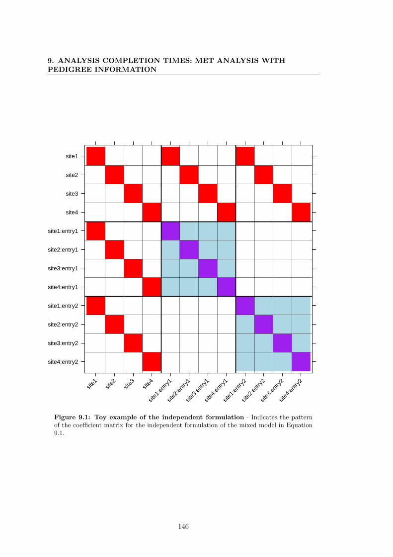
9. ANALYSIS COMPLETION TIMES: MET ANALYSIS WITHPEDIGREE INFORMATION
site4:entry2
site3:entry2
site2:entry2
site1:entry2
site4:entry1
site3:entry1
site2:entry1
site1:entry1
site4
site3
site2
site1
site1
site2
site3
site4
site1
:ent
ry1
site2
:ent
ry1
site3
:ent
ry1
site4
:ent
ry1
site1
:ent
ry2
site2
:ent
ry2
site3
:ent
ry2
site4
:ent
ry2
Figure 9.1: Toy example of the independent formulation - Indicates the patternof the coefficient matrix for the independent formulation of the mixed model in Equation9.1.
146
9.2 Computation background
9.2.2 Dependent formulation
Thompson et al. (2003) provided a different formulation to reduce computational loads.
In their formulation of the model in Equation 9.1, they first consider the partitioning
of the vector ug as ug = (ug1,ug2) which leads to,[ug1
ug2
]=
[Λ1 ⊗ ImΛ2 ⊗ Im
]f +
[δ1
δ2
](9.4)
where the elements of δ1 are all non-zero, but all the elements of δ2 are zero. Λ1 and
Λ2 are t1 × k and t2 × k matrices of loadings partitioned within ug. Also note that
t1 + t2 = t. This main model gives rise to two simplified forms, which enables some or
all of the specific variances to be zero:
1. t1 = t and t2 = 0, which assumes that all specific variance are non-zero
2. t1 = 0 and t2 = t, which assumes that all specific variance are zero
The model that Thompson et al. (2003) consider for a series of t trials and m entries
is of the form,
y = Xτ +Zcuc + e (9.5)
where y, τ andX are as previously stated; Zc = [Zf2, Zg1], whereZf2 = Zg2(Λ⊗Im);
uc = (f , ug1). The dependent formulation considered in this section, is the case where
there are no zero ψ, which results in: uc = (f , ug) and Zc = [0, Zg].
The variance assumptions are as previously stated, so that
var (uc) = Gc ⊗ Im =
[Ik ΛT
Λ ΛΛT +ψ
]⊗ Im
The MME for the model in Equation 9.5 are,[XTR−1X XTR−1Zc
ZcTR−1X Zc
TR−1Zc +Gc−1 ⊗ Im
][τ
uc
]=
[XTR−1y
ZcTR−1y
](9.6)
147
9. ANALYSIS COMPLETION TIMES: MET ANALYSIS WITHPEDIGREE INFORMATION
where Gc−1 = [
Ik + ΛTψ−1Λ −ΛTψ−1
−ψ−1Λ ψ−1
]
Similar to the independent formulation the coefficient matrix in Equation 9.6 is split
into two parts, data and variance: XTR−1X 0 XTR−1Zg
0 0 0
ZgTR−1X 0 Zg
TR−1Zg
+ 0 0 0
0 (Ik + ΛTψ−1Λ)⊗ Im −ΛTψ−1 ⊗ Im0 −ψ−1Λ⊗ Im ψ−1 ⊗ Im
9.2.2.1 Toy Example
The same toy data set described in the previous section, was analysed using the de-
pendent formulation in Equation 9.5. The model included a fixed effect for each site
(no overall mean), random entry effects for each site and a random factor score for
each entry. The coefficient matrix, C of the MME was then derived using Equation
9.6, see Fig. 9.2. Similarly to the previous section, the pattern of C was observed by
replacing actual values with colour. The labels of rows and columns in Fig. 9.2 are
“site1, .... , site4” - indicating site fixed effects, “fac:entry1” - random factor score
for entry 1,“site1:entry1, .... , site4:entry1” - indicating the random effects for entry
1 at each site, “fac:entry2” - random factor score for entry 2, and “site1:entry2, .... ,
site4:entry2” - indicating the random effects for entry 2 at each site.
148
9.2 Computation background
site4:entry2
site3:entry2
site2:entry2
site1:entry2
fac:entry2
site4:entry1
site3:entry1
site2:entry1
site1:entry1
fac:entry1
site4
site3
site2
site1
site1
site2
site3
site4
fac:e
ntry
1
site1
:ent
ry1
site2
:ent
ry1
site3
:ent
ry1
site4
:ent
ry1
fac:e
ntry
2
site1
:ent
ry2
site2
:ent
ry2
site3
:ent
ry2
site4
:ent
ry2
Figure 9.2: Toy example of dependent formulation - Indicates the pattern of thecoefficient matrix for the dependent formulation of the model in Equation 9.5.
149

9. ANALYSIS COMPLETION TIMES: MET ANALYSIS WITHPEDIGREE INFORMATION
9.2.3 Reduced rank version - dependent formulation
The fully reduced rank (RR) formulation of Thompson et al. (2003) with an additional
explicit term to accommodate specific variances is considered. This will be referred to
as the RR+diag model. The RR+diag model is written as,
y = Xτ +Zcuc +Zgδ + e (9.7)
where uc = f and Zc = Zf = Zg(Λ ⊗ Im). Note that this is the case of t1 = 0 and
t2 = t in Section 9.2.2.
The MME for the model in Equation 9.7 are, XTR−1X XTR−1Zf XTR−1Zg
ZfTR−1X Zf
TR−1Zf + Ik ⊗ Im ZfTR−1Zg
ZgTR−1X Zg
TR−1Zf ZgTR−1Zg +ψ−1 ⊗ Im
τfδ
=
XTR−1y
ZfTR−1y
ZgTR−1y
(9.8)
Similarly to the independent formulation the coefficient matrix in Equation 9.8 is split
into two parts, data and variance: XTR−1X XTR−1Zf XTR−1Zg
ZfTR−1X Zf
TR−1Zf ZfTR−1Zg
ZgTR−1X Zg
TR−1Zf ZgTR−1Zg
+ 0 0 0
0 Ik ⊗ Im 0
0 0 ψ−1 ⊗ Im
9.2.3.1 Toy Example
The same toy data set, and process was utilized for the RR+diag version of the de-
pendent formulation in Equation 9.7. The model included a fixed effect for each site
(no overall mean), a random factor score for each entry and random entry effect for
each site. Note that in contrast to Sections 9.2.2.1 and 9.2.1.1 the latter represent the
150

9.2 Computation background
“residual” entry effects at each site, ie. δ rather than the total entry effect ie. ug.
The coefficient matrix, C of the MME was then derived using Equation 9.8, see Fig.
9.3. The pattern of C was observed by replacing actual values with colour. The labels
of rows and columns in Fig. 9.3 are “site1, .... , site4” - indicating site fixed effects,
“fac:entry1” - random factor score for entry 1,“site1:entry1, .... , site4:entry1” - indi-
cating the random effects for entry 1 at each site, “fac:entry2” - random factor score for
entry 2 and “site1:entry2, .... , site4:entry2” - indicating the random effects for entry 2
at each site.
151

9. ANALYSIS COMPLETION TIMES: MET ANALYSIS WITHPEDIGREE INFORMATION
site4:entry2
site3:entry2
site2:entry2
site1:entry2
fac:entry2
site4:entry1
site3:entry1
site2:entry1
site1:entry1
fac:entry1
site4
site3
site2
site1
site1
site2
site3
site4
fac:e
ntry
1
site1
:ent
ry1
site2
:ent
ry1
site3
:ent
ry1
site4
:ent
ry1
fac:e
ntry
2
site1
:ent
ry2
site2
:ent
ry2
site3
:ent
ry2
site4
:ent
ry2
Figure 9.3: Toy example of RR version of dependent formulation - Indicates thesparsity pattern of the coefficient matrix for the RR+diag formulation of the mixed modelin Equation 9.7.
152

9.2 Computation background
9.2.4 Absorption
Solving the MME requires the inversion of the coefficient matrix (C). This is achieved
using the process of absorption (or Gaussian elimination) and back-substitution. In
this section the process of absorption is detailed.
After the ordering of the coefficient matrix, C, ASReml-R undertakes absorption
sequentially, that is a single row at a time beginning from the bottom line, and con-
tinuing upwards. Given a set of MME, the coefficient matrix can be written and then
subsequently partitioned as:
C =
C11 C12 C13 · · · C1,(N−1) C1N
C21 C21 C23 · · · C2,(N−1)
......
......
... · · ·...
C(N−1),1
......
.... . . C(N−1),N
CN1 · · · · · · · · · · · · CNN
=
[C11 c1N
cT1N cNN
]
where N is the order of the coefficient matrix C. C11 is the top portion of C, a matrix
of dimensions (N − 1) × (N − 1); c1N and cT1N are the far right column and bottom
row of the matrix C respectively. c1N is a vector of length (N − 1). cNN is a scalar,
and is often referred to as the pivot (Gilmour et al., 1995).
Given C above, the process of absorption involves forming the updated matrix,
C? = C11 − c1NcT1N/cNN (9.9)
where C? is an (N − 1) × (N − 1) matrix. The absorption process is then applied to
C? to form an updated matrix of dimension (N − 2)× (N − 2) and so on.
9.2.5 Sparsity and ordering
The coefficient matrix, C of the MME is often sparse, that is, it contains many zero-
valued elements. The computational burden of the absorption process can be reduced
if this is taken into consideration (Gilmour et al., 1995, Thompson, 2009). Specifically,
153

9. ANALYSIS COMPLETION TIMES: MET ANALYSIS WITHPEDIGREE INFORMATION
computing time is reduced by eliminating operations on the zero elements. Since ab-
sorption is a sequential process, it is not only the sparsity of C but also the updated
matrices (of the form in Equation 9.9) that is important. The latter is often influ-
enced by the ordering of the equations. A good ordering is one that maintains sparsity,
that is, minimises fill-in during the absorption process (Meyer, 1989, Thompson, 2009).
Gilmour et al. (1995) summarises the point in their statement “Assuming we avoid
multiplication by zero and that cT1N (Equation 9.9) has ni non-zero values, the number
of multiplications is (ni +1)(ni +2)/2. Thus operations can be avoided by ordering the
equations to minimize ni at each stage” (pg 1449).
In terms of the fitting of FA models, the ordering of the equations in the MME
corresponding to the genetic effects is a key determinant of computing time. This is
most easily seen by considering the toy example. The sparsity pattern of C, for the
dependent formulation (Fig. 9.2) is such that the section corresponding to the genetic
effects (10 × 10 partition in the bottom right hand corner) is relatively sparse. Now
consider a single absorption using two different orderings:
• The C matrix is ordered as in Fig. 9.2
• The C matrix is ordered as above but fac:entry2 is moved to the last row and
column
For both these scenarios the sparsity pattern of the updated matrix (C?) after
absorption is obtained. In the first ordering scenario the absorption of site4:entry2
resulted in a sparse updated matrix (Fig. 9.4). However in the second scenario, the
absorption of a factor score, ie. fac:entry2 resulted in substantial fill-in (Fig. 9.5). As
a result, there will be a greater number of computations to be carried out for scenario
two, which would be computationally intensive in comparison to scenario one.
The sparsity pattern of C for the independent formulation (Fig. 9.1) is such that
the section corresponding to the genetic effects (8 × 8 partition in the bottom right
hand corner) contains two dense sub-blocks. Thus C itself is less sparse than in the
dependent formulation and no re-ordering can improve the absorption process. Note
that the independent formulation was the original formulation in ASReml-R. It was
replaced by the dependent (also called the “sparse”) formulation of Thompson et al.
(2003) after this was shown to result in substantial time savings. This is the current
154
9.2 Computation background
site3:entry2
site2:entry2
site1:entry2
fac:entry2
site4:entry1
site3:entry1
site2:entry1
site1:entry1
fac:entry1
site4
site3
site2
site1
site1
site2
site3
site4
fac:e
ntry
1
site1
:ent
ry1
site2
:ent
ry1
site3
:ent
ry1
site4
:ent
ry1
fac:e
ntry
2
site1
:ent
ry2
site2
:ent
ry2
site3
:ent
ry2
Figure 9.4: Sparsity after absorption in a toy example of the dependent for-mulation with correct ordering - The updated coefficient matrix C?, indicating thefill in pattern resulting from the correct ordering of C. Black shading indicates non-zerocells and white indicates zero cells.
155
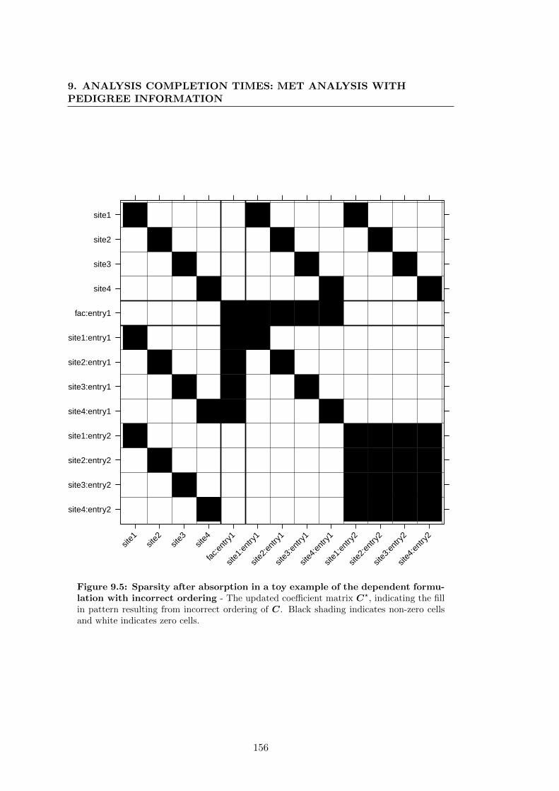
9. ANALYSIS COMPLETION TIMES: MET ANALYSIS WITHPEDIGREE INFORMATION
site4:entry2
site3:entry2
site2:entry2
site1:entry2
site4:entry1
site3:entry1
site2:entry1
site1:entry1
fac:entry1
site4
site3
site2
site1
site1
site2
site3
site4
fac:e
ntry
1
site1
:ent
ry1
site2
:ent
ry1
site3
:ent
ry1
site4
:ent
ry1
site1
:ent
ry2
site2
:ent
ry2
site3
:ent
ry2
site4
:ent
ry2
Figure 9.5: Sparsity after absorption in a toy example of the dependent formu-lation with incorrect ordering - The updated coefficient matrix C?, indicating the fillin pattern resulting from incorrect ordering of C. Black shading indicates non-zero cellsand white indicates zero cells.
156
9.2 Computation background
formulation implemented in ASRreml-R, and has been reported as resulting in a savings
of 50% of computational time when t = 17 and k = 3 and up to 90% when t = 62 and
k = 3 (Thompson et al., 2003, Thompson, 2009). A summary of the iteration times for
two data sets analyzed under independent and dependent formulations by Thompson
et al. (2003) were reproduced in Table 9.1.
Table 9.1: Time taken (in seconds) for completion of an iteration for independent anddependent formulations. This table has been reproduced from (Thompson et al., 2003)
AlgorithmDataset Model Dependent Independent (Smith et al., 2001b)
Lupins, p = 17 FA(1) 1.2 5.1Lupins, p = 17 FA(2) 2.2 5.5Lupins, p = 17 FA(3) 2.6 5.9Barley, p = 62 FA(1) 30 786Barley, p = 62 FA(2) 50 833Barley, p = 62 FA(3) 101 940
As discussed above it is vital with the dependent formulation that all site:entry
effects are absorbed prior to the factor scores. This means that the MME must be
re-ordered to allow this. Thompson et al. (2003) suggested that “A simple algorithm
would be to (i) count the non-zero elements in each row, (ii) absorb the row with
the least number of non-zero elements and update C, then repeat the process on the
updated C matrix” (pg 402). In terms of the genetic effects in the toy example (Fig.
9.4) this would result in the absorption of the rows associated with the site:entry effects
(each of the associated rows has only 3 non-zero elements) prior to the factor scores
(each of the associated rows has 5 non-zero elements). However, in real examples,
the non-genetic models are much more complex so that the ordering may not be as
clear-cut. The problem is exacerbated with the inclusion of pedigree information which
creates a far more dense set of equations for the site:entry effects. With these models it
is important to not only consider absorption of site:entry effects prior to factor scores
but also to order so that offspring are absorbed prior to parents. It is difficult to find
an ordering algorithm that can deal with such complexities and it is hypothesized that
currently in ASReml-R the inclusion of pedigree information in a MET analysis leads
to an inefficient ordering, resulting in factor scores being absorbed prior to site:entry
effects.
In an attempt to overcome this, the third formulation of the FA model, namely the
157
9. ANALYSIS COMPLETION TIMES: MET ANALYSIS WITHPEDIGREE INFORMATION
RR+diag formulation is considered. The sparsity pattern ofC for the toy example (Fig.
9.3) is slightly more dense than for the dependent formulation (Fig. 9.2). However in
this formulation the factor scores are “loaded” with data (i.e. there are more red cells
and no blue cells in Fig. 9.3 compared with Fig. 9.2) with the end result that the
number of non-zero elements in the rows corresponding to factor scores far exceeds
that for the rows corresponding to site:entry effects (9 compared with 3). Thus for
more complex models (including METs with pedigree information) it is, arguably, more
likely that the factor scores will be absorbed after the site:entry effects and hence the
computational efficiencies associated with sparsity will be exploited. This hypothesis
is examined empirically in the next section.
9.3 Example: Analysis completion times
9.3.1 The data set
In this section, the time required for the completion of a MET/FA analysis with and
without pedigree information is quantified. The complete CBWA canola MET data
set as described in Chapter 6 was used for the analyses conducted. From the CBWA
data set, four sub data sets of varying length (years) were created with corresponding
pedigree files, see summary in Table 9.2. Pedigree files were trimmed to contain only
entries (and parents of entries) present in the corresponding data file using the package
“Pedicure” (Butler, 2012) in R (R Development Core Team, 2012). Data subsets were
based on one to four years, and included the most recent growing season, 2011.
Table 9.2: Summary information on CBWA data subsets analyzed.
Data subsets Years Trials Number of records Entries Mums Dads
2011 1 10 5940 1084 235 3132011-2010 2 22 12444 1952 274 5662011-2009 3 35 17832 2533 302 7792011-2008 4 47 20928 2624 307 784
158
9.3 Example: Analysis completion times
9.3.2 Analysis
The spatial model for each trial was determined using the techniques outlined in Chap-
ter 7. These spatial models were retained for all subsequent analyses. Three stages
of models were fitted, the first assumed independence of entries, the second fitted ad-
ditive genetic effects only and the third fitted both additive and non-additive genetic
effects. For each stage of models, different forms of the genetic variance matrix were
considered, beginning with the diagonal model, followed by a factor analytic model
with k = 1 factors, fitted using the formulation described in Section 9.2.2 (denoted
FA(1)) and then the formulation described in Section 9.2.3 (denoted RR(1)+diag). In
doing so a step wise procedure was utilized to understand the cause of the extensive
time to completion observed for mixed model analysis with pedigree information.
9.3.3 Computation
Each of the following models were run in ASReml-R 3.0− 1 (library 3.0hj) on a Apple
Macintosh core 2.66GHz Intel Core i7 processor with 8GB RAM. The workspace was
set at a standard of 100e7 (or 800, 000, 000 bytes) for each of the models fitted. The
time (in seconds) required to complete the second iteration was obtained from the
difference between the times required for the second iteration and first iteration. The
time taken to complete the second iteration was used as an accurate representation for
time to analysis, as it excludes the initial setting up of design matrices that correspond
to the time taken for the completion of the first iteration.
9.3.4 Results & Discussion
The number of trials in the data sets increased from 10 in the one year data set to
47 in the four year data set (Table 9.3). There is almost a linear increase in the
number of entries for these respective data sets, increasing from 5940 to 20928. This
is approximately an increase of 3.5 times. There was a small increase in comparison
for the number of mums and dads in the pedigree files, between the one and four year
data sets (Table 9.3).
159

9. ANALYSIS COMPLETION TIMES: MET ANALYSIS WITHPEDIGREE INFORMATION
Table 9.3: Sequence of models fitted for genetic variance structures.
Model number Model summary Additive Non-additive Total
1 ND none none diag2 NF none none FA(1)3 NR none none RR(1) + diag
4 DN diag none5 FN FA(1) none6 RN RR(1) + diag none7 DD diag diag8 FF FA(1) FA(1)9 RR RR(1) + diag RR(1) + diag
Model acronyms: diag = diagonal model, FA(1) = factor analytic model of order 1 fitted using the
formulation in Section 9.2.2 and RR(1)+diag = factor analytic model of order 1 fitted using the
formulation in Section 9.2.3
Considering the models without pedigree information (ND, NF and NR in Fig. 9.6),
these all took less than 1 minute for the completion of the second iteration for all data
sets. The inclusion of pedigree information and the modeling of additive genetic effects
(i.e models DN, FN, RN) resulted in substantial differences between models in terms
of the time taken for the completion of the second iteration. The time required for the
FN model ranged from 125.9 seconds for the one year data set, to 1522.1 seconds for
the four year data set. In comparison to RN models, the FN models were 4.9, 7.7, 10.3
and 12.9 times larger for the one to four year data sets respectively. For the models
that included additive and non-additive genetic effects (models DD, FF, RR) there
was a large increase in completion of second iteration times for FF and RR models.
Comparing the FN and FF models, there was an increase in magnitude of computation
of 4.8, 3.3, 2.6, 2.1 for the one to four year data sets. In comparison to the RR models,
the FF model was 2.4, 2.9, 3.1 and 3.3 times slower for the one to four year data sets.
160
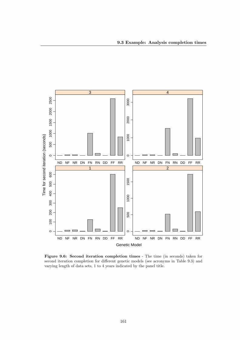
9.3 Example: Analysis completion times
Genetic Model
Tim
e fo
r se
cond
iter
atio
n (s
econ
ds)
010
020
030
040
050
060
0
ND NF NR DN FN RN DD FF RR
1
050
010
0015
00
ND NF NR DN FN RN DD FF RR
2
050
010
0015
0020
0025
00
ND NF NR DN FN RN DD FF RR
3
010
0020
0030
00
ND NF NR DN FN RN DD FF RR
4
Figure 9.6: Second iteration completion times - The time (in seconds) taken forsecond iteration completion for different genetic models (see acronyms in Table 9.3) andvarying length of data sets, 1 to 4 years indicated by the panel title.
161
9. ANALYSIS COMPLETION TIMES: MET ANALYSIS WITHPEDIGREE INFORMATION
It is evident that the inclusion of pedigree information in MET/FA analysis increases
the length of computation times for both FA(1) and RR(1)+diag models and this
increases with data set/pedigree length. However, the results indicate that the re-
parameterized RR(1)+diag model takes a third of the time as the FA(1) to complete
an iteration when pedigree information is included. This could be explained for the
toy example in Section 9.2.5, as the RR(1)+diag formulation loads up the factor rows
in the coefficient matrix, C, which prevents the absorption of the factor first and thus
avoids the resulting fill in effect.
9.3.5 Summary
During the course of this thesis, it was observed that the time for completion of
MET/FA models with pedigree information can be costly. This was investigated in this
chapter by firstly examining the possible model formulations available in ASRreml-R
followed by quantifying the actual times required for the completion of this analysis for
a real plant breeding data set. It is possible that long computational times, could be
attributed to issues with ordering when pedigree information is included in the model.
The formulation proposed in Section 9.2.3 appears to offer a quicker alternative in terms
of computational time.
162
Chapter 10
General Discussion
10.1 Introduction
The aim of a plant breeding program is to produce new varieties that are superior to
those already in the market, in terms of traits of economic importance such as yield
and quality etc. As a result, the process of plant breeding involves the manipulation
of complex traits in unpredictable environments (Hammer et al., 2006). Testing plant
breeding entries for many traits across a range of environments is costly, and the results
can be problematic if there are large errors or entries rank differently across environ-
ments; hence, the success of a plant-breeding program is linked to the efficiency of
selection methods. The topics of correlated traits, ancestry and environments were
researched in this thesis with the aim of demonstrating how the utilization of this ad-
ditional information can be used to improve the efficiency of selection within a plant
breeding program. This chapter brings together the main aims and findings across
all the chapters and provides a discussion on how the results from such analysis can
be interpreted and utilized with respect to a breeding program aims/objectives and
outcomes.
163

10. GENERAL DISCUSSION
10.2 Correlated traits
The first half of the thesis focused on correlated traits. The motivation behind this
study was the fact that while selection is usually undertaken on several traits within
a breeding program, plant breeding programs rarely use multivariate methods or an
index of selection, which is commonplace in animal breeding programs (Comstock et al.,
1996, Piepho et al., 2008).
Using a plant survival data set for blackleg disease of canola, a bivariate linear mixed
model approach was proposed in which the two variables are the initial and final plant
survival counts. The literature review in Chapter 2 discussed how such counts can be
subject to different biological, environmental and genetic factors, and showed how the
bivariate framework is statistically more accurate in accommodating this. The value of
the bivariate method (Chapter 3) was the modeling of spatial variation for each trait,
trait based outlier detection, and estimation of correlations between genetic effects and
errors between the two traits. This method clearly demonstrated that each set of plant
counts should be treated as separate traits as is the case under a bivariate analysis.
In terms of efficiency of selection, the bivariate approach not only provided a more
detailed picture for selection for disease resistance but also a more accurate assessment
of the impact of disease resistance compared with the historical analysis of percentage
survival data. The use of correlated traits in a bivariate framework of analysis enabled
a two dimensional view of selection, and three sources of information for selection
namely emergence counts, maturity counts and percentage survival values. Thus under
a bivariate analysis it was possible to obtain insights into the outcome of the plant-
pathogen interaction from the beginning to the end of the season, that would otherwise
not be observed under the historical analysis.
Efficiency of selection for the bivariate approach was evaluated by determining the
improvements in accuracy of prediction afforded over the univariate approaches for the
plant survival data. Modest improvements were achieved in prediction accuracies in
the bivariate model for the (log) emergence and (log) maturity traits and also for the
difference (log maturity − log emergence). Further it was also demonstrated that if
selection was preferred on the “difference” trait (log maturity− log emergence), this still
164

10.2 Correlated traits
should be done with reference to emergence. Thus the bivariate analysis was preferred
over the univariate analyses for the traits emergence, maturity and the difference.
The bivariate analysis allowed for a correlation between entry effects between emer-
gence and maturity to be estimated. This enabled an insight into plant/pathogen
relationships on particularly how blackleg disease could impact on entry emergence,
which was ignored under the historical univariate analysis. Studies on blackleg disease
have long reported that the type of genetic resistance against blackleg disease infection
is based on the stage of plant growth (Ballinger and Salisbury, 1996, Light et al., 2011,
Rempel and Hall, 1996, Roy, 1984). This would have an impact on entry selection,
as selection for resistance against blackleg disease could be undertaken based on plant
survival counts at emergence and/or maturity plant stages of growth.
While plant breeding experiments are multivariate in nature, there are few stud-
ies addressing issues of multivariate analysis in plant breeding. Chapter 4 addresses
a subset of studies on multivariate selection in plant breeding trials based on covari-
ance analysis, which is the most common approach in the plant breeding literature to
analyze for a single trait while “adjusting” for the presence of another trait. This is
effectively the historical approach to analysis of blackleg plant survival values (Chapter
3). Chapter 4 also discussed the potential application of a bivariate approach to other
plant selection experiments, which preferentially use covariance analysis to adjust for
one trait in the presence of another. These experiments included disease resistance
and grain yield and a subset of QTL studies in the areas of disease resistance, grain
yield and protein content. The covariance approach was contrasted with the bivari-
ate approach and it was discussed why the bivariate method would be preferred over
covariance analysis methods.
Covariance analysis has several problems, as highlighted in the subset of studies
reviewed in Chapter 4: (i) the covariate is often a trait that is also of interest for
selection, which implies that it has its own genetic variance (ii) covariance adjustment
to a common level, generates unrealistic varieties that do not exist in the experiment or
the breeding population, and (iii) the assumption that the covariate should be measured
without any error, is nearly impossible in plant breeding experiments. For points (i)
and (ii), above, the bivariate analysis enables a two-dimensional view for selection
165
10. GENERAL DISCUSSION
based on the two traits, without the need for an adjustment. Thereby it is a more
flexible framework of analysis as both traits can be incorporated into the selection
process. For point (iii), however, the bivariate framework enables the modeling of
spatial error for each trait, which is effectively ignored under covariance analysis. In
terms of efficiency, the bivariate framework should improve the efficiency of selection
in plant breeding programs, as there is no need to adjust one trait for another. While
multivariate analysis is common animal breeding (Falconer, 1981), the application of
multivariate analysis to plant breeding is complicated by the nature of plant breeding
trials. Bivariate analysis of field trials, as described in Chapter 3, is a novel method for
the achievement for multiple trait selection objectives in plant breeding with widespread
applications in the areas of disease resistance, grain yield, and protein content, as well
as QTL studies Chapter 4.
10.3 Ancestry & Environments
The second half of the thesis focuses on the impact of environment on selection and
the combined use of ancestry and environments to improve efficiency of selection.
The literature review presented in Chapter 5 found that the inclusion of pedigree
information in plant breeding METs resulted in major improvements in BLUP-based
prediction methods from mixed model analysis. Yet, few studies in the current scientific
literature are based on applied plant breeding programs (the exceptions are (Beeck
et al., 2010) and (Cullis et al., 2010)). This could be the result of complexity in the
fitting of these models, issues with the interpretation of results within the context of
plant breeding objectives and also limited worked examples. The processes described
in Chapters 7 (spatial analysis (N-gen modeling) of trials with pedigree information)
and 8 (MET/FA analysis), addressed these issues. The motivating data set for these
chapters was obtained from Canola Breeders Western Australia Pty Ltd (see description
in Chapter 6), a breeding program which utilize METs and mixed model analysis with
pedigree information in their canola breeding program.
Of the subset of studies reviewed in Chapter 5 that included pedigree information
in mixed model analysis, the studies by Crossa et al. (2006) and Burgueno et al. (2007)
166

10.3 Ancestry & Environments
omitted the use of spatial models. Chapter 7 as result, focused on demonstrating why
spatial modeling of non-genetic variance is important, especially in terms of efficiency
within a plant breeding context. Chapter 7 illustrated on an individual sites basis
the spatial modeling process and demonstrated the importance of pedigree information
in the spatial modeling of trials. With respect to (p-rep) trials, the results indicated
that the inclusion of pedigree information in spatial analysis is especially important.
Pedigree relationships in plant breeding trials can be used to borrow information from
relatives, which aids in the explanation of entry performance. The results of Chapter 7
also indicated that base-line non-genetic modelling should always include pedigree infor-
mation for the determination of site-specific spatial models, as there may be differences
between spatial models and outliers identified as a result of pedigree information.
There is a high level of adoption of p-rep trial designs, especially for the testing of
early generation entries (Cullis et al., 2006). Such trials attempt to provide accurate
selection of entries, with limited replication, for commercialization and parents for
the next cycle of breeding. As a result, it is important to minimize error, such as
environmental heterogeneity. Environmental effects are common in all designed field
trials, and if not accounted for can lead to biased estimates of treatment effects (Basford
and Cooper, 1998). Hence spatial analysis (N-gen modeling) should be undertaken
as standard for plant breeding trial analysis. However, published research has not
addressed the benefits of including pedigree information in finding optimum spatial
models in p-rep trials. The estimation of genetic merit in breeding trials is critical
for the efficiency of plant breeding programs, and spatial mixed model analysis with
pedigree information provides an improvement in efficiency.
Chapter 8 completed this process of model fitting by demonstrating the MET/FA
genetic modeling of the trials in Chapter 7 as well as providing an interpretation of the
results.
A key motivation for the use of a MET/FA model with pedigree information is
the independent estimation of additive and non-additive genetic effects as well as an
estimate of GxE on these components. This study extended this area of research by
considering different summaries of total genetic variance based on inbreeding coefficients
of entry types. Total genetic variance was summarized in three ways: for the entire
167

10. GENERAL DISCUSSION
data set, hybrid entries only and non-hybrid entries only. Previous studies are based
on total genetic variance evaluated from the average of all the diagonal elements of the
relationship matrix (Beeck et al., 2010, Oakey et al., 2006, 2007, Crossa et al., 2006).
This was relevant for the majority of these studies, given that their data sets were
composed of a single ‘type’ of entry; that is either hybrid or non-hybrid, rather than a
combination of the two. The motivational data set from CBWA however, represents a
current trend in plant breeding programs producing entries for both hybrid and open
pollinated market segments - our data set indicates a 50:50 split of entries for these
market segments.
MET/FA analysis provides an estimate of the presence and magnitude of GxE.
The findings of Chapter 8 indicate that within a single year (growing season) there is
substantial GxE. GxE was shown to be a large factor for Crop Variety Testing trials
in Western Australian (Gilmour et al., 1996) and for canola across production zones
in southern Australia (Beeck et al., 2010, Cullis et al., 2010). While cross over GxE
has the potential to complicate varietal selection (Chapters 5 and 8), an understand-
ing of genotypic adaptation to heterogeneous environments (Fukai and Cooper, 1995)
(Chapter 5) would enable broad or specific adaption patterns to be exploited for selec-
tion. Hence the interpretation of entry performance across environments is critical in a
plant breeding context as it maintains genetic gain in selection and this translates into
breeding program efficiency.
The results of cluster analysis for additive, non-additive and total genetic corre-
lations between trials indicated strong association of GxE with environmental factors
such as rainfall, drought, and frost as well as the biotic factor blackleg disease incidence.
While the target environments in CBAs breeding program are diverse (Fig. 6.1), the
clustering analysis suggested two main types of environments and different adaptation
of entries to these environments. The first cluster group of environments comprised
dryland agricultural zones, predominantly Western Australian wheatbelt sites, which
were characterized by short growing seasons with winter dominated rainfall and sandy
soils, and the second cluster group consisted of long season, equi-seasonal rainfall on
clay loamy soils in the eastern states of Australia.
Of most importance in this chapter is the differentiation of total genetic variance for
168

10.3 Ancestry & Environments
hybrids as well as non-hybrids, and the study of the impact of GxE on these entry types.
The resulting clustering analysis for hybrid and non-hybrid entry types indicated similar
patterns of GxE to that of total genetic variance across all entry types. The clustering
for hybrid and non-hybrid entries indicated adaptation patterns associated with annual
rainfall and length of growing season. Regardless, this differentiation enabled an insight
to the impacts of GxE on the different entry segments. For example, the C-BLUPs of
hybrid entries indicated disagreement between the two main cluster groups (Fig. 8.6)
which may indicate that heterosis is effective in some environments and not others (Xu
and Zhu, 1999). This would not have been otherwise observed by taking the average
of the inbreeding coefficients of all entries within the data set. Hence it highlights
the impact of environment on entry performance for these two entry types and would
impact on selection decisions. This highlights the fact that environment may influence
variety performance differentially for hybrids and non-hybrids, which (if not recognised)
may have a significant effect on selection decisions.
In terms of selection decisions, this chapter also demonstrated how predictions can
be used alongside the interpretation of cluster groups (Table 8.11). For additive genetic
effects (non-hybrid entries only) and total genetic effects (hybrid and non-hybrid en-
tries) it was possible to then identify entries with regional adaptation, that is to either
a particular cluster group, or even overall adaptation to both cluster groups. Efficiency
in selection would result from the ability to tailor selection to target environments en-
countered within the breeding program. This chapter in particular demonstrates how
genetic gain can be maintained and even improved in terms of selection by account-
ing for GxE. GxE would otherwise complicate selection and even mask genetic gain
impacting negatively on selection efficiency.
It is interesting to note that the cluster analysis for non-additive effects could be
explained by the presence or absence of blackleg disease at the trial sites. The challenge
to plant breeders is to exploit these non-heritable effects, as some may be due to epistasis
which can be fixed in inbred lines through crossing and recombination.
During the study of the MET/FA framework with pedigree information in Chapter
8, it was found that the time to complete these analyses was a potential limitation to
practical use in a commercial breeding program. As a result Chapter 9 researched the
169
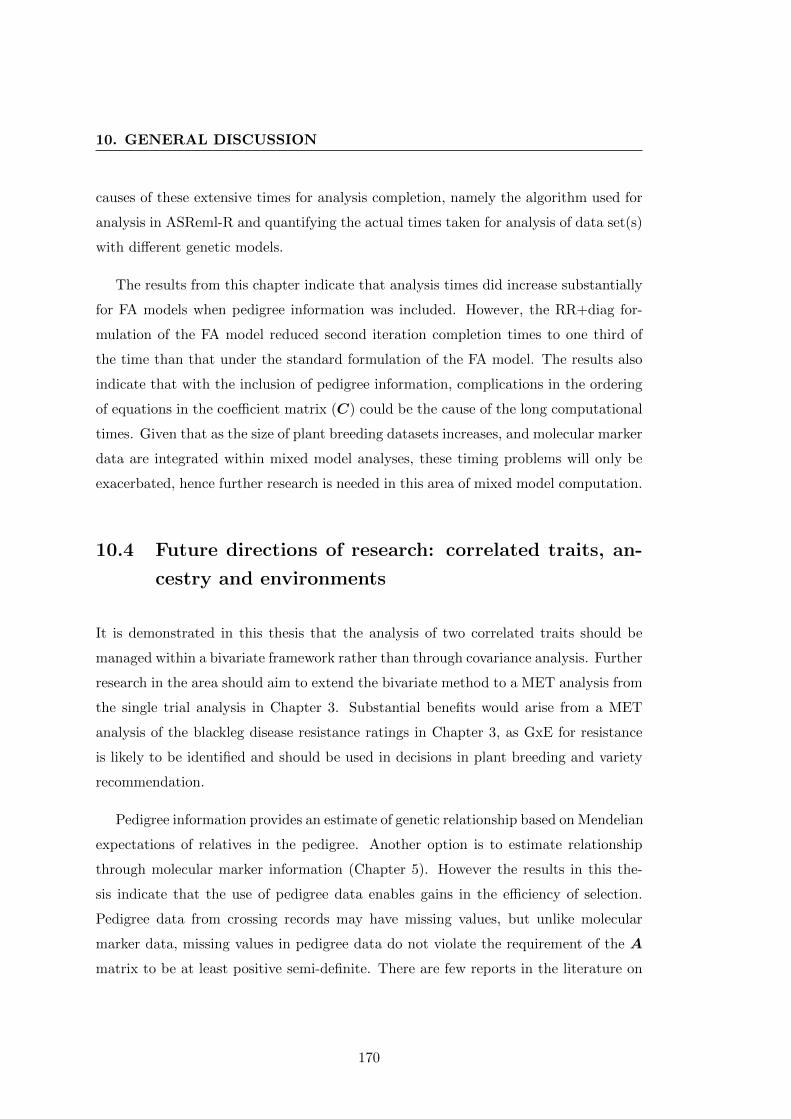
10. GENERAL DISCUSSION
causes of these extensive times for analysis completion, namely the algorithm used for
analysis in ASReml-R and quantifying the actual times taken for analysis of data set(s)
with different genetic models.
The results from this chapter indicate that analysis times did increase substantially
for FA models when pedigree information was included. However, the RR+diag for-
mulation of the FA model reduced second iteration completion times to one third of
the time than that under the standard formulation of the FA model. The results also
indicate that with the inclusion of pedigree information, complications in the ordering
of equations in the coefficient matrix (C) could be the cause of the long computational
times. Given that as the size of plant breeding datasets increases, and molecular marker
data are integrated within mixed model analyses, these timing problems will only be
exacerbated, hence further research is needed in this area of mixed model computation.
10.4 Future directions of research: correlated traits, an-
cestry and environments
It is demonstrated in this thesis that the analysis of two correlated traits should be
managed within a bivariate framework rather than through covariance analysis. Further
research in the area should aim to extend the bivariate method to a MET analysis from
the single trial analysis in Chapter 3. Substantial benefits would arise from a MET
analysis of the blackleg disease resistance ratings in Chapter 3, as GxE for resistance
is likely to be identified and should be used in decisions in plant breeding and variety
recommendation.
Pedigree information provides an estimate of genetic relationship based on Mendelian
expectations of relatives in the pedigree. Another option is to estimate relationship
through molecular marker information (Chapter 5). However the results in this the-
sis indicate that the use of pedigree data enables gains in the efficiency of selection.
Pedigree data from crossing records may have missing values, but unlike molecular
marker data, missing values in pedigree data do not violate the requirement of the A
matrix to be at least positive semi-definite. There are few reports in the literature on
170
10.5 Conclusion
the practical application of molecular marker data for estimation of genetic relation-
ships. Pedigree-based information can be as efficient as molecular marker information
to predict genetic effects (Mrode and Thompson, 2005, Maenhout et al., 2009). Further
there could be issues with the cost of molecular markers. Pedigree records are available
within plant breeding data bases, though it needs to be electronically accessible and
well managed in a database. Nevertheless the benefits of such information for a plant
breeding program makes this worth pursuing as it can result in efficiency of selection
within a plant breeding program, for very little added cost.
10.5 Conclusion
Statistical models in plant breeding programs aim to model the gene to phenotype
relationship (Cooper et al., 2005). This thesis examines how this can be improved with
the inclusion of information from correlated traits, ancestry and environments. This
thesis dealt with the efficiency of selection for the traits disease resistance and grain
yield. However it can be extended to a majority of crop production traits. It is hoped
that the efficiency gains demonstrated in this thesis will lead to greater adoption of
these methodologies in plant breeding programs.
171

10. GENERAL DISCUSSION
172

Appendices
173


Appendix A
Published paper based on
Chapter 3
175

A bivariate mixed model approach for the analysis of plantsurvival data
Aanandini Ganesalingam • Alison B. Smith •
Cameron P. Beeck • Wallace A. Cowling •
Robin Thompson • Brian R. Cullis
Received: 23 September 2011 / Accepted: 21 August 2012 / Published online: 30 August 2012
� Springer Science+Business Media B.V. 2012
Abstract Disease resistance is often measured as
plant survival, which involves taking multiple counts
of plants before and after disease incidence. Often,
survival data are analyzed by forming a single derived
variable, namely final counts expressed as a percent-
age of initial counts. In this study we propose a
bivariate linear mixed model approach in which the
two variables are the initial and final counts. This
approach is demonstrated using data from nine
blackleg disease nurseries in the 2009 growing season
in Australia. Replicated experiments were grown at
each nursery with a mixture of commercial Australian
canola cultivars and breeding lines (collectively called
‘entries’) being tested. Plant survival was determined
by counting all the seedlings at emergence and then
recounting the number surviving at maturity in each
plot. The counts were considered as two ‘traits’, which
were log transformed prior to a bivariate linear mixed
model analysis. Each trait had different error vari-
ances, spatial components (both local and global) and
outliers. The variance of entry effects was non-zero for
both traits at all locations. The correlation of entry
effects between the traits ranged from 0.218 to 0.935
across locations. Best Linear Unbiased Predictors
(BLUPs) of entry effects at both sampling times
provided three possible indices for selection: (log)
counts at emergence, (log) counts at maturity and the
difference between these two which could be expon-
entiated to provide percentage survival values. Thus
the bivariate mixed model approach for the analysis of
A. Ganesalingam (&) � A. B. Smith � C. P. Beeck
School of Plant Biology M084, The University of Western
Australia, 35 Stirling Highway, Crawley, WA 6009,
Australia
e-mail: [email protected]
A. B. Smith � B. R. Cullis
School of Mathematics and Applied Statistics, Faculty
of Informatics, University of Wollongong, Wollongong,
NSW, Australia
C. P. Beeck � W. A. Cowling
Canola Breeders Western Australia Pty Ltd, South Perth,
WA, Australia
W. A. Cowling
The UWA Institute of Agriculture, The University
of Western Australia, Crawley, WA, Australia
R. Thompson
Rothamsted Research, Harpenden, UK
R. Thompson
Queen Mary University of London, London, UK
B. R. Cullis
Division of Mathematics, Informatics and Statistics,
CSIRO, Canberra, ACT, Australia
123
Euphytica (2013) 190:371–383
DOI 10.1007/s10681-012-0791-0
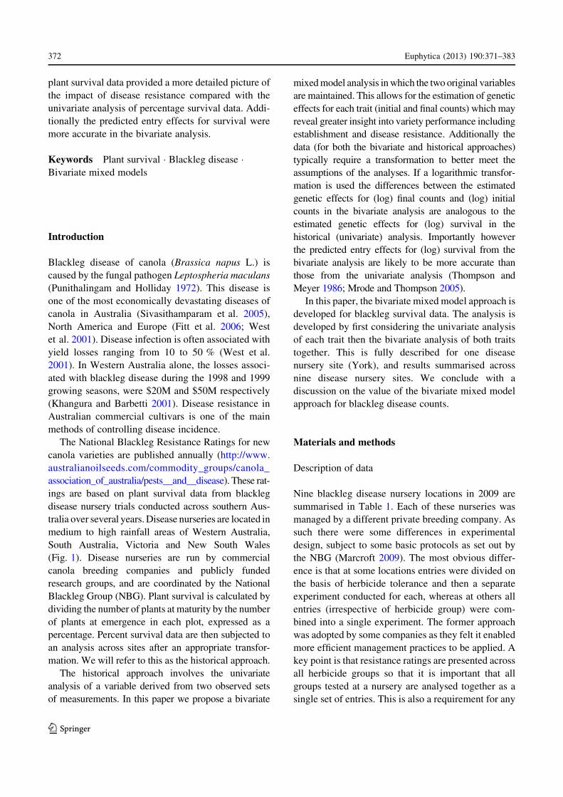
plant survival data provided a more detailed picture of
the impact of disease resistance compared with the
univariate analysis of percentage survival data. Addi-
tionally the predicted entry effects for survival were
more accurate in the bivariate analysis.
Keywords Plant survival � Blackleg disease �Bivariate mixed models
Introduction
Blackleg disease of canola (Brassica napus L.) is
caused by the fungal pathogen Leptospheria maculans
(Punithalingam and Holliday 1972). This disease is
one of the most economically devastating diseases of
canola in Australia (Sivasithamparam et al. 2005),
North America and Europe (Fitt et al. 2006; West
et al. 2001). Disease infection is often associated with
yield losses ranging from 10 to 50 % (West et al.
2001). In Western Australia alone, the losses associ-
ated with blackleg disease during the 1998 and 1999
growing seasons, were $20M and $50M respectively
(Khangura and Barbetti 2001). Disease resistance in
Australian commercial cultivars is one of the main
methods of controlling disease incidence.
The National Blackleg Resistance Ratings for new
canola varieties are published annually (http://www.
australianoilseeds.com/commodity_groups/canola_
association_of_australia/pests__and__disease). These rat-
ings are based on plant survival data from blackleg
disease nursery trials conducted across southern Aus-
tralia over several years. Disease nurseries are located in
medium to high rainfall areas of Western Australia,
South Australia, Victoria and New South Wales
(Fig. 1). Disease nurseries are run by commercial
canola breeding companies and publicly funded
research groups, and are coordinated by the National
Blackleg Group (NBG). Plant survival is calculated by
dividing the number of plants at maturity by the number
of plants at emergence in each plot, expressed as a
percentage. Percent survival data are then subjected to
an analysis across sites after an appropriate transfor-
mation. We will refer to this as the historical approach.
The historical approach involves the univariate
analysis of a variable derived from two observed sets
of measurements. In this paper we propose a bivariate
mixed model analysis in which the two original variables
are maintained. This allows for the estimation of genetic
effects for each trait (initial and final counts) which may
reveal greater insight into variety performance including
establishment and disease resistance. Additionally the
data (for both the bivariate and historical approaches)
typically require a transformation to better meet the
assumptions of the analyses. If a logarithmic transfor-
mation is used the differences between the estimated
genetic effects for (log) final counts and (log) initial
counts in the bivariate analysis are analogous to the
estimated genetic effects for (log) survival in the
historical (univariate) analysis. Importantly however
the predicted entry effects for (log) survival from the
bivariate analysis are likely to be more accurate than
those from the univariate analysis (Thompson and
Meyer 1986; Mrode and Thompson 2005).
In this paper, the bivariate mixed model approach is
developed for blackleg survival data. The analysis is
developed by first considering the univariate analysis
of each trait then the bivariate analysis of both traits
together. This is fully described for one disease
nursery site (York), and results summarised across
nine disease nursery sites. We conclude with a
discussion on the value of the bivariate mixed model
approach for blackleg disease counts.
Materials and methods
Description of data
Nine blackleg disease nursery locations in 2009 are
summarised in Table 1. Each of these nurseries was
managed by a different private breeding company. As
such there were some differences in experimental
design, subject to some basic protocols as set out by
the NBG (Marcroft 2009). The most obvious differ-
ence is that at some locations entries were divided on
the basis of herbicide tolerance and then a separate
experiment conducted for each, whereas at others all
entries (irrespective of herbicide group) were com-
bined into a single experiment. The former approach
was adopted by some companies as they felt it enabled
more efficient management practices to be applied. A
key point is that resistance ratings are presented across
all herbicide groups so that it is important that all
groups tested at a nursery are analysed together as a
single set of entries. This is also a requirement for any
372 Euphytica (2013) 190:371–383
123

multi-environment trial (MET) analysis as it ensures
that entry concurrence (commonality) is maximised
across locations within a year.
High disease levels at each nursery were promoted
by growing entries on or with blackleg-infested
stubble from the previous season. The stubble source
at each disease nursery is given in Table 2. Disease
nurseries were only included in the data set if the
susceptible control entry, Karoo had less than 30 %
survival (Marcroft 2009). Standard management prac-
tices were followed across all disease nurseries and are
set out in the protocols determined by the NBG
(Marcroft 2009). It is current NBG protocol to omit
plots with less than 20 emergence counts due to poor
Fig. 1 Geographic
locations of nine blackleg
(Leptospheria maculans)
disease nurseries across
southern Australia during
the 2009 growing season
Table 1 Description of
blackleg disease nursery
experiments during the 2009
growing season
Each location is composed of
one or more experiments based
on herbicide type. The number
of entries, columns, rows and
blocks are listed for each
experiment in this data set
Conv conventional, Clclearfield�, TT triazine
tolerant, RR round up ready�
Location Experiment Herbicide type Entries Columns Rows Blocks
Bakers Hill BH Conv, Cl, TT 57 3 57 3
Bordertown BT1 Cl 13 3 13 3
BT2 TT 28 6 14 3
BT3 Conv 24 6 12 3
BT4 Conv, Cl, TT 33 3 33 3
Clear Lake CL Conv, Cl, TT 18 4 20 4
Lake Bolac LB1 Conv, TT 24 12 8 3
LB2 RR 31 12 10 3
LB3 Conv, Cl, TT, RR 107 12 30 3
Nurcoung NU1 RR 24 12 8 3
NU2 Conv, Cl, TT, RR 107 12 30 3
Shenton Park SP Conv, Cl, TT 65 22 9 4
Wagga Wagga WA Conv, Cl, TT 74 15 16 3
Wonwondah WO Conv, TT 31 12 10 3
York YK Conv, TT 78 3 79 3
Euphytica (2013) 190:371–383 373
123

germination, and to truncate plots with greater than
100 % survival to 100 %. For the bivariate analysis
however, the data for all plots were retained.
All experiments in this data set were designed as
randomized complete block designs (RCB) with either
3 or 4 replicates and extra plots of controls. All
experiments were laid out as a rectangular array
indexed by rows and columns (Table 1). Sufficient
seed was sown by hand or machine to target 100
established plants per plot. The number of emerged
seedlings per plot was counted at 4–6 weeks after
sowing, and the number of surviving plants per plot
was counted when plants were mature, at the wind-
rowing stage.
Statistical methods
Univariate analysis
The first step in the bivariate analysis is to identify
appropriate spatial models for each trait, following the
spatial mixed model approach of Gilmour et al.
(1997). This is most readily achieved by conducting
a separate univariate analysis for each trait. The
univariate models are then incorporated into the
bivariate analysis.
We describe the approach for one disease nursery
(York) that comprises a single experiment (Table 1).
Let r and c be the number of rows and columns
respectively so that the total number of plots is given
by n = rc, m is the number of entries and b the number
of blocks in the RCB design. At York, n = 237 plots,
r = 79 rows, c = 3 columns, b = 3 blocks and
m = 78 entries (Table 1). Note, that there were extra
plots of the variety GT61 sown, as there was not
enough seed for the variety CBTM Mallee HTTM. The
data are ordered as rows within columns. The base line
univariate mixed model is developed for the data at
sampling time j, (j = 1, 2), where j corresponds to 1
for emergence counts and 2 for maturity counts, and is
given by:
yj ¼ Xsj þ Zvuvj þ Zbubj þ ej ð1Þ
where yj is the n 9 1 vector of data; sj is the vector of
fixed effects (in this case the overall site mean) with
associated design matrix X; uvj is the m 9 1 vector of
random entry effects with associated design matrix
Zv; ubj is the b 9 1 vector of random block effects
with associated design matrix Zb, and ej is the vector of
residuals ordered as per the data vector. There are no
sub-scripts associated with the design matrices since,
for the base-line model, they are the same for both
sampling times.
Entry effects are assumed to be independent with
variance r2v j and the block effects to be independent
with variance r2bj. This is written as var ðuvjÞ ¼ r2
v jIm
and var ðubjÞ ¼ r2bjIb where Im and Ib are identity
matrices of dimensions m 9 m and b 9 b respectively.
In terms of the errors, a separable autoregressive
process of order one (AR1) as proposed by (Gilmour
et al. 1997) was assumed. Thus we write var ðejÞ ¼Rj ¼ r2
j Rcj � Rrj; where rj2 is the error variance at
sampling time j;Rcj is a c 9 c correlation matrix for
trend in the column dimension and Rrj a r 9 r
correlation matrix for trend in the row dimension.
Each matrix is a function of a single autocorrelation
parameter qcj and qrj for the column and row
Table 2 Location based
details: state, stubble type,
number of experiments,
number of entries and average
plant counts at emergence
(eme) and maturity (mat) for
each of the 2009 blackleg
disease nurseries
Location State Stubble type Experiments Entries Average
Eme Mat
Bakers Hill WA Bravo TT 1 57 60 35
Bordertown SA Mixture 4 74 38 13
Clear Lake VIC 45Y77 1 18 50 33
Lake Bolac VIC ATR-Marlin 3 148 28 7
Nurcoung VIC ATR-Cobbler 2 128 50 15
Shenton Park WA CB Telfer 1 65 75 57
Wagga Wagga NSW Bravo TT 1 74 34 10
Wonwondah VIC AV-Garnet 1 31 37 14
York WA ATR-Cobbler 1 78 59 13
374 Euphytica (2013) 190:371–383
123

dimensions respectively. Experiments with four or
less columns, were assumed to have independence for
errors in the column dimension, so that Rcj ¼ Ic:
After the base line mixed model was fitted,
diagnostics were used to assess the adequacy of the
spatial models. These included plots of residuals
against row number for each column and a three
dimensional display of the sample variogram
(Gilmour et al. 1997). These diagnostics were used
to identify outliers and determine if additional fixed
and/or random terms were required in the model.
Nurseries with several experiments required a more
complex model. Here, the data vector included the
individual plot data combined across experiments,
ordered as rows within columns within experiments.
Thus the total number of plots is n ¼Ps
i¼1 ni where s
is the number of experiments and ni is the number of
plots in experiment i, i.e. (i ¼ 1; . . .; s). The base line
mixed model for sampling time j is given by:
yj ¼ Xsj þ Zvuvj þ Zeuej þ Zbubj þ ej ð2Þ
where uv is as previously defined (and m is the total
number of entries for the disease nursery location); ub
is now the b 9 1 vector of random block effects for
each experiment (so that b ¼Ps
i¼1 bi); ue is the s 9 1
vector of random experiment effects. The variance
assumptions for the random effects are now varðuvjÞ ¼
r2v j Im; varðuej
Þ ¼ r2e jIs and varðubj
Þ ¼ diagðrbji2IbiÞ:
Note, that the variance matrix for ubj is block diagonal
and implies a separate block variance for each
experiment. A separate spatial model for the errors
was allowed for each experiment, so: varðejÞ ¼ Rj ¼diagðRjiÞ where Rji ¼ ðr2
jiRcji � RrjiÞ: The use of
distinct spatial models and block variances for each
experiment was due to the fact that the experiments at
each nursery are physically separated from each other,
that is not adjoining.
The count data were first log-transformed before
analysis to approximate a Gaussian distribution with a
constant variance. Further, this transformation ensured
that the predicted counts were non-negative, which is
of biological significance to this analysis.
All models in this paper were fitted in ASReml-R
(Gilmour et al. 2009). This provided residual maxi-
mum likelihood (REML) estimates of the variance
parameters, (empirical) Best Linear Unbiased Esti-
mates (BLUEs) of the fixed effects and (empirical)
Best Linear Unbiased Predictions (BLUPs) of the
random effects.
Bivariate analysis
Having identified the appropriate spatial models from
the univariate analyses for the emergence and maturity
data, the bivariate analysis is then conducted. Again,
consider the simplest case of a nursery comprising a
single experiment. Let y ¼ ðy01; y02Þ0, be the combined
vector of data across sampling times. The mixed
model for the bivariate analysis is given by
y ¼ X�sþ Z�vuv þ Z�bub þ Z�ouo þ e ð3Þ
where uv ¼ ðu0v1u0v2Þ0
is the 2m 9 1 vector of random
entry effects and Z�v ¼ I2 � Zv is the associated design
matrix; ub ¼ ðu0b1; u0b2Þ0
is the 2b 9 1 vector of
random block effects and Zb� ¼ I2 � Zb is the asso-
ciated design matrix; e ¼ ðe01; e02Þ0
is the vector of
errors ordered as for the data vector. The vector of
fixed effects, s, includes an overall mean for each
sampling time and any other fixed effects as identified
in the spatial modelling (e.g. linear regression on
rows) from the univariate analyses. Any random
effects identified in the univariate analyses are
included in the vector uo.
The variance assumptions for the random entry
effects are,
varðuvÞ ¼ varuv1
uv2
� �
¼ r2v1
rv12 r2v2
� �
� Im ð4Þ
where rvj2 (j = 1, 2) are as previously defined (i.e. the
the variance of entry effects for each sampling time)
and rv12 is the covariance between the entry effects at
emergence and maturity. For ease of interpretation, we
converted the covariance between entry effects to a
correlation, i.e.
qv12 ¼rv12ffiffiffiffiffiffiffiffiffiffiffiffiffir2
v1r2v2
p ð5Þ
The variance assumptions for the block effects were
similar except the covariance between sampling times
was omitted if one or both block variances were small.
The variance assumptions for the vector uo were
chosen appropriately for the terms involved. For the
Euphytica (2013) 190:371–383 375
123

errors a separable spatial correlation model was
assumed, namely
varðeÞ ¼ vare1
e2
� �
¼ r21
r12 r22
� �
� Rc � Rr ð6Þ
where rj2 (j = 1, 2) is as previously defined (i.e. the
error variances for each sampling time) and r12 is the
covariance between the errors at emergence and
maturity. The latter accommodates the repeated mea-
sures nature of the data with two sampling times for
each plot. The error covariance was converted to a
correlation between the traits, as in Eq. 5. The (spatial)
correlation matrices Rc and Rr correspond to autore-
gressive processes of order one, that is, functions of
single parameters qc and qr respectively. The separa-
bility assumption implies that the same spatial corre-
lation parameters are applicable for both sampling
times. It may be desirable to allow different param-
eters, but such models are not yet available and are the
subject of current research.
After fitting this model the predicted entry means
(i.e. BLUPs of entry means) were obtained for each
sampling time. Let pjk denote the predicted entry mean
for entry k at sampling time j. These may be back-
transformed to the original scale as exp(pjk). The back-
transformed difference between the predicted means
for maturity and emergence is given by
expðp2k � p1kÞ ¼expðp2kÞexpðp1kÞ
ð7Þ
namely the ratio of maturity to emergence counts on
the back-transformed scale. This allows entries to be
assessed on the same basis as the historic approach,
namely in terms of percent survival.
Results
Univariate analysis
York disease nursery
Results of the univariate analyses are described in
detail for the York disease nursery in Western
Australia (Table 1; Fig. 1).
This experiment had three columns, so an AR1
spatial trend process was only modeled for the row
dimension in both trait models. After the model was
fitted, diagnostics including sample variograms and
residual plots were used to determine the adequacy of
spatial models. The plots for emergence (Fig. 2) showed
the existence of local spatial correlation in the row
direction (reflected in the smooth trend in the residual
plot), extraneous variation in the row direction (seen as
the up/down pattern in the variogram) and three outliers
(unusually low values on the residual plot). The outliers
were omitted from the subsequent analysis (i.e. the count
data were set as missing values). The extraneous
variation was accommodated by fitting random row
effects in the model, which improved the residual plot
and variogram (Fig. 3). The spatial correlation for trend
in the row direction was strong (0.72; see Table 3). In
contrast to the emergence analysis, there were no
extraneous effects in the maturity analysis. A single
outlier was detected and set to a missing value. The
spatial correlation in the row direction was much weaker
than for emergence (0.22; see Table 3).
The REML estimate of the variance of entry effects
for the emergence trait (0.400) was almost as large as
that for the maturity trait (0.511) (Table 4). The
variance component for blocks was very close to zero
(0.041 and 0.066 for the emergence and maturity
models respectively). The error variance component
for the emergence mixed model (0.382) was larger
than the maturity model (0.299) (Table 3).
All disease nurseries
Across all the disease nursery locations, there were
more outliers removed from the univariate emergence
model than the maturity model (Table 3).
The terms fitted to the mixed models for non-
stationary trend and extraneous variation differed for
each trait. There was more extraneous variation
present for emergence than maturity across all exper-
iments (Table 3). In 9 out of the total 15 experiments,
terms were required to encompass non-stationary
trend and extraneous variation for emergence and
maturity trait models.
In terms of stationary trend, there was variation
between trait models for column and row autocorre-
lation values (Table 3). Across all the emergence
mixed models, the largest column autocorrelation
value was 0.66 at BT2, and the largest row autocor-
relation value was 0.72 at YK (Table 3). For the
maturity mixed models, the largest column autocor-
relation value was 0.43 at NU1 and the largest row
376 Euphytica (2013) 190:371–383
123

autocorrelation value was 0.54 at NU1 (Table 3).
High autocorrelation values indicate the presence of
strong local trend in these experiments for the
respective trait model.
The REML estimates of variance of entry effects for
emergence and maturity were non-zero for all locations
(Table 4). Therefore, entries varied in emergence and
maturity traits at all disease nursery locations. Further-
more, the variance of entry effects for maturity was
substantially larger than that of emergence across all
experiments except Bakers Hill (Table 4).
Bivariate analysis
York disease nursery
For the bivariate analysis, the spatial terms from the
univariate trait mixed models were retained and the
bivariate model (Eq. 3) was fitted.
REML estimates of variance of entry effects for
emergence and maturity from the bivariate model
were close approximations of the variances of entry
effects obtained from the individual univariate mixed
models (Table 4). Similarly, the error variance com-
ponents from the bivariate model were close approx-
imations of the individual univariate analyses
(Table 3). The AR1 row correlation value under the
bivariate model was 0.362, which was close to the
average of the row correlations obtained under
the univariate trait analyses (Table 3).
The bivariate model included a correlation structure
for both the entry effects and the errors. The estimated
correlation of entry effects between the traits at York
was 0.71 and the correlation between trait errors was
0.59. The high correlation of entry effects demon-
strates an agreement between entry rankings for both
traits and the high error correlation reflects the impact
of the repeated measures nature of the data.
Fig. 2 Initial plot of residuals and sample variogram from the univariate emergence model at the York disease nursery
Euphytica (2013) 190:371–383 377
123

After fitting the bivariate model, BLUPs of entry
means at emergence and maturity for each experiment
were used to produce two plots. In the first, entry
means at maturity were plotted against entry means at
emergence (Fig. 4). In the second, the difference
between BLUPs of entry means for emergence and
maturity were plotted against the BLUPs of entry
means at emergence (Fig. 5). The difference between
the predicted entry means for emergence and maturity
corresponded to the percent survival scale of the
historical approach, when back-transformed (see
Eq. 7).
The maturity versus emergence plot showed large
variation in emergence of entries at York, from 10 to
100 plant counts (Fig. 4). The majority of entries
were clustered towards the centre of the graph, with
emergence counts between 20 and 50 and maturity
counts between 5 and 20. A regression line of
maturity against emergence, which is implicit in the
bivariate variance structure for the entry effects was
drawn in Fig. 4. This corresponds to the regression
of the true entry effects for maturity (i.e. uv2) on the
true entry effects for emergence (i.e. uv1). The slope is
given by
b ¼ qv12 �
ffiffiffiffiffiffiffir2
v2
r2v1
s
ð8Þ
The slope for York was 0.84, which indicates a strong
linear relationship between maturity and emergence
counts at this disease nursery location.
The percent survival versus emergence plot showed
that the control entry Surpass501TT had a very low
emergence count, with less than 20 plant counts, but an
average percentage survival value of 25 % (Fig. 5).
The highly resistant entry Hyola50 had average
emergence, but the highest percentage survival value
at 65 %. The entry 46Y20(J) had the highest plant
Fig. 3 Plot of residuals and sample variogram from the univariate emergence model at the York disease nursery after the addition of a
random row component and removal of outliers
378 Euphytica (2013) 190:371–383
123

emergence and maturity counts (Fig. 4) but average
percentage survival value of 25 % (Fig. 5).
All disease nurseries
In contrast to the York disease nursery, which had a
high correlation of entry effects between traits, the Lake
Bolac disease nursery had the lowest correlation of
entry effects between traits (Table 4). At Lake Bolac,
there was little agreement between entry rankings
across traits (Fig. 6). The slope of the regression line of
entry effects for maturity on emergence at this site was
0.49, which indicated weak linear relationship when
compared to York, which had a slope of 0.84.
Table 3 Spatial modelling in univariate analyses of emergence
(eme) and maturity (mat) trait data for each experiment: terms
added for global trend or extraneous variation, REML
estimates of error variance, REML estimates of autocorrelation
parameters (for columns and rows, where fitted) and number of
outliers removed
Expt Global trend & extraneous variation termsa Error variance Autocorrelation Number of outliers
Eme Mat Eme Mat Column Row Eme Mat
Eme Mat Eme Mat
BH rdRow 0.040 0.317 0.19 -0.03 1
BT1 0.102 0.150 -0.02 -0.33
BT2 0.062 0.410 0.66 0.26 0.03 0.35
BT3 0.265 0.261 0.6 0.42 -0.13 -0.1
BT4 0.136 0.191 -0.07 0.13 1 1
CL 0.017 0.064 0 0.26 1
LB1 rd(R) & rd(C) 0.078 0.26 -0.06 0.01 0.05 0.12 1
LB2 rd(R) & rd(C) 0.098 0.291 0.09 0.05 -0.07 0.04
LB3 rd(R) & rd(C) 0.160 0.283 0.01 0.04 0.01 0.04 1
NU1 0.169 0.089 0.23 0.43 0.39 0.54 1
NU2 rd(R) & rd(C) 0.183 0.111 0.09 0.35 0.12 0.16 3 4
SP lin(R) 0.015 0.054 0.02 -0.17 -0.05 0.17 2 2
WG rd(R) & rd(C) lin(C) 0.029 0.265 0.24 0.28 2
WO rd(R) & rd(C) 0.163 0.031 0.16 0.03 -0.13 -0.07
YK rd(R) 0.382 0.299 0.72 0.22 3 1
a lin(R) and lin(C) indicates a fixed linear regression on row or column number; rd(R) and rd(C) indicate random row and column
components
Table 4 REML estimates of
entry variance from univariate
trait model and bivariate model
at each disease nursery location
The correlation between entry
effects from the bivariate
model is also shown
Location Univariate Bivariate
Eme Mat Eme Mat Correlation
Bakers Hill 0.108 0.127 0.109 0.131 0.68
Bordertown 0.112 0.744 0.110 0.748 0.24
Clear Lake 0.042 0.232 0.047 0.259 0.68
Lake Bolac 0.124 0.622 0.126 0.629 0.22
Nurcoung 0.079 0.489 0.075 0.485 0.25
Shenton Park 0.191 0.657 0.194 0.636 0.94
Wagga Wagga 0.053 0.768 0.053 0.765 0.73
Wonwondah 0.033 0.687 0.034 0.691 0.73
York 0.400 0.511 0.354 0.493 0.71
Euphytica (2013) 190:371–383 379
123

The REML estimates of the variance of entry
effects for emergence and maturity at all sites were
similar to the approximations obtained from the
individual trait univariate analyses (Table 4). The
correlation of entry effects between the two traits
averaged 0.57 (range 0.22–0.94) across the nine
disease nursery locations.
Accuracy comparisons
As noted in the introduction one of the main advan-
tages in using a bivariate analysis is that it increases
the accuracy of predictions. The accuracy of a
prediction for a variety is defined here as the square
of the correlation between the true and predicted effect
for that variety. It can be computed using the estimated
genetic variance for the trait concerned and the
prediction error variance for the variety following
Mrode and Thompson (2005). In this paper the key
accuracy comparison is in terms of survival rates.
These accuracy values have been calculated for each
variety for each disease nursery from both the
bivariate analysis of (log) initial and (log) final counts
and the univariate analysis of the difference. To ensure
a fair comparison the estimates of genetic and
non-genetic variances (including block and error
variances) were held constant between the two
Emergence
Mat
urity
1
2
3
4
2.5 3.0 3.5 4.0 4.5 5.0
Surpass501TTHyola5046Y20(J)
10 20 30 40 50 60 70 80
10
20
30
40
50
60
7080
Fig. 4 Predicted entry means at emergence plotted against
predicted entry means at maturity from the bivariate model for
the disease nursery at York. A regression line of maturity against
emergence was included, with the slope having a value of 0.84.
The axes are on a log scale (as for the analysis) with the back-
transformed scale (i.e. plant counts) shown inside each axis
Emergence
Mat
urity
− E
mer
genc
e
−2.5
−2.0
−1.5
−1.0
−0.5
2.5 3.0 3.5 4.0 4.5 5.0
Surpass501TTHyola5046Y20(J)
10 20 30 40 50 60 70 80
10
20
30
40
50
60
70
Fig. 5 The difference between predicted entry means at
maturity and emergence (corresponds to percentage survival
when back transformed, these values are shown on the inside of
the y-axis) plotted against predicted entry means at emergence
from the bivariate model for the disease nursery at York
Emergence
Mat
urity
1
2
3
4
2.5 3.0 3.5
Surpass501TTHyola5046Y20(J)
0504030201
10
20
30
40
50
60
7080
Fig. 6 Predicted entry means at emergence plotted against
predicted entry means at maturity from the bivariate model for
the disease nursery at Lake Bolac. A regression line of maturity
against emergence was included, with the slope having a value
of 0.49. The axes are on a log scale (as for the analysis) with the
back-transformed scale (i.e. plant counts) shown inside each
axis
380 Euphytica (2013) 190:371–383
123

approaches. Thus for Bakers Hill, for example, the
genetic variances for the bivariate analysis were
rv12 = 0.109 and rv2
2 = 0.131 for the emergence and
maturity traits respectively, with a genetic correlation
of qv12 = 0.68 (see Table 4) so that the genetic
variance for the univariate analysis of the difference
was constrained to be equal to rv12 ? rv2
2 - 2qv12 rv1
rv2 = 0.078. Non-genetic components were con-
strained in a similar manner. Additionally identical
sets of counts (namely the complete data after the
removal of the outliers described in Table 3) were
used to obtain both the bivariate and univariate
predictions. The accuracy of prediction from the
bivariate analysis was greater than that from the
univariate analysis for all varieties in all nurseries.
The average percentage gain for individual nurseries
ranged from 0.1 to 5.6 % with a mean of 1.1 % (see
Table 5). The gains were small for those nurseries
where the univariate accuracies were high (that is, near
the maximum possible value of 1.0), whereas more
substantial gains were observed for those nurseries
where the univariate accuracies were lower.
Discussion
In this article, a bivariate mixed model approach for
the analysis of plant survival data is described and
applied to data from nine Australian canola blackleg
disease nursery trials. The two traits (variables) in the
bivariate analysis are plant counts at emergence and
plant counts at maturity.
A valuable feature of the bivariate approach is the
ability to conduct spatial modelling separately for each
trait. The components of spatial variation (Gilmour
et al. 1997) often differed between emergence and
maturity counts. Global trend and extraneous variation
was found in many of the trials (see Table 3) and was
more prevalent for the emergence trait. Local station-
ary trend varied across experiments as seen by the
range in row and column autocorrelation parameters
(see Table 3). Autocorrelation values greater than 0.3
were observed in five experiments indicating the
existence of strong local spatial trend. In some cases
(for example at York) the trend differed between the
two traits. The number of outliers differed for each
trait, and emergence had more outliers than maturity.
The modelling of spatial trend is an important
component of the analysis of field experiments as it
has been shown to improve experiment precision
(Qiao et al. 2000) and leads to large reductions in
effective error variance (Smith et al. 2006). Our study
demonstrates the importance of trait based spatial
modelling, as there can be differences between the
traits within the model (Table 3). Under the historical
approach, this would not have been observed as the
derived variable (percentage survival) confounds the
errors associated with each trait.
Under the current Australian disease nursery anal-
ysis protocol, plots with less than 20 counts at
emergence are omitted and plots with greater than a
100 % survival are truncated to a 100 % (Marcroft
2009). Such values arise because emergence counts (in
addition to maturity counts) are subject to error. The
bivariate approach avoids such rules, since it accom-
modates error variation in emergence and maturity so
that all data points are retained for analysis. For
instance, under the historical protocol, 21 % of the
total number of plots at the York disease nursery were
removed, which is a substantial loss of data. In the
bivariate analysis, plots of BLUPs at maturity vs
emergence allow entry predictions to be discounted
where there is poor emergence, at the discretion of the
researcher. This is a more informed approach than
deletion of the raw data in the historical analysis.
The bivariate analysis allows us to examine the
entry effects for individual traits. In our analysis, the
entry variance components for both emergence and
maturity were non-zero for all nurseries (see Table 4).
The entry variance for maturity was greater than that
for emergence at all locations except Bakers Hill,
Table 5 The accuracy of prediction for the difference between
(log) initial and (log) final counts: absolute accuracy values
from univariate analyses and percentage gain in accuracy from
bivariate analyses compared with univariate
Location Difference
univariate
Percent improvement
difference
Bakers Hill 0.42 5.63
Bordertown 0.91 0.17
Clear Lake 0.87 0.14
Lake Bolac 0.86 0.40
Nurcoung 0.89 0.07
Shenton Park 0.91 0.79
Wagga Wagga 0.86 1.14
Wonwondah 0.85 0.89
York 0.73 0.93
Euphytica (2013) 190:371–383 381
123

where the two values were similar. Critically, the
bivariate approach demonstrated the existence of
variation among entries for emergence, which can
also be seen in the graphs of predicted entry means
(Figs. 4, 6). This information is lost in the historical
approach.
The variation in maturity counts between entries is
largely attributed to differential resistance to blackleg
disease since disease nursery management protocols
ensures that the effects of other pests and diseases are
minimised (Marcroft 2009). However the variation in
emergence counts between entries may arise either
from differential resistance to early blackleg infection
or seed source differences. Seedling emergence is
known to be affected by environmental factors such as
soil fertility, salinity, compaction, tillage and surface
residues (Forcella et al. 2000). It can also be affected
by seed lot factors such as age of seed (Finch-Savage
1986), the storage environment of the seed (Ellis and
Roberts 1980), and seed production environment
(Ellis et al. 1993). Seed source variation is a known
issue for Australian blackleg disease nurseries, how-
ever the impact of this variation has not been
previously quantified. Also, blackleg disease has the
potential to impact on seedling emergence (Li et al.
2007; Sosnowski et al. 2006). Li et al. (2007) dem-
onstrated that soil borne ascospores and pycnidiosp-
ores of L. maculans caused seedling death from early
infection, with seedling deaths as high as 59 % of
seedlings after sowing in infested soil. Differences in
entry emergence attributable to early infection would
constitute genetic effects of resistance.
The correlations between entry effects at emer-
gence and maturity were moderate to strong ([0.6) at
6 out of the 9 disease nursery locations (Table 4). This
highlights that even though the entry effects for
emergence and maturity may have different causes
they are still strongly correlated at most disease
nursery sites.
In terms of entry selection, the bivariate approach
provides a more detailed picture than using the
historical approach. The prediction of entry means at
emergence and maturity can be used to generate three
sources of information for selection: emergence
counts, maturity counts and percentage survival
values. Even if percentage survival values are
regarded as the most appropriate for selecting blackleg
entries, there are both biological and statistical reasons
why this should not be done without reference to entry
emergence. The biological issues have already been
discussed. A key statistical issue is that the accuracy of
prediction of variety survival is greater with the
bivariate approach. In our study the gains were modest
but importantly the accuracy of prediction from the
bivariate approach was greater than that from the
univariate analysis for all varieties for all data-sets.
The gains for any particular data-set are obviously
unknown prior to an analysis but may be larger than
reported here and are worth pursuing given that there
is little extra cost or difficulty involved in conducting
the bivariate analysis.
The existence of genetic variance for the emer-
gence counts raises an important issue regarding
another method of analysis that is widely used, namely
the analysis of covariance. In the application presented
in this paper this would involve the analysis of
maturity counts using the emergence counts as a
covariate. In such an analysis the entry means for
maturity counts would all be adjusted to correspond to
a single emergence value (typically the average value
across all entries). If differences in entry emergence
are linked to early blackleg infection and thence have a
genetic basis then from a biological point of view it is
inappropriate to adjust entries to a common emergence
value since this adjustment effectively creates varie-
ties that do not exist. This type of adjustment has long
been known to be dangerous (see Smith 1957;
Urquhart 1982). Smith (1957) considers an example
where the treatments are varieties of corn, the variable
under study is yield and the covariate is number of ears
at constant plant density. Smith (1957) says that ‘‘Ear
number, an innate variety characteristic, cannot be
altered at will. Comparison of yields adjusted to equal
ear number is therefore artificial …’’. Thus in the
application presented in this paper the use of analysis
of covariance is inappropriate.
The approach presented in this paper provides a
valid and informative statistical analysis for other
types of bivariate data that are often examined using
either univariate analyses of ratios of variables or
analysis of covariance. In the plant breeding context
an important example is varietal selection for quality
traits. These traits are often ‘adjusted for’ grain protein
using either of the methods just described. Typically,
however, there are genetic differences between vari-
eties in terms of protein so that a bivariate analysis as
presented in this paper would be the recommended
approach.
382 Euphytica (2013) 190:371–383
123

In conclusion, the bivariate approach is an improve-
ment on the method historically used, in which a
derived variable (counts at maturity expressed as
percentage of counts at emergence) is analyzed. The
modelling approach presented is for individual disease
nurseries, however it is noted that the current annual
blackleg disease resistance ratings are obtained from a
series of disease nurseries across years and sites,
known as METs. Future research will aim to extend
the bivariate mixed model approach for MET data.
Acknowledgments The authors would like to thank the
National Blackleg Committee for the use of the 2009
Australian National Blackleg Resistance Rating data and
Steve Marcroft and Chris Lisle for valued help. The authors
would also like thank the referees for helpful comments which
have greatly improved the manuscript. The authors gratefully
acknowledge the financial support of the Grains Research
and Development Corporation of Australia (GRDC) in various
aspects of this research. Aanandini Ganesalingam acknowl-
edges Bayer CropScience for a PhD scholarship.
References
Ellis R, Roberts E (1980) Improved equations for the prediction
of seed longevity. Ann Bot 45(1):13
Ellis R, Hong T, Jackson M (1993) Seed production environ-
ment, time of harvest, and the potential longevity of seeds
of three cultivars of rice (Oryza sativa L.). Ann Bot
72(6):583
Finch-Savage W (1986) A study of the relationship between
seedling characters and rate of germination within a seed
lot. Ann Appl Biol 108(2):441–444
Fitt BDL, Brun H, Barbetti MJ, Rimmer SR (2006) World-wide
importance of phoma stem canker (Leptosphaeria macu-lans and L. biglobosa) on oilseed rape (Brassica napus).
Eur J Plant Pathol 114(1):3–15
Forcella F, Benech Arnold R, Sanchez R, Ghersa C (2000) Mod-
eling seedling emergence. Field Crop Res 67(2):123–139
Gilmour A, Cullis B, Verbyla A (1997) Accounting for natural
and extraneous variation in the analysis of field experi-
ments. J Agric Biol Environ Stat 2(3):269–293
Gilmour AR, Gogel BJ, Cullis BR, Thompson R (2009) AS-
Reml-R user guide, Release 3.0. Technical report. VSN
International Ltd., Hemel Hempstead
Khangura RK, Barbetti MJ (2001) Prevalence of blackleg
(Leptosphaeria maculans) on canola (Brassica napus) in
Western Australia. Aust J Exp Agric 41(1):71–80
Li H, Sivasithamparam K, Barbetti MJ (2007) Soilborne as-
cospores and pycnidiospores of Leptosphaeria maculanscan contribute significantly to blackleg disease epidemi-
ology in oilseed rape (Brassica napus) in Western Aus-
tralia. Australas Plant Pathol 36(5):439–444
Marcroft S (2009) Blackleg rating protocols. Technical report.
Marcroft Grains Pathology, Horsham
Mrode R, Thompson R (2005) Linear models for the prediction
of animal breeding values, 2nd edn. CABI Publishing,
Wallingford
Punithalingam E, Holliday P (1972) Leptosphaeria maculans[descriptions of fungi and bacteria]. IMI Descriptions of
Fungi and Bacteria (34):Sheet331
Qiao C, Basford K, DeLacy I, Cooper M (2000) Evaluation of
experimental designs and spatial analyses in wheat breed-
ing trials. TAG Theor Appl Genet 100(1):9–16
Sivasithamparam K, Barbetti MJ, Li H (2005) Recurring chal-
lenges from a necrotrophic fungal plant pathogen: a case
study with Leptosphaeria maculans (causal agent of
blackleg disease in Brassicas) in Western Australia. Ann
Bot 96(3):363
Smith H (1957) Interpretation of adjusted treatment means and
regressions in analysis of covariance. Biometrics 13(3):
282–308
Smith A, Lim P, Cullis B (2006) The design and analysis of
multi-phase plant breeding experiments. J Agric Sci
144(05):393–409
Sosnowski MR, Scott ES, Ramsey MD (2006) Survival of
Leptosphaeria maculans in soil on residues of Brassicanapus in South Australia. Plant Pathol 55(2):200–206
Thompson R, Meyer K (1986) A review of theoretical aspects in
the estimation of breeding values for multi-trait selection.
Livest Prod Sci 15(4):299–313
Urquhart N (1982) Adjustment in covariance when one factor
affects the covariate. Biometrics 38(3):651–660
West JS, Kharbanda PD, Barbetti MJ, Fitt BDL (2001) Epide-
miology and management of Leptosphaeria maculans(phoma stem canker) on oilseed rape in Australia, Canada
and Europe. Plant Pathol 50(1):10–27
Euphytica (2013) 190:371–383 383
123
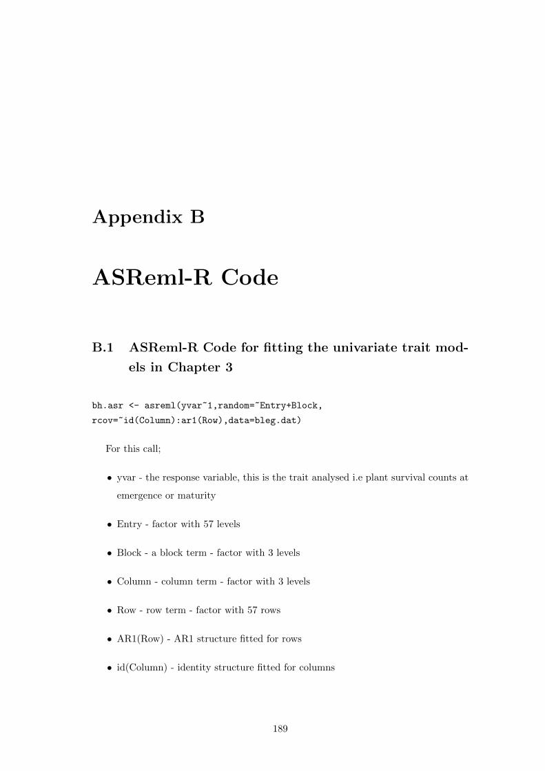
Appendix B
ASReml-R Code
B.1 ASReml-R Code for fitting the univariate trait mod-
els in Chapter 3
bh.asr <- asreml(yvar~1,random=~Entry+Block,
rcov=~id(Column):ar1(Row),data=bleg.dat)
For this call;
• yvar - the response variable, this is the trait analysed i.e plant survival counts at
emergence or maturity
• Entry - factor with 57 levels
• Block - a block term - factor with 3 levels
• Column - column term - factor with 3 levels
• Row - row term - factor with 57 rows
• AR1(Row) - AR1 structure fitted for rows
• id(Column) - identity structure fitted for columns
189

B. ASREML-R CODE
B.2 ASReml-R Code for fitting the bivariate trait models
in Chapter 3
bh.asr <-asreml(yvar~Sample,random=~corh(Sample):Entry+diag(Sample):Block
+at(Sample,’eme’):Row,
rcov=~corh(Sample):id(Column):ar1(Row),data= bleg.dat)
For this call;
• Sample - factor with two levels corresponding to the traits emergence and maturity
• Entry - factor with 57 levels
• Block - a block term - factor with 3 levels
• Column - column term - factor with 3 levels
• Row - row term factor with 57 rows
• AR1(Row) - AR1 structure fitted for rows
• id(Column) - identity structure fitted for columns
190

Bibliography
ABARES (2011). Agricultural commodity statistics 2011. Canberra, Australia. 7
ABARES (2012). Agricultural commodity statistics 2012. Canberra, Australia. 1
ABS (2008). Agricultural commodities: Small area data, Australia, 2005-06 (Reissue). Australia. 2
Allard, R. W. (1999). Principles of plant breeding. John Wiley & Sons, New York, 2nd edition. 2
Ansan Melayah, D., Rouxel, T., Bertrandy, J., Letarnec, B., Mendes Pereira, E., and Balesdent, M. H. (1997).
Field efficiency of Brassica napus specific resistance correlates with Leptosphaeria maculans population
structure. European Journal of Plant Pathology, 103(9):835–841. 10
Argillier, O., Hebert, Y., and Barriere, Y. (1994). Statistical analysis and interpretation of line x environment
interaction for biomass yield in maize. Agronomie, 14(10):661–672. 58, 106
Atkin, F., Dieters, M., and Stringer, J. (2009). Impact of depth of pedigree and inclusion of historical data on
the estimation of additive variance and breeding values in a sugarcane breeding program. Theoretical and
Applied Genetics, 119(3):555–565. 4, 142
Atkinson, A. (1985). Plots, transformations, and regression: an introduction to graphical methods of diagnostic
regression analysis. Clarendon Press, Oxford. 87
Atlin, G., Enerson, P., McGirr, L., and Hunter, R. (1983). Gibberella ear rot development and zearalenone and
vomitoxin production as affected by maize genotype and Gibberella zeae strain. Canadian Journal of Plant
Science, 63(4):847–853. 48, 49
Balesdent, M. H., Attard, A., Ansan-Melayah, D., Delourme, R., Renard, M., and Rouxel, T. (2001). Genetic
control and host range of avirulence toward Brassica napus cultivars Quinta and Jet Neuf in Leptosphaeria
maculans. Phytopathology, 91(1):70–76. 10, 136
Balestre, M., Torga, P., Von Pinho, R., and dos Santos, J. (2012). Applications of multi-trait selection in
common bean using real and simulated experiments. Euphytica, 189(2):225–238. 45
Ballinger, D. J. and Salisbury, P. A. (1996). Seedling and adult plant evaluation of race variability in Lep-
tosphaeria maculans on Brassica species in Australia. Australian Journal of Experimental Agriculture,
36(4):485–488. 10, 165
Balzarini, M. (2002). Applications of mixed models in plant breeding. In Kang, M., editor, Quantitative genetics,
genomics and plant breeding, pages 353–363. CAB International, Wallingford, Oxford. 62
Barbetti, M. and Khangura, R. (1999). Managing blackleg in the disease-prone environment of Western Aus-
tralia. In N, W., editor, 10th International Rapeseed Congress, Canberra, Australia. 8
191

BIBLIOGRAPHY
Basford, K. E. and Cooper, M. (1998). Genotype x environment interactions and some considerations of their
implications for wheat breeding in Australia. Australian Journal of Agricultural Research, 49(2):153–174.
58, 101, 167
Bauer, A., Hoti, F., Reetz, T., Schuh, W., Leon, J., and Sillanpaa, M. (2009). Bayesian prediction of breeding
values by accounting for genotype-by-environment interaction in self-pollinating crops. Genetics Research,
91(3):193–207. 3, 57
Bauer, A., Reetz, T., and Leon, J. (2006). Estimation of breeding values of inbred lines using best linear unbiased
prediction (BLUP) and genetic similarities. Crop Science, 46(6):2685. 67, 68, 69
Beeck, C., Cowling, W., Smith, A., and Cullis, B. (2010). Analysis of yield and oil from a series of canola breeding
trials. Part 1. Fitting factor analytic mixed models with pedigree information. Genome, 53(11):992–1001. 4,
57, 58, 61, 62, 64, 65, 66, 68, 71, 83, 85, 132, 133, 134, 137, 141, 142, 166, 168
Bernardo, R. (1993). Estimation of coefficient of coancestry using molecular markers in maize. Theoretical and
Applied Genetics, 85(8):1055–1062. 64, 65, 67, 68, 69
Bernardo, R. (1994). Prediction of maize single-cross performance using RFLPs and information from related
hybrids. Crop Science, 34(1):20–25. 58, 62, 63, 64, 65, 66, 67, 68
Bernardo, R. (1995). Genetic models for predicting maize single-cross performance in unbalanced yield trial
data. Crop Science, 35(1):141–147. 58, 63, 64, 65, 67, 70
Bernardo, R. (1996a). Best linear unbiased prediction of maize single-cross performance. Crop Science, 36(1):50–
56. 63, 64, 65
Bernardo, R. (1996b). Testcross additive and dominance effects in best linear unbiased prediction of maize
single-cross performance. Theoretical and Applied Genetics, 93(7):1098–1102. 63, 64, 65
Bernardo, R. (2002). Breeding for quantitative traits in plants. Stemma Press Woodburn, Minnesota, 2nd
edition. 63, 106, 134
Bernardo, R., Murigneux, A., and Karaman, Z. (1996). Marker-based estimates of identity by descent and
alikeness in state among maize inbreds. Theoretical and Applied Genetics, 93(1):262–267. 64, 67, 68
Bernardo, R., Romero-Severson, J., Ziegle, J., Hauser, J., Joe, L., Hookstra, G., and Doerge, R. (2000). Parental
contribution and coefficient of coancestry among maize inbreds: pedigree, RFLP, and SSR data. Theoretical
and Applied Genetics, 100(3):552–556. 68
Blanco, A., Mangini, G., Giancaspro, A., Giove, S., Colasuonno, P., Simeone, R., Signorile, A., De Vita, P.,
Mastrangelo, A., Cattivelli, L., et al. (2012). Relationships between grain protein content and grain yield
components through quantitative trait locus analyses in a recombinant inbred line population derived from
two elite durum wheat cultivars. Molecular Breeding, 30(1):79–92. 54, 56
Brandle, J. and McVetty, P. (1989). Effects of inbreeding and estimates of additive genetic variance within seven
summer oilseed rape cultivars. Genome, 32(1):115–119. 135
Burgueno, J., Crossa, J., Cornelius, P., Trethowan, R., McLaren, G., and Krishnamachari, A. (2007). Modeling
additive x environment and additive x additive x environment using genetic covariances of relatives of wheat
genotypes. Crop Science, 47(1):311–320. 57, 60, 64, 65, 66, 70, 83, 166
Busbice, T. (1969). Inbreeding in synthetic varieties. Crop Science, 9(5):601–604. 78
Butler, D. (2012). Pedicure: pedigree fun, R package version 0.1. Queensland DPI, Brisbane, Australia. 79,
106, 158
192

BIBLIOGRAPHY
Butler, D., Cullis, B., Gilmour, A., and Gogel, B. (2009). Mixed models for S language environments, ASReml-R
reference manual. Queensland DPI, Brisbane, Australia. 21, 77, 89
Cadalen, T., Sourdille, P., Charmet, G., Tixier, M., Gay, G., Boeuf, C., Bernard, S., Leroy, P., and Bernard, M.
(1998). Molecular markers linked to genes affecting plant height in wheat using a doubled-haploid population.
Theoretical and Applied Genetics, 96(6):933–940. 52
Can, N., Nakamura, S., and Yoshida, T. (1997). Combining ability and genotype x environmental interaction
in early maturing grain sorghum for summer seeding. Japanese Journal of Crop Science, 66(4):698–705. 60
Chapman, S., Cooper, M., Podlich, D., and Hammer, G. (2003). Evaluating plant breeding strategies by
simulating gene action and dryland environment effects. Agronomy Journal, 95(1):99–113. 2
Cochran, W. (1957). Analysis of covariance: its Nature and Uses. Biometrics, 13(3):261–281. 41, 46, 51, 55
Comstock, R. E. et al. (1996). Quantitative genetics with special reference to plant and animal breeding. Iowa
State University Press, Ames, Iowa, 1st edition. 1, 3, 164
Coombes, N. (2009). Digger, a spatial design program. Technical report, NSW Department of Primary Industries.
74
Cooper, M. and DeLacy, I. H. (1994). Relationships among analytical methods used to study genotypic variation
and genotype-by-environment interaction in plant breeding multi-environment experiments. Theoretical and
Applied Genetics, 88(5):561–572. 58, 106, 134
Cooper, M., DeLacy, I. H., and Basford, K. E. (1996). Relationships among analytical methods used to study
genotypic variation and genotype-by-environment interaction in plant breeding multi-environment experi-
ments. In Cooper, M. and Hammer, G., editors, Plant adaptation and crop improvement, pages 193–224.
CAB International, Wallingford, Oxford. xvii, 58, 59
Cooper, M., Podlich, D., and Smith, O. (2005). Gene-to-phenotype models and complex trait genetics. Australian
Journal of Agricultural Research, 56(9):895–918. 3, 171
Cowling, W. A. (2007). Genetic diversity in Australian canola and implications for crop breeding for changing
future environments. Field Crops Research, 104(1-3):103–111. 75
Crossa, J., Burgueno, J., Cornelius, P., McLaren, G., Trethowan, R., and Krishnamachari, A. (2006). Modeling
genotype x environment interaction using additive genetic covariances of relatives for predicting breeding
values of wheat genotypes. Crop Science, 46(4):1722–1733. 4, 57, 61, 65, 66, 83, 103, 123, 133, 142, 166, 168
Cullis, B., Gogel, B., Verbyla, A., and Thompson, R. (1998). Spatial analysis of multi-environment early
generation variety trials. Biometrics, 54(1):1–18. 11, 56, 82, 102
Cullis, B., Smith, A., Beeck, C., and Cowling, W. (2010). Analysis of yield and oil from a series of canola breeding
trials. Part ii. Exploring variety by environment interaction using factor analysis. Genome, 53(11):1002–1016.
4, 57, 58, 60, 61, 62, 64, 68, 71, 112, 123, 127, 132, 134, 137, 141, 142, 166, 168
Cullis, B., Smith, A., and Coombes, N. (2006). On the design of early generation variety trials with correlated
data. Journal of Agricultural, Biological, and Environmental Statistics, 11(4):381–393. 11, 74, 82, 83, 101,
167
de la Vega, A. and Chapman, S. (2006). Multivariate analyses to display interactions between environment and
general or specific combining ability in hybrid crops. Crop Science, 46(2):957–967. 105
de Resende, M., Thompson, R., and Welham, S. (2006). Multivariate spatial statistical analysis of longitudinal
data in perennial crops. Revista de Matematica e Estatıstica, 24(1):147–169. 12
193

BIBLIOGRAPHY
Delourme, R., Brun, H., Ermel, M., Lucas, M. O., Vallee, P., Domin, C., Walton, G., Hua, L., Sivasithamparam,
K., and Barbetti, M. J. (2008). Expression of resistance to Leptosphaeria maculans in Brassica napus double
haploid lines in France and Australia is influenced by location. Annals of Applied Biology, 153(2):259–269.
10, 136
Du, F. and Hoeschele, I. (2000). Estimation of additive, dominance and epistatic variance components using
finite locus models implemented with a single-site Gibbs and a descent graph sampler. Genetical Research,
76(02):187–198. 60
Dutkowski, G., Costa e Silva, J., Gilmour, A., Wellendorf, H., and Aguiar, A. (2006). Spatial analysis enhances
modelling of a wide variety of traits in forest genetic trials. Canadian Journal of Forest Research, 36(7):1851–
1870. 11, 12, 56, 82
Eisenhart, C. (1947). The assumptions underlying the analysis of variance. Biometrics, 3(1):1–21. 61
Elashoff, J. (1969). Analysis of covariance: A delicate instrument. American Educational Research Journal,
6(3):383–401. 46
Ellis, R., Hong, T., and Jackson, M. (1993). Seed production environment, time of harvest, and the potential
longevity of seeds of three cultivars of rice (Oryza sativa L.). Annals of Botany, 72(6):583–590. 11, 41
Ellis, R. and Roberts, E. (1980). Improved equations for the prediction of seed longevity. Annals of Botany,
45(1):13. 11, 41
Emebiri, L., Moody, D., Panozzo, J., and Read, B. (2004). Mapping of QTL for malting quality attributes in
barley based on a cross of parents with low grain protein concentration. Field Crops Research, 87(2):195–205.
54, 56
Emrich, K., Wilde, F., Miedaner, T., and Piepho, H. (2008). REML approach for adjusting the Fusarium head
blight rating to a phenological date in inoculated selection experiments of wheat. Theoretical and Applied
Genetics, 117(1):65–73. 47, 48, 52, 55
Falconer, D. (1981). Introduction to quantitative genetics. Longman, London, U.K., 2nd edition. 65, 105, 166
Finch Savage, W. E. (1986). A study of the relationship between seedling characters and rate of germination
within a seed lot. Annals of Applied Biology, 108(2):441–444. 11, 41, 47, 50
Fitt, B. D. L., Brun, H., Barbetti, M. J., and Rimmer, S. R. (2006). World-wide importance of phoma stem
canker (Leptosphaeria maculans and L. biglobosa) on oilseed rape (Brassica napus). European Journal of
Plant Pathology, 114(1):3–15. 6, 8, 10, 136
Forcella, F., Benech Arnold, R., Sanchez, R., and Ghersa, C. (2000). Modeling seedling emergence. Field Crops
Research, 67(2):123–139. 11, 41, 49
Frensham, A., Cullis, B., and Verbyla, A. (1997). Genotype by environment variance heterogeneity in a two-stage
analysis. Biometrics, 53(4):1373–1383. 57
Fukai, S. and Cooper, M. (1995). Development of drought-resistant cultivars using physiomorphological traits
in rice. Field Crops Research, 40(2):67–86. 106, 168
Gilmour, A., Cullis, B., and Verbyla, A. (1997). Accounting for natural and extraneous variation in the analysis
of field experiments. Journal of Agricultural, Biological, and Environmental Statistics, 2(3):269–293. 9, 11,
18, 20, 39, 65, 82, 87, 102
Gilmour, A. R., Thompson, R., and Cullis, B. R. (1995). Average information REML: An efficient algorithm
for variance parameter estimation in linear mixed models. Biometrics, 51(4):1440–1450. 142, 153, 154
194
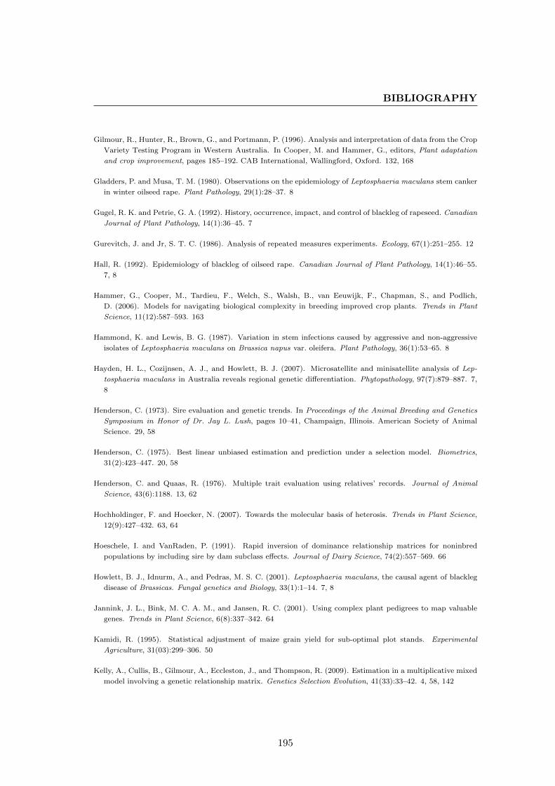
BIBLIOGRAPHY
Gilmour, R., Hunter, R., Brown, G., and Portmann, P. (1996). Analysis and interpretation of data from the Crop
Variety Testing Program in Western Australia. In Cooper, M. and Hammer, G., editors, Plant adaptation
and crop improvement, pages 185–192. CAB International, Wallingford, Oxford. 132, 168
Gladders, P. and Musa, T. M. (1980). Observations on the epidemiology of Leptosphaeria maculans stem canker
in winter oilseed rape. Plant Pathology, 29(1):28–37. 8
Gugel, R. K. and Petrie, G. A. (1992). History, occurrence, impact, and control of blackleg of rapeseed. Canadian
Journal of Plant Pathology, 14(1):36–45. 7
Gurevitch, J. and Jr, S. T. C. (1986). Analysis of repeated measures experiments. Ecology, 67(1):251–255. 12
Hall, R. (1992). Epidemiology of blackleg of oilseed rape. Canadian Journal of Plant Pathology, 14(1):46–55.
7, 8
Hammer, G., Cooper, M., Tardieu, F., Welch, S., Walsh, B., van Eeuwijk, F., Chapman, S., and Podlich,
D. (2006). Models for navigating biological complexity in breeding improved crop plants. Trends in Plant
Science, 11(12):587–593. 163
Hammond, K. and Lewis, B. G. (1987). Variation in stem infections caused by aggressive and non-aggressive
isolates of Leptosphaeria maculans on Brassica napus var. oleifera. Plant Pathology, 36(1):53–65. 8
Hayden, H. L., Cozijnsen, A. J., and Howlett, B. J. (2007). Microsatellite and minisatellite analysis of Lep-
tosphaeria maculans in Australia reveals regional genetic differentiation. Phytopathology, 97(7):879–887. 7,
8
Henderson, C. (1973). Sire evaluation and genetic trends. In Proceedings of the Animal Breeding and Genetics
Symposium in Honor of Dr. Jay L. Lush, pages 10–41, Champaign, Illinois. American Society of Animal
Science. 29, 58
Henderson, C. (1975). Best linear unbiased estimation and prediction under a selection model. Biometrics,
31(2):423–447. 20, 58
Henderson, C. and Quaas, R. (1976). Multiple trait evaluation using relatives’ records. Journal of Animal
Science, 43(6):1188. 13, 62
Hochholdinger, F. and Hoecker, N. (2007). Towards the molecular basis of heterosis. Trends in Plant Science,
12(9):427–432. 63, 64
Hoeschele, I. and VanRaden, P. (1991). Rapid inversion of dominance relationship matrices for noninbred
populations by including sire by dam subclass effects. Journal of Dairy Science, 74(2):557–569. 66
Howlett, B. J., Idnurm, A., and Pedras, M. S. C. (2001). Leptosphaeria maculans, the causal agent of blackleg
disease of Brassicas. Fungal genetics and Biology, 33(1):1–14. 7, 8
Jannink, J. L., Bink, M. C. A. M., and Jansen, R. C. (2001). Using complex plant pedigrees to map valuable
genes. Trends in Plant Science, 6(8):337–342. 64
Kamidi, R. (1995). Statistical adjustment of maize grain yield for sub-optimal plot stands. Experimental
Agriculture, 31(03):299–306. 50
Kelly, A., Cullis, B., Gilmour, A., Eccleston, J., and Thompson, R. (2009). Estimation in a multiplicative mixed
model involving a genetic relationship matrix. Genetics Selection Evolution, 41(33):33–42. 4, 58, 142
195

BIBLIOGRAPHY
Kelly, A. M., Smith, A. B., Eccleston, J. A., and Cullis, B. R. (2007). The accuracy of varietal selection using
factor analytic models for multi-environment plant breeding trials. Crop Science, 47(3):1063–1070. 57, 61,
83, 132
Kerr, R. (1998). Asymptotic rates of response from forest tree breeding strategies using best linear unbiased
prediction. Theoretical and Applied Genetics, 96(3):484–493. 13
Khangura, R. K. and Barbetti, M. J. (2001). Prevalence of blackleg (Leptosphaeria maculans) on canola
(Brassica napus) in Western Australia. Australian Journal of Experimental Agriculture, 41(1):71–80. 7, 10
Kidwell, J. (1963). Genotype x environment interaction with isogenic lines of Drosophila Melanogaster. Genetics,
48(12):1593–1604. 60, 69
Kirkegaard, J., Peoples, M., Angus, J., and Unkovich, M. (2011). Diversity and evolution of rainfed farming
systems in Southern Australia. In Tow, P., Cooper, I., Partridge, I., and Birch, C., editors, Rainfed Farming
Systems, pages 715–754. Springer, Netherlands. 2, 137
Kirkegaard, J. and Sarwar, M. (1999). Glucosinolate profiles of Australian canola (Brassica napus annua L.)
and Indian mustard (Brassica juncea L.) cultivars: implications for biofumigation. Australian Journal of
Agricultural Research, 50(3):315–324. 7
Kirkegaard, J. A., Robertson, M. J., Hamblin, P., and Sprague, S. J. (2006). Effect of blackleg and sclerotinia
stem rot on canola yield in the high rainfall zone of southern New South Wales, Australia. Australian Journal
of Agricultural Research, 57(2):201–212. 8
Klahr, A., Zimmermann, G., Wenzel, G., and Mohler, V. (2007). Effects of environment, disease progress, plant
height and heading date on the detection of QTLs for resistance to Fusarium head blight in an european
winter wheat cross. Euphytica, 154(1):17–28. 52, 56
Korol, A., Ronin, Y., and Kirzhner, V. (1995). Interval mapping of quantitative trait loci employing correlated
trait complexes. Genetics, 140(3):1137–1147. 56
Kuchel, H., Langridge, P., Mosionek, L., Williams, K., and Jefferies, S. (2006). The genetic control of milling
yield, dough rheology and baking quality of wheat. Theoretical and Applied Genetics, 112(8):1487–1495. 54,
56
Leask, W. and Daynard, T. (1973). Dry matter yield, in vitro digestibility, percent protein, and moisture of
corn stover following grain maturity. Canadian Journal of Plant Science, 53(3):515–522. 51
Leflon, M., Brun, H., Eber, F., Delourme, R., Lucas, M. O., Vallee, P., Ermel, M., Balesdent, M. H., and Chevre,
A. M. (2007). Detection, introgression and localization of genes conferring specific resistance to Leptosphaeria
maculans from Brassica rapa into B. napus. Theoretical and Applied Genetics, 115(7):897–906. 10
Li, C. X., Wratten, N., Salisbury, P. A., Burton, W. A., Potter, T. D., Walton, G., Li, H., Sivasithamparam,
K., Banga, S. S., and Banga, S. (2008). Response of Brassica napus and B. juncea germplasm from Aus-
tralia, China and India to Australian populations of Leptosphaeria maculans. Australasian Plant Pathology,
37(2):162–170. 6, 9
Li, H., Sivasithamparam, K., and Barbetti, M. J. (2007). Soilborne ascospores and pycnidiospores of Lep-
tosphaeria maculans can contribute significantly to blackleg disease epidemiology in oilseed rape (Brassica
napus) in Western Australia. Australasian Plant Pathology, 36(5):439–444. 10, 40, 47
Li, Z., Pinson, S., Stansel, J., and Park, W. (1995). Identification of quantitative trait loci (QTLs) for heading
date and plant height in cultivated rice (Oryza sativa L.). Theoretical and Applied Genetics, 91(2):374–381.
53
196

BIBLIOGRAPHY
Li, Z., Yu, S., Lafitte, H., Huang, N., Courtois, B., Hittalmani, S., Vijayakumar, C., Liu, G., Wang, G., and
Shashidhar, H. (2003). QTL × environment interactions in rice. I. Heading date and plant height. Theoretical
and Applied Genetics, 108(1):141–153. 53
Light, K., Gororo, N., and Salisbury, P. (2011). Usefulness of winter canola (Brassica napus) race-specific
resistance genes against blackleg (causal agent Leptosphaeria maculans) in southern Australian growing
conditions. Crop and Pasture Science, 62(2):162–168. 165
Lin, C., McAllister, A., and Lee, A. (1985). Multitrait estimation of relationships of first-lactation yields to
body weight changes in Holstein heifers. Journal of Dairy Science, 68(11):2954–2963. 3, 13, 56
Lippman, Z. and Zamir, D. (2007). Heterosis: revisiting the magic. Trends in Genetics, 23(2):60–66. 64
Littell, R., Henry, P., and Ammerman, C. (1998). Statistical analysis of repeated measures data using SAS
procedures. Journal of Animal Science, 76(4):1216–1231. 12
Littley, E. and Rahe, J. (1987). Effect of host plant density on white rot of onion caused by Sclerotium cepivorum.
Canadian Journal of Plant Pathology, 9(2):146–151. 49, 50
Liu, X. and Wu, J. (1998). SSR heterogenic patterns of parents for marking and predicting heterosis in rice
breeding. Molecular Breeding, 4(3):263–268. 60, 69
Lynch, M. and Walsh, B. (1998). Genetics and analysis of quantitative traits. Sinauer Associates Sunderland,
MA. 2, 60, 63, 64
Maenhout, S., De Baets, B., and Haesaert, G. (2009). Marker-based estimation of the coefficient of coancestry
in hybrid breeding programmes. Theoretical and Applied Genetics, 118(6):1181–1192. 64, 67, 69, 171
Maenhout, S., De Baets, B., and Haesaert, G. (2010). Prediction of maize single-cross hybrid performance:
support vector machine regression versus best linear prediction. Theoretical and Applied Genetics, 120(2):415–
427. 63, 68, 69
Malosetti, M., van Eeuwijk, F., Boer, M., Casas, A., ElIa, M., Moralejo, M., Bhat, P., Ramsay, L., and Molina-
Cano, J. (2011). Gene and QTL detection in a three-way barley cross under selection by a mixed model with
kinship information using SNPs. Theoretical and Applied Genetics, 122:1605–1616. 61
Marcroft, S. (2009). Site blackleg quality assuarnce report 2002 - 2009. Technical report, Marcroft Grains
Pathology. 16, 40
Marcroft, S., Van de Wouw, A., Salisbury, P., Potter, T., and Howlett, B. (2012). Effect of rotation of canola
(Brassica napus) cultivars with different complements of blackleg resistance genes on disease severity. Plant
Pathology, 61(5):934–944. 6, 9
Marcroft, S. J., Purwantara, A., Salisbury, P. A., Potter, T. D., Wratten, N., Khangura, R., Barbetti, M. J.,
and Howlett, B. J. (2002). Reaction of a range of Brassica species under Australian conditions to the
fungus, Leptosphaeria maculans, the causal agent of blackleg. Australian Journal of Experimental Agriculture,
42(5):587–594. 8, 9
Mather, K. and Jinks, J. (1982). Biometrical genetics: the study of continuous variation. Chapman & Hall,
London, U.K. 61
Mathews, K., Chapman, S., Trethowan, R., Pfeiffer, W., Van Ginkel, M., Crossa, J., Payne, T., DeLacy, I., Fox,
P., and Cooper, M. (2007). Global adaptation patterns of Australian and CIMMYT spring bread wheat.
Theoretical and Applied Genetics, 115(6):819–835. 142
197

BIBLIOGRAPHY
McGee, D. C. and Emmett, R. W. (1977). Blackleg (Leptosphaeria maculans (Desm.) Ces. et de Not.) of
rapeseed in Victoria: crop losses and factors which affect disease severity. Australian Journal of Agricultural
Research, 28(1):47–51. 8
Melchinger, A., Lee, M., Lamkey, K., Hallauer, A., and Woodman, W. (1990). Genetic diversity for restriction
fragment length polymorphisms and heterosis for two diallel sets of maize inbreds. Theoretical and Applied
Genetics, 80(4):488–496. 67
Meuwissen, T. and Luo, Z. (1992). Computing inbreeding coefficients in large populations. Genetics Selection
Evolution, 24(4):1–9. 79, 89
Meyer, K. (1989). Restricted maximum likelihood to estimate variance components for animal models with
several random effects using a derivative-free algorithm. Genetics Selection Evolution, 21:317–340. 154
Misztal, I. (1997). Estimation of variance components with large-scale dominance models. Journal of Dairy
Science, 80(5):965–974. 60
Mrode, R. A. and Thompson, R. (2005). Linear models for the prediction of animal breeding values. CABI
Publishing, Wallingford, U.K., 2nd edition. 13, 29, 56, 171
Norton, R., Kirkegaard, J., Angus, J., and Potter, T. (1999). Canola in rotations. In Proceedings of the 10th
International Rapeseed Congress 1999, pages 23–28, Canberra, Australia. 1
Oakey, H., Verbyla, A., Cullis, B., Wei, X., and Pitchford, W. (2007). Joint modeling of additive and non-additive
(genetic line) effects in multi-environment trials. Theoretical and Applied Genetics, 114(8):1319–1332. 3, 4,
57, 58, 61, 62, 65, 66, 67, 71, 77, 83, 85, 106, 110, 112, 123, 132, 133, 141, 168
Oakey, H., Verbyla, A., Pitchford, W., Cullis, B., and Kuchel, H. (2006). Joint modeling of additive and non-
additive genetic line effects in single field trials. Theoretical and Applied Genetics, 113(5):809–819. 3, 61, 62,
64, 65, 66, 71, 83, 85, 86, 102, 132, 133, 141, 168
Ovaskainen, O., Cano, J., and Merila, J. (2008). A Bayesian framework for comparative quantitative genetics.
Proceedings of the Royal Society B: Biological Sciences, 275(1635):669–678. 60
Parlevliet, J. (1979). Components of resistance that reduce the rate of epidemic development. Annual Review
of Phytopathology, 17(1):203–222. 6
Patterson, H. and Thompson, R. (1971). Recovery of inter-block information when block sizes are unequal.
Biometrika, 58(3):545–554. 20, 142
Piepho, H., Mohring, J., Melchinger, A., and Buchse, A. (2008). BLUP for phenotypic selection in plant breeding
and variety testing. Euphytica, 161(1):209–228. 3, 4, 13, 45, 57, 61, 65, 67, 69, 164
Piepho, H. P. and Mohring, J. (2006). Selection in cultivar trials-Is it ignorable? Crop Science, 46(1):192–201.
12
Pilet, M., Delourme, R., Foisset, N., and Renard, M. (1998). Identification of loci contributing to quantitative
field resistance to blackleg disease, causal agent Leptosphaeria maculans (Desm.) Ces. et de Not., in winter
rapeseed (Brassica napus L.). Theoretical and Applied Genetics, 96(1):23–30. 6
Pixley, K. and Bjarnason, M. (2002). Stability of grain yield, endosperm modification, and protein quality of
hybrid and open-pollinated quality protein maize (QPM) cultivars. Crop Science, 42(6):1882–1890. 51
Pollak, E., Van der Werf, J., and Quaas, R. (1984). Selection bias and multiple trait evaluation. Journal of
Dairy Science, 67(7):1590–1595. 13
198

BIBLIOGRAPHY
Pordesimo, L., Edens, W., and Sokhansanj, S. (2004). Distribution of aboveground biomass in corn stover.
Biomass and Bioenergy, 26(4):337–343. 51
Punithalingam, E. and Holliday, P. (1972). Leptosphaeria maculans. In IMI Descriptions of Fungi and Bacteria,
page 331. Commonwealth Mycological Institute. 6
R Development Core Team (2012). R: A language and environment for statistical computing, Vienna, Austria.
http://www.R-project.org/. 89, 106, 112, 158
Raymer, P. L. (2002). Canola: An emerging oilseed crop. In Janick, J. and A, W., editors, Trends in new crops
and new uses, pages 122–126. ASHS Press: Alexandria, VA. 1
Rempel, C. and Hall, R. (1996). Comparison of disease measures for assessing resistance in canola (Brassica
napus) to blackleg (Leptosphaeria maculans). Canadian Journal of Botany, 74(12):1930–1936. 6, 9, 10, 12,
165
Riaz, A., Li, G., Quresh, Z., Swati, M. S., and Quiros, C. F. (2001). Genetic diversity of oilseed Brassica napus
inbred lines based on sequence-related amplified polymorphism and its relation to hybrid performance. Plant
Breeding, 120(5):411–415. 58
Rimmer, S. R. and Van den Berg, C. G. J. (1992). Resistance of oilseed Brassica spp. to blackleg caused by
Leptosphaeria maculans. Journal of Plant Pathology, 14(1):56–66. 8
Roy, N. N. (1984). Interspecific transfer of Brassica juncea - type high blackleg resistance to Brassica napus.
Euphytica, 33(2):295–303. 10, 165
Salisbury, P. and Wratten, N. (1999). Brassica napus breeding. In Salisbury, P., Potter, T., McDonald, G., and
Green, A., editors, Canola in Australia: the First 30 Years, pages 29–35. Organising Committee of the 10th
International Rapeseed Congress. 2, 75
Schrag, T., Melchinger, A., Srensen, A., and Frisch, M. (2006). Prediction of single-cross hybrid performance
for grain yield and grain dry matter content in maize using AFLP markers associated with QTL. Theoretical
and Applied Genetics, 113(6):1037–1047. 63
Schrag, T., Mohring, J., Maurer, H., Dhillon, B., Melchinger, A., Piepho, H., Sorensen, A., and Frisch, M.
(2009). Molecular marker-based prediction of hybrid performance in maize using unbalanced data from
multiple experiments with factorial crosses. Theoretical and Applied Genetics, 118(4):741–751. 63
Schrag, T., Mohring, J., Melchinger, A., Kusterer, B., Dhillon, B., Piepho, H., and Frisch, M. (2010). Prediction
of hybrid performance in maize using molecular markers and joint analyses of hybrids and parental inbreds.
Theoretical and Applied Genetics, 120(2):451–461. 63
Si, P., Mailer, R., Galwey, N., and Turner, D. (2003). Influence of genotype and environment on oil and protein
concentrations of canola (Brassica napus l.) grown across southern Australia. Crop and Pasture Science,
54(4):397–407. 135
Sivasithamparam, K., Barbetti, M. J., and Li, H. (2005). Recurring challenges from a necrotrophic fungal
plant pathogen: a case study with Leptosphaeria maculans (causal agent of blackleg disease in Brassicas) in
Western Australia. Annals of Botany, 96(3):363–377. 10
Smith, A., Cullis, B., Luckett, D., Hollamby, G., and Thompson, R. (2002a). Exploring variety-environment
data using random effects AMMI models with adjustments for spatial field trend: Part 2: Applications. In
Kang, M., editor, Quantitative Genetics, Geonomics and Plant Breeding, chapter 22, pages 337–351. CABI
Publishing, Wallingford, U.K. 56, 66, 81, 82
199

BIBLIOGRAPHY
Smith, A., Cullis, B., and Thompson, R. (2001a). The analysis of crop variety evaluation data in Australia.
Australian & New Zealand Journal of Statistics, 43(2):129–145. 61, 62, 82, 102
Smith, A., Cullis, B., and Thompson, R. (2001b). Analyzing Variety by Environment Data Using Mulitplicative
Mixed Models and Adjustments for Spatial Field Trend. Biometrics, 57(4):1138–1147. 9, 56, 61, 82, 102,
106, 110, 112, 132, 142, 143, 144, 157
Smith, A., Cullis, B., and Thompson, R. (2002b). Exploring variety-environment data using random effects
AMMI models with adjustments for spatial field trend: Part1: Theory. In Kang, M., editor, Quantitative
Genetics, Geonomics and Plant Breeding, chapter 21, pages 323–335. CABI Publishing, Wallingford, U.K.
4, 9, 82, 86
Smith, A., Cullis, B., and Thompson, R. (2005). The analysis of crop cultivar breeding and evaluation trials:
an overview of current mixed model approaches. The Journal of Agricultural Science, 143(06):449–462. 61,
132
Smith, A., Lim, P., and Cullis, B. (2006). The design and analysis of multi-phase plant breeding experiments.
The Journal of Agricultural Science, 144(05):393–409. 82
Smith, H. (1957). Interpretation of adjusted treatment means and regressions in analysis of covariance. Bio-
metrics, 13(3):282–308. 46, 47, 50, 55
Smith, J., Duvick, D., Smith, O., Cooper, M., and Feng, L. (2004). Changes in pedigree backgrounds of Pioneer
brand maize hybrids widely grown from 1930 to 1999. Crop Science, 44(6):1935–1946. 65
Sosnowski, M. R., Scott, E. S., and Ramsey, M. D. (2006). Survival of Leptosphaeria maculans in soil on residues
of Brassica napus in South Australia. Plant Pathology, 55(2):200–206. 10, 40, 47
Stefanova, K. and Buirchell, B. (2010). Multiplicative mixed models for genetic gain assessment in lupin breeding.
Crop Science, 50(3):880–891. 132
Stefanova, K., Smith, A., and Cullis, B. (2009). Enhanced diagnostics for the spatial analysis of field trials.
Journal of Agricultural, Biological, and Environmental Statistics, 14(4):392–410. 4, 81, 82, 83, 87, 88, 102
Stelmakh, A. (1992). Genetic effects of vrn genes on heading date and agronomic traits in bread wheat. Euphytica,
65(1):53–60. 48
Stringer, J., Cullis, B., and Thompson, R. (2011). Joint modeling of spatial variability and within-row inter-
plot competition to increase the efficiency of plant improvement. Journal of Agricultural, Biological, and
Environmental Statistics, 16(2):269–281. 81
Tester, M. and Langridge, P. (2010). Breeding technologies to increase crop production in a changing world.
Science, 327(5967):818–822. 1
Thompson, R. (2009). Latent mixed models. In Proceedings of the eighteenth Association for the Advancement of
Animal Breeding and Genetics, volume Statistical methods 1, pages 398–405, Adelaide, Australia. Association
for the Advancement of Animal Breeding and Genetics. 153, 154, 157
Thompson, R., Cullis, B., Smith, A., and Gilmour, A. (2003). A sparse implementation of the average information
algorithm for factor analytic and reduced rank variance models. Australian & New Zealand Journal of
Statistics, 45(4):445–459. 143, 147, 150, 154, 157
Thompson, R. and Meyer, K. (1986). A review of theoretical aspects in the estimation of breeding values for
multi-trait selection. Livestock Production Science, 15(4):299–313. 13, 29, 56
200
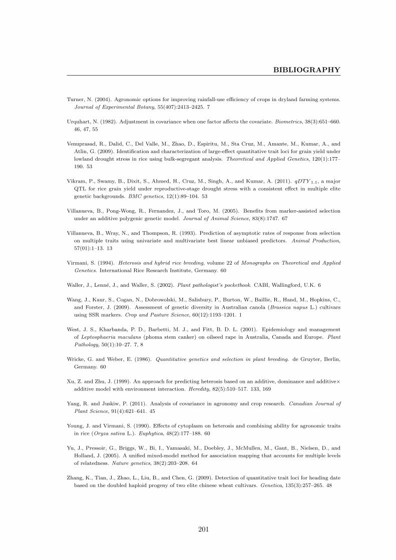
BIBLIOGRAPHY
Turner, N. (2004). Agronomic options for improving rainfall-use efficiency of crops in dryland farming systems.
Journal of Experimental Botany, 55(407):2413–2425. 7
Urquhart, N. (1982). Adjustment in covariance when one factor affects the covariate. Biometrics, 38(3):651–660.
46, 47, 55
Venuprasad, R., Dalid, C., Del Valle, M., Zhao, D., Espiritu, M., Sta Cruz, M., Amante, M., Kumar, A., and
Atlin, G. (2009). Identification and characterization of large-effect quantitative trait loci for grain yield under
lowland drought stress in rice using bulk-segregant analysis. Theoretical and Applied Genetics, 120(1):177–
190. 53
Vikram, P., Swamy, B., Dixit, S., Ahmed, H., Cruz, M., Singh, A., and Kumar, A. (2011). qDTY 1.1, a major
QTL for rice grain yield under reproductive-stage drought stress with a consistent effect in multiple elite
genetic backgrounds. BMC genetics, 12(1):89–104. 53
Villanueva, B., Pong-Wong, R., Fernandez, J., and Toro, M. (2005). Benefits from marker-assisted selection
under an additive polygenic genetic model. Journal of Animal Science, 83(8):1747. 67
Villanueva, B., Wray, N., and Thompson, R. (1993). Prediction of asymptotic rates of response from selection
on multiple traits using univariate and multivariate best linear unbiased predictors. Animal Production,
57(01):1–13. 13
Virmani, S. (1994). Heterosis and hybrid rice breeding, volume 22 of Monographs on Theoretical and Applied
Genetics. International Rice Research Institute, Germany. 60
Waller, J., Lenne, J., and Waller, S. (2002). Plant pathologist’s pocketbook. CABI, Wallingford, U.K. 6
Wang, J., Kaur, S., Cogan, N., Dobrowolski, M., Salisbury, P., Burton, W., Baillie, R., Hand, M., Hopkins, C.,
and Forster, J. (2009). Assessment of genetic diversity in Australian canola (Brassica napus L.) cultivars
using SSR markers. Crop and Pasture Science, 60(12):1193–1201. 1
West, J. S., Kharbanda, P. D., Barbetti, M. J., and Fitt, B. D. L. (2001). Epidemiology and management
of Leptosphaeria maculans (phoma stem canker) on oilseed rape in Australia, Canada and Europe. Plant
Pathology, 50(1):10–27. 7, 8
Wricke, G. and Weber, E. (1986). Quantitative genetics and selection in plant breeding. de Gruyter, Berlin,
Germany. 60
Xu, Z. and Zhu, J. (1999). An approach for predicting heterosis based on an additive, dominance and additive×additive model with environment interaction. Heredity, 82(5):510–517. 133, 169
Yang, R. and Juskiw, P. (2011). Analysis of covariance in agronomy and crop research. Canadian Journal of
Plant Science, 91(4):621–641. 45
Young, J. and Virmani, S. (1990). Effects of cytoplasm on heterosis and combining ability for agronomic traits
in rice (Oryza sativa L.). Euphytica, 48(2):177–188. 60
Yu, J., Pressoir, G., Briggs, W., Bi, I., Yamasaki, M., Doebley, J., McMullen, M., Gaut, B., Nielsen, D., and
Holland, J. (2005). A unified mixed-model method for association mapping that accounts for multiple levels
of relatedness. Nature genetics, 38(2):203–208. 64
Zhang, K., Tian, J., Zhao, L., Liu, B., and Chen, G. (2009). Detection of quantitative trait loci for heading date
based on the doubled haploid progeny of two elite chinese wheat cultivars. Genetica, 135(3):257–265. 48
201

BIBLIOGRAPHY
Zhang, K., Tian, J., Zhao, L., and Wang, S. (2008). Mapping QTLs with epistatic effects and QTL× environment
interactions for plant height using a doubled haploid population in cultivated wheat. Journal of Genetics
and Genomics, 35(2):119–127. 52
Zhou, Y. (1999). Effects of severity and timing of stem canker (Leptosphaeria maculans) symptoms on yield of
winter oilseed rape (Brassica napus) in the UK. European Journal of Plant Pathology, 105(7):715–728. 7
202