University of Central Florida University of Central Florida

STARS STARS

Electronic Theses and Dissertations, 2004-2019

2011

Improving Traffic Safety And Drivers' Behavior In Reduced Improving Traffic Safety And Drivers' Behavior In Reduced

Visibility Conditions Visibility Conditions

Hany Mohamed Hassan University of Central Florida

Part of the Engineering Commons

Find similar works at: https://stars.library.ucf.edu/etd

University of Central Florida Libraries http://library.ucf.edu

This Doctoral Dissertation (Open Access) is brought to you for free and open access by STARS. It has been accepted

for inclusion in Electronic Theses and Dissertations, 2004-2019 by an authorized administrator of STARS. For more

information, please contact STARS@ucf.edu.

STARS Citation STARS Citation Hassan, Hany Mohamed, "Improving Traffic Safety And Drivers' Behavior In Reduced Visibility Conditions" (2011). Electronic Theses and Dissertations, 2004-2019. 1935. https://stars.library.ucf.edu/etd/1935

IMPROVING TRAFFIC SAFETY AND DRIVERS’ BEHAVIOR IN

REDUCED VISIBILITY CONDITIONS

by

HANY MOHAMED RAMADAN HASSAN

B.S., Ain Shams University, Egypt, 2000 M.S.C.E., Ain Shams University, Egypt, 2005

A dissertation submitted in partial fulfillment of the requirements for the degree of Doctor of Philosophy

in the Department of Civil, Environmental & Construction Engineering in the College of Engineering and Computer Science

at the University of Central Florida Orlando, Florida

Summer Term 2011

Major Professor: Mohamed A. Abdel-Aty, Ph.D, P.E.

ii

© 2011 Hany M. Hassan

iii

ABSTRACT

This study is concerned with the safety risk of reduced visibility on roadways. Inclement

weather events such as fog/smoke (FS), heavy rain (HR), high winds, etc, do affect every road by

impacting pavement conditions, vehicle performance, visibility distance, and drivers’ behavior.

Moreover, they affect travel demand, traffic safety, and traffic flow characteristics. Visibility in

particular is critical to the task of driving and reduction in visibility due FS or other weather

events such as HR is a major factor that affects safety and proper traffic operation. A real-time

measurement of visibility and understanding drivers’ responses, when the visibility falls below

certain acceptable level, may be helpful in reducing the chances of visibility-related crashes.

In this regard, one way to improve safety under reduced visibility conditions (i.e., reduce

the risk of visibility related crashes) is to improve drivers’ behavior under such adverse weather

conditions. Therefore, one of objectives of this research was to investigate the factors affecting

drivers’ stated behavior in adverse visibility conditions, and examine whether drivers rely on and

follow advisory or warning messages displayed on portable changeable message signs (CMS)

and/or variable speed limit (VSL) signs in different visibility, traffic conditions, and on two types

of roadways; freeways and two-lane roads. The data used for the analyses were obtained from a

self-reported questionnaire survey carried out among 566 drivers in Central Florida, USA.

Several categorical data analysis techniques such as conditional distribution, odds’ ratio,

and Chi-Square tests were applied. In addition, two modeling approaches; bivariate and

multivariate probit models were estimated. The results revealed that gender, age, road type,

visibility condition, and familiarity with VSL signs were the significant factors affecting the

likelihood of reducing speed following CMS/VSL instructions in reduced visibility conditions.

Other objectives of this survey study were to determine the content of messages that

iv

would achieve the best perceived safety and drivers’ compliance and to examine the best way to

improve safety during these adverse visibility conditions. The results indicated that “Caution-fog

ahead-reduce speed” was the best message and using CMS and VSL signs together was the best

way to improve safety during such inclement weather situations.

In addition, this research aimed to thoroughly examine drivers’ responses under low

visibility conditions and quantify the impacts and values of various factors found to be related to

drivers’ compliance and drivers’ satisfaction with VSL and CMS instructions in different

visibility and traffic conditions.

To achieve these goals, Explanatory Factor Analysis (EFA) and Structural Equation

Modeling (SEM) approaches were adopted. The results revealed that drivers’ satisfaction with

VSL/CMS was the most significant factor that positively affected drivers’ compliance with

advice or warning messages displayed on VSL/CMS signs under different fog conditions

followed by driver factors. Moreover, it was found that roadway type affected drivers’

compliance to VSL instructions under medium and heavy fog conditions. Furthermore, drivers’

familiarity with VSL signs and driver factors were the significant factors affecting drivers’

satisfaction with VSL/CMS advice under reduced visibility conditions. Based on the findings of

the survey-based study, several recommendations are suggested as guidelines to improve drivers’

behavior in such reduced visibility conditions by enhancing drivers’ compliance with VSL/CMS

instructions.

Underground loop detectors (LDs) are the most common freeway traffic surveillance

technologies used for various intelligent transportation system (ITS) applications such as travel

time estimation and crash detection. Recently, the emphasis in freeway management has been

shifting towards using LDs data to develop real-time crash-risk assessment models. Numerous

v

studies have established statistical links between freeway crash risk and traffic flow

characteristics. However, there is a lack of good understanding of the relationship between

traffic flow variables (i.e. speed, volume and occupancy) and crashes that occur under reduced

visibility (VR crashes).

Thus, another objective of this research was to explore the occurrence of reduced

visibility related (VR) crashes on freeways using real-time traffic surveillance data collected

from loop detectors (LDs) and radar sensors. In addition, it examines the difference between VR

crashes to those occurring at clear visibility conditions (CV crashes). To achieve these

objectives, Random Forests (RF) and matched case-control logistic regression model were

estimated.

The results indicated that traffic flow variables leading to VR crashes are slightly

different from those variables leading to CV crashes. It was found that, higher occupancy

observed about half a mile between the nearest upstream and downstream stations increases the

risk for both VR and CV crashes. Moreover, an increase of the average speed observed on the

same half a mile increases the probability of VR crash. On the other hand, high speed variation

coupled with lower average speed observed on the same half a mile increase the likelihood of

CV crashes.

Moreover, two issues that have not explicitly been addressed in prior studies are; (1) the

possibility of predicting VR crashes using traffic data collected from the Automatic Vehicle

Identification (AVI) sensors installed on Expressways and (2) which traffic data is advantageous

for predicting VR crashes; LDs or AVIs. Thus, this research attempts to examine the

relationships between VR crash risk and real-time traffic data collected from LDs installed on

two Freeways in Central Florida (I-4 and I-95) and from AVI sensors installed on two

vi

Expressways (SR 408 and SR 417). Also, it investigates which data is better for predicting VR

crashes.

The approach adopted here involves developing Bayesian matched case-control logistic

regression using the historical VR crashes, LDs and AVI data. Regarding models estimated

based on LDs data, the average speed observed at the nearest downstream station along with the

coefficient of variation in speed observed at the nearest upstream station, all at 5-10 minute prior

to the crash time, were found to have significant effect on VR crash risk. However, for the model

developed based on AVI data, the coefficient of variation in speed observed at the crash

segment, at 5-10 minute prior to the crash time, affected the likelihood of VR crash occurrence.

Argument concerning which traffic data (LDs or AVI) is better for predicting VR crashes is also

provided and discussed.

vii

ACKNOWLEDGMENTS

I sincerely extend my gratitude and appreciation to my advisor Dr. Mohamed Abdel-Aty,

for his support, guidance, and encouragement throughout my research work at UCF. I am proud

to join the long line of his successful students. I will be grateful to him all my entire life.

I would also like to thank all my valued professors and committee members, in no

particular order Dr. Essam Radwan, Dr. Haitham Al-Deek, Dr. Amr Oloufa and Dr. Nizam

Uddin. They always help me with very outstanding advices.

It is my greatest pleasure to dedicate this small achievement to my beloved wife. Her

continuous support, patience, encouragement and love helped me to get through the hardest

times, Thank you.

Very special thanks goes to my family (my parents, my brother and my sisters) who -

continuously without seizing - encouraged and supported me a lot throughout my entire life.

Without their advices, support, and love, I could achieve nothing.

Finally, I would like to thank all my colleagues, friends and professors at the University

of Central Florida. Any person would be blessed to have such company in his life.

viii

TABLE OF CONTENTS

LIST OF FIGURES ....................................................................................................................x LIST OF TABLES .................................................................................................................... xi LIST OF ABBREVIATIONS.................................................................................................. xiii CHAPTER 1. INTRODUCTION ................................................................................................1

1.1 Overview ...........................................................................................................................1 1.2 Research Objectives ..........................................................................................................3 1.3 Dissertation Organization ..................................................................................................5

CHAPTER 2. LITERATURE REVIEW......................................................................................7 2.1 Weather Impacts on Highway Networks ............................................................................7

2.1.1 Weather Impact on Highways’ Mobility and Traffic Flow Characteristics ...................7 2.1.2 Impacts on Traffic Safety .......................................................................................... 11

2.2 Drivers’ Response to Reduced Visibility Conditions........................................................ 13 2.2.1 Using Questionnaire Surveys .................................................................................... 13 2.2.2 Using Driving Simulator Experiments....................................................................... 19 2.2.3 Using Field Experiments ........................................................................................... 22

2.3 Existing Visibility warning Systems ................................................................................ 23 2.3.1 Projects in USA ........................................................................................................ 23 2.3.2 Projects in England ................................................................................................... 35 2.3.3 Projects in the Netherlands ........................................................................................ 35 2.3.4 Projects in Finland .................................................................................................... 36 2.3.5 Projects in Saudi Arabia ............................................................................................ 37 2.3.6 Summary of Existing Fog Warning Systems ............................................................. 37

2.4 Relationship between Crash Characteristics and Real-Time Traffic Flow variables.......... 38 2.5 Conclusions from the Literature Review .......................................................................... 42

CHAPTER 3. PORTABLE VISIBILLITY WARNING SYSTEM ............................................ 44 3.1 System Components and Operation ................................................................................. 44 3.2 Communications ............................................................................................................. 49 3.3 System Operation ............................................................................................................ 49 3.4 Software Design and Algorithms ..................................................................................... 50 3.5 Testing the Radios’ Range ............................................................................................... 52 3.6 Testing the System’s Performance ................................................................................... 52 3.7 Conclusions ..................................................................................................................... 55

CHAPTER 4. SURVEY DESIGN AND CONTENT ................................................................ 56 4.1 Survey Design ................................................................................................................. 56 4.2 Survey Pilot Test ............................................................................................................. 60 4.3 Determining the Required Sample Size of Survey............................................................ 60 4.4 Sampling Procedure and Survey Methods ........................................................................ 61

4.4.1 Handout Questionnaire ............................................................................................. 61 4.4.2 Interactive Questionnaire .......................................................................................... 62 4.4.3 Online Questionnaire ................................................................................................ 63 4.4.4 Validating Survey Sample ......................................................................................... 65

4.5 Response Analysis ........................................................................................................... 68 4.6 Conclusions Regarding Survey Methods ......................................................................... 74

ix

CHAPTER 5. SURVEY ANALYSIS ........................................................................................ 76 5.1 Description of the Survey Sample .................................................................................... 76 5.2 Response Analysis ........................................................................................................... 76 5.3 Association between Categorical Variables ..................................................................... 85 5.4 Bivariate and Multivariate Probit Approach ..................................................................... 89 5.5 Structural Equation Modeling (SEM) Approach .............................................................. 96

5.5.1 Explanatory Factor Analysis ..................................................................................... 96 5.5.2 Reliability Analysis................................................................................................... 99 5.5.3 Structural Equation Modeling ................................................................................. 101 5.5.4 SEM Models Fit Indices ......................................................................................... 114

5.6 Summary of Results and Conclusions of the Survey-Based Study.................................. 115 CHAPTER 6. PREDICTING VISIBILTY RELATED CRASHES ON FREEWAYS.............. 118

6.1 Data Collection and Preparation .................................................................................... 118 6.2 Identifying Significant Factors Affecting VR crashes .................................................... 122 6.3 Matched Crash Non-Crash Analysis .............................................................................. 126 6.4 Predicting VR crashes ................................................................................................... 130 6.5 Predicting CV Crashes................................................................................................... 135 6.6 Conclusions ................................................................................................................... 137

CHAPTER 7. PREDICTING VISIBILTY RELATED CRASHES ON EXPRESSWAYS ...... 139 7.1 Data Collection and Preparation .................................................................................... 140

7.1.1 Study Area and Parameters ..................................................................................... 140 7.1.2 Data Preparation ..................................................................................................... 141

7.2 Preliminary Analysis of VR Crashes .............................................................................. 145 7.3 Methodology ................................................................................................................. 146 7.4 Bayesian Matched Crash Non-Crash Analysis ............................................................... 149 7.5 Predicting VR crashes on Freeways Using LDs Data ..................................................... 150

7.5.1 Using Time-Mean Speed Data ................................................................................ 150 7.5.2 Using Space-Mean Speed Data ............................................................................... 153

7.6 Predicting VR crashes on Expressways Using AVIs Data .............................................. 155 7.7 Conclusions ................................................................................................................... 158

CHAPTER 8. CONCLUSIONS AND RECOMMENDATIONS ............................................. 161 8.1 Conclusions Based on the Survey Study ........................................................................ 161 8.2 Conclusions Based on Real-time assessment of VR crash Risk ...................................... 168

APPENDIX A: SURVEY OF FREEWAYS ........................................................................... 175 APPENDIX B: SURVEY OF TWO-LANE ROADS ............................................................. 183 APPENDIX C: APPROVAL OF EXEMPT HUMAN RESEARCH FROM IRB .................... 191 LIST OF REFERENCES ........................................................................................................ 193

x

LIST OF FIGURES

Figure 2-1: California DOT ESS ............................................................................................... 25 Figure 2-2: Idaho DOT visibility sensor .................................................................................... 27 Figure 2-3: Tennessee VSL sign ................................................................................................ 30 Figure 3-1: Visibility system components .................................................................................. 46 Figure 3-2: Base components .................................................................................................... 47 Figure 3-3: Station components ................................................................................................. 48 Figure 3-4: Structure of the system algorithms .......................................................................... 51 Figure 3-5: Examples of warning’s E-mail messages sent to TMC ............................................ 54 Figure 4-1: Examples of information displayed on CMS and VSL signs .................................... 57 Figure 4-2: Sample question from the freeway’s survey ............................................................ 59 Figure 4-3: Sample question from the two lane road’s survey .................................................... 59 Figure 4-4: A warning hint about unanswered question in the online survey .............................. 64 Figure 4-5: A warning hint about entering the same ranking for two options in question 31 in the

online survey .......................................................................................................... 65 Figure 5-1: Sample of CMS questions from the two-lane road survey........................................ 80 Figure 5-2: Sample of VSL questions from the freeway survey ................................................. 81 Figure 5-3: The measurement model along with loading factors, standard error and t-values

(Model 1) ............................................................................................................ 104 Figure 5-4: Structural equation model of drivers’ compliance with VSL instructions (Model 1)

............................................................................................................................. 106 Figure 5-5: Structural equation model of drivers’ compliance with CMS instructions (Model 2)

............................................................................................................................. 110 Figure 5-6: Structural equation model of drivers’ satisfaction with VSL/CMS instructions

(Model 3) .......................................................................................................... 112 Figure 6-1: Layout of upstream and downstream LDs stations ................................................. 119 Figure 6-2: Plot of the OOB error rate against different number of trees .................................. 124 Figure 6-3: Variable importance ranking using node purity measure ....................................... 125 Figure 6-4: Research hypotheses examined in this chapter....................................................... 129 Figure 7-1: Arrangement of LDs and AVI stations .................................................................. 142 Figure 7-2: Flow chart representing the data analysis .............................................................. 148

xi

LIST OF TABLES

Table 2-1: Weather impacts on roads, traffic and operational decisions .......................................9 Table 2-2: Comparison of percentage reductions in capacity and average operating speeds with

the Highway Capacity Manual 2000 ........................................................................ 10 Table 2-3: Alabama DOT low visibility warning system strategies ............................................ 24 Table 2-4: California DOT motorist warning system messages .................................................. 25 Table 2-5: Vehicle speed characteristics (mph) .......................................................................... 28 Table 2-6: An initial set of recommended speeds (mph) ............................................................ 28 Table 2-7: South Carolina DOT low visibility warning system strategies .................................. 29 Table 2-8: Control strategies of Tennessee low visibility warning system .................................. 31 Table 2-9: System strategies of Tennessee low visibility warning system .................................. 31 Table 2-10: Utah DOT low visibility warning system messages ................................................ 32 Table 2-11: Highway visibility range criteria for changeable message signs .............................. 33 Table 2-12: Cost of low visibility warning systems in the United States .................................... 34 Table 3-1: E-mail message titles and frequency of reporting messages to TMC ......................... 54 Table 4-1: Number of persons who participated in the pilot test of the surveys .......................... 60 Table 4-2: Factors affecting survey design and their levels ........................................................ 60 Table 4-3: Distribution of gender for the survey sample and licensed drivers in Orange and

Seminole counties .................................................................................................. 66 Table 4-4: Distribution of age groups for the survey sample and licensed drivers in Orange and

Seminole counties .................................................................................................... 66 Table 4-5: Comparison between survey methods used in the current study ................................ 69 Table 4-6: Distribution of gender, age, and education by response method ................................ 71 Table 4-7: Summary of the results of Chi-squared test............................................................... 72 Table 4-8: Ridit estimations for handout and online age groups ................................................. 73 Table 5-1: Survey sample distributions ...................................................................................... 78 Table 5-2: Description of scenarios ........................................................................................... 79 Table 5-3: Summary of drivers’ responses to CMS instructions ................................................. 82 Table 5-4: Summary of drivers’ responses to VSL sign instructions .......................................... 83 Table 5-5: Conditional distributions and odds ratio ................................................................... 86 Table 5-6: Summary of Pearson Chi-Squared and Mantel-Haenszel tests’ results ...................... 88 Table 5-7: Summary of Bivariate probit models ........................................................................ 92 Table 5-8: Multivariate Probit model estimates ......................................................................... 95 Table 5-9: Definitions of variable, their codes and statistics ...................................................... 98 Table 5-10: Varimax rotated factor analysis results ................................................................... 99 Table 5-11: Cronbach’s α-value of latent and observed variables ............................................ 100 Table 5-12: Verification of the three SEM models hypotheses ................................................. 113 Table 5-13: Fit statistics for structural equation models ........................................................... 114 Table 6-1: Matched case-control logistic regression estimates and goodness of fit statistics

(Crashes vs. non-crash cases at poor visibility condition)...................................... 131 Table 6-2: Classification results of actual and predicted VR crashes (Crashes vs. non-crash cases

at poor visibility condition) .................................................................................... 133 Table 6-3: Matched case-control logistic regression estimates and goodness of fit statistics

(Crashes at poor visibility conditions vs. non-crash cases at clear visibility conditions) ........................................................................................................... 135

xii

Table 6-4: Matched case-control logistic regression estimates and goodness of fit statistics (Crashes vs. non-crash cases at clear visibility conditions) .................................... 137

Table 7-1: Distribution of VR crashes ..................................................................................... 146 Table 7-2: Results of Bayesian matched case-control logistic regression (Model 1) (Based on

LDs data; time-mean speeds) ................................................................................ 152 Table 7-3: Results of Bayesian matched case-control logistic regression (Model 2) (Based on

LDs data; space-mean speeds) .............................................................................. 154 Table 7-4: Results of Bayesian matched case-control logistic regression (Model 3) (Based on

AVI data; space mean speeds) .............................................................................. 157

xiii

LIST OF ABBREVIATIONS

ATIS Advanced Traveler Information System

AVI Automatic Vehicle Identification

CMS Changeable Message Signs

CV Clear Visibility

DMS Dynamic Message Sign

ESS Environmental Sensor Station

FARS Fatality Analysis Reporting System

FDOT Florida Department of Transportation

FS Fog/Smoke

HCM Highway Capacity Manual

HR Heavy Rain

ITS Intelligent Transportation System

LDs Loop Detectors

RF Random Forests

RWIS Road Weather Information System

SWS Safety Warning System

TMC Traffic Management Center

UCF University of Central Florida

VMS Variable Message Sign

VR Visibility Related

VSL Variable Speed Limit

1

CHAPTER 1. INTRODUCTION

1.1 Overview

Inclement weather events such as Fog/Smoke (FS), Heavy Rain (HR), high winds, etc,

do affect roadways by impacting pavement conditions, vehicle performances, visibility

distances, and drivers’ behavior. Moreover, they affect travel demand, traffic safety, and traffic

flow characteristics. Visibility in particular is critical to the task of driving and reduction in

visibility due FS or other weather events such as heavy rain is a major traffic operation and

safety concern.

Patches of fog and wildfires have become a recurring problem for the safety and

operation of Florida highways. In Florida, these conditions could be a result of sudden dense

fog, fires (whether wild or controlled), and heavy pockets of rain or hail. Florida is among the

top states in the United States regarding traffic safety problems resulting from adverse visibility

conditions due to FS and HR.

Considering data queried from the Fatality Analysis Reporting System (FARS), 3729

fatal crashes occurred in the United States between 2000 and 2007 where FS was the main

contributing factor. Florida was the third after California and Texas with 299 fatal crashes due

to FS. Although, the percentage of visibility related (VR) crashes is small compared to crashes

that occurred at clear visibility conditions, these crashes tend to be more severe and involve

multiple vehicles. The most recent example for VR crashes in Florida is the 70 vehicle pileup

on I-4 in Polk County, Florida in January 2008. This multi vehicle crash caused 5 fatalities,

many injuries, and shutting down I-4 for extended time.

2

Thus, there is a need to detect any reduction in visibility and develop ways to convey

warnings to drivers in an effective way. A real time measurement of visibility as well as

understanding drivers’ responses when the visibility falls below certain acceptable levels may

help in reducing the chances of visibility-related crashes.

Moreover, there are many fog warning systems that inform drivers of sudden drop in

visibility especially due to fog. However, these systems were designed as fixed stations and

hence, it is not possible to reinstall them at other locations. Unlike other states, there are no

fixed locations for fog/smoke in Florida. Therefore, there is a need to develop a portable system

that continuously detects any reduction in visibility and reports this information to the

appropriate Traffic Management Center (TMC). The design and components of the portable

visibility system that was developed by researchers at UCF as well as a preliminary testing for

the system’s performance are discussed and presented in Chapter 3.

Furthermore, Underground loop detectors (LDs) are the most common freeway traffic

surveillance technologies used for various intelligent transportation system (ITS) applications

such as travel time estimation and crash detection. Recently, the emphasis in freeway

management has been shifting towards using LDs data to develop real-time crash-risk

assessment models. Numerous studies have established statistical links between freeway crash

risk and traffic flow characteristics. However, there is a lack of good understanding of the

relationship between traffic flow variables (i.e. speed, volume and occupancy) and crashes that

occur under reduced visibility (visibility related crashes).

Moreover, two issues that have not explicitly been addressed in prior studies are; (1) the

possibility of predicting VR crashes using traffic data collected from the Automatic Vehicle

3

Identification (AVI) sensors installed on Expressways and (2) which traffic data is

advantageous for predicting VR crashes; LDs or AVIs.

1.2 Research Objectives

The objectives of this research are as follows:

1. To gain a good understanding of the factors affecting drivers’ stated behavior in adverse

visibility conditions, and to examine whether drivers rely on and follow advisory or

warning messages displayed on portable changeable message sign (CMS) and/or

variable speed limit Sign (VSL) in different visibility, traffic conditions, and on two

types of roadways; freeways and two-lane roads. To achieve these goals, a survey-based

study was designed and undertaken in Fall 2009, targeting licensed drivers in Orange

and Seminole counties as a representative of Central Florida drivers. A total of 566

respondents participated in this study through three survey approaches; handout,

interactive, and online questionnaire.

The research issues investigated in this survey-based study are:

• Whether drivers follow warning messages displayed on CMS and/or VSL signs

in adverse visibility conditions and rely on such messages,

• Drivers’ stated responses to different visibility conditions,

• What differentiates drivers who claim to be more or less likely to comply with

CMS and VSL instructions,

• What is the content of warning messages that would achieve the best perceived

safety and driver stated compliance in reduced visibility conditions?

4

• What are the options that would be preferred during driving through FS: using

CMS only, using VSL signs only, using CMS and VSL signs together, or close

the road during such adverse visibility conditions?

• What are the differences in drivers’ responses to reduction in visibility for

freeways versus two-lane roads?

To achieve this goal, several categorical data analysis techniques such as conditional

distribution, odds’ ratio, and Chi-Square tests were applied. In addition, two modeling

approaches; bivariate and multivariate probit models were estimated.

2. To thoroughly examine drivers’ responses under low visibility conditions and quantify

the impacts and values of various factors found to be related to drivers’ compliance and

drivers’ satisfaction with VSL and CMS instructions in different visibility, traffic

conditions over freeways and two-lane roads. To achieve these goals, Explanatory

Factor Analysis (EFA) and Structural Equation Modeling (SEM) approaches were

adopted.

3. To understand the traffic precursors that affects the risk of VR crashes. In other words,

to explore the occurrence of visibility related (VR) crashes on freeways using real-time

traffic surveillance data (speed, volume and occupancy) collected from underground

loop detectors (LDs) and radar sensors located on Interstate-4 and Interstate-95 in

Central Florida potentially associated with VR crash occurrence. Random Forests (RF),

a relatively recent data mining technique, was used to indentify significant traffic flow

variables affecting VR crash occurrence. In addition, matched case-control logistic

regression model was estimated. The purpose of using this statistical approach is to

explore the effects of traffic flow variables on VR crashes while controlling for the

5

effect of other confounding variables such as crash time and the geometric design

elements of freeway sections (i.e. horizontal and vertical alignments).

4. To examine the possibility of predicting VR crashes using traffic data collected from

the Automatic Vehicle Identification (AVIs) sensors installed on Expressways (SR408

and SR417) and to investigate which traffic data is advantageous for predicting VR

crashes; LDs or AVIs. The approach adopted here involves developing Bayesian

matched case-control logistic regression using the historical VR crashes, LDs and AVIs

data.

1.3 Dissertation Organization

Following this chapter, a detailed literature review of the relevant studies is provided in

Chapter 2 of this dissertation. The design and components of the portable visibility system that

was developed by researchers at UCF as well as a preliminary testing for the system’s

performance are discussed and presented in Chapter 3.

The survey design and content, the evaluation of the quality and completeness of data

received from the three surveys approaches, and some recommendations for improving future

surveys design and response are presented in Chapter 4.

Chapter 5 discusses the description of the survey sample, analysis of the participants’

responses, several categorical data analysis techniques (conditional distribution, odds’ ratio,

and Chi Square tests), bivariate and multivariate probit models and structural equation

modeling that were applied to achieve the objectives of that survey-based study.

Chapter 6 examines the prediction of VR crashes on Freeways using real-time LDs

traffic data while, chapter 7 explores the occurrences of VR crashes on expressways using real-

6

time AVIs traffic data. Argument concerning which traffic data (LDs or AVIs) is better for

predicting VR crashes is also provided and discussed in Chapter 7.

Finally, Chapter 8 summarizes the key findings, conclusions and recommendations that

were drawn from this research.

7

CHAPTER 2. LITERATURE REVIEW

The literature review is divided into five sections. Section 1 discusses previous studies

that addressed weather impacts on highway networks. Weather impacts on Highway mobility,

traffic flow characteristics, and traffic safety are also presented in that section. Section 2 reports

prior studies that investigated drivers’ response to adverse weather conditions using

questionnaire surveys, driving simulator and field experiments. Section 3 summarizes existing

visibility warning systems. Section 4 examines prior studies that established statistical links

between crash risk and real-time traffic flow variables. Finally, some conclusions from the

literature review are presented in section 5.

2.1 Weather Impacts on Highway Networks

Adverse weather conditions have a major impact on safety, mobility and productivity of

our Nation's roads. Weather affects roadway safety by increasing crash risk, as well as exposure

to weather-related hazards. Weather impacts roadway mobility by increasing travel time delay,

reducing traffic volumes and speeds, increasing speed variance and decreasing roadway

capacity. Weather events influence productivity by disrupting access to road networks, and

increasing road operating and maintenance costs (U.S. FHWA, 2009).

2.1.1 Weather Impact on Highways’ Mobility and Traffic Flow Characteristics

Adverse weather conditions often diminish visibility distances, reduce tire-pavement

traction, and cause drivers to slow down, or increase following distances on highways.

Consequently, that often leads to delays, capacity reduction, trip rescheduling, rerouting,

reduced mobility, and reduced travel reliability. Several prior studies indicated that traffic

8

volumes decrease during winter storms such as McBride et al. (1977), Hanbali (1994), Nixon

(1998), and Knapp (2000). Shah et al. (2003) revealed that weather events have a greater

impact on increasing congestion in urban areas.

In a study of weather impacts on a Texas freeway, Gordon (1996) indicated that rain

reduced capacity by 14 to 19%. In addition, Chin et al. (2002) showed that capacity on U.S.

freeways and principle arterials in 1999 was reduced by more than 11% due to fog, snow and

ice. Liang et al. (1998) indicated that the speed of vehicles on any roadway depends on five

factors: the speed limit, the geometry of the roadway (the horizontal and vertical alignments),

the density of the traffic stream, the condition of the roadway surface, and environmental

factors that may affect a driver’s visibility such as snow or fog.

Han et al. (2003) examined the travel delays on all urban and rural freeways and

principal arterials in the nation’s highway system in 1999 due to inclement weather in order to

have a better appreciation of the magnitude of the problems traffic and transportation

professionals face each year. The travel delays were estimated based on Highway Capacity

Manual (HCM) 2000. The main result from this study was that approximately 46 million hours

of traffic delay on major U.S. highways in 1999 were lost due to adverse weather conditions

such as fog, ice, and snow storms. Moreover, the findings showed that the majority of the

delay occurred during winter and early spring.

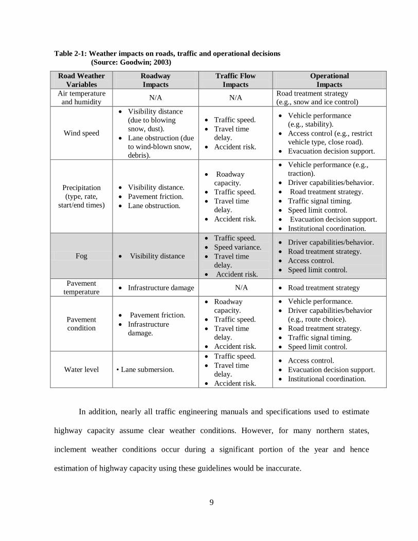
Goodwin (2003) summarized the impacts of various weather events on roadways, traffic

flow, and operational decisions (as shown in Table 2-1).

9

Table 2-1: Weather impacts on roads, traffic and operational decisions (Source: Goodwin; 2003)

Road Weather Variables

Roadway Impacts

Traffic Flow Impacts

Operational Impacts

Air temperature and humidity N/A N/A Road treatment strategy

(e.g., snow and ice control)

Wind speed

• Visibility distance (due to blowing snow, dust).

• Lane obstruction (due to wind-blown snow, debris).

• Traffic speed. • Travel time

delay. • Accident risk.

• Vehicle performance (e.g., stability).

• Access control (e.g., restrict vehicle type, close road).

• Evacuation decision support.

Precipitation (type, rate,

start/end times)

• Visibility distance. • Pavement friction. • Lane obstruction.

• Roadway capacity.

• Traffic speed. • Travel time

delay. • Accident risk.

• Vehicle performance (e.g., traction).

• Driver capabilities/behavior. • Road treatment strategy. • Traffic signal timing. • Speed limit control. • Evacuation decision support. • Institutional coordination.

Fog • Visibility distance

• Traffic speed. • Speed variance. • Travel time

delay. • Accident risk.

• Driver capabilities/behavior. • Road treatment strategy. • Access control. • Speed limit control.

Pavement temperature • Infrastructure damage N/A • Road treatment strategy

Pavement condition

• Pavement friction. • Infrastructure

damage.

• Roadway capacity.

• Traffic speed. • Travel time

delay. • Accident risk.

• Vehicle performance. • Driver capabilities/behavior

(e.g., route choice). • Road treatment strategy. • Traffic signal timing. • Speed limit control.

Water level • Lane submersion.

• Traffic speed. • Travel time

delay. • Accident risk.

• Access control. • Evacuation decision support. • Institutional coordination.

In addition, nearly all traffic engineering manuals and specifications used to estimate

highway capacity assume clear weather conditions. However, for many northern states,

inclement weather conditions occur during a significant portion of the year and hence

estimation of highway capacity using these guidelines would be inaccurate.

10

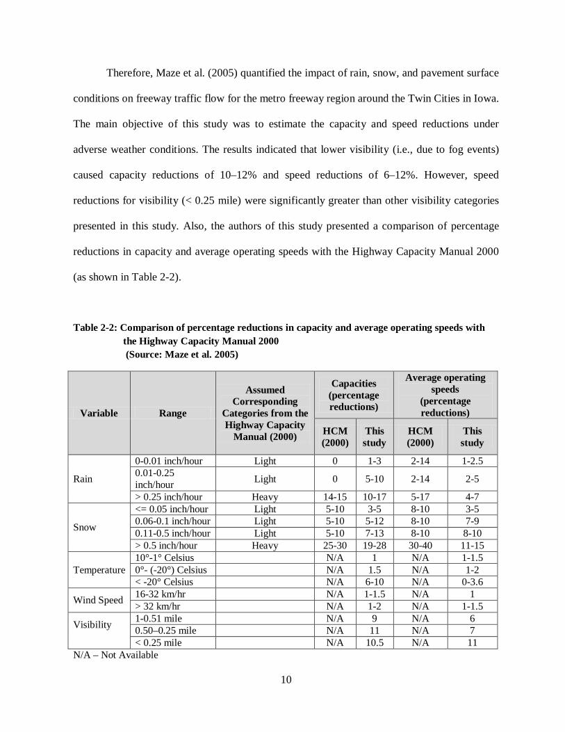
Therefore, Maze et al. (2005) quantified the impact of rain, snow, and pavement surface

conditions on freeway traffic flow for the metro freeway region around the Twin Cities in Iowa.

The main objective of this study was to estimate the capacity and speed reductions under

adverse weather conditions. The results indicated that lower visibility (i.e., due to fog events)

caused capacity reductions of 10–12% and speed reductions of 6–12%. However, speed

reductions for visibility (< 0.25 mile) were significantly greater than other visibility categories

presented in this study. Also, the authors of this study presented a comparison of percentage

reductions in capacity and average operating speeds with the Highway Capacity Manual 2000

(as shown in Table 2-2).

Table 2-2: Comparison of percentage reductions in capacity and average operating speeds with the Highway Capacity Manual 2000 (Source: Maze et al. 2005)

Variable Range

Assumed Corresponding

Categories from the Highway Capacity

Manual (2000)

Capacities (percentage reductions)

Average operating speeds

(percentage reductions)

HCM (2000)

This study

HCM (2000)

This study

Rain

0-0.01 inch/hour Light 0 1-3 2-14 1-2.5 0.01-0.25 inch/hour Light 0 5-10 2-14 2-5

> 0.25 inch/hour Heavy 14-15 10-17 5-17 4-7

Snow

<= 0.05 inch/hour Light 5-10 3-5 8-10 3-5 0.06-0.1 inch/hour Light 5-10 5-12 8-10 7-9 0.11-0.5 inch/hour Light 5-10 7-13 8-10 8-10 > 0.5 inch/hour Heavy 25-30 19-28 30-40 11-15

Temperature 10°-1° Celsius N/A 1 N/A 1-1.5 0°- (-20°) Celsius N/A 1.5 N/A 1-2 < -20° Celsius N/A 6-10 N/A 0-3.6

Wind Speed 16-32 km/hr N/A 1-1.5 N/A 1 > 32 km/hr N/A 1-2 N/A 1-1.5

Visibility

1-0.51 mile N/A 9 N/A 6 0.50–0.25 mile N/A 11 N/A 7 < 0.25 mile N/A 10.5 N/A 11

N/A – Not Available

11

Maze et al. (2006) reviewed prior studies that investigated weather’s impact on traffic

demand, traffic safety, and traffic flow characteristics. The findings pointed out that weather

conditions have an important impact on traffic safety, traffic demand, and traffic flow. In

addition, it was found that roadway traffic volumes reduced by less than 5% during rainstorms,

and from 7 to 80% for snowstorms. The results of this study indicated also that road weather

information systems (RWIS) are very beneficial tool for traffic management.

Pisano and Goodwin (2004) reported the impacts of inclement weather on traffic flow

and described an emerging concept of operations for a system-wide approach to traffic

management in adverse weather to assess weather’s impacts and implement operational

strategies that improve safety, mobility, and productivity. They stated the required future

research that is needed in order to apply the weather-responsive traffic management. They also

highlighted the concept of operation by the following questions.

• What data, processes, and procedures are needed by traffic managers to support

weather-responsive traffic management?

• How should weather-related data, processes, and procedures be integrated with

other transportation management systems and activities?

• What additional resources are needed to support weather-responsive traffic

management?

2.1.2 Impacts on Traffic Safety

Most of earlier studies that studied weather impacts on traffic safety such as McBride et

al. (1977), Brodsky and Hakkert (1988), Perry and Symons (1991), Savenhed (1994), Shankar

et al. (1995), Scharsching (1996), Brow and Baass (1997), Khattak et al. (1998, 2000),

12

Norrman et al. (2000), and Eissenberg (2004), showed that crash rates increase during

inclement weather such as fog, rain, snow, storm, high winds and as roadways became wet or

snow or ice-covered.

Maze et al. (2006) indicated that during reduced visibility conditions (<0.25 mile) and

high wind speeds (> 40 miles per hour), crash rates increased to about 25 times the normal

crash rate.

Edwards (1996) examined the spatial dimension of weather-related road crashes using

data extracted from police crash report forms. A comparison between frequency of crash

occurrence and weather conditions across England and Wales was done. The main finding from

this study was that the reporting of crashes in hazardous weather broadly follows the regional

weather patterns for those hazards.

Lynn et al. (2002) studied fog-related crashes on the Fancy Gap and Afton Mountain

sections of I-64 and I-77 in Virginia because these interstates have a long history of fog-related

crashes. The main objective of this study was to evaluate the nature and severity of the problem

of fog-related crashes in this area, to identify alternative solutions and technologies to address

the problems. The primary recommendations from this study were to install variable message

signs (VMS) to warn drivers of fog-related vehicle stops or slowdowns and to use highway

advisory radio within the fog zone to communicate with drivers.

Less effort has been devoted to explore how weather-related risks vary over time, and

what these variations inform us about interactions between weather and other risk factors. In

this regard, Andrey et al. (2003) examined temporal variations in weather-related collision and

injury risk using collision and weather data for Ottawa, Canada over the period 1990-1998. In

this study, to estimate and compare the risk of collision and injury during precipitation, a

13

matched-pair approach was used to define precipitation events and corresponding controls. The

findings revealed that collision crash risk increased significantly-by about 50% for winter

precipitation and by more than 100% for rain. In addition, collision risks were high during the

early winter season and on weekends compared to weekdays.

2.2 Drivers’ Response to Reduced Visibility Conditions

Drivers’ responses to both traffic and environmental conditions can be examined

through a variety of approaches, including questionnaire surveys, driving simulator

experiments, and network monitoring. The relatively low cost of questionnaire surveys,

compared to the other approaches, has encouraged researchers to use it as a way to collect data

on different driving situations under different traffic and environmental conditions (Chatterjee

et al., 2002).

2.2.1 Using Questionnaire Surveys

In general, there are two kinds of questionnaires: a stated preference (SP) survey,

examining human response to a hypothetical situation, and a revealed preference (RP) survey,

investigating human response derived from a real-life choice situation in the physical world.

The primary shortcoming of SP data is that they might not be harmonious with actual behavior.

A number of prior studies examined consistency between RP and SP data. By

comparing SP data to actual trip data, Loomis (1993) found that SP relating to intended trips

under alternative quality levels are valid and reliable indicators of actual behavior. Cumming et

al. (1995) compared real purchasing behavior for private goods with dichotomous choice (DC)

14

contingent valuation questions. They found that the proportion of DC “yes” responses exceeds

the proportion of actual purchases. Also, Johannesson et al. (1998) showed that hypothetical

"yes" responses overestimate the real purchases.

Yannis et al. (2005) indicated that some participants may have the tendency to

exaggerate when they respond to SP questions and hence, more attention should be given to the

results explanation and conclusions.

Despite those drawbacks, questionnaire surveys have been commonly used so far to

study drivers’ responses to Advanced Traveler Information System (ATIS) and to adverse

weather conditions. Clearly, the surveys can provide valid results and indications. However,

actual magnitude of these results should be viewed carefully and interpreted conservatively.

The SP surveys have been widely adopted in numerous transportation studies. Abdel-

Aty et al. (1994), Khattak et al. (1996), Mahmassani et al. (2003), Iragüen and Ortúzar (2004),

Tilahun et al. (2007), Junyi et al. (2008), Carlsson et al. (2010) and Correia and Viegas (2011)

used SP method to identify the behaviors of drivers with ATIS deployments.

2.2.1.1 Drivers’ responses to ATIS

Many previous studies focused on studying commuters’ responses and satisfactions

with traveler advisory systems such as variable message signs.

Haselkorn et al. (1989) examined the influence of traffic information from commercial

radio, television traffic announcements, DMS, highway advisory radio and telephone

information services on driver departure time and route choice behavior. A driver mail-back

survey was undertaken in Seattle in September 1988. A total of 3893 participants sent complete

responses (40% response rate). Using principal components factor analysis, it was found that

15

commuting distance and time characteristics, attitudes towards different sources of traffic

information (radio–based, television, DMS, etc) and commuter characteristics were the

components related to route choice.

Harris and Konheim (1995) surveyed 1002 peak-hour travelers in the New York

metropolitan area to investigate driver’s satisfaction with ATIS. The findings revealed that

approximately 88% of the drivers believe that ATIS are important in providing information

about location and duration of delays and alternative route travel times. In addition 78% of

commuters were willing to pay for ATIS.

In addition, using a questionnaire survey, Benson (1996) investigated drivers’ behaviors

when they encounter Dynamic Message Signs (DMSs). He examined whether drivers noticed

and therefore comply with DMSs, The findings revealed that approximately 20% out of 500

respondents ignored DMSs instructions while driving.

Emmerink et al. (1996) surveyed road users in the Amsterdam corridor (on the ring

road’s access motorways A1, A2 and A4) in July 1994 to examine the impact of both radio

traffic information and VMS information on route choice behavior. 2145 questionnaires were

distributed among drivers however, only 826 of them were returned (response rate: 38.6%).

Discrete choice models were conducted to investigate the factors that influence route choice

behavior. The results revealed that women were less likely to be influenced by traffic

information and the impacts of both radio traffic information and VMS information on route

choice behavior were very similar. In addition, the results indicated that there is a positive

correlation between the use of radio traffic information and VMS information.

Chatterjee et al. (2002) conducted SP questionnaires to study driver response to VMS in

London. The main objective of this study was to investigate the effect of different messages

16

displayed on VMS on route choice. Three questionnaires were conducted in this study. The first

questionnaire focused on studying drivers’ attitudes to London VMS information. However, the

second questionnaire investigated how drivers would respond to different VMS messages.

Logistic regression models were developed to predict the probability of diversion in response to

different VMS messages. The third questionnaire was conducted during the activation of an

immediate warning message. The results showed that one third of motorists saw the

information that was displayed on VMS however, few of them diverted.

Zwahlen and Russ (2002) evaluated a real-time travel time prediction system (TIPS) in

a construction work zone that includes CMS. The main aim was to evaluate the travel time and

distance to the end of the work zone displayed on CMS to motorists. They surveyed the

motoring public regarding their acceptance of this system. A total of 660 completed surveys

were returned and analyzed (21% response rate). 97% of surveyed motorists indicated that

TIPS that provide real-time travel time information in advance of work zones and in advance of

open exit ramps is either outright helpful or maybe helpful.

Al-Deek et al. (2003) investigated predictive information on traveler behavior using

Computer Assisted Telephone Interview (CATI) and web-based (online) survey. A total of 400

and 439 responses were collected using the CATI and web-bases surveys, respectively. The

results showed that crash location and expected delay were the most needed information by

drivers.

Lai and Yen (2004) examined how DMS affected driver behavior such as changing

lanes, route changing, and decreasing speed using a questionnaire survey. 312 respondents

participated in the survey. The main results showed that gender, age, and education were the

most significant factors affecting drivers’ preference for DMS. Drivers also were asked about

17

their preference of color, and display formats of DMS. The analysis of survey revealed red and

orange colors as well as flashing formats for the messages were preferred by most of

participants.

Peeta and Ramos (2006) examined commuters’ responses to traffic information

provided through DMS using a SP survey using three different administration methods: an on-

site survey, a mail-back survey, and an Internet-based survey. The findings showed that a

combination of survey administration methods may generate more representative data. In

addition, the results showed that a high correlation between DMS message type and driver

response was existed.

In addition, a number of earlier studies have used images of CMS to explore driver

comprehension and responses to the information displaying on CMS. For instance, using a SP

survey, Wardman et al. (1997) evaluated the effect of information provided by CMS on drivers’

route choice. Lai and Wong (2000) examined driver comprehension of the traffic information

presented on CMS.

Moreover, using laptop computers, Dudek and Ullman (2002) investigated the effect of

flashing an entire message, flashing one line and alternating text on one line on drivers’

comprehension and recall. Using driving simulation experiments, Wang and Cao (2005)

studied the influences of CMS format and number of message lines on drivers’ response time.

Dudek et al. (2006) examined the effect of displaying CMS with dynamic features on drivers’

comprehension and response time. Ullman et al. (2007) investigated the ability of motorists to

capture and process information on two CMS used in sequence. Finally, Lai (2010) examined

the effects of color scheme and message lines of CMS on driver performance.

18

2.2.1.2 Drivers’ responses to inclement weather

Noticeably, very few prior studies examined drivers’ behavior in adverse weather

conditions such as rain, snow, fog/smoke using questionnaire surveys.

Kilpelainen and Summala (2007) examined the effects of adverse weather and traffic

weather forecasts on driver behavior in Finland using a questionnaire on perceptions of

weather, pre-trip acquisition of weather information, and possible changes in travel plan. The

questionnaire was conducted in rural service stations in different weather and driving

conditions. The questionnaires were distributed and instantaneously collected. A total of 1437

complete questionnaires were collected and analyzed. Drivers were asked to rate the current

driving conditions on a three steps scale (normal, bad, very bad), classify the slipperiness on a

five-step scale (ranging from very slippery to not slippery), to mention whether they had

acquired weather-related information for the trip, to report their decisions before and during the

trip, and to estimate their speed, headways and overtaking frequency compared to those on the

same road in good weather and driving conditions. The authors also collected data from traffic

weather forecasts, weather measurement stations, and automatic traffic counters concerning the

same area/road. The findings revealed that drivers, who had acquired information, had also

made more changes to travel plans. On the other hand, they estimated prevailing risks higher

than those who did not receive weather information. The results suggest that drivers’ behavior

is basically affected by the prevailing observable conditions rather than traffic weather

forecasts.

19

2.2.2 Using Driving Simulator Experiments

Driving Simulators have been used in many prior studies as it is a very economical and

a safer option compared to field studies. Driving simulators have been used on a broad variety

of experiments where most of them focused on studying drivers’ behavior under conditions that

will not be safe to test in the real world.

Ng and Mannering (1998) developed a driving simulator experiment that collected data

from four different advisory scenarios: 1) in-vehicle information (they called this type of

information IVD); 2) out of vehicle information (VMS); 3) combination of in-vehicle and out

of vehicle; and 4) No information present. Furthermore, there were three main messages

viewed by the subjects that drove the VMS or IVD scenario: 1) fog ahead – slow down 45 mph;

2) curvy road – drive slowly; and 3) snow plow ahead – 35 mph. Static speed limit signs

showed a maximum of 65 mph. In addition, two types of weather conditions (fog and no fog)

and two types of incidents (snowplows or no snowplows) were incorporated for each sign.

The authors did find statistical differences in the average speed when fog or snowplows

were present. Moreover, they discovered that the subjects that drove the “no sign” condition

presented higher speeds than the ones that drove a sign condition.

Ikeda et al. (2002) examined whether factors like vision, visual perception, cognition,

reaction time, and driving knowledge were affected by the drivers’ age. Twelve subjects

participated in the driving experiment where they were asked to follow traffic signals and signs

and preceding cars during a 2 km stretch. It was found that depending on age, drivers have

reaction times of 0.3 and 0.42 seconds. Also, the required time for judgment and recognition of

another vehicle for older drivers is shorter than the one for younger drivers. Due to

20

deterioration of information processing caused by aging, older drivers are not good at

processing multiple tasks, but they are faster than young drivers at recognizing individual tasks.

Dudek et al. (2005) conducted driving simulator study to examine the effects on

motorists of the following three types of CMS dynamic display features: 1) flashing an entire

one-phase message; 2) flashing one line of a one-phase message; and 3) alternating text on one

line of a three-line CMS while keeping the other two lines of text constant on the second phase

of the message thus displaying redundant information. The results indicated that flashing

messages may have an adverse effect on message comprehension for unfamiliar drivers.

Mitchell et al. (2005) investigated the use of a driving simulator to evaluate the

effectiveness of traffic safety countermeasures such as reduced speed limit signs, rumble strips,

and reduced lane width in freeway work zones. The main finding of this study was that a

narrow traffic lane appeared to be effective in reducing average speeds through the work zone

when compared to the base scenario (no countermeasures). However, the placement of rumble

strips was effective in reducing average speeds only in the transition area.

Dudek et al. (2006) employed a driving simulator experiment to evaluate flashing

message features on VMS. The results indicated that no differences in the average reading time

between the two types of display and among age groups, education levels, and gender were

observed. However, a flashing message might not provide the same effect as the static message

when unfamiliar drivers read the message.

Broughton et al. (2007) examined factors that govern car following under conditions of

reduced visibility due to fog. Using a driving simulator, the behavior of drivers following a lead

vehicle at 13.4 m/s (30 mph) or 22.4 m/s (50 mph) under three visibility conditions (clear or

one of two densities of simulated fog) were observed. The results revealed that many drivers

21

strive to maintain visible contact with the lead vehicle when driving through dense fog

however; headway time might be too short for adequate safety. In addition, they indicated that

even drivers who do not maintain visual contact with the lead vehicle may still constitute a

hazard for following drivers who seek to maintain visible contact with them by following too

closely. Finally, they suggested that a built-in vehicle’s device that provides the driver with a

substitute visual image would mitigate the unsafe headway times necessary to maintain visual

contact.

Reimer et al. (2007) explored the effects of age, gender, and time of day on drivers’

performance using a driving simulation experiment. The results revealed that time of day, age,

and gender significantly affected drivers’ speed. In the late afternoon period, drivers drove

significantly slower than drivers in other time periods. Moreover, it was found that old females

(50 years old or more) tended to driver more slowly. In addition, time of day and age affected

driver’s speed and reaction time however; gender did not show significant effects.

Andersen et al. (2008) examined the effects of reduced visibility of scene information

from fog on car following performance using a driving simulator. The main finding from this

study was that the presence of fog in a car following task has a greater effect on responding to

variations in speed rather than variations in headway distance.

22

2.2.3 Using Field Experiments

Many prior research efforts investigated drivers’ responses to adverse weather

conditions such as reduction in visibility due to FS by observing traffic spot speeds such as

Hogema and Horst (1997), Edwards (1999), Maze et al. (2006) and MacCarley et al. (2006).

For example, Hogema and Horst (1997) evaluated the Dutch fog warning system in

terms of driving behavior for a period of more than 2 years after implementing the system. The

results showed that the system has a positive effect on speed choice in fog as it resulted in a

decrease of speed of about 8 to 10 kph.

MacCarley et al. (2006) examined drivers’ responses to messages displayed by a CMS

warning of fog ahead and advising specific speeds at lower visibility levels. The speed, length

and time of detection were individually recorded for all vehicles over a two-year period of

study at four sites: two prior to exposure to the CMS, and two after exposure to the CMS. The

results indicated that the mean speed decreased by an average of 1.1 mph compared with the

mean speed of traffic in the absence of a message.

23

2.3 Existing Visibility warning Systems

Nowadays, there are many fog warning systems to warn drivers of sudden drops in

visibility especially due to fog. This section presents a literature review for the existing fog

warning and detection systems.

2.3.1 Projects in USA

2.3.1.1 Alabama DOT low visibility warning system

In fall 1999, the Alabama Department of Transportation (DOT) deployed a low

visibility warning system on a prone fog area near Mobile, Alabama (Goodwin 2003). This

system consisted of 6 visibility sensors with forward-scatter technology that were installed at

about one-mile (1.6-kilometer) intervals. About 25 Closed Circuit Television (CCTV) cameras

were used for monitoring traffic data. Via a fiber optic cable communication system, field

sensor data were transmitted to a central computer in the control room. Also to display

advisories or regulations to drivers, 24 VSL and 5 DMS signs were used. Operators displayed

messages on DMS and changed speed limits with VSL based on the current visibility

conditions (as shown in Table 2-3).

Goodwin (2003) indicated that Alabama’s low visibility system was effective in

improving safety, reducing average speed and minimizing crash risk in low visibility condition.

24

Table 2-3: Alabama DOT low visibility warning system strategies (Source: Goodwin; 2003)

Visibility Distance Advisories on DMS Other Strategies Less than 900 feet (274.3 meters) “FOG WARNING” Speed limit at 65 mph (104.5 kph)

Less than 660 feet (201.2 meters)

“FOG” alternating with “SLOW, USE LOW BEAMS”

• “55 MPH” (88.4 kph) on VSL signs • “TRUCKS KEEP RIGHT” on DMS

Less than 450 feet (137.2 meters)

“FOG” alternating with “SLOW, USE LOW BEAMS”

• “45 MPH” (72.4 kph) on VSL signs • “TRUCKS KEEP RIGHT” on DMS

Less than 280 feet (85.3 meters)

“DENSE FOG” alternating with “SLOW, USE LOW BEAMS”

• “35 MPH” (56.3 kph) on VSL signs • “TRUCKS KEEP RIGHT” on DMS • Street lighting extinguished

Less than 175 feet (53.3 meters)

I-10 CLOSED, KEEP RIGHT, EXIT ½ MILE

Road Closure by Highway Patrol

2.3.1.2 California DOT motorist warning system

In 1996, California Department of Transportation (Caltrans), District 10, implemented a

low visibility warning system to warn drivers of adverse visibility on I-5, Stockton, CA. To

collect traffic and weather data, the system includes 36 traffic speed monitoring sites, 9

complete Environmental Sensor Stations (ESS), and 9 DMS for warning drivers (see Table 2-

4).

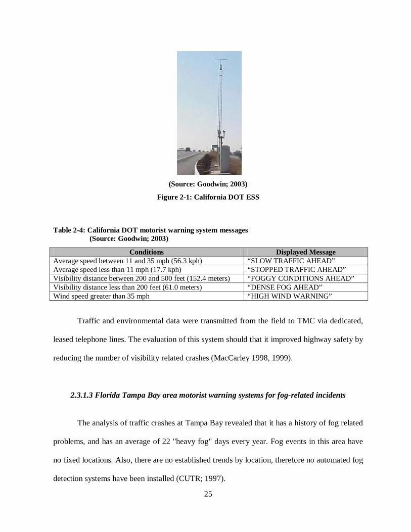
Figure 2-1 shows one of the California’s ESS. Each ESS includes a forward-scatter

visibility sensor, a rain gauge, wind speed and direction sensors, a relative humidity sensor, a

thermometer, a barometer, and a remote processing unit (Goodwin; 2003).

25

(Source: Goodwin; 2003)

Figure 2-1: California DOT ESS

Table 2-4: California DOT motorist warning system messages (Source: Goodwin; 2003)

Conditions Displayed Message Average speed between 11 and 35 mph (56.3 kph) “SLOW TRAFFIC AHEAD” Average speed less than 11 mph (17.7 kph) “STOPPED TRAFFIC AHEAD” Visibility distance between 200 and 500 feet (152.4 meters) “FOGGY CONDITIONS AHEAD” Visibility distance less than 200 feet (61.0 meters) “DENSE FOG AHEAD” Wind speed greater than 35 mph “HIGH WIND WARNING”

Traffic and environmental data were transmitted from the field to TMC via dedicated,

leased telephone lines. The evaluation of this system should that it improved highway safety by

reducing the number of visibility related crashes (MacCarley 1998, 1999).

2.3.1.3 Florida Tampa Bay area motorist warning systems for fog-related incidents

The analysis of traffic crashes at Tampa Bay revealed that it has a history of fog related

problems, and has an average of 22 "heavy fog" days every year. Fog events in this area have

no fixed locations. Also, there are no established trends by location, therefore no automated fog

detection systems have been installed (CUTR; 1997).

26

2.3.1.4 Georgia automated adverse visibility warning and control system

In 2001, at a site known for fog problems on Interstate Highway 75 in South Georgia,

Georgia Tech and the Georgia Department of Transportation (GDOT) jointly implemented an

automated adverse visibility warning and control system along 14 miles section of I-75 to warn

drivers about adverse visibility conditions.

This system consists of 19 visibility sensors, 2 DMSs, and 5 sets of traffic loops

monitor speed and headway for northbound and southbound moving traffic lanes. The data

collected by sensors are transmitted to an on-site computer using a fiber-optic communications

network. The total project cost for system development and installation was $4 million. In

addition, the cost needed to duplicate the system would be approximately $1.7 million

(Gimmestad et al. 2004).

2.3.1.5 Idaho DOT motorist warning system

Between 1988 and 1993, 18 low visibility related crashes, involving 91 vehicles and

resulting in 9 fatalities and 46 injuries, occurred on a 45-mile stretch of Interstate 84 in

southeast Idaho. Therefore, in 1993, to improve the safety in this area, Idaho Transportation

Department (ITD) installed weather and visibility warning system at that site to measure three

kinds of data: traffic, visibility, and weather data. Furthermore, to measure driver behavior

during normal clear days and visibility event periods, automatic traffic counters were used to

observe and record the lane number, time, speed, and length of each vehicle passing by the

sensor site (Goodwin; 2003).

The system consists of three visibility sensors (as shown in Figure 2-2) to measure

reduced visibility conditions and a video camera to provide visual verification of the visibility

27

sensors. The data collected by these sensors are transmitted to a master computer which records

readings every five minutes. This project was conducted in two phases. The objective of phase

I was to determine if the visibility sensors provide accurate visibility measurements, while the

objective of Phase II was to assess whether the VMSs would reduce vehicle speed during

periods of low visibility (Kyte et al. 2000).

(Source: Goodwin; 2003)

Figure 2-2: Idaho DOT visibility sensor

In this regards, Liang et al. (1998) studied the effects of visibility and other

environmental factors on driver speed. The main objective was to determine the efficacy of

using Idaho visibility warning System to warn motorists of inclement weather conditions and to

quantify the nature of the speed-visibility relationship.

The results indicated that drivers respond to adverse environmental conditions by

reducing their speeds by about 5.0 mph during the fog events and approximately 12 mph during

the snow events (Table 2-5). Also, it was found that the primary factors affecting driver speed

were reduced visibility and winds exceeding 25 mph. Also, Table 2-6 indicates an initial set of

recommended speed levels based on the findings of the aforementioned study.

28

Table 2-5: Vehicle speed characteristics (mph) (Source: Liang et al. 1998)

Number of Events

Evaluated

Car/trucks Combined

Passenger Cars Only Trucks only

Mean Speed

Standard Deviation

Mean Speed

Standard Deviation

Mean Speed

Standard Deviation

Base Conditions 3 65.8 2.3 68.4 3.6 63.5 2.6 Fog Events 2 60.8 4.6 64.8 7.2 59.2 4.4 Snow Events 11 53.9 6.3 55.3 7.6 52.5 6.4 Table 2-6: An initial set of recommended speeds (mph)

(Source: Liang et al. 1998)

Visibility (miles) Night Time Speed Day Time Speed 0-1 60 62 >1 63 64

2.3.1.6 Maryland I-68 fog detection system

In 2005, a Fog detection system was installed on I-68, Big Savage Mt. The system

consists of 4 ground mounted signs with solar powered flashers, 2 upgraded RWIS (camera,

radio, remote processing unit, fog sensor), 6 Yagi directional antennas, 3 Omni directional

antennas, and10 Spread – spectrum radios (shelf item) (Sabra, Wang & Associates 2003).

2.3.1.7 South Carolina DOT low visibility warning system

In 1992, South Carolina Department of Transportation (DOT) deployed a low visibility

warning system on 7 miles (11.3 kilometers) on Interstate 526 to warn drivers of dense fog

conditions, reduce traffic speeds, and guide vehicles safely through this fog-prone area.

The system consisted of 5 forward-scatter visibility sensors spaced at 500-foot (152.4

meter intervals, pavement lights installed at 110-foot spacing (33.5 meter), adjustable street

29

light controls, 8 closed circuit television cameras, 8 DMSs, a remote processing unit, a central

control computer, and a fiber optic cable communication system. Table 2-7 shows the advisory

and control strategies of the system. The South Carolina low visibility warning system

improved both mobility and safety on I-526. No fog-related crashes have occurred since the

system was deployed (Goodwin; 2003, Schreiner; 2000, and Center for Urban Transportation

Research; 1997).

Table 2-7: South Carolina DOT low visibility warning system strategies (Goodwin 2003)

Visibility Conditions

Advisory Strategies

Control Strategies

700 to 900 feet (213.4 to 274.3 meters)

“POTENTIAL FOR FOG” and “LIGHT FOG CAUTION” on DMS

“LIGHT FOG TRUCKS 45 MPH” and “TRUCKS KEEP RIGHT” on DMS

450 to 700 feet (137.2 to 213.4 meters)

“FOG CAUTION” and “FOG REDUCE SPEED” on DMS

Pavement lights illuminated “FOG REDUCE SPEED 45 MPH” and “TRUCKS KEEP RIGHT” on DMS

300 to 450 feet (91.4 to 137.2 meters) “FOG CAUTION” on DMS

Pavement lights illuminated and overhead street lighting extinguished “FOG REDUCE SPEED 35 MPH” and “TRUCKS KEEP RIGHT” on DMS

Less than 300 feet N/A

Pavement lights illuminated and overhead street lighting extinguished “DENSE FOG REDUCE SPEED 25 MPH” and “TRUCKS KEEP RIGHT” on DMS If warranted, “PREPARE TO STOP”, “I-526 BRIDGE CLOSED AHEAD USE I 26/US 17”, and “ALL TRAFFIC MUST EXIT” on DMS

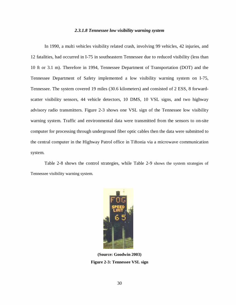
30

2.3.1.8 Tennessee low visibility warning system

In 1990, a multi vehicles visibility related crash, involving 99 vehicles, 42 injuries, and

12 fatalities, had occurred in I-75 in southeastern Tennessee due to reduced visibility (less than

10 ft or 3.1 m). Therefore in 1994, Tennessee Department of Transportation (DOT) and the

Tennessee Department of Safety implemented a low visibility warning system on I-75,

Tennessee. The system covered 19 miles (30.6 kilometers) and consisted of 2 ESS, 8 forward-

scatter visibility sensors, 44 vehicle detectors, 10 DMS, 10 VSL signs, and two highway

advisory radio transmitters. Figure 2-3 shows one VSL sign of the Tennessee low visibility

warning system. Traffic and environmental data were transmitted from the sensors to on-site

computer for processing through underground fiber optic cables then the data were submitted to

the central computer in the Highway Patrol office in Tiftonia via a microwave communication

system.

Table 2-8 shows the control strategies, while Table 2-9 shows the system strategies of

Tennessee visibility warning system.

(Source: Goodwin 2003)

Figure 2-3: Tennessee VSL sign

31

Table 2-8: Control strategies of Tennessee low visibility warning system (Source: Dahlinger et al. 2001)

Visibility Distance Control strategies From 480 feet (146.3 kph) to 1,320 feet The speed limit is reduced from 65 to 50 mph From 240 to 480 feet. The speed limit is lowered to 35 mph (56.3 kph) Less than 240 feet or 73.2 meters Road close due to Fog

Table 2-9: System strategies of Tennessee low visibility warning system (Source: Dahlinger et al. 2001)

Conditions Advisories on DMS Other Strategies Speed

Reduced “CAUTION” alternating with “SLOW TRAFFIC AHEAD” N/A

Fog Detected “CAUTION” alternating with “FOG AHEAD TURN ON LOW BEAMS” • “FOG” displayed on VSL signs

Speed Limit Reduced

“FOG AHEAD” alternating with “ADVISORY RADIO TUNE TO XXXX AM” • “FOG” & Reduced Speed Limits

displayed on VSL signs • HAR messages broadcasted

“FOG AHEAD” alternating with “REDUCE SPEED TURN ON LOW BEAMS” “FOG” alternating with “SPEED LIMIT XX MPH”

Roadway Closed

“DETOUR AHEAD” alternating with “REDUCE SPEED MERGE RIGHT” • “FOG” displayed on VSL signs

• HAR messages broadcasted • Ramp Gates closed

“I-75 CLOSED” alternating with “DETOUR” “FOG AHEAD” alternating with “ADVISORY RADIO TUNE TO XXXX AM”

After deployment of the warning system in 1994, safety improved significantly as only

one visibility related crash has occurred due to fog (Dahlinger et al. 1995, 2001), (Tennessee

ITS State Status Report 2000).

2.3.1.9 Utah DOT low visibility warning system

In 1988 there was a 66 multi-vehicles crash and in 1991 ten crashes, with three

fatalities, occurred on one day due to dense fog on Interstate 215 above the Jordan River in Salt

Lake City, Utah. Therefore, during 1995 and 2000, the Utah Department of Transportation

32

(DOT) deployed a low visibility warning system on two mile (three-kilometer) of Interstate 215

to notify drivers of safe travel speeds and to achieve more uniform traffic flow in cases of

reduction of visibility.

The warning system consisted of 4 forward-scatter visibility sensors and 6 vehicle

detection sites to collect data on prevailing conditions. The speed, length, and lane of each

vehicle were measured by underground loop detectors. Traffic and Environmental data were

transmitted to a central computer through Ultra-High Frequency radio modems. In addition,

two DMS were used to post advisories to drivers. Table 2-10 shows Utah DOT low visibility

warning system messages (Perrin et al. 2000, 2002).

Table 2-10: Utah DOT low visibility warning system messages (Source: Perrin et al. 2000)

Visibility Conditions Displayed Messages 656 to 820 feet (200 to 250 meters) “FOG AHEAD” 492 to 656 feet (150 to 200 meters) “DENSE FOG” alternating with “ADVISE 50 MPH” 328 to 492 feet (100 to 150 meters) “DENSE FOG” alternating with “ADVISE 40 MPH” 197 to 328 feet (60 to 100 meters) “DENSE FOG” alternating with “ADVISE 30 MPH” Less than 197 feet (60 meters) “DENSE FOG” alternating with “ADVISE 25 MPH”

Perrin et al. (2002) evaluated Utah low visibility warning system in reducing the

variation between speeds which is the most important factor in reducing fog-related crashes. To

achieve this goal, they tested a fog-prone area of I-215 in Salt Lake City, Utah, during three

phases. Phase I was the base case, no VMSs were used in this phase. In phase II, the warning

system was implemented and VMSs were used. Phase III data was collected following VMS

installation during the winter of 1999-2000. The displayed VMSs, based on measured visibility,

are listed below in Table 2-11.

The results of this research showed that Utah warning system successfully reduced

speed variation by an average 22%. This finding supports a prior idea that informing drivers of

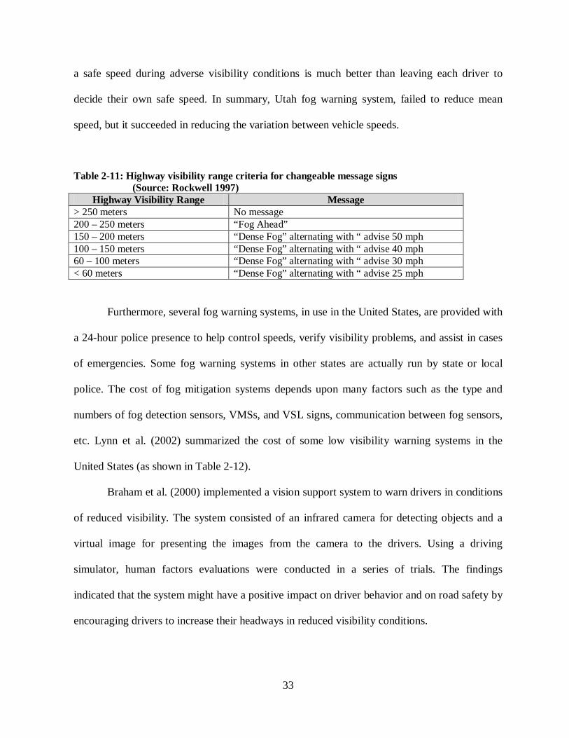
33

a safe speed during adverse visibility conditions is much better than leaving each driver to

decide their own safe speed. In summary, Utah fog warning system, failed to reduce mean

speed, but it succeeded in reducing the variation between vehicle speeds.

Table 2-11: Highway visibility range criteria for changeable message signs (Source: Rockwell 1997)

Highway Visibility Range Message > 250 meters No message 200 – 250 meters “Fog Ahead” 150 – 200 meters “Dense Fog” alternating with “ advise 50 mph 100 – 150 meters “Dense Fog” alternating with “ advise 40 mph 60 – 100 meters “Dense Fog” alternating with “ advise 30 mph < 60 meters “Dense Fog” alternating with “ advise 25 mph

Furthermore, several fog warning systems, in use in the United States, are provided with

a 24-hour police presence to help control speeds, verify visibility problems, and assist in cases

of emergencies. Some fog warning systems in other states are actually run by state or local

police. The cost of fog mitigation systems depends upon many factors such as the type and

numbers of fog detection sensors, VMSs, and VSL signs, communication between fog sensors,

etc. Lynn et al. (2002) summarized the cost of some low visibility warning systems in the

United States (as shown in Table 2-12).

Braham et al. (2000) implemented a vision support system to warn drivers in conditions

of reduced visibility. The system consisted of an infrared camera for detecting objects and a

virtual image for presenting the images from the camera to the drivers. Using a driving

simulator, human factors evaluations were conducted in a series of trials. The findings

indicated that the system might have a positive impact on driver behavior and on road safety by

encouraging drivers to increase their headways in reduced visibility conditions.

34

Table 2-12: Cost of low visibility warning systems in the United States (Source: Lynn et al. 2002)

Location Length Visibility/Weather Detectors VMSs Traffic/Speed

Detectors Cost

I-10 (Mobile, Alabama) 6.2 miles 6 visibility sensors 4 VMSs, CCTV Loop detectors $18,000 excluding VMSs and loops

Rt. 99/I-5 (San Joaquin Valley, California) Unknown

15 Road Weather Information System (RWIS) stations, plus fog detectors, visibility test signs

80 VMSs None $3,600,000

I-5/Rt. 205 (Stockton, California) 16 miles 9 RWIS stations 9 VMSs 36 inductive loop

sensors $2,750,000 -- $2,770,000

Planned I-75 (Georgia / Florida border) 2 miles 19 visibility sensors Light emitting diode

(LED) VMSs 5 loop detectors $1,410,500

I-25 (Colorado) Unknown None, visibility reported by CDOT personnel

6 roadside VMSs, overhead VMSs None $275,000

I-69 (Fort Wayne, Indiana) ¾ mile 1 visibility sensor LED VMSs None $155,000 I-40 (Haywood County, North Carolina) 5 miles 3 visibility sensors 2 VMSs None $1,100,000

Rt. 22 (Crescent Mountain, Pennsylvania) 2 miles 1 RWIS VMSs, Highway

Advisory Radio None $411,010 plus $1,200,000 in upgrades

I-75 (Calhoun, Tennessee) 19 miles 8 fog detectors, 2 RWIS stations 20 VMSs 22 speed detectors $4,460,580

I-215 (Salt Lake City, Utah) Unknown 4 fog sensors 2 VMSs 6 loop detectors $461,000

35

2.3.2 Projects in England

In 1990, an automatic fog warning system (M25 London Automatic Fog-Warning

System) was designed by Traffic Control and Communications Division of the Department of

Transport, London. This system was installed on the M25 London orbital motorway to warn

drivers about formation of fog by displaying “Fog” legend on roadside matrix signals. Transport

Research Laboratory of the United Kingdom, evaluated the effectiveness of the system in

reducing the variation in vehicles’ speeds during inclement visibility conditions due to fog.

Based on data measured from 6 test sites, the results revealed that there was about a 1.8 mph

reduction in mean vehicle speeds when the signals were switched on (Cooper and Sawyer; 1993,

MacCarley; 1999).

2.3.3 Projects in the Netherlands

The Dutch Ministry of Transport implemented an automatic fog warning system to

achieve safer driving behavior during adverse visibility conditions along 12 km (7.4 mile)

section of the A16 Motorway in the Netherlands. The system consisted of 20 visibility sensors to

continuously measure the visibility distances. The objective of this system was to warn drivers of

reduced visibility conditions (i.e., due to fog) by displaying an explicit fog warning on overhead

matrix signs together with a maximum safe speed limit that depends on the actual measured

visibility distance.

Hogema and Horst (1997) evaluated the Dutch fog warning system in terms of driving

behavior for a period of more than 2 years after implementing the system. Using subsurface loop

detectors at six locations (four experimental and two control locations), continuous traffic

36

measurements for individual vehicles were observed. Data on the local visibility conditions and

on the messages displayed on the matrix signs were available on a 1-min basis. The results

showed that the system has a positive effect on speed choice in fog as it resulted in a decrease of

speed of about 8 to 10 kph.

2.3.4 Projects in Finland

Rama et al. (2000) investigated the effects of two VMS on driver behavior. The two signs

were a warning sign for slippery road conditions and a minimum headway sign. A before-and-

after experiment was performed at three test sites in Finland with an after period covering two

winter seasons. The slippery road condition sign decreased the mean speed on slippery roads by

1-2 km/h in addition to the decrease caused by the adverse road conditions. Moreover, the

minimum headway sign decreased the proportion of headways shorter than 1.5 s for cars in car-

following situations, in addition to a speed reduction of 1 km/h.

Luoma et al. (2000) indicated that the signs may have other effects on driver behavior

besides those measurable in terms of speed and headway that were found in Rama et al. (2000).

Therefore, this study was designed to investigate such potential effects. To achieve this goal, 114

drivers who had encountered the slippery road condition sign and 111 drivers who had

encountered the sign showing recommended minimum headway in adverse road surface

conditions were interviewed. The results indicated that these VMS have other effects, such as the

refocusing of attention to seek cues on potential hazards, testing the slipperiness of the road, and

more careful passing behavior.

37

2.3.5 Projects in Saudi Arabia

Al-Ghamdi (2004) evaluated the effectiveness of a fog detection and warning system on

driver behavior in terms of reduction in average speed, speed variability in the traffic stream, and

choice of time headway. This system was installed on a 2-km section of a two-lane, rural

highway in the Al-Baha region of Saudi Arabia. The system consisted of a visibility sensor, a

point detection device that utilizes infrared technology to measure visibility, and a VMS. In

addition, NC-97, an advanced traffic counter classifier, was used to measure traffic data (i.e.,

speed, headway, vehicle classification, and volume). Only one message was used during the

project and the VMS was activated once the sensor detects a reduction in visibility less than 200

m.

The main result from this study indicated the system was ineffective in reducing speed

variability. However, the system reduced mean speed throughout the experimental sections by

about 6.5 kph. On the other hand, this study had three drawbacks: (1) the frequency of the signs

within and before the fog-prone area was not tested, (2) no different messages and speeds were

tested, and (3) The distance from the sign at which drivers resume their normal speed was not

measured.

2.3.6 Summary of Existing Fog Warning Systems

Reviewing the existing visibility warning systems revealed that they have many

limitations. First, these systems were designed specifically for one road location (fixed systems)

and hence, it is not possible to reinstall them at other locations. Second, they are not cost-

effective in terms of system’s components, management and maintenance. Finally, most of them

38

depend on AC power supply and fiber-optic cable for internal communication thus; they are not

suitable in the absence of AC power. Therefore, there is a need to design a portable detection and

warning system that is developed from components that are inexpensive and available

commercially.

Chapter 3 presents the design and components of the portable visibility system that was

developed by researchers at UCF. A preliminary testing for the system’s performance is also

discussed and presented in Chapter 3.

2.4 Relationship between Crash Characteristics and Real-Time Traffic Flow variables

Subsurface loop detectors (LDs) are the most common freeway traffic surveillance

technologies used for various intelligent transportation system (ITS) applications such as travel

time estimation and crash detection. Recently, the emphasis in freeway management has been

shifting towards using LD data to develop real-time crash-risk assessment models.

Numerous studies have established statistical links between freeway crash risk and traffic

flow characteristics. However, there is a lack of good understanding of the relationship between

traffic flow variables (i.e. speed, volume and occupancy) and crashes that occur under reduced

visibility (visibility related crashes).

Earlier studies that examined relationships between traffic flow variables and crashes can

be categorized into two types; aggregate and disaggregate studies (Golob et al. 2004). Regarding

aggregate studies such as Zhou and Sisiopiku (1997), the units of analysis represent crash counts

or rates for specific time and location. For similar time and location, traffic flow is represented

by parameters of statistical distributions of traffic flow. Concerning disaggregate studies, the

39

units of analysis are individual crashes and traffic flow is represented by the corresponding

traffic flow variables at the same time and location of each crash (Golob et al. 2004).

In this regard, the relationship between historical crash occurrence and loop detectors

data gathered from stations surrounding the crash location have been explored by numerous

studies to develop crash prediction models. These models were developed by several of the

earlier studies such as Madanat and Liu (1995), Oh et al. (2001), Lee et al. (2002, 2003), Golob

and Recker (2003), Abdel-Aty et al. (2004, 2008), Abdel-Aty and Pande (2005), and Pande and

Abdel-Aty (2006).

Madanat and Liu (1995) used traffic stream and environmental conditions measured by

surveillance sensors for developing binary logit models. The objective was to estimate the crash

likelihood for two types of crashes, namely, crashes and overheating vehicles. The results

indicated that merging section, visibility, and rain were the significant variables affecting the

crash likelihood prediction.

Oh et al. (2001) used the Bayesian classifier to categorize the two possible traffic flow

conditions; crash versus normal traffic flow. The results showed that five minutes standard

deviation of 30-second speed measurements was the significant factor leading to crash

occurrence.

Lee et al. (2002) developed a log-linear model for predicting crashes using LD data. They

refined this model in a later study (Lee et al. 2003). The results revealed that the coefficient of

variation in speed (CVS) was the significant factor affecting the probability of crash occurrence.

In order to determine how crash characteristics are related to traffic flow conditions at the

time of occurrence, Golob and Recker (2003) developed a method involves nonlinear canonical

correlation applied together with cluster analyses. The results revealed that interactions between

40

traffic flow conditions and accident propensities vary with environmental factors. Twenty one

traffic flow regimes for three different ambient conditions were identified: eight regimes for dry

roads during daylight, six regimes for dry roads at night, and seven regimes for wet conditions

(based on condition of the roadway surface: wet or dry).

Abdel-Aty et al. (2004) adopted matched case-control logistic regression for developing a

crash likelihood prediction model using real-time traffic variables measured through serious of

LDs. The findings showed that the average occupancy observed at the upstream station along

with the CVS at the downstream station, both during 5-10 minutes prior to the crash, were the

significant factors affecting crash likelihood.

Abdel-Aty and Pande (2005) used Bayesian classifier based methodology, probabilistic

neural network to identify patterns in the freeway LDs data that potentially lead to traffic

crashes. The logarithm of CVS observed from the nearest station to the crash location and two

stations immediately preceding it upstream during 10-15 minutes prior to the crash time were the

inputs to the final classification model.

Pande and Abdel-Aty (2006) predicted the occurrence of lane–change related crashes on

freeways using the classification tree procedure. The results showed that average speeds

upstream and downstream of the crash location, difference in occupancy on adjacent lanes and

standard deviation of volumes and speed downstream of the crash location were the significant

variables affecting crash occurrence.

Abdel-Aty et al (2008) used Random Forests and multilayer perception neural network

for assessing safety on Dutch freeways using LDs data. The results indicated that the average and

standard deviation of speed and volume were significantly related to real-time crash likelihood.

41

Obviously, very few studies investigated the relationship between real-time traffic

parameters and crash occurrences while controlling for visibility and/or weather conditions. For

example, Golob and Recker (2001) examined how the types of freeway accidents are related to

both the flow of traffic, and weather and ambient lighting conditions. The results indicated that

median traffic speed and temporal variation in speed in the left and interior lanes are strongly

related to the type of collision. Also, when controlling for weather and lighting conditions, the

findings suggested that crash severity is influenced more by volume than by speed.

In addition, Dion and Rakha (2006) indicated that in recent years, there has been a

growing emphasis on employing Automatic Vehicle Identification (AVI) data for the provision

of real-time travel time information to motorists within Advanced Traveler Information Systems

(ATIS).

42

2.5 Conclusions from the Literature Review

Considering the aforementioned studies, in spite of the fact that many studies have

extensively analyzed drivers’ behavior in response to DMS, VSL signs, unexpected congestion,

and the impact of both radio traffic information and variable message sign information, very few

studies have examined drivers’ behavior at different visibility conditions using a questionnaire

survey. Therefore, one objective of this study is to gain a better understanding of drivers’

behavior under different visibility and traffic conditions and identifying the factors that might

affect their reaction and preferences under such adverse conditions using multiple survey

approaches; handout, interactive and online survey. The survey design and content is presented

in Chapter 4. In addition, the analysis of the survey is illustrated and discussed in Chapter 5.

In addition, reviewing the existing visibility warning systems revealed that they have

many limitations. First, these systems were designed specifically for one road location (fixed

systems) thus it is not possible to reinstall them at other locations. Second, they are not cost-

effective in terms of system’s components, management and maintenance. Finally, most of them

depend on AC power supply and fiber-optic cable for internal communication thus; they are not

suitable in the absence of AC power. Therefore, the researchers at UCF developed a portable

visibility detection and warning system. The system was developed from components that are

inexpensive and available commercially. Another advantage is that the system can be powered

using car batteries instead of AC power. The system components and a preliminary testing for

the system’s performance are discussed and presented in Chapter 3.

Moreover, numerous studies have established statistical links between freeway crash

occurrence and traffic flow variables at normal visibility conditions (clear weather conditions).

43

However, there is a lack of studies that strive to gain a good understanding of the relationship

between traffic flow characteristics and crashes occurring under reduced visibility (visibility

related crashes). Therefore, one objective of this study is to develop a visibility related crash

prediction model for freeways using real-time traffic flow variables observed from loop detectors

and radar sensors. Chapter 6 discusses data collection and preparation, and presents prediction of

VR crashes on Freeways.

Finally, two issues that have not explicitly been addressed in prior studies are; (1) the

possibility of predicting VR crashes using traffic data collected from the Automatic Vehicle

Identification (AVI) sensors installed on Expressways and (2) which traffic data is advantageous

for predicting VR crashes; LDs or AVIs. Thus, Chapter 7 examines the relationships between

VR crash risk and real-time traffic data collected from LDs installed on two Freeways in Central

Florida (I-4 and I-95) and from AVIs sensors installed on two Expressways (SR 408 and SR

417). Also, it investigates which data is better for predicting VR crashes (LDs or AVIs).

44

CHAPTER 3. PORTABLE VISIBILLITY WARNING SYSTEM

This chapter presents the components and a preliminary evaluation of a portable visibility

warning system that was developed by the researchers at the University of Central Florida

(UCF), Orlando, USA. The development of this system was completed in June 2010.

3.1 System Components and Operation

Low visibility scenarios can occur due to a variety of conditions such as fog, smoke,

smog or heavy rain. They can occur anywhere, and are especially dangerous on freeways and in

rural areas. To cope with a variety of operational scenarios, a visibility detection system needs

careful consideration for mobility, power, and communication technologies.

UCF portable visibility detection and warning system consists of several components that

are illustrated in more detail in this section. Initially for the prototype, the hardware is composed

of four stations, each is connected to a visibility sensor; and each of these four stations is

monitored and controlled by a micro controller installed in a unit attached to it. The proposed

structure of the system is shown in Figure 3-1. One of the stations performs as a base station

which carries out all the communication processes between the different stations and the traffic

management center (TMC) and Changeable Message Signs (CMS). The components of the base

and the station are shown in Figure 3-2 and Figure 3-3, respectively.

Each station contains the following components:

• Radio antenna

• GPS

• Visibility sensor

45

• XBee Radio (Receiver and Transmitter)

• Mini Computer

• USB hub

• Power regulator

• Power distributor

• Battery

Each station continuously detects highway visibility distances and save them on a flash

memory attached to the mini computer. Then every station transmits this information as

messages to the base station. These messages contain the visibility distance (measured by the

visibility sensor), coordinates of a station (estimated by GPS), and time and date of each

message. In addition to the components mentioned above, base station contains XTend radio for

communication between base and CMS. It also contains a cellular modem for communication

between the base and TMC.

Therefore, the visibility system is designed to be autonomous in its operation and

decision-making. It continuously monitors visibility distances. Whenever hazardous conditions

are detected, it automatically generates warning messages that can be displayed to motorists on

CMS and VSL signs.

46

Figure 3-1: Visibility system components

47

Components of base electronic enclosure

Figure 3-2: Base components

XTend Antenna

Electronic Enclosure

Battery

XTend Radio

Power

XBee Radio

Mini Computer

Cellular Modem

Power Distributor

XBee Antenna

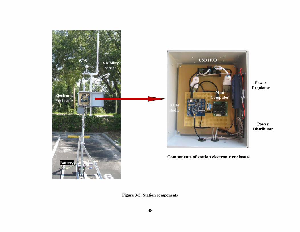
48

Components of station electronic enclosure

Figure 3-3: Station components

GPS Visibility sensor

Electronic Enclosure

Battery

USB HUB

XBee Radio

Mini Computer

Power Regulator

Power Distributor

Radio

A

USB HUB

49

3.2 Communications

Communication is the important part of the system; the system includes two types of

communication links. First, the internal communication link (data from sensors and base station)

is a 900 MHz radio. The second type is cellular communication which is used to exchange

information from the base station to the TMC. Any system is useless if it cannot report real-time

visibility conditions for warning drivers and TMC about reduced visibility conditions. For this

reason, the selection of a reliable communication system is of utmost importance. Thus, to avoid

typical line of sight limitations inherent in communication technologies such as WiFi, the spread

spectrum, etc., researches at UCF proposed the use of cell-based communication. This

communication mode guarantees national coverage and reduces hardware costs. Also, since this

system is designed to report on exceptional bases, data costs should be minimal.

3.3 System Operation

The visibility system is designed to be autonomous in its operation and decision-making.

It continuously monitors visibility. Whenever hazardous conditions are detected, it automatically

generates warning messages that can be displayed to motorists. Two types of messages are

generated; speed advisories and warning messages of poor visibility. The automatic messages are

selected by a computer algorithms based on the measured visibility distance and the maximum

safe speed.

50

3.4 Software Design and Algorithms

The system’s software control runs on a micro controller attached to the base station and

executes a real-time operating structure. The system controls the entire baseline functions

necessary to operate the overall system, including data acquisition, data storage, system control,

and self monitoring. Specifically, the system reads from 4 fog sensors, while controlling up to

four CMSs. This overall functionality is obtained through individual software modules, which

are illustrated in the diagram shown in Figure 3-4. The design of the system is extendible to

include additional fog sensors, VSL signs, flashing lights and DMSs to expand the capability of

the system to cover longer segments of roads in fog prone areas.

There are two main algorithms that have been designed to control the communications

process and data reporting frequencies. One of these algorithms controls the communications

between the stations and the base, while the other controls the communication between the base

and both CMSs and TMC.

As mentioned earlier, each station detects the visibility distance and reports it to the base

station. At normal conditions (highway visibility distance > 250 m), the base station receives

messages from each station showing the current visibility distance every 15 minutes. Although it

is not needed to take any action at normal visibility conditions, it was decided to receive

messages from each station to make sure that all stations are working properly. However, once

the visibility distance drops below hazardous visibility levels (<250 m), the reporting frequency

reduces to 1 minute.

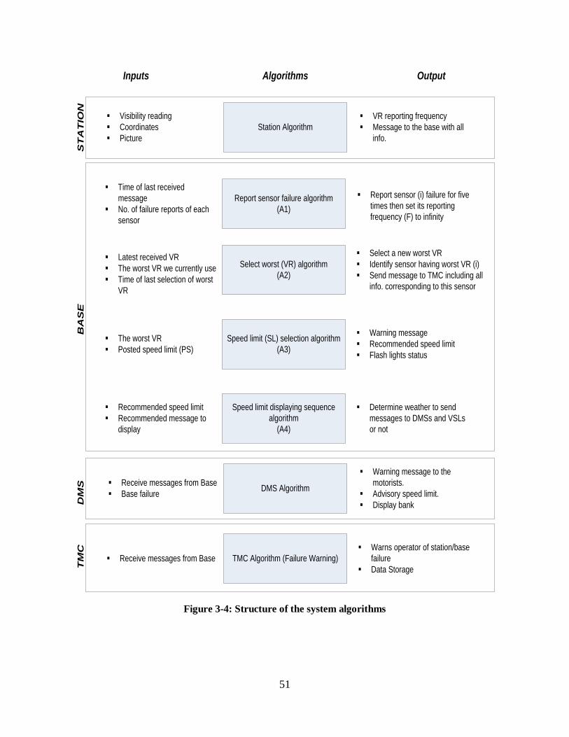
51

Figure 3-4: Structure of the system algorithms

OutputInputs AlgorithmsT

MC

TMC Algorithm (Failure Warning)§ Receive messages from Base§ Warns operator of station/base

failure§ Data Storage

DM

S DMS Algorithm§ Receive messages from Base§ Base failure

§ Warning message to the motorists.

§ Advisory speed limit.§ Display bank

Report sensor failure algorithm(A1)

§ Time of last received message

§ No. of failure reports of each sensor

§ Report sensor (i) failure for five times then set its reporting frequency (F) to infinity

Select worst (VR) algorithm(A2)

§ Latest received VR§ The worst VR we currently use§ Time of last selection of worst

VR

§ Select a new worst VR§ Identify sensor having worst VR (i)§ Send message to TMC including all

info. corresponding to this sensor

Speed limit (SL) selection algorithm(A3)

§ The worst VR§ Posted speed limit (PS)

§ Warning message§ Recommended speed limit§ Flash lights status

Speed limit displaying sequence algorithm

(A4)

§ Recommended speed limit§ Recommended message to

display

§ Determine weather to send messages to DMSs and VSLs or not

BA

SE

Station Algorithm§ Visibility reading§ Coordinates§ Picture

§ VR reporting frequency§ Message to the base with all

info.

ST

AT

ION

52

3.5 Testing the Radios’ Range

The objectives of testing the radios’ range of the developed visibility detection and

warning system were to determine the maximum range between two successive radios (one at the

base and the other at the station) and to examine the possibility of using an intermediate radio

(hopping) to increase the range between the base and the stations’ radios. The testing of radios’

range was divided into two stages. The first stage was conducted in the lab to make sure that the

system components are working properly however; the second stage was conducted in the field

to examine the system performance in real life.

To test the system in the field, the station and the base were installed at the UCF campus.

To simplify the test, the base station was installed on a truck and powered using a generator. A

laptop was attached to the base to check the receiving messages from the station. During

movement with the base away from the station, the base was receiving messages until the

distance increased more than 0.6 mile. At that point the communication between the base and the

station was lost. After using an intermediate radio (hopping) between the base and the station,

the radios’ range increased to about 1.2 mile.

3.6 Testing the System’s Performance

This section presents the preliminary performance’s testing of this visibility system. The

base and station were installed as shown in Figure 3-2 and Figure 3-3, respectively. To check the

performance of the base algorithm, the base was powered first using a car battery. Since the

station was not powered yet, the base sent an e-mail to TMC showing that no messages were

received from station(s) yet. This initial e-mail implies that the base is working properly, and

53

either the station(s) was non-powered yet or has a technical problem. Once the station was

powered, a message with the current visibility distance was sent (e.g., normal visibility

condition) to the base station which submitted an e-mail to TMC titled “normal conditions” and

contains station’s number, position (latitude and longitude), time and date of message. To test the

performance of the system in poor visibility conditions, a cloth bag was put on the visibility

sensor (because no fog existed when conducting the test). Thus the visibility measurement

dropped to zero and the station sent this message to the base which reported TMC with an

emergency e-mail titled “emergency: no visibility”. These warning e-mails can enable the TMC

and/or FDOT to take the appropriate decisions at such adverse visibility conditions. Table 3-1

summarizes the titles of all e-mails that could be sent to TMC/FDOT at all visibility levels. Once

the cloth bag was removed away from the visibility sensor, the station reported normal visibility

condition to the base. However, according to the design of the base algorithm, 5 minutes later the

base informed the TMC about improving the visibility range. The same email messages or

modification could also be sent to the CMS. Moreover, to test the base algorithm when loosing

communication between base and station(s), the base station was moved away from the station.

When the communication was lost, the base is programmed to send an e-mail to TMC entitled

“Station # 11 failure report”. This e-mail is important as it helps TMC to identify which station

has a problem so a technician can be dispatched to fix this problem immediately. Later, after

installing an intermediate radio, the base started again to receive messages from the station.

Figure 3-5 show examples of warning’s e-mail messages sent to TMC.

54

Table 3-1: E-mail message titles and frequency of reporting messages to TMC

E-mail Title Highway Visibility Range 1 EMERGENCY: No Visibility < 20ft 2 URGENT: Extremely low Visibility < 200ft 3 WARNING: Moderate visibility If visibility is between 200-500 ft

4 WARNING: Fog or Smoke Conditions affecting visibility

If visibility is between 500-800 ft

5 NORMAL CONDITIONS Visibility greater than 800 ft Frequency of reporting to TMC

Every hour Normal conditions. Every 1 Minute in Emergency Every 5 minutes otherwise

a) Emergency e-mail b) Normal condition e-mail

c) No received messages’ e-mail d) Station(s) failure e-mail

Figure 3-5: Examples of warning’s E-mail messages sent to TMC

55

3.7 Conclusions

This chapter presents the design of a visibility detection and warning system that was

developed by researchers at UCF. A discussion of the system components and performance was

introduced. The preliminary testing of this visibility system indicates that it can detect any

reduction in visibility in a timely manner and respond accordingly in real-time to convey specific

warning messages either by reporting these messages to TMC/FDOT through e-mails or by

displaying a warning message and an advisory safe speed at each visibility level using CMS and

VSL signs, respectively. However, before reaching a final conclusion about the performance of

this visibility detection system, conducting another field study at real fog condition is still

needed.

56

CHAPTER 4. SURVEY DESIGN AND CONTENT

This chapter presents the design and administration of a survey-based study focusing on

understanding commuters’ response to different visibility conditions due to fog/smoke in Central

Florida. A total of 566 respondents participated in this study through three survey approaches;

handout, interactive, and online questionnaire. The evaluation of the quality and completeness of

data received from the three surveys approaches as well as recommendations for the

improvement of future survey design and response are presented in this chapter.

4.1 Survey Design

To achieve the objectives of this survey, different scenarios consisting of several

visibility levels, traffic conditions, warning messages and advice displayed on CMS and VSL

signs were designed using driving simulation software, L-3 Scenario Editor. There is no doubt

that it would have been better to use real pictures in this study. However, the scenario editor

software was used to develop those scenarios since it was not possible to find real pictures for all

the scenarios that were developed. Snapshots at different fog levels, traffic conditions, and based

on the two roadway types were prepared before designing the two survey forms. It is worth

mentioning that due to limited budget and the various scenarios that were investigated in the

present study, neither field studies nor driving simulator experiments were feasible. Examples of

information displayed on both CMS and VSL signs are shown in Figure 4-1.

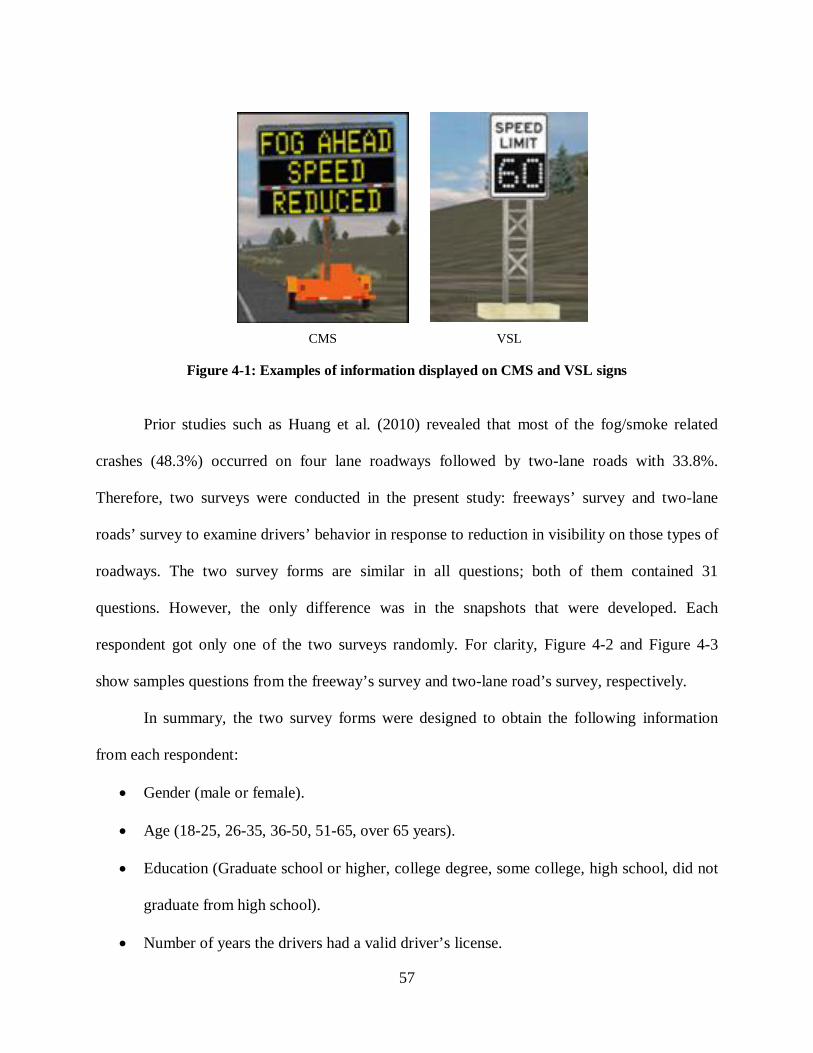
57

CMS VSL

Figure 4-1: Examples of information displayed on CMS and VSL signs

Prior studies such as Huang et al. (2010) revealed that most of the fog/smoke related

crashes (48.3%) occurred on four lane roadways followed by two-lane roads with 33.8%.

Therefore, two surveys were conducted in the present study: freeways’ survey and two-lane

roads’ survey to examine drivers’ behavior in response to reduction in visibility on those types of

roadways. The two survey forms are similar in all questions; both of them contained 31

questions. However, the only difference was in the snapshots that were developed. Each

respondent got only one of the two surveys randomly. For clarity, Figure 4-2 and Figure 4-3

show samples questions from the freeway’s survey and two-lane road’s survey, respectively.

In summary, the two survey forms were designed to obtain the following information

from each respondent:

• Gender (male or female).

• Age (18-25, 26-35, 36-50, 51-65, over 65 years).

• Education (Graduate school or higher, college degree, some college, high school, did not

graduate from high school).

• Number of years the drivers had a valid driver’s license.

58

• Number of traffic citations (i.e. traffic rule violations) in the previous 3 years.

• Involvement in any fog/smoke or heavy rain related crashes.

• Frequency of freeways/ two-lane roads use?

• Drivers’ familiarity with CMS and VSL signs.

• Drivers’ behavior when they encounter CMS at two traffic conditions (no car leading

ahead, and car leading ahead).

• Drivers’ behavior when they encounter a VSL sign at four fog conditions (very light fog,

light fog, medium fog, and heavy fog) and two traffic conditions (no car leading ahead,

and car leading ahead).

• Drivers’ satisfaction with the importance of CMS and VSL signs in providing

information that may help to manage the traffic flow along Highways and consequently

reducing the chances of a crash.

• Drivers’ satisfaction with using two successive CMS prior to Fog/ smoke zones.

• Which one of the following would improve safety during driving through fog/smoke

highways segments: using CMS only or using VSL signs only or using CMS and VSL

signs together or closing the road during such adverse weather conditions?

• What is the best CMS message that can be used to warn drivers about any reduction of

visibility due to fog/smoke and drivers will most likely comply with it.

• Drivers’ behavior when they encounter a sudden reduction in visibility due to fog, smoke,

or heavy rain while they are driving on a freeway/ two lane roads.

• Drivers’ ranking for the actions/responses that they can do when they encounter a sudden

reduction in visibility due to fog, smoke, or heavy rain while they are driving on a

freeway/ two lane roads.

59

If you were driving on a freeway with a speed limit of 65 mile/hour (mph), and you encounter a Variable Speed Limit (VSL) sign of 40 mile/hour (mph) in order to reduce the chances of accident that may occur because of a sudden reduction in visibility due to fog/smoke. What will you do in each of the following cases? Note: in case you will reduce your speed (answers c or d), please specify your reduced speed

Heavy Fog (some vehicles ahead) a) Do nothing b) Follow other vehicles’ speed. c) Reduce speed to ………..mph (Please specify your reduced speed) d) Put blinkers on and reduce speed to.…..mph

(Please specify your reduced speed)

Figure 4-2: Sample question from the freeway’s survey

If you were driving on a two lane road with a speed limit of 45 mile/hour (mph), and you encounter a Variable Speed Limit (VSL) sign of 25 mile/hour (mph) in order to reduce the chances of accident that may occur because of a sudden reduction in visibility due to fog/smoke. What will you do in each of the following cases? Note: in case you will reduce your speed (answers c or d), please specify your reduced speed

Heavy Fog (some vehicles ahead) a) Do nothing b) Follow other vehicles’ speed. c) Reduce speed to ………..mph (Please specify your reduced speed)

d) Put blinkers on and reduce speed to.…..mph (Please specify your reduced speed)

Figure 4-3: Sample question from the two lane road’s survey

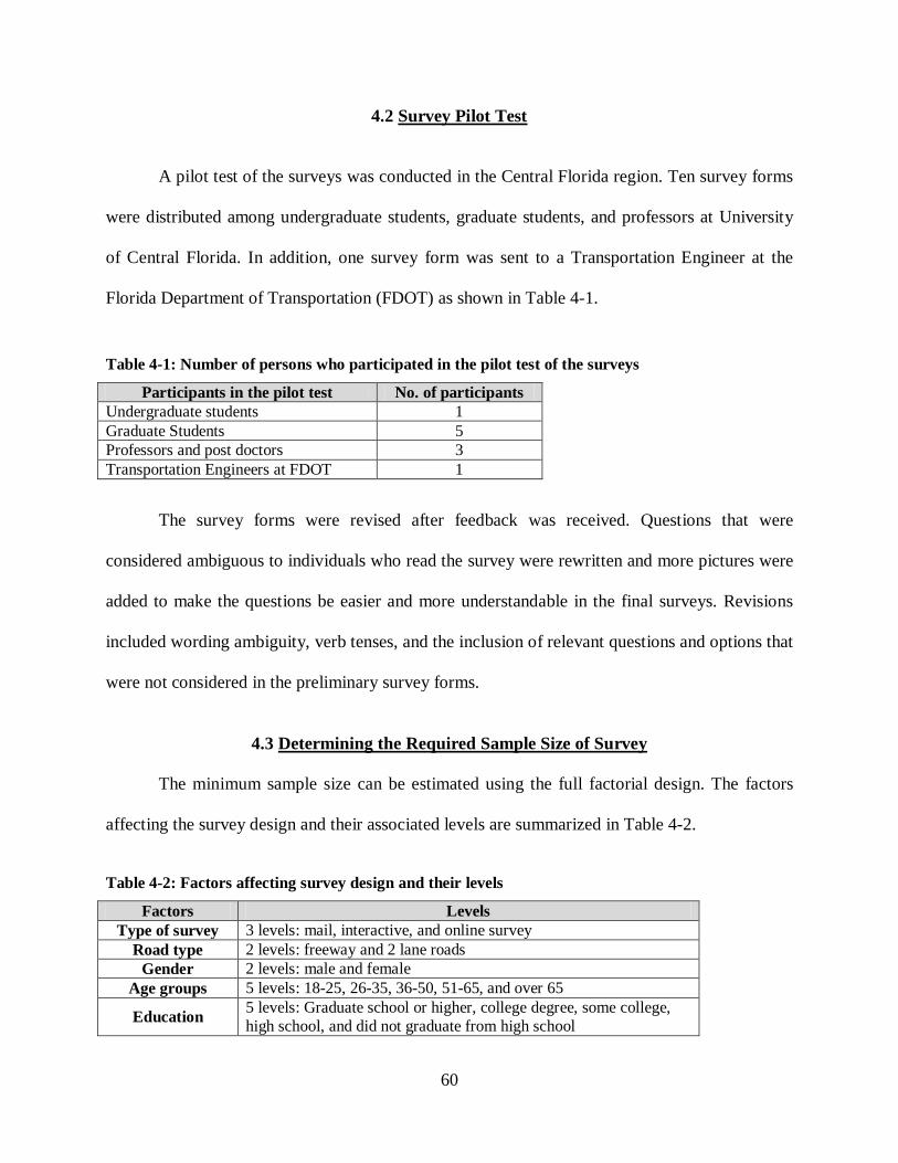
60

4.2 Survey Pilot Test

A pilot test of the surveys was conducted in the Central Florida region. Ten survey forms

were distributed among undergraduate students, graduate students, and professors at University

of Central Florida. In addition, one survey form was sent to a Transportation Engineer at the

Florida Department of Transportation (FDOT) as shown in Table 4-1.

Table 4-1: Number of persons who participated in the pilot test of the surveys

Participants in the pilot test No. of participants Undergraduate students 1 Graduate Students 5 Professors and post doctors 3 Transportation Engineers at FDOT 1

The survey forms were revised after feedback was received. Questions that were

considered ambiguous to individuals who read the survey were rewritten and more pictures were

added to make the questions be easier and more understandable in the final surveys. Revisions

included wording ambiguity, verb tenses, and the inclusion of relevant questions and options that

were not considered in the preliminary survey forms.

4.3 Determining the Required Sample Size of Survey

The minimum sample size can be estimated using the full factorial design. The factors

affecting the survey design and their associated levels are summarized in Table 4-2.

Table 4-2: Factors affecting survey design and their levels

Factors Levels Type of survey 3 levels: mail, interactive, and online survey

Road type 2 levels: freeway and 2 lane roads Gender 2 levels: male and female

Age groups 5 levels: 18-25, 26-35, 36-50, 51-65, and over 65

Education 5 levels: Graduate school or higher, college degree, some college, high school, and did not graduate from high school

61

Therefore, the minimum survey size = 3*2*2*5*5 = 300

To be more conservative, we recruited more than 500 participants in the survey as indicated in

the following sections.

4.4 Sampling Procedure and Survey Methods

The survey targeted a random sample of licensed drivers living in Orange and Seminole

counties. Respondents were limited to adults over 18 years of age who have a valid driver’s

license. Based on the review of previous studies, it was found that mail-in questionnaires yield

low response rates, and do not provide interaction between the interviewer and the respondent.

Hence, mail-in questionnaire was not undertaken. Also, phone interviews were not used because

of the need to incorporate images in the survey questions.

According to TCRP (2006), the use of Internet-based survey only usually does not

provide a representative sample of the population due to some population segments not having

access to the Internet or not having good knowledge about using the Internet. Thus, it was

decided to implement a 3-way approach to conduct the survey for both freeways and 2-lane

roads. The three survey types incorporated were handout, interactive, and online questionnaires.

4.4.1 Handout Questionnaire

The first survey approach was handout questionnaires. In this approach, 300 survey forms

were printed for each roadway type. These survey forms were distributed randomly in November

2009 among colleagues, friends, family, neighbors, faculty and staff who live in Central Florida.

Each one of them has received from 5 to 20 survey forms and he/she was asked to distribute

62

them among his/her colleagues, friends, neighbors and family members. They were asked to

return them once they are completed.

Out of the 600 distributed survey forms, a total of 376 forms were received back (62.7%

response rate). However, only 279 handout surveys’ forms were considered complete, 74%

complete responses (questions completed). The remaining forms had more than 30% missing

responses (questions) and hence, they were disregarded. Based on the respondents’ feedback, the

questionnaire took on average 10 minutes to be completed. It is worth mentioning that handout

surveys are better than the regular mail-back surveys due to the presence of personal interaction

between the surveyor and respondents.

4.4.2 Interactive Questionnaire

The second survey method was an interactive questionnaire. In this survey method, the

surveyor meets with a group of people at the same time and location and explains the purpose of

the survey and the steps they should follow to complete the questionnaire. In the current study,

the interactive survey was presented to two undergraduate classes and one graduate class at the

University of Central Florida in November 2009. Two presentations were designed for the two

survey forms in power point format. Each session gets either the freeway or 2-lane version. After

distributing the questionnaires to the respondents, each question or picture was presented in a full

screen using a projector. Participants were responding while the surveyor was explaining what is

meant by each question and interacting with them. Also, participants were allowed to ask

questions. The presentation and interaction was carefully considered so that the questions are

clarified but not to bias the responses. Each interactive questionnaire session lasted on average

20 minutes. The interactive survey sample contained 102 participants. However, only 91 forms

63

were used in the analysis, 89% complete responses (questions completed). Again the remaining

forms had more than 30% missing responses and thus they were disregarded.

4.4.3 Online Questionnaire

Online surveys have become more widespread in recent years. The advantages of

adopting online questionnaires include the possibility of sending a participation request to

randomly selected subjects using e-mail addresses. Second, respondents’ responses are

automatically saved in a database existing in the survey’s server, and can be retrieved at a later

time for data analysis. This simplifies the data processing for the analyst, eliminates coding

errors and reduces labor costs. Therefore, online questionnaires are less time consuming and less

labor-intensive than the other survey methods. Third, the use of graphical user interface (GUI)

and images provide the ability to better understand the questionnaire aspects (Abdel-Aty and

Abdelwahab, 2001; Peeta and Ramos, 2006). On the other hand, the limitations of online surveys

include the need accessibility of Internet and some knowledge of using the Internet by the

participants.

In this study, links for either survey type (freeway or 2-lane road) were sent randomly to

about 200 commuters in the Central Florida region in November 2009. Participants were asked

to estimate how many minutes they took to complete the survey and report it to the surveyor.

Also, 500 cards containing links to either survey forms were distributed randomly to drivers in

Central Florida.

At the beginning of each survey form, an introduction was provided explaining the

purpose of the survey and some guidelines for completing the survey. The advantages of the

present online survey include a warning pop-up appearing above any unanswered question

64

asking the respondents that this is required (as shown in Figure 4-4). This option might help to

increase the percent of complete responses in the online survey. The second advantage is that

respondents cannot enter the same answer for two or more options in question 31 (as shown in

Figure 4-5). Out of 231 received responses (33% response rate), 196 complete responses were

used in the analysis, 85% complete responses (questions completed), as the remaining forms had

more than 30% missing responses. Based on respondents’ feedback, the online questionnaire

took on average 8 minutes to be completed.

Figure 4-4: A warning hint about unanswered question in the online survey

65

Figure 4-5: A warning hint about entering the same ranking for two options in question 31 in the online survey

4.4.4 Validating Survey Sample

To test whether the sample well represents the licensed drivers in Orange and Seminole

counties, the percentages of gender and age groups of the survey sample were compared to the

corresponding percents of the licensed drivers in Orange and Seminole counties (January 2009)

that were obtained from the Florida Department of Highway Safety and Motor Vehicles

(DHSMV). Distributions of gender and age groups for the survey sample and licensed drivers in

Orange and Seminole counties in January 2009 are given in Table 4-3 and Table 4-4,

respectively.

66

Table 4-3: Distribution of gender for the survey sample and licensed drivers in Orange and Seminole counties

Gender Survey Licensed Drivers in Orange and Seminole counties (January, 2009)

Sample % Pop. % Male 310 54.8 615735 50.4

Female 256 45.2 606070 49.6 Total 566 100 1221805 100

Table 4-4: Distribution of age groups for the survey sample and licensed drivers in Orange and Seminole counties

Age Groups Survey Licensed Drivers in Orange and Seminole counties (January, 2009)

Sample % Pop. % 18-25 173 30.6 191925 16.1 26-35 120 21.2 255735 21.5 36-50 136 24.0 369507 31.0 51-65 98 17.3 243635 20.5

Over 65 39 6.9 130335 10.9 Total 566 100 1191135 100

To achieve this objective, Chi-Square test for specified proportions and a large-sample

test of hypothesis about a population proportion (Z-test) were developed as follows:

4.4.4.1 Chi-Square test for specified proportion

Hypothesis testing 1

H0: P1 = 0.504, P2 = 0.496 (the observed proportions of males and females in the survey sample

are not significantly different from the corresponding proportions of licensed drivers in

Orange and Seminole counties).

Ha: at least one of the multinomial probabilities does not equal its hypothesis.

Test Statistic

Chi-Square = 4.3244, DF=1, P-value=0.0876 > 0.05

67

Therefore, it can be concluded that the observed proportions of males and females in the survey

sample are not significantly different from the proportions of licensed male and female drivers in

Orange and Seminole counties

Hypothesis testing 2

H0: P1 = 0.161, P2 = 0.215, P3 = 0.310, P4 = 0.205, P5 = 0.109 (the observed proportions of age

groups in the survey sample are not significantly different from the corresponding

proportions of licensed drivers in Orange and Seminole counties).

Ha: at least one of the multinomial probabilities does not equal its hypothesis

Test Statistic

Chi-Square = 93.6088, DF=4, P-value=0.0001 < 0.05 then null hypothesis can be rejected.

Therefore, it can be concluded that at least one of the observed proportions of age groups in the

survey sample is significantly different from the corresponding proportions of licensed drivers in

Orange and Seminole counties. To investigate which age group has this difference, Z test was

developed.

4.4.4.2 Z- Test

Hypothesis testing

H0: P = P0 (the proportion of every age group in the survey sample is not significantly different

from the corresponding proportion of licensed drivers in Orange and Seminole counties).

Ha: P ≠ P0 (the proportion of every age group in the survey sample is significantly different from

the corresponding proportion of licensed drivers in Orange and Seminole counties).

68

Test Statistic

It can be realized that the percent of age group 18-25 (30.6%) is over-represented in the

survey sample because a large percent of the sample were students at UCF. However, in general

we can say that there are no significant differences between the age groups percents in the survey

sample and in the licensed drivers in Orange and Seminole counties.

In summary, considering the above mentioned results, it was concluded that there is no

significant difference between the percentages of males, females, age groups in the survey

sample and licensed drivers in Orange and Seminole counties. Hence, it was concluded that the

survey sample well represented the licensed drivers in Orange and Seminole counties.

4.5 Response Analysis

A total of 566 responses were used in this study. About 49.3% of these responses were

from handout survey, 16% through the interactive survey, and 34.7% via the Internet. As

mentioned earlier, the online survey has the shortest average time needed to be completed,

69

followed by handout, then interactive survey; 8, 10, and 20 minutes, respectively. Also, the

interactive survey has the highest percent of complete responses (questions completed) with

89%, followed by online survey with 85%, and followed by handout questionnaire with 74%,

respectively. Designing the online survey in a graphical user interface manner could be the

reason why it had the shortest average time and the second highest percent of complete responses

after the interactive survey. Also, in the interactive survey; surveyors had a direct interaction

with the participants to explain any ambiguousness they may find and this could explain why it

took the longest time.

The advantages and limitations of the three survey methods used in this study are

summarized in Table 4-5. According to Table 4-5, it can be concluded that the interactive survey

approach is recommended in future studies since it has high response rate, high control of

interview situation, high percent collection of detailed information, and the highest percent of

complete responses. This result is consistent with Nachimas (1996). On the other hand, the

disadvantages include that it has the longest time needed to complete the survey and it is difficult

to identify respondents. Therefore, the second recommended survey type is the online survey.

Table 4-5: Comparison between survey methods used in the current study

Criterion

Current study

Handout Interactive (controlled

group)

Online (web-based)

Cost Low Moderate Low Response rate Low High Moderate Control of interview situation Low High Moderate Collection of detailed information Moderate High High Speed of collecting survey forms Low Moderate High Average time to complete the survey forms (in minutes) 10 20 8

Percent of complete responses (questions completed) 74% 89% 85%

70

To investigate the differences between handout, interactive and online questionnaires,

conditional distribution, odds ratio, Chi-squared test, and Ridit analyses were developed. The

results of conditional distributions and odds ratios are listed in Table 4-6.

The odds ratios were estimated for each group with respect to the last category of that

group. Concerning the gender, the odds ratio of males equals 1.52, which implies that the odds

(or likelihood) of responding through the online survey are 1.5 times higher for males than for

females. Also regarding age, for example, the odds ratio of the age group 18-25 equals 2.7,

which means that the odds of responding via the Internet is 2.7 times higher for the age group of

16-25 than for the over 65 years old age group. This result supports the hypothesis that young

respondents are more likely to respond to the online survey than old participants.

With respect to the education levels, it was found that the odds ratio of education level

“graduate school or higher” equals 4.04, which indicates that the odds of responding through the

online survey are 4 times greater for this specific level than for respondents who did not graduate

from high schools. This finding supports the idea that Internet users might have a higher level of

education and awareness and therefore, are keen to respond in questionnaires related to studies

that are of interest. In this regards, the results shown in Table 4-6 indicate that the majority of

Internet respondents (87.75%) have some college degree or higher. In addition, Table 4-6

revealed that the majority of the Internet respondents (85.2%) are younger than 51 years old.

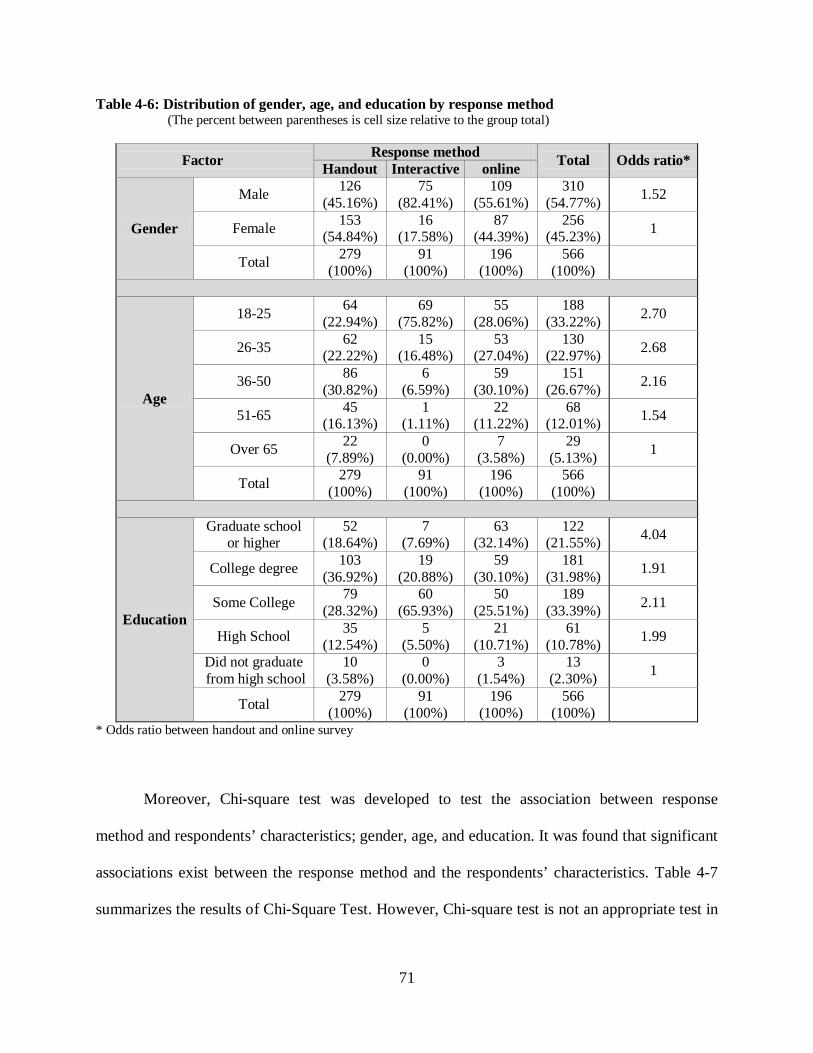
71

Table 4-6: Distribution of gender, age, and education by response method (The percent between parentheses is cell size relative to the group total)

Factor Response method Total Odds ratio* Handout Interactive online

Gender

Male 126 (45.16%)

75 (82.41%)

109 (55.61%)

310 (54.77%) 1.52

Female 153 (54.84%)

16 (17.58%)

87 (44.39%)

256 (45.23%) 1

Total 279 (100%)

91 (100%)

196 (100%)

566 (100%)

Age

18-25 64 (22.94%)

69 (75.82%)

55 (28.06%)

188 (33.22%) 2.70

26-35 62 (22.22%)

15 (16.48%)

53 (27.04%)

130 (22.97%) 2.68

36-50 86 (30.82%)

6 (6.59%)

59 (30.10%)

151 (26.67%) 2.16

51-65 45 (16.13%)

1 (1.11%)

22 (11.22%)

68 (12.01%) 1.54

Over 65 22 (7.89%)

0 (0.00%)

7 (3.58%)

29 (5.13%) 1

Total 279 (100%)

91 (100%)

196 (100%)

566 (100%)

Education

Graduate school or higher

52 (18.64%)

7 (7.69%)

63 (32.14%)

122 (21.55%) 4.04

College degree 103 (36.92%)

19 (20.88%)

59 (30.10%)

181 (31.98%) 1.91

Some College 79 (28.32%)

60 (65.93%)

50 (25.51%)

189 (33.39%) 2.11

High School 35 (12.54%)

5 (5.50%)

21 (10.71%)

61 (10.78%) 1.99

Did not graduate from high school

10 (3.58%)

0 (0.00%)

3 (1.54%)

13 (2.30%) 1

Total 279 (100%)

91 (100%)

196 (100%)

566 (100%)

* Odds ratio between handout and online survey

Moreover, Chi-square test was developed to test the association between response

method and respondents’ characteristics; gender, age, and education. It was found that significant

associations exist between the response method and the respondents’ characteristics. Table 4-7

summarizes the results of Chi-Square Test. However, Chi-square test is not an appropriate test in

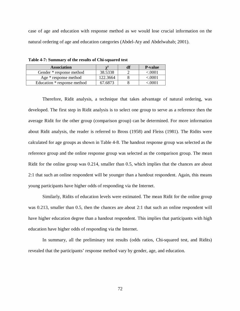
72

case of age and education with response method as we would lose crucial information on the

natural ordering of age and education categories (Abdel-Aty and Abdelwahab; 2001).

Table 4-7: Summary of the results of Chi-squared test

Association χ² df P-value Gender * response method 38.5338 2 <.0001

Age * response method 122.3664 8 <.0001 Education * response method 67.6873 8 <.0001

Therefore, Ridit analysis, a technique that takes advantage of natural ordering, was

developed. The first step in Ridit analysis is to select one group to serve as a reference then the

average Ridit for the other group (comparison group) can be determined. For more information

about Ridit analysis, the reader is referred to Bross (1958) and Fleiss (1981). The Ridits were

calculated for age groups as shown in Table 4-8. The handout response group was selected as the

reference group and the online response group was selected as the comparison group. The mean

Ridit for the online group was 0.214, smaller than 0.5, which implies that the chances are about

2:1 that such an online respondent will be younger than a handout respondent. Again, this means

young participants have higher odds of responding via the Internet.

Similarly, Ridits of education levels were estimated. The mean Ridit for the online group

was 0.213, smaller than 0.5, then the chances are about 2:1 that such an online respondent will

have higher education degree than a handout respondent. This implies that participants with high

education have higher odds of responding via the Internet.

In summary, all the preliminary test results (odds ratios, Chi-squared test, and Ridits)

revealed that the participants’ response method vary by gender, age, and education.

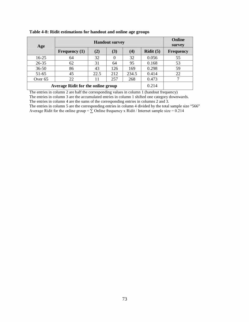
73

Table 4-8: Ridit estimations for handout and online age groups

Age Handout survey Online

survey Frequency (1) (2) (3) (4) Ridit (5) Frequency

16-25 64 32 0 32 0.056 55 26-35 62 31 64 95 0.168 53 36-50 86 43 126 169 0.298 59 51-65 45 22.5 212 234.5 0.414 22

Over 65 22 11 257 268 0.473 7 Average Ridit for the online group 0.214

The entries in column 2 are half the corresponding values in column 1 (handout frequency) The entries in column 3 are the accumulated entries in column 1 shifted one category downwards. The entries in column 4 are the sums of the corresponding entries in columns 2 and 3. The entries in column 5 are the corresponding entries in column 4 divided by the total sample size “566” Average Ridit for the online group = ∑ Online frequency x Ridit / Internet sample size = 0.214

74

4.6 Conclusions Regarding Survey Methods

This chapter presents the design and administration of a survey-based study to explore

commuters’ responses to different visibility conditions due to fog/smoke. The survey consisted

of 566 responses through three different survey approaches; handout, interactive, and online

questionnaires. Discussion of the quality and completeness of responses received by these three

approaches were presented. Also, the advantages and limitations of the three survey methods

used in this study were presented and discussed.

The results indicated that the online survey has the shortest average time needed to be

completed, followed by handout, then interactive survey; 8, 10, and 20 minutes, respectively.

Also, the interactive survey has the highest percent of complete responses (questions completed)

with 89%, followed by online survey with 85%, and followed by handout questionnaire with

74%, respectively. Designing the online survey in a graphical user interface manner could be the

reason why it had the shortest average time and the second highest percent of complete responses

after the interactive survey. Also, in the interactive survey; surveyors have a direct interaction

with the participants to explain any ambiguousness they may find and this could explain why it

took the longest time. Moreover, concerning the quality and completeness of responses, it was

found that the handout survey is even better than regular mail-back survey as personal interaction

exists between the surveyors and respondents in the handout questionnaire case.

In addition, several categorical data analysis techniques were applied to understand the

difference between handout, interactive, and online responses. These methods include odds ratio,

Chi-squared test, and Ridits analysis.

The results depict that the odds of online responses are much higher for young

respondents (18-25 years old). This implies that young respondents are more likely to respond to

75

the online survey than older participants possibly because young respondents are more used to

using the Internet than older participants. These results are consistent with the result obtained by

Abdel-Aty and Abdelwahab (2001). Also, compared to participants who just have a high school

degree or less, the findings revealed that online respondents might have a higher level of

education and awareness and therefore, are keen to respond to questionnaires related to studies

that could affect and benefit them. In this regards, it was found that the majority of Internet

respondents (87.75%) have some college degree or higher.

It can be concluded that the interactive survey approach is recommended in future studies

since it has high response rate, high control of interview situation, high percent collection of

detailed information, and the highest percent of complete responses. On the other hand, the

disadvantages include that it has the longest time needed to complete the survey and it is difficult

to identify respondents. Therefore, when conducting an interactive survey is not possible, the

second recommended survey type is the online survey as it has the shortest time to be completed

and the second highest percentage of complete responses (questions completed) after the

interactive survey. Also, conducting the survey with a combination of survey methods such as

handout or phone is highly recommended to obtain a well representative survey sample.

76

CHAPTER 5. SURVEY ANALYSIS

5.1 Description of the Survey Sample

As indicated earlier, a total of 566 responses were used in the analysis presented in this

survey study. The frequencies and percentages of the survey sample are summarized in Table 5-

1. As shown in Table 5-1, about 54.8% and 45.2% of participants were males and females,

respectively. Also, about 49.3% of responses were from the handout survey, 16% through the

interactive survey, and 34.7% via the Internet. Moreover, the number of respondents for the

freeway and the two-lane road surveys were 262 (46.3%) and 304 (53.7%), respectively.

Respondents were asked if they were involved in previous crashes due to FS or HR.

According to Table 5-1, about 3.9% and 10.8% of the respondents reported that were involved in

FS and HR-related crashes, respectively.

5.2 Response Analysis

Respondents were asked if they have encountered CMS and VSL signs on freeways/two

lane roads. The results indicated that the majority of respondents (83.6% and 68.2%) are familiar

with CMS and VSL signs, respectively.

As mentioned earlier, one of the objectives of this study is to determine the content of the

message that is perceived to achieve the best safety and achieve drivers’ compliance.

Considering drivers’ opinions, 216 respondents (38%) stated that the best message is “Caution-

fog ahead-reduce speed”. By testing the homogeneity of proportions of the given messages, the

hypothesis that all proportions are equal was rejected at the 5% level of significance (χ2=274.7,

77

DF=5, p-value<0.0001) which implies that there is significant difference in selection of

messages and that the aforementioned message was selected as the best message by the larger

proportion of participants. The percentages of drivers’ choices for other alternative messages are

listed in Table 5-1.

In addition, the responses revealed that the majority of respondents (83.2%) agree with

the usefulness of using two successive CMS prior to FS zones for warning drivers about any

sudden reduction in visibility. This could provide drivers with another chance to read the content

of the warning message of the second CMS if they missed the first one.

Furthermore, drivers were asked about their satisfaction with the usefulness of using

CMS and VSL signs on a five-point scale ranging from “strongly disagree” to “strongly agree”.

About 93.5% of respondents (who agree or strongly agree) reported that they are satisfied with

the usefulness of CMS while, 76% of participants (who agree or strongly agree) stated that VSL

signs could be useful in reducing the number of FS crashes (as shown in Table 5-1). This

difference could be attributed to the fact that drivers in Florida are not familiar with VSL signs

compared to CMS.

Another objective of this study was to investigate the best way to improve safety during

driving through FS zones based on drivers’ expectations and preferences: using CMS only, using

VSL signs only, using CMS and VSL signs simultaneously or closing the road during such

adverse weather. Most of the respondents (63.8%) stated that using CMS and VSL signs together

is the best way to improve safety during reduced visibility conditions (as shown in Table 5-1).

78

Table 5-1: Survey sample distributions

Variables Categories Number of Respondents

Percentages of Respondents

Gender Male 310 54.8 Female 256 45.2

Age Groups

18-25 173 30.6 26-35 120 21.2 36-50 136 24.0 +51 137 24.2

Education Levels

Graduate school or higher 122 21.6 College degree 182 32.1 Some College 188 33.2 High School or less 74 13.1

Survey type Handout 279 49.3 interactive 91 16.0 online 196 34.7

Road type Freeways 262 46.3 two lane roads 304 53.7

Involved in FS crashes yes 22 3.9 no 544 96.1

Involved in HR crashes yes 61 10.8 no 505 89.2

Drivers’ familiarity with CMS yes 473 83.6 no 93 16.4

Drivers’ familiarity with VSL signs

yes 386 68.2 no 180 31.8

Drivers' opinion of the messages that will achieve the best safety and driver compliance

Fog ahead-Reduce speed 71 12.5 Caution-Fog ahead-reduce speed 216 38.2 Fog ahead-Reduce speed-fine doubled 91 16.1 Fog ahead- Reduce speed –Strictly enforced 132 23.3

Caution- Reduce speed –Strictly enforced 41 7.2 Other 15 2.7

Drivers' opinion about the best way to improve safety during poor visibility conditions

using CMS only 176 31.1 using VSL only 16 2.8 using CMS and VSL together 361 63.8 close the road 13 2.3

Drivers’ satisfaction with the usefulness of CMS in warning them about reduced visibility conditions

Strongly agree 268 47.4 Agree 261 46.1 Neither agree nor disagree 24 4.2 Disagree 13 2.3 Strongly disagree 0 0

Drivers’ satisfaction with the usefulness of VSL in reducing the number of fog related crashes by informing them about safe speed limit under reduced visibility conditions

Strongly agree 187 33.0 Agree 243 42.9 Neither agree nor disagree 78 13.8 Disagree 47 8.4

Strongly disagree 11 1.9

79

This result is logical because warning drivers that there is fog ahead using CMS only

does not instruct them on what to do. Therefore, using VSL signs is also important to advise

drivers about the safe speed at every visibility conditions. This result is consistent with prior

studies such as Perrin et al. (2002). The hypothesis that the proportions of all possible ways to

improve safety are equal was rejected at the 5% level of significance (χ2=576.9, DF=3, p-

value<0.0001) which means that using CMS and VSL signs together during adverse visibility

conditions was preferred by the larger proportion of participants.

To obtain an in-depth understanding of drivers’ behavior in response to CMS and VSL

instructions at different visibility conditions, 10 scenarios were designed for both; freeways and

two-lane roads (as shown in Table 5-2). Two scenarios include two pictures for a freeway/a two-

lane road and a CMS displaying the following message: “Fog ahead – speed reduced” (As shown

in Figure 5-1). Respondents were asked about their possible actions when driving on a freeway at

a speed of 65 mph (or on a two-lane road at a speed of 45 mph), and they encountered a portable

CMS advising them to reduce speed due to reduction in visibility at two conditions: low traffic

volumes (no car leading ahead) and medium-high traffic volumes (some vehicles are ahead).

Table 5-2: Description of scenarios

Scenario Sign Visibility conditions Traffic conditions

1 CMS Light fog No car leading ahead 2 Some vehicles are ahead 3

VSL

Very light fog

No car leading ahead 4 Light fog 5 Medium fog 6 Heavy fog 7 Very light fog

Some vehicles are ahead 8 Light fog 9 Medium fog 10 Heavy fog

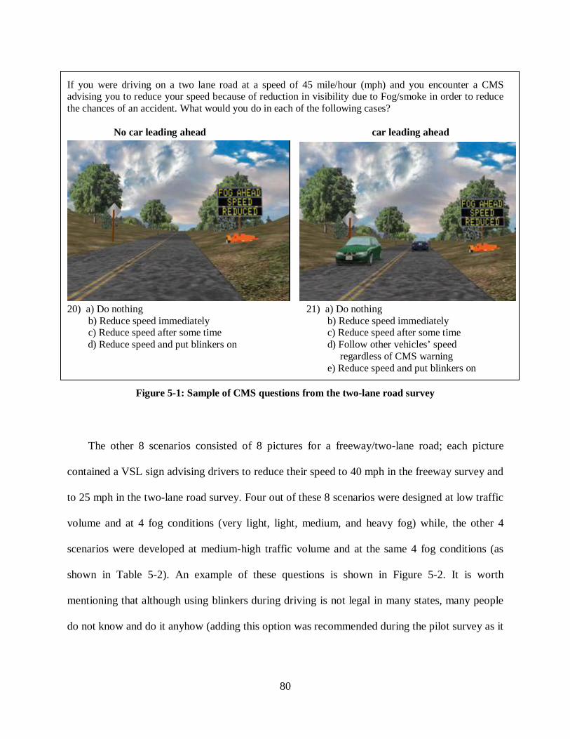
80

If you were driving on a two lane road at a speed of 45 mile/hour (mph) and you encounter a CMS advising you to reduce your speed because of reduction in visibility due to Fog/smoke in order to reduce the chances of an accident. What would you do in each of the following cases? No car leading ahead car leading ahead

20) a) Do nothing 21) a) Do nothing b) Reduce speed immediately b) Reduce speed immediately c) Reduce speed after some time c) Reduce speed after some time

d) Reduce speed and put blinkers on d) Follow other vehicles’ speed regardless of CMS warning e) Reduce speed and put blinkers on

Figure 5-1: Sample of CMS questions from the two-lane road survey

The other 8 scenarios consisted of 8 pictures for a freeway/two-lane road; each picture

contained a VSL sign advising drivers to reduce their speed to 40 mph in the freeway survey and

to 25 mph in the two-lane road survey. Four out of these 8 scenarios were designed at low traffic

volume and at 4 fog conditions (very light, light, medium, and heavy fog) while, the other 4

scenarios were developed at medium-high traffic volume and at the same 4 fog conditions (as

shown in Table 5-2). An example of these questions is shown in Figure 5-2. It is worth

mentioning that although using blinkers during driving is not legal in many states, many people

do not know and do it anyhow (adding this option was recommended during the pilot survey as it

81

is a common driving behavior . Also, it was decided to study drivers’ responses to CMS at only

one fog condition (light fog) to reduce the numbers of survey’s questions.

If you were driving on a freeway with a speed limit of 65 mile/hour (mph), and you encounter a Variable Speed Limit Sign of 40 mile/hour (mph) to reduce the chances of an accident that may occur because of a sudden reduction in visibility due to fog/smoke. What will you do in each of the following cases?

Note: in case you will reduce your speed (answers c or d), please specify your reduced speed a) Do nothing b) Follow other vehicles’ speed. c) Reduce speed to ………..mph (Please specify your reduced speed) d) Put blinkers on and reduce speed to…...mph (Please specify your reduced speed) Very Light Fog Light Fog

Medium Fog Heavy Fog

Figure 5-2: Sample of VSL questions from the freeway survey

Drivers’ responses to CMS and VSL signs at different fog and traffic conditions for both:

freeway and two-lane road cases are summarized in Table 5-3 and Table 5-4, respectively. Table

5-3 indicates that only 37% of the respondents reported that they would reduce speed

82

immediately or reduce speed and put blinkers on when encountered CMS, which advises them to

reduce speed due to reduced visibility condition, at low traffic volume while driving on a

freeway. At medium-high traffic volume, this percentage increased to 51.6%. This seems

reasonable because of the effect of traffic volume as it is one of the most important factors

affecting drivers’ behavior.

For two-lane road case, the percentages of drivers who were willing to reduce speed

immediately or reduce speed and put blinkers on following CMS instructions at low and

medium-high traffic volumes are 38.5% and 56.9%, respectively. Again, this result implies that

drivers are more cautious when driving at medium-high traffic volume. Although Table 5-3

indicates that drivers are more cautious when driving on two-lane roads at adverse visibility

conditions compared with driving on freeways. However, using Z-test, the differences of

proportions between drivers’ response when driving on freeways and on two-lane roads were not

statistically significant.

Table 5-3: Summary of drivers’ responses to CMS instructions

Traffic conditions

Fog conditions

Do nothing

Reduce speed after some

time

Follow other vehicles’ speed

Reduce speed immediately or

reduce speed and put blinkers on

Drivers’ behavior for Freeway Survey (Sample size = 262) Low traffic

volume Light fog

56 (21.4%) 109 (41.6%) NA* 97 (37%)

Medium –high traffic

volume 20 (7.6%) 63 (24%) 44 (16.8%) 135 (51.6%)

Drivers’ behavior for Two-Lane Road Survey (Sample size = 304) Low traffic

volume Light fog

44 (14.5%) 143 (47%) NA* 117 (38.5%)

Medium –high traffic

volume 11 (3.6%) 71 (23.4%) 49 (16.1%) 173 (56.9%)

* Not Applicable

83

As shown in Table 5-4, clearly both fog and traffic conditions greatly affect drivers’

responses to safe speed limits displayed on VSL signs at each of the aforementioned 8 scenarios.

As the visibility distance is reduced and traffic volume increases, drivers tend to follow VSL

instructions. With respect to the survey made in freeway, the percentage of respondents who

would reduce their speed or reduce speed and put blinkers on increased from 63.4 to 77.1 to 96.6

to 98.5% for low traffic volumes and increased from 44.7 to 51.1 to 76 to 89.7% for medium-

high traffic volumes. Higher values were obtained for the two-lane road’s survey. Again this

implies that traffic volume, type of road, and visibility condition affected the likelihood of

reducing the speed following VSL/CMS instructions.

Table 5-4: Summary of drivers’ responses to VSL sign instructions

Drivers’ behavior for Freeway Survey (Sample size = 262)

Traffic conditions

Fog conditions Do nothing

Follow other vehicles’

speed

Reduce speed or reduce speed and put blinkers on

Reduce speed to 40 MPH or less

Low traffic volume

Very light fog 96 (36.6%) NA* 166 (63.4%) 92 (35.1%) Light fog 60 (22.9%) NA* 202 (77.1%) 104 (39.7%)

Medium fog 9 (3.4%) NA* 253 (96.6%) 155 (59.2) Heavy fog 4 (1.5%) NA* 258 (98.5%) 201 (76.7%)

Medium–high traffic volume

Very light fog 43 (16.4%) 102 (38.9%) 117 (44.7%) 93 (35.5%) Light fog 22 (8.4%) 106 (40.5%) 134 (51.1%) 107 (40.8%)

Medium fog 4 (1.5%) 59 (22.5%) 199 (76.0) 159 (60.7%) Heavy fog 2 (0.8%) 25 (9.5%) 235 (89.7%) 215 (82.1%) Drivers’ behavior for Two-Lane Road Survey (Sample size = 304)

Traffic conditions

Fog conditions Do nothing

Follow other vehicles’

speed

Reduce speed or reduce speed and put blinkers on

Reduce speed to 25 MPH or less

Low traffic volume

Very light fog 110 (36.2%) NA* 194 (63.8%) 108 (35.5%) Light fog 65 (21.4%) NA* 239 (78.6%) 127 (41.8%)

Medium fog 8 (2.6%) NA* 296 (97.4%) 183 (60.2%) Heavy fog 2 (0.7%) NA* 302 (99.3%) 242 (79.6%)

Medium–high traffic volume

Very light fog 44 (14.5%) 113 (37.2%) 147 (48.3%) 117 (38.5%) Light fog 24 (7.9%) 121 (39.8%) 159 (52.3%) 141 (46.4%)

Medium fog 0 (0%) 64 (21.1%) 240 (78.9%) 196 (64.5%) Heavy fog 0 (0%) 25 (8.2%) 279 (91.8%) 262 (86.2%)

* Not Applicable

84

Furthermore, as shown in the last column of Table 5-4, only 35.1% of respondents stated

that they would follow VSL signs’ instructions (reduce their speed to 40 mph or less) while

driving on a freeway at very light fog and low traffic volume. The results also reveal that the

percentages of drivers who are willing to follow VSL instructions increase as the visibility

distance deteriorates and traffic volume increases. For example, the percentage increased to

82.1% at heavy fog and medium-high traffic volume. The same conclusion applies to two-lane

roads but with higher percentages of compliance with VSL instruction. However, using Z and

Chi Square tests, no significant differences were found between drivers’ responses to VSL signs

while driving on freeways versus two-lane roads or while driving at low versus medium-high

traffic volumes.

Finally drivers were asked to rank the following six options from the safest action (rank

1) that they thought would minimize the chance of a FS crash to the least action (rank 6): 1) do

nothing, 2) drive below speed limit, 3) drive below speed limit following the instructions of

CMS and VSL signs, if they are available, 4) follow other vehicles’ speed regardless of CMS and

VSL warnings, 5) drive below speed limit and put blinkers on, 6) Abandon the journey and stop

the car immediately at the right shoulder of the road.

The results revealed that 36.2% of the respondents claimed that following the instructions

of CMS and VSL signs is the safest action. Driving below speed limit and putting blinkers on

came in the second place with 26.3%. On the other hand, the majority of sample (86%) stated

that doing nothing is the most dangerous action. “Abandon the journey and stop the car

immediately at the right shoulder of the road” came next with about 10%. Some participants

pointed out that the last option is dangerous as it might increase rear-end crashes especially at

heavy fog condition.

85

5.3 Association between Categorical Variables

Prior to the modeling process, conditional distributions, odds’ ratios, and Chi square tests

were used for preliminary investigation of the differences between drivers’ responses to CMS

and VSL signs at different traffic and visibility conditions. Table 5-5 summarizes the results of

conditional distributions and odds ratios. The odds’ ratios were estimated for each group with

respect to the first category of that group.

As shown in Table 5-5, concerning the gender, the odds’ ratio of females equals 3.7,

which implies that when driving at heavy fog and medium-high traffic volume, the odds of

following VSL instructions are 3.7 times higher for females than males. Also regarding age, the

result supports the hypothesis that older respondents are more likely to respond to VSL

instructions than young participants. For example, the results revealed that the likelihood of

following VSL instructions is 5.1 times higher for old drivers than for young drivers (18-25 years

old).

Regarding drivers’ familiarity with VSL signs, it was found that the odds of following

VSL instructions are 2.6 times greater for drivers who are familiar with VSL than for those who

are not. In addition, the likelihood of following VSL instructions is 2.1 times higher for

experienced drivers than drivers who are not familiar with driving at poor visibility conditions.

Similar results were obtained for drivers’ response to CMS (see Table 5-5). Concerning road

type, it was found that the probability of following CMS while driving on two-lane roads is 1.2

times higher than while driving on freeways.

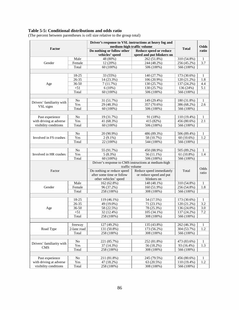
86

Table 5-5: Conditional distributions and odds ratio (The percent between parentheses is cell size relative to the group total)

Factor

Driver’s response to VSL instructions at heavy fog and medium-high traffic volume Total Odds

ratio Do nothing or follow other vehicles’ speed

Reduce speed or reduce speed and put blinkers on

Gender Male 48 (80%) 262 (51.8%) 310 (54.8%) 1

Female 12 (20%) 244 (48.2%) 256 (45.2%) 3.7 Total 60 (100%) 506 (100%) 566 (100%)

Age

18-25 33 (55%) 140 (27.7%) 173 (30.6%) 1 26-35 14 (23.3%) 106 (20.9%) 120 (21.2%) 1.8 36-50 7 (11.7%) 130 (25.7%) 137 (24.2%) 4.4 +51 6 (10%) 130 (25.7%) 136 (24%) 5.1

Total 60 (100%) 506 (100%) 566 (100%)

Drivers’ familiarity with VSL signs

No 31 (51.7%) 149 (29.4%) 180 (31.8%) 1 Yes 29 (48.3%) 357 (70.6%) 386 (68.2%) 2.6

Total 60 (100%) 506 (100%) 566 (100%)

Past experience with driving at adverse

visibility conditions

No 19 (31.7%) 91 (18%) 110 (19.4%) 1 Yes 41 (68.3%) 415 (82%) 456 (80.6%) 2.1

Total 60 (100%) 506 (100%) 566 (100%)

Involved in FS crashes No 20 (90.9%) 486 (89.3%) 506 (89.4%) 1 Yes 2 (9.1%) 58 (10.7%) 60 (10.6%) 1.2

Total 22 (100%) 544 (100%) 566 (100%)

Involved in HR crashes No 55 (91.7%) 450 (88.9%) 505 (89.2%) 1 Yes 5 (8.3%) 56 (11.1%) 61 (10.8%) 1.4

Total 60 (100%) 506 (100%) 566 (100%)

Factor

Driver’s response to CMS instructions at medium-high traffic volume

Total Odds ratio Do nothing or reduce speed

after some time or follow other vehicles’ speed

Reduce speed immediately or reduce speed and put

blinkers on

Gender Male 162 (62.8%) 148 (48.1%) 310 (54.8%) 1

Female 96 (37.2%) 160 (51.9%) 256 (54.8%) 1.8 Total 258 (100%) 308 (100%) 566 (100%)

Age

18-25 119 (46.1%) 54 (17.5%) 173 (30.6%) 1 26-35 49 (19.0%) 71 (23.1%) 120 (21.2%) 3.2 36-50 58 (22.5%) 78 (25.3%) 136 (24.0%) 3.0 +51 32 (12.4%) 105 (34.1%) 137 (24.2%) 7.2

Total 258 (100%) 308 (100%) 566 (100%)

Road Type freeway 127 (49.2%) 135 (43.8%) 262 (46.3%) 1

2-lane road 131 (50.8%) 173 (56.2%) 304 (53.7%) 1.2 Total 258 (100%) 308 (100%) 566 (100%)

Drivers’ familiarity with CMS

No 221 (85.7%) 252 (81.8%) 473 (83.6%) 1 Yes 37 (14.3%) 56 (18.2%) 93 (16.4%) 1.3

Total 258 (100%) 308 (100%) 566 (100%)

Past experience with driving at adverse

visibility conditions

No 211 (81.8%) 245 (79.5%) 456 (80.6%) 1 Yes 47 (18.2%) 63 (20.5%) 110 (19.4%) 1.2

Total 258 (100%) 308 (100%) 566 (100%)

87

Additionally, one more interesting research question was to examine whether drivers’

responses to reduced visibility conditions differed for those who were involved in FS or HR

crashes. As expected, it was found that when driving at heavy fog and medium-high traffic

volume, the odds of following VSL instructions is 1.2 times higher for participants who were

involved in FS crashes than those who were not involved in such crashes (as shown in Table 5-

5). Similarly, the odds of following VSL signs at heavy fog condition and medium-high traffic

volume is 1.4 times higher for participants who were previously experienced HR crashes than

those who were not involved in such crashes.

Moreover, Pearson Chi-Square test (χ2) and Mantel-Haenszel Chi-Square test (CMH)

were developed to explore the association between drivers’ responses to CMS/VSL signs and

other factors such as age, gender, education, drivers’ familiarity with CMS/VSL signs, and

experience with driving at adverse visibility conditions. Chi-Square test was used to test the

independence of every two nominal variables while, CMH test was used to examine the

association between every two ordinal variables or between ordinal and nominal variables.

The results showed significant association between drivers’ response to VSL/CMS signs

and those variables shown in Table 5-6.

88

Table 5-6: Summary of Pearson Chi-Squared and Mantel-Haenszel tests’ results

Factors Value DF P-value Factors associated with drivers’ responses to VSL instructions

at heavy fog and medium to high traffic volume (1) Gender χ2 =20.770 4 0.000 Age CMH =58.943 12 0.000 Education CMH =22.978 12 0.028 Drivers’ familiarity with VSLS χ2 =15.045 3 0.002 Past experience with driving at poor visibility condition χ2 =8.391 3 0.039

Factors associated with drivers’ responses to VSL instructions at very light fog and low traffic volume (2)

Gender χ2 =7.889 2 0.019 Age CMH =67.117 8 0.000

Factors associated with drivers’ responses to CMS instructions at low traffic volume (3)

Gender χ2 =12.127 3 0.007 Age CMH =94.622 12 0.000 Education CMH =43.128 12 0.000 Drivers’ familiarity with driving on freeway/2 lane road χ2 =9.693 3 0.021 Drivers’ familiarity with PCMS χ2 =8.668 3 0`.034

Factors associated with drivers’ responses to CMS instructions at medium to high traffic volume (4)

Gender χ2 =14.601 4 0.006 Age CMH =110.418 16 0.000 Education CMH =35.570 16 0.003 (1) * (2) χ2 =62.068 6 0.000 (1) * (3) χ2 =105.904 9 0.000 (1) * (4) χ2 =129.065 12 0.000 (2) * (3) χ2 =141.239 6 0.000 (2) * (4) χ2 =109.491 8 0.000 (3) * (4) χ2 =652.313 12 0.000

* Only significant associations are shown in the table

In summary, all the preliminary tests’ results revealed that the participants’ response to

CMS and VSL signs instructions vary by gender, age, familiarity with CMS and VSL signs, and

experience with driving at adverse visibility condition. Thus, to improve our understanding of

the preferences of respondents in following VSL and CMS instructions at such adverse visibility

conditions, multivariate analyses; the bivariate and multivariate probit models were employed for

further analyses.

89

5.4 Bivariate and Multivariate Probit Approach

This section emphasizes two methodological approaches for analyzing and modeling

drivers’ responses to CMS and VSL signs at different visibility and traffic conditions; Bivariate

Probit Models (BPM) and Multivariate Probit Model (MPM). Correlated responses often arise in

behavioral, medical and psychological researches. BPM and MPM are popular methods for

analyzing this kind of data (Lu and Song, 2006).

MPM has been widely used in agricultural, statistical, and economic studies for analyzing

potentially correlated multivariate outcomes. These studies include Gibbons and Wilcox (1998),

Lansink et al. (2003), and Young et al. (2009). However, MPM has been developed in few

transportation related studies such as Choo and Mokhtarian (2008), and Rentziou et al. (2010).

In the present study, BPM and MPM were adopted due to the likely correlation of

unobserved effects (between drivers’ response to CMS and to VSL signs at different visibility

and traffic conditions) which if not accounted for, would lead to biased model coefficient

estimates. MPM is a generalization of the BPM used to estimate several correlated binary

outcomes jointly (Ashford and Sowden, 1970).

In this study, the BPM was used to identify the dependent variables that better explain

drivers’ responses to CMS and VSL signs at adverse visibility conditions, and then these

dependent variables were used to estimate the MPM. The advantage of using MPM is that all

dependent and explanatory factors affecting drivers’ responses to CMS and VSL signs at

different traffic and visibility conditions can be shown and discussed in one model framework

instead of explaining several BPM separately. In addition, correlations between several equations

can also be accounted for.

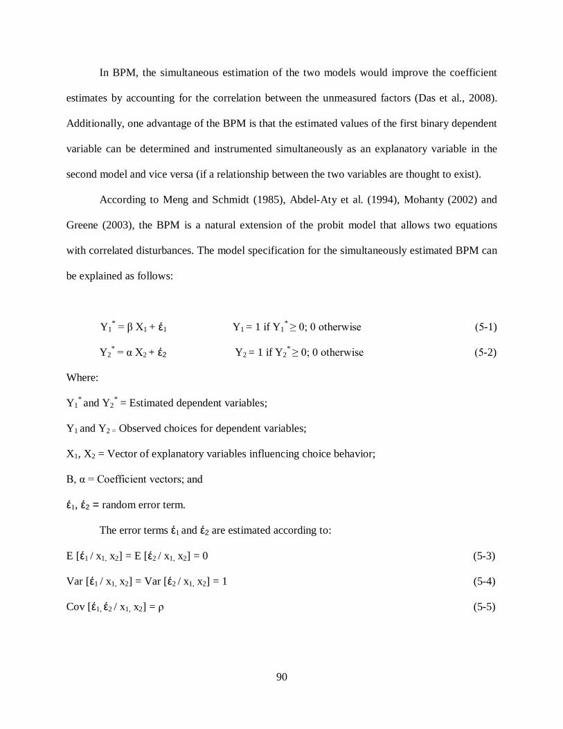
90

In BPM, the simultaneous estimation of the two models would improve the coefficient

estimates by accounting for the correlation between the unmeasured factors (Das et al., 2008).

Additionally, one advantage of the BPM is that the estimated values of the first binary dependent

variable can be determined and instrumented simultaneously as an explanatory variable in the

second model and vice versa (if a relationship between the two variables are thought to exist).

According to Meng and Schmidt (1985), Abdel-Aty et al. (1994), Mohanty (2002) and

Greene (2003), the BPM is a natural extension of the probit model that allows two equations

with correlated disturbances. The model specification for the simultaneously estimated BPM can

be explained as follows:

Y1* = β X1

+ έ1 Y1 = 1 if Y1* ≥ 0; 0 otherwise (5-1)

Y2* = α X2 + έ2 Y2 = 1 if Y2

* ≥ 0; 0 otherwise (5-2)

Where:

Y1* and Y2

* = Estimated dependent variables;

Y1 and Y2 = Observed choices for dependent variables;

X1, X2 = Vector of explanatory variables influencing choice behavior;

Β, α = Coefficient vectors; and

έ1, έ2 = random error term.

The error terms έ1 and έ2 are estimated according to:

E [έ1 / x1, x2] = E [έ2 / x1, x2] = 0 (5-3)

Var [έ1 / x1, x2] = Var [έ2 / x1, x2] = 1 (5-4)

Cov [έ1, έ2 / x1, x2] = ρ (5-5)

91

Where: ρ is the correlation coefficient between the two error terms. If ρ equals zero, the bivariate

probit model converges to two separate binomial probit models. In addition, the model

parameters of the two probit equations are estimated simultaneously using full information

maximum likelihood estimation. Parameters vectors Β, α, and ρ are estimated to maximize the

likelihood function. Also, significant ρ will imply the presence of unobserved individual factors

(heterogeneity) that affect both dependent variables used in the BPM.

Three bivariate probit models were developed after investigating several alternative

model formations and dependent variables (as shown in Table 5-7). Drivers’ response to VSL

signs at heavy fog and medium-high traffic volume (0 if do nothing or follow other vehicles’

speed, 1 if reduce speed or reduce speed and put blinkers on) was the first dependent variable in

the three models. The second dependent variables in the three fitted BPM were drivers’ response

to VSL signs at very light fog and low traffic volume (0 if do nothing, 1 if reduce speed or

reduce speed and put blinkers on), drivers’ response to CMS at low traffic volume (0 if do

nothing or reduce speed after some time, 1 if reduce speed immediately or reduce speed and put

blinkers on), and drivers’ response to CMS at medium-high traffic volume (0 if do nothing or

reduce speed after some time or follow other vehicles’ speed, 1 if reduce speed immediately or

reduce speed and put blinkers on), respectively. Level 0 was considered the base case for each

dependent variable (Table 5-7).

The results of the three BPM revealed that gender, age, drivers’ familiarity with VSL

signs, and road type were the most significant factors affecting the likelihood of reducing speed

following the instructions of VSL or CMS in response to adverse visibility conditions.

Table 5-7: Summary of Bivariate probit models (a Base case b Akaike Information Criterion)

First BPM Model Second BPM Model Third BPM Model

Variable Description Estimate Standard Error P-value Estimate Standard

Error P-value Estimate Standard Error P-value

First equation drivers’ responses to VSL signs at heavy fog and medium-high traffic condition (Baseline: do nothing or follow other vehicles’ speed)

Intercept 0.6629 0.1290 0.0000 0.6896 0.1325 0.0000 0.6826 0.1299 0.0000 Gender - male ----- a ----- a ----- a

Gender - female 0.5889 0.1702 0.0005 0.5569 0.1748 0.0014 0.5747 0.1711 0.0008 Age (18-25) ----- a ----- a ----- a Age (36-50) 0.6515 0.2311 0.0048 0.6219 0.2289 0.0066 0.6283 0.2232 0.0049 Age (+51) 0.6556 0.2280 0.0040 0.6036 0.2180 0.0056 0.6239 0.2186 0.0043

Drivers’ familiarity with VSL SIGNS (no) ----- a ----- a ----- a Drivers’ familiarity with VSL SIGNS (yes) 0.5233 0.2045 0.0105 0.4807 0.2168 0.0266 0.5193 0.2075 0.0123

Road type (2-lane road) ----- a ----- a ----- a Road type (freeway) -0.3805 0.2077 0.0670 -0.3319 0.2141 0.1212 -0.3923 0.2175 0.0713

Second equation

Drivers’ responses to VSL signs at very light fog and low

traffic volumes (Baseline: do nothing)

Drivers’ responses to CMS at low traffic volume

(Baseline: do nothing or reduce speed after some time)

Drivers’ responses to CMS at medium-high traffic volume

(Baseline: do nothing or reduce speed after some time or follow

other vehicles’ speed) Intercept -0.2175 0.1032 0.0350 -1.0576 0.1241 0.0000 -0.4799 0.1149 0.0000

Gender-male ----- a ----- a ----- a Gender-female 0.2265 0.1166 0.0520 0.2758 0.1128 0.0145 0.3346 0.1141 0.0034

Age (18-25) ----- a ----- a ----- a Age (26-35) 0.4105 0.1468 0.0052 0.6540 0.1630 0.0001 0.6486 0.1534 0.0000 Age (36-50) 0.5372 0.1483 0.0003 0.6067 0.1588 0.0001 0.6419 0.1506 0.0000 Age (+51) 1.2097 0.1673 0.0000 1.2299 0.1589 0.0000 1.2226 0.1567 0.0000

Road type (2-lane road) ----- a Road type (freeway) -0.2973 0.1139 0.0091

Error terms correlation coefficient (ρ) 0.3534 0.0899 0.0001 0.3819 0.1149 0.0009 0.3785 0.0969 0.0001

Number of observations 566 566 566

Log-likelihood at convergence -499.475 -500.666 -510.442

AIC b 1020.95 1023.332 1044.884

93

In addition, to improve our understanding of the factors affecting drivers’ behavior at

different visibility and traffic conditions, an MPM was developed. Based on the three BPM

mentioned above, it was found that the dependent variables that better explain drivers’ response

to adverse visibility conditions were; drivers’ response to VSL at heavy fog and medium-high

traffic volume, drivers’ response to VSL at very light fog and low traffic volume, and drivers’

response to CMS at medium-high traffic volume. Therefore, these three dependent variables

were used in MPM.

The MPM estimates, goodness-of-fit statistics, and the correlation coefficient “ρ”

between every two error terms in the three equations are presented in Table 5-8. As shown in

Table 5-8, the coefficients of correlation “ρ” is statistically different from zero, hence illustrating

the validity of using the Multivariate probit framework.

According to the first model, while encountering a heavy fog condition and some

vehicles are ahead (medium-high traffic volume), the likelihood of female drivers who are

reducing their speed or reducing their speed and putting the blinkers on are more than the

corresponding male drivers. This implies that female drivers are more cautious than male drivers.

Concerning age, as age increases, the likelihood of following VSL instruction at heavy

fog and medium-high traffic volume increases. The results suggest that compared to young

respondents (18-25 years old), old respondents (51 years old or more) are more likely to reduce

their speed following VSL instruction. This indicates that maturity and experience are essential

factors that affect the driver’s response to VSL instructions.

An expected finding is that drivers, who are familiar with VSL signs, are more likely to

reduce their speed at heavy fog conditions. This could be attributed to the fact that drivers, who

94

are familiar with VSL signs and aware of its importance in avoiding a potential accident in case

of reduced visibility due to FS, are less likely to ignore its instructions.

Regarding the type of road, at 90% confidence, the probability of reducing speed,

following VSL at heavy fog and medium-high traffic volume while driving on a freeway, is less

than the corresponding probability while driving on a two-lane road. Thus drivers could be more

cautious on two-lane roads.

Similar findings were obtained from the second and third equations. The second model

suggests that both females and old drivers (51 years old or more) are more likely to reduce their

speed following VSL instructions at very light fog and low traffic volume compared to males

and young drivers (18-25 years old), respectively.

According to the third probit model, while encountering CMS at medium-high traffic

volume which advise drivers to reduce their speed due to reduction of visibility, the likelihood of

females and old drivers who are reducing their speed or reducing their speed and putting blinkers

on are more than the corresponding males and young drivers. Again, this implies that females

and old drivers are more cautious than male and young drivers.

Finally, drivers who drive on a freeway at poor visibility conditions are less likely to

respond to CMS instructions compared to those who drive on a two-lane road possibly due to

more cautious driving on two-lane roads. It is possible that the presence of medians on freeways

could give drivers a better sense of protection from the opposing traffic.

95

Table 5-8: Multivariate Probit model estimates (a Base case b Akaike Information Criterion)

Variable Description Estimate Standard Error P-value

First equation : drivers’ responses to VSL signs at heavy fog and medium-high traffic volume (Baseline: do nothing or follow other vehicles’ speed) Intercept 0.5690 0.1463 0.0001

Gender-male ----- a Gender-female 0.5553 0.1714 0.0012

Age (18-25) ----- a Age (26-35) 0.2778 0.1712 0.1041 Age (36-50) 0.7678 0.2408 0.0014 Age (+51) 0.7637 0.2356 0.0012

Drivers’ familiarity with VSL SIGNS (no) ----- a Drivers’ familiarity with VSL SIGNS (yes) 0.5001 0.2106 0.0176

Road type (2-lane road) ----- a Road type (freeway) -0.3508 0.2193 0.1097

Second equation : drivers’ responses to VSL signs at very light fog and low traffic volume (Baseline: do nothing)

Intercept -0.2299 0.1038 0.0267 Gender-male ----- a

Gender-female 0.2242 0.1174 0.0562 Age (18-25) ----- a Age (26-35) 0.4501 0.1527 0.0032 Age (36-50) 0.5589 0.1496 0.0002 Age (+51) 1.2241 0.1679 0.0000

Third equation : drivers’ responses to CMS at medium-high traffic volume (Baseline: do nothing or reduce speed after some time or follow other vehicles’ speed)

Intercept -0.5007 0.1155 0.0000 Gender-male ----- a

Gender-female 0.3321 0.1146 0.0038 Age (18-25) ----- a Age (26-35) 0.6880 0.1569 0.0000 Age (36-50) 0.6574 0.1510 0.0000 Age (+51) 1.2322 0.1571 0.0000

Road type (2-lane road) ----- a Road type (freeway) -0.2694 0.1138 0.0179

Error terms correlation coefficient between equations 1 & 2 (ρ12) 0.3525 0.0901 0.0001

Error terms correlation coefficient between equations 1 & 3 (ρ13) 0.3716 0.0976 0.0001

Error terms correlation coefficient between equations 2 & 3 (ρ23) 0.2524 0.0698 0.0003

Number of observations 566

Log-likelihood at convergence -835.7581

AIC b 1707.5162

96

5.5 Structural Equation Modeling (SEM) Approach

This section examine drivers’ responses under low visibility conditions and quantify the

impacts and values of various factors found to be related to drivers’ compliance and drivers’

satisfaction with VSL and CMS instructions in different visibility, traffic conditions, and at two

types of roadways; freeways and two-lane roads. To achieve these goals, Explanatory Factor

Analysis (EFA) and Structural Equation Modeling (SEM) approaches were adopted.

5.5.1 Explanatory Factor Analysis

Explanatory Factor Analysis (EFA) is a statistical method used to identify the number

and nature of the underlying factors (latent variables) that are responsible for the variability in

the data. Table 5-9 shows description and input codes of the observed variables used in the

present study.

These variables include (1) demographic variables (i.e., gender, age, number of years the

driver had a valid driver’s license, number of traffic citations in the previous 3 years,

involvement in fog/smoke or heavy rain related crashes, and frequency usage of freeways/ two-

lane roads), (2) roadway type (the type of survey that each participate responded to: freeways or

2 lane roads), (3) familiarity with CMS and VSL signs, (4) drivers’ satisfaction with the

importance of using CMS and VSL signs in reduced visibility conditions, (5) drivers’ responses

to CMS instructions under two traffic conditions (no car leading ahead and some vehicles are

ahead), (6) drivers’ responses to VSL instructions under four levels of fog (very light, light,

medium and heavy) and the same two traffic conditions mentioned above.

97

It is worth mentioning that nominal variables (such as CMS_follow 1 and CMS_follow

2) were transferred to binary variables. In SEM, this way is preferable as it allow us to indentify

the nonlinear influence of nominal variables on endogenous variables (Lee et. al, 2008). Using

SAS procedure FACTOR, EFA was performed on the observed variables shown in Table 5-9.

The Scree test, a plot of the eigenvalues associated with factor analysis, suggests that the number

of meaningful factors to retain is four.

In addition, Table 5-10 shows the Varimax (orthogonal) rotated factor loadings which are

the correlations between each observed variable (rows) and each factor (columns). In interpreting

the rotated factor pattern, usually a variable is said to load on a given factor if the factor loading

is 0.4 or greater for that factor (Hatcher 1994 and Lee et. al, 2008). Using these criteria, four

factors were identified. Three observed variables (VSL_follow 1, VSL_follow 5 and

VSL_follow 6) were found to load on the first factor, which was subsequently labeled “drivers’

compliance with VSL signs under very light/light fog”. Also, three variables (VSL_follow 3,

VSL_follow 4, and VSL_follow 8) loaded on the second factor, which was called “drivers’

compliance with VSL signs under medium/heavy fog”. In addition, four variables (Intention,

CMS_satisfaction, VSL_satisfaction, and CMS_satisfaction2) loaded on the third factor which

was labeled “satisfaction with VSL and CMS signs”. Finally, two variables (age and

driving_exp) loaded on the fourth factor which was called “driver factors”. These four factors

account for about 97% of the variance in the data. It is worth noting that two variables

(VSL_follow 2 and VSL_follow 7) load on both factors 1 and 2 and hence, they were not used in

interpreting the factors.

98

Table 5-9: Definitions of variable, their codes and statistics

Observed variables Description and coding of input value

Simple Statistics

Name Description Mean S.D

Gender Gender 1 male 0 female 0.55 0.50

Age Age Continuous variable 37.03 15.31

Driving_exp Driving experience (number of years the driver had a valid driver’s license) Continuous variable 19.30 14.58

Citation_no Number of traffic citations in the previous 3 years Continuous variable 0.66 1.28

FS_crashes Involvement in fog/smoke related crashes 1 Yes 0 No 0.04 0.19

HV_crashes Involvement in heavy rain related crashes 1 Yes 0 No 0.11 0.31

Exposure Frequency usage of freeways/ two-lane roads

1 rarely or never 2 once a month 3 once in two weeks 4 once a week 5 2-4 times a week 6 > 4 times a week

4.93 1.44

Road_type The type of survey that a participant responded to 1 two-way lane roads 0 freeways 0.54 0.50

CMS_ familiarity Drivers’ familiarity with changeable message signs 1 Yes

0 No 0.84 0.37

VSL_ familiarity Drivers’ familiarity with variable speed limit signs 1 Yes

0 No 0.68 0.47

Intention Willingness to follow VSL and CMS instructions 1 Strongly disagree 2 disagree 3 neither agree nor

disagree 4 agree 5 strongly agree

4.42 0.683 CMS_

satisfaction Drivers’ satisfaction with the usefulness of CMS in warning them about reduced visibility conditions 4.39 0.68

VSL_ satisfaction

Drivers’ satisfaction with the usefulness of VSL in informing them about safe speed limit under reduced visibility conditions

3.97 0.99

CMS_ Satisfaction 2

Drivers’ satisfaction with the usefulness of using two successive CMS prior to fog/smoke zones 4.14 0.88

CMS_follow 1 Drivers’ responses to CMS at light fog condition and no car leading ahead

1 reduce speed immediately or reduce speed and put blinkers on

0 other

0.38 0.49

CMS_follow 2 Drivers’ responses to CMS at light fog condition and some vehicles are ahead

0.54 0.50

VSL_follow 1 Drivers’ responses to VSL at very light fog and no car leading ahead

Continuous variables (% of reduction of speed

following VSL instructions)

19.97 18.10

VSL_follow 2 Drivers’ responses to VSL at light fog and no car leading ahead 24.60 17.24

VSL_follow 3 Drivers’ responses to VSL at medium fog and no car leading ahead 35.29 12.83

VSL_follow 4 Drivers’ responses to VSL at heavy fog and no car leading ahead 42.14 10.58

VSL_follow 5 Drivers’ responses to VSL at very light fog and some vehicles are ahead 16.16 19.82

VSL_follow 6 Drivers’ responses to VSL at light fog and some vehicles are ahead 18.58 20.25

VSL_follow 7 Drivers’ responses to VSL at medium fog and some vehicles are ahead 31.41 19.04

VSL_follow 8 Drivers’ responses to VSL at heavy fog and some vehicles are ahead 40.76 16.85

99

Table 5-10: Varimax rotated factor analysis results

Factor 1 Factor 2 Factor 3 Factor 4 Age 31 10 15 93 * Driving_exp 28 5 12 90 * Citation_no -10 -8 -3 -24 Gender -10 -6 -18 -7 FS_crashes 0 -1 1 9 HV_crashes -1 -9 -3 7 Exposure -2 1 -2 15 Road type 1 30 -7 -11 CMS_familiarity 0 -11 2 8 VSL_familiarity 7 -7 16 16 Intention 15 12 58 * 3 CMS_satisfaction 9 10 76 * 3 VSL_satisfaction 15 8 62 * -2 CMS_Satisfaction 2 7 9 57 * 0 CMS_Follow1 33 32 37 15 CMS_Follow2 34 27 39 18 VSL_Follow1 67 * 35 26 13 VSL_Follow2 59 * 49 * 25 17 VSL_Follow3 39 79 * 19 16 VSL_Follow4 25 82 * 13 15 VSL_Follow5 92 * 14 23 8 VSL_Follow6 91 * 19 21 12 VSL_Follow7 52 * 51 * 24 11 VSL_Follow8 30 58 * 23 18 Printed values are multiplied by 100 and rounded to the nearest integer. Values greater than 0.4 are flagged by an '*'.

5.5.2 Reliability Analysis

Cronbach’s α (alpha) is a coefficient of consistency that measures how well a set of

variables or items measures a single, unidirectional latent construct (Ma et al. 2010). Cronbach’s

alpha generally increases when the correlations between the items increase. For this reason, it is

called the internal consistency or the internal consistency reliability of the test. Moreover,

composite reliability is analogous to the coefficient alpha, and reflects the internal consistency of

the indicators measuring a given factor (Hatcher 1994).

100

In this survey study, Cronbach’s alpha was applied to evaluate the internal consistency of

the four latent factors obtained by EFA. The values of Cronbach’s alpha of the observed

variables as well as composite reliability of the latent variables are given in Table 5-11. A

Cronbach’s alpha of 0.7 or more indicates acceptable reliability (Nunnally 1978, Hatcher 1994

and Ma et al. 2010). As shown in Table 5-11, the reliability of the scales is generally acceptable.

This implies that the used scales (latent variables) are valid.

Table 5-11: Cronbach’s α-value of latent and observed variables

Latent variable Observed variable Reliability

Cronbach’s α Composite reliability

Drivers’ compliance with VSL at very light

/ light fog (F1)

VSL_follow 1 0.957 0.919 VSL_follow 5 0.838

VSL_follow 6 0.841 Drivers’ compliance

with VSL at medium / heavy fog (F2)

VSL_follow 3 0.750 0.839 VSL_follow 4 0.726

VSL_follow 8 0.881

Satisfaction with VSL/CMS (F3)

Intention 0.708

0.720 CMS_Satisfaction 0.716 VSL_Satisfaction 0.773 CMS_Satisfaction 2 0.704

Driver factors (F4)

Age 0.842

0.740 Driving exp. 0.814 Citation_no. 0.747 Exposure 0.723

101

5.5.3 Structural Equation Modeling

Structural Equation Modeling (SEM) represents a combination of two types of statistical

techniques: factor analysis and simultaneous equation models. In SEM, variables can be either

exogenous or endogenous which allow SEM to handle indirect, multiple, and reverse

relationships (Martinez et. al 2010).

SEM is a technique that consists of a set of equations that are specified by direct links

between variables and hence it can be called “the simultaneous equations”. However, in SEM,

latent variables (unobserved or unmeasured variables) can be introduced (Lee et al. 2008).

The advantages of using SEM include: (1) it can handle complex relationships among

variables, where some variables can be hypothetical or unobserved (latent variables); (2) It

estimates all coefficients in the model simultaneously and thus, one is able to assess the

significance and strength of a particular relationship in the context of the complete model, (3)

multi-colinearity can be accounted for, (4) when using latent variables in SEM, measurement

error is eliminated and thus more valid coefficients are obtained (Dion, 2008 and Martinez et. al,

2010). Therefore, SEM is an adequate tool to model the complex relationships such as those that

are being modeled in this survey study. SEM is applied in this research using SAS software

(version 9.2) procedure CALIS.

To develop SEM, the present analysis followed a two-step approach recommended by

Anderson and Gerbing (1988). With this approach, the first step involves using confirmatory

factor analysis (CFA) to develop an acceptable measurement model. This measurement model

describes the nature of the relationship between a number of latent variables and the observed

variables that measure those latent variables. However, this measurement model does not specify

any causal relationships between the latent variables of interest.

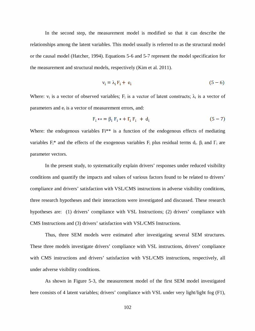
102

In the second step, the measurement model is modified so that it can describe the

relationships among the latent variables. This model usually is referred to as the structural model

or the causal model (Hatcher, 1994). Equations 5-6 and 5-7 represent the model specification for

the measurement and structural models, respectively (Kim et al. 2011).

Where: vi is a vector of observed variables; Fi is a vector of latent constructs; λi is a vector of

parameters and ei is a vector of measurement errors, and:

Where: the endogenous variables Fi** is a function of the endogenous effects of mediating

variables Fi* and the effects of the exogenous variables Fi plus residual terms di. βi and Γi are

parameter vectors.

In the present study, to systematically explain drivers’ responses under reduced visibility

conditions and quantify the impacts and values of various factors found to be related to drivers’

compliance and drivers’ satisfaction with VSL/CMS instructions in adverse visibility conditions,

three research hypotheses and their interactions were investigated and discussed. These research

hypotheses are: (1) drivers’ compliance with VSL Instructions; (2) drivers’ compliance with

CMS Instructions and (3) drivers’ satisfaction with VSL/CMS Instructions.

Thus, three SEM models were estimated after investigating several SEM structures.

These three models investigate drivers’ compliance with VSL instructions, drivers’ compliance

with CMS instructions and drivers’ satisfaction with VSL/CMS instructions, respectively, all

under adverse visibility conditions.

As shown in Figure 5-3, the measurement model of the first SEM model investigated

here consists of 4 latent variables; drivers’ compliance with VSL under very light/light fog (F1),

103

drivers’ compliance with VSL under medium/heavy fog (F2), satisfaction with VSL/CMS (F3)

and driver factors (F4). These four latent variables (represented by Fi in Equation 5-6) are

measure by 14 observed variables (represented by vi in Equation 5-6).

Although the results of EFA showed that only two variables (age and driving experience)

are loaded on the fourth latent variable (F4), several demographic observed variables were

investigated in the measurement model because prior studies indicated that it is highly desirable

to have at least three variables loading on each latent variable (Spector 1992 and Hatcher 1994).

As shown in Figure 5-3, the results revealed that each of F1 and F2 is measured by three

observed variables. However, each of F3 and F4 is measured by four observed variables. As

indicated earlier, the descriptions of these variables are provided in Table 5-9. As shown in

Figure 5-3, rectangles represent observed variables; ellipses represent unobserved latent

variables and arrows pointing from the observed variables to latent factors representing

regression paths. Additionally, circles with an arrow pointing toward each observed variable

represents the measurement error terms (represented by ei in Equation 5-6). Moreover, each

latent factor is connected to every other factor by a curved two-headed arrow meaning that every

factor is allowed to covary with every other factor.

Standardized loading factors along with its standard error and t-value are shown in Figure

5-3. In the Figure, the numbers on the arrows are parameter estimates and numbers in

parentheses indicate standard errors and t-values. The t values presented in Figure 5-3 represent

large-sample t tests of the null hypothesis that the factor loading is equal to zero in the

population. The obtained t values showed that all factor loadings were significant at 95%

confidence (t-values are greater than 1.96).

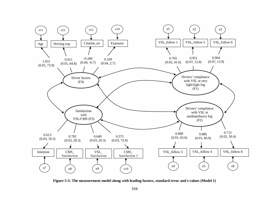
104

Figure 5-3: The measurement model along with loading factors, standard error and t-values (Model 1)

Age Driving exp. Citation_no

Intention CMS_ Satisfaction

VSL_ Satisfaction

CMS_ Satisfaction 2

VSL_follow 1 VSL_follow 5 VSL_follow 6

VSL_follow 3 VSL_follow 4 VSL_follow 8

Exposure

0.765 (0.02, 41.6)

0.951 (0.07, 12.8)

0.964 (0.07, 13.9)

0.898 (0.01, 63.6)

0.886 (0.01, 60.9)

0.712 (0.02, 30.4) 0.613

(0.03, 18.3) 0.785

(0.03, 28.3) 0.649

(0.03, 20.3) 0.575

(0.03, 73.9)

1.031 (0.01, 73.9)

0.911 (0.01, 64.8)

-0.260 (0.04, -6.7)

0.109 (0.04, 2.7)

e1

Drivers’ compliance with VSL at very

light/light fog (F1)

Drivers’ compliance with VSL at

medium/heavy fog (F2)

e4 e7

e13 e14 e12 e11

Driver factors (F4)

Satisfaction with

VSL/CMS (F3)

e2 e3

e6 e5 e8 e9 e10

105

Regarding the structural model, Figure 5-4 presents the first SEM model that examines

drivers’ compliance with VSL instructions under different fog conditions. This model was first

conceptualized so that it could be refined through SEM. This model was composed based on the

relation on the correlations between observed variables and latent variables, as well as

correlations among latent variables. As shown in Figure 5-4, the first SEM model consists of the

same four latent variables in addition to one observed variable; roadway type (2-lane roads vs.

freeway). It was decided to examine the effect of roadway type on drivers’ behaviors because our

preliminary analysis indicated that there is a significant correlation between the type of road and

drivers’ behavior under reduced visibility conditions (Hassan et al. 2011).

It is worth mentioning that each latent variable is an unobserved variable that has no

established unit of measurement. Therefore, to define the unit of measurement of each latent

variable, a non-zero coefficient (usually one) is given to one of its observed variables as an

indicator (i.e., reference variable). For that reason, the factor loading of the indicator variable

that best represent the corresponding latent variable was fixed at 1 (Hatcher, 1994 and Lee et al.

2008). The final structure of the first SEM model as well as standardized loading factors,

standard errors and t-values are given in Figure 5-4. According to the results of first SEM model

shown in Figure 5-4, it was found that drivers’ satisfaction with VSL/CMS was the most

significant factor that positively affected drivers’ compliance with VSL under very light or light

fog (factor loading=0.372, t-value=9.182). In addition, driver factors (i.e., higher age, longer

driving experience, less number of traffic citations and higher usage of freeways/2-lane roads)

was found out to positively affect drivers’ responses to VSL instructions under very light or light

fog (factor loading = 0.351, t-value = 9.637).

106

Figure 5-4: Structural equation model of drivers’ compliance with VSL instructions (Model 1) a: (Estimates for variance of exogenous variables (i.e., latent, observed, error or disturbance)

0.69a

Age Driving exp Citation_no

Driver factors (F4)

Intention CMS_

Satisfaction

Satisfaction with VSL/CMS (F3)

VSL_ Satisfaction

CMS_ Satisfaction 2

Road type

VSL_follow 1

Drivers’ compliance with VSL at very light

/ light fog (F1)

Drivers’ compliance with VSL at medium /

heavy fog (F2)

VSL_follow 5 VSL_follow 6

VSL_follow 3 VSL_follow 4 VSL_follow 8

0.351 (0.04, 9.64)

.956 1

1 .922 .715

1 .919 -0.26

1 .617 .573

0.253 (0.04, 6.74)

0.341 (0.04, 8.06)

0.231 (0.05, 5.10)

Exposure

.763 .118

0.051 (0.04, 1.39)

R2=0.32

R2=0.31

0.95a

1.00a

1.00a

Standardized path coefficient (S.E, t-value)

0.68a

0.372 (0.04, 9.18)

.649

0.335 (0.04, 8.88)

107

However, roadway type (i.e., driving on 2-lane roads vs. freeways) had no direct effect

(the hypothesis was rejected as shown in Table 5-12) on drivers’ compliance with VSL

instructions under very light or light fog (factor loading = 0.051, t-value = 1.389).

Similarly, the results indicated that drivers’ satisfaction with VSL/CMS positively

affected drivers’ behavior (following VSL instructions) under medium or heavy fog (factor

loading=0.341, t-value=8.056). Also, driver factors was found out to positively affect drivers’

responses to VSL instructions under medium or heavy fog (factor loading = 0.335, t-value =

8.875). Moreover, it was found that roadway type positively affected drivers’ compliance with

VSL instructions under medium or heavy fog (factor loading = 0.253, t-value = 6.737). This

imply that drivers tend to follow VSL instructions under medium or heavy fog while driving on

2-lane roads compared to driving on freeways possibly due to the absence of medians.

In addition, the results revealed that driver factors has indirect effect on drivers’

responses to VSL instructions under reduced visibility conditions as it positively affected

drivers’ satisfaction with VSL/CMS which subsequently positively affected drivers’ compliance

with VSL instructions under adverse visibility conditions (factor loading = 0.231, t-value =

5.102).

Finally, the first SEM model explained 31% and 32% of total variance in drivers’

compliance with VSL under very light/light fog conditions and drivers’ compliance with VSL

under medium/heavy fog conditions, respectively.

108

As mentioned earlier, the second SEM model (shown in Figure 5-5) was adopted to

examine causal relationships between drives’ compliance with warning messages displayed on

CMS under reduced visibility conditions and its associated factors. The standardized path

coefficients, standard errors and its t-values are presented in Figure 5-5. The results of the second

SEM model suggest that drivers’ satisfaction with VSL/CMS was the most significant variable

that positively affected drivers’ compliance with CMS instructions under reduced visibility in

both traffic conditions; (1) no car leading ahead and (2) some vehicles are ahead. In addition, it

was found that driver factors positively affected drivers’ compliance with CMS instructions in

both traffic conditions. This result implies that drivers with higher driving experience, less

number of traffic citations and higher usage of freeways/2-lane roads are more likely to obey

warning messages displayed on CMS under reduced visibility conditions.

Additionally, driver factors positively affected drivers’ satisfaction with VSL/CMS.

Moreover, the findings revealed that roadway type was found out to positively affect drivers’

compliance with CMS only when some vehicles are ahead. This result indicates that when

driving on 2-lane roads and some vehicles are ahead, drivers tend to follow CMS instructions

compared to driving on freeways. However, when no leading vehicles are ahead, roadway type

has insignificant effect on drivers’ compliance with CMS instructions.

The second SEM model explained 29% and 28% of the total variance in drivers’

compliance with CMS instructions when no car is leading ahead and drivers’ compliance with

CMS instruction when some vehicles are ahead, respectively.

It is worth mentioning that it was decided to study drivers’ responses to CMS under two

traffic conditions and under only one reduced visibility condition (light fog) to reduce the

number of survey questions.

109

One interesting research hypothesis was to examine whether drivers’ behavior in

response to VSL/CMS instructions was affected by the survey method. The hypothesis that the

survey method significantly affected drivers’ response to VSL/CMS instructions was rejected at

the 5% level of significance.

110

Figure 5-5: Structural equation model of drivers’ compliance with CMS instructions (Model 2) a: (Estimates for variance of exogenous variables (i.e., latent, observed, error or disturbance)

Age Driving exp Citation_no

Intention CMS_ Satisfaction

Satisfaction with VSL/CMS (F1)

VSL_ Satisfaction

CMS_ Satisfaction 2

(CMS_Follow 1) Drivers’ compliance with

CMS when no leading vehicles are ahead

0.244 (0.04, 6.54)

1 .918 -0.261

1 .624 .562 .650

0.421 (0.04, 10.56)

0.425 (0.04, 10.71)

0.232 (0.04, 5.15)

Exposure

.116

(CMS_Follow 2) Drivers’ compliance with CMS when some vehicles

are ahead

Standardized path coefficient (S.E, t-value)

0.71a

R2=0.28

R2=0.29

0.72a 0.95a

1.0a

1.0a

Road type

Driver factors (F2)

0.092 (0.04, 2.49)

0.237 (0.04, 6.37)

0.053 (0.04, 1.45)

111

The third SEM model developed in this research aimed to examine factors associated

with drivers’ satisfaction with VSL/CMS instructions. The results (shown in Figure 5-6)

indicated that driver factors positively affected drivers’ satisfaction with VSL/CMS (factor

loading=0.201, t-value=4.4). These results imply that older motorists (experienced drivers) are

more satisfied with the usefulness of warning messages/advice displayed on VSL/CMS signs

compared to young drivers. In addition, drivers who got traffic citation within the last three years

are less satisfied with VSL/CMS. As expected, the results showed that drivers with higher usage

of freeways/2 lane roads are more satisfied with VSL/CMS possibly due to the fact that those

drivers encounter these signs on daily bases and thus, they are more familiar and satisfied with

the role of VSL/CMS in improving safety.

The results also revealed that familiarity with VSL signs positively affected drivers’

satisfaction with VSL/CMS (factor loading=0.115, t-value=2.46). However, familiarity with

CMS was found to have insignificant effect on drivers’ satisfaction with VSL/CMS. One

possible explanation is that drivers in Central Florida are more familiar with CMS compared to

VSL and hence, drivers, who are familiar with VSL signs, usually are aware of its importance for

safety. Again, the results indicated that driver factors has a significant positive effect on

familiarity with VSL signs (factor loading=0.186, t-value=4.64). This is logical as older drivers

(or experienced drivers) are more familiar with VSL signs compared to young (novel) drivers.

Finally, the third SEM model explained 36% of total variance in drivers’ satisfaction with

VSL/CMS. Table 5-12 summarizes the verification of the research hypotheses of the three SEM

models investigated in the present study. The verification of these hypotheses was developed

based on the t-values that were estimated for each of the paths between the observed and latent

variables.

112

Figure 5-6: Structural equation model of drivers’ satisfaction with VSL/CMS instructions (Model 3) a: (Estimates for variance of exogenous variables (i.e., latent, observed, error or disturbance)

Age Driving exp. Citation_no.

Driver factors (F2)

Familiarity with VSL

CMS_ Satisfaction

0.96

0.64a

0.064

0.186 (0.04, 4.64)

Intention

VSL_ Satisfaction

CMS_ Satisfaction 2

Familiarity with CMS

0.115 (0.04, 2.46)

Standardized path coefficient (S.E, t-value)

-0.053 .598 1 .636 .579

-0.262 .920 1

R2 =0.36

Exposure

1.0a

.114

Satisfaction with VSL/CMS

(F1) 0.201

(0.04, 4.4)

113

Table 5-12: Verification of the three SEM models hypotheses

Hypothesis

Est

imat

e

Stan

dar

d er

ror

t-va

lue

a

rem

arks

Mod

el 1

H1 Driver factors will have a positive effect on drivers’ compliance with VSL instructions under very light or light fog 0.351 0.036 9.637 Accept

H2 Drivers’ satisfaction with VSL/CMS will have a positive effect on drivers’ compliance with VSL instructions under very light or light fog

0.372 0.041 9.182 Accept

H3 Roadway type will have a positive effect on drivers’ compliance with VSL instructions under very light or light fog 0.051 0.037 1.389 Reject

H4 Driver factors will have a positive effect on drivers’ compliance with VSL instructions under medium or heavy fog 0.335 0.038 8.875 Accept

H5 Drivers’ satisfaction with VSL/CMS will have a positive effect on drivers’ compliance with VSL instructions under medium or heavy fog

0.341 0.042 8.056 Accept

H6 Roadway type will have a positive effect on drivers’ compliance with VSL instructions under medium or heavy fog 0.253 0.038 6.737 Accept

H7 Driver factors will have a positive effect on drivers’ satisfaction with VSL/CMS 0.231 0.045 5.102 Accept

Mod

el 2

H8 Driver factors will have a positive effect on drivers’ compliance with CMS instructions when no leading vehicles are ahead 0.244 0.037 6.544 Accept

H9 Drivers’ satisfaction with VSL/CMS will have a positive effect on drivers’ compliance with CMS instructions when no leading vehicles are ahead

0.421 0.039 10.564 Accept

H10 Roadway type will have a positive effect on drivers’ compliance with CMS instructions when no leading vehicles are ahead 0.053 0.037 1.450 Reject

H11 Driver factors will have a positive effect on drivers’ compliance with CMS instructions when some vehicles are ahead 0.237 0.037 6.369 Accept

H12 Drivers’ satisfaction with VSL/CMS will have a positive effect on drivers’ compliance with CMS instructions when some vehicles are ahead

0.425 0.040 10.711 Accept

H13 Roadway type will have a positive effect on drivers’ compliance with CMS instructions when some vehicles are ahead 0.092 0.036 2.491 Accept

H14 Driver factors will have a positive effect on drivers’ satisfaction with VSL/CMS 0.232 0.045 5.151 Accept

Mod

el 3

H8 Driver factors will have a positive effect on drivers’ satisfaction with VSL/CMS instructions 0.201 0.046 4.404 Accept

H16 Drivers’ familiarity with CMS has a positive effect on drivers’ satisfaction with VSL/CMS instructions -0.05 0.046 -1.146 Reject

H17 Drivers’ familiarity with VSL has a positive effect on drivers’ satisfaction with VSL/CMS instructions 0.115 0.047 2.456 Accept

H18 Driver factors will have a positive effect on drivers’ familiarity with CMS 0.064 0.042 1.516 Reject

H19 Driver factors will have a positive effect on drivers’ familiarity with VSL 0.186 0.040 4.643 Accept

114

5.5.4 SEM Models Fit Indices

A widely reported goodness of fit index used in SEM analysis is the Chi-square test

which provides a test of the null hypothesis that the theoretical model fit the data. If the model

fits the data well, Chi-square value should be small and p-value associated with the Chi-square

should be relatively large. However, with large samples, the Chi-square statistic will very

frequently be increased even if the SEM model provides a good fit (James et al. 1982, Hatcher

1994, Acker and Witlox 2010).

For this reason, prior studies recommended to supplement the Chi-square with some

alternative model fit indices. Some commonly fit indices are; Goodness of Fit Index (GFI),

Adjusted Goodness of Fit Index (AGFI), Comparative Fit Index (CFI), Normed Fit Index (NFI),

Non-Normed Fit Index (NNFI), Root Mean Square Error of Approximation (RMSEA).

Table 5-13 shows the goodness of fit statistics of the three SEM models that are

presented in this section. As shown in Table 5-13, the models displayed values greater than 0.9

on GFI, AGFI, CFI, NFI, NNFI and a value smaller than 0.05 on RMSEA, indicative of a good

fit (Bentler & Bonett 1980, Hatcher 1994, Lee et al. 2008, 2009 and Ma et al. 2010).

Table 5-13: Fit statistics for structural equation models

Fit Index SEM models

Model 1 Model 2 Model 3 Criteria of acceptable fit

Chi-square df p-value

414.944 82

0.0001

213.252 39

0.0001

34.48 25

0.052

Smaller values

Goodness of Fit Index (GFI) 0.9224 0.9370 0.9853 > 0.9 Adjusted Goodness of Fit Index (AGFI) 0.9064 0.9034 0.9736 > 0.9 Comparative Fit Index (CFI) 0.9317 0.9222 0.9931 > 0.9 Normed Fit Index (NFI) 0.9167 0.9071 0.9797 > 0.9 Non-Normed Fit Index (NNFI) 0.9126 0.9030 0.9901 > 0.9 Root Mean Square Error of Approximation (RMSEA) 0.0448 0.0489 0.029 < 0.05

115

5.6 Summary of Results and Conclusions of the Survey-Based Study

This chapter presented the results of a survey-based study aimed at examining drivers’

response to several scenarios of visibility and traffic conditions on two types of roadways;

freeways and two-lane roads. Conducting this survey using three approaches (handout,

interactive, and online questionnaire) achieved a well representative sample (i.e., the sample was

apparently broad and fairly uniform across age, gender, and education).

To understand commuters’ behavior, attitudes and preferences at reduced visibility

conditions, several categorical data analysis techniques were applied to. These techniques

include conditional distributions, odds’ ratio, and Chi-Square tests. The results revealed that

participants’ response to CMS and VSL signs’ instructions vary by gender, age, familiarity with

CMS and VSL signs, past experience with driving at adverse visibility condition and

involvement in FS/HR crashes.

Multivariate and Bivariate Probit Models were estimated to improve our understanding of

the preferences of respondents in following VSL and CMS instructions at such adverse visibility

conditions. The findings indicated that compared to males and young drivers (18-25 years old),

females and old drivers (51 years old or more) claim to be more likely to reduce their speed in

response to CMS and VSL instructions when driving in different visibility (heavy or very light

fog) and traffic conditions (low or medium-high). The results also indicated that drivers who are

familiar with VSL signs claim to be more likely to follow their instructions at heavy fog

condition than those who are not. Concerning the type of road, the findings showed that the

stated likelihood of reducing speed in response to CMS and VSL signs increases when driving

on a two-lane road at adverse visibility condition compared to a freeway.

116

A further objective of this study was to investigate whether drivers would rely on and

follow warning messages displayed on CMS/VSL signs at adverse visibility conditions. Only

37% of the respondents reported that they would reduce their speed immediately or reduce their

speed and put blinkers on when encountering CMS, which advises them to reduce their speed

due to reduced visibility condition, at low traffic volume while driving on a freeway. Also, it was

found that only 35% of the respondents were willing to follow VSL instructions (reducing their

speed to 40 mph or less) while driving on a freeway at very light fog and low traffic volume.

Moreover, the results show that as the visibility distance deteriorates and traffic volume

increases, drivers claim to be more likely to follow CMS/VSL instructions.

In addition, the SEM approach was used in this study to distinguish variables that affect

drivers’ compliance and satisfaction with advice or warning messages displayed on VSL and

CMS under different traffic and visibility conditions. The findings revealed that drivers’

satisfaction with VSL and CMS was the most significant variable that positively affected drivers’

compliance with VSL and CMS instructions under different fog and traffic conditions followed

by driver factors. This result indicates that higher satisfaction with VSL/CMS instructions and

higher scores for driver factors (i.e., older age, longer driving experience, less number of traffic

citations and higher usage of freeways/2-lane roads) contribute to increase drivers’ compliance

with advice or warning messages displayed on VSL/CMS under reduced visibility conditions.

Other driver factors such as gender and education did not show significant effect on drivers’

compliance with VSL/CMS.

In addition, it was found that roadway type affected drivers’ behavior in response to VSL

instructions only under medium and heavy fog conditions. However, roadway type did not

significantly affect drivers’ behavior in response to VSL under very light or light fog. The

117

findings also indicated that roadway type affected drivers’ compliance with CMS only when

some vehicles are ahead. Furthermore, drivers’ familiarity with VSL signs and driver factors

were the significant factors affecting drivers’ satisfaction with VSL/CMS advice under reduced

visibility conditions.

118

CHAPTER 6. PREDICTING VISIBILTY RELATED CRASHES ON

FREEWAYS

There is a lack of prior studies that investigated the relationship between real-time traffic

flow variables and traffic crashes that occur due to reduced visibility. This chapter explores the

occurrence of visibility related (VR) crashes on freeways using real-time traffic surveillance data

(speed, volume and occupancy) collected from underground loop detectors (LDs) and radar

sensors potentially associated with VR crash occurrence.

6.1 Data Collection and Preparation

Traffic flow data used in this study were collected from LDs and radar sensors spaced at

approximately 0.5-0.8 mile for about 75 mile and 137 mile corridors of I-4 and I-95,

respectively. These sensors record and archive the following traffic flow variables every 30

seconds for each lane in each direction: 1) average speed of all vehicles passing over LD or

through radar sensors in 1/2 minute intervals, 2) volume (number of vehicles passing each lane

over LD in 1/2 minute intervals), and 3) lane occupancy (percentage of time interval, 1/2 minute,

the LD was occupied).

According to the crash database maintained by Florida Department of Transportation

(FDOT), there were 2984 mainline crashes reported in the same study period and area. All

crashes that occurred under the influence of alcohol and drugs were then excluded. Crashes

caused by these reasons can occur under any conditions whether the visibility is low or not.

Subsequently, a total of 125 VR crashes were extracted. However, due to LDs and radar data

availability, only 67 VR crashes that have corresponding traffic flow data, were obtained and

119

used in the analysis. Considering police reports, two criteria for choosing VR crashes from the

crash database were considered: weather (fog or rain) and vision obstructed (inclement weather,

fog or smoke).

Based on the location of each VR crash, six nearest LDs stations (three stations upstream

and three stations downstream) to the crash location were identified using Geographic

Information System (GIS) software. As shown in Figure 6-1, the first downstream and upstream

LDs stations were named DS1 and US1, respectively. The subsequent stations in the downstream

direction were labeled DS2 and DS3, respectively. Similarly, the subsequent stations in upstream

direction were named US2 and US3, respectively.

Various agencies were contacted to obtain historical visibility measurements for I-4 and

I-95 at the same period and study area. The aim was to determine non-crash cases at reduced

visibility. Among the agencies contacted, it was found that National Climate Data Center

(NCDC) provides the historical visibility data. NCDC website provides access to their database

that consists of hourly weather data for many stations across the United States. Visibility

measurements for the same period and study area were successfully obtained for 6 airport

weather stations surrounding I-4 and I-95: Daytona Beach, Orlando Sanford, Orlando

Kissimmee, Orlando Executive, Orlando International, and Melbourne.

Figure 6-1: Layout of upstream and downstream LDs stations

~ 0.5-0.8 mile

US3

US2

US1

DS1

DS2

DS3

Direction of Travel

Crash Location

120

Traffic data were then extracted for the day of every VR crashes (for 30 minutes prior to

crash time) and on all corresponding non-crash cases (at reduced visibility conditions) to the day

of every VR crash. For example if a VR crash occurred on February, 11, 2008 (Monday) 7:00

am, I-4 eastbound, traffic data were extracted from the nearest 3 stations upstream and 3 stations

downstream of the crash location for 30 minutes prior to crash time for all Mondays of the same

season in the year at the same time.

It is worth mentioning that LDs data are known to suffer from inaccuracies due to

intermittent hardware problems or other errors. These errors emerge in the form of false speed,

volume, and occupancy. Most of the times, the errors can be identified from the unreasonable

values of traffic parameters. Thus, the first step in data preparation was to filter the traffic data

for the crash and non-crash cases. In this study, all unrealistic values were eliminated from the

raw 30-second data. The unrealistic values of parameters include; occupancy > 100, speed = 0 or

> 100 and flow = 0 with speed > 0.

In order to determine the non-crash cases at reduced visibility, the average visibility

measurements obtained from the two closest weather stations to every VR crash location were

estimated for all the corresponding non-crash cases. The closest stations to every VR crash were

identified using geographic information system (GIS) software. A threshold of 250 meters (about

820 feet) was selected as the criteria for determining non-crash cases at reduced visibility

(Rockwell, 1997). Therefore, non-crash cases at reduced visibility were considered if the

corresponding average visibility measurement obtained from the two closest weather stations to

the crash location was 250 meters or less.

121

A stratified case control dataset consisting of traffic data corresponding to every VR

crash (case) and three matched non-crash cases at also reduced visibility conditions (controls)

was created. This matched sample design was created to control the effect of other confounding

variables such as geometric factors, location, driver population and time of day on the freeways.

The next step was the aggregation of LDs and radar data. Since the 30-second raw data

was noticed to have random noise and are difficult to work with in a modeling framework

therefore, the raw data were combined into 5-minutes level to obtain averages and standard

deviation for speed, volume, and occupancy.

The decision for combining the data into 5-minutes level was based on the results of prior

studies. Abdel-Aty et al. (2008) demonstrated the noise reduction in speed data following the 5-

min aggregation compared to 1-min aggregation. In addition, the decision to have a 5-min level

of aggregation rather than a 3-min level has also been discussed in detail in one of previous

studies (Pande et al. 2005). In this study, the 30-second raw data were combined into two

separate levels of aggregation; 3-minutes and 5-minutes. The results indicated that 5-minute time

slice would be more effective in crash prediction as it not only has higher and more significant

hazard ratio but it also provides more time to analyze the data, estimate and possibly intervene to

reduce the likelihood of crashes.

Thus, the 30 minutes period from which traffic flow data were collected was divided into

six time slices. The interval between time of a crash and 5 minutes before was named as time

slice 1; interval between 5 to 10 minutes prior to a crash time was named as time slice 2 and so

on. In addition, due to high correlation coefficients that were noticed between each traffic flow

variable across lanes, data were combined across lanes. Subsequently, the averages, standard

122

deviations and coefficient of variation (standard deviation/ average) in speed, volume and

occupancy were then calculated for each LDs station at the 6 time slices.

The nomenclature of traffic variables extracted from LDs stations takes the form

WXYZα_β. W takes the value A, S or C for average, standard deviation or coefficient of

variation, respectively, while X takes the value of S, V or O representing speed, volume or

occupancy. YZα takes the value of US1, US2, US3, DS1, DS2, DS3 representing the station to

which the traffic parameters belong. β takes the value of 1, 2, 3, 4, 5 or 6 which refer to the time

slice. For example ASUS1_2 represents the average speed at the nearest upstream station to a

crash location at time slice 2 (5-10 minutes before crash time). Also, SODS1_3 represents the

standard deviation of occupancy at the nearest downstream station, at time slice 3 (10 to 15

minutes before crash time) and so on.

6.2 Identifying Significant Factors Affecting VR crashes

Random Forest (RF) is one of the most recent and promising machines learning

techniques proposed by Breiman (2000), which is well known for selecting important variables

from a set of variables. RF is a refinement of bagged trees. The term came from random decision

forests that were first proposed by Ho (1998). The method combines Breiman's "bagging" idea

and Ho's "random subspace method" to establish a collection of decision trees with controlled

variations.

RF was used in this study for selecting significant flow variables affecting VR crash

occurrence. The advantage of using RF instead of other data mining techniques such as

traditional classification trees is that there is no need for a separate cross-validation-test data set

123

to obtain unbiased error estimates, especially when the sample size is small (Abdel-Aty et al.

2008).

The main idea of RF is that at each tree split, a random sample of m features is selected,

and only those m features are considered for splitting. Typically m = (p)1/2, where p is the

number of features. Then for each tree grown on a bootstrap sample, the error rate for

observations left out of the bootstrap sample (out-of-bag) is monitored. To test whether the

attempted number of trees is sufficient enough to reach relatively stable results, the plot of the

out-of-bag (OOB) error rate against various tree numbers is developed. The best number of trees

is that having the minimum error rate along with a constant error rate nearby. The main

advantages of RF are that it usually yields high classification accuracy, and it handles missing

values in the covariates efficiently (Grimm et al. 2008).

To select the important covariates affecting the binary target variable, the R package

provides the mean decrease Gini “IncNodePurity” diagram. By means of the Gini Index, the

quality (Node Purity) of a split for every variable (node) of a tree is measured. Every time a split

of a node is made on a variable m, the Gini impurity criterion for the two descendent nodes is

less than the parent node. Then, adding up the Gini decreases for each individual variable over

all trees in the forest provides a variable importance. A higher IncNodePurity implies a higher

variable importance (Kuhn et al., 2008). For detailed information regarding RF, the reader is

referred to Breiman (2000); Ho (1998); Grimm (2008); and Kuhn et al. (2008).

In this study, the RF technique was conducted using the R package. Figure 6-2 shows the

plot of OOB error rate against various tree numbers. Clearly, 50 trees are sufficient enough to

reach relatively stable results. The purity values for every covariate are shown in Figure 6-3.

124

0 50 100 150 200

0.20

0.25

0.30

trees

Erro

r

Figure 6-2: Plot of the OOB error rate against different number of trees

In order to choose the most important covariates affecting the binary target variable (VR

crash versus non-crash), a cut-off purity value of “1.25” was used. This led to selecting eight

important covariates. These 8 variables have higher variable importance scores than the

remaining variables. These variables are average speed at stations US2, US1, DS1, DS2, average

occupancy at the nearest downstream station DS1, and standard deviation of occupancy at

stations US2, DS2, and DS1. These significant variables were used as inputs in the matched

case-control logistic regression model.

125

Figure 6-3: Variable importance ranking using node purity measure

126

6.3 Matched Crash Non-Crash Analysis

As mentioned earlier, the purpose of the proposed matched crash-non-crash analysis is to

explore the effects of traffic flow variables on VR crashes while controlling for the effects of

other confounding variables such as the geometric design elements of freeway sections (i.e.

horizontal and vertical alignments) and crash time.

In a matched crash non-crash study, crashes are selected first. Then, for each selected

crash, some non traffic flow variables associated with each crash are selected as matching factors

such as location, day of the week, time of day, etc.

Using these matching factors, a total of non-crash cases (m) are then selected randomly

from each subpopulation of non-crash cases. For example, for a given crash, a subpopulation of

non-crash cases consist of observations on traffic flow variables obtained from the same loop

detector at the same time of the day, same day of the week of crashes but over all other weeks,

are recorded.

The (m+1) observations of all traffic variables for VR crashes and non-crash cases form

one stratum. Within stratum, differences between VR crashes and non-crash cases regarding flow

characteristic are utilized in the development of the statistical model. This procedure is

conducted under the conditional likelihood of statistical theory.

Matched case-control logistic regression has been adopted in epidemiological studies. In

addition, it was used in few transportation related studies such as Abdel-Aty et al. (2004). A brief

description of this modeling technique is provided here.

127

Assume that there are N strata with 1 crash and m non-crash cases in stratum j, where j =

1, 2, 3 …… N. The probability of any observation in a stratum being a crash might be modeled

by the following linear logistic regression model:

Where Pj (Xij) is the probability that the ith observation in the jth stratum being a crash; Xij = (X1ij ,

X2ij , …….. Xkij) is the vector of k traffic flow variables; i = 0, 1, 2 …….m and j = 0, 1, 2 …….N.

It is to be noted that the intercept term α in Equation (6-1) summarizes the effect of

variables used to form strata on the crash probability and would be different across strata. A

conditional likelihood is constructed to take account of the stratification in the analysis. This

conditional likelihood function L (β) is independent of the intercept terms α1, α2, ………., αN and

hence, the effects of matching variables cannot be estimated. Therefore, crash probabilities

cannot be estimated using Equation (6-1). However, the values of β parameters that maximize

the conditional likelihood function are also the estimates of β coefficient in Equation (6-1).

These estimates are log odds ratio and may be used to represent the relative risk of a VR crash.

These relative risks (named as hazard ratio in SAS) are given using SAS procedure

PHREG (Abdel-Aty et al., 2004). Consider two observation vectors X1j = (X11j, X21j, X31j……..,

Xk1j) and X2j = (X12j, X22j, X32j…….., Xk2j) from the jth strata on the k traffic flow variables. Thus,

by substituting the two observation vectors X1j and X2j in Equation (6-1), the log odds ratio of VR

crash occurrence due to traffic flow vector X1j relative to traffic flow vector X2j will have the

following form:

128

The right hand side of Equation (6-2) is independent of αj and can be calculated using the

estimated β coefficients. Thus, the above relative log odds ratio (left hand side of Equation 6-2)

may be utilized for predicting VR crashes by replacing X2j with the vector of values of the traffic

flow variables in the jth stratum of non-crash cases under reduced visibility conditions. One may

use simple average of all non-crash observations within the stratum for each variable.

denote the vector of mean values of non-crash

cases of the k variables within the jth stratum. Then the log odds ratio of VR crash relative to

non-crash cases may be approximated by:

Therefore, log odds ratio in Equation (6-3) can be used for predicting VR crashes by

establishing a threshold value that achieve the desirable crash classification accuracy.

In the following two sections, using matched case logistic regression, three different

research classification hypotheses will be investigated in order to gain a comprehensive

understanding of the relationship between traffic flow variables and VR crashes and how these

variables differ from those highly associated with crashes that occur under clear visibility

conditions (CV crashes). As shown in Figure 6-4, these three research hypotheses and the

objective of each of them are:

(1) Crashes vs. non-crash cases at poor visibility condition; to investigate the effect of traffic

flow factors on VR crashes while controlling for the effects of reduced visibility

conditions and other confounding variables.

129

(2) Crashes at poor visibility conditions vs. non-crash cases at clear visibility conditions; to

gain a good understanding of the traffic flow variables associated with VR crashes

compared to non-crash cases at normal visibility conditions.

(3) Crashes vs. non-crash cases at clear visibility conditions; to investigate whether there are

any differences between the traffic variables that are highly associated with the

occurrence of VR crashes (from 1 and 2 above) and those variables that are highly

correlated with CV crashes.

Figure 6-4: Research hypotheses examined in this chapter

Hypothesis 1 (Poor visibility)

Crashes at poor visibility (VR crashes)

Non-crash cases at poor

visibility

Hypothesis 2

Crashes at poor visibility (VR crashes)

Non-crash cases at clear

visibility

Hypothesis 3

(Clear visibility)

Crashes at clear visibility (CV crashes)

Non-crash cases at clear

visibility

130

6.4 Predicting VR crashes

The first research hypothesis is to compare the traffic flow variables potentially leading

to VR crashes with non-crash cases at reduced visibility conditions (crashes vs. non-crash cases

at poor visibility conditions).

In this regards, a total of 67 VR crashes, on I-4 and I-95 between December 2007 and

March 2009, were extracted that have corresponding LDs or radar sensors data. The data of all

corresponding non-crash cases (under low visibility and during the study period) were extracted.

However, due to hardware problems with LDs and radar sensors, a total of only 3 non-crash

cases (m) at reduced visibility were selected for every VR crash.

Varying (m) from 1 to 3, three datasets have been created which referred to as matched

1:1, 1:2, and 1:3 dataset. Each matched data set (1: m, m = 1, 2 and 3) was analyzed separately.

However, no significant differences have been observed when changing m. Therefore, only the

detailed description of the analysis of 1:3 matched data sets will be presented and discussed here.

In this study, SAS procedure PHREG was used with some modification of matched data

to fit the proposed stratified conditional logistic regression model, widely known as matched

case-control analysis in epidemiological studies (Abdel-Aty et al. 2004). The 8 variables

obtained by RF that have been found to affect the VR crash occurrence most significantly were

used as input in the model.

In addition, automatic search technique: stepwise, forward and backward were used to

identify significant variables. All three search techniques resulted in three significant variables.

The estimates of beta coefficients, associated summary results, and model fit statistics obtained

from the final model are presented in Table 6-1.

131

Table 6-1: Matched case-control logistic regression estimates and goodness of fit statistics (Crashes vs. non-crash cases at poor visibility condition)

Analysis of Maximum Likelihood Estimates

Variable DF Parameter Estimate

Standard Error

Chi-Square Pr > ChiSq Hazard

Ratio ASUS1_2 1 0.11908 0.03799 9.8267 0.0017 1.126

ASDS1_2 1 0.12217 0.03633 11.3100 0.0008 1.130

AODS1_3 1 0.26378 0.09534 7.6558 0.0057 1.302

Model Fit Statistics

Criterion Without Covariates

With Covariates

-2 LOG L 185.763 125.992

AIC 185.763 131.992

SBC 185.763 142.765

The final model includes three statistically significant variables; average speed at the

nearest upstream station (ASUS1_2), average speed at the nearest downstream station

(ASDS1_2), all at time slice 2 (5-10 minutes before the crash). The third significant variable was

average occupancy at the nearest downstream station (AODS1_3) at time slice 3 (10-15 minutes

before the crash). The results indicate that higher occupancy rates downstream during 10-15

minutes before the crash coupled with an increase of the average speed downstream and

upstream during 5-10 minutes before the crash increase the likelihood of VR crash occurrence in

between. One explanation for these results is that as the average speed increase upstream and

downstream along with an increase of occupancy downstream, drivers cannot reduce their

relatively high speeds gradually or even change their traffic lanes when encountering high traffic

density in poor visibility condition and hence a VR crash is likely to occur (most likely a rear-

end crash).

These results imply that traffic flow indicators that may lead to VR crashes do not

necessary originate at the same time slice. From the traffic operation perspective, these results

132

could be explained as an increase in the average speed at the nearest upstream and downstream

stations might lead to a VR crash only if it is coupled with pre-formed queue of vehicles at the

nearest downstream station. In other words, an increase in the average occupancy should appear

first (10-15 minute prior to crash time) and during this 5-minute interval, a queue of vehicles

starts to build up at the nearest downstream station. Then after the queue is built up, if this is

coupled with an increase in the average speed (5-10 min prior to crash time), a VR crash may

occur due to this turbulent traffic conditions and the reduced visibility situation.

Using time slices 5-15 minutes before crashes may provide an opportunity for

intervention to reduce crash risk in real-time and avoids any discrepancy regarding the exact time

of crashes (which is ± 2 minutes of the call in reporting the crash based on previous

investigation, Golob and Recker; 2001).

Note that hazard ratio corresponding to parameters estimates are shown in the last

column of Table 6-1. Hazard ratio, equals the exponent of the beta coefficient, is an estimate of

the expected change in the risk ratio of having a VR crash versus non-crash at reduced visibility

condition per unit change in the corresponding factor (Abdel-Aty et al. 2004). For Example, a

hazard ratio of 1.302 corresponding to average occupancy at the nearest downstream station, 10-

15 minutes before the crash (AODS1_3) means that the risk for a VR crash increases about 1.3

times for each unit increase in the average occupancy.

As previously explained, the odds ratio in Equation (6-3) can be used to classify VR

crash and non-crash cases at reduced visibility. Therefore, the mean of the three significant

variables (ASUS1_2, ASDS1_2, and AODS1_3) of all three non-crash cases within each

matched set were estimated. The vector X2j in Equation 6-3 was then replaced by the vector of

non-crash means for the jth matched set. The odds ratio for each observation in the data set was

133

then estimated by substituting the beta coefficient from Table 6-1 in Equation 6-3 where the

vector X1j is the actual observation in the data set. A threshold value for these ratios was then set

to determine whether the location has to be flagged as a potential “VR crash”. It was found that

using a threshold of 1.0 for the log odds ratio, over 68% crash identification was achieved (as

shown in Table 6-2).

Table 6-2: Classification results of actual and predicted VR crashes (Crashes vs. non-crash cases at poor visibility condition)

Predicted Y

Frequency Percent

Row Percent Col Percent

0 1 Total

Actual Y

0

131 48.88 65.17 86.18

70 26.12 34.83 60.34

201 75.00

1

21 7.84 31.34 13.82

46 17.16 68.66 39.66

67 25.00

Total 152 56.72

116 43.28

268 100.00

Table 6-2 indicates that the sensitivity, proportion of VR crashes that are correctly

identified as VR crashes by the model, is 68.66%. Also, the specificity, proportion of non-crash

cases that are correctly identified as non-crashes by the model is 65.17%. Moreover, Table 6-2

indicates that the false positive rate, ratio of observed number of non-crashes that are incorrectly

classified as VR crashes to the total number of predicted VR crashes, is 60.34%. Similarly, the

false negative rate, ratio of observed number of VR crashes that are incorrectly classified as non-

crashes to the total number of predicted non-crashes is 13.82% (Agresti 2002). Since drivers’

134

factors and errors are not considered in the present study, therefore 68.66% percent crash

classification is considered reasonable. However, the results might need further validation with a

larger sample.

The second research hypothesis is to compare crashes at poor visibility conditions vs.

non-crash cases at clear visibility conditions. For each of the 67 crashes, 5 non-crash cases at

clear visibility conditions (m) were selected randomly from all non-crash cases.

As shown in Table 6-3, the final model include three statistically significant variables;

average speed at the nearest upstream station, average speed at the nearest downstream station

and average occupancy at the nearest downstream station, all at time slice 2 (5-10 minutes before

the crash). The results reveal that, compared to non–crash cases at clear visibility conditions, a

decrease of the average speed upstream and downstream along with a decrease in the average

occupancy downstream increase the risk of VR crashes.

Considering the results of the first and second research hypotheses, shown in Tables 6-1

and 6-3, the results suggest that compared to non-crash cases at reduced visibility conditions, the

probability of VR crash occurrence increase when higher occupancy is observed at the nearest

downstream station during 10-15 minutes before the crash coupled with an increase of the

average speed upstream and downstream during 5-10 minutes prior to crash time. However,

compared to non-crash cases at clear visibility conditions, lower occupancy downstream along

with a decrease of the average speed downstream and upstream, all during 5-10 minutes before

the crash increase the likelihood of VR crash occurrence in between. These results are logical

because at low visibility conditions, drivers tend to reduce their speed compared to their speed at

clear (normal) visibility conditions.

135

Table 6-3: Matched case-control logistic regression estimates and goodness of fit statistics (Crashes at poor visibility conditions vs. non-crash cases at clear visibility conditions)

Analysis of Maximum Likelihood Estimates

Variable DF Parameter Estimate

Standard Error

Chi-Square Pr > ChiSq Hazard

Ratio

ASUS1_2 1 -0.38504 0.12503 9.4844 0.0021 0.680

ASDS1_2 1 -0.13679 0.04988 7.5218 0.0061 0.872

AODS1_2 1 -0.20473 0.12142 2.8431 0.0918 0.815

Model Fit Statistics

Criterion Without Covariates

With Covariates

-2 LOG L 92.882 40.253 AIC 92.882 46.253

SBC 92.882 52.868

6.5 Predicting CV Crashes

This section investigates whether there are any differences between the traffic variables

that are highly associated with the occurrence of VR crashes and those variables that are highly

correlated with CV crashes. Therefore, the third research hypothesis examined here is to

compare crashes vs. non-crash cases at clear visibility conditions.

After excluding VR crashes and such crashes that occurred under the influence of drugs

or alcohol, all CV crashes were extracted. A total of 255 CV crashes were extracted on I-4 that

has the corresponding LDs or radar sensor data. For each of the 255 CV crashes, 5 non-crash

cases at clear visibility conditions were selected randomly from all non-crash cases.

As shown in Table 6-4, the final model resulted in two significant variables: the average

occupancy at the nearest downstream station (Log10 (AOUS1_2)) and the coefficient of variation

of speed at the nearest upstream station (CSDS1_2), all at time slice 2 (5-10 minutes before the

136

crash). It is worth mentioning that all other variables as well as using Log10 (CSDS1_2) was

found to be statistically insignificant.

Since the coefficient of variation of speed includes the average speed as the denominator

(coefficient of variation=Standard deviation / average), this indicates that the average speed is

lower in crash cases. The results from this model point out that approximately one mile segment

between the upstream and downstream stations experience high speed variation, high occupancy

rate and lower average speed pointing to potential queue formation under turbulent speed

conditions, which might be a cause for high crash possibility for a CV crash. These results are

consistent with the findings of prior studies such as Abdel-Aty et al. (2004).

Considering the results of the first and third research hypothesis (shown in Table 6-1 and

Table 6-4, respectively), the results suggest that traffic flow variables leading to VR crashes are

slightly different from those variables leading to CV crashes. Higher occupancy observed about

half a mile between the nearest upstream and downstream station increases the risk for both VR

and CV crashes. In addition, an increase of the average speed observed on the same half a mile

increases the probability of VR crash. On the other hand, high speed variation coupled with

lower average speed observed on the same half a mile increase the likelihood of CV crashes.

137

Table 6-4: Matched case-control logistic regression estimates and goodness of fit statistics (Crashes vs. non-crash cases at clear visibility conditions)

Analysis of Maximum Likelihood Estimates

Variable DF Parameter Estimate

Standard Error

Chi-Square Pr > ChiSq Hazard

Ratio Log10 AOUS1_2 1 0.46431 0.13083 12.5941 0.0004 1.591

CSDS1_2 1 3.01961 1.11859 7.2872 0.0069 20.483

Model Fit Statistics

Criterion Without Covariates

With Covariates

-2 LOG L 906.630 890.030 AIC 906.630 894.030

SBC 906.630 901.096

6.6 Conclusions

Traffic surveillance data, collected through LDs and radar sensors on a 75 mile and 137

mile corridors of Intestate-4 and Intestate-95, respectively, between December 2007 and March

2009, were used in this study. VR crashes and historical visibility measurements were gathered

for the same study area and during the same period. A total of 67 VR crashes were extracted that

have corresponding LDs or radar sensors’ data.

Random Forests were used in this study to indentify significant flow variables affecting

VR crash occurrences. With significant variables selected by Random Forests, matched case-

control logistic regression model has been estimated.

The results indicated that higher occupancy rates downstream during 10-15 minutes prior

to the crash coupled with an increase of the average speed downstream and upstream 5-10

minutes before the crash increase the likelihood of VR crash occurrence in between. In addition,

the results revealed that using matched case-control analysis, the log odds of VR crash

138

occurrence may be obtained for a given value of certain traffic flow variables. The threshold

value of 1.0 led to the identification of over 68% of VR crashes.

Furthermore, two more research hypotheses were investigated to improve our

understanding of the relationship between traffic flow variables and VR crashes as well as how

these variables differ from those variables that are associated with CV crashes. The second

research hypothesis was to compare crashes at poor visibility conditions vs. non-crash cases at

clear visibility conditions. The third research hypothesis was to compare crashes vs. non-crash

cases at clear visibility conditions.

Considering the results of the first and second research hypotheses, it was found that

compared to non-crash cases at poor visibility conditions, higher occupancy at the nearest

downstream station during 10-15 minutes before the crash coupled with an increase of the

average speed upstream and downstream during 5-10 minutes prior to crash time, increase the

likelihood of VR crash occurrence. However, compared to non-crash cases at clear visibility

conditions, lower occupancy downstream along with a decrease of the average speed

downstream and upstream, all during 5-10 minutes before the crash increase the likelihood of

VR crash occurrence in between.

Regarding the results of the first and third research hypothesis, the results suggest that

traffic flow variables leading to VR crashes are slightly different from those variables leading to

CV crashes. It was found that, higher occupancy observed about half a mile between the nearest

upstream and downstream station increases the risk for both VR and CV crashes. Moreover, an

increase of the average speed observed on the same half a mile increases the probability of VR

crash. On the other hand, high speed variation coupled with lower average speed observed on the

same half a mile increase the likelihood of CV crashes.

139

CHAPTER 7. PREDICTING VISIBILTY RELATED CRASHES ON

EXPRESSWAYS

The emphasis in freeway management has been growing toward identifying patterns (i.e.,

turbulence in the traffic flow) in real-time traffic data that potentially precede traffic crashes on

roadways. Additionally, in recent years, there has been a growing emphasis on employing

Automatic Vehicle Identification (AVI) data for the provision of real-time travel time

information to motorists within Advanced Traveler Information Systems (ATIS), (Dion and

Rakha; 2006). Although, AVI system is designed primary for real-time travel time information

and tolling purposes, it provides real-time traffic data (Space Mean Speeds) every one minute at

stations installed on Expressways.

Numerous studies have established statistical links between freeway crash risk and traffic

flow characteristics collected from subsurface loop detectors or radar sensors (LDs). However,

two issues that have not explicitly been addressed in prior studies are; (1) the possibility of

predicting VR crashes using traffic data collected from AVIs sensors installed on Expressways

and (2) which traffic data is advantageous for predicting VR crashes; LDs or AVIs. Thus, this

chapter examines the relationships between VR crash risk and real-time traffic data collected

from LDs installed on two Freeways in Central Florida (I-4 and I-95) and from AVI sensors

installed on two Expressways (SR 408 and SR 417). Also, it investigates which data is better for

predicting VR crashes.

It is worth mentioning that there are significant differences in the nature of the collected

speed data from LDs and AVIs sensors. LDs measure time-mean-speed (TMS), whereas AVIs

measure space-mean-speed (SMS). TMS is defined as the arithmetic mean of the speed of

140

vehicles passing a point during a given time interval. On the other hand, SMS is the average

speed of all the vehicles traveling a given section of the road over specified time period.

Historical VR crashes and the corresponding traffic surveillance data of LDs were

collected from a 75 mile and 137 mile corridors of Intestate-4 and Intestate-95 in Central Florida,

respectively, between December 2007 and March 2009. In addition, historical VR crashes and

the corresponding AVI traffic data were collected from two Expressways; SR 408 and SR 417

between 2007 and 2009.

Two stratified case-control datasets consisting of traffic data corresponding to every VR

crash (case) and five random non-crash cases (controls) were created for both freeways and

expressways under investigation. Hence, a binary classification approach may be adopted.

Bayesian matched case-control logistic regression models have been estimated to achieve these

goals. The purpose of using this statistical approach was to explore the effects of traffic flow

variables on VR crashes while controlling for the effect of other confounding variables such as

crash time (e.g., peak or off-peak time, season) and the geometric design elements of highway

sections (e.g., horizontal and vertical alignments).

7.1 Data Collection and Preparation

7.1.1 Study Area and Parameters

Two sets of data were prepared and used in analysis presented in this Chapter; (1)

Freeways LDs data and (2) Expressways AVIs data. The first dataset was collected from LDs

(loop and radar detectors) sensors spaced at approximately 0.5-0.8 mile for about 75 mile and

137 mile corridors of I-4 and I-95 in Central Florida, respectively, between December 2007 and

March 2009. VR crashes were gathered during the same period and at the same study area. As

141

indicated earlier in Chapter 6, Due to LDs data availability, only 67 VR crashes that have

corresponding traffic flow data, were obtained and used in the analysis.

The second dataset used in this study was collected from AVIs sensors spaced at

approximately 1-1.5 mile for about 23 and 33 mile of Expressways SR408 and SR417,

respectively, for three years 2007-2009. The Orlando-Orange County Expressway Authority

(OOCEA) records and archives only 1-minute aggregation of space mean speed and the

estimated average travel time along the defined road segments. Again, VR crashes that occurred

on these Expressways during the same period were extracted. A total of 1895 mainline crashes

occurred in the same study area and period were extracted. Subsequently, a total of 57 VR

crashes were obtained. However, only 39 VR crashes that have corresponding traffic flow data

were used in the analysis.

7.1.2 Data Preparation

Regarding the first dataset (Freeways LDs data), based on the location of each VR crash,

six nearest LDs stations (three stations upstream and three stations downstream) to the crash

location were identified using Geographic Information System (GIS) software. As shown in

Figure 7-1, the first downstream and upstream LDs stations were named DS1 and US1,

respectively. The subsequent stations in the downstream direction were labeled DS2 and DS3,

respectively. Similarly, the subsequent stations in upstream direction were named US2 and US3,

respectively.

Regarding the second dataset (Expressways AVIs data), based on the location of each VR

crash, the crash segment (the segment in which the VR crash has occurred) in addition to six

nearest segments (three segment in the upstream direction and three segment in the downstream

142

direction) to the crash location were identified. Similar to LDs stations, the three upstream

segments were named US1, US2 and US3, respectively while; the three downstream segments

were named DS1, DS2 and DS3, respectively. The arrangement of LDs stations and AVIs

segments is shown in Figure 7-1.

Figure 7-1: Arrangement of LDs and AVI stations

Traffic data for LDs (specifically time mean speeds) were then extracted for the day of

every VR crash as follows; for example, if a VR crash occurred on January, 14, 2008 (Monday)

8:00 am, I-4 eastbound, the traffic data were extracted from 3 stations upstream and 3 stations

downstream of the crash location from 7:45am to 7:55am (10 minutes window). Subsequently,

five random non-crash cases were also determined for the same location and time on different

US3 Segment

US2 Segment

DS3 Segment

DS2 Segment

DS1 Segment

US1 Segment

Crash Segment

~ 0.5-0.8 mile

US3

US2

US1

DS1

DS2

DS3

Crash Location

Scheme of LDs stations

Direction of Travel

Scheme of AVI stations

Crash Location

~ 1.0-1.5 mile

143

Mondays (in the same season since Central Florida experience 2 distinct seasons) where no

crashes were observed within 1 hour of the original crash time. Traffic data was also extracted

for these five non-crash cases during the same 10 minutes window.

The 5-minute interval prior to the crash time was disregarded for two main reasons. First,

the practical application of the models that have significant variables at 0-5 minutes prior to the

crash time is doubtful. If a crash time is identified correctly there would be no time for the traffic

management center to analyze, react or disseminate the relevant warning information to the

drivers. The second reason is to avoid any discrepancy about the exact time of crashes which is

about ± 2 minutes (Golob and Recker; 2001).

The next step was the aggregation of LDs and AVIs data. As explained earlier, the raw

data were combined into 5-minutes level. It is worth noting that 5-minutes of aggregation of the

data are already carried out by most traffic management agencies for the travel time estimation

algorithms (Pande et al. 2011). Thus, the 10-minute period for which data were collected was

then divided into two time slices. The period of 5-10 minutes before the crash was named as time

slice 2 while the period of 10-15 minutes prior to the crash was labeled as time slice 3. The

averages, standard deviations and coefficient of variation in speed (standard deviation/ average)

were then calculated for each LDs station during time slices 2 and 3.

To sum up, regarding the first dataset, a stratified case-control dataset consisting of LDs

traffic data corresponding to every VR crash (case) and five randomly selected matched non-

crash cases (controls) was created. Thus, the first dataset includes 402 observations (67 crashes

and 335 non-crash cases).

The nomenclature of traffic variables extracted from LDs stations takes the form

WXYZα_β. W takes the value A, S or C for average, standard deviation or coefficient of

144

variation, respectively, while X takes the value of S representing speed. YZα takes the value of

US1, US2, US3, DS1, DS2, DS3 representing the station to which the traffic parameters belong.

β takes the value of 2 and 3 which refer to the two time slices used in the study. For example

ASUS1_2 represents the average speed at the nearest upstream station to a crash location at time

slice 2 (5-10 minutes before crash time).

Similarly, traffic data for AVI (space mean speeds data) were extracted for every VR

crash that has occurred on Expressways (SR408 and SR417) in addition to 5 randomly non-crash

cases for the same 10 minutes window mentioned above. These data were extracted for the crash

segment and six nearest segments (as shown in Figure 7-1). The extracted 1-minute space-mean

speeds of AVIs data were also aggregated into 5-minute aggregation level (time slices 2 and 3).

The nomenclature of AVIs variables for the six nearest segment is similar to the LDs.

However, for the crash segment, the nomenclature of AVIs variables takes the form WXY_β. W

takes the value A, S or C for average, standard deviation or coefficient of variation, respectively,

while X takes the value of S representing speed. Y takes the value of C representing the crash

segment and β takes the value of 2 or 3 representing time slices. For example, CSC_2 represents

the coefficient of variation in speed of the crash segment at time slice 2.

In brief, concerning the second dataset, a stratified case-control dataset consisting of

AVIs traffic data corresponding to every VR crash (case) and five randomly selected matched

non-crash cases (controls) was created. Thus, the second dataset includes 234 observations (39

VR crashes and 335 non-crash cases).

It is worth noting that for each of the two datasets, by varying m (no. of controls) from 1

to 5; five datasets have been created which referred to as matched 1:1, 1:2, and 1:5 dataset. Each

matched data set (1: m, m = 1, 2,… and 5) was analyzed separately. However, no significant

145

differences have been observed when changing m. Therefore, only the detailed description of the

analysis of 1:5 matched datasets is presented and discussed.

7.2 Preliminary Analysis of VR Crashes

This section presents a preliminary analysis of VR crashes used in this study. Table 7-1

summarizes the distributions of these crashes for both Freeways (I-4 & I-95) and Expressways

(SR417 & SR408) under exploration. Regarding vision obstruction, 4% of the VR crashes have

occurred on the freeways under investigation when vision was obstructed by fog while 96% of

the VR crashes occurred when vision was obstructed due to heavy rain. In addition, 15% and

85% of the VR crashes extracted for the Expressways have occurred when vision was obstructed

by fog and heavy rain, respectively.

Considering lighting conditions, the results revealed that a large percent of the VR

crashes on the Freeways and Expressways under study (58.2% and 48.7%, respectively) have

occurred during daylight followed by 19.4% and 23.1%, respectively that occurred at night in the

absence of street light. Moreover, it was found that about half of the VR crashes, occurred on the

Freeways and Expressways under investigation, were rear end crashes (about 48% and 46%,

respectively). One possible explanation for this is that at reduced visibility, drivers cannot reduce

their speed gradually when they suddenly encounter a relatively higher traffic density, therefore,

a crash occurs and most likely rear end. In general, previous studies showed that rear-end crashes

represent the highest percent on Freeways and Expressways (Pande et al. 2011, Singh 2003).

146

Table 7-1: Distribution of VR crashes

Factors Categories Freeways

(I-4 & I-95) Expressways

(SR417& SR408)

Percentages Percentages

Roadways I-4 / SR417 58.2 (I-4) 43.6 (SR417) I-95 / SR408 41.8 (I-95) 56.4 (SR408)

Vision

obstruction Fog 6.0 15.0 Heavy rain 94.0 85.0

Lighting conditions

Daylight 58.2 48.7 Dusk 4.5 7.7 Dawn 6.0 5.1 Dark (street light) 10.5 12.8 Dark (no street light) 19.4 23.1 Unknown 1.4 2.6

Crash type

Rear end 47.8 46.1 Angle 17.9 10.7 Sideswipe 7.6 30.2 others 7.4 13.0

7.3 Methodology

A flow chart of the overall data analysis process presented in this chapter is shown in

Figure 7-2. The figure shows that LDs data (time-mean speeds data) collected from freeways (I-4

& I-95) was used to predict VR crashes occurrences on Freeways using Bayesian matched case-

control logistic regression approach. The final model obtained from this stage was named Model-

1. This model was estimated to investigate whether or not one can predict the occurrence of VR

crashes using time mean speeds only in the absence of any information regarding volume and

occupancy (to be comparable to the case of AVIs data).

Subsequently, the freeways LDs data was converted from time-mean speeds into space-

mean speeds. This new dataset set was also used to predict VR crash occurrence on Freeways

using space-mean speed data. The model was estimated also using Bayesian matched case-

147

control logistic regression approach and labeled Model-2. This dataset is equivalent to AVIs data

and hence, the results from Model-2 were tested using the AVIs expressways data.

It is worth mentioning that Wardrop (1952) derived the relationship between the time-

Where: σ2T is the variance in vehicle speeds about the time-mean speed. They also demonstrated

that the proposed formulation, which utilizes the variance about the time-mean speed as opposed

to the variance about the space-mean speed, produces an estimate error to within 0 to 1 percent.

Equation [7-2] was used in the present study to estimate space-mean speeds from time-mean

speeds of LDs data.

Next, AVIs data (space-mean speeds data) collected from Expressways (SR408 &

SR417) was used to predict the occurrences of VR crashes on Expressways. The developed

Bayesian matched case-control from this step was named Model-3. A discussion and comparison

between the results of the three developed models in this study is provided in the following

sections.

148

Figure 7-2: Flow chart representing the data analysis

Input loop detectors’ data of Freeways

(I-4&I-95) (Time mean speeds data)

Input AVI Data of Expressways

(SR408& SR417) (Space mean speeds data)

Convert this data to space mean speeds

Calibrate Bayesian Matched Case-Control Logistic Regression (Model 1) of Freeways (I-4&I-95)

Using time mean speeds data

Calibrate Bayesian Matched Case-Control Logistic Regression (Model 2) of Freeways (I-4&I-95)

Using space mean speeds data

Calibrate Bayesian Matched Case-Control Logistic Regression (Model 3) of Expressways

(SR408& SR417)

Validate Model-2 using AVI

expressways data for (SR408& SR417)

149

7.4 Bayesian Matched Crash Non-Crash Analysis

As mentioned earlier, the purpose of the proposed matched crash-non-crash analysis is to

explore the effects of traffic flow variables on VR crashes while controlling for the effects of

other confounding variables such as crash time (e.g., peak or off-peak hours, season) and the

geometric design elements of freeway/expressway sections (e.g., horizontal, vertical alignments,

on-ramp and off-ramp vicinity locations, etc.). Matched case-control logistic regression using

classical statistic approach has been adopted in epidemiological studies. In addition, it was used

in few transportation related studies such as Abdel-Aty et al. (2004) and Hassan and Abdel-Aty

(2011).

Bayesian matched case-control logistic regression approach was adopted using SAS

package 9.2, procedure PHREG. This procedure provides Bayesian analysis in addition to the

standard (classical) analysis they have always performed (as discussed in Chapter 6). Procedure

PHREG generates a chain of posterior distribution samples by the Gibbs Sampler and provides

summary statistics, convergence diagnostics and diagnostic plots for each parameter. It also uses

the adaptive rejection sampling (ARS) algorithm to sample parameters sequentially from their

univariate full conditional distribution (SAS Institute Inc. 2009).

The advantages of using the Bayesian approach include that (1) it provides a natural and

principled way of combining prior information (if it exists) with the data, within a solid decision

theoretical framework to yield a posterior belief (when new data become available, the previous

posterior distribution can be used as a prior), (2) it presents full distributional profile of

parameters rather than single coefficient estimates to fully account for the uncertainty associated

with single parameter estimates in classical statistics, (3) it gives inferences that are exact and

150

conditional on the data, without reliance on asymptotic approximation and hence, small sample

inference proceeds in the same manner of a large sample, (Rao 2003, SAS Institute Inc. 2009).

Due to the absence of informative priors, a uniform prior distribution was assumed and

used to estimate the first two models developed in this chapter. The uniform prior is a flat prior

which assigns equal likelihood on all possible values of the parameter. However, the third model

presented in this study were estimated twice (using uniform prior and using the results of Model-

2 as informative priors) as explained in the following sections. The convergence of the generated

Markov chains of all developed models was assessed by examining the trace plot, the

autocorrelation function plot and the posterior density plot. It was found that, all the models have

converged reasonably. The DIC, a Bayesian generalization of AIC, is used along with the

classification accuracy of the three models to measure the models complexity and goodness of fit

(Spiegelhalter et al. 2003).

7.5 Predicting VR crashes on Freeways Using LDs Data

7.5.1 Using Time-Mean Speed Data

As indicated earlier, to predict the real-time crash risk of VR crashes on Freeways (I-4

and I-95) using time-mean speeds’ data, the first dataset was used. The first dataset includes 402

observations (67 VR crashes and 335 non-crash cases). Automatic search technique: stepwise,

forward and backward were used to identify significant variables. All three search techniques

resulted in two significant variables. The estimates of beta coefficients, credible interval,

associated summary results; model fit statistics and classification results of actual and predicted

VR Crashes obtained from the final model (Model-1) are presented in Table 7-2.

151

The results indicated that a decrease in the average speed at the nearest downstream

station (ASDS1_2, β=-0.1409, 95%CI (-0.2010, -0.0898)) coupled with an increase in the

logarithm of coefficient of variation in speed (Standard deviation/average speed) at the nearest

upstream station (Log. CSUS1_2, β=0.3979, 95%CI (0.0671, 0.8536)), all at time slice 2 (5-10

minutes before the crash time) increase the risk of VR crash occurrence in between. The results

from the model may imply that lower average speed at the nearest downstream station (possible

due to higher occupancy) coupled with higher standard deviation in speed at the nearest upstream

station, all at time slice 2 pointing to potential queue formation under turbulent speed conditions,

which could be a cause for high VR crash possibility.

Note that the hazard ratio corresponding to parameters estimates are shown in Table 7-2.

Hazard ratio, equals the exponent of the beta coefficient, is an estimate of the expected change in

the risk ratio of having a VR crash versus non-crash cases per unit change in the corresponding

factor. For example, hazard ratio of 1.53 corresponding to (Log. CSUS1_2) means that the risk

of a VR crash increases about 1.5 times for each unit increase in (Log. CSUS1_2).

As previously explained, the odds ratio in Equation [6-3] can be used to classify VR

crash and non-crash cases. Therefore, the mean of the two significant variables of all five non-

crash cases within each matched set were estimated. The vector X2j in Equation [6-3] was then

replaced by the vector of non-crash means for the jth matched set. The odds ratio for each

observation in the data set was then estimated by substituting the beta coefficient from Table 7-2

in Equation [6-3] where the vector X1j is the actual observation in the data set. A threshold value

for these ratios was then set to determine whether the location has to be flagged as a potential

“VR crash”. Using a threshold of 1.0 for the log odds ratio, over 73% crash identification was

achieved (as shown in Table 7-2). The table shows that the sensitivity, proportion of VR crashes

152

that are correctly identified as VR crashes by the model is 73.13%. Also, the specificity,

proportion of non-crashes that are correctly identified as non-crashes by the model is 60.30%

(Agresti 2002).

Table 7-2: Results of Bayesian matched case-control logistic regression (Model 1)

(Based on LDs data; time-mean speeds)

Parameters Estimates

Parameter Mean Standard Deviation

Credible interval 2.5% 97.5%

ASDS1_2 -0.1409 0.0283 -0.2010 -0.0898 Log. CSUS1_2 0.3979 0.2350 0.0671 0.8536

Hazard Ratios

Parameter Mean Standard Deviation

Credible interval 2.5% 97.5%

ASDS1_2 0.8689 0.0245 0.8179 0.9141 Log. CSUS1_2 1.5304 0.3659 0.9351 2.3481

Model Fit Statistics DIC 143.088

pD (Effective Number of Parameters) 1.989 Classification results of Actual and Predicted VR

Crashes Predicted Y

Frequency Percent Row Percent Col Percent

0 1 Total

Actual Y

0

202 50.25 60.30 91.82

133 33.08 39.70 73.08

335 83.33

1

18 4.48 26.87 8.18

49 12.19 73.13 26.92

67 16.67

Total 220 54.73

182 45.27

402 100.00

153

It is worth mentioning that this threshold may be changed to achieve desirable

classification accuracy for both crashes and non-crash cases. In other words, accuracy can be

easily increased by accepting higher false alarm rate and be on the conservative side. If freeway

traffic turbulence is identified, even if does not lead to a crash, it would be useful to reduce

turbulence and improve flow. This point could be left to implementation and the preferences of

the specific traffic agency. To sum up, the predictive power of the model might be evaluated

using the rate of crash misclassification or overall misclassification or some combination of the

two.

7.5.2 Using Space-Mean Speed Data

As discussed previously, the first dataset (freeways LDs data) was converted from time-

mean speeds into space-mean speeds. This step was done for two mean reasons. First, to

calibrate a prediction model for VR crashes using a dataset that is equivalent to AVI data (named

Model-2) and therefore, it might be possible to compare between the results of Model-2 and

Model-3 (Expressways’ VR crashes prediction model based on AVI data). Second, the results of

Model-2 may be tested using the Expressways’ AVI data.

Table 7-3 shows the results of the Bayesian matched case-logistic regression (Model-2)

that was estimated based on Freeways’ LDs data (space-mean speeds). As expected, similar to

the results of Model-1, the results of Model-2 revealed that the average speed at the nearest

downstream station (ASDS1_2, β=-0.1573, 95%CI (-0.2253, -0.0984)) and the logarithm of

coefficient of variation in speed at the nearest upstream station (Log. CSUS1_2, β=0.4434,

95%CI (0.0926, 0.9775)), all at time slice 2 (5-10 minutes before the crash time) were found to

have significant effect on VR crash risk on Freeways. As shown in Table 7-3, using a threshold

of 1.0 for the log odds ratio, over 71% crash identification was achieved. Considering the results

154

shown in Tables 7-2 and 7-3, the results indicate that Model-1 (based on time-mean speeds) is

slightly better that model 2 (based on space-mean speeds) as it achieved higher classification

accuracy of identifying VR crashes (73.13%) and better fit statistic (DIC=143.088 compared to

DIC=156.733 of Model-2).

Table 7-3: Results of Bayesian matched case-control logistic regression (Model 2)

(Based on LDs data; space-mean speeds)

Parameters Estimates

Parameter Mean Standard Deviation

Credible interval 2.5% 97.5%

ASDS1_2 -0.1573 0.0322 -0.2253 -0.0984 Log. CSUS1_2 0.4434 0.2729 0.0926 0.9775

Hazard Ratios

Parameter Mean Standard Deviation

Credible interval 2.5% 97.5%

ASDS1_2 0.8549 0.0274 0.7983 0.9063 Log. CSUS1_2 1.6174 0.4533 0.9116 2.6578

Model Fit Statistics DIC 156.733

pD (Effective Number of Parameters) 1.986 Classification results of Actual and Predicted VR

Crashes Predicted Y

Frequency Percent Row Percent Col Percent

0 1 Total

Actual Y

0

177 44.03 52.84 90.31

158 39.30 47.16 76.70

335 83.33

1

19 4.73 28.36 9.69

48 11.94 71.64 23.30

67 16.67

Total 196 48.76

206 51.24

402 100.00

155

Then, using the expressways AVIs data (234 observations; 39 VR crashes and 335 non-

crash cases) the results of Model-2 were tested. It was found that about 64.6% and 63.1% of VR

crashes and non-crash cases, respectively, were correctly identified. It can be noted that this

classification accuracy (64.6%) is relatively comparable to the accuracy 71.64% obtained

previously by Model-2 which may imply that Model-2 is performing well in correctly predicting

the occurrences of VR crashes. One possible explanation for having relatively lower

classification accuracy when using the tested dataset is the differences between LDs and AVIs

arrangements (configurations). As shown in Figure 7-1, LDs sensors are spaced at approximately

0.5-0.8 mile compared to AVIs sensors that are spaced at approximately 1.0-1.5 mile.

7.6 Predicting VR crashes on Expressways Using AVIs Data

An issue that has not been addressed in prior studies is the possibility of predicting the

occurrence of VR crashes using traffic data collected from AVIs sensors installed on

Expressways. Therefore, using space-mean speeds data collected from Expressways SR408 and

SR417 for a total of 39 VR crashes and 195 non-crash cases, a Bayesian matched case-control

logistic regression model was estimated (Model-3). Table 7-4 shows the parameter estimate,

hazard ratio, goodness of fit indices and classification accuracy of Model-3. The results revealed

that the logarithm of coefficient of variation in speed (β=0.7588, 95%CI (0.3489, 1.2062)) at the

crash segment (see Figure 7-1) during time slice 2 (5-10 minutes prior to crash time) was found

to have a significant effect of VR crash risk. These results imply that lower average speed

observed at a certain segment coupled with higher standard deviation in speeds at the same

segment; all at time slice 2, increase the probability of VR crashes occurrences.

156

One may wonder if both average speed and standard deviation are significant predictors

when used separately instead of combining them into coefficient of variation (standard deviation

/ average speed) as one variable. To address this issue, we estimated another model using these

two variables however; this model showed lower accuracy in identifying VR crashes correctly.

Also it showed higher DIC than the model that has Log. CSC_2 and thus we concluded that the

best model is the one that has only (Log. CSC_2). No variable from the upstream or downstream

segments is found to be significant. This should not be surprising since reduced visibility due to

fog/smoke or heavy rain is most likely localized. As indicated earlier, the lengths of AVIs

segment vary from about 1.0-1.5 mile, so it is logical to get significant variable(s) from the crash

segment only.

As shown in Table 7-4, a hazard ratio of 2.19 corresponding to (Log. CSC_2) means that

the risk of a VR crash increases about 2.2 times for each unit increase in (Log. CSC_2). Also the

table shows that the sensitivity and the specificity of the model are 69.23% and 61.03%,

respectively. As discussed earlier, due to the absence of informative priors, all the three models

presented in the present study were estimated using uniform prior which is favored by many

statisticians (SAS Institute Inc. 2009). However, it is worth mentioning that we re-estimated

Model-3 using the results of Model-2 as informative priors (specifically, Log. coefficient of

variation in speeds). Note that the datasets used to develop Model-2 and Model-3 is comparable

as both of them are space-mean speeds data. It was found that the results of Model-3 had not

significantly improved when using the informative priors possibly because the configurations of

LDs and AVIs are different. The LDs stations are spaced approximately at 0.5-0.8 mile while the

lengths of AVIs segments vary from 1-1.5 miles. Also, LDs have upstream and downstream

stations only while, AVIs has crash segment in addition to the upstream and downstream

157

segments. The results imply that it may not be advisable to use informative priors from other

corridors that probably have different characteristics. Therefore, the results based on uniform

prior of Model-3 are only presented here.

Table 7-4: Results of Bayesian matched case-control logistic regression (Model 3) (Based on AVI data; space mean speeds)

Parameters Estimates

Parameter Mean Standard Deviation

Credible interval 2.5% 97.5%

Log. CSC_2 0.7588 0.2177 0.3489 1.2062

Hazard Ratios

Parameter Mean Standard Deviation

Credible interval 2.5% 97.5%

Log. CSC_2 2.1877 0.4943 1.4174 3.3406

Model Fit Statistics DIC 91.122

pD (Effective Number of Parameters) 0.990 Classification results of Actual and Predicted VR

Crashes Predicted Y

Frequency Percent Row Percent Col Percent

0 1 Total

Actual Y

0

119 50.85 61.03 90.84

76 32.48 38.97 73.79

195 83.33

1

12 5.13 30.77 9.16

27 11.54 69.23 26.21

39 16.67

Total 131 55.98

103 44.02

234 100.00

158

7.7 Conclusions

This chapter aimed at identifying patterns (i.e., turbulence in the traffic flow) in the

expressway AVIs traffic data that potentially precede VR crashes. Also, it investigated which

traffic data is advantageous for predicting VR crashes; data collected from LDs sensors installed

on freeways or data collected from AVIs sensors installed on expressways. Statistical links

between turbulent traffic conditions and VR crash occurrences were established through a

detailed analysis of LDs/AVIs traffic data corresponding to VR crashes that occurred on

freeways (I-4 and I-95) and on expressways (SR408 and SR417) in central Florida during the

study time.

The approach adopted in this study involves developing Bayesian matched case-control

logistic regression using the historical crash, LDs and AVIs data. To achieve these objectives,

three models were estimated and discussed.

Historical VR crashes along with traffic data (time-mean speeds) collected from LDs on

freeways were used to calibrate the first model (Model-1). The second model (Model-2) was

calibrated using the same data but after converting it into space-mean speeds (to make it

equivalent to AVIs data). The results of both models indicated that the average speed observed at

the nearest downstream station coupled with the coefficient of variation in speed observed at the

nearest upstream station, all at 5-10 minute prior to the crash time, were found to have significant

effect on VR crash risk. It has been shown that Model-1 and Model-2 achieved over 73% and

71% of VR crash identification, respectively. The performance of model-2 was then tested using

historical VR crashes and AVIs traffic data (space-mean speeds) collected from expressway

(SR417 and SR408). It was found that about 65% of VR crashes were correctly identified. It can

be noted that this classification accuracy is relatively comparable to the accuracy 71.64%

159

obtained previously by Model-2 which may imply that Model-2 is performing well in correctly

predicting the occurrences of VR crashes, however, one possible explanation for obtaining

relatively lower classification accuracy when using the tested dataset is the differences between

LDs and AVIs arrangements (configurations).

Also historical VR crashes and space-mean speeds data collected from AVIs sensors

located on expressways (SR417 and SR408) were used for developing prediction model of VR

crashes on expressways (Model-3). The results of the model revealed that an increase in the

coefficient of variation in speed at the crash segment, 5-10 minutes before the crash time

increases the likelihood of VR crashes. No variables from the upstream or downstream AVIs

segments were found significant possibly because the effect of fog/smoke or heavy rain is most

likely localized and the longer Expressway segments. Model-3 achieved over 69% of VR crash

identification.

Considering the results of Model-3 and compared to the results of Model-1 and Model-2,

it can be realized that LDs data is slightly better than AVIs data regarding the prediction of VR

crashes possibly due to three reasons. First, the configuration (arrangement) of LDs and AVIs

sensors is different as discussed above (i.e., the distances between LDs sensors are less than the

lengths of AVIs segments). Second, AVIs measures space-mean speeds by tracking the speed of

vehicles through successive AVIs sensors while, LDs measures time-mean speed (spot speeds)

of vehicles at certain point (LDs stations) on a roadway. Third, the AVIs sensors can only record

and archive traffic data for vehicles that have AVIs tags (i.e., transponders, E-pass, etc.). It is

well established that about 80% of vehicles using expressways have AVIs tags. On the other

hand, LDs record and achieve traffic flow data for all vehicles travelling on the roadway.

160

It is worth noting that the first model presented in this chapter (based on LDs data; time-

mean speed data only) achieved slightly higher classification accuracy than the first model

presented in Chapter 6 (based on LDs data; speed, volume and occupancy data) possibly due to

the use of Bayesian approach as it is probably more realistic than the classical statistical

approach. One of the advantages of the Bayesian approach is that it accounts for the uncertainty

associated with parameter(s) estimates and provides exact measures of uncertainty on the

posterior distributions of these parameters and hence it overcomes the maximum likelihood

methods’ problem (in classical statistics) of overestimating precision because of ignoring this

uncertainty (Goldstein, 2003; Rao, 2003).

161

CHAPTER 8. CONCLUSIONS AND RECOMMENDATIONS

This research is concerned with improving safety and drivers’ behavior in poor visibility

conditions. Two ways to improve safety in reduced visibility conditions are to improve drivers’

behavior under such adverse weather conditions and to predict the occurrence of VR crashes

using real-time traffic data collected from LDs or AVIs sensors installed on Freeways and

Expressways.

This chapter presents key findings, conclusions and recommendations that were extracted

from the survey-based study and from the real-time assessment of VR crash risk.

8.1 Conclusions Based on the Survey Study

Warning messages and reduced speed limits displayed on well-designed CMS and VSL

signs may achieve more homogenous speeds and help to reduce accidents that may occur due to

sudden onset/appearance of fog, smoke or heavy rain. Therefore, this research investigates

drivers’ behavior, attitudes and preferences under different traffic and fog conditions, and

suggests some recommendations to improve drivers’ compliance with advice displayed on CMS

and VSL signs.

A multiple approach survey was designed to collect opinions and stated data from

motorists in Central Florida. A total of 566 responses were used in the analysis. Conducting this

survey using three approaches (handout, interactive, and online questionnaire) achieved a well

representative sample (i.e., the sample was apparently broad and fairly uniform across age,

gender, and education).

162

Several categorical data analysis techniques were applied to understand commuters’

behavior at adverse visibility conditions. These methods include conditional distributions, odds’

ratio, and Chi-Square tests. The results revealed that participants’ response to CMS and VSL

signs’ instructions vary by gender, age, familiarity with CMS and VSL signs, past experience

with driving at adverse visibility condition and involvement in FS/HR related crashes.

To improve our understanding of the preferences of respondents in following VSL and

CMS instructions at such adverse visibility conditions, Multivariate and Bivariate Probit Models

were estimated. The advantages of using BPM and MPM analysis in the present study include

that the simultaneous estimation of the models would improve the coefficient estimates by

accounting for the correlation between the unmeasured factors (Das et al., 2008). In addition,

correlations between several equations can also be accounted for. Moreover, using MPM, all

dependent and explanatory factors affecting drivers’ responses to CMS and VSL signs at

different traffic and visibility conditions were shown and discussed in one model framework.

The findings of MPM indicated that compared to males and young drivers (18-25 years

old), females and old drivers (51 years old or more) claim to be more likely to reduce their speed

in response to CMS and VSL instructions when driving in different visibility (heavy or very light

fog) and traffic conditions (low or medium-high). This may imply that females and old drivers

are more cautious than males and young drivers especially while driving at such adverse

visibility conditions.

The results also indicated that drivers who are familiar with VSL signs claim to be more

likely to follow their instructions at heavy fog condition than those who are not. One possible

explanation is that drivers, who are familiar with VSL signs, usually are aware of its importance

for safety and hence, they are less likely to ignore its instructions.

163

Concerning the type of road, the findings showed that the stated likelihood of reducing

speed in response to CMS and VSL signs increases when driving on a two-lane road at adverse

visibility condition compared to a freeway possibly due to the absence of a median.

A further objective of this study was to investigate whether drivers would rely on and

follow warning messages displayed on CMS/VSL signs at adverse visibility conditions. Only

37% of the respondents reported that they would reduce their speed immediately or reduce their

speed and put blinkers on when encountering a CMS, which advises them to reduce their speed

due to reduced visibility condition, at low traffic volume while driving on a freeway. Also, it was

found that only 35% of the respondents were willing to follow VSL instructions (reducing their

speed to 40 mph or less) while driving on a freeway at very light fog and low traffic volume.

Moreover, the results show that as the visibility distance deteriorates and traffic volume

increases, drivers claim to be more likely to follow CMS/VSL instructions.

In addition, a structural equations modeling (SEM) technique was used in this study to

distinguish variables that affect drivers’ compliance and satisfaction with advice or warning

messages displayed on VSL and CMS under different traffic and visibility conditions. The SEM

models were developed and proved statistically that they have an acceptable fit. The advantages

of using the SEM approach in this study were that it verified the research hypotheses, measured

the degree of effect through path coefficients and analyzed both direct and indirect effects

through the analysis of casual relationships between latent and manifest variables.

The findings revealed that drivers’ satisfaction with VSL and CMS was the most

significant variable that positively affected drivers’ compliance with VSL and CMS instructions

under different fog and traffic conditions followed by driver factors. This result indicates that

higher satisfaction with VSL/CMS instructions and higher scores for driver factors (i.e., older

164

age, longer driving experience, less number of traffic citations and higher usage of freeways/2-

lane roads) contribute to increase drivers’ compliance with advice or warning messages

displayed on VSL/CMS under reduced visibility conditions.

In addition, it was found that roadway type affected drivers’ behavior in response to VSL

instructions only under medium and heavy fog conditions. However, roadway type did not

significantly affect drivers’ behavior in response to VSL under very light or light fog. The

findings also indicated that roadway type affected drivers’ compliance with CMS only when

some vehicles are ahead. Furthermore, drivers’ familiarity with VSL signs and driver factors

were the significant factors affecting drivers’ satisfaction with VSL/CMS advice under reduced

visibility conditions.

Based on the findings of the present study, to increase drivers’ compliance with advice or

warning messages displayed on VSL and CMS signs, the following recommendations are

suggested:

1- Accurate and real-time detection of visibility conditions is essential and critical to

improve drivers’ satisfaction and compliance with VSL/CMS instructions. In this regard,

the results of the SEM models revealed that drivers’ satisfaction with CMS/VSL signs

was the main factor that significantly affected drivers’ compliance with warning

messages or advice displayed on CMS and VSL signs. Obviously, one way to improve

drivers’ satisfaction with CMS/VSL signs is to ensure that the signs continuously display

accurate and real-time advices based on the actual visibility conditions. Numerous

respondents to the current survey study reported that speed limits displayed on VSL signs

cannot be relied on since fog thickness is changeable every minute, and thus, the sign

would not reflect the accurate safe speed limit according to the current visibility

165

condition. This is consistent with NHTSA (2009) which indicated that speed limits

should be set carefully, taking into account environmental conditions; if not, many

drivers may lose their trust in and exceed the speed limit.

2- “Caution-fog ahead-reduce speed” was perceived as the best warning message

(selected by about 38% of respondents) that would achieve the best safety and drivers’

compliance in case of reduced visibility due to fog. Since most of CMS can display 2

pages of messages alternatively with each message containing 3 lines of up to 8

characters. Thus, the best message that can easily be displayed on CMS may be “Caution-

Fog-Ahead” on the first page with "reduce-speed" on the second page.

3- Using CMS and VSL signs together is recommended in reduced visibility conditions.

About 64% of respondents claimed that this is the best way to improve safety during such

inclement weather conditions. This is logical because warning drivers about reduced

visibility using CMS should be followed by informing them what they should do using

VSL signs (the safe speed at each visibility condition). This could lead to accomplish

more homogenous speeds in such adverse visibility conditions. This result is consistent

with prior studies such as Perrin et al. (2002).

4- Using two successive CMS signs prior to FS zones is also recommended (reported by

the majority of respondents; 83%) as it could provide drivers with another chance to read

the content of the second CMS if they missed the first one (i.e., if the sign was occluded

by other traffic or due to poor visibility conditions).

5- Enforcement: deterrence through more traffic law enforcement, especially for young and

male drivers, should increase drivers’ compliance with reduced speed limits and warning

messages displayed on VSL and CMS, respectively. In this regard, the results of the

166

MPM showed that males and young drivers claimed to be less likely to follow CMS/VSL

instructions compared to female and old drivers. In addition, the findings of the SEM

models indicated that drivers with more number of traffic citations are less likely to

comply with CMS/VSL instructions. Thus, strict penalties for repeat offenders including

increased driver’s license points, license suspension or revocation, higher fines, could

improve drivers’ behavior in such adverse conditions.

6- Economic Incentives: on the other hand, incentives could promote safer behavior (for

example, lower insurance premiums for drivers who were not involved in any at-fault

crashes or who did not get any traffic citation within a certain period). These drivers

already save money for their community by avoiding crashes and hence they deserve to

be rewarded.

7- Education or Communication Campaigns: special education courses for young drivers

in particular or aggressive drivers (i.e., drivers who have been involved in at-fault crashes

due to reduced visibility or who got traffic citations due to exceeding speed limits) may

be conducted to emphasize the importance of obeying VSL/CMS instructions and the

strong relationship between rule violation and crash risk especially under low visibility

conditions. Campaigns can be used also to increase the awareness and familiarity of

drivers with VSL signs as the results of the MPM pointed out that drivers who are

familiar with VSL signs are more likely to follow its instruction compared to drivers who

are not familiar with it. Similarly, the results of third SEM model indicated that drivers’

familiarity with VSL sign was one of the factors that significantly affected drivers’

satisfaction with CMS/VSL signs.

167

To sum up, these recommendations might improve drivers’ compliance with CMS and VSL

instructions and consequently achieve more homogenous speeds in reduced visibility conditions.

This may help to reduce the risk of visibility related crashes.

The limitation of this survey-based study is that the use of self-reported (stated

preference) studies in examining drivers’ behavior and preferences would seem to be a problem

if there were a large variance between self-reported data and actual behavior. However, various

prior studies (e.g., Loomis 1993; West et.al 1993; Yannis et al. 2005) reported good harmony

between self-reported responses and actual ones. While actual values or percentages should be

regarded with care (i.e., be more on the conservative side), the directions and indications of the

results would be valid. The combined use of data from self-reported questionnaires as well as a

driving simulator experiments might be recommended in future studies to address this concern.

It is also recommended to examine whether there is any difference between drivers’

behavior in response to warning messages or advice displayed on the permanent changeable

message signs and their responses to the portable signs in reduced visibility conditions. Finally,

studying driving behavior of motorists who had been involved in visibility related crashes

separately is recommended in future studies to examine the possible relationships between risky

driving behavior and involvement in visibility related crashes.

168

8.2 Conclusions Based on Real-time assessment of VR crash Risk

The main contribution of this part is the systematic identification of relationships between

historical VR crash occurrences and real-time traffic flow characteristics collected from LDs and

AVIs installed on freeways and expressways, respectively. In addition, argument concerning

which traffic data (LDs or AVI) is better for predicting VR crashes is also provided and

discussed in this Chapter.

Real-time assessment of traffic flow characteristics may help in reducing the chances of

VR crashes. This study aims at identifying traffic flow factors leading to VR crashes on freeways

in order to develop a crash likelihood prediction model using real-time traffic flow variables.

Thus, the first research hypothesis investigated in this part was comparing crashes vs. non-crash

cases at poor visibility conditions.

Traffic surveillance data, collected from LDs and radar sensors installed on Intestate-4

and Intestate-95 were used to achieve that goal. VR crashes and historical visibility

measurements were gathered for the same study area and during the same period. A total of 67

VR crashes were extracted that have corresponding LDs or radar sensors’ data.

Random Forests were used to indentify significant flow variables affecting VR crash

occurrences on freeways. With significant variables selected by Random Forests, matched case-

control logistic regression model has been estimated. The purpose of using this statistical

approach is to explore the effects of traffic flow variables on VR crashes while controlling for

the effect of other confounding variables such as the geometric design elements of highway

sections and crash time.

169

The results indicated that the average occupancy at the nearest downstream station during

10-15 minutes prior to the crash and the average speed at the nearest downstream and upstream

stations at 5-10 minutes before the crash affected the likelihood of VR crash occurrence in

between.

In addition, the results revealed that using matched case-control analysis, the log odds of

VR crash occurrence may be obtained for a given value of certain traffic flow variables. The

threshold value of 1.0 led to the identification of over 68% of VR crashes. It is worth mentioning

that driver’s factors and errors was not considered in the model, and therefore this identification

percentage of VR crashes may be considered reasonable. Driver population might have been

accounted for in the matched design, since we can assume that drivers at the same location and

time of day could be comparable.

Furthermore, two more research hypotheses were investigated to improve our

understanding of the relationship between traffic flow variables and VR crashes as well as how

these variables differ from those variables that are associated with CV crashes. The second

research hypothesis was to compare crashes at poor visibility conditions vs. non-crash cases at

clear visibility conditions. The third research hypothesis was to compare crashes vs. non-crash

cases at clear visibility conditions.

Considering the results of the first and second research hypotheses, it was found that

compared to non-crash cases at poor visibility conditions, higher occupancy at the nearest

downstream station during 10-15 minutes before the crash coupled with an increase of the

average speed upstream and downstream during 5-10 minutes prior to crash time, increase the

likelihood of VR crash occurrence. However, compared to non-crash cases at clear visibility

conditions, lower occupancy downstream along with a decrease of the average speed

170

downstream and upstream, all during 5-10 minutes before the crash increase the likelihood of

VR crash occurrence in between.

Regarding the results of the first and third research hypothesis, the results suggest that

traffic flow variables leading to VR crashes are slightly different from those variables leading to

CV crashes. It was found that, higher occupancy observed about half a mile between the nearest

upstream and downstream station increases the risk for both VR and CV crashes. Moreover, an

increase of the average speed observed on the same half a mile increases the probability of VR

crash. On the other hand, high speed variation coupled with lower average speed observed on the

same half a mile increase the likelihood of CV crashes. In summary, using time slices 5-15

minutes before crashes might provide an opportunity to the appropriate traffic management

centers for a proactive intervention to reduce crash risk in real-time.

Additionally, this study aimed at identifying patterns (i.e., turbulence in the traffic flow)

in the expressway AVI traffic data that potentially precede VR crashes. Also, it investigated

which traffic data is advantageous for predicting VR crashes; data collected from LDs sensors

installed on freeways or data collected from AVI sensors installed on expressways. Statistical

links between turbulent traffic conditions and VR crash occurrences were established through a

detailed analysis of LDs/AVI traffic data corresponding to VR crashes that occurred on freeways

(I-4 and I-95) and on expressways (SR408 and SR417) in central Florida during the study time.

The approach adopted to achieve these goals involves developing Bayesian matched

case-control logistic regression. The purpose of adopting this statistical approach was to explore

the effects of traffic flow variables on VR crashes while controlling for the effects of other

confounding variables such as crash time and the geometric design elements of

171

freeway/expressway sections. To achieve these objectives, three models were estimated and

discussed.

Historical VR crashes along with traffic data (time-mean speeds) collected from LDs on

freeways were used to calibrate the first model (Model-1). The second model (Model-2) was

calibrated using the same data but after converting it into space-mean speeds (to make it

equivalent to AVI data). The results of both models indicated that the average speed observed at

the nearest downstream station coupled with the coefficient of variation in speed observed at the

nearest upstream station, all at 5-10 minute prior to the crash time, were found to have significant

effect on VR crash risk. It has been shown that Model-1 and Model-2 achieved over 73% and

71% of VR crash identification, respectively. The performance of model-2 was then tested using

historical VR crashes and AVI traffic data (space-mean speeds) collected from expressway

(SR417 and SR408). It was found that about 65% of VR crashes were correctly identified. It can

be noted that this classification accuracy is relatively comparable to the accuracy 71.64%

obtained previously by Model-2 which may imply that Model-2 is performing well in correctly

predicting the occurrences of VR crashes, however, one possible explanation for obtaining

relatively lower classification accuracy when using the tested dataset is the differences between

LDs and AVI arrangements (configurations). LDs sensors are spaced at approximately 0.5-0.8

mile compared to AVI sensors that are spaced at approximately 1.0-1.5 mile and hence, AVI data

and LDs data may not match exactly.

Also historical VR crashes and space-mean speeds data collected from AVI sensors

located on expressways (SR417 and SR408) were used for developing prediction model of VR

crashes on expressways (Model-3). The results of the model revealed that an increase in the

coefficient of variation in speed at the crash segment, 5-10 minutes before the crash time

172

increases the likelihood of VR crashes. No variables from the upstream or downstream AVI

segments were found significant possibly because the effect of fog/smoke or heavy rain is most

likely localized and due to the longer Expressway segments. Model-3 achieved over 69% of VR

crash identification.

One objective of this study was to investigate which data (LDs or AVI) is advantageous

for predicting VR crashes. Considering the results of Model-3 and compared to the results of

Model-1 and Model-2, it can be realized that LDs data is working slightly better than AVI data

regarding the prediction of VR crashes possibly due to three reasons. First, the configuration

(arrangement) of LDs and AVI sensors is different as discussed above (i.e., the distances

between LDs sensors are less than the lengths of AVI segments). Second, AVI measures space-

mean speeds by tracking the speed of vehicles through successive AVI sensors while, LDs

measures time-mean speed (spot speeds) of vehicles at certain point (LDs stations) on a roadway.

Third, the AVI sensors can only record and archive traffic data for vehicles that have AVI tags

(i.e., transponders, E-pass, etc.). It is well established that about 80% of vehicles using

expressways have AVI tags. On the other hand, LDs record and achieve traffic flow data for all

vehicles travelling on the roadway. The findings from this study led us to infer that it may be

better to develop VR crash risk assessment models based on LDs traffic data. However, the main

disadvantage of LDs is that it sometimes fails due to sudden hardware problems which may lead

to large missing data. In this case, using AVI or Radar data might be a good alternative for

predicting VR crashes.

173

One should remember that both systems (LDs and AVIs) are installed without safety

predictive application in mind. In other words, the results of this research indicate that both

systems could be used for safety applications, although there is room for improvement in the

AVI system (e.g., shorten AVI segments). Given that most roadways will have either systems,

this study showed that risk predictive models could be implemented in both cases for VR crash

prevention.

Using the results of this research; the risk of a VR crash may be continuously assessed

using real-time traffic between any two loop detectors stations on the freeway or at any AVI

segment on the expressway. Software will have to be adopted to estimate significant variables

and the odds ratio obtained from the models developed in this study for LDs and AVIs data.

Once a potential crash location is identified in real-time based on traffic flow characteristics

collected from LDs or AVIs, measures for reducing speed variability before reaching the formed

queue of traffic may be implemented in order to reduce the risk of VR crashes.

Subsequently, the next logical step toward VR crash prevention is to investigate the

means of notifying the drivers of the potential of a VR crash. Changeable message signs,

variable speed limit signs, highway advisory radio, and information for in-vehicle navigation

systems could be employed to assist drivers in these adverse conditions in real-time to reduce the

risk of VR crashes. These techniques would allow more proactive intervention and help reduce

the crash potential under low visibility conditions. However, prior to field application, driver

behavior needs to be thoroughly examined, possibly through a driving simulator experiment. For

instance, this future effort will help to precisely determine when and how far from the upstream

loop detector station or AVI segment to install a variable speed limit sign and will assess the

174

benefits of implementing such measures regarding achieving more homogenous speeds and

reducing the risk of VR crashes.

Finally, it worth mentioning that the results of this study are based on reduced visibility

conditions due to fog, smoke or heavy rain. However, the conclusions and recommendations that

were extracted from the current study could be valid and applicable for other reduced visibility

conditions (e.g., sandstorm and snow).

175

APPENDIX A:

SURVEY OF FREEWAYS

176

UCF and FDOT safety study Objective of the survey Researchers at the University of Central Florida (UCF) are currently working on a Florida Department of Transportation (FDOT) sponsored project intended to reduce accidents on Florida’s Highways. To help us achieve this goal, we would like to invite you to complete a survey. All answers are anonymous. There are no anticipated risks or direct benefits to you if you decide to participate. There is no penalty if you decide not to participate. You can end your participation at anytime and you do not have to answer any questions that you do not want to answer. The survey will take only about 5 minutes of your time. WOULD YOU LIKE TO PARTICIPATE IN THIS SURVEY? If yes, please begin to answer survey’s questions. ________________________________________________________________________ Are you 18 years old or older? (Yes, No) (if “NO” terminate survey) Please choose one answer only in each of the following survey’s questions Personal information: 1) What is your gender?

a) Male b) Female

2) Which of the following best describes your age (in years)? a) 18-25 b) 26-35 c) 36-50 d) 51-65 e) over 65

3) What is the highest level of education that you have completed? a) Graduate school or higher b) College degree c) Some College d) High School e) Did not graduate from high school 4) How long have you had a valid driver’s license?......................years 5) Number of traffic citations (i.e. Traffic rule violations) in the previous 3 years?............. 6) Have you ever been involved in any crash, while you were driving in fog/smoke, due to reduction in

visibility? a) Yes b) No

7) Have you ever been involved in any crash, while you were driving in heavy rain, due to reduction in visibility?

a) Yes b) No

177

Survey Questions: 8) Have you driven on any freeways/expressways during the last

month (e.g., SR 408, SR 417, I-4, I-95)? a) Yes b) No

9) How often do you use freeways/ expressways? (One way trip is considered as one time)

a) More than four times a week b) Two-four times a week c) Once a week d) Once in two weeks e) Once a month f) Rarely or never

A Changeable Message Sign (CMS) is an electronic traffic sign often used on roadways to provide travelers with information about special events. Such signs warn of traffic congestion, accidents, roadwork zones, and inclement weather such as fog/smoke and heavy rain. 10) Have you ever encountered CMS on a freeway/ expressway?

a)Yes b) No

CMS A Variable Speed Limit sign (VSL) is an electronically adjustable speed limit to help manage the traffic flow (vehicles) along the freeway/expressway under various traffic and environmental conditions. 11) Have you ever encountered VSL on a freeway/ expressway? a) Yes

b) No

VSL

12) If you are provided with information on CMS and/or VSL that is designed to help avoid a potential accident in case of reduced visibility due to fog/smoke on a freeway/expressway, would you agree to follow the advice provided?

a) Strongly Agree b) Agree c) Neither agree nor disagree d) Disagree e) Strongly Disagree 13) Did you encounter any reduction in visibility due to fog, smoke, or heavy rain while you were driving

on a freeway/expressway? a) Yes b) No (if “NO” skip question 14)

178

14) What did you do in that situation?

a) Did nothing b) Followed other vehicles’ speed. If they reduced their speed then you would also reduce your

speed c) Drove below speed limit d) Drove below speed limit and put blinkers on e) Abandoned the journey and stopped the car immediately at the right shoulder of the road

15) From your point of view, in order to warn drivers about any reduction of visibility due to Fog/smoke,

what message would you most likely comply with? a) Fog ahead- Reduce Speed b) Caution-Fog ahead-Reduce speed c) Fog ahead-Reduce speed-fine doubled d) Fog ahead- Reduce Speed- Strictly enforced e) Caution - Reduce speed – Strictly enforced f) Others, please specify:…………………………………………………………...

16) It is useful to use two successive CMS prior to Fog/ smoke zones to warn drivers about any sudden

reduction in visibility due to fog/smoke. This could provide drivers another chance to see the warning message on CMS if they missed the first one. Do you agree or disagree with the previous statement?

a) Strongly Agree b) Agree c) Neither agree nor disagree d) Disagree e) Strongly Disagree 17) Do you agree or disagree that Changeable Message Signs (CMSs) are useful in warning drivers about

any reduction in visibility due to fog/smoke and consequently reducing the chances of an accident? a) Strongly Agree

b) Agree c) Neither agree nor disagree

d) Disagree e) Strongly Disagree 18) Do you agree or disagree that Variable Speed Limit Signs (VSLs) are useful in reducing the number

of fog related crashes by informing drivers about the safe speed limit at each visibility conditions (e.g., very light fog, light fog, medium fog, and heavy fog)?

a) Strongly Agree b) Agree

c) Neither agree nor disagree d) Disagree e) Strongly Disagree

179

19) From your point of view, which one of the following would improve safety during driving through fog/smoke on freeways/expressways?

a) Using CMS only b) Using VSL sign only

c) Using CMS and VSL signs together d) Closing the road during such adverse weather

conditions.

CMS VSL If you were driving on a freeway at a speed of 65 mile/hour, and you encounter a CMS advising you to reduce your speed because of reduction in visibility due to Fog/smoke in order to reduce the chances of an accident. What would you do in each of the following cases? No car leading ahead car leading ahead

20) a) Do nothing 21) a) Do nothing

b) Reduce speed immediately b) Reduce speed immediately c) Reduce speed after some time c) Reduce speed after some time

d) Reduce speed and put blinkers on d) Follow other vehicles’ speed regardless of CMS warning e) Reduce speed and put blinkers on

180

If you were driving on a freeway with a speed limit of 65 mile/hour (mph), and you encounter a Variable Speed Limit (VSL) sign of 40 mile/hour (mph) in order to reduce the chances of accident that may occur because of a sudden reduction in visibility due to fog/smoke. What will you do in each of the following cases? Note: in case you will reduce your speed (answers b or c), please specify your reduced speed in each of the following questions (questions 22 through 25)?

Very Light Fog Light Fog

22) a) Do nothing 23) a) Do nothing

b) Reduce speed to ………..mph b) Reduce speed to ………..mph (Please specify your reduced speed) (Please specify your reduced speed)

c) Put blinkers on and reduce speed to.…..mph c) Put blinkers on and reduce speed to.…..mph (Please specify your reduced speed) (Please specify your reduced speed)

Medium Fog Heavy Fog

24) a) Do nothing 25) a) Do nothing

b) Reduce speed to ………..mph b) Reduce speed to ………..mph (Please specify your reduced speed) (Please specify your reduced speed)

c) Put blinkers on and reduce speed to.…..mph c) Put blinkers on and reduce speed to.…..mph (Please specify your reduced speed) (Please specify your reduced speed)

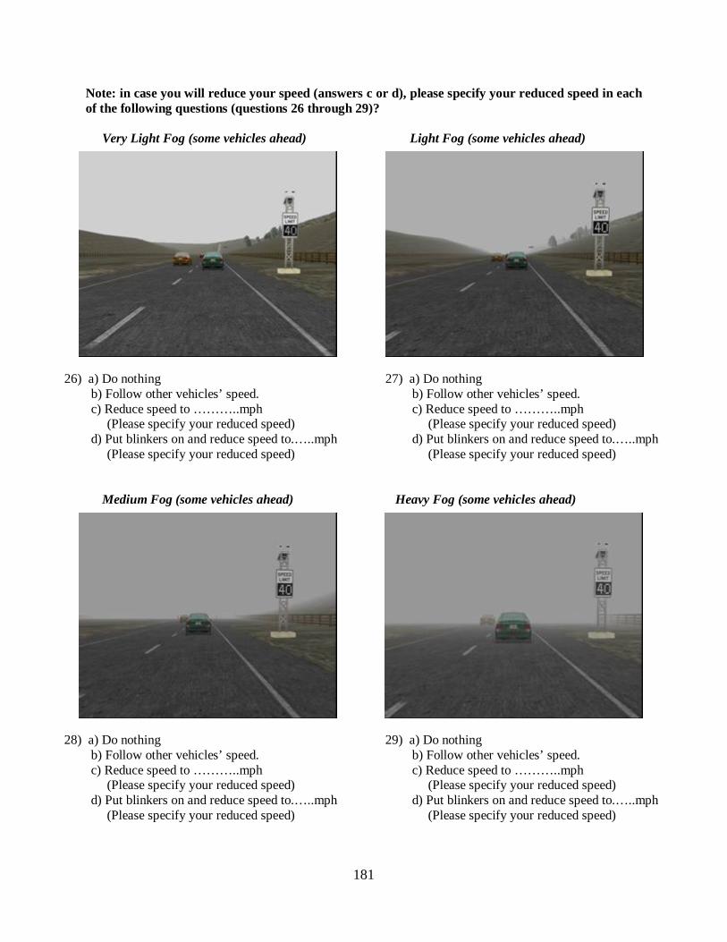
181

Note: in case you will reduce your speed (answers c or d), please specify your reduced speed in each of the following questions (questions 26 through 29)? Very Light Fog (some vehicles ahead) Light Fog (some vehicles ahead)

26) a) Do nothing 27) a) Do nothing

b) Follow other vehicles’ speed. b) Follow other vehicles’ speed. c) Reduce speed to ………..mph c) Reduce speed to ………..mph

(Please specify your reduced speed) (Please specify your reduced speed) d) Put blinkers on and reduce speed to.…..mph d) Put blinkers on and reduce speed to.…..mph (Please specify your reduced speed) (Please specify your reduced speed) Medium Fog (some vehicles ahead) Heavy Fog (some vehicles ahead)

28) a) Do nothing 29) a) Do nothing

b) Follow other vehicles’ speed. b) Follow other vehicles’ speed. c) Reduce speed to ………..mph c) Reduce speed to ………..mph

(Please specify your reduced speed) (Please specify your reduced speed) d) Put blinkers on and reduce speed to.…..mph d) Put blinkers on and reduce speed to.…..mph (Please specify your reduced speed) (Please specify your reduced speed)

182

30) Suppose you encounter a sudden reduction in visibility due to fog, smoke, or heavy rain while you are driving on a freeway/expressway (as shown in the following pictures), which of the following best describe what you will do?

a) Do nothing b) Drive below speed limit. c) Drive below speed limit following the instructions of variable speed limit sign (VSL) and/or

Changeable message sign (CMS), if they are available. d) Follow other vehicles’ speed. If they reduce their speed then you will also reduce your speed

regardless of CMS and VSL warnings. e) Drive below speed limit and put blinkers on f) Abandon the journey and stop the car immediately at the right shoulder of the road

31) Suppose you encounter a sudden reduction in visibility due to fog, smoke, or heavy rain while you are

driving on a freeway/expressway, rank the following responses from 1 to 6 where 1 is the safest action that will minimize the chance of an accident and 6 is the most dangerous action that will maximize the chance of an accident?

Responses Rank

Do nothing Drive below speed limit. Drive below speed limit following the instructions of variable speed limit sign (VSL) and/or Changeable message sign (CMS), if they are available.

Follow other vehicles’ speed. If they reduce their speed then you will also reduce your speed regardless of CMS and VSL warnings.

Drive below speed limit and put blinkers on Abandon the journey and stop the car immediately at the right shoulder of the road

End of Survey Thank you for participating in the survey!

183

APPENDIX B:

SURVEY OF TWO-LANE ROADS

184

UCF and FDOT safety study Objective of the survey Researchers at the University of Central Florida (UCF) are currently working on a Florida Department of Transportation (FDOT) sponsored project intended to reduce accidents on Florida’s Highways. To help us achieve this goal, we would like to invite you to complete a survey. All answers are anonymous. There are no anticipated risks or direct benefits to you if you decide to participate. There is no penalty if you decide not to participate. You can end your participation at anytime and you do not have to answer any questions that you do not want to answer. The survey will take only about 5 minutes of your time. WOULD YOU LIKE TO PARTICIPATE IN THIS SURVEY? If yes, please begin to answer survey’s questions. ________________________________________________________________________ Are you 18 years old or older? (Yes, No) (if “NO” terminate survey) Please choose one answer only in each of the following survey’s questions Personal information: 1) What is your gender?

a) Male b) Female

2) Which of the following best describes your age (in years)? a) 18-25 b) 26-35 c) 36-50 d) 51-65 e) over 65

3) What is the highest level of education that you have completed? a) Graduate school or higher b) College degree c) Some College d) High School e) Did not graduate from high school 4) How long have you had a valid driver’s license?......................years 5) Number of traffic citations (i.e. Traffic rule violations) in the previous 3 years?............. 6) Have you ever been involved in any crash, while you were driving in fog/smoke, due to reduction in

visibility? a) Yes b) No

7) Have you ever been involved in any crash, while you were driving in heavy rain, due to reduction in visibility?

a) Yes b) No

185

Survey Questions: 8) Have you driven on any two lane roads during the last

month? a) Yes b) No

9) How often do you use two lane roads? (One way trip is considered as one time)

a) More than four times a week b) Two-four times a week c) Once a week d) Once in two weeks Two-lane road e) Once a month f) Rarely or never

A Changeable Message Sign (CMS) is an electronic traffic sign often used on roadways to provide travelers with information about special events. Such signs warn of traffic congestion, accidents, roadwork zones, and inclement weather such as fog/smoke and heavy rain. 10) Have you ever encountered CMS on a two lane road?

a)Yes b) No

CMS A Variable Speed Limit sign (VSL) is an electronically adjustable speed limit to help manage the traffic flow (vehicles) under various traffic and environmental conditions. 11) Have you ever encountered VSL on a two lane road? a) Yes

b) No

VSL 12) If you are provided with information on CMS and/or VSL that is designed to help avoid a potential

accident in case of reduced visibility due to fog/smoke on a two way-two lane road, would you agree to follow the advice provided?

a) Strongly Agree b) Agree c) Neither agree nor disagree d) Disagree e) Strongly Disagree 13) Did you encounter any reduction in visibility due to fog, smoke, or heavy rain while you were driving

on a two lane road? a) Yes b) No (if “NO” skip question 14)

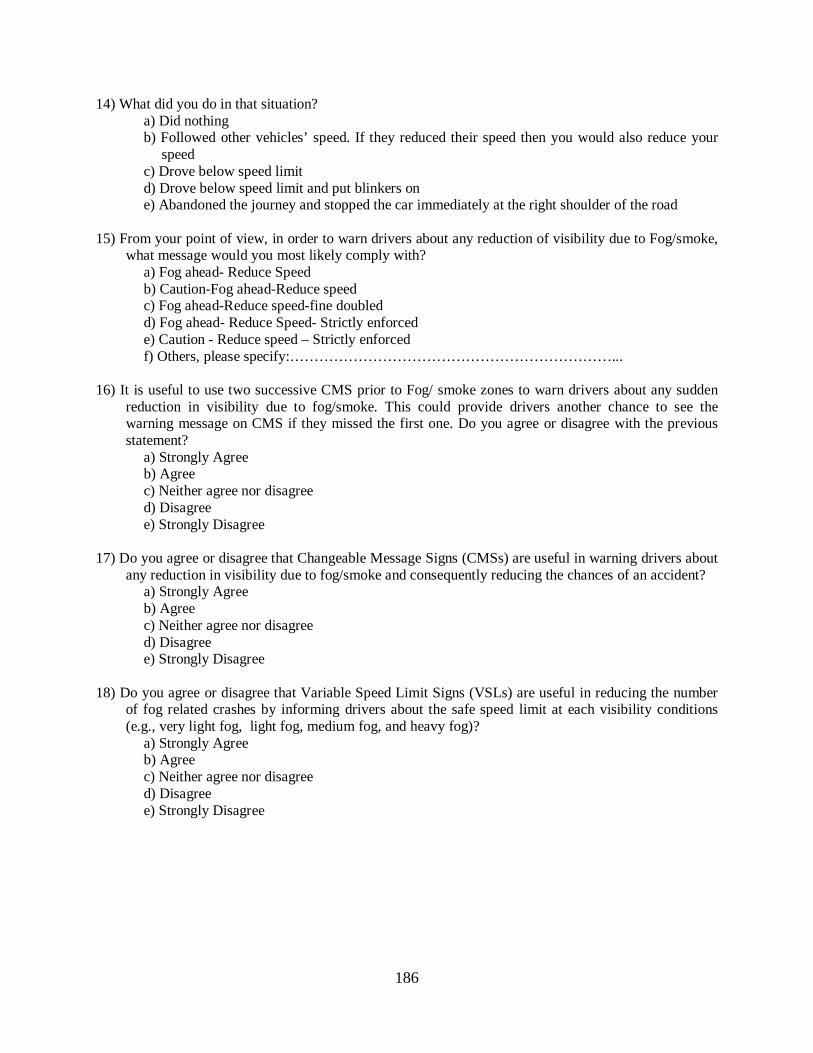
186

14) What did you do in that situation? a) Did nothing b) Followed other vehicles’ speed. If they reduced their speed then you would also reduce your

speed c) Drove below speed limit d) Drove below speed limit and put blinkers on e) Abandoned the journey and stopped the car immediately at the right shoulder of the road

15) From your point of view, in order to warn drivers about any reduction of visibility due to Fog/smoke,

what message would you most likely comply with? a) Fog ahead- Reduce Speed b) Caution-Fog ahead-Reduce speed c) Fog ahead-Reduce speed-fine doubled d) Fog ahead- Reduce Speed- Strictly enforced e) Caution - Reduce speed – Strictly enforced f) Others, please specify:…………………………………………………………...

16) It is useful to use two successive CMS prior to Fog/ smoke zones to warn drivers about any sudden

reduction in visibility due to fog/smoke. This could provide drivers another chance to see the warning message on CMS if they missed the first one. Do you agree or disagree with the previous statement?

a) Strongly Agree b) Agree c) Neither agree nor disagree d) Disagree e) Strongly Disagree 17) Do you agree or disagree that Changeable Message Signs (CMSs) are useful in warning drivers about

any reduction in visibility due to fog/smoke and consequently reducing the chances of an accident? a) Strongly Agree

b) Agree c) Neither agree nor disagree

d) Disagree e) Strongly Disagree 18) Do you agree or disagree that Variable Speed Limit Signs (VSLs) are useful in reducing the number

of fog related crashes by informing drivers about the safe speed limit at each visibility conditions (e.g., very light fog, light fog, medium fog, and heavy fog)?

a) Strongly Agree b) Agree

c) Neither agree nor disagree d) Disagree e) Strongly Disagree

187

19) From your point of view, which one of the following would improve safety during driving through fog/smoke on two lane roads?

a) Using CMS only b) Using VSL sign only

c) Using CMS and VSL signs together d) Closing the road during such adverse weather

conditions.

CMS VSL If you were driving on a two lane road at a speed of 45 mile/hour (mph), and you encounter a CMS advising you to reduce your speed because of reduction in visibility due to Fog/smoke in order to reduce the chances of an accident. What would you do in each of the following cases? No car leading ahead car leading ahead

20) a) Do nothing 21) a) Do nothing

b) Reduce speed immediately b) Reduce speed immediately c) Reduce speed after some time c) Reduce speed after some time

d) Reduce speed and put blinkers on d) Follow other vehicles’ speed regardless of CMS warning e) Reduce speed and put blinkers on

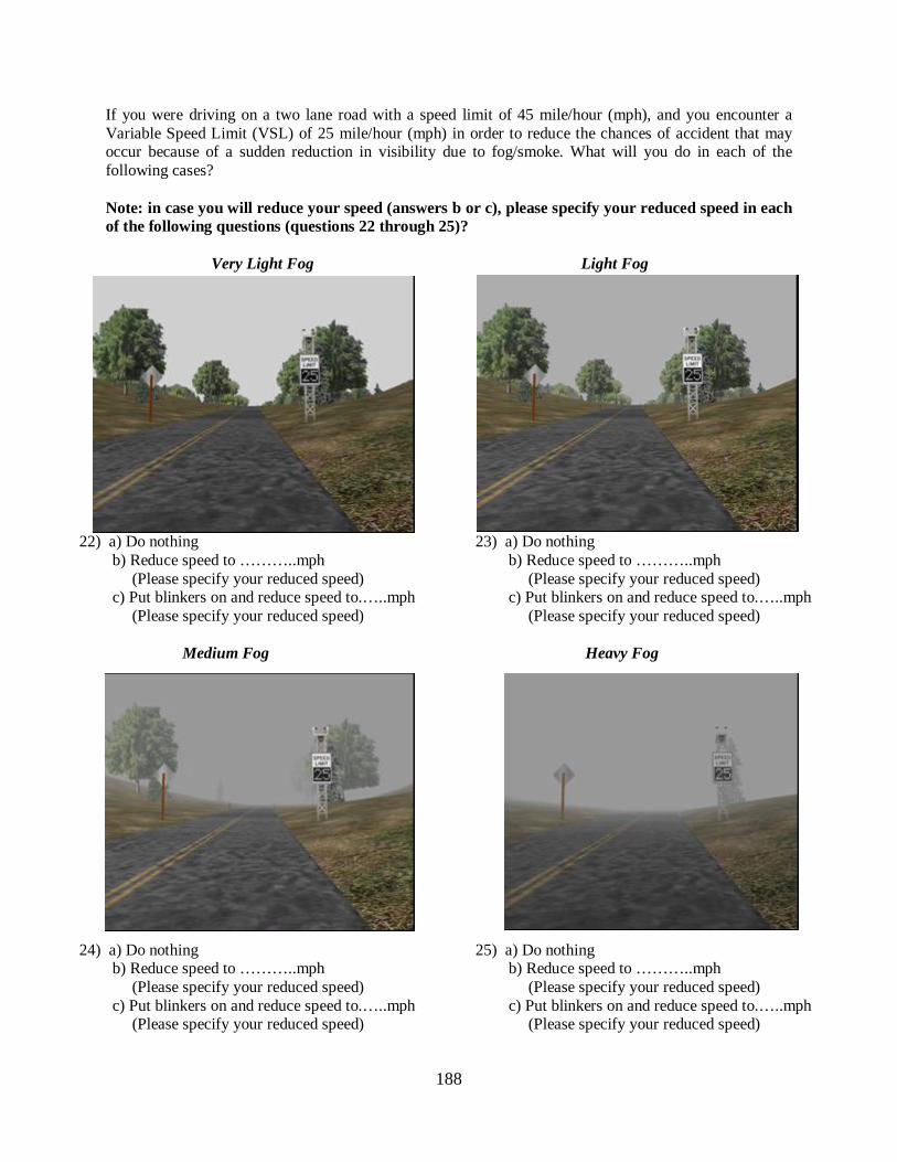
188

If you were driving on a two lane road with a speed limit of 45 mile/hour (mph), and you encounter a Variable Speed Limit (VSL) of 25 mile/hour (mph) in order to reduce the chances of accident that may occur because of a sudden reduction in visibility due to fog/smoke. What will you do in each of the following cases? Note: in case you will reduce your speed (answers b or c), please specify your reduced speed in each of the following questions (questions 22 through 25)? Very Light Fog Light Fog

22) a) Do nothing 23) a) Do nothing b) Reduce speed to ………..mph b) Reduce speed to ………..mph

(Please specify your reduced speed) (Please specify your reduced speed) c) Put blinkers on and reduce speed to.…..mph c) Put blinkers on and reduce speed to.…..mph (Please specify your reduced speed) (Please specify your reduced speed) Medium Fog Heavy Fog

24) a) Do nothing 25) a) Do nothing b) Reduce speed to ………..mph b) Reduce speed to ………..mph

(Please specify your reduced speed) (Please specify your reduced speed) c) Put blinkers on and reduce speed to.…..mph c) Put blinkers on and reduce speed to.…..mph (Please specify your reduced speed) (Please specify your reduced speed)

189

Note: in case you will reduce your speed (answers c or d), please specify your reduced speed in each of the following questions (questions 26 through 29)?

Very Light Fog (some vehicles ahead) Light Fog (some vehicles ahead)

26) a) Do nothing 27) a) Do nothing b) Follow other vehicles’ speed. b) Follow other vehicles’ speed. c) Reduce speed to ………..mph c) Reduce speed to ………..mph

(Please specify your reduced speed) (Please specify your reduced speed) d) Put blinkers on and reduce speed to.…..mph d) Put blinkers on and reduce speed to.…..mph (Please specify your reduced speed) (Please specify your reduced speed) Medium Fog (some vehicles ahead) Heavy Fog (some vehicles ahead)

28) a) Do nothing 29) a) Do nothing b) Follow other vehicles’ speed. b) Follow other vehicles’ speed. c) Reduce speed to ………..mph c) Reduce speed to ………..mph

(Please specify your reduced speed) (Please specify your reduced speed) d) Put blinkers on and reduce speed to.…..mph d) Put blinkers on and reduce speed to.…..mph (Please specify your reduced speed) (Please specify your reduced speed)

190

30) Suppose you encounter a sudden reduction in visibility due to fog, smoke, or heavy rain while you are driving on a two lane road (as shown in the following pictures), which of the following best describe what you will do?

a) Do nothing b) Drive below speed limit. c) Drive below speed limit following the instructions of variable speed limit sign (VSL) and/or

Changeable message sign (CMS), if they are available. d) Follow other vehicles’ speed. If they reduce their speed then you will also reduce your speed

regardless of CMS and VSL warnings. e) Drive below speed limit and put blinkers on f) Abandon the journey and stop the car immediately at the right shoulder of the road

31) Suppose you encounter a sudden reduction in visibility due to fog, smoke, or heavy rain while you are

driving on a two lane road, rank the following responses from 1 to 6 where 1 is the safest action that will minimize the chance of an accident and 6 is the most dangerous action that will maximize the chance of an accident?

Responses Rank

Do nothing Drive below speed limit. Drive below speed limit following the instructions of variable speed limit sign (VSL) and/or Changeable message sign (CMS), if they are available.

Follow other vehicles’ speed. If they reduce their speed then you will also reduce your speed regardless of CMS and VSL warnings.

Drive below speed limit and put blinkers on Abandon the journey and stop the car immediately at the right shoulder of the road

End of Survey Thank you for participating in the survey!

191

APPENDIX C:

APPROVAL OF EXEMPT HUMAN RESEARCH FROM IRB

192

193

LIST OF REFERENCES

1. Abdel-Aty, M., Vaughn, K., Kitamura, R., Jovanis, P., and Mannering, F. Models of

Commuters' Information Use and Route Choice: Initial results Based on a Southern

California Commuter Route Choice Survey, Journal of the Transportation Research Board,

Vol. 1453, pp. 46-55, 1994.

2. Abdel-Aty, M. and Abdelwahab, H. Toll Road Origin-Destination Travel Survey: Internet

and Mail-back Response Analysis and the Implications for Future Surveys. Journal of the

Transportation Research Board, Vol. 1768, pp. 61-70, 2001.

3. Abdel-Aty, M., Uddin, N., Abdalla, F., Pande, A., and Hsia, L. Predicting freeway crashes

based on loop detector data using matched case–control logistic regression. Transportation

Research Record. Vol. 1897, pp. 88–95, 2004.

4. Abdel-Aty, M., and A. Pande. Identifying crash propensity using specific traffic speed

conditions. Journal of Safety Research. Vol. 36, pp. 97–108, 2005.

5. Abdel-Aty, M., Pande, A., Das, A., and Knibbe, W. Assessing safety on Dutch freeways

with data from infrastructure-based intelligent transportation systems. Transportation

Research Record. Vol. 2083, pp. 153-161, 2008.

6. Acker, V. and Witlox, F. Car Ownership as a Mediating Variable in Car Travel Behaviour

Research using a Structural Equation Modeling Approach to identify its Dual Relationship.

Journal of Transport Geography, Vol. (18), pp. 65-74, 2010.

7. Agresti, A. Categorical data analysis, second edition, 2002.

8. Al-Deek, H. The Impact of Real-Time and Predictive Traffic Information on Travelers’

Behavior in the I-4 Corridor. Final report submitted to FDOT, 2003.

194

9. Al-Ghamdi, A., Experimental Evaluation of Fog Warning System, Transportation Research

Board, TRB Annual Meeting CD-ROM, Paper no. 002136, 2004.

10. Anderson, J.C. and Gerbing, D.W. Structural equation modeling in practice: A review and

recommendation two-step approach. Psychological Bulletin, Vol. 103, pp. 411-423, 1988.

11. Andersen, J., Kang, J., and Ni, R. The Effects of Reduced Visibility from Fog on Car

Following Performance, Transportation Research Board, TRB Annual Meeting CD-ROM,

2008.

12. Andrey, J., Mills, B., and Vandermolen, J. A Temporal Analysis of Weather-related

Collision Risk for Ottawa, Canada: 1990-1998, Transportation Research Board, TRB Paper

03-3488, 2003.

13. Ashford, R., and Sowden, R. Multivariate probit analysis, Biometrics, Vol. 26, pp. 535-

546, 1970.

14. Benson, B. Motorist Attitudes about Content of Variable-Message Signs. Transportation

Research Record: Journal of the Transportation Research Board, Vol. 1550, pp. 48-57,

1996.

15. Bentler, P.M. and Bonett, D.G. Significance tests and goodness of fit in the analysis of

covariance structures. Psychological Bulletin, Vol. (88), pp. 588-606, 1980.

16. Berger, J. Statistical Decision Theory and Bayesian Analysis, second edition, 1985.

17. Braham, P., Andreone, L., Zhang, X., and Vache, M. The “DRAWN” Driver Vision

Support System: ITS Potential Impact on Driving Behavior and Road Safety, in Conditions

of Reduced Visibility. In Proc., Seminar J, European Transport Conference, Cambridge,

England, 2000.

195

18. Breiman, L. Some infinity theory for predictor ensembles. Technical Report 579, Statistics

Dept. University of California Barkley, 2000.

19. Brodsky, H. and Hakkert, A. Risk of a Road Accident in Rainy Weather. Accident Analysis

and Prevention, Vol. 20, pp. 161-176, 1988.

20. Bross, I. How to use ridit analysis. Biometrics, Vol. 14, pp. 18-38, 1958.

21. Broughton, K., Switzer, F., and Scott, D. Car following decisions under three visibility

conditions and two speeds tested with a driving simulator, Accident Analysis and

Prevention Part 39, PP. 106–116, 2007.

22. Brow, B., and Baass, K., Seasonal Variation in Frequencies and Rates of Highway

Accidents as a Function of Severity. Transportation Research Record, Vol. 1581, pp. 59-

65, 1997.

23. Carlsson, F., Daruvala, D. and Jaldell H. Preferences for lives, injuries, and age: A stated

preference survey. Accident Analysis and Prevention, Vol. (42), pp. 1814–1821, 2010.

24. Center for Urban Transportation Research (CUTR), “Evaluation of Motorist Warning

Systems for Fog-Related Incidents in the Tampa Bay Area,” University of South Florida, p.

25, June 1997, http://www.cutr.eng.usf.edu/research/fog.pdf.

25. Chatterjee, K., Hounsell, N., Firmin, P. and Bonsall P. Driver response to variable message

sign information in London. Journal of the Transportation Research Board, Vol. 10, pp.

149-169, 2002.

26. Chin, S., et al., Temporary Losses of Highway Capacity and Impacts on Performance,

ORNL/TM-2002/3, Oak Ridge National Laboratory, 2002.

27. Choo, S., and Mokhtarian, P. How do People Respond to Congestion Mitigation Policies?

A Multivariate Probit Model of the Individual Consideration of Three Travel-Related

196

Strategy Bundles. Journal of the Transportation Research record, Vol. 35, pp. 145-163,

2008.

28. Cooper, B., Sawyer, H. Assessment of M25 Automatic Fog-Warning System - Final

Report, Transport Research Laboratory, Old Wokingham Road, Crowthorne, Berkshire,

Rg11 6au, United Kingdom, TRL Project Report, Issue Number: PR 16, IRRD Document

Number: 858269, 1993.

29. Correia, G. and Viegas, J. Carpooling and carpool clubs: Clarifying concepts and assessing

value enhancement possibilities through a Stated Preference web survey in Lisbon,

Portugal. Transportation Research Part A, Vol. (45), pp. 81–90, 2011.

30. Cummings, G., Harrison, W., and Rutstrim, E. Homegrown Values and Hypothetical

Surveys: Is the Dichotomous Choice Approach Incentive-Compatible? American

Economic Review, Vol. 85 (1), pp. 260-266, 1995.

31. Dahlinger, D. and McCombs, B. Fog Warning System Provides a Safety Net for Motorist,

Public Works, December 1995.

32. Dahlinger, D. “Tennessee Fog Detection and Warning System,” Public Works, presented at

the Southern Rural Transportation Workshop, May 2001.

33. Das, A., Pande, A., Abdel-Aty, M., and Santos, J. Characteristics of Urban Arterial Crashes

Relative to Proximity to Intersections and Injury Severity. Journal of the Transportation

Research Board, Vol. 2083, pp. 137-144, 2008.

34. Dion, F. and Rakha, H. Estimating dynamic roadway travel times using automatic vehicle

identification data for low sampling rates, Transportation Research Part B 40, 745–766,

2006.

197

35. Dion, P. Interpreting Structural Equation Modeling. Journal of Business Ethics. Vol. 83,

pp. 365–368, 2008.

36. Dudek, C. and Ullman, G. Flashing Messages, Flashing Lines, and Alternating One Line on

Changeable Message Signs. Transportation Research Record, Vol. 1803, p.p. 94-101, 2002.

37. Dudek, C., Schrock, S., and Ullman, G., Impacts of Using Dynamic Features to Display

Messages on Changeable Message Signs, U.S Department of Transportation, Federal

Highway Administration, Publication No. FHWA-HOP-05-069, August 2005.

38. Dudek, C., Schrock, S., Ullman, G. and Chrysler, S. Flashing Message Features on

Changeable Message Signs. Transportation Research Record, Vol. 1959, p.p. 122-129,

2006.

39. Dudek, E., and Steven, S. Flashing Message Features on Changeable Message Signs,

Transportation Research Board of the National Academies, volume 1959, 2006.

40. Edwards, J., Weather-related road accidents in England and Wales: a spatial analysis,

Journal of Transport Geography Vol. 4, No. 3, pp. 201-212, 1996.

41. Edwards, J. Speed adjustment of motorway commuter traffic to inclement weather. Journal

of the Transportation Research Board, Vol. 2, pp. 1-14, 1999.

42. Eissenberg, D. The Mixed Effects of Precipitation on Traffic Crashes. Accident Analysis

and Prevention, Vol., 36, pp. 637 – 647, 2004.

43. Emmerink, R., Nijkamp, P., Rietveld, P., and Ommeren, J. Variable Message Signs and

Radio Traffic Information: An Integrated Empirical Analysis of Drivers’ Route Choice

Behavior” Transportation Research Part A. Vol. 30, No. 2, pp. 135-153, 1996.

44. Fleiss, J. Statistical methods for Rates and Proportions. John Wiley & Sons, 2nd Edition,

New York, 1981.

198

45. Gelfand, E. and Smith, M. Sampling-based approaches to calculating marginal densities.

Journal of American Statistics Association, Vol. (85), pp. 398-409, 1990.

46. Gibbons, R., Wilcox-Gök, V. Health service utilization and insurance coverage: A

multivariate probit approach. Journal of the American Statistical Association, Vol. 93

(441), pp. 63-72, 1998.

47. Gimmestad, G., Daley, W., Carey, R., Moses, M., and Usher, C. Georgia Automated

Adverse Visibility Warning and Control System, GDOT Research Project No. 9304, Final

Report, September 2004.

48. Goldstein, H. Multilevel Statistical Models, third ed. Hodder Arnold, London, 2003.

49. Golob, T. and Recker, W. Relationships among urban freeway accidents, traffic flow,

weather and lighting conditions. California PATH program, institute of transportation

studies, Berkeley, ISSN 1055-1417, UCB-ITS-PWP-19, 2001.

50. Golob, T., and Recker, W. A Method for Relating Type of Crash to Traffic Flow

Characteristics on Urban Freeways” Presented at the Annual Meeting of the Transportation

Research Board, Washington, DC, January 2003.

51. Golob, T., Recker, W., and Alvarez, V. Freeway safety as a function of traffic flow.

Accident analysis and prevention, Vol. 36, 933-946, 2004.

52. Goodwin, L. Best Practices for Road Weather Management, Version 2.0, report no.

FHWA-OP-03-081, May 2003.

53. Gordon, R. Traffic Control Systems Handbook, prepared by Dunn Engineering Associates,

Publication No. FHWA-SA-95-032, FHWA, U.S. DOT, p. 4-18, February 1996.

54. Greene, W. Econometric Analysis. Pearson Education, Inc., 5th Edition, 2003.

199

55. Grimm, R., Behrens, T., Marker, M. and H. Elsenbeer. Soil organic carbon concentrations

and stocks on Barro Colorado Island. Digital soil mapping using Random Forests analysis.

Geoderma, Vol. 146, No. 1-2, pp. 102-113, 2008.

56. Han, L., Chin, S., and Hwang, H. Estimating Adverse Weather Impacts on Major US

Highway Network, Transportation Research Board, Annual Meeting CD-ROM, Paper No.

002155, 2003.

57. Hanbali, R. Economic Impact of Winter Road Maintenance on Road Users. Transportation

Research Record, Vol. 1442, pp. 151-161, 1994.

58. Harris, P., and Konheim, C. Public Interest in, and Willingness to Pay for, Enhanced

Traveler Information as Provided by IVHS in the New York Metropolitan Area.

Proceedings of the 5th Annual Meeting of ITS America, 1995.

59. Haselkorn, M., Spyridakis, J., Conquest, L., and Barfield, W. Surveying Commuter

Behavior as a Basis for Designing Motorist Information Systems. Proceedings of the

Conference on Vehicle Navigation and Information Systems (VNIS), pp. 93-100, 1989.

60. Hassan, H., Abdel-Aty, M. and Oloufa, A. The Effect of Warning Messages and Variable

Speeds in Different Visibility Conditions, Transportation Research Board, 90th Annual

Meeting, paper no. 11-0354, 2011.

61. Hassan, H. and Abdel-Aty, M. Exploring Visibility Related Crashes on Freeways based On

Real-time Traffic Flow Data, Transportation Research Board, 90th Annual Meeting,

Washington D.C., paper no. 11-0920, 2011.

62. Hatcher, L. A step-by-step Approach to Using SAS for Factor Analysis and Structural

Equation Modeling. Cary, NC: SAS Institute Inc, 1994.

200

63. Ho, T. The random subspace method for constructing decision forests. IEEE Trans. on

Pattern Analysis and Machine Intelligence, Vol. 20(8), pp. 832–844, 1998.

64. Hogema, J., and Horst, R. Evaluation of A16 Motorway Fog-Signaling System with

Respect to Driving Behavior. Journal of Transportation Research Board, Vol. 1573, pp. 63-

67, 1997.

65. Hoogen, V., and Smulders, S. Control by variable speed signs: results of the Dutch

experiment. Institute of Electrical Engineers IEE, pp. 145-149, 1994.

66. Huang H., Chin H., and Haque M. Severity of driver injury and vehicle damage in traffic

crashes at intersections: Bayesian hierarchical analysis. Accident Analysis & Prevention,

Vol. 40(1), pp. 45-54, 2008.

67. Huang, H., Abdel-Aty, M., Ekram, A., Oloufa, A., Chen, Y., and R. Morrow. Fog and

Smoke Related Crashes in Florida: Identifying Crash Characteristics, Spatial Distribution

and Injury Severity, presented at the 89th Annual Meeting of the Transportation Research

Board, 2010.

68. Ikeda A., Katou T., Kinoshita M. and Aihara M. Study of driver characteristics using

driving simulator considerations on difference in accident avoidance performance due to

age. JSAE Review Vol. 23, pp 219–222, 2002.

69. Iragüen, P. and Ortúzar, J. Willingness-to-pay for reducing fatal accident risk in urban

areas: an Internet-based Web page stated preference survey. Accident Analysis and

Prevention, Vol. 36, pp. 513–524, 2004.

70. James, L.R., Mulaik, S.A. and Brett, J.M. Causal Analysis. Beverly Hills: Sage, 1982.

201

71. Johannesson, M., Liljas, B. and Johansson, P. An Experimental Comparison of

Dichotomous Choice Contingent Valuation Questions and Real Purchase Decisions.

Applied Economics, Vol. 30 (5), pp. 643-647, 1998.

72. Junyi, Z., Akimasa, F. and Soe, T. Capturing Travelers’ Stated Mode Choice Preferences

Under Influence of Income in Yangon City, Myanmar. Journal of Transportation System

and Information Technology, Vol. (8), Issue (4), 2008.

73. Khattak, A., Polydoropoulou, A., and Ben-Akiva, M. Modeling revealed and stated pre-trip

travel response to ATIS. Transportation Research Record, Vol. 1537, pp. 46-54, 1996.

74. Khattak, A., Kantor, P., and Council, F. Role of Adverse Weather in Key Crash Types on

Limited Access Roadway – Implications for Advanced Weather System, Transportation

Research Record, Vol. 1621, pp. 10-19, 1998.

75. Khattak, A., Knapp, K., Giese, K., and Smithson, L. Safety Implications of Snowstorms on

Interstate Highways. Presented at the Annual Meeting of the Transportation Research

Board, Washington, D.C., 2000.

76. Kilpelainen, M., and Summala, H. Effects of weather and weather forecasts on driver

behavior. Transportation Research Part F, pp. 288–299, 2007.

77. Kim, K., Pant, P. and Yamashita, E. Measuring the Influence of Accessibility on Accident

Severity with Structural Equation Modeling. TRB Annual Meeting CD-ROM, paper no.

11-2663, 2011.

78. Knapp, K. Investigation of Volume, Safety, and Vehicle Speeds during Winter Storm

Events. Ninth AASHTO/TRB Maintenance Management Conference, Juneau, Alaska, pp.

57-64, August, 2000.

202

79. Kuhn, S., Egert, B., Neumann, S. and C. Steinbeck. Building blocks for automated

elucidation of metabolites: Machine learning methods for NMR prediction. BMC

Bioinformatics, Vol. 9 (400), 2008.

80. Kyte, M., Shannon, P., and Kitchener, F. Idaho Storm Warning System Operational Test,

Final Report, ITD No. IVH9316 (601), NIATT Report No. N00-04, December 2000.

81. Lai, C. Effects of color scheme and message lines of variable message signs on driver

performance, Accident Analysis and Prevention, Vol. 42, pp. 1003–1008, 2010.

82. Lai K. and Wong W. SP Approach toward Driver Comprehension of Message Formats on

VMS. Journal of Transportation Engineering, Vol. 126, No. 3, 2000.

83. Lai, C., and Yen K. Sedan drivers’ attention and response to variable message signs on

freeway in Taiwan. Presented at the 4th International Conference on Traffic and

Transportation Psychology, Nottingham, UK, 2004.

84. Lansink, A., Berg, M., and Huirne, R. Analysis of strategic planning of Dutch pig farmers

using a multivariate probit model. Agricultural Systems, Vol. 78, pp. 73-84, 2003.

85. Lee, C., Saccomanno, F., and Hellinga, B. Analysis of crash precursors on instrumented

freeways. Transportation Research Record. Vol. 1784, pp 1–8, 2002.

86. Lee, C., Saccomanno, F., and Hellinga, B. Real-time crash prediction model for the

application to crash prevention in freeway traffic. Transportation Research Record. Vol.

1840, pp. 68–77, 2003.

87. Lee, J., Chung, J., and Son, B. Analysis of Traffic Accident for Korean Highway Using

Structural Equation Models. Accident Analysis and Prevention (40), pp. 1955-1963, 2008.

203

88. Liang, W., Kitchener, F., Kyte, M., and Shannon, P. the Effect of Environmental Factors on

Driver Speed: A Case Study, presented at Transportation Research Board, 77th Annual

Meeting, January, 1998.

89. Loomis, J. An Investigation into the Reliability of Intended Visitation Behavior.

Environmental and Resource Economics, Vol. 3 (2), pp. 183-191, 1993.

90. Lu, B., and Song, X. Local influence analysis of multivariate probit latent variable models.

Journal of Multivariate Analysis, Vol. 97, pp. 1783-1798, 2006.

91. Luoma, J., Rama, P., Penttinen, M., and Anttila, V. Effects of variable message signs for

slippery road conditions on reported driver behavior, Transportation Research Part F, Vol.

3, pp.75-84, 2000.

92. Lynn, C., Schreiner, C., and Campbell, R. Reducing Fog-Related Crashes on the Afton and

Fancy Gap Mountain Sections of I-64 and I-77 in Virginia, Report FHWA/VTRC 03-CR2,

Virginia Transportation Research Center, Charlottesville, 2002.

93. Ma, M., Yan, X., Huang, H. and Abdel-Aty, M. Safety of Public Transportation

Occupational Drivers. Transportation Research Record, No. 2145, pp. 72-79, 2010.

94. Madanat, S., and P. Liu. A prototype system for real-time incident likelihood prediction.

IDEA project final report (ITS-2), Transportation Research Board, National Research

Council, Washington, D.C., 1995.

95. Mahmassani, H., Huynh, N., Srinivasan, K. and Kraan, M. Tripmaker choice behavior for

shopping trips under real-time information: model formulation and results of stated-

preference internet-based interactive experiments. Journal of Retailing and Consumer

Services, Vol. 10, pp. 311–321, 2003.

204

96. Martínez, L., Silva, J., and Viegas, J. Assessment of Residential Location Satisfaction in

the Lisbon Metropolitan Area. TRB Annual Meeting CD-ROM, 2010.

97. McBride, J., Benlangie, M., Kennedy, W., McCornkie, F., Steward, R.M., Sy, C., and

Thuet, J., Economic Impacts of Highway Snow and Ice Control. National Pool Fund Study

Report FHWA-RD-77-95, Federal Highway Administration, U.S. Department of

Transportation, 1977.

98. MacCarley, A. Evaluation of Caltrans District 10 Automated Warning System, Cal Poly

Transportation Electronics Laboratory, year one progress report, June 10, 1998.

99. MacCarley, A. Evaluation of Caltrans District 10 Automated Warning System, Year Two

Progress Report, California PATH Research Report, UCB-ITS-PRR-99-28, August 1999.

100. MacCarley, C., Ackles, C., and Watts, T. A Study of the Response of Highway Traffic to

Dynamic Fog Warning and Speed Advisory Messages. TRB Annual Meeting CD-ROM,

paper no. 06-3086, 2006.

101. Maze, T., Agarwal, M., and Souleyrette, R. Impact of Weather on Urban Freeway Traffic

Flow Characteristics and Facility Capacity, Final Technical Report, Aurora project ,

Center for Transportation Research and Education, Iowa State University, August 2005.

102. Maze, T., Agarwal, M., and Burchett, G. Whether Weather Matters To Traffic Demand,

Traffic Safety, and Traffic Operations and Flow, TRB Annual Meeting CD-ROM, paper

no. 06-0808, 2006.

103. Meng, C. and Schmidt, P. On the cost of partial observability in the bivariate probit model.

International Economic Review, Vol. 26, pp. 71-76, 1985.

205

104. Mitchell, G., Schattler, K., and Datta, T. Use of a Driving Simulator for Evaluation of

Safety Measures in Highway Work Zones, Presented at the 84th Annual Meeting of the

Transportation Research Board, Washington, D.C, 2005.

105. Mohanty, M. A bivariate probit approach to the determination of employment: a study of

teen employment differentials in Los Angeles County. Applied Economics, Vol. 34, pp.

143-156, 2002.

106. Nachimas, F. and Nachmias, D. Research Methods in the Social Sciences. St. Martin’s

Press, 5th Edition, New York, 1996.

107. Ng, L., Mannering, F. Statistical Analysis of the Impact of Traveler Advisory Systems on

Driving Behavior” Presented at the 77th Annual Meeting of the Transportation Research

Board, 1998.

108. Nixon, W. The Potential of Friction as a Tool for Winter Maintenance. Iowa Institute of

Hydraulic Research Report No. 392, College of Engineering, the University of Iowa, Iowa

City, Iowa, February, 1998.

109. Norrman, J., Eriksson, M., and Lindqvist, S. “Relationship between Road Slipperiness,

Traffic Accident Risk and Winter Road Maintenance Activity,” Climate Research, Vol. 15,

pp. 185–193, September, 2000.

110. Nunnally, J. (1978). Psychometric Theory, 2nd edition. McGraw-Hill, New York.

111. Oh, C., Oh, J., Ritchie, S., and Change M. Real time estimation of freeway accident

likelihood. Presented at the 80th annual meeting of Transportation Research Board, 2001.

112. Pande, A., and Abdel-Aty, M. Assessment of freeway traffic parameters leading to lane-

change related collisions. Accident analysis and prevention. Vol. 38, pp. 936-948, 2006.

206

113. Peeta S. and Ramos J. Driver Response to Variable Message Signs-Based Traffic

Information. IEE Proceedings online no. 20055012, 2006.

114. Perrin J. Effects of Variable Speed Limit Signs on Driver Behavior during Inclement

Weather,” presented at Institute of Transportation Engineers (ITE) Annual Meeting,

August 2000.

115. Perrin, J., Martin, P., and Coleman B. Testing the Adverse Visibility Information System

Evaluation (ADVISE) – Safer Driving in Fog. Presented at Annual meeting of the

Transportation Research Board, TRB, Paper no. 02-3140, 2002.

116. Perry, A., and Symons, L. Highway Metrology. University of Wales, Swansea, Wales,

United Kingdom, 1991.

117. Pietrzyk, M. Getting clear in fog-related crashes in Tampa Bay. Institute of Transportation

Engineers. ITE Journal, 26-31, Feb 2000.

118. Pisano, P., and Goodwin, L. Research Needs for Weather-Responsive Traffic Management,

Transportation Research Board, TRB Annual meeting, paper no. 002717, 2004.

119. Rama, P., Kulmala, R. Effects of variable message signs for slippery road conditions on

driving speed and headways, Transportation Research Part F, Vol. 3, pp 85-94, 2000.

120. Rakauskas, M., Ward, N., Boer, E., Bernat, E., Cadwallader, M., and Patrick, C. Combined

effects of alcohol and distraction on driving performance. Accident Analysis and

Prevention, Vol. 40, pp 1742–1749, 2008.

121. Rakha, H. and Zhang, W. Estimating Traffic Stream Space Mean Speed and Reliability

from Dual- and Single-Loop Detectors. Transportation Research Record, 1925, 38-47,

2005.

122. Rao, J.N.K. Small Area Estimation. Wiley, New York, 2003.

207

123. Reimer, B., D’Ambrosio, L. and Coughlin J. Secondary analysis of time of day on

simulated driving performance. Journal of Safety Research, Vol. 38, pp. 563–570, 2007.

124. Rentziou, A., Milioti, C., Gkritza, K., and Karlaftis M. Urban Road Pricing: Modeling

Public Acceptability. Presented at the annual meeting of Transportation Research Board,

2010.

125. Rockwell Transportation Systems, Anaheim, CA. Adverse Visibility Information System

Evaluation (ADVISE), System Design Document, Prepared for Utah Department of

Transportation, January 14, 1997.

126. Sabra, Wang & Associates, I-68 fog detection system planning report, 2003.

127. SAS Institute Inc. SAS/STAT 9.2 User’s Guide, Second Edition. Cary, NC, 2009.

[http://support.sas.com/documentation/cdl/en/statug/63033/HTML/default/viewer.htm#intr

obayes_toc.htm].

128. Savenhed, H. Relationship between Winter Road Maintenance and Road Safety. Swedish

Road and Traffic Research Institute (VTI) Sartryck, Report No. 214, 1994.

129. Scharsching, H. Nowcasting Road Conditions: A System for Improving Traffic Safety in

winter time. Conference proceedings, Swedish Road and Traffic Research Institute (VTI)

Sartryck, pp. 142-153, 1996.

130. Schreiner, C. State of the Practice and Review of the Literature: Survey of Fog

Countermeasures Planned or in Use by Other States, Virginia Tech Research Council,

October 2000.

131. Shah, V., et al, Analysis of Weather Impacts on Traffic Flow in Metropolitan Washington

DC, Mitretek Systems, presented at the Intelligent Transportation Systems of America

Annual Meeting, May 2003.

208

132. Shankar, V., Mannering, F., and Barfield, W. Effect of Roadway Geometrics and

Environmental Factors on Rural Freeway Accident Frequencies, Accident Analysis and

Prevention, Vol. 27, pp. 371-389, 1995.

133. Singh, S. Driver Attributes and Rear-end Crash Involvement Propensity. NHTSA

Technical Report, DOT HS 809 540, 2003. [http://www-nrd.nhtsa.dot.gov/Pubs/809-

540.pdf].

134. Smith, A. Illustration of Bayesian inference in normal data models using Gibbs sampling.

Journal of American Statistics. Association, Vol. 85 pp.972-985, 1990.

135. Spector, P.E. Summated rating scale construction: An introduction. Newbury Park, CA:

Sage, 1992.

136. Spiegelhalter, D.J., Best, N.G., Carlin, B.P., Linde, V.D. Bayesian measures of model

complexity and fit. Journal of the Royal Statistical Society B, 64 (4), 583–616, 2003.

137. Tilahun, N., Levinson, D. and Krizek, K. Trails, lanes, or traffic: Valuing bicycle facilities

with an adaptive stated preference survey. Transportation Research Part A, Vol. 41, pp.

287–301, 2007.

138. Tennessee ITS State Status Report, “Fog Project on I-75 between Chattanooga and

Knoxville,” October 2000, www.its.dot.gov/staterpt/tn.htm.

139. Transit Cooperative Research Program (TCRP). Web-based survey techniques, a synthesis

of transit practice. TRB Annual Meeting CD-ROM, Washington D.C., 2006.

140. Ullman, B., Ullman, G. and Dudek, C. Driver Understanding of Messages Displayed on

Sequential Portable Changeable Message Signs in Work Zones. TRB Annual Meeting CD-

ROM, paper no. 07-1487, 2007.

209

141. U.S. Department of Transportation (DOT), Federal Highway Administration (FHWA).

How do weather events impact roads?, 2009.

http://ops.fhwa.dot.gov/weather/q1_roadimpact.htm.

142. U.S. DOT, “Mobile, Alabama Fog Detection System,” Intelligent Transportation Systems

(ITS) Projects Book, FHWA, ITS Joint Program Office, 2001.

143. Wang, J., and Cao, Y. Assessing Message Display Formats of Portable Variable Message

Signs. Transportation Research Record, Vol. 1937, pp. 113-119, 2005.

144. Wardman, M., Bonsall, P. and Shires, J. Driver Response to Variable Message Signs: A

Stated Preference Investigation. Transportation Research-C, Vol. 5, No. 6, pp. 389-405,

1997.

145. Wardrop J.G. Some Theoretical Aspects of Road Traffic Research, Proceedings of the

Institute of Civil Engineers, 1-2, 325-378, 1952.

146. West, R., French, D., Kemp, R. and Lander, J. Direct Observation of Driving, Self Reports

of Driving Behavior and Accident Involvement. Ergonomics, Vol. 36, No. 5, pp. 557-567,

1993.

147. Yannis, G., Kanellopoulou, A., Aggeloussi, K. and Tsamboulas, D. Modeling driver

choices towards accident risk reduction. Safety Science, Vol. (43), pp. 173–186, 2005.

148. Young, G., Valdez, E., and Kohn, R. Multivariate probit models for conditional claim-

types. Mathematics and Economics, Vol. 44, pp. 214-228, 2009.

149. Zhou, M. and V. Sisiopiku. Relationship between volume-to-capacity ratios and accident

rates. Transportation Research Record, Vol. 1581, pp. 47-52, 1997.

210

150. Zwahlen, H., and Russ, A. Evaluation of the Motoring Public’s Acceptance of a Real-Time

Travel Time Prediction System in a Freeway Construction Work Zone” Presented at the

81th Annual Meeting of the Transportation Research Board, Paper No. 02-2372, 2002.