In a World of P=BPP

Oded Goldreich

Abstract. We show that proving results such as BPP = P essentiallynecessitate the construction of suitable pseudorandom generators (i.e.,generators that suffice for such derandomization results). In particular,the main incarnation of this equivalence refers to the standard notion ofuniform derandomization and to the corresponding pseudorandom gen-erators (i.e., the standard uniform notion of “canonical derandomizers”).This equivalence bypasses the question of which hardness assumptionsare required for establishing such derandomization results, which hasreceived considerable attention in the last decade or so (starting withImpagliazzo and Wigderson [JCSS, 2001]).We also identify a natural class of search problems that can be solved bydeterministic polynomial-time reductions to BPP. This result is instru-mental to the construction of the aforementioned pseudorandom genera-tors (based on the assumption BPP = P), which is actually a reductionof the “construction problem” to BPP.

Caveat: Throughout the text, we abuse standard notation by lettingBPP,P etc denote classes of promise problems. We are aware of thepossibility that this choice may annoy some readers, but believe thatpromise problem actually provide the most adequate formulation of nat-ural decisional problems.1

Keywords: BPP, derandomization, pseudorandom generators, promiseproblems, search problems, FPTAS, randomized constructions.

An early version of this work appeared as TR10-135 of ECCC.

1 Introduction

We consider the question of whether results such as BPP = P necessitate theconstruction of suitable pseudorandom generators, and conclude that the answeris essentially positive. By suitable pseudorandom generators we mean generatorsthat, in particular, imply that BPP = P . Thus, in a sense, the pseudorandomgenerators approach to the BPP-vs-P Question is complete; that is, if the ques-tion can be resolved in the affirmative, then this answer follows from the existenceof suitable pseudorandom generators.

The foregoing equivalence bypasses the question of which hardness assump-tions are required for establishing such derandomization results (i.e., BPP = P),

1 Actually, the common restriction of general studies of feasibility to decision problemsis merely a useful methodological simplification.

102

which is a question that has received considerable attention in the last decade orso (see, e.g., [16, 14, 18]). Indeed, the current work would have been obsolete if itwere the case that the known answers were tight in the sense that the hardnessassumptions required for derandomization would suffice for the construction ofthe aforementioned pseudorandom generators.

1.1 What is meant by suitable pseudorandom generators?

The term pseudorandom generator is actually a general paradigm spanningvastly different notions that range from general-purpose pseudorandom gener-ator (a la Blum, Micali, and Yao [1, 26]) to special-purpose generators (e.g.,pairwise-independence ones [2]). The common theme is that the generators aredeterministic devices that stretch short random seeds into longer sequences thatlook random in some sense, and that their operation is relatively efficient. Thespecific incarnations of this general paradigm differ with respect to the specificformulation of the three aforementioned terms; that is, they differ with respectto the requirements regarding (1) the amount of stretching, (2) the sense inwhich the output “looks random” (i.e., the “pseudorandomness” property), and(3) the complexity of the generation (or rather the stretching) process.

Recall that general-purpose pseudorandom generators operate in (some fixed)polynomial-time while producing outputs that look random to any polynomial-time observers. Thus, the observer is more powerful (i.e., runs for more time)than the generator itself. One key observation of Nisan and Wigderson [19] is thatusing such general-purpose pseudorandom generators is an over-kill when thegoal is to derandomize complexity classes such as BPP. In the latter case (i.e., forderandomizing BPP) it suffices to have a generator that runs in exponential time(i.e., time exponential in its seed’s length), since our deterministic emulation ofthe resulting randomized algorithm is going to incur such a factor in its running-time anyhow.2 This leads to the notion of a canonical derandomizer, which foolsobservers of fixed complexity, while taking more time to produce such foolingsequences.

Indeed, the aforementioned “suitable pseudorandom generators” are (various(standard) forms of) canonical derandomizers. Our starting point is the non-uniform notion of canonical derandomizers used by Nisan and Wigderson [19],but since we aim at “completeness results” (as stated up-front), we seek uniform-complexity versions of it. Three such versions are considered in our work, andtwo are shown to be sufficient and necessary for suitable derandomizations ofBPP.

The last assertion raises the question of what is meant by a suitable de-randomization of BPP. The first observation is that any reasonable notion of acanonical derandomizer is also applicable to promise problems (as defined in [3]),

2 Recall that the resulting (randomized) algorithm uses the generator for producingthe randomness consumed by the original (randomized) algorithm, which it emulates,and that our deterministic emulation consists of invoking the resulting (randomized)algorithm on all possible random-pads.

103

and so our entire discussion refers to BPP as a class of promise problems (ratherthan a class of standard decision problems).3

The second observation is that standard uniform-complexity notions of canon-ical derandomizers would not allow to place BPP in P , because rare instancesthat are hard to find may not lead to a violation of the pseudorandomness guar-antee. The known fix, used by Impagliazzo and Wigderson in [16], is to consider“effective derandomization” in the sense that each problem Π ∈ BPP is ap-proximated by some problem Π ′ ∈ P such that it is hard to find instances inthe symmetric difference of Π and Π ′. Our main result refers to this notion(see Sections 4.2–4.3): Loosely speaking, it asserts that canonical derandomizers(of exponential stretch) exist if and only if BPP is effectively in P . We stressthat this result refers to the standard notion of uniform derandomization andto the corresponding canonical derandomizers (as in [16] and subsequent works(e.g. [23])).

We also consider a seemingly novel notion of canonical derandomizers, whichis akin to notions of auxiliary-input one-way functions and pseudorandom gen-erators considered by Vadhan [25]. Here the generator is given a target stringand the distribution that it produces need only be pseudorandom with respectto efficient (uniform) observers that are given this very string as an auxiliaryinput. We show that such canonical derandomizers (of exponential stretch) existif and only if BPP = P ; for details, see Section 4.4.

1.2 Techniques

Our starting point is the work of Goldreich and Wigderson [9], which studiedpseudorandomness with respect to (uniform) deterministic observers. In particu-lar, they show how to construct, for every polynomial p, a generator of exponen-tial stretch that works in time polynomial in its output and fools all deterministicp-time tests of the next-bit type (a la [1]). They observe that an analogous con-struction with respect to general tests (i.e., deterministic p-time distinguishers)would yield some non-trivial derandomization results (e.g., any unary set in BPPwould be placed in P). Thus, they concluded that there is a fundamental gapbetween probabilistic and deterministic polynomial-time observers.4

Our key observation is that the gap between probabilistic observers and de-terministic ones essentially disappears if BPP = P . Actually, the gap disap-peared with respect to certain ways of constructing pseudorandom generators,and the construction of [9] can be shown to fall into this category. We actually

3 Indeed, as stated upfront, we believe that, in general, promise problem actually pro-vide the most adequate formulation of natural decisional problems (cf. [8, Sec. 2.4.1]).Furthermore, promise problems were considered in the study of derandomizationwhen converse results were in focus (cf. [14]). An added benefit of the use of classesof promise problems is that BPP = P implies MA = NP.

4 In particular, they concluded that Yao’s result (by which fooling next-bit tests im-plies pseudorandomness) may not hold in the (uniform) deterministic setting. In-deed, recall that the next-bit tests derived (in Yao’s argument) from general tests(i.e., distinguishers) are probabilistic.

104

prefer a more direct approach, which is more transparent and amenable to vari-ations. Specifically, we consider a straightforward probabilistic polynomial-timeconstruction of a pseudorandom generator; that is, we observe that a randomfunction (with exponential stretch) enjoys the desired pseudorandomness prop-erty, but of course the problem is that it cannot be constructed deterministically.

At this point, we define a search problem that consists of finding a suit-able function (or rather its image), and observe that this problem is solvable inprobabilistic polynomial-time. Using the fact that the suitability of candidatefunctions can be checked in probabilistic polynomial-time, we are able to de-terministically reduce (in polynomial-time) this search problem to a (decisional)problem in BPP. Finally, using the hypothesis (i.e., BPP = P), we obtain thedesired (deterministic) construction.

1.3 Additional results

The foregoing description alluded to the possibility that BPP = P (which refersto promise problems of decisional nature) extends to search problems; that is,that BPP = P implies that a certain class of probabilistic polynomial-timesolvable search problems can be emulated deterministically. This fact, whichis used in our construction of canonical derandomizers, is proven as part of ourstudy of “BPP-search problems” (and their relation to decisional BPP problems),which seems of independent interest and importance. Other corollaries includethe conditional (on BPP = P) transformation of any probabilistic FPTAS intoa deterministic one, and ditto for any probabilistic polynomial-time method ofcontructing and verifying objects of a predetermined property. (For details seeSection 3.)

Also begging are extensions of our study to general “stretch vs derandom-ization time” trade-off (akin to the general “hardness vs randomness” trade-off)and to the derandomization of classes such as AM. The first extension goesthrough easily (see Section 5), whereas we were not able to pull off the second(see Section 6).

1.4 Reflection

Recalling that canonical derandomizers run for more time than the distinguishersthat they are intended to fool, it is tempting to say that the existence of suchderandomizers may follow by diagonalization-type arguments. Specifically, forevery polynomial p, it should be possible to construct in (larger) polynomialtime, a set of (poly(n) many) strings Sn ⊂ 0, 1n such that a string selecteduniformly in Sn is p(n)-time indistinguishable from a totally random n-bit string.

The problem with the foregoing prophecy is that it is not clear how to carryout such a diagonalization. However, it was observed in a couple of related works(i.e., [16, 9]) that a random choice will do. The problem, of course, is that we needour construction to be deterministic; that is, a deterministic construction shouldbe able to achieve this “random looking” fooling effect. Furthermore, it is nota priori clear that the hypothesis BPP = P may help us here, since BPP = P

105

refers to decisional problems.5 Indeed, it seems that the interesting question ofdetermining the class of problems (e.g., search problems) that can be solved bydeterministic polynomial-time reductions to BPP was not addressed before. Still,as stated above, we show that the aforemention “construction problem” belongsto this class, and thus the hypothesis BPP = P allows us to derandomize theforegoing arguement.

In any case, the point is that BPP = P enables the construction of theaforementioned type of (suitable) pseudorandom generators; that is, the verypseudorandom generators that imply BPP = P . Thus, our main result assertsthat these pseudorandom generators exist if and only if BPP = P , which inour opinion is not a priori obvious. Furthermore, our proof uncovers a verytoight connection between the construction of such pseudorandom generatorsand BPP = P . In particular, BPP = P yields a very simple construction ofsuch pseudorandom generators, which in turn can be as fulfillining the foregoing(diagonalization) prophecy.

1.5 Related work

This work takes for granted the “hardness versus randomness” paradigm, pi-oneered by Blum and Micali [1], and its application to the derandomizationof complexity classes such as BPP, as pioneered by Yao [26] and revised byNisan and Wigderson [19]. The latter work suggests that a suitable notion ofa pseudorandom generator – indeed, the aforementioned notion of a canonicalderandomizer – provides the “King’s (high)way” to derandomization of BPP.This view was further supported by subsequent work such as [15, 16, 24], and thecurrent work seems to suggest that this King’s way is essentially the only way.

As stated up-front, this work does not address the question of which hard-ness assumptions are required for establishing such derandomization results (i.e.,BPP = P). Recall that this question has received considerable attention in thelast decade or so, starting with the aforementioned work of Impagliazzo andWigderson in [16], and culminating in the works of Impagliazzo, Kabanets, andWigderson [14, 18]. We refer the interested reader to [22, Sec. 1.1-1.3] for anexcellent (and quite updated) overview of this line of work.

5 For example, obviously, even if BPP = P , there exist no deterministic algorithms foruniformly selecting a random solution to a search problem (or just tossing a coin).Interestingly, while problems of uniform generation cannot be solved deterministi-cally, the corresponding problems of approximating the number of solutions can besolved deterministically (sometimes in polynomial-time, especially when assumingBPP = P). This seems to contradict the celebrated equivalence between these twotypes of problems [17] (cf. [8, §6.4.2.1]), except that the relevant direction of thisequivalence is established via probabilistic polynomial-time reductions (which areinherently non-derandomizable). Going beyond the strict boundaries of complexity,we note that BPP = P would not eliminate the essential role of randomness incryptography (e.g., in the context of zero-knowledge (cf. [7, Sec. 4.5.1]) and secureencryption (cf. [10])).

106

Actually, both the aforementioned works [16, 14] imply results that are in thespirit of our main result, but these results refer to weak notions of derandom-ization, and their proofs are fundamentally different. The work of Impagliazzoand Wigderson [16] refers to the “effective infinitely often” containment of BPPin SUBEXP , whereas the work of Impagliazzo, Kabanets, and Wigderson [14]refers to the (standard) containment of BPP in NSUBEXP/nǫ. In both cases,the derandomization hypotheses are shown to imply corresponding hardness re-sults (i.e., functions in EXP that are not in BPP or functions in NEXP havingno polynomial size circuits, resp.), which in turn yield “correspondingly canon-ical” derandomizers (i.e., canonical w.r.t effectively placing BPP in SUBEXPinfinitely often or placing BPP in NSUBEXP , resp.).6 Thus, in both cases,the construction of these generators (based on the relevant derandomization hy-pothesis) follows the “hardness versus randomness” paradigm (and, specifically,the Nisan–Wigderson framework [19]). In contrast, our constructions bypass the“hardness versus randomness” paradigm.

We also mention that the possibility of reversing the pseudorandomness-to-derandomization transformation was studied by Fortnow [4]. In terms of hiswork, our result indicates that in some sense Hypothesis III implies Hypothe-sis II.

Finally, we mention that the relation between derandomizing probabilisticsearch and decision classes was briefly mentioned by Reingold, Trevisan, andVadhan in the context of RL; see [21, Prop. 2.7].

1.6 Organization

The rather standard conventions used in this work are presented in Section 2.In Section 3 we take a close look at “BPP search problems” and their relationto BPP. The relation between derandomizations of BPP and various forms ofpseudorandom generators is studied in Section 4, and ramified in Section 5. A fewopen problems that arise naturally from this work are discussed in Section 6.The appendix presents two prior proofs of our main result, which may be ofinterest.

2 Preliminaries

We assume a sufficiently strong model of computation (e.g., a 2-tape Turingmachine), which allows to do various simple operations very efficiently. Exactcomplexity classes such as Dtime(t) and BPtime(t) refer to such a fixed model.We shall say that a problem Π is in Dtime(t) (resp., in BPtime(t)) if there existsa deterministic (resp., probabilistic) t-time algorithm that solves the problem onall but finitely many inputs.

6 Note that in case of [16] the generators are pseudorandom only infinitely often,whereas in the case of [14] the generators are computable in non-deterministic

polynomial-time (with short advice), In both cases, the generators have polynomialstrecth.

107

We assume that all polynomials, time bounds, and stretch functions aremonotonically increasing functions from N to N, which means, in particular,that they are injective. Furthermore, we assume that all these functions aretime-constructible (i.e., the mapping n 7→ f(n) can be computed in less thanf(n) steps).

Promise problems. We rely heavily on the formulation of promise problems (in-troduced in [3]). We believe that, in general, the formulation of promise problemsis far more suitable for any discussion of feasibility results. The original formu-lation of [3] refers to decision problems, but we shall also extend it to searchproblem. In the original setting, a promise problem, denoted 〈P, Q〉, consistsof a promise (set), denoted P , and a question (set), denoted Q, such that theproblem 〈P, Q〉 is defined as given an instance x ∈ P , determine whether or notx ∈ Q. That is, the solver is required to distinguish inputs in P ∩Q from inputsin P \Q, and nothing is required in case the input is outside P . Indeed, an equiv-alent formulation refers to two disjoint sets, denoted Πyes and Πno, of yes- andno-instances, respectively. We shall actually prefer to present promise problemsin these terms; that is, as pairs (Πyes, Πno) of disjoint sets. Indeed, standarddecision problems appear as special cases in which Πyes ∪Πno = 0, 1∗. In thegeneral case, inputs outside of Πyes ∪Πno are said to violate the promise.

Unless explicitly stated otherwise, all “decisional problems” discussed in thiswork are actually promise problems, and P ,BPP etc denote the correspondingclasses of promise problems. For example, (Πyes, Πno) ∈ BPP if there exists aprobabilistic polynomial-time algorithm A such that for every x ∈ Πyes it holdsthat Pr[A(x)=1] ≥ 2/3, and for every x ∈ Πno it holds that Pr[A(x)=0] ≥ 2/3.

Standard notation. For a natural number n, we let [n]def= 1, 2, ..., n and de-

note by Un a random variable that is uniformly distributed over 0, 1n. Whenreferring to the probability that a uniformly distributed n-bit long string hits aset S, we shall use notation such as Pr[Un∈S] or Prr∈0,1n [r∈S].

Negligible, noticeable, and overwhelmingly high probabilities. A function f :N→[0, 1] is called negligible if is decreases faster than the reciprocal of any positivepolynomial (i.e., for every positive polynomial p and all sufficiently large n itholds that f(n) < 1/p(n)). A function f : N→ [0, 1] is called noticeable if it islower bound by the reciprocal of some positive polynomial (i.e., for some positivepolynomial p and all sufficiently large n it holds that f(n) > 1/p(n)). We saythat the probability of an event is overwhelmingly high if the probability of thecomplement event is negligible (in the relevant parameter).

3 Search Problems

Typically, search problems are captured by binary relations that determine theset of valid instance-solution pairs. For a binary relation R ⊆ 0, 1∗ × 0, 1∗,we denote by R(x)

def= y : (x, y)∈R the set of valid solutions for the instance x,

108

and by SRdef= x : R(x) 6= ∅ the set of instances having valid solutions. Solving

a search problem R means that given any x ∈ SR, we should find an element ofR(x) (whereas, possibly, we should indicate that no solution exists if x 6∈ SR).

3.1 The definition

The definition of “BPP search problems” is supposed to capture search problemsthat can be solved efficiently, when random steps are allowed. Intuitively, we donot expect randomization to make up for more than an exponential blow-up,and so the naive formulation that merely asserts that solutions can be foundin probabilistic polynomial-time is not good enough. Consider, for example, therelation R such that (x, y) ∈ R if |y| = |x| and for every i < |x| it holds thatMi(x) 6= y, where Mi is the ith deterministic machine (in some fixed enumerationof such machines). Then, the search problem R can be solved by a probabilisticpolynomial-time algorithm (which, on input x, outputs a uniformly distributed|x|-bit long string), but cannot be solved by any deterministic algorithm (re-gardless of its running time).

What is missing in the naive formulation is any reference to the “complexity”of the solutions found by the solver, let alone to the complexity of the set of allvalid solutions. The first idea that comes to mind is to just postulate the latter;that is, confine ourselves to the class of search problems for which valid instance-solution pairs can be efficiently recognized (i.e., R, as a set of pairs, is in BPP).

Definition 3.1 (BPP search problems, first attempt): A BPP-search problem isa binary relation R that satisfies the following two conditions.

1. Membership in R is decidable in probabilistic polynomial-time.2. There exists a probabilistic polynomial-time algorithm A such that, for every

x ∈ SR, it holds that Pr[A(x) ∈ R(x)] ≥ 2/3.

We may assume, without loss of generality, that, for every x 6∈ SR, it holds thatPr[A(x) = ⊥] ≥ 2/3. Note that Definition 3.1 is robust in the sense that it allowsfor error reduction, which may not be the case if Condition 1 were to be avoided.A special case in which Condition 1 holds is when R is an NP-witness relation;in that case, the algorithm in Condition 1 is actually deterministic.

In view of our general interest in promise problems, and of the greater flexibil-ity they offer, it makes sense to extend the treatment to promise problems. Thefollowing generalization allows a promise set not only at the level of instances,but also at the level of instance-solution pairs. Specifically, we consider disjointsets of valid and invalid instance-solution pairs, require this promise problemto be efficiently decidable, and of course require that valid solutions be foundwhenever they exist.

Definition 3.2 (BPP search problems, revisited): Let Ryes and Rno be two dis-joint binary relations. We say that (Ryes, Rno) is a BPP-search problem if thefollowing two conditions hold.

109

1. The decisional problem represented by (Ryes, Rno) is solvable in probabilisticpolynomial-time; that is, there exists a probabilistic polynomial-time algo-rithm V such that for every (x, y) ∈ Ryes it holds that Pr[V (x, y)=1] ≥ 2/3,and for every (x, y) ∈ Rno it holds that Pr[V (x, y)=1] ≤ 1/3.

2. There exists a probabilistic polynomial-time algorithm A such that, for everyx ∈ SRyes

, it holds that Pr[A(x) ∈ Ryes(x)] ≥ 2/3, where Ryes(x) = y :(x, y)∈Ryes and SRyes

= x : Ryes(x) 6= ∅.

We may assume, without loss of generality, that, for every x ∈ SRno, it holds

that Pr[A(x) = ⊥] ≥ 2/3. Note that the algorithms postulated in Definition 3.2allow to find valid solutions as well as distinguish valid solutions from invalidones (while guaranteeing nothing for solutions that are neither valid nor invalid).

The promise problem formulation (of Definition 3.2) captures many natural“BPP search” problems that are hard to fit into the more strict formulation ofDefinition 3.1. Typically, this can be done by narrowing the set of valid solutions(and possibly extending the set of invalid solutions) such that the resulting(decisional) promise problem becomes tractable. Consider for example, a searchproblem R (as in Definition 3.1) for which the following stronger version ofCondition 2 holds.

(2’) There exists a noticeable function ntc :N→ [0, 1] such that, for every x ∈ SR

there exists y ∈ R(x) such that Pr[A(x) = y] > ntc(|x|), whereas for every(x, y) 6∈ R it holds that Pr[A(x)=y] < ntc(|x|)/2.

Then, we can define R′yes

= (x, y) : Pr[A(x) = y] > ntc(|x|) and R′no

=(x, y) : Pr[A(x) = y] < ntc(|x|)/2, and conclude that R′ = (R′

yes, R′no) is

a BPP-search problem (by using A also for Condition 1), which captures theoriginal problem just as well. Specifically, solving the search problem R is triviallyreducible to solving the search problem R′, whereas we can distinguish betweenvalid solutions to R′ (which are valid for R) and invalid solutions for R (whichare also invalid for R′). This is a special case of the following observation.

Observation 3.3 (companions) Let Π = (Ryes, Rno) and Π ′ = (R′yes

, R′no

) betwo search problems such that SR′

yes= SRyes

and R′no ⊇ (0, 1∗ × 0, 1∗) \

Ryes. Then, solving the search problem (Ryes, Rno) is trivially reducible to solvingthe search problem (R′

yes, R′

no), whereas deciding membership in (R′

yes, Rno) is

trivially reducible to deciding membership in (R′yes, R

′no). We call Π ′ a companion

of Π, and note that in general this notion is not symmetric.7

The point of these reductions is that they allow using algorithms associated withΠ ′ for handling Π . Specifically, we can search solutions with respect to Π ′ andtest validity of solutions with respect to Π ′, while being guaranteed that nothingwas lost (since we still find valid solutions for any x ∈ SRyes

, any solution in

7 Indeed, if (Ryes, Rno) and (R′

yes, R′

no) are companions of one another, then Rno =(0, 1∗×0, 1∗)\Ryes, which means that R′

no = Rno. It follows that R′

yes = Ryes,which means that the two problems are identical.

110

R′yes

(x) ⊆ Ryes(x) is recognized by us as valid, and any candidate solution inRno(x) ⊆ R′

no(x) is rejected as invalid). Furthermore, candidate solutions thatare not valid with respect to Π are also rejected (since they are invalid w.r.tΠ ′); that is, if (x, y) 6∈ Ryes (although it needs not be in Rno), then (x, y) ∈ R′

no

(since R′no ⊇ (0, 1∗ × 0, 1∗) \Ryes).

The methodology alluded to above is demonstrated next in casting any prob-abilistic fully polynomial-time approximation scheme (i.e., FPTAS, cf. [12]) asa search-BPP problem. A (probabilistic) FPTAS for a quantity q :0, 1∗→R

+

is an algorithm that on input x and ǫ > 0 runs for poly(n/ǫ) steps and, withprobability at least 2/3, outputs a value in the interval [(1±ǫ) ·q(x)]. A straight-forward casting of this approximation problem as a search problem refers to the

binary relation Q such that Qdef= (〈x, 1m〉, v)∈R

+ : |v − q(x)| ≤ q(x)/m. Ingeneral, however, this does not yield a BPP-search problem, since Q may not beprobabilistic polynomial-time recognizable. Instead, we consider the BPP-searchproblem (Ryes, Rno) such that (〈x, 1m〉, v) ∈ Ryes if |v − q(x)| ≤ q(x)/3m and(〈x, 1m〉, v) ∈ Rno if |v − q(x)| > q(x)/m. Indeed, on input 〈x, 1m〉 we find asolution in Ryes(〈x, 1m〉) by invoking the FPTAS on input x and ǫ = 1/3m, anddeciding the validity of a pair (〈x, 1m〉, v) w.r.t (Ryes, Rno) is done by obtaininga good approximation of q(x) (and deciding accordingly).8 (Indeed, (Ryes, Rno)is a companion of (Q, Q), where Q = (0, 1∗ × 0, 1∗) \Q.) Thus, we obtain.

Observation 3.4 (FPTAS as BPP-search problems): Let q : 0, 1∗→R+ and

suppose that there exists a probabilistic FPTAS for approximating q; that is,suppose that there exists a probabilistic polynomial-time algorithm A such thatPr[|A(x, 1m)− q(x)| ≤ q(x)/m] ≥ 2/3. Then, this approximation task is triviallyreducible to some search-BPP problem (i.e., the foregoing one). Furthermore, theprobabilistic time-complexity of the latter search problem is linearly related to theprobabilistic time-complexity of the original approximation problem. Moreover,this search-BPP problem is a companion of the original approximation problem.

3.2 The reduction

One may expect that any BPP-search problem be deterministically reducibleto some BPP decision problem. Indeed, this holds for the restricted definitionof BPP-search problems as in Definition 3.1, but for the revised formulation ofDefinition 3.2 we only present a weaker result. Specifically, for every BPP-searchproblem (Ryes, Rno), there exists R ⊇ Ryes such that R ∩ Rno = ∅ and solving

8 That is, we invoke the FPTAS on input x and ǫ = 1/3m, obtain a value q′(x),which with probability at least 2/3 is in (1 ± ǫ) · q(x), and accept if and only if|v − q′(x)| ≤ 2q(x)/3m. Indeed, if v ∈ Ryes(〈x, 1m〉), then with probability at least2/3 it holds that |v − q′(x)| ≤ |v − q(x)| + |q(x) − q′(x)| ≤ 2q(x)/3m, whereas ifv ∈ Rno(〈x, 1m〉), then with probability at least 2/3 it holds that |v − q′(x)| ≥|v − q(x)| − |q(x) − q′(x)| > 2q(x)/3m.

111

the search problem of R is deterministically reducible to some BPP decisionproblem.9

Theorem 3.5 (reducing search to decision): For every BPP-search problem(Ryes, Rno), there exists a binary relation R such that Ryes ⊆ R ⊆ (0, 1∗ ×0, 1∗)\Rno and solving the search problem of R is deterministically reducible tosome decisional problem in BPP, denoted Π. Furthermore, the time-complexityof the reduction is linear in the probabilistic time-complexity of finding solutionsfor (Ryes, Rno), whereas the probabilistic time-complexity of Π is the productof a quadratic polynomial and the probabilistic time-complexity of the decisionprocedure guaranteed for (Ryes, Rno).

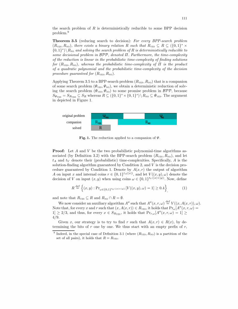
Applying Theorem 3.5 to a BPP-search problem (Ryes, Rno) that is a companionof some search problem (Ψyes, Ψno), we obtain a deterministic reduction of solv-ing the search problem (Ψyes, Ψno) to some promise problem in BPP, becauseSΨyes

= SRyes⊆ SR whereas R ⊆ (0, 1∗×0, 1∗)\Rno ⊆ Ψyes. The argument

in depicted in Figure 1.

Ψ ΨRR

YES

YES NO

NO

R

original problem

solved

companion

Fig. 1. The reduction applied to a companion of Ψ .

Proof: Let A and V be the two probabilistic polynomial-time algorithms as-sociated (by Definition 3.2) with the BPP-search problem (Ryes, Rno), and lettA and tV denote their (probabilistic) time-complexities. Specifically, A is thesolution-finding algorithm guaranteed by Condition 2, and V is the decision pro-cedure guaranteed by Condition 1. Denote by A(x, r) the output of algorithmA on input x and internal coins r ∈ 0, 1tA(|x|), and let V ((x, y), ω) denote thedecision of V on input (x, y) when using coins ω ∈ 0, 1tV (|x|+|y|). Now, define

Rdef=

(x, y) : Prω∈0,1tV (|x|+|y|) [V ((x, y), ω) = 1] ≥ 0.4

,(1)

and note that Ryes ⊆ R and Rno ∩R = ∅.We now consider an auxiliary algorithm A′′ such that A′′(x, r, ω)

def= V ((x, A(x, r)), ω).

Note that, for every x and r such that (x, A(x, r)) ∈ Ryes, it holds that Prω[A′′(x, r, ω) =1] ≥ 2/3, and thus, for every x ∈ SRyes

, it holds that Prr,ω[A′′(x, r, ω) = 1] ≥4/9.

Given x, our strategy is to try to find r such that A(x, r) ∈ R(x), by de-termining the bits of r one by one. We thus start with an empty prefix of r,

9 Indeed, in the special case of Definition 3.1 (where (Ryes, Rno) is a partition of theset of all pairs), it holds that R = Ryes.

112

denoted r′, and in each iteration we try to extend r′ by one bit. Assuming thatx ∈ SRyes

(which can be verified by a single BPP-query),10 we try to maintainthe invariant

Prr′′∈0,1m−|r′|,ω∈0,1ℓ [A′′(x, r′r′′, ω) = 1] ≥ 4

9− |r

′|25m ,

(2)

where m = tA(|x|) and ℓ = tV (|x| + m). Note that this invariant holds initially

(for the empty r′), and that if it holds for r′ ∈ 0, 1m, then necessarily ydef=

A(x, r) ∈ R(x) (since in this case Eq. (2) implies that Prω[V ((x, y), ω) = 1] ≥49 − 0.04 > 0.4).

In view of the foregoing, we focus on the design of a single iteration. Ourstrategy is to rely on an oracle for the promise problem ΠA′′ that consists of

yes-instances (x, 1m, r′) such that Prr′′,ω[A′′(x, r′r′′, ω) = 1] ≥ 49 −

|r′|−125m and

no-instances (x, 1m, r′) such that Prr′′,ω[A′′(x, r′r′′, ω) = 1] < 49 −

|r′|25m , where

in both cases the probability is taken uniformly over r′′ ∈ 0, 1m−|r′| (andω ∈ 0, 1ℓ). The oracle ΠA′′ is clearly in BPP (e.g., consider a probabilisticpolynomial-time algorithm that on input (x, 1m, r′) estimates Prr′′,ω[A′′(x, r′r′′, ω) =1] up to an additive term of 1/50m with error probability at most 1/3, by takinga sample of O(m2) random pairs (r′′, ω)).

In each iteration, which starts with some prefix r′ that satisfies Eq. (2), wemake a single query to the oracle ΠA′′ ; specifically, we query ΠA′′ on (x, 1m, r′0).If the oracle answers positively, then we extend the current prefix r′ with 0 (i.e.,we set r′ ← r′0), and otherwise we set r′ ← r′1.

The point is that if Prr′′∈0,1m−|r′|,ω[A′′(x, r′r′′, ω) = 1] ≥ 49 −

|r′|25m , then

there exists σ ∈ 0, 1 such that Prr′′′∈0,1m−|r′|−1,ω[A′′(x, r′σr′′′, ω) = 1] ≥49 −

|r′|25m = 4

9 −|r′σ|−1

25m , which means that (x, 1m, r′σ) is a yes-instance. Thus,if Π answers negatively to the query (x, 1m, r′0), then (x, 1m, r′0) cannot be ayes-instance, which implies that (x, 1m, r′1) is a yes-instance, and the invarianceof Eq. (2) holds for the extended prefix r′1. On the other hand, if Π = ΠA′′

answers positively to the query (x, 1m, r′0), then (x, 1m, r′0) cannot be a no-instance, and the invariance of Eq. (2) holds for the extended prefix r′0. Weconclude that each iteration of our reduction preserves the said invariance.

To verify the furthermore-part, we note that the reduction consists of tA(|x|)iterations, where in each iteration a query is made to Π and some very simplesteps are taken. In particular, each query made is simply related to the previousone (i.e., can be obtained from it in constant time), and so the entire reductionhas time complexity O(tA). The time complexity of Π on inputs of the formy = (x, 1m, r′) is O(m2) ·O(tV (|x|+m)) = O(|y|2 · tV (|y|)). The theorem follows.

10 Note that we do not care what happens when x violates the promise, whereas dis-tinguishing SRyes

from SRnocan be done in BPP (since Prr,ω[A′′(x, r, ω) = 1] is at

least 4/9 in the former case and at most 1/3 in the latter).

113

Digest. The proof of Theorem 3.5 follows the strategy of reducing NP-searchproblems to NP , except that more care is required in the process. This is re-flected in the invariance stated in Eq. (2) as well as in the fact that we make anessential use of promise problems (in the oracle).

Approximations. In light of the foregoing discussion (i.e., Observation 3.4), everyapproximation problem that has a probabilistic FPTAS can be deterministicallyreduced to BPP. Thus:

Corollary 3.6 (implication for FPTAS): If BPP = P, then every function thathas a probabilistic fully polynomial-time approximation scheme (FPTAS) alsohas such a deterministic scheme. Furthermore, for every polynomial p, thereexists a polynomial p′ such that if the probabilistic scheme runs in time p, thenthe deterministic one runs in time p′.

The furthermore part is proved by using the furthermore parts of Observation 3.3and Theorem 3.5 as well as a completeness feature of BPtime(·). Specifically,by combining the aforementioned reductions, we infer that the approximationproblem (which refers to instances of the form 〈x, 1m〉) is (deterministically) p1-time reducible to a problem in BPtime(p2), where p1(n) = O(p(n)) and p2(n) =O(n2 · p(n)). Next, we use the fact that BPtime(p2) has a complete problem,where completeness holds under quadratic-time reductions (which prepend theinput by the original problem’s description and pad it with a quadratic numberof zeros).11 The point is that this complete problem only depends on p2, whichin turn is uniquely determined by p. The hypothesis (i.e., BPP = P) impliesthat this BPtime(p2)-complete problem is in Dtime(p3) for some polynomialp3, which is solely determined by p2, and the claim follows for p′ = p3p2

1. Indeed,we have also established en passant the following result, which is of independentinterest.

Proposition 3.7 If BPP = P, then, for every polynomial p, there exists apolynomial p′ such that BPtime(p) ⊆ Dtime(p′).

Indeed, by the Dtime Hierarchy Theorem, it follows that, if BPP = P , then, forevery polynomial p, there exists a polynomial p′′ such that Dtime(p′′) containsproblems that are not in BPtime(p).

Constructions of varying quality. While the foregoing discussion of approxi-mation schemes is related to our previous proofs of the main result (see theAppendix), the following discussion is more related to the current proof (as pre-sented in Section 4.2). We consider general construction problems, which are de-fined in terms of a quality function q :0, 1∗→ [0, 1], when for a given n we needto construct an object y ∈ 0, 1n such that q(y) = 1. Specifically, we consider

11 The quadratic padding of x allows p2(|x|) steps of M(x) to be emulated in timeeO(|M | · p2(|x|)), which is upper-bounded by p2((|M | + |x|)2), assuming that p2 is(say) at least quadratic.

114

such construction problems that can be solved in probabilistic polynomial-timeand have a FPTAS for evaluating the quality of candidate constructions. Oneinteresting special case corresponds to rigid construction problems in which thefunction q is Boolean (i.e., candidate constructions have either value 0 or 1). Inthis special case (e.g., generating an n-bit long prime) the requirement that qhas a FPTAS is replaced by requiring that the set q−1(1) is in BPP.

Proposition 3.8 (derandomizing some constructions): Consider a generalized

construction defined via a quality function q that has a FPTAS, and let Rqdef=

((1n, 1m), y) : y∈0, 1n ∧ q(y)>1− (1/m). Suppose that there exists a prob-abilistic polynomial-time algorithm that solves the search problem of Rq. Then,if BPP = P, then there exists a deterministic polynomial-time algorithm thatsolves the search problem of Rq.

For example, if BPP = P , then n-bit long primes can be found in determin-istic poly(n)-time. On the other hand, the treatment can be generalized toconstructions that need to satisfy some auxiliary specification, captured by anauxiliary input x (e.g., on input a prime x = P find a quadratic non-residue

mod P ). In this formulation, Rqdef= ((x, 1m), y) : q(x, y) > 1 − (1/m), where

q : 0, 1∗×0, 1∗ → [0, 1] can also impose length restrictions on the desiredconstruct.

Proof: Consider the BPP-search problem (Πyes, Πno), where Πyes = ((1n, 1m), y) :y ∈0, 1n ∧ q(y)> 1 − (1/2m) and Πno = ((1n, 1m), y) : y ∈ 0, 1n ∧ q(y)≤1− (1/m). Note that (Πyes, Πno) is a companion of the search problem Rq, andapply Theorem 3.5.

Corollary 3.9 (a few examples): If BPP = P, then there exist deterministicpolynomial-time algorithms for solving the following construction problems.

1. For any fixed c > 7/12, on input N , find a prime in the interval [N, N +N c].2. On input a prime P and 1d, find an irreducible polynomial of degree d over

GF(P ).Recall that finding a quadratic non-residue modulo P is a special case.12.

3. For any fixed ǫ > 0 and integer d > 2, on input 1n, find a d-regular n-vertexgraph with second eigenvalue having absolute value at most 2

√d− 1 + ǫ.

The foregoing items are based on the density of the corresponding objects in anatural (easily sampleable) set. Specifically, for Item 1 we rely on the densityof prime numbers in this interval [13], for Item 2 we rely on the density ofirreducible polynomials [6], and for Item 3 we rely on the density of “almostRamanujan” graphs [5].13 In all cases there exist deterministic polynomial-timealgorithms for recognizing the desired objects.

12 Since if X2 + bX + c is irreducible, then so is (X + (b/2))2 + (c − (b/2)2), and itfollows that (c − (b/2)2) is a non-residue

13 Recall that Ramanujan graphs are known to be constructable only for specific valuesof d and of n.

115

4 Canonical Derandomizers

In Section 4.1 we present and motivate the rather standard notion of a canoni-cal derandomizer, which is the notion to which most of this work refers to. Ourmain result, the reversing of the pseudorandomness-to-derandomization trans-formation is presented in Section 4.2. One tightening, which allows to derive anequivalence, is presented in Section 4.3, which again refers to a rather standardnotion (i.e., of “effectively placing BPP in P”). An alternative equivalence isderived in Section 4.4, which refers to a (seemingly new) notion of a targetedcanonical derandomizer.

4.1 The definition

We start by reviewing the most standard definition of canonical derandomizers(cf., e.g., [8, Sec. 8.3.1]). Recall that in order to “derandomize” a probabilisticpolynomial-time algorithm A, we first obtain a functionally equivalent algorithmAG that uses a pseudorandom generator G in order to reduce the randomness-complexity of A, and then take the majority vote on all possible executions ofAG (on the given input). That is, we scan all possible outcomes of the coin tossesof AG(x), which means that the deterministic algorithm will run in time thatis exponential in the randomness complexity of AG. Thus, it suffices to have apseudorandom generator that can be evaluated in time that is exponential in itsseed length (and polynomial in its output length).

In the standard setting, algorithm AG has to maintain A’s input-output be-havior on all (but finitely many) inputs, and so the pseudorandomness propertyof G should hold with respect to distinguishers that receive non-uniform ad-vice (which models a potentially exceptional input on which A(x) and AG(x)are sufficiently different). Without loss of generality, we may assume that A’srunning-time is linearly related to its randomness complexity, and so the relevantdistinguishers may be confined to linear time. Similarly, for simplicity (and bypossibly padding the input x), we may assume that both complexities are lin-ear in the input length, |x|. (Actually, for simplicity we shall assume that bothcomplexities just equal |x|, although some constant slackness seems essential.)Finally, since we are going to scan all possible random-pads of AG and rule bymajority (and since A’s error probability is at most 1/3), it suffices to requirethat for every x it holds that |Pr[A(x) = 1]− Pr[AG(x) = 1]| < 1/6. This leadsto the pseudorandomness requirement stated in the following definition.

Definition 4.1 (canonical derandomizers, standard version [8, Def, 8.14])14:Let ℓ :N→N be a function such that ℓ(n) > n for all n. A canonical derandom-izer of stretch ℓ is a deterministic algorithm G that satisfies the following twoconditions.

14 To streamline our exposition, we preferred to avoid the standard additional step ofreplacing D(x, ·) by an arbitrary (non-uniform) Boolean circuit of quadratic size.

116

(generation time): On input a k-bit long seed, G makes at most poly(2k · ℓ(k))steps and outputs a string of length ℓ(k).

(pseudorandomness): For every (deterministic) linear-time algorithm D, all suf-ficiently large k and all x ∈ 0, 1ℓ(k), it holds that

|Pr[D(x, G(Uk)) = 1] − Pr[D(x, Uℓ(k)) = 1] | <1

6. (3)

The algorithm D represents a potential distinguisher, which is given two ℓ(k)-bitlong strings as input, where the first string (i.e., x) represents a (non-uniform)auxiliary input and the second string is sampled either from G(Uk) or from Uℓ(k).When seeking to derandomize a linear-time algorithm A, the first string (i.e., x)represents a potential main input for A, whereas the second string represents apossible sequence of coin tosses of A (when invoked on a generic (primary) inputx of length ℓ(k)).

Towards a uniform-complexity variant. Seeking a uniform-complexity analogueof Definition 4.1, the first thing that comes to mind is the following definition.

Definition 4.2 (canonical derandomizers, a uniform version): As Definition 4.1,except that the original pseudorandomness condition is replaced by

(pseudorandomness, revised): For every (deterministic) linear-time algorithm D,it is infeasible, given 1ℓ(k), to find a string x ∈ 0, 1ℓ(k) such that Eq. (3)does not hold. That is, for every probabilistic polynomial-time algorithm Fsuch that |F (1ℓ(k))| = ℓ(k), there exists a negligible function negl such thatif x← F (1ℓ(k)), then Eq. (3) holds with probability at least 1− negl(ℓ(k)).

When seeking to derandomize a probabilistic (linear-time) algorithm A, the aux-iliary algorithm F represents an attempt to find a string x ∈ 0, 1ℓ(k) on whichA(x) behaves differently depending on whether it is fed with random bits (i.e.,Uℓ(k)) or with pseudorandom ones produced by G(Uk).

Note that if there exists a canonical derandomizer of exponential stretch (i.e.,ℓ(k) = exp(Ω(k))), then BPP is “effectively” in P in the sense that for everyproblem in BPP there exists a deterministic polynomial-time algorithm A suchthat it is infeasible to find inputs on which A errs. We hoped to prove thatBPP = P implies the existence of such derandomizers, but do not quite provethis. Instead, we prove a closely related assertion that refers to the followingrevised notion of a canonical derandomizer, which is implicit in [16]. In thisdefinition, the finder F is incorporated in the distinguisher D, which in turn isan arbitrary probabilistic algorithm that is allowed some fixed polynomial-time(rather than being deterministic and linear-time).15 (In light of the central role ofthis definition in the current work, we spell it out rather than use a modificationon Definition 4.1 (as done in Definition 4.2).)

15 Thus, Definition 4.2 and Definition 4.3 are incomparable (when the time boundt is a fixed polynomial). On the one hand, Definition 4.3 seems weaker becausewe effectively fix the polynomial time bound of F (which is incorporated in D).On the other hand, Definition 4.3 seems stronger because D itself is allowed to

117

Definition 4.3 (canonical derandomizers, a revised uniform version): Let ℓ, t ::N→N be functions such that ℓ(n) > n for all n. A t-robust canonical derandom-izer of stretch ℓ is a deterministic algorithm G that satisfies the following twoconditions.

(generation time (as in Definition 4.1)): On input a k-bit long seed, G makes atmost poly(2k · ℓ(k)) steps and outputs a string of length ℓ(k).

(pseudorandomness, revised again): For every probabilistic t-time algorithm Dand all sufficiently large k, it holds that

|Pr[D(G(Uk)) = 1] − Pr[D(Uℓ(k)) = 1] | <1

t(ℓ(k)). (4)

Note that, on input an ℓ(k)-bit string, the algorithm D runs for at mostt(ℓ(k)) steps.

The pseudorandomness condition implies that, for every linear-time D′ and everyprobabilistic t-time algorithm F (such that |F (1n)| = n for every n), it holdsthat

|Pr[D′(F (1ℓ(k)), G(Uk)) = 1] − Pr[D′(F (1ℓ(k)), Uℓ(k)) = 1] | <1

t(ℓ(k)). (5)

Note that if, for every x, there exists a σ such that Pr[D′(x, U|x|) = σ] ≥ 1 −(1/3t(|x|)) (as is the case when D′ arises from an “amplified” BPP decisionprocedure), then the probability that F (1ℓ(k)) finds an instance x ∈ 0, 1ℓ(k)

on which D′(x, G(Uk)) leans in the opposite direction (i.e., Pr[D′(x, U|x|) 6=σ] ≥ 1/2) is smaller than 3/t(ℓ(k)). A more general (albeit quantatively weaker)statement is proved next.

Proposition 4.4 (on the effect of canonical derandomizers): For t :N→N suchthat t(n) > (n log n)3, let G be a t-robust canonical derandomizer of stretch ℓ.Let A be a probabilistic linear-time algorithm, and let AG be as in the foregoingdiscussions (i.e., AG(x, s) = A(x, G(s))). Then, for every probabilistic (t/2)-timealgorithm F and all sufficiently large k, the probability that F (1ℓ(k)) hits the set∇A,G(k) \BA(k) is at most 40/t(ℓ(k))1/3, where

∇A,G(k)def=

x ∈ 0, 1ℓ(k) : |Pr[AG(x, Uk) = 1] − Pr[A(x, Uℓ(k)) = 1] | >

1

3

(6)

BA(k)def=

x ∈ 0, 1ℓ(k) :

1

t(ℓ(k))1/3< Pr[A(x, Uℓ(k)) = 1] < 1− 1

t(ℓ(k))1/3

.

(7)

be probabilistic and run in time t (whereas in Definition 4.2 these privileges areonly allowed to F , which may be viewed as a preprocessing step). Indeed, if Erequires exponential size circuits, then there exist pseudorandom generators thatsatisfy one definition but not the other: On the one hand, this assumption yieldsthe existence of a non-uniformly strong canonical pseudorandom generator (i.e.,satisfying Definition 4.1) of exponential stretch [15] that is not p-robust (i.e., failsDefinition 4.3), for some sufficiently large polynomial p. On the other hand, theassumption implies BPP = P , which leads to the opposite separation described atthe end of Section 4.2.

118

That is, BA(·) denotes the set of inputs x on which A(x) = A(x, U|x|) is not“almost determined” and ∇A,G(·) denotes the set of inputs x on which there isa significant discrepancy between the distributions A(x) and AG(x).

The forgoing discussion refers to the special case in which BA(k) = ∅. In general,if A is a decision procedure of negligible error probability (for some promiseproblem),16 then AG is essentially as good as A, since it is hard to find aninstance x that matters (i.e., one on which A’s error probability is negligible) onwhich AG errs (with probability greater than, say, 0.4). This leads to “effectivelygood” derandomization of BPP. In particular, if G has exponential stretch, thenBPP is “effectively” in P .

Proof: Suppose towards the contradiction that there exist algorithms A and Fthat violate the claim. For each σ ∈ 0, 1, we consider the following probabilistict-time distinguisher, denoted Dσ. On input r (which is drawn from either Uℓ(k)

or G(Uk)), the distinguisher Dσ behaves as follows.

1. Obtains x← F (1|r|).

2. Approximates p(x)def= Pr[A(x, U|x|) = σ], obtaining an estimate, denoted

p(x), such that Pr[|p(x)− p(x)| ≤ t(|x|)−1/3] = 1− negl(|x|).3. If p(x) < 1− 2t(|x|)−1/3, then Dσ halts with output 0.

4. Otherwise (i.e., p(x) ≥ 1−2t(|x|)−1/3), Dσ invokes A on (x, r), and outputs 1if and only if A(x, r) = σ. (Indeed, the actual input r is only used in thisstep.)

We stress that Dσ only approximate the value of p(x) = Pr[A(x, U|x|)=σ] (i.e., itdoes not approximate the value of Pr[A(x, G(Uℓ−1(|x|))) = σ], which would haverequired invoking G). Observe that Dσ runs for at most t(|r|) steps, because the

approximation of p(x) amounts to O(t(|r|)2/3) invocations of A(x), whereas eachinvocation costs O(|r|) time (including the generation of truly random coins forA).

Let qσ(k) denote the probability that, on an ℓ(k)-bit long input, algorithmDσ moves to the final (input dependent) step, and note that qσ(k) is independentof the specific input r ∈ 0, 1ℓ(k). Assuming that |p(x)− p(x)| ≤ t(|x|)−1/3 (forthe string x selected at the first step), if the algorithm moves to the final step,then p(x) > 1−3t(|x|)−1/3. Similarly, if p(x) > 1−t(|x|)−1/3, then the algorithmmoves to the final step. Thus, the probability that Dσ(Uℓ(k))) outputs 1 is at

least (1 − negl(ℓ(k))) · qσ(k) · (1 − 3t(|x|)−1/3), which is greater than qσ(k) −4t(|x|)−1/3. On the other hand, by the contradiction hypothesis, there exists a σsuch that with probability at least 20t(ℓ(k))−1/3, it holds that F (1ℓ(k)) hits theset ∇A,G(k) ∩ Sσ,A(k), where

Sσ,A(k)def=

x ∈ 0, 1ℓ(k) : Pr[A(x, Uℓ(k)) = σ] ≥ 1− 1

t(ℓ(k))1/3

.

(8)

16 That is, BA(·) contains only instances that violate the promise.

119

In this case (i.e., when x ∈ ∇A,G(k)∩Sσ,A(k)) it holds that p(x) > 1− t(|x|)−1/3

(since x ∈ Sσ,A(k)) and Pr[A(x, G(Uℓ−1(|x|)))=σ] < 2/3 (since x ∈ ∇A,G(k) and

p(x) > 1− t(|x|)−1/3). It follows that the probability that Dσ(G(Uk)) outputs 1is at most (qσ(k) − 20t(|x|)−1/3) · 1 + 20t(|x|)−1/3) · (2/3) + negl(ℓ(k)), whichis smaller than qσ(k) − 5t(|x|)−1/3. Thus, we derive a contradiction to the t-robustness of G, and the claim follows.

4.2 The main result

Our main result is that BPP = P implies the existence of canonical deran-domizers of exponential stretch (in the sense of Definition 4.3). We concludethat seeking canonical derandomizers of exponential stretch is “complete” withrespect to placing BPP in P (at least in the “effective” sense captured by Propo-sition 4.4).

Theorem 4.5 (on the completeness of canonical derandomization): If BPP =P, then, for every polynomial p, there exists a p-robust canonical derandomizerof exponential stretch.

The proof of Theorem 4.5 is inspired by the study of pseudorandomness withrespect to deterministic (uniform p-time) observers, which was carried out byGoldreich and Wigderson [9]. Specifically, for every polynomial p, they presenteda polynomial-time construction of a sample space that fools any p-time determin-istic next-bit test. They observed that an analogous construction with respect togeneral (deterministic p-time) tests (i.e., distinguishers) would yield some non-trivial derandomization results (e.g., any unary set in BPP would be placed inP). Thus, they concluded that there is a fundamental gap between probabilisticand deterministic polynomial-time observers. Our key observation is that thisgap may disappear if BPP = P . Specifically, the hypothesis BPP = P allowsus to derandomize a trivial “probabilistic polynomial-time construction” of acanonical derandomizer.

Proof: Our starting point is the fact that, for some exponential function ℓ, withvery high probability, a random function G : 0, 1k → 0, 1ℓ(k) satisfies thepseudorandomness requirement associated with 2p-robust canonical derandom-izers. Furthermore, given the explicit description of any function G : 0, 1k →0, 1ℓ(k), we can efficiently distinguish between the case that G is 2p-robust andthe case that G is not p-robust.17 Thus, the construction of a suitable pseudoran-dom generator is essentially a BPP-search problem. Next, applying Theorem 3.5,we can deterministically reduce this construction problem to BPP. Finally, us-ing the hypothesis BPP = P , we obtain a deterministic construction. Detailsfollow.17 Formally, the asymptotic terminology of p-robustness is not adequate for discussing

finite functions mapping k-bit long strings to ℓ(k)-bit strings. However, as detailedbelow, what we mean is distinguishing (in probabilistic polynomial-time) betweenthe case that G is “2p-robust” with respect to a given list of p-time machines andthe case that G is not “p-robust” with respect to this list.

120

Let us fix an arbitrary polynomial p, and consider a suitable exponentialfunction ℓ (to be determined later). Our aim is to construct a sequence of map-pings G : 0, 1k→0, 1ℓ(k), for arbitrary k ∈ N, that meets the requirementsof a p-robust canonical derandomizer. It will be more convenient to construct asequence of sets S = ∪k∈NSℓ(k) such that Sn ⊆ 0, 1n, and let G(i) be the ith

string in Sℓ(k), where i ∈ [2k] ≡ 0, 1k. (Thus, the stretch function ℓ : N→N

satisfies ℓ(log2 |Sn|) = n, whereas we shall have |Sn| = poly(n), which impliesℓ(O(log n)) = n and ℓ(k) = exp(Ω(k)).) The set Sn should be constructed inpoly(n)-time (so that G is computable in poly(2k·ℓ(k))-time), and the pseudoran-domness requirement of G coincides with requiring that, for every probabilisticp-time algorithm D, and all sufficiently large n, it holds that18

∣∣∣∣∣Pr[D(Un)=1]− 1

|Sn|·

∑

s∈Sn

Pr[D(s)=1]

∣∣∣∣∣ <1

p(n) .

(9)

Specifically, we consider an enumeration of (modified)19 probabilistic p-time ma-chines, and focus on fooling (for each n) the p(n) first machines, where foolinga machine D means that Eq. (9) is satisfied (w.r.t this D). Note that, with

overwhelmingly high probability, a random set Sn of size K = O(p(n)2) satisfiesEq. (9) (w.r.t the p(n) first machines). Thus, the following search problem, de-

noted CON(p), is solvable in probabilistic O(p(n)2 · n)-time: On input 1n, find aK-subset Sn of 0, 1n such that Eq. (9) holds for each of the p(n) first machines.

Next, consider the following promise problem CC(p) (which is a companionof CON(p)). The valid instance-solution pairs of CC(p) are pairs (1n, Sn) such thatfor each of the first p(n) machines Eq. (9) holds with p(n) replaced by 2p(n), andits invalid instance-solution pairs are pairs (1n, Sn) such that for at least one ofthe first p(n) machines Eq. (9) does not hold. Note that CC(p) is a BPP-searchproblem (as per Definition 3.2), and that it is indeed a companion of CON(p)

(as per Observation 3.3). Thus, by Theorem 3.5,20 solving the search problemCON(p) is deterministically (polynomial-time) reducible to some promise problemin BPP. Finally, using the hypothesis BPP = P , the theorem follows.

Observation 4.6 (on the exact complexity of the construction): Note that (byTheorem 3.5) the foregoing reduction of CON(p) to BPP runs in time t(n) =

18 In [9, Thm. 2] the set Sn was only required to fool deterministic tests of the next-bittype.

19 Recall that one cannot effectively enumerate all machines that run within somegiven time bound. Yet, one can enumerate all machines, and modify each machinein the enumeration such that the running-time of the modified machine respects thegiven time bound, while maintaining the functionality of the original machines inthe case that the original machine respects the time bound. This is done by simplyincorporating a time-out mechanism.

20 See also the discussion just following the statement of Theorem 3.5, which assertsthat if the search problem of a companion of Π is reducible to BPP then the sameholds for Π .

121

O(p(n)2 · n), whereas the reduction is to a problem in quartic-time, becausethe verification problem associated with CC(p) is in sub-quadratic probabilistictime.21 Thus, assuming that probabilistic quartic-time is in Dtime(p4), for somepolynomial p4 (see Proposition 3.7), it follows that CON(p) ∈ Dtime(p′), where

p′(n) = p4(t(n)) = O((p4 p2)(n)).

Observation 4.7 (including the seed in the output sequence): The constructionof the generator G (or the set Sn) can be modified such that for every s ∈ 0, 1kthe k-bit long prefix of G(s) equals s (i.e., the ith string in Sn starts with the(log2 |Sn|)-bit long binary expansion of i).

A separation between Definition 4.2 and Definition 4.3: The p-robust canonicalderandomizer constructed in the foregoing proof (or rather a small variant of it)does not satisfy the notion of a canonical derandomizer stated in Definition 4.2.Indeed, in this case, a (deterministic) polynomial-time finder F , which runs formore time than the foregoing generator, can find a string x that allows very fastdistinguishing. Details follow.

The variant that we refer to is different from the one used in the proofof Theorem 4.5 only in the details of the underlying randomized construction.Instead of selecting a random set of O(p(n)2) strings, we select m = O(p(n)3)strings in a pairwise independent manner. (This somewhat bigger set suffices tomake the probabilistic argument used in the proof of Theorem 4.5 go through.)Furthermore, we consider a specific way of generating such an m-long sequenceover 0, 1n: For b = log2 m and t = n/b, we generate an m-long sequence byselecting uniformly (r1, s1), ..., (rt, st) ∈ 0, 12b, and letting the ith string in them-long sequence be the concatenation of the t strings r1+i·s1,..., rt+i·st (wherethe arithmetics is of GF(2b)). (In the actual determintic construction of Sn (andG) a sutibale sequence ((r1, s1), ..., (rt, st)) ∈ 0, 12bt is found and fixed, andthe G(i) equals the concatenation of the t strings r1+i·s1,..., rt+i·st.) Referringto this specific construction, we propose the following attack:

– The finder F determines the set Sn (just as the generator does). In particular,F determines the elements r1, s1, r2, s2 used in its construction, finds α, β ∈GF(2b) such that αs1 + βs2 = 0 and (α, β) 6= (0, 0), lets γ = α · r1 + β · r2,and encodes (α, β, γ) in the 3b-bit long prefix of x.

– On input x (viewed as starting with the 3b-bit long prefix (α, β, γ) ∈ GF(2b)3)and a tested n-bit long string that is viewed as a sequence (z1, ..., zt) ∈GF(2b)t, the distinguisher D output 1 if and only if α · z1 + β · z2 = γ.

21 On input (1n, S) we need to compare the average performance of p(n) machineson S versus their average performance on 0, 1n, where each machine makes at

most p(n) steps. Recalling that |S| = K = eO(p(n)2), and that it suffices to get anapproximation of the performance on 0, 1n up to an additive term of 1/2p(n),

we conclude that the entire task can be performed in time p(n) · eO(p(n)2) · p(n) <(n + |S|n)2 (i.e., the number of machines times the number of experiments (which

is |S| + eO(p(n)2)) times the running time of one experiment).

122

Note that D(x, G(Uk)) is identically 1 (because α · (r1 + i · s1) + β · (r2 + i · s2)equals γ = α · r1 + β · r2 for every i ∈ [m]), whereas Pr[D(x, Uℓ(k)) = 1] = 2−b

(because a fixed non-zero linear combination of two random elements of GF(2b)is uniformly distributed in GF(2b)).

Non-resilience to multiple samples. The foregoing example also demonstratesthe non-resilience of Definition 4.3 to multiple samples. Specifically, consider a

distinguisher D that obtains three samples, denoted (z(1)1 , ..., z

(1)t ), (z

(2)1 , ..., z

(2)t ),

and (z(3)1 , ..., z

(3)t ) (each viewed as a t-long sequence over GF(2b)), and outputs 1

if and only if (z(1)1 − z

(2)1 ) · (z(2)

2 − z(3)2 ) = (z

(1)2 − z

(2)2 ) · (z(2)

1 − z(3)1 ). Then,

D(G(i1), G(i2), G(i3)) = 1 for every i1, i2, i3 ∈ [2k] (because G(i1)j − G(i2)j =(i1 − i2) · sj and G(i2)j −G(i3)j = (i2 − i3) · sj for every j ∈ [t], which impliesthat each of the two compared products equals (i1− i2)(i2 − i3) · s1s2), whereas

D(U(1)ℓ(k), U

(2)ℓ(k), U

(3)ℓ(k)) equals 1 with probability 2−b (because each of the two

compared products is uniformly distributed in GF(2b)).

4.3 A tedious tightening

Recall that we (kind of) showed that canonical derandomizers of exponentialstretch imply that BPP is “effectively” contained in P (in the sense detailed inDefinition 4.8), whereas BPP = P implies the existence of the former. In thissection we tighten this relationship by showing that the existence of canonicalderandomizers of exponential stretch also follows from the hypothesis that BPPis “effectively” (rather than perfectly) contained in P .

Definition 4.8 (effective containment): Let C1 and C2 be two classes of promiseproblems, and let t : N → N. We say that C1 is t-effectively contained in C2 iffor every Π ∈ C1 there exists Π ′ ∈ C2 such that for every probabilistic t-timealgorithm F and all sufficiently large n it holds that Pr[F (1n) ∈ ∇(Π, Π ′) ∩0, 1n] < 1/t(n), where ∇(Π, Π ′) denotes the symmetric difference between

Π = (Πyes, Πno) and Π ′ = (Π ′yes

, Π ′no

) (i.e., ∇(Π, Π ′)def= ∇(Πyes, Π

′yes

) ∪∇(Πno, Π ′

no), where ∇(S, S′)def= (S \ S′) ∪ (S′ \ S)).

Theorem 4.9 The following two conditions are equivalent.

1. For every polynomial p, it holds that BPP is p-effectively contained in P.2. For every polynomial p, there exists a p-robust canonical derandomizer of

exponential stretch.

Proof: We first prove that Condition 2 implies Condition 1. (Indeed, thisassertion was made several times in the foregoing discussions, and here we merelydetail its proof.)

Let Π = (Πyes, Πno) be an arbitrary problem in BPP, and consider the cor-responding probabilistic linear-time algorithm A (of negligible error probability)derived for a padded version of Π , denoted Ψ = (Ψyes, Ψno). Specifically, sup-pose that for some polynomial p0, it holds that Ψyes = x0p0(|x|)−|x| : x ∈ Πyes

123

and ditto for Ψno. Now, for any polynomial p, consider the promise problemΨ ′ = (Ψ ′

yes, Ψ′no) such that

Ψ ′yes

def= x ∈ Ψyes : Pr[AG(x) = 1] > 0.6 (10)

Ψ ′no

def= x ∈ Ψno : Pr[AG(x) = 1] < 0.4, (11)

where AG is the algorithm obtained by combining A with a p-robust derandom-izer G of exponential stretch ℓ (i.e., AG(x, s) = A(x, G(s)), where ℓ(|s|) = |x|).Then, Proposition 4.4 implies that for every probabilistic p-time algorithm Fand all sufficiently large k, it holds that

Pr[F (1ℓ(k)) ∈ ∇(Ψ, Ψ ′) ∩ 0, 1ℓ(k)] <40

p(ℓ(k))1/3,

(12)

because ∇(Ψ, Ψ ′)∩0, 1ℓ(k) is contained in ∇A,G(k)\BA(k), where ∇A,G(k) andBA(k) are as in Eq. (6) and Eq. (7), respectively. Now, since G has exponentialstretch, it follows that the randomness complexity of AG is logarithmic (in itsinput length). Thus, algorithm AG runs in polynomial-time, and we can alsofully derandomize it in polynomial-time (by invoking AG on all possible randompads). Concluding that Ψ ′ ∈ P , we further infer that the same holds with respectto the “unpadded version” of Ψ ′, denoted Π ′ = (Π ′

yes, Π′no); that is, we refer to

Π ′yes

= x : x0p0(|x|)−|x| ∈ Ψ ′yes and ditto for Π ′

no. Finally, since ∇(Π, Π ′) ∩

0, 1n equals x : x0p0(|x|)−|x| ∈ ∇(Ψ, Ψ ′)∩ 0, 1p0(n), it follows that for everyprobabilistic p p0-time algorithm F and all sufficiently large n, it holds that

Pr[F (1n) ∈ ∇(Π, Π ′) ∩ 0, 1n] < 40/p(p0(n))1/3. Noting that the same appliesto any Π ∈ BPP (and any polynomial p), we conclude that BPP is (p1/3/40)-effectively contained in P , for every polynomial p. This completes the proof thatCondition 2 implies Condition 1.

We now turn to proving the converse (i.e., that Condition 1 implies Condi-tion 2). The idea is to go through the proof of Theorem 4.5, while noting thata failure of the resulting generator (which is supposed to be p-robust) yieldscontradiction to the p′-effective containment of BPP in P , where p′ is a poly-nomial that arises from the said proof. Specifically, note that the hypothesisBPP = P is used in the proof of Theorem 4.5 to transform a probabilisticconstruction into a deterministic one. This transformation is actually a (deter-ministic) p3-time22 reduction (of the construction problem) to a fixed problemΠ in BPtime(pΠ) ⊆ BPP, where pΠ(m) = m4. We also note that all queriesmade by the reduction have length Θ(2k · ℓ(k)) (see the proof of Theorem 3.5,

and recall that 2k = O(p(ℓ(k))2)). Thus, the reduction fails only if at least one ofthe queries made by it is answered incorrectly by the problem in P that is usedto p′-effective place Π in P . Randomly guessing the the index of the (wronglyanswered) query (i ∈ [p(ℓ(k))3]), we may answer the prior (i − 1) queries byusing the fixed BPP algorithm for Π , and hit an n-bit long instance in the sym-metric difference with probability at least (1/p(n)) · (1/p(n)3), where n = ℓ(k)

22 See Observation 4.6, and use eO(p(n)2 · n) ≪ p(n)3, which holds for all practicalpurposes.

124

(and the probability bound is due to the distinguishing gap of at least 1/p,which arises from a wrongly answered query that is hit by our selection of i withprobability 1/p(n)3). For a sufficiently large polynomial p′, this contradicts thehypothesis that BPP is p′-effectively contained in P . Specifically, on input 1n,our probabilistic algorithm runs for time p(n)3 · pΠ(p(n)3) = p(n)15 and hits abad m-bit long string (on which the derandomization fails) with probability at

least 1/p(n)4, where m = Θ(O(p(n)2 · n)). Thus, setting p′(m) = m8 suffices.(Formally, the claim follows by considering a modified algorithm that on input

1m invokes the foregoing algorithm on input 1m1/8

.)

Comment. The second part of the foregoing proof actually establishes that thereexists a fixed polynomial p′ such that if BPP is p′-effectively contained in P, then,for every every polynomial p, there exists a p-robust canonical derandomizer ofexponential stretch. Thus, we obtain that BPP is p′-effectively contained in Pif and only if for every polynomial p BPP is p′-effectively contained in P . Wecomment that this result can be proved directly by a padding argument.

4.4 A different tightening (targeted generators)

The use of uniform-complexity notions of canonical derandomizers does not seemto allow deriving perfect derandomization (of the type BPP = P). As we saw,the problem is that exceptional inputs (in the symmetric difference between theoriginal problem and the one solved deterministically) need to be found in orderto yield a violation of the pseudorandomness condition. An alternative approachmay let the generator depend on the input for which we wish to derandomizethe execution of the original probabilistic polynomial-time algorithm. This sug-gests the following notion of a targeted canonical derandomizer, where both thegenerator and the distinguisher are presented with the same auxiliary input (or“target”).

Definition 4.10 (targeted canonical derandomizers): Let ℓ :N→N be a functionsuch that ℓ(n) > n for all n. A targeted canonical derandomizer of stretch ℓ is adeterministic algorithm G that satisfies the following two conditions.

(generation time): On input a k-bit long seed and an ℓ(k)-bit long auxiliary in-put, G makes at most poly(2k · ℓ(k)) steps and outputs a string of lengthℓ(k).

(pseudorandomness (targeted)): For every (deterministic) linear-time algorithmD, all sufficiently large k and all x ∈ 0, 1ℓ(k), it holds that

|Pr[D(x, G(Uk, x)) = 1] − Pr[D(x, Uℓ(k)) = 1] | <1

6. (13)

Definition 4.10 is a special case of related definitions that have appeared in [25,Sec. 2.4]. Specifically, Vadhan [25] studied auxiliary-input pseudorandom gener-ators (of the general-purpose type [1, 26]), while offering a general treatment in

125

which pseudorandomness needs to hold for an arbitrary set of targets (i.e., x ∈ Ifor some set I ⊆ 0, 1∗).23

The notion of a targeted canonical derandomizer is not as odd as it looks atfirst glance. Indeed, the generator is far from being general-purpose (i.e., it istailored to a specific x), but this merely takes to (almost) the limit the insight ofNisan and Wigderson regarding relaxations that are still useful towards deran-domization [19]. Indeed, even if we were to fix the distinguisher D, constructinga generator that just fools D(x, ·) is not straightforward, because we need to finda suitable “fooling set” deterministically (in polynomial-time).

Theorem 4.11 (another equivalence): Targeted canonical derandomizers of ex-ponential stretch exist if and only if BPP = P.

Proof: Using any targeted canonical derandomizer of exponential stretch weobtain BPP = P , where the argument merely follows the one used in the contextof non-uniformly strong canonical derandomizers (i.e., canonical derandomizersin the sense of Definition 4.1). Turning to the opposite direction, we observe thatthe construction undertaken in the proof of Theorem 4.5 can be carried out withrespect to the given auxiliary-input. In particular, the fixed auxiliary-input ismerely passed among the various algorithms, and the argument remains intact.The theorem follows.

Observation 4.12 (super-exponential stretch): In contrast to the situation withrespect to the prior notions of canonical derandomizers (of Definitions 4.1–4.3),24

targeted canonical derandomizer of super-exponential stretch may exist. Indeed,they exists if and only if targeted canonical derandomizer of exponential stretchexist. To see this note that the hypothesis BPP = P allows to carry out the proofof Theorem 4.5 for any stretch function. Specifically, for any super-exponentialfunction ℓ, when constructing the set Sn ⊂ 0, 1n it suffices to fool the first g(n)(linear-time) machines, where g is any unbounded and non-decreasing functionand fooling means keeping the distinguishability gap below 1/6. Using a functiong such that g(n) ≤ poly(n) allows to construct Sn in poly(n)-time, whereas using

g such that g(n) < 0.5 ·exp(2 ·(1/6)2 ·2ℓ−1(n)) guarantees that log2 |Sn| ≤ ℓ−1(n),and the claim follows.

23 His treatment vastly extends the original notion of auxiliary-input one-way functionsput forward in [20].

24 For Definitions 4.1 and 4.2 super-exponential stretch is impossible because we canencode in x ∈ 0, 1ℓ(k) the list of all (k +1)-bit long strings that do not appear as aprefix of any string in G(s) : s ∈ 0, 1k, which yields a linear-time distinguisherof gap at least 1/2. In case of Definition 4.3, super-exponential stretch is impossiblebecause of a distinguisher that output 1 if and only if the tested string starts with0k+1, and so has a distinguishing gap of at least 2−(k+1). Indeed, in both cases weruled out ℓ(k) ≥ 2k+1.

126

4.5 Relating the various generators

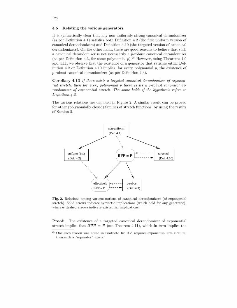
It is syntactically clear that any non-uniformly strong canonical derandomizer(as per Definition 4.1) satisfies both Definition 4.2 (the first uniform version ofcanonical derandomizers) and Definition 4.10 (the targeted version of canonicalderandomizers). On the other hand, there are good reasons to believe that sucha canonical derandomizer is not necessarily a p-robust canonical derandomizer(as per Definition 4.3, for some polynomial p).25 However, using Theorems 4.9and 4.11, we observe that the existence of a generator that satisfies either Def-inition 4.2 or Definition 4.10 implies, for every polynomial p, the existence ofp-robust canonical derandomizer (as per Definition 4.3).

Corollary 4.13 If there exists a targeted canonical derandomizer of exponen-tial stretch, then for every polynomial p there exists a p-robust canonical de-randomizer of exponential stretch. The same holds if the hypothesis refers toDefinition 4.2.

The various relations are depicted in Figure 2. A similar result can be provedfor other (polynomially closed) families of stretch functions, by using the resultsof Section 5.

non-uniform

(Def. 4.1)

uniform (1st)

(Def. 4.2)

(Def. 4.3)

p-robust

targetedBPP = P

BPP = P

effectively

(Def. 4.10)

Fig. 2. Relations among various notions of canonical derandomizers (of exponentialstretch). Solid arrows indicate syntactic implications (which hold for any generator),whereas dashed arrows indicate existential implications.

Proof: The existence of a targeted canonical derandomizer of exponentialstretch implies that BPP = P (see Theorem 4.11), which in turn implies the

25 One such reason was noted in Footnote 15: If E requires exponential size circuits,then such a “separator” exists.

127

existence of a p-robust canonical derandomizer of exponential stretch (see Theo-rem 4.5 or Theorem 4.9). Starting with a generator that satisfies Definition 4.2,one can easily prove that, for every polynomial p′, it holds that BPP is p′-effectively in P , where the proof is actually more direct than the correspondingdirection of Theorem 4.9. We are done by using the other direction of The-orem 4.9 (i.e., the construction of p-robust canonical derandomizer based onp′-effective containment of BPP in P).

5 Extension: the full “stretch vs time” trade-off

In this section we extend the ideas of the previous section to the study to gen-eral “stretch vs derandomization time” trade-off (akin to the general “hardnessvs randomness” trade-off). That is, here the standard hardness vs randomnesstrade-off takes the form of a trade-off between the stretch function of the canoni-cal derandomizer and time complexity of the deterministic class containing BPP.The robustness (resp., effectiveness) function will also be adapted accordingly.

Theorem 5.1 (Theorem 4.9, generalized): For every function t : N → N, thefollowing two conditions are equivalent.

1. For every two polynomials p0 and p, it holds that BPtime(p0) is (p t)-effectively contained in Dtime(poly(p t p0)).

2. For every polynomial p, there exists a (p t)-robust canonical derandomizer

of stretch ℓpt :N→N such that ℓpt(k)def= (pt)−1(2Ω(k)) = t−1(p−1(2Ω(k))).

Furthermore, the hidden constants in the Ω and poly notation are independentof the functions t, p and p0.

Indeed, Theorem 4.9 follows as a special case (when setting t(n) = n), whereasfor t(n) ≥ 2n both conditions hold trivially. Note that for t(n) = 2ǫn (resp.,t(n) = 2nǫ

), we get ℓpt(k) = Ω(k/ǫ)) (resp., ℓpt(k) = Ω(k)1/ǫ).

Proof: We closely follow the proof of Theorem 4.9, while detailing only thenecessary modifications. Starting with the proof that Condition 2 implies Con-dition 1, we let Π ∈ BPtime(p0), Ψ and A be as in the original proof. Now,for any polynomial p, we consider the promise problem Ψ ′ = (Ψ ′

yes, Ψ ′

no) such

that Ψ ′yes = x ∈ Ψyes : Pr[AG(x) = 1] > 0.6 and Ψ ′

no = x ∈ Ψno :Pr[AG(x) = 1] < 0.4, where AG is the algorithm obtained by combining Awith a (p t)-robust derandomizer G of stretch ℓpt. Then, Proposition 4.4 im-plies that for every probabilistic (p t)-time algorithm F and all sufficientlylarge k, it holds that Pr[F (1ℓ(k)) ∈ ∇(Ψ, Ψ ′) ∩ 0, 1ℓ(k)] < 40/(p t)1/3(ℓ(k)).Since G has stretch ℓpt, it follows that on input an n-bit string algorithm AG

uses ℓ−1pt(n) = O(log(p t)(n)) many coins, and thus we can also fully de-

randomize it in time poly((p t)(n)). Thus, Ψ ′ ∈ Dtime(poly(p t)), and itfollows that Π ′ ∈ Dtime(poly(p t p0)), where Π ′ denotes the “unpaddedversion” of Ψ ′. Concluding that Π is ((p t)1/3/40)-effectively contained in

128

Dtime(poly(p t p0)), and that the same holds for any Π ∈ BPtime(p0) andevery polynomial p, we have established that Condition 2 implies Condition 1.

We now turn to proving the converse (i.e., that Condition 1 implies Con-dition 2). Again, we merely go through the proof of Theorem 4.5, except thathere we construct a set Sn of size poly(p t)(n). Specifically, the discrepan-cies we aim at are linearly related to 1/(p t)(n), and we can afford spendingtime poly(p t)(n) in the construction. We shall indeed make use of this al-lowance, since we can only rely on the (t′-effective) containment of BPtime(p0)in Dtime(poly(p t p0)), where t′ = poly(p t) = poly(p) t. The rest of theargument proceeds analogously to the proof of Theorem 4.9. We note that theaforementioned hypothesis regarding BPtime(p0) is only used when determinis-tically reducing (in time poly(p t)) the construction of Sn to a fixed problem Πin BPtime(p0), where p0(m) = m4 (as in the proof of Theorem 4.9). Thus, thereduction fails only if at least one of the queries made by it is answered incor-

rectly by the problem in D def= Dtime(poly(p t p0)) that is used to t′-effective

place Π in D. Randomly guessing the the index of the (wrongly answered) query,we hit an m-bit long instance in the symmetric difference with probability atleast 1/poly(p(t(n))), where m = Ω(ℓ(k)), which contradicts the hypothesis thatBPtime(p0) is t′-effectively contained in D.26

6 Open Problems

We start by recalling the famous open problem regarding whether the a fullderandomization of standard decision problems implies the same for promiseproblems. That is, assuming that any decision problem in BPP is in P , does itfollow that BPP = P? 27

One problem that arises from the current work refers to the relationshipbetween the two uniform definitions of canonical derandomizers (i.e., Defini-tions 4.2 and 4.3). Recall (see Section 4.5) that the existence of generators (ofexponential stretch) that satisfy Definition 4.2 implies the existence of genera-tors (of exponential stretch) that satisfy Definition 4.3, but the converse is notclear.

Another open problem refers to the deriving of analogous results regardingthe derandomization ofAM (or AM∩coAM). Here the canonical derandomizershould be computable in non-deterministic poly(2k · ℓ(k))-time, where computa-tion by non-deterministic machines refers to the so called “single-value” model(see, e.g., [22] or [8, Def. 5.13]). The problem in reversing the “pseudorandomnessto derandomization” connection refers to a tension between the distinguishersused to argue about the derandomization versus our need to handle them in

26 Here, too, m = Θ( eO(p(t(n))2 · n) actually holds, and so it actually suffices to sett′(m) = poly(m).

27 Formally, let D denote the set of all promise problems having a trivial promise; thatis, a promise problem (Πyes, Πno) is in D if Πyes∪Πno = 0, 1∗. Then, the questionis whether BPP ∩ D = P ∩ D implies BPP = P .

129

the construction of the canonical derandomizer. We would welcome any result,even for a targeted version and even for derandomizing some subclass such asAM∩ coAM or SZK.

Finally, we return to the question raised in passing in Section 1.4. Specifically,we ask which search problems can be solved by deterministic polynomial-time re-ductions to BPP. Denoting the class of such search problems by C, we note thatTheorem 3.5 implies that C contains all search problems that have a companionthat is a BPP-search problem. The converse holds in the special case that thetarget of the reduction is a standard decision problem (and the reduced searchproblem has a trivial promise at the instance level (see below)). Let us con-sider the general case and see what happens. Suppose that the search problem(Ryes, Rno) that is reducible in deterministic polynomial-time to Π ∈ BPP. De-noting the oracle machine effecting the reduction by M , we consider the searchproblem (R′

yes, R′no) such that (x, y) ∈ R′

yes if Mf (x) = y for some f thatis consistent with Π and (x, y) ∈ R′

nootherwise.28 The correctness of the re-

duction implies that SR′yes⊇ SRyes

whereas R′no ⊇ Rno, which means that if

SRyes∪ SRno

= 0, 1∗, then (R′yes, R

′no) is a companion of (Ryes, Rno). Now

if Π is a standard decision problem, then f is unique; hence, R′yes

(x) is a sin-gleton if x ∈ SR′

yesand is empty otherwise (since SR′

no= 0, 1∗ \ SR′

yes). In

this case membership of (x, y) in R′yes

can be easily tested by checking whetherMΠ(x) = y. The same holds if the reduction is “smart” (i.e., avoids makingqueries that violate the promise, cf. [11]),29 but in general it is not clear whathappens.

Acknowledgments

We are grateful to Noga Alon, Or Meir, Madhu Sudan, and Avi Wigderson foruseful discussions on related issues. We also thank Or Meir, Dieter van Melke-beek, and Salil Vadhan for their comments on early drafts of this work.

References

1. M. Blum and S. Micali. How to Generate Cryptographically Strong Sequencesof Pseudo-Random Bits. SICOMP, Vol. 13, pages 850–864, 1984. Preliminaryversion in 23rd FOCS, pages 80–91, 1982.

2. B. Chor and O. Goldreich. On the Power of Two–Point Based Sampling.Jour. of Complexity, Vol 5, 1989, pages 96–106.

3. S. Even, A.L. Selman, and Y. Yacobi. The Complexity of Promise Problemswith Applications to Public-Key Cryptography. Inform. and Control, Vol. 61,pages 159–173, 1984.

28 Saying that f is consistent with Π = (Πyes, Πno) means that f(x) = 1 for everyx ∈ SΠyes

, whereas f(x) = 0 for every x ∈ SΠno. Indeed, the value of f on inputs

that violate the promise (i.e., x 6∈ SΠyes∪ SΠno

) is arbitrary.29 We note, however, that the reduction used in the proof of Theorem 3.5 is not smart.

Furthermore, we doudt that a smart reduction can be found.

130

4. L. Fortnow. Comparing Notions of Full Derandomization. In 16th CCC, pages28–34, 2001.

5. J. Friedman. A Proof of Alon’s Second Eigenvalue Conjecture. In 35th STOC,pages 720–724, 2003.

6. C.F. Gauss. Untersuchungen Uber Hohere Arithmetik. Chelsea publishingcompany, second edition, reprinted, New York, 1981.

7. O. Goldreich. Foundation of Cryptography: Basic Tools. Cambridge UniversityPress, 2001.

8. O. Goldreich. Computational Complexity: A Conceptual Perspective. Cam-bridge University Press, 2008.

9. O. Goldreich and A. Wigderson, On Pseudorandomness with respect to De-terministic Observers. In RANDOM’00, proceedings of the satellite workshops

of the 27th ICALP. Carleton Scientific (Proc. in Inform. 8), pages 77–84, 2000.See also ECCC, TR00-056.

10. S. Goldwasser and S. Micali. Probabilistic Encryption. JCSS, Vol. 28, No. 2,pages 270–299, 1984. Preliminary version in 14th STOC, 1982.

11. J. Grollmann and A.L. Selman. Complexity Measures for Public-Key Cryp-tosystems. SICOMP, Vol. 17 (2), pages 309–335, 1988.

12. D. Hochbaum (ed.). Approximation Algorithms for NP-Hard Problems. PWS,1996.

13. M.N. Huxley. On the Difference Between Consecutive Primes. Invent. Math.,Vol. 15, pages 164–170, 1972.

14. R. Impagliazzo, V. Kabanets, and A. Wigderson. In Search of an Easy Witness:Exponential Time vs Probabilistic Polynomial Time. JCSS, Vol. 65 (4), pages672–694, 2002. Preliminary version in 16th CCC, 2001.

15. R. Impagliazzo and A. Wigderson. P=BPP if E requires exponential circuits:Derandomizing the XOR Lemma. In 29th STOC, pages 220–229, 1997.

16. R. Impagliazzo and A. Wigderson. Randomness vs. Time: De-randomizationunder a uniform assumption. JCSS, Vol. 63 (4), pages 672–688, 2001. Prelim-inary version in 39th FOCS, 1998.

17. M. Jerrum, L. Valiant, and V.V. Vazirani. Random Generation of Combina-torial Structures from a Uniform Distribution. TCS, Vol. 43, pages 169–188,1986.

18. V. Kabanets and R. Impagliazzo. Derandomizing Polynomial Identity TestsMeans Proving Circuit Lower Bounds. Computational Complexity, Vol. 13,pages 1-46, 2004. Preliminary version in 35th STOC, 2003.

19. N. Nisan and A. Wigderson. Hardness vs Randomness. JCSS, Vol. 49, No. 2,pages 149–167, 1994. Preliminary version in 29th FOCS, 1988.

20. R. Ostrovsky and A. Wigderson. One-Way Functions are Essential for Non-Trivial Zero-Knowledge. In 2nd Israel Symp. on Theory of Computing and

Systems, IEEE Comp. Soc. Press, pages 3–17, 1993.21. O. Reingold, L. Trevisan, and S. Vadhan. Pseudorandom walks on regular

digraphs and the RL vs. L problem. In 38th STOC, pages 457–466, 2006. Seedetails in ECCC, TR05-022.

22. R. Shaltiel and C. Umans. Low-end Uniform Hardness vs Randomness Trade-offs for AM. SICOMP, Vol. 39, No. 3, pages 1006–1037, 2009. Preliminaryversion in 39th STOC, 2007.

23. L. Trevisan and S. Vadhan. Pseudorandomness and Average-Case ComplexityVia Uniform Reductions. Computational Complexity, Vol. 16 (4), pages 331–364, 2007. Preliminary version in 17th CCC, 2002.

131

24. C. Umans. Pseudo-random Generators for all Hardness. JCSS, Vol. 67 (2),pages 419–440, 2003. Preliminary version in 34th STOC, 2002.

25. S. Vadhan. An Unconditional Study of Computational Zero Knowledge.SICOMP, Vol. 36 (4), pages 1160–1214, 2006. Preliminary version in 45th

FOCS, 2004.26. A.C. Yao. Theory and Application of Trapdoor Functions. In 23rd FOCS,

pages 80–91, 1982.

132

Appendices: prior proofs of the main result (Theorem 4.5)

The current proof of Theorem 4.5 is the second simplification we found: It isa third incarnation of the same underlying principles, but it hides the originalinspiration to our ideas, which are rooted in [9]. Since we do have written recordsof these prior proofs, and since they may be of some interest, we decided toinclude them in the current appendix.

Our starting point was the work of Goldreich and Wigderson [9], whichstudied pseudorandomness with respect to (uniform) deterministic observers.In particular, they show how to construct, for every polynomial p, a generatorof exponential stretch that works in time polynomial in its output and fools alldeterministic p-time tests of the next-bit type (a la [1]). They observe that ananalogous construction with respect to general (deterministic p-time) tests (ordistinguishers) would yield some non-trivial derandomization results (e.g., anyunary set in BPP would be placed in P). Thus, they conclude that Yao’s result30

asserting that fooling all efficient next-bit tests implies fooling all efficient dis-tinguishers relies on the fact that the class of test includes probabilistic p-timealgorithms and not only deterministic ones.

Our key observation is that the gap between probabilistic next-bit tests anddeterministic ones essentially disappears if BPP = P . Actually, the gap disap-pears if we generalize the notion of next-bit tests so to allow the (deterministic)tester to output a guess of the probability that the next bit equals 1 (rather thana guess for the actual value of the next bit), and consider the correlation betweenthe corresponding random variables. Indeed, assuming that BPP = P , allows todeterministically emulate a probabilistic p-time next bit test by a (generalized)deterministic p′-time next bit test, where p′ is a polynomial that depends onlyon p. Plugging this into the construction of [9], which can be shown to fool also(generalized) deterministic p′-time next bit test, we obtain the desired generator(which produces ℓ-bit outputs in time poly(p′(ℓ))). A crucial point in the fore-going argument is that the next-bit test does not need to invoke the generator,which is not feasible because the generator runs for more time than the potentialtests.

The foregoing argument led to the first proof, which is presented in Ap-pendix A.2. Subsequently we found a more direct approach, which is presentedin Appendix A.1. This approach is more transparent and amenable to variationsthan the first one (but less so in comparison to the proof presented in Section 4.2).Specifically, rather than working with (generalized) next-bit tests, we directlywork with (probabilistic p-time) distinguishers, and adapt the argument of [9] toapply in this context. It turns out that in order for this to work, we only needto approximate the probability that a fixed probabilistic p-time distinguishersoutputs 1 when presented with random (ℓ− i)-bit long extensions of some fixedi-bit long strings, for i = 1, ..., ℓ. Assuming that BPP = P , allows to determin-istically approximate these probabilities (again, in p′-time, where p′ = poly(p)),

30 Attributed to oral presentations of [26].

133

and so we are done. Needless to say, the fact that such approximations sufficesis specific to (our adaptation of) the construction of [9].

A.1 An alternative proof of Theorem 4.5 (via derandomizing aFPTAS)

The alternative proof of Theorem 4.5 proceeds by generalizing the main idea thatunderlies the work of Goldreich and Wigderson [9], while using the hypothesis(i.e., BPP = P) to extend its scope to probabilistic (rather than deterministic)observers. Specifically, for every polynomial p, they presented a polynomial-time construction of a sample space that fools any p-time deterministic next-bittest. The construction is iterative, where in each iteration the next bit of eachstring in the sample space is determined such that the resulting space fools allrelevant next-bit tests. Here we consider any (p-time) probabilistic distinguisher,and seek to determine the next bit so that the probability that this distinguisheroutput 1 (on a random extension of the current sample space) is approximatelymaintained. Towards this end, we need to approximate the probability thata fixed p-time probabilistic algorithm outputs 1 on a random extension of thecurrent prefix. Our key observation is that, due to the hypothesis that BPP = P ,this quantity can be approximated in deterministic polynomial-time. The use ofthis hypothesis is far from being surprising, since (as noted before) the conclusionof Theorem 4.5 implies that, in some “effective” sense, BPP does equal P .

Proof: We follow the general outline of the proof of [9, Thm. 2], while comment-ing (mostly in footnotes) about the points of deviation. Let us fix an arbitrarypolynomial p, and consider a suitable exponential function ℓ (to be determinedlater). Our aim is to construct a sequence of mappings G : 0, 1k→0, 1ℓ(k),for arbitrary k ∈ N, that meets the requirements of a p-robust canonical de-randomizer. However, it will be more convenient to construct a sequence of setsS = ∪k∈NSℓ(k) such that Sn ⊆ 0, 1n, and let G(i) be the ith string in Sℓ(k),

where i ∈ [2k] ≡ 0, 1k. (Thus, the function ℓ :N→N satisfies ℓ(log2 |Sn|) = n,whereas we shall have |Sn| = poly(n).) The set Sn should be constructed inpoly(n)-time (so that G is computable in poly(2k · ℓ(k))-time), and the pseudo-randomness requirement of G coincides with requiring that, for every probabilis-tic p-time algorithm D, and all sufficiently large n, it holds that31

∣∣∣∣∣Pr[D(Un)=1]− 1

|Sn|·

∑

s∈Sn

Pr[D(s)=1]

∣∣∣∣∣ <1

p(n) .

(14)

Specifically, we consider an enumeration of (modified)32 probabilistic machinesrunning within time p(n) on input of length n, and focus on fooling the m =

31 In [9, Thm. 2] the set Sn was only required to fool deterministic tests of the next-bittype.

32 Recall that one cannot effectively enumerate all machines that run within somegiven time bound. Yet, one can enumerate all machines, and modify each machinein the enumeration such that the running-time of the modified machine respects the

134

m(n) < p(n) first machines in the sense of Eq. (14). Let ǫ = 1/p(n), and M bea generic machines that we wish to fool.

We construct Sn in (roughly) n iterations, such that in iteration i we con-struct Sn,i ⊆ 0, 1i. We start with Sn,k = 0, 1k, where k = 2 log2(2nm/ǫ),and let K = 2k. In the i+1st iteration, we consider the function fM : [K]→ [0, 1]representing the probability that M outputs 1 on a random extension of each ofthe K strings in Sn,i; that is, fM (j) = Pr[M(x(j)Un−i)=1], where x(j) is the jth

string in Sn,i ⊆ 0, 1i. (The function fM represents M ’s average output on allpossible (n− i)-bit long extensions of all strings in Sn,i.)

33 Our aim is to find avector u ∈ 0, 1K such that, for each machine M (among the first m machines),it holds that the average value of Pr[M(x(j)u[j]Un−i−1)=1] is ǫ/n-close to theaverage value of fM (j); that is,

∣∣∣∣∣∣1

K

∑

j∈[K]

Pr[M(x(j)u[j]Un−i−1)=1]− 1

K·

∑

j∈[K]

fM (j)

∣∣∣∣∣∣<

ǫ

n .(15)

Once such a vector u is found, we extend Sn,i into Sn,i+1 in the natural manner;that is,

Sn,i+1def= x(j)u[j] : where x(j) is the jth string in Sn,i ⊂ 0, 1i+1. (16)

It follows that Sndef= Sn,n satisfies Eq. (14), because, for each of the aforemen-

tioned M ’s and for each i ∈ [n− k, n− 1], it holds that

∣∣∣∣∣∣1

|Sn,i|·

∑

s∈Sn,i

Pr[M(s)=1]− 1

|Sn,i+1|·

∑

s∈Sn,i+1

Pr[M(s)=1]

∣∣∣∣∣∣<

ǫ

n(17)

since the terms in the l.h.s are represented by the function fM defined at the ith

iteration, whereas the terms in the r.h.s correspond to the function fM definedin the next iteration.

It remains to specify how a suitable vector u ∈ 0, 1K is found, in eachiteration. This is done by using a pairwise independent sample space for stringsof length K, while recalling that such spaces can be constructed in poly(K)-time(cf., e.g., [2]). Two issues arise:

1. Showing that such a sample space must always contain a suitable vec-tor u ∈ 0, 1K; that is, a vector u ∈ 0, 1K satisfies Eq. (15). This is

given time bound, while maintaining the functionality of the original machines inthe case that the original machine respects the time bound. This is done by simplyincorporating a time-out mechanism.

33 In contrast, in [9], the function fM (which is denoted vM there) represented M ’sattempt to guess the i + 1st bit of a string in Sn, based on the i-bit long prefix ofthat string. Furthermore, since in [9] the machine M is deterministic, the functionfM (there) can be constructed by invoking M on K different i-bit strings.

135

quite an immediate consequence of the fact that, when defining qM,j(σ)def=

Pr[M(x(j)σUn−i−1)=1], we can write Eq. (15) as

∣∣∣∣∣∣1

K

∑

j∈[K]

qM,j(u[j])− 1

K·

∑

j∈[K]

∑

σ∈0,1

qM,j(σ)

2

∣∣∣∣∣∣<

ǫ

n .(18)

Indeed, when u is selected from a pairwise-independent sample space of0, 1K, Eq. (18) holds with probability at least 1− (1/((ǫ/n)2K)), and theclaim follows whenever (ǫ/n)2K > m.Actually, we shall use the fact that, with probability at least 1−(1/((ǫ/2n)2K)),a modified version of Eq. (18) holds, where in the modification the upperbound ǫ/n is replaced by the (tighter) upper bound ǫ/2n.

2. Showing that we can distinguish in deterministic polynomial-time whether agiven vector u ∈ 0, 1K satisfies the aforementioned tighter form of Eq. (18)or violates Eq. (15).This issue hardly arose in [9], since there fM (j) referred to the output of adeterministic machine on fixed string (i.e., the jth string in Sn,i). But herefM (j) refers to the expected output of a probabilistic machine on a randomextension of a fixed string. Nevertheless, fM (j) can be approximated towithin an additive term of ǫ/4n by a simple probabilistic algorithm thatmerely invokes M sufficiently many (i.e., O(n/ǫ)2) times on such randomextensions, and ditto for qM,j(·). Now, using the hypothesis BPP = P andapplying Corollary 3.6,34 we conclude that qM,j(·) can be approximated well-enough (i.e., up to an additive term of ǫ/4n) by a deterministic polynomial-time algorithm. Formally, the approximation problem is defined for inputs ofthe form (M, 1n, x), where M and n are as above and x is a string of lengthat most n (i.e., in our application, x = x(j)σ ∈ 0, 1i+1, where x(j) is thejth string in Sn,i).

Thus, in each iteration we can find a vector u as desired, an consequently weconstruct the desired set Sn in time that is polynomial in n. The theorem follows.

Comment: The generator constructed in the foregoing proof does not satisfythe notion of a canonical derandomizer stated in Definition 4.2. Indeed, in thiscase, a (deterministic) polynomial-time finder F , which runs for more time thanthe foregoing generator, can find a string x that allows very fast distinguishing.Details follow.

Referring to the foregoing construction of a pseudorandom generator G, weshow how to find in polynomial-time a string x ∈ 0, 1ℓ(k) such that (x, G(Uk))and (x, Uℓ(k)) are easy to tell apart. Actually, we refer to a specific implemen-tation of the construction; that is, to a specific implementation of the pairwise

34 Formally, there is a problem here since we do not have a FPTAS for the quantitiesqM,j(·) ∈ [0, 1], but we do have a FPTAS for the quantities 1 + qM,j(·) ∈ [1, 2] andthis suffices here.

136

independence sample space, where the aspect we rely on is that this sample spaceis a vector space of low dimension.

Recall that the set Sn, which is the support of G(Uk) (for n = ℓ(k)), isconstructed by concatenating n vectors, where each vector is an 2k-bit longsequence taken from a pairwise independence sample space. Specifically, considerthe sample space generated by strings of length k+1 such that the jth coordinateof the vector generated by r1 · · · rk+1 ∈ 0, 1k+1 equals

∑k+1h=1 jhrh, where jh is

the hth bit in the (k +1)-bit long binary expansion of j ∈ [2k]. Thus, each of thevectors used in the construction of Sn reside in the very same (k+1)-dimensionalvector space.

Then, the finder F can just construct Sn (as done by G), and record thesequence uk+1, ..., un of vectors taken in each of the n− k iterations (or rathertheir succinct representation). In fact, it suffices to record the indices of a sub-sequence, of length d ≤ k +2, that sums-up to the all zero vector; that is, record(i1, ..., id) such that the sum of the vectors taken in iterations i1, ..., id equals

the all-zero vector (i.e.,∑d

h=1 uih= 0). Now, F just records such a sequence in

a prefix of x, and the distinguisher D just outputs the XOR value of the bitsthat appear in these positions. Clearly, D(x, z) = 0 for every z ∈ Sn, whereasPr[D(x, Uℓ) = 0] = 1/2.

A.2 Another alternative proof of Theorem 4.5 (via next-bit tests)

The alternative proof of Theorem 4.5 follows by combining two results: The firstis an unconditional result that asserts a generator that passes the next-bit testwith respect to deterministic observers, and the second is a conditional determin-istic analogue of the fact that next-bit unpredictability implies pseudorandom-ness. The first result is a technical generalization of [9, Thm. 2] (see Theorem A.2below), whereas the second result uses the hypothesis that BPP = P . The useof this hypothesis should not come at a surprise, since as noted before the con-clusion of Theorem 4.5 implies that in some “effective” sense BPP does equalP . (Thus, as observed in [9], an unconditional implication of the foregoing type,would yield an unconditional derandomization of BPP.)

Next-bit unpredictability, generalized. Let us first present a natural generalizationof the notion of next-bit unpredictability, which is pivotal to our argument.Recall that the standard notion refers to the probability of guessing the nextbit in a sequence, when given its prefix. That is, in the standard formulation,the predictor outputs a bit, and the question is whether this bit matches theactual next bit. Now, consider a generalization in which the predictor output itsestimate of the probability that the next bit is 1, and normalizing the “payoff”accordingly. That is, the generalized predictor outputs a probability p ∈ [0, 1],and gets payoff 2p− 1 if the outcome (of the next bit) is 1 and payoff 1− 2p ifthe outcome is 0. (In general, the payoff is (1− 2p) · (−1)σ, where σ denotes theoutcome of the next bit.) Note that such a generalization allows the capture theintuitive case that the predictor wishes to pass on the guess, collect no potentialgain but also suffer from no potential loss.

137

In the context of probabilistic algorithms, nothing is gained by this general-ization, because a a probabilistic predictor may maintain the expected payoff byreplacing the output p ∈ [0, 1] with a biased coin toss (i.e., a random Booleanvalue that is biased with probability p towards 1).35 But this generalizationseems more powerful in the context of deterministic predictors, and we shallthus refer to it.

It will be more convenient to replace prediction probabilities with correlation,as we have already done implicitly above. Thus, the predictors will output a valuein v ∈ [−1, +1] (rather than in [0, 1]) and collect the payoff v · (−1)σ, where σdenotes the outcome of the next bit. Thus, v corresponds to 1−2p in the forgoingdiscussion, and v · (−1)σ corresponds to the correlation of v with (−1)σ.

Definition A.1 (next bit unpredictability, generalized): For ℓ : N→ N, let G :0, 1∗ → 0, 1∗ be such that for every s ∈ 0, 1∗ it holds that |G(s)| = ℓ(|s|).– For ǫ : N → [0, 1], we say that A : N× 0, 1∗ → [−1, +1] has correlation at

most ǫ with the next bit of G if for all sufficiently large k and all i < ℓ(k), itholds that

E[A(1ℓ(k), x1, ..., xi) · (−1)xi+1] ≤ ǫ(ℓ(k)), (19)

where (x1, ..., xℓ(k))← G(s) for a uniformly selected s ∈ 0, 1k.We will often omit 1ℓ(k) from the list of inputs to A.

– We say that G is next-bit unpredictable by a class of algorithms A with respectto an advantage ǫ if every algorithm in A has correlation at most ǫ with thenext bit of G.We say that G is next-bit t-unpredictable if G is next-bit unpredictable withrespect to advantage 1/t by the class of deterministic t-time algorithms thathave output in [−1, +1].

By a straightforward extension of the ideas of [9], we obtain the following un-conditional result.

Theorem A.2 ([9, Thm. 2], generalized): For every polynomial p, there existan exponential function ℓ and a deterministic algorithm G that satisfies the firstcondition of Definition 4.3 such that G is next-bit p-unpredictable.

The original result was stated in terms of predicting probabilities, and corre-sponds to the special case in which the algorithm’s output is always in −1, +1(where, in this case, E[A(x1, ..., xi)·(−1)xi+1 ] equals 2·Pr[A(x1, ..., xi)=(−1)xi+1 ]−1). The original proof extends in a straightforward manner; see Appendix A.3.

The following result presents a conditional transformation from next-bit un-predictability (by deterministic algorithms) to pseudorandomness (which holdswith respect to probabilistic algorithms). This transformation relies on the factthat the hypothesis BPP = P allows for derandomizing potential probabilis-tic next-bit predictors, which are obtained (in the usual way) from potentialdistinguishers.

35 That is, the expected payoff with respect to a random variable ζ ∈ 0, 1 is main-tained, because the original payoff is E[(1 − 2p) · (−1)ζ ], whereas the payoff of theresulting Boolean predictor is p · E[(−1)ζ+1] + (1 − p) · E[(−1)ζ ].

138

Theorem A.3 (next-bit unpredictability implies pseudorandomness): If BPP =P, then, for every polynomial p, there exists a polynomial p′ such that the fol-lowing holds: If G satisfies the first condition of Definition 4.3 and is next-bitp′-unpredictable, then G is a p-robust canonical derandomizer.

Indeed, an unconditioned (but weaker) version of Theorem A.3 (i.e., one thatdoes not assume BPP = P (but considers only quadratic-time deterministicdistinguishers)) was discussed in [9], and was observed to imply some deran-domization (albeit weaker than the one stated in Proposition 4.4, since [9] couldnot allow probabilistic distinguishers in Definition 4.3). Goldreich and Wigdersonsaw this implication as evidence to the unlikeliness of proving such a version [9].Our point, however, is that the assumption BPP = P does allow to prove thatnext-bit unpredictability implies pseudorandomness (in an adequate sense (i.e.,as in Definition 4.3)).

Proof: Suppose towards the contradiction that G is not pseudorandom inthe sense of Definition 4.3. That is, there exists a probabilistic p-time distin-guisher with a distinguishing gap of δ(k) that for infinitely many k is largerthan 1/p(ℓ(k)). Applying the standard transformation from distinguishing topredicting (cf., e.g., [7, Sec. 3.3.5]), we obtain a probabilistic p-time predictorA that outputs a binary value (say in −1, 1) and has a correlation of at least

ǫ(k)def= δ(k)/ℓ(k) in guessing the next bit of G (wrt a prefix of some length).36

More precisely, for infinitely many k, there exists i < ℓ(k), such that

E[A(1ℓ(k), x1, ..., xi) · (−1)xi+1] ≥ ǫ(k), (20)

where (x1, ..., xℓ(k))← G(s) for a uniformly selected s ∈ 0, 1k.Next, we consider a probabilistic FPTAS for approximating the quantity

q such that q(1ℓ(k), x)def= E[A(1ℓ(k), x)]. Note that q : 0, 1i → [−1, 1] has the

same correlation that A has with the i+1st bit of G, because for every x and everyrandom variable ζ ∈ 0, 1 it holds that E[q(x) · (−1)ζ] = E[A(x) · (−1)ζ ]. Thus,our aim is to obtain a deterministic FPTAS for q, which we do by noting that theexistence a probabilistic FPTAS is straightforward, and invoking Corollary 3.6.Details follow.

A probabilistic FPTAS for q is obtained by invoking A for O(ℓ/ǫ2) timesand outputting the average value. 37 This yields an algorithm A′ with outputin [−1, +1] such that for every x it holds that Pr[A′(x) = q(x) ± ǫ/4] > 2/3.At this point we invoke Corollary 3.6 (or rather its furthermore part), and ob-tain a deterministic algorithm A′′ that satisfies A′(x) = q(x) ± ǫ/2 for every x.Furthermore, A′′ has polynomial running time, where the polynomial p′ onlydepends on the polynomial p (since p determines the running time of A as well

36 As stressed in [9], the resulting predictor is probabilistic even if we start with adeterministic distinguisher.

37 Actually, this does not yield a FPTAS, but rather an approximation up to an additiveterm of ǫ/2, We can present this as a FPTAS for the value of q + 2 ∈ [1, 3], and soproceed via the FPTAS formalism.

139

as ǫ). Note that for every x and every random variable ζ ∈ 0, 1 it holds thatE[A′′(x) · (−1)ζ] > E[q(x) · (−1)ζ ]− ǫ/2, which implies that A′′ has correlationat least ǫ(k)/2 with the next-bit of G(Uk) for infinitely many k. Since the entireargument can be applied to any p-time distinguisher, yielding a p′-time predic-tor of correlation greater than 1/p′ (for the same p′, which only depends onp), we derive a contradiction to the p′-unpredictability hypothesis. The theoremfollows.

Comment: The generator constructed in the foregoing proof does not satisfythe notion of a canonical derandomizer stated in Definition 4.2. Indeed, in thiscase, a probabilistic polynomial-time finder F , which runs for more time thanthe foregoing generator, can find a string x that allows very fast distinguishing.The details are as at the end of Appendix A.2.

A.3 Proof of Theorem A.2

It will be more convenient to restate Theorem A.2 it terms of −1, 1. Thus, thegenerator outputs sequences over −1, 1 rather than sequences over 0, 1. Also,it will be convenient to consider constructing the support of the generator, andassuming that it just outputs a strong that is uniformly distributed in its support.Since we are interested in generators of exponential stretch, these (support) setshave size that is polynomial in the length of the strings in them, since the seedlength is logarithmic in these set sizes. Specifically, we refer to sets of the formS = ∪n∈NSn, where Sn ⊂ −1, 1n, and say that such a set is polynomial-timeconstructible if there exists a polynomial-time algorithm that on input 1n outputsthe list of all sequences in Sn.

Theorem A.4 (Theorem A.2, restated): For every polynomial p, there exists apolynomial-time constructible set S = ∪n∈NSn such that, for every deterministicalgorithm A of running-time p and output in [−1, +1], and for all sufficientlylarge n and all i < n, it holds that E[A(x1, ..., xi) · xi+1] ≤ 1/p(n), where x =(x1, ..., xn) is uniformly selected in Sn.

The following text was essentially reproduced from [9], while introducing thenecessary adaptations (which are quite minor).

Proof: Consider an enumeration of (modified)38 deterministic machines run-ning within time p(n) on input of length n, and suppose that we wish to foolthe m = m(n) < p(n) first machines in the sense that we wish to upper bound

38 Recall that one cannot effectively enumerate all machines that run within somegiven time bound. Yet, one can enumerate all machines, and modify each machinein the enumeration such that the running-time of the modified machine respects thegiven time bound, while maintaining the functionality of the original machines inthe case that the original machine respects the time bound. This is done by simplyincorporating a time-out mechanism.

140

its correlation with the next bit better than ǫ, where ǫ = 1/p(n). Let M be oneof the machines we wish to fool.

We construct Sn in (roughly) n iterations, such that in iteration i we con-struct Sn,i ⊆ −1, 1i. We start with Sn,k = −1, 1k, where k = 2 log2(m/ǫ),and let K = 2k. In the i + 1st iteration, we consider the vector vM ∈ [−1, +1]K

representing the output of M on each of the K possible i-bit long strings; that is,vM [j] = M(x(j)), where x(j) is the jth string in Sn,i ⊆ −1, 1i. (This representsM ’s attempt to correlate its output with the i + 1st bit of a string uniformlyselected in Sn, based on the i-bit long prefix of that string.) Our aim is to finda vector u ∈ −1, 1K that has low correlation with all the vM ’s. Once such avector u is found, we extend Sn,i into Sn,i+1 in the natural manner; that is,

Sn,i+1def= x(j)u[j] : where x(j) is the jth string in Sn,i ⊂ −1, 1i+1. (21)

It follows that Sndef= Sn,n satisfies the small correlation requirement; that is, for

each of the above M ’s and for each i < n, the correlation of M(x1 · · ·xi) withxi+1, when x is uniformly selected in Sn, is at most ǫ.

It remains to specify how a suitable vector u ∈ −1, 1K is found, in eachiteration. This is done by using a pairwise independent sample space for stringsof length K, while recalling that such spaces can be constructed in poly(K)-time(cf. [2]). Thus, it suffices to show that such a sample space must always containa suitable vector u ∈ −1, 1K. This is quite an immediate consequence of thefollowing claim.

Claim: Let v ∈ [−1, +1]K be arbitrary, and u be a sequence of K uniformly-distributed pairwise-independent elements of −1, 1. Then, the probability thatthe correlation between u and v is greater than ǫ (i.e.,

∑i uivi > ǫK) is strictly

less than 1ǫ2K .

Proof: For each j ∈ [K], we define a random variable ηj ∈ [−1, +1] such that

ηjdef= v[j] · u[j]. Since v is fixed and u is a sequence of K uniformly-distributed

pairwise-independent bits, it follows that the ηj ’s are pairwise-independent andE(ηj) = 0 for each j ∈ [K]. Using Chebyshev’s Inequality, we have

Pr

∣∣∣∣∣∣

∑

j∈[K]

ηj

∣∣∣∣∣∣≥ ǫ ·K

≤Var(

∑j ηj)

(ǫK)2

=1

ǫ2K

and the claim follows. ⊓⊔Since ǫ2K > m, it follows that the aforementioned sample space contains avector u that has correlation at most ǫ with each of the m vectors representingthe m machines (i.e., the vectors vM ’s). Thus, we construct the desired set Sn

in time polynomial in n, and the theorem follows.