INVESTIGATION OF NANOPORE CONFINEMENT EFFECTS ON CONVECTIVE AND

DIFFUSIVE MULTICOMPONENT MULTIPHASE FLUID TRANSPORT IN SHALE USING

IN-HOUSE SIMULATION MODELS

Fengshuang Du

Dissertation submitted to the faculty of the Virginia Polytechnic Institute and State University in

partial fulfillment of the requirements for the degree of

Doctor of Philosophy

In

Mining Engineering Department

Bahareh Nojabaei, Chair

Nino Ripepi

Cheng Chen

Bagus Muljadi

August 10, 2020

Blacksburg, Virginia

Keywords: multicomponent phase behavior, flow in porous media, nanopore confinement

effects, large gas-oil capillary pressure, critical property shift, shale reservoirs, molecular

diffusion, multi-phase flow

© 2020 Fengshuang Du

Investigation of Nanopore Confinement Effects on Convective and Diffusive Multicomponent

Multiphase Fluid Transport in Shale Using In-house Simulation Models

Fengshuang Du

ABSTRACT

Extremely small pore size, low porosity, and ultra-low permeability are among the characteristics

of shale rocks. In tight shale reservoirs, the nano-confinement effects that include large gas-oil

capillary pressure and critical property shifts could alter the phase behaviors, thereby affecting the

oil or gas production. In this research, two in-house simulation models, i.e., a compositionally

extended black-oil model and a fully composition model are developed to examine the nano-pore

confinement effects on convective and diffusive multicomponent multiphase fluid transport.

Meanwhile, the effect of nano-confinement and rock intrinsic properties (porosity and tortuosity

factor) on predicting effective diffusion coefficient are investigated.

First, a previously developed compositionally extended black-oil simulation approach is

modified, and extended, to include the effect of large gas-oil capillary pressure for modeling first

contact miscible (FCM), and immiscible gas injection. The simulation methodology is applied to

gas flooding in both high and very low permeability reservoirs. For a high permeability

conventional reservoir, simulations use a five-spot pattern with different reservoir pressures to

mimic both FCM and immiscible displacements. For a tight oil-rich reservoir, primary depletion

and huff-n-puff gas injection are simulated including the effect of large gas-oil capillary pressure

in flow and in flash calculation on recovery estimations. A dynamic gas-oil relative permeability

correlation that accounts for the compositional changes owing to the produced gas injection is

introduced and applied to correct for changes in interfacial tension (IFT), and its effect on oil

recovery is examined. The results show that the simple modified black-oil approach can model

well both immiscible and miscible floods, as long as the minimum miscibility pressure (MMP) is

matched. It provides a fast and robust alternative for large-scale reservoir simulation with the

purpose of flaring/venting reduction through reinjecting the produced gas into the reservoir for

EOR.

Molecular diffusion plays an important role in oil and gas migration in tight shale formations.

However, there are insufficient reference data in the literature to specify the diffusion coefficients

within porous media. Another objective of this research is to estimate the diffusion coefficients of

shale gas, shale condensate, and shale oil at reservoir conditions with CO2 injection for EOR/EGR.

The large nano-confinement effects including large gas-oil capillary pressure and critical property

shifts could alter the phase behaviors. This study estimates the diffusivities of shale fluids in

nanometer-scale shale rock from two perspectives: 1) examining the shift of diffusivity caused by

nanopore confinement effects from phase change (phase composition and fluid property)

perspective, and 2) calculating the effective diffusion coefficient in porous media by incorporating

rock intrinsic properties (porosity and tortuosity factor). The tortuosity is obtained by using

tortuosity-porosity relations as well as the measured tortuosity of shale from 3D imaging

techniques. The results indicated that nano-confinement effects could affect the diffusion

coefficient through altering the phase properties, such as phase compositions and densities.

Compared to bulk phase diffusivity, the effective diffusion coefficient in porous shale rock is

reduced by 102 to 104 times as porosity decreases from 0.1 to 0.03.

Finally, a fully compositional model is developed, which enables us to process multi-

component multi-phase fluid flow in shale nano-porous media. The validation results for primary

depletion, water injection, and gas injection show a good match with the results of a commercial

software (CMG, GEM). The nano-confinement effects (capillary pressure effect and critical

property shifts) are incorporated in the flash calculation and flow equations, and their effects on

Bakken oil production and Marcellus shale gas production are examined. The results show that

including oil-gas capillary pressure effect could increase the oil production but decrease the gas

production. Inclusion of critical property shift could increase the oil production but decrease the

gas production very slightly. The effect of molecular diffusion on Bakken oil and Marcellus shale

gas production are also examined. The effect of diffusion coefficient calculated by using Sigmund

correlation is negligible on the production from both Bakken oil and Marcellus shale gas huff-n-

puff. Noticeable increase in oil and gas production happens only after the diffusion coefficient is

multiplied by 10 or 100 times.

Investigation of Nanopore Confinement Effects on Convective and Diffusive Multicomponent

Multiphase Fluid Transport in Shale Using In-house Simulation Models

Fengshuang Du

GENERAL AUDIENCE ABSTRACT

Shale reservoir is one type of unconventional reservoir and it has extremely small pore size,

low porosity, and ultra-low permeability. In tight shale reservoirs, the pore size is in nanometer

scale and the oil-gas capillary pressure reaches hundreds of psi. In addition, the critical properties

(such as critical pressure and critical temperature) of hydrocarbon components will be altered in

those nano-sized pores. In this research, two in-house reservoir simulation models, i.e., a

compositionally extended black-oil model and a fully composition model are developed to

examine the nano-pore confinement effects on convective and diffusive multicomponent

multiphase fluid transport. The large nano-confinement effects (large gas-oil capillary pressure

and critical property shifts) on oil or gas production behaviors will be investigated. Meanwhile,

the nano-confinement effects and rock intrinsic properties (porosity and tortuosity factor) on

predicting effective diffusion coefficient are also studied.

vi

ACKNOWLEGEMENTS

I would like to thank the following individules and organizations, without whom I would not

have been able to complete this dissertation! First, I would like to express my deepest apprication

to Dr. Bahareh Nojabaei, my academic advisor, for her excellent guidance, strong support, and

consistant encouragement during my entire Ph.d research career. She is such a nice lady and is

always with patience. She gave me so much valuable advice and guidance throughout the duration

of my reaserch, which is also very meaningful for my future research and life. In addition, I am

grateful to other committee members: Dr. Nino Ripepi, Dr. Cheng Chen, and Dr. Bagus Muljadi,

for their valueble time and effort to serve on my committee and for their very helpful suggestions

and feedback throughout my Ph.D study.

I would like to thank my research group memebers: Mr. Kaiyi Zhang and Mr. Deraldo de

Carvalho, for their helpful technical discussions and assistance during my Ph.d study. I would also

like to thank Dr. Cigdem Keles, for her helpful suggestions.

I would like to acknowlege the financial assistance provided by the US. Department of Energy

through the National Energy Technology Laboratory’s Program.

Finally, I would like to express my deepest gratitude to my husband, Jingwei Huang, who has

stood by me through all my travails, and gave me encouragement, love, and support. I thank my

parents for their unconditional love and constant support during my life.

vii

TABLE OF CONTENTS

LIST OF FIGURES ....................................................................................................................x

LIST OF TABLES .................................................................................................................... xv

Chapter 1 Introduction ................................................................................................................1

1.1 Background .......................................................................................................................1

1.2 Objectives and Scope of This Study ...................................................................................4

1.3 Outline of Dissertation .......................................................................................................5

Chapter 2 Literature Review........................................................................................................6

2.1 Gas injection approaches....................................................................................................6

2.1.1 Huff-n-Puff gas injection and mechanisms ..................................................................7

2.1.2 Gas flooding and mechanisms ................................................................................... 15

2.2 Nano-confinement effects in phase behaviors................................................................... 16

2.3 Diffusion coefficient in shale rock ................................................................................... 18

2.4 Greenhouse gas control .................................................................................................... 22

Chapter 3 Compositionally Extended Black Oil Simulation Model ............................................ 26

3.1. Methodology .................................................................................................................. 26

3.1.1 Flash calculations ...................................................................................................... 26

3.1.2 Slim-tube simulation ................................................................................................. 28

3.1.3 Compositionally extended black oil model ................................................................ 29

3.1.4 IFT-dependent relative permeability curves ............................................................... 30

3.2 Bakken oil properties in nanopores .................................................................................. 31

3.3 Miscible and immiscible gas flooding in conventional reservoir ....................................... 35

3.4 Huff-n-puff in an oil-rich tight reservoir........................................................................... 38

3.5 Effect of IFT-dependent relative permeability on recovery ............................................... 46

viii

Chapter 4 Diffusion Coefficient with Nano-confinement Effects ............................................... 50

4.1 Methodology ................................................................................................................... 50

4.2 Validation of empirical correlations ................................................................................. 53

4.3 Diffusivity of shale fluids without confinement effects .................................................... 56

4.4 Nano-confinement effects on diffusivity .......................................................................... 60

4.4.1 Critical Property Shift................................................................................................ 60

4.4.2 Gas-oil Capillary pressure ......................................................................................... 61

4.4.3 Diffusion with confinement effect on shale oil production ......................................... 72

4.5 Effective Diffusion Coefficient in Porous Media .............................................................. 74

4.5.1 Methodology ............................................................................................................. 74

4.5.2 Effective molecular diffusivity in porous media ......................................................... 76

Chapter 5 Compositional Simulation Model .............................................................................. 79

5.1 Mathematical Formulation ............................................................................................... 79

5.1.1 Material Balance Equaitons ....................................................................................... 79

5.1.2 Source or sink term.................................................................................................... 80

5.1.3 Numerical Solution.................................................................................................... 82

5.1.4. Relative permeability................................................................................................ 85

5.2 Phase Behavior Model ..................................................................................................... 86

5.2.1 Equation of state ........................................................................................................ 86

5.2.2 Vapor-Liquid Equilibrium ......................................................................................... 86

5.2.3 Phase properties ........................................................................................................ 88

5.3Validation results .............................................................................................................. 89

5.4 Nano-confinement effects ................................................................................................ 98

5.4.1 Critical property shift ................................................................................................ 98

5.4.2 Oil–gas capillary pressure .......................................................................................... 98

5.4.3 Simulation results .................................................................................................... 100

ix

5.5 Molecular diffusion effect .............................................................................................. 110

5.5.1 Molecular diffusion in Bakken oil ........................................................................... 112

5.5.2 Molecular diffusion in Marcellus shale gas .............................................................. 118

Chapter 6 Conclusions ............................................................................................................ 120

6.1 Summary and conclusions.............................................................................................. 120

6.2 Future research .............................................................................................................. 123

6.2.1 Slim tube simulation to estimate MMP as a function of permeability and fluid

compositions. ................................................................................................................... 123

6.2.2 Inclusion of adsorption behavior in the compositional model to investigate CO2

injection in shale gas in nano-sized pores. ........................................................................ 123

6.2.3 To develop an Embedded Discrete Fracture Model (EDFM). ................................... 123

APPENDIX A EQUATION OF STATE ................................................................................. 124

APPENDIX B VAPOR-LIQUID EQUILIBRIUM .................................................................. 126

APPENDIX C PHASE PROPERTIES .................................................................................... 128

C.1 Molecular weight .......................................................................................................... 128

C.2 Oil and gas densities ...................................................................................................... 128

C.3 Oil and gas viscosity ..................................................................................................... 128

C.3.1 Viscosity of gas phase ............................................................................................. 128

C.3.2 Viscosity of liquid phase ......................................................................................... 129

C.4 Saturation ...................................................................................................................... 130

C.5 Water properties ............................................................................................................ 130

References .............................................................................................................................. 131

x

LIST OF FIGURES

Figure 2.1 Incremental oil recovery factor of huff-n-puff and gas flooding from simulation studies

(Table 2.2), for the range of matrix permeability from 0.1 to 100 µd. Different colors represent

different simulation studies (Du and Nojabaei, 2019). ............................................................... 14

Figure 2.2 (a) Total flared/vented natural gas in United States; (b) Produced, marketed, and flared/

vented natural gas in the state of North Dakota. ......................................................................... 23

Figure 3.1 Pressure‒composition plot for Bakken oil for three different effective pore sizes (a) by

using the same overall compositions at infinitely large pore sizes (Eq. 3.6) and (b) by using

different overall compositions at different pore sizes (Eq. 3.7). ................................................. 32

Figure 3.2 Extrapolation of oil and gas densities for three different effective pore sizes (a) by using

the overall compositions from Eq. 3.6 and (b) by using the overall compositions from Eq. 3.7. . 33

Figure 3.3 Oil component recovery as a function of pressure of 1.0 PVI by using the extrapolation

of black oil properties (a) getting from Eq. 3.6 and (b) from Eq. 3.7. ......................................... 34

Figure 3.4 Cumulative oil production of gas floods at different initial reservoir pressures and

production pressures.................................................................................................................. 36

Figure 3.5 Gas composition at production well block for gas injection in conventional reservoirs

at different initial reservoir pressures and production pressures. ................................................ 37

Figure 3.6 Gas saturation distribution in the conventional reservoir at different times (Pi=3000 psia

and Pw =2900 psia). ................................................................................................................... 38

Figure 3.7 Gas saturation distribution in the conventional reservoir at different times (Pi=4500 psia

and Pw =4400 psia). ................................................................................................................... 38

Figure 3.8 Reservoir permeability map for tight oil-rich reservoir. ............................................ 40

Figure 3.9 Cumulative oil recovery for primary depletion and huff-n-puff gas injection with and

without considering capillary pressure in tight oil-rich reservoirs at at Pi=5000 psia and (a) Pw

=1000 psia, (b) Pw =2000 psia, (c) Pw =3000 psia, 4000 psia, and 4400 psia. ............................. 42

Figure 3.10 Oil pressure at the well block for primary depletion and huff-n-puff gas injection with

and without considering capillary pressure in tight oil-rich reservoirs at Pi=5000 psia and Pw=1000,

2000, 3000, 4000, and 4500 psia, respectively. .......................................................................... 42

xi

Figure 3.11 Cumulative gas recovery for primary depletion and huff-n-puff gas injection at Pw =

1000, 2000, 3000, 4000, and 4500 psia, respectively accounting for the capillary pressure both in

flow and flash............................................................................................................................ 45

Figure 3.12 Relative permeability curves for case 3, adopted from Yu et al. (2014). .................. 47

Figure 3.13 Oil-gas IFTs of Bakken black oil at different reservoir pressures. ........................... 47

Figure 3.14 Cumulative oil production for huff-n-puff gas injection in tight oil-rich reservoirs

using IFT-dependent relative permeability curves and base relative permeability curves,

respectively, at Pi=5000 psia and (a) Pw =2000 psia, (b) Pw =3000 psia, and (c) Pw =4000 psia. . 49

Figure 4.1 The diffusion coefficient of CH4 in C1/C3 mixtures by using empirical correlations and

comparison with experimental data (Sigmund, 1976a) at (a) 160 °F and 3000 psia; (b) 160 °F and

2000 psia; (c) 100 °F and 2000 psia; (d) 220 °F and 1000 psia. ................................................. 54

Figure 4.2 The diffusion coefficient of CH4 in C1/C10 mixtures by using empirical correlations and

comparison with experimental data (Dysthe and Hafskjold, 1995) at (a) 86 °F and 40 MPa; (b)

86 °F and 50 MPa. .................................................................................................................... 55

Figure 4.3 The diffusivities of components of Marcellus shale gas in gas phase at the reservoir

temperature. .............................................................................................................................. 57

Figure 4.4 The diffusivities of components of Marcellus shale condensate in gas and liquid phases

at the reservoir temperature. ...................................................................................................... 58

Figure 4.5 The diffusivities of components in (a) Bakken oil in gas phase and (b) Bakken oil in

liquid phase at reservoir temperatures. ....................................................................................... 59

Figure 4.6 P–T phase envelops of Bakken shale oil, Bakken shale oil with CO2 injection at 20%

and 50%, Marcellus shale condensate, condensate with CO2 injection at 20%, 50% and 80%, and

Marcellus shale gas. .................................................................................................................. 62

Figure 4.7 For Marcellus shale gas, the diffusivities of (a) CO2 and (b) CH4 in gas phase versus

CO2 mole percentage at different pressures and pore sizes with and without considering critical

property shifts. .......................................................................................................................... 63

Figure 4.8 For Lower Huron, the diffusivities of (a) N2 and (b) CH4 in gas phase versus N2 mole

percentage at different pressures and pore sizes with and without considering critical property

shifts. ........................................................................................................................................ 65

xii

Figure 4.9 The gas molar density of (a) Marcellus shale gas versus CO2 mole percentage and (b)

Lower Huron shale gas versus N2 mole percentage at different pressures and pore sizes with and

without considering critical property shifts. ............................................................................... 66

Figure 4.10 For Marcellus shale condensate, the diffusivities of CO2 in gas phase versus CO2 mole

percentage at different pressures and pore sizes with and without considering nano-confinement

effects. ...................................................................................................................................... 68

Figure 4.11 Original Bakken oil with and without nano-confinement effect (capillary pressure,

critical property shifts) at pore size of 10 nm. ............................................................................ 69

Figure 4.12 For Bakken shale oil, the diffusivities of (a) CO2 and (b) C5C6 in gas phase versus CO2

mole percentage at 1500 psia and at pore size of 10 nm with and without considering nano-

confinement effects. .................................................................................................................. 70

Figure 4.13 For Bakken shale oil, the diffusivities of CO2 and C5C6 in liquid phase versus CO2

mole percentage at at pore size of 10 nm with and without considering nano-confinement effects,

including (a) CO2 at 1500 psia; (b) C5C6 at 1500 psia; (c) CO2 at 3000 psia; and (d) C5C6 at 3000

psia. .......................................................................................................................................... 72

Figure 4.14 Reservoir permeability map for tight oil-rich reservoir. .......................................... 73

Figure 4.15 Cumulative oil production of primary depletion and huff-n-puff gas injection with and

without molecular diffusion....................................................................................................... 73

Figure 4.16 Reservoir permeability map for tight oil-rich reservoir. .......................................... 74

Figure 5.1 The relative permeability data for validation tests. .................................................... 90

Figure 5.2 Validation of primary depletion. For the producer well block: (a) well block pressure;

(b) oil production rate; and (c) gas production rate; and (d) water production rate...................... 91

Figure 5.3 Validation of water injection at constant injection rate of 50 bbl/day. For the producer

well block: (a) well block pressure; (b)water production rate; (c) oil production rate; and (d) gas

production rate. ......................................................................................................................... 92

Figure 5.4 Validation of water injection at constant injection rate of 50 bbl/day. For injector well

block: (a) well block pressure; (b) water injection rate ............................................................... 93

Figure 5.5 Water saturation distributions at different times at constant injection rate of 50 bbl/day.

................................................................................................................................................. 93

xiii

Figure 5.6 Validation of water injection at constant injection pressure of 5000 pisa. For the

producer well block: (a) well block pressure; (b)water production rate; (c) oil production rate; and

(d) gas production rate. .............................................................................................................. 94

Figure 5.7 Validation of water injection at constant injection pressure of 5000 psia. For injector

well block: (a) well block pressure and (b) water injection rate. ................................................. 94

Figure 5.8 Water saturation distributions at different times at constant injection pressure of 5000

psia. .......................................................................................................................................... 94

Figure 5.9 Validation of gas injection at constant injection rate of 5 Mscf/day. For the producer

well block: (a) well block pressure; (b)water production rate; (c) oil production rate; and (d) gas

production rate. ......................................................................................................................... 95

Figure 5.10 Validation of gas injection at constant injection rate of 5 Mscf/day. For injector well

block: (a) well block pressure; (b) gas injection rate .................................................................. 96

Figure 5.11 Gas saturation distributions at different times at constant gas injection rate of 5

Mscf/day. .................................................................................................................................. 96

Figure 5.12 Validation of gas injection at constant injection pressure of 2000 psia. For the producer

well block: (a) well block pressure; (b)water production rate; (c) oil production rate; and (d) gas

production rate. ......................................................................................................................... 97

Figure 5.13 Validation of gas injection at constant injection pressure of 2000 psia. For injector

well block: (a) well block pressure; (b) gas injection rate .......................................................... 97

Figure 5.14 Pressure distributions at different times at constant gas injection pressure of 2000 psia.

................................................................................................................................................. 97

Figure 5.15 Reservoir permeability map for tight oil-rich reservoir. ........................................ 101

Figure 5.16 Reservoir pore size map for tight oil-rich reservoir. (a) constant pore size ( nmrp 19 )

and (b) pore size proportional to permeability. ........................................................................ 102

Figure 5.17 (a) Cumulative oil and (b) cumulative gas production without confinement effect and

with capillary pressure effect by using constant radius ( nmrp 19 ) and using the radius that is

proportional to the permeability. ............................................................................................. 103

Figure 5.18 Oil-gas capillary pressure distributions at different production times by using (a)

constant pore size ( nmrp 19 ) and (b) pore size proportional to permeability. ........................ 104

xiv

Figure 5.19 Oil-gas interfacial tension at different grid blocks at different production times by

using (a) constant pore size ( nmrp 19 ) and (b) pore size proportional to permeability. .......... 105

Figure 5.20 (a) Cumulative oil and (b) cumulative gas production without confinement effect and

with critical property shift effect by using constant pore size ( nmrp 19 ) and using the pore size

that is proportional to the permeability. ................................................................................... 106

Figure 5.21 (a) Cumulative oil and (b) cumulative gas production without confinement effect and

with both confinement effects by using constant pore size ( nmrp 19 ) and using the pore size that

is proportional to the permeability. .......................................................................................... 107

Figure 5.22 Reservoir permeability map with matrix permeability as 0.00005 md. .................. 109

Figure 5.23 Cumulative gas production without confinement effect and with critical property shift

effect by using constant pore size ( nmrp 19 ) and using the pore size that is proportional to the

permeability. ........................................................................................................................... 110

Figure 5.24 Reservoir permeability map with matrix permeability as 0.001 md. ...................... 113

Figure 5.25 (a) Cumulative oil and (b) cumulative gas production without molecular diffusion and

with molecular diffusion by multiplying diffusion coefficient by 1, 10 and 100 times when the

matrix permeability is 0.001 md. ............................................................................................. 114

Figure 5.26 Reservoir permeability map with matrix permeability as 0.00005 md. .................. 115

Figure 5.27 (a) Cumulative oil and (b) cumulative gas production without molecular diffusion and

with molecular diffusion by multiplying diffusion coefficient by 1, 10 and 100 times when the

matrix permeability is 0.00005 md. ......................................................................................... 116

Figure 5.28 (a) Cumulative oil production, (b) cumulative gas production, and (c) well block

pressure with two huff-n-puff circles without molecular diffusion and with molecular diffusion by

multiplying diffusion coefficient by 1, 10 and 100 times when the matrix permeability is 0.00005

md. .......................................................................................................................................... 117

Figure 5.29 Cumulative gas production without molecular diffusion and with molecular diffusion

by multiplying diffusion coefficient by 1, 10 and 100 times when the matrix permeability is

0.00005 md. ............................................................................................................................ 118

xv

LIST OF TABLES

Table 2.1 Experimental studies about different gas injection approaches in shale reservoir for EOR.

...................................................................................................................................................9

Table 2.2 Simulation studies about different gas injection approaches in shale reservoirs for EOR.

................................................................................................................................................. 11

Table 3.1 Reservoir and fluid properties for conventional reservoir. .......................................... 35

Table 3.2 Reservoir and fluid properties for tight oil-rich reservoir. ........................................... 39

Table 3.3 Gas production of huff-n-puff at Pw = 4400 psia and 2000 psia using two different gas

adding approaches. .................................................................................................................... 45

Table 4.1 Compositions of Marcellus shale gas, Lower Huron shale gas, Marcellus shale

condensate, and Bakken shale oil (unit: mole fraction). ............................................................. 56

Table 4.2 Measured tortuosity and tortuosity factor of different shale samples using 3D

tomographic imaging techniques. .............................................................................................. 76

Table 4.3 Calculated tortuosity factor and the ratio of effective diffusivity to bulk diffusivity at

different porosities (φ = 0.03, 0.05, and 0.10) by using tortuosity-porosity relations and measured

tortuosity (or tortuosity factor) from tomographic imaging techniques....................................... 77

Table 5.1 The properties of hydrocarbon components for validation tests. ................................. 89

Table 5.2 The binary interaction parameters of hydrocarbon components. ................................. 89

Table 5.3 The reservoir conditions and production modeling design for validation tests. ........... 90

Table 5.4 Compositions and parameters of Bakken oil ............................................................ 100

Table 5.5 Binary interaction coefficients of Bakken oil ........................................................... 100

Table 5.6 Cumulative oil and gas production without confinement effects and with confinement

effects by using constant pore size ( nmrp 19 ) and using the pore size that is proportional to the

permeability. ........................................................................................................................... 108

Table 5.7 Binary interaction coefficients of Marcellus shale gas .............................................. 108

Table 5.8 Binary interaction coefficient of Bakken oil with CO2. ............................................ 112

Table 5.9 The increased percentage of oil and gas production of Bakken oil after considering

molecular diffusion. ................................................................................................................ 117

Table 5.10 The increased percentage of gas production of Marcellus gas after considering

molecular diffusion. ................................................................................................................ 119

1

Chapter 1 Introduction

1.1 Background

Fossil fuels, including petroleum, natural gas, and coal, are the primary source of energy in the

United States (total of 81% in 2016) (EIA, 2017). To meet the expanding demand for petroleum

and natural gas, great attention has been given to the development of unconventional oil and gas

reservoirs. Generally, unconventional reservoirs can be categorized into the tight and shale

reservoirs, coalbed methane reservoirs, gas hydrates, heavy oil, and tar sands, among others. Shale

reservoirs worldwide are associated with high total organic carbon (TOC), with an estimated

reserve that is equivalent to 345 billion barrels of oil and 7299 trillion cubic feet of gas (EIA, 2013).

Based on the initial fluid properties and phases at the reservoir condition, as well as the phase

behavior changes during the production process, shale reservoirs are grouped into three categories:

shale oil reservoirs, shale gas reservoirs, and shale gas-condensate reservoirs. However, until

recently, it was challenging to unlock shale oil or gas because of the extremely small pore size,

low porosity, and ultra-low permeability of shale. Over the last decade, two advanced

technologies—horizontal drilling and multistage hydraulic fracturing—have been successfully

applied in shales and made it profitable to boost oil or gas production from such tight formations.

In 2015, oil and gas production from unconventional shale oil and gas plays was 4.89 million

barrels per day and 37.4 billion cubic feet per day, respectively, which accounted for

approximately half of the total U.S. crude oil and natural gas production (EIA, 2016). By using

intensive horizontal drilling and hydraulic fracturing techniques, oil or gas escapes from the tight

matrix to the hydraulic fractures through primary depletion under the reservoir depressurization or

by gas expansion drives, boosting a tremendous increase in production. Nevertheless, field

2

production data invariably indicated, after a few years of production, a sharp decline in oil or gas

production rate was observed, followed by a prolonged low-production rate period. Only less than

10% of oil was recovered from the unconventional formations during this primary depletion period

(Hoffman and Evans, 2016), resulting in an enormous unrecovered oil bank remaining in the

reservoir.

Simulation with a black-oil model is fast and more robust compared to compositional

simulation. Generally, black oil properties such as density or formation volume factor, viscosity,

solution gas-oil, and volatile oil-gas ratio, as a function of pressure are determined prior to

simulation and used as tabular input. These pressure-dependent properties are typically obtained

from experiments, or through flash calculations with a compositional equation-of-state (EOS).

Black oil simulation today, however, is incapable of describing reservoir behavior during gas

injection under miscible and near-miscible conditions owing to significant changes in reservoir

fluid composition. Black-oil simulation has been modified in the past by including a fourth

component (e.g. Todd and Longstaff, 1972; Shoaib and Hoffman, 2009; and Dong and Hoffman,

2012), but these modifications are only valid for first-contact (FCM) floods.

Nojabaei and Johns (2016) developed an approach to calculate black-oil fluid properties to be

used in a compositionally-extended black oil model, which can be used to model both miscible

and immiscible gas injection. They constructed a binary gas-oil PX diagram with a critical point

by feeding a small fraction of the equilibrium gas at the current bubble point pressure to reach a

new bubble point pressure until the critical point was achieved. The approach uses both a volatile

and solution gas-oil ratio and gives a continuous bubble-point and dew-point curve.

Small pores can also impact phase behavior and the production during both primary and

enhanced recovery. Nojabaei et al. (2013) examined the effect of capillary pressure on phase

3

behavior of hydrocarbon fluids in nano-sized pores. They concluded that capillary pressure

affected both the bubble-point and dew-point curves, and corresponding two-phase fluid properties.

This in turn impacted primary recovery. Wang et al. (2016) developed a Parachor model to

investigate the confinement effect on interfacial tensions (IFTs). They used their model to estimate

the MMP of CO2 for Middle Bakken oil. They found that for pores larger than 10 nm, MMP was

independent of pore width. For a pore width of 3 nm, the IFT and MMP decreased by 67.5% and

23.5%, respectively. Zhang et al. (2017) calculated MMPs for CO2 flooding in Bakken by using

the Vanishing Interfacial Tension (VIT) method and concluded that the MMP was decreased by

5% due to the confinement.

Gas-oil relative permeability can change significantly as the composition of reservoir fluid

changes. Kalla et al. (2015) measured the gas-condensate relative permeability curves with

variable IFT at reservoir conditions and concluded that an increase in relative permeability at fixed

saturation was observed for both gas and liquid phases when IFT was decreased. Among the

different methods to capture the effect of IFT on relative permeability curves, the following two

methods have been tested by Blom and Hagoort (1998): 1) Corey functions by determining the

Corey coefficients; and 2) interpolation between immiscible and miscible relative permeability

curves.

In tight shales, the nano-confinement effects, including the large gas-oil capillary pressure and

critical property shifts are significant at extremely small pore sizes and alter the fluid properties,

such as phase compositions, density, viscosity, and saturation pressure to some extent (Nojabaei

et al., 2013; Teklu et al., 2014; Huang et al., 2019a). Molecular diffusion, as a random Brownian

motion of molecules caused by concentration gradient, is highly associated with pressure,

temperature, and fluid properties as well. Yet, the effect of nano-pore confinement that occurs in

4

ultra-tight shale formations on the molecular diffusion have not been investigated. In many gas

injection studies of shale reservoirs, different attempts have been made to examine the role of

molecular diffusion in gas injection process for EOR/EGR. The results revealed that the molecular

diffusion effect on improving shale oil and gas recovery is highly sensitive to the employed

diffusion coefficient (Du and Nojabaei, 2019).

(The introduction part are adopted from the introduction sections of my three published journal

papers: https://doi.org/10.3390/en12122355, https://doi.org/10.1016/j.petrol.2020.107362, and

https://doi.org/10.1016/j.fuel.2019.116680)

1.2 Objectives and Scope of This Study

The primary objectives of this research study are to:

Extrapolate Bakken oil properties with considering nano-confinement effects by using

two different gas adding approaches;

Perform immiscible and miscible gas injection simulation for both conventional and

tight oil-rich reservoirs using compositionally extended black-oil simulation model;

Examine the effect of IFT-dependent relative permeability on recovery in tight

reservoirs;

Predict diffusion coefficients of shale fluids by incorporating nano-confinement effects;

Estimate the effective diffusivity by including the rock intrinsic properties;

Examine the confinement effects on shale oil and shale gas production; and

Examine the diffusion behavior on shale oil and shale gas huff-n-puff gas injection.

5

1.3 Outline of Dissertation

This dissertation consists of seven chapters. Chapter 1 is the introduction and states the objective

and scope of this study. Chapter 2 provides an updated literature review on gas injection methods

in shale reservoirs, nano-confinement effects in phase behavior, and diffusion coefficient in shale

rock. Chapter 3 introduces the calculation of black oil properties in nano pores and performance

of miscible and immiscible gas injection in both conventional and tight oil-rich reservoirs using

compositionally extended black oil model simulation. In Chapter 4 the diffusion coefficients of

shale fluids (shale oil, shale condensate, and shale oil) by incorporating nano-confinement effects

are calculated, and the effective diffusivity in shale rock porous media by using the tortuosity

factor from measurements and empirical correlations are estimated. Chapter 5 introduces the

development of a fully compositional model and the model application to examine the confinement

effects and molecular diffusion behaviors in shale oil and gas production. Chapter 6 summarizes

the conclusions and describes the future research plan.

6

Chapter 2 Literature Review

(This chapter was published in Energies, https://doi.org/10.3390/en12122355. The title is “A

Review of Gas Injection in Shale Reservoirs: Enhanced Oil/Gas Recovery Approaches and

Greenhouse Gas Control.” Section 2.3 was published in Journal of petroleum Science Engineering,

https://doi.org/10.1016/j.petrol.2020.107362. The title is “Estimating diffusion coefficients of

shale oil, gas, and condensate with nano-confinement effect”)

2.1 Gas injection approaches

Recently, gas injection enhanced shale oil/gas recovery methods, including huff-n-puff gas

injection (or cyclic gas injection) and gas flooding, have been experimentally studied at the

laboratory scale or conducted in field, and numerically examined through simulation by many

researchers (Chen et al., 2014; Meng et al., 2017; Gamadi, et al., 2014; Hoffman, 2012; Yu et al.,

2017; Jin et al., 2017; Fathi and Akkutlu, 2014). Generally, the injected gas could be carbon

dioxide, nitrogen, flue gases (N2 + CO2), and produced gas, depending on shale fluids with unique

characteristics at specific reservoir conditions. Injected CO2 in shale reservoirs not only could be

permanently sequestered within the small pores in an adsorbed state, but also could participate in

enhancing recovery of oil or natural gas through maintaining pressure, multi-contact miscible

displacement (Jin et al., 2017a;b), molecular diffusion (Fathi and Akkutlu, 2012;2014; Yu et al.,

2015), or desorption of methane (Fathi and Akkutlu, 2012;2014; Sun et al., 2013; Kalantari-

Dahaghi 2010). N2, as an economic and eco-friendly alternative, could displace oil mostly through

an immiscible displacement approach because of the high minimum miscibility pressure (MMP).

Owing to the low viscosity of N2, viscous fingering may occur during the displacement process.

Flue gas, as the mixture of CO2 and N2, is also deemed as a potential injection gas resource for

shale reservoirs and has been successfully injected in other unconventional reservoirs (coalbed

methane and gas hydrate); however, not so many research studies have been carried out yet

7

regarding flue gas injection in shale reservoirs. Moreover, substantial produced gas associated with

oil production is flared or vented into the air during oil recovery, which is not only energy waste,

but also hazardous to the environment (EPA, 2013; Prenni et al., 2016; Ratner and Tiemann, 2018).

In order to reduce gas flaring or venting and compensate for the oil production decline, produced

gas could be effectively used for recycled gas enhanced oil recovery (EOR).

2.1.1 Huff-n-Puff gas injection and mechanisms

The experimental study of huff-n-puff gas injection or cyclic gas injection in tight rock samples

have been conducted in multiple publications (Yu et al., 2017; Jin et al., 2017b; Wan et al., 2015).

The commonly used injection gases or solvents are N2, CO2, CH4, C2H6, andCH4/C2H6 mixture.

The core plug samples were mostly selected from Eagle Ford (Yu et al., 2017; Wan et al., 2015),

Bakken (Jin et al., 2017a;2017b; Song and Yang, 2017; Yang et al., 2015), and Barnett and Marcos

(Gamadi et al., 2013). Table 2.1 summarized experimental studies about different gas injection

approaches in shale reservoir for EOR. In addition to experimental studies, a number of simulation

work has been performed using in-house simulation approaches or commercial software tools to

study field-scale huff-n-puff injection in tight formation. Sensitivity analysis is conducted along

with experiments or simulations to examine effects of various operation parameters (injection

pressure and rate, initial injection time, gas injection duration, soaking time, number of cycles, and

heterogeneity) on recovery performance and will be discussed in the following section. Table 2.2

summarized the simulation studies of different gas injection approaches in shale reservoirs for

EOR.

The effect of gas injection pressure on oil recovery in the huff-n-puff scheme has been

investigated in many literature works. A general conclusion was that recovery factor was increased

with increasing injection pressure. Some authors concluded that re-pressurization is the primary

8

oil recovery mechanism for the huff-n-puff process (Gamadi et al., 2013;2014a;2014b). Further

investigations (Song and Yang, 2017; Gamadi et al., 2014b) indicated that increasing pressure only

resulted in a good recovery performance at immiscible condition. When the injection pressure was

above the MMP, a further increase in injection pressure could not result in a significant increase

in recovery factor. The experimental results from one study (Song and Yang, 2017) showed that

near-miscible and miscible CO2 huff-n-puff injection could effectively enhance crude oil recovery

up to 63.0% and 61.0% respectively, while water flooding and immiscible CO2 huff-n-puff would

result in final recovery factor of 42.8% and 51.5%, respectively. They concluded that dominant

mechanisms for the huff-n-puff process in shale oil formations included viscosity and interfacial

tension reduction, oil swelling effect, light-components extraction, and solution gas drive. It should

be noted that the Bakken rock samples used in their study is not ultra-tight, but tight (permeability

in 10-1 md). This conclusion may well explain the mechanisms of huff-n-puff in conventional or

tight formation, where gas is comparatively easier to dissolve into the matrix; but further analysis

may be required to better understand the mechanisms of huff-n-puff gas injection in ultra-tight

formation, where oil is trapped in nanosized pores and gas is more difficult to get in contact with

oil. Recently, one study (Adel et al., 2018) used CT scanning technology to monitor the saturation

change with time in an organic-rich Eagle Ford core plug. The core sample was placed in a high-

pressure CO2 core holder, below and above MMP, and they observed that when injection pressure

was above MMP, the recovery was still increasing with increasing pressure.

Gas injection rate is one of the most important parameters in huff-n-puff gas injection EOR.

Yu et al. (2014) conducted a series of sensitivity analysis and concluded that gas injection rate was

the most important parameter to enhance oil recovery in comparison to other factors, such as

injection time and number of cycles. It was also concluded that a higher injection rate resulted in

9

Table 2.1 Experimental studies about different gas injection approaches in shale reservoir for EOR.

10

a higher oil recovery factor (Sun et al., 2016; Yu et al., 2014; Zhang et al., 2018). Other studies

examined the effect of CO2 injection rate on oil recovery factor by using the injection rate of 500

and 5000 Mscf/day (Sun et al., 2016) and 100, 1000, and 10,000 Mscf/day (Zhang et al., 2018),and

found out that the recovery factor was increased by 1.0%–5.4%, correspondingly. The result is not

a total surprise as higher injection rates ensure more gas to be injected into the reservoir in one

cycle, keeping the reservoir pressure high. On the other hand, higher injection rate also means

more capital investment, especially when the injection rate is increased by one or two orders, much

more CO2 would be injected into the reservoir. From a profitability standpoint, it is not reasonable

to inject a large amount of CO2, and economic evaluation should be conducted to optimize the

injection rate.

The initial gas injection time and injection duration are also two key parameters in gas injection

process. Sun et al. (2016) found that delaying the initial gas injection time from 1000 days to 2000

days could increase the oil recovery by 2.47%. Sanchez-Rivera et al. (2015) investigated the initial

gas injection time by adopting 30, 200, 400, 500, and 1000 days of primary depletion. They also

concluded that delaying the start of huff-n-puff injection (from 30 to 400 days) yielded an

increased recovery; however, when the gas injection was started at a later time (400 to 1000 days)

oil recovery was not enhanced effectively. Similar to cycle numbers and gas injection rate, longer

gas injection time is beneficial to oil recovery because larger volume of gas would be injected into

the formation and maintain a high reservoir pressure. However, from a cash-flow perspective, gas

injection duration should be optimized.

Soaking time, as another important operation parameter in the huff-n-puff process, is normally

examined along with cycle numbers. Long soaking time enabled the injection gas to better mix

with oil through dissolution, thereby improving the efficient recovery per mole of CO2. However,

11

Table 2.2 Simulation studies about different gas injection approaches in shale reservoirs for EOR.

12

a long shut-in period would result in a shorter production time. The optimum soaking time can be

determined by calculating the gross/net gas utilization (Gamadi et al., 2014), as well as associating

the cycle numbers and pressure distribution (Atan et al., 2018). Some experimental and simulation

results indicated that at miscible CO2 injection condition, a longer soaking period allowed gas to

diffuse further into the matrix, leading to a higher accumulative recovery (Gamadi et al.,

2013;2014a;2014b). Some studies reported that in a fixed duration of time, shortening the soaking

time and allowing for more cycle numbers was more effective than a long soaking time with fewer

cycles (Yu et al., 2017; Sun et al., 2016; Gamadi et al., 2014b; Chen et al., 2013). Chen et al. (2014)

realized that the cumulative recovery after a certain period of time for CO2 huff-n-puff injection

was lower than that of the primary depletion. They explained that for the huff-n-puff process, the

injection and soaking periods resulted in a shorter production time and caused uncompensated

production loss. Sheng (2015) used an in-house model to repeat the case and verified the simulation

results. The author explained that the low final recovery factor for huff-n-puff injection in the

former publication was a result of the low injection pressure of 4000 psi, which should have been

higher than the initial reservoir pressure of 6840 psi. In another study by Sun et al. (2016), it was

concluded that soaking time (1, 15, 100 days) had zero effect on the recovery performance. It is

worth noting that, in this sensitivity analysis, only one cycle of gas injection was performed after

1000 days of primary depletion while the total production time was 5000 days and the soaking

period was far shorter compared to the production time.

The effect of heterogeneity of reservoir formation on huff-n-puff or cyclic natural gas injection

efficiency has also been investigated (Chen et al., 2014; Gamadi et al., 2014a; Yu et al., 2015; Yu

et al., 2014). The common conclusion that was drawn by different authors was that the recovery

factor for a heterogeneous reservoir with low-permeability region outperformed homogenous

13

reservoirs, since, for the latter one, CO2 migrates into the deeper formation without playing the

role of increasing the reservoir pressure and carrying oil back to the well. Reservoir heterogeneity

could effectively prevent injected gas moving to the deeper formation and contribute to

maintaining a relatively-high near-well reservoir pressure.

For huff-n-puff gas injection in shale oil reservoirs, re-pressurization is one of the most

important mechanisms for EOR and could be achieved by using high injection pressure (Song and

Yang, 2017; Gamadi et al., 2013; Adel et al., 2018), by increasing the injection rate (Sun et al.,

2016; Yu et al., 2014), by extending the injection duration, and by increasing the cycle numbers

(Gamadi et al., 2014b; Chen et al., 2013). It is necessary to optimize these operational parameters

of a huff-n-puff injection process from profit-motive and cash flow perspectives. Another

important mechanism is that the injected solvents (CO2, CH4, C2H6, or produced gas) could extract

the light components from the oil through a multi-contact miscible process. Meanwhile, those

solvents dissolve into the oil, leading to a viscosity and interfacial tension reduction and the

swollen-diluted oil is much easier to be recovered. The above mentioned mechanisms may play

important roles in tight (e.g., Middle Bakken formation) or conventional reservoirs, where gas is

relatively easier to diffuse into the matrix and to make contact with oil. Recent studies visualized

the gas sweep volume in ultra-tight shale plugs by using CT images (Adel et al., 2018; Li et al.,

2019), indicating that gas could make contact with the oil that is trapped in nanosized pores.

Furthermore, the nanoconfinement effect may influence the estimations of MMP and alter the fluid

properties, so the inclusion of capillary pressure effect and the shift in critical properties results in

more accurate recovery prediction (Zhang et al., 2017; Nojabaei and Johns, 2016). In addition, the

mechanism of molecular diffusion in shale reservoirs is controversial in the literature. The effect

of molecular diffusion on recovery performance is highly related to the diffusion coefficient and

14

soaking time. Nevertheless, laboratory measurements of gas diffusion coefficient in oil-saturated

tight porous media is limited. A more reliable diffusivity is crucial for accurately evaluating the

role of molecular diffusion in huff-n-puff gas injection. The effect of matrix permeability on EOR

is also evaluated by plotting the increased oil recovery factor versus matrix permeability in Figure

2.1. Different colors represent different simulation works in Table 2.2. Huff-n-puff shows a

promising performance on EOR at a wide range of permeability. The various results attribute to

the variety of simulation models with different incorporations of effects. Generally, a dual porosity

dual permeability system with developed natural fractures (Zuloaga et al., 2017; Sun et al., 2019;

Wang and Yu, 2019; Yu et al., 2018), that included nanoconfinement effect, and molecular

diffusion by employing a higher diffusivity, and adopted optimized huff-n-puff parameters (cycles,

injection time, etc.), could achieve a better recovery performance.

Figure 2.1 Incremental oil recovery factor of huff-n-puff and gas flooding from simulation studies

(Table 2.2), for the range of matrix permeability from 0.1 to 100 µd. Different colors represent

different simulation studies (Du and Nojabaei, 2019).

15

2.1.2 Gas flooding and mechanisms

In the literature, experimental and simulation studies of gas flooding in shale reservoirs are limited

compared to huff-n-puff, probably owing to the low injectivity of tight shale rock. Yu et al. (Yu et

al., 2017) experimentally compared N2 flooding to N2 huff-n-puff by using Eagle Ford shale core

plugs (with permeability of 85‒400 nd). In the gas flooding scheme, the production rate was

decreased after N2 breakthrough. The huff-n-puff production scheme maintained a relatively

longer effective recovery performance owing to the continuous favorable pressure gradient in each

cycle. It should be noted that the experimental conditions (Pinj = 1000 psia, T = 72 °F) failed to

reflect the real reservoir pressure and temperature. Yang et al. (2015) experimentally examined the

CO2 WAG (water-alternating-gas) injection in tight Bakken formation cores (with permeability of

250‒440 µd) at reservoir temperature of 140 °F. The results indicated that shorter water slug size

or a longer CO2 slug size was beneficial for improving fluid injectivity, but resulted in a decrease

in recovery efficiency because of early gas breakthrough. Similarly, an increase in cycle time

during water injection period led to a decrease in the fluid injectivity. However, after the fluid

injectivity was decreased to a threshold value, it became sensitive to CO2 slug size instead.

Among the simulation studies, Sheng and Chen (2014) evaluated and compared natural gas

injection and water injection methods in hydraulically-fractured shale oil reservoirs (with

permeability of 0.1 µd). A small model was used to simulate gas flooding between two lateral

hydraulic fractures of a horizontal well. They concluded that the gas flooding method resulted in

a slightly higher oil recovery than cyclic gas injection method; however, the former required a

much greater amount of injection gas than the latter. Water injection performance was not as good

as gas injection because of the low water injectivity in the shale reservoir. Hoffman (2012)

performed a numerical simulation model to examine gas flooding at both miscible and immiscible

16

conditions in shale oil reservoirs at the Elm Coulee Field. The results indicated that significant oil

recovery could be achieved regardless of injection gas types at both miscible and immiscible

conditions. Hydrocarbon gas as an alternative injection gas performed as well as CO2 injection at

miscible condition. At immiscible condition, hydrocarbon injection could also result in favorable

recovery.

In the ultra-tight shale matrix, gas flooding was less effective compared to huff-n-puff gas injection

in shale reservoirs because of the low gas injectivity. It would take a much longer time for the

injection gas to migrate from the injection well to the production well. A closed pair of injection

and production wells (e.g., 200 ft apart in (Sheng and Chen, 2014)) and highly developed natural

fractures or effective hydraulic fractures could alleviate this issue to some extent. At relatively

high-permeability shales, the performance of gas flooding is improved and surpasses huff-n-puff

over a turning point of permeability, as shown in Figure 2.2 (Zuloaga et al., 2017). In addition,

solvent (CO2, CH4, or produced gas) flooding still outperformed pure water flooding in tight (and

not ultra-tight) formations, since solvent could be miscible with oil, reduce oil viscosity, and lead

to a larger volume of contacted oil compared to water. CO2 WAG injection, as an alternative for

EOR in tight formations, combines the advantages of water flooding and CO2 continuous flooding,

leading to an improved macroscopic sweeping efficiency and an enhanced microscopic

displacement efficiency.

2.2 Nano-confinement effects in phase behaviors

Multiple phase behavior research studies have been conducted recently investigating the gas

injection characteristics of oil shale reservoirs influenced by confinement effect in nanopores.

Teklu et al. (2014) used the multiple mixing cell method (MMC) to calculate MMP of Bakken oil

during injection of CO2 and mixtures of CO2 and CH4 while critical pressure and temperature of

17

the fluids were shifted due to confinement effects. They recognized MMP reduction of 600 psi due

to the shift in critical properties; however, they concluded that the large gas–-oil capillary pressure

owing to nanopores did not influence MMPs. Zhang et al. (2018) used method of characteristics

(MOC), multiple mixing cells, and slim tube simulation approaches to examine capillary pressure

effect on MMP. For CO2 injection, inclusion of high capillary pressure would enhance the recovery

of heavy oil components for around 10% in the immiscible pressure region. In addition, capillarity

effect might change the MMP and this change varied for different fluid compositions. For a ternary

mixture, this influence would decrease MMP; for the Bakken fluid, MMP increased with high

capillary pressure, and for the Eagle Ford fluid, no significant change of MMP was observed. In a

similar study, Zhang et al. (2017) calculated MMPs for CO2 floods in Bakken and concluded that

the MMP was reduced by 5% due to the confinement effects of nanopores, including both large

capillary pressures and the shift in critical properties. It should be noted that in this study and

another similar study (Jin et al., 2017a), the MMP was measured by using the vanishing interfacial

tension (VIT) method, which has been shown to have significant limitations even for conventional

reservoirs (Jessen and Orr, 2008). Nojabaei and Johns (2016) studied the effect of large gas–-oil

capillary pressure on fluid properties and saturation pressures when the produced gas was injected

to enhance oil recovery. They showed that as the original oil mixed with the injection gas, the

effect of capillary pressure on recoveries would get smaller. They did not recognize any change in

the MMP of produced gas with the original oil due to large gas–-oil capillary pressure. One reason

for not recognizing a change in MMP can be that they used a compositionally-extended black oil

approach with two oil and gas pseudo-components. The MMP would be the same as the critical

point of this pseudo-binary mixture, at which interfacial tension (IFT), and subsequently gas–-oil

capillary pressure would be zero. Wang et al. (2016) developed a Parachor model to account for

18

the effect of confinement on interfacial tensions (IFTs). They used their model to calculate CO2

MMP of Bakken oil. They concluded that for the pores larger than 10 nm, MMP is independent of

pore width. For a pore width of 3 nm, they observed 67.5% and 23.5% decrease in IFT and MMP,

respectively. Huang et al. (2019a) proposed that including capillary pressure effect could reduce

oil and gas recovery, meanwhile, alter the compositions of residuals. Du et al. (2018) used a black-

oil simulation approach to examine the capillary pressure effect in the huff-n-puff gas injection

process in a tight formation. Inclusion of the capillary pressure effect in phase behavior could

increase the oil recovery at a lower production pressure. However, at miscible or near-miscible

conditions, the influence of capillary pressure on reservoir performance was decreased owing to

the reduced IFT between oil and gas phases.

2.3 Diffusion coefficient in shale rock

In the past, a variety of experiments has been conducted to measure diffusivities by direct/system-

intrusive or indirect/non-intrusive approaches. The former method requires to take fluid samples

from the system directly and perform compositional analyses (Sigmund, 1976a; Dysthe and

Hafskjold, 1995), which is straightforward but system-intrusive; the latter uses new techniques,

such as nuclear magnetic resonance (NMR) (Gottwald et al., 2005) and computed tomography

(CT) scanning (Song et al., 2010) techniques to obtain the concentration profiles, which are non-

intrusive to the system. Meanwhile, a number of empirical correlations have been derived over the

past decades to predict the diffusivities. The widely used empirical correlations include Wilke‒

Chang (Wilke and Change, 1955), Hayduk–Minhas (Hayduk and Minhas, 1982), Sigmund

(Sigmund, 1976a; 1976b), etc. The expressions of the empirical correlations are in terms of

temperature and fluid properties, such as phase compositions, density and viscosity. Both Wilke‒

Chang and Sigmund have been incorporated in commercial software tools (GEM, CMG). Wilke–

19

Chang and Hayduk–Minhas correlations are developed for low-pressure liquid systems. The

Sigmund correlation was proposed to predict the binary diffusion coefficients for high-pressure

gas and liquid mixtures.

In tight shales, the nano-confinement effects, including the large gas-oil capillary pressure and

critical property shifts are significant at extremely small pore sizes and alter the fluid properties,

such as phase compositions, density, viscosity, and saturation pressure to some extent (Nojabaei

et al., 2013; Teklu et al., 2014; Huang et al., 2019a). Molecular diffusion, as a random Brownian

motion of molecules caused by concentration gradient, is highly associated with pressure,

temperature, and fluid properties as well. Yet, the effect of nano-pore confinement that occurs in

ultra-tight shale formations on the molecular diffusion have not been investigated. In many gas

injection studies of shale reservoirs, different attempts have been made to examine the role of

molecular diffusion in gas injection process for EOR/EGR. The results revealed that the molecular

diffusion effect on improving shale oil and gas recovery is highly sensitive to the employed

diffusion coefficient (Du and Nojabaei, 2019). Owing to the lack of reference data, most studies

assumed a diffusivity based on the literature or calculated the diffusivities using empirical

correlations without considering the confinement effects. Yu et al. (2015) examined the effect of

molecular diffusion in CO2 huff-n-puff injection in Middle Bakken formation (with permeability

of 10 µD). The oil recovery for the huff-n-puff scheme was increased by 0.10‒3.25% with

molecular diffusions ranging from 10-4 to 10-2 cm2/s. Sun et al. (2016) investigated a CO2 huff-n-

puff EOR process in a tight matrix (with permeability of 100 nD) with complex fracture networks.

The CO2 diffusion coefficients obtained from the core-scale simulation were in the range of 10-7‒

10-9 cm2/s. They concluded that the small diffusion coefficients and short duration of huff-n-puff

(30-day injection plus 15-day soaking, compared to 5000-day production) made the effect of

20

molecular diffusion negligible. Fathi and Akkutlu (2014) proposed a triple-porosity single-

permeability simulation model to study gas transport from the organic micro-pores to the inorganic

macro-pores and fractures in a shale gas reservoir. Both molecular diffusion (diffusivity in the

order of 10-5 cm2/s) and surface diffusion (diffusivity in the order of 10-2 cm2/s) of the absorbed

molecules in the micro-pores are incorporated in the governing equation. Jiang and Younis (2016)

examined the molecular diffusion in shale condensate reservoir. They claimed that the diffusion

coefficient in the liquid phase was orders of magnitude smaller than in the gas phase and assumed

that molecular diffusion only took place in the gas phase.

In addition, molecular diffusions in porous media are different from those in a bulk phase. Most

laboratory measurements of diffusion coefficients were in the bulk phase. Only a few papers

experimentally predicted the diffusion coefficients within porous media by matching the

experimental pressure decline curves with mathematical model (Li and Dong, 2009) or simulation

model (Jia et al., 2019). They used Berea sandstone (160–263mD, porosity 18.2%–19.7%) and

concluded that the diffusion coefficient was reduced by one or two orders in porous media than in

a bulk phase. Since the presence of matrix makes the diffusivity measurements difficult, an

effective diffusion coefficient is suggested by including two intrinsic rock properties, i.e.,

tortuosity factor and porosity, to characterize the diffusion behavior in porous media. It should be

noted that tortuosity factor is different from tortuosity, although both characterize the

interconnected paths and the geometry of a porous solid (Epstein, 1989; Tjaden et al., 2016;

Backeberg et al., 2017). Tortuosity is defined as the ratio of the actual flow path length to the

geometrical length of the sample (Epstein, 1989; Matyka et al., 2008), while tortuosity factor

quantifies the apparent decrease in diffusive transport resulting from convolutions of the flow paths

through porous media (Tjaden et al., 2016; Cooper et al., 2016). For a porous media where the

21

cross-sectional area normalized by flow path is fixed, tortuosity factor is equal to the square of

tortuosity (Epstein, 1989). Both tortuosity and tortuosity factor approach to one as the flow paths

tend to be straight in the flow direction (Cooper et al., 2016).

Tortuosity factor has been the focus of a wide range of disciplines over a century; however,

direct access to tortuosity factor is difficult (Cooper et al., 2016). Different types of empirical and

theoretical tortuosity-porosity relations have been used (Huang et al., 2019b) and summarized in

a review paper (Shen and Chen, 2007). Recently, 3D tomographic imaging techniques, such as X-

ray computed tomography (CT) and focused ion beam-scanning electron microscopy (FIB-SEM),

create the potential for quantifying the tortuosity (Shabro et al., 2013, Cooper et al., 2014, 2016)

or tortuosity factor (Backeberg et al., 2017) directly from complex and heterogeneous

microstructure by using different simulation approaches. In general, the lamination-perpendicular

direction with the lowest permeability yields the largest tortuosity/tortuosity factor (Chen et al.,

2013, Peng et al., 2015, Backeberg et al., 2017), indicating poor geometric interconnectivity and

transport potential perpendicular to the bedding planes. For some of the studies that used higher-

porosity shale samples (porosity >10%) (Shabro et al., 2013, Chen et al., 2013, Sun et al., 2017),

the tortuosity falls within a similar range with a relatively small value, i.e., 1.6 2.9 .

Backeberg et al. (2017) computed the tortuosity factor (tortuosity squared) directly from nano-CT

and micro-CT tomographic data by using TauFactor. The smaller porous phase (pores plus organic

matter) volume percentage (3% or 5%) gave a poor interconnectivity, resulting in a larger or

infinite tortuosity factor. The larger porous phase volume percentage (10% and 20%) provided

tortuosity factors ( 2 ) up to 9 and 39, respectively, within 16 µm geometrical length of the

sample.

22

2.4 Greenhouse gas control

Carbon dioxide is a powerful greenhouse gas and has long residence time in the atmosphere.

Anthropogenic carbon dioxide emissions have been greatly accelerated as our energy needs

strongly depend on fossil fuels. It was reported that the average growth rate of CO2 emissions

increased from 1.1% per year for 1990–1999 up to 3% per year for 2000–2004 (Raupach et al.,

2007). Some options have been suggested for geological storage of carbon dioxide, such as deep

saline aquifers, depleted oil and gas fields, unmineable coalbeds, and deep oceans (Barrufet et al.,

2010). Methane, as another greenhouse gas, is associated with a greater global warming potential

compared to carbon dioxide in a short time scale (Howarth et al., 2011). In petroleum and natural

gas industry, natural gas emission from the gas-bearing strata to surface occurs over a lifetime of

a well during both well completion and production stage. In most of oil fields, natural gas is

concurrently produced with oil during primary production; under reservoir conditions it is

dissolved in the oil but as the oil is extracted and pressure drops, it is released from solution. The

produced natural gas can be either recovered, reinjected to the reservoir, flared, or vented.

Considering the low price of natural gas, it is not economically efficient to sell the produced gas

especially where there is limited infrastructure for gas transportation available. Therefore,

reservoir engineers typically flare or vent the excess produced gas—polluting the environment in

the process. Flaring and venting are common practices in many oil production operations. Figure

8a shows that the amount of gas flared/vented in the U.S. has substantially increased with the

development of shale resources since 2001. Based on U.S. Energy Information Administration,

more than 270 billion cubic feet of natural gas was flared or vented in 2015 (EIA 2015). North

Dakota, where Bakken oil shale is located, contributed to more than one third of this total.

23

Before 2005, there were less than 100 active producing wells in Bakken; however, this number

has increased to more than 2500 wells by 2016 (Ghaderi et al., 2017). As Figure 2.2 shows, Bakken

oil (and the associated gas) production increased significantly since 2005, as did natural gas flaring

and venting (EIA 2019). The Energy Information Administration (EIA) reports indicated that

approximately 12.85% of the produced gas from Bakken shale (equivalent to 88 billion cubic feet)

was flared or vented in 2017 and no gas has been reinjected since the start of Bakken development.

Flaring not only unproductively wastes energy but also emits carbon dioxide and other hazardous

gases, such as CO, SO2, NOX, owing to incomplete combustion, as well as volatile organic

compounds, impacting regional air quality (Prenni et al., 2016).

Figure 2.2 (a) Total flared/vented natural gas in United States; (b) Produced, marketed, and flared/

vented natural gas in the state of North Dakota.

(a)

(b)

24

The growing increase of greenhouse gases in the atmosphere could change the climate and

induce possible biological consequences (Prenni et al., 2016). It is necessary to take steps to control

greenhouse gas emissions in oil industries, including reducing natural gas flaring or venting,

capturing the flue gases from potential sources such as power plants, cement plants, and oil

refineries, and reinjecting the produced gases and flue gases into reservoirs for enhancing oil or

gas recovery (EOR/EGR) and simultaneously storing greenhouse gases in the reservoir formation

permanently. Clearly flaring needs to stop and reinjection of produced gas back in the shale

formation is a viable solution. However, initiating a gas-reinjection and/or CO2 storage global

revolution will face financial constraints and challenges especially for smaller operators. Flaring

reduction and underground CO2 storage will be effectively possible only if it is cost effective and

can create markets. To create wide-scale uptake of gas storage research studies in shale reservoirs,

one needs to provide convincing evidence that reinjecting the produced gas and/or CO2 injection

not only reduces emissions, but also will help improve oil production, thereby underpinning the

economic argument.

In consideration of the subsurface geological sequestration of anthropogenic carbon dioxide,

some necessary characteristics for gas storage should be examined, such as gas storage capacity,

trapping mechanism, gas migration and possible leakage, and infrastructure for gas transport from

the surface to underground (Kang et al., 2011). Although shale reservoirs are currently in primary

depletion, many favorable experimental and simulation results and a number of successful gas

injection EOR pilots indicated there is potential for gas injections in shale reservoirs for EOR and

EGR. Gas injection not only could enhance oil or gas recovery under the mechanisms of re-

pressurization, diffusion, re-vaporization, and desorption, but the significant amount of carbon

dioxide could also be trapped in kerogen-rich shale reservoirs, which have a large storage capacity

25

with tremendous nanopores acting as molecular sieves to safely and permanently store CO2 in an

adsorbed state (Hughes, 2000).

Aside from above-mentioned targets for CO2 sequestration in unconventional reservoirs, a CO2

fracturing technique that participates in commercial-scale tight shale oil and gas production could

also contribute to CO2 storage to some degree (Pu et al., 2017; Middleton et al., 2014). In

comparison with water-based fracturing, CO2 fracturing significantly reduces or completely

eliminates the water usage (Harris et al., 1984), resulting in a low-water saturation environment

near the wellbore, which is favorable for oil or gas mobility in tight shale formation.

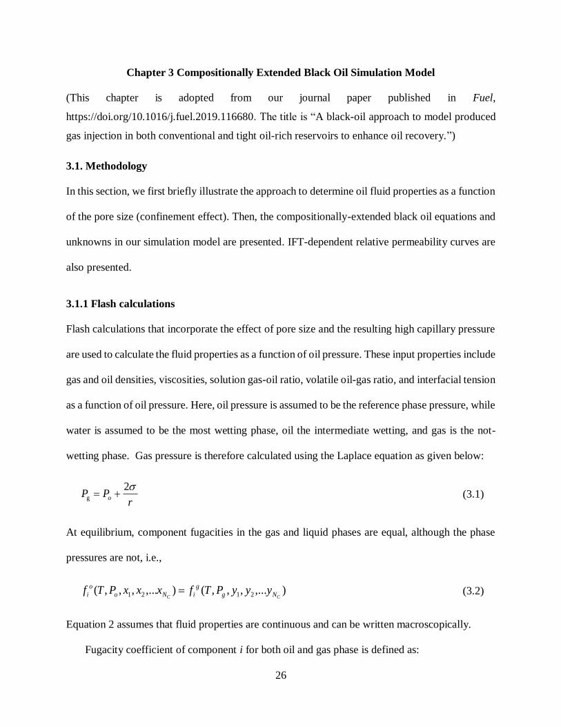
26

Chapter 3 Compositionally Extended Black Oil Simulation Model

(This chapter is adopted from our journal paper published in Fuel,

https://doi.org/10.1016/j.fuel.2019.116680. The title is “A black-oil approach to model produced

gas injection in both conventional and tight oil-rich reservoirs to enhance oil recovery.”)

3.1. Methodology

In this section, we first briefly illustrate the approach to determine oil fluid properties as a function

of the pore size (confinement effect). Then, the compositionally-extended black oil equations and

unknowns in our simulation model are presented. IFT-dependent relative permeability curves are

also presented.

3.1.1 Flash calculations

Flash calculations that incorporate the effect of pore size and the resulting high capillary pressure

are used to calculate the fluid properties as a function of oil pressure. These input properties include

gas and oil densities, viscosities, solution gas-oil ratio, volatile oil-gas ratio, and interfacial tension

as a function of oil pressure. Here, oil pressure is assumed to be the reference phase pressure, while

water is assumed to be the most wetting phase, oil the intermediate wetting, and gas is the not-

wetting phase. Gas pressure is therefore calculated using the Laplace equation as given below:

rPP o

2g (3.1)

At equilibrium, component fugacities in the gas and liquid phases are equal, although the phase

pressures are not, i.e.,

),...,,,(),...,,,( 2121 CC Ng

g

iNo

o

i yyyPTfxxxPTf (3.2)

Equation 2 assumes that fluid properties are continuous and can be written macroscopically.

Fugacity coefficient of component i for both oil and gas phase is defined as:

27

i

oo i

i o

f

x P (3.3a)

i

gg i

i g

f

y P (3.3b)

The equilibrium constant (Ki), defined as the /i i iK y x , in the successive substitution method

(SSM) is written as:

1

n no

gn n ii i g

i o

PfK K

f P

(3.4)

where n denotes the time step.

2

141 10on

i

gi i

f

f

(3.5)

Black oil properties above the original bubble-point pressure at different pore sizes are

estimated by adding small fractions of equilibrium gas composition at the current bubble-point

pressure to reach a new larger bubble-point pressure, until the critical point is achieved. Here, two

different approaches are used and compared, while extending the properties: using the same

bubble-point gas composition ( )old pZ r and equilibrium gas ( )old py r at infinitely large pore sizes

for varied effective pore sizes, i.e., Eq. 3.6, which was proposed in previous research (Nojabaei

and Johns, 2016); and using different bubble-point gas compositions at varied pore sizes (pr ), i.e.

Eq. 3.7. In the first approach, the overall compositions at different pores sizes are the same. In the

second approach, the overall composition is a function of pore size.

( ) (1 ) ( ) ( )new p old p old pZ r Z r y r . (3.6)

( ) (1 ) ( ) ( )new p old p old pZ r Z r y r . (3.7)

28

where Z is the overall composition, α is the selected dilution factor, and y is the equilibrium gas

composition at current bubble-point pressure. Smaller dilution factors yield more reliable

saturation pressures.

During primary depletion or gas injection, gas-oil interfacial tension changes with pressure and

reservoir fluid composition. Interfacial tension is calculated by using the Macleod and Sugden

correlation (developed by Macleoad (1923) and Sugden (1924), and modified for multicomponent

mixtures by Weinaug and Katz (1943); Pederson and Christensen (2007)) as a function of phase

composition and densities:

4

)(

cN

i

V

i

L

ii yx (3.8)

Using the Peng-Robinson cubic EoS (Peng and Robinson (1976)), we pre-calculate interfacial

tensions as a function of pressure and use this data as input to the simulator. Capillary pressure is

not only a function of IFT, but also pore size. The correlation among effective pore size, capillary

pressure, and saturation is derived from the Leverett J-function (Nojabaei et al. 2016). In this way,

fluid properties can be expressed as tabular functions of capillary pressure, saturation and pore

sizes.

3.1.2 Slim-tube simulation

To estimate MMPs by using the newly-proposed black oil fluid properties extrapolation approach,

slim-tube simulation is performed by injecting 1.0 PV (pore volume) produced gas into a 1-D slim-

tube with 100 grids saturated with Bakken oil. The black oil fluid properties of the pseudo-binary

mixture are pre-calculated. The dimensionless mass conservation equation for pseudo-component

i is expressed as:

29

0i i

D D

C F

t x

(3.9)

where iC is the volumetric composition of i and iF is the flux term.

1

pN

i ij i

j

C C S

(3.10)

1

pN

i ij i

j

F C f

(3.11)

The fractional flow is defined as:

1 1

/

/p p

j rj j

i N N

j rj j

j j

kf

k

(3.12)

3.1.3 Compositionally extended black oil model

In this study, our objective is to perform gas injection simulation for a variety of schemes in

conventional and tight oil-rich reservoir by using the compositionally-extended black oil model.

This black oil model is a special case of a standard compositional model with three components

(pseudo-oil, pseudo-gas, and water) and three phases (oleic, vapor, and aqueous). The fluid

properties as a function of pressure and pore-size dependent capillary pressure have been derived

from flash calculations prior to conducting simulation. We solve the following mass balance

equations for the principle unknowns of oil pressure Po, water saturation Sw, and overall pseudo-

gas mass composition Zg.

1 1 1

P P PN N Nrj

ij j j j ij j j ij

j j jj

kkP g z M S

t

(3.13)

30

where ij is the mass fraction of component i in phase j, and it is calculated as a function of

solution gas-oil ratio soR and volatile oil-gas ratio vR as described in a previous paper (Nojabaei et

al., 2016). Mij is the well mass flow term; and for water component we use the following equation:

w

www

ww

rw

B

S

tqP

B

kk

(3.14)

3.1.4 IFT-dependent relative permeability curves

We use the model by Coats (1980), that is a method to capture the effect of variable oil-gas IFT

changes on relative permeability curves by using a weighted sum of the base curve (immiscible

condition) relative permeability at capillary pressure-dominated flow and straight line (miscible

condition) relative permeability at viscous dominated flow. The weighting functions to calculate

gas and oil relative permeabilities are given below:

( ) 1 ( )gn

g grg rgcwk k f S f S (3.15)

( ) 1 ( )ogn

o orog rogcgk k f S f S (3.16)

1

g grg

wir gr

S SS

S S

(3.17)

1

1

g wir orgo

wir org

S S SS

S S

(3.18)

( )gr grS f S (3.19)

( )org orgS f S (3.20)

31

and

11/

( )

n

o

f

(3.21)

where gn

gS and ogn

oS are the base gas and oil relative permeability curves from experimental data

at immiscible conditions, gn and on are two tuning exponents to match with base curves; gS and

oS are two straight lines that represent relative permeabilities at miscible conditions; o is the

reference value of IFT corresponding to the base curves; and 1n is a tuning number in the range

of 4 to 10. We slightly modified the oil relative permeability by multiplying it by rogcgk (oil

relative permeability at connate gas saturation), as this term was absent in Coats’s method.

Correspondingly, oil relative permeability in three-phase condition is calculated by applying

Stones’ second method (Stone, 1973), i.e.,

( )( )ro rocw row rw rog rg rw rgk k k k k k k k . (3.22)

3.2 Bakken oil properties in nanopores

The pseudo-oil (dead oil) and pseudo-gas (surface gas) compositions were determined by

performing flash calculations at standard pressure and temperature. The pressure‒composition

diagrams of Bakken oil using two different gas adding approaches (Eq. 3.6 and Eq. 3.7) are shown

in Figure 3.1a and 3.1b, where Zg is the pseudo-gas composition. By using the same overall

compositions (at infinitely large pore sizes) for three different effective pore sizes (Eq. 3.6), the

critical point pressure or the first contact minimum miscibility pressure (MMP) converges at 4325

psia (in Figure 3.1a). Meanwhile, the oil and gas densities with pressure at three different pore

sizes converge at the critical point pressure, as shown in Figure 3.2a. By using different overall

32

compositions at different pore sizes (Eq. 3.7), the bubble-point curves of three pore sizes converge

at the pressure (P = 3689 psia at Zg = 0.34) lower than the critical point pressure.

Figure 3.1 Pressure‒composition plot for Bakken oil for three different effective pore sizes (a) by

using the same overall compositions at infinitely large pore sizes (Eq. 3.6) and (b) by using

different overall compositions at different pore sizes (Eq. 3.7).

The pseudo-oil densities at different pore sizes also converge at the same pressure, as shown in

Figure 3.2b.The stronger the nano-confinment is, the higher critical point pressure is achieved, i.e.,

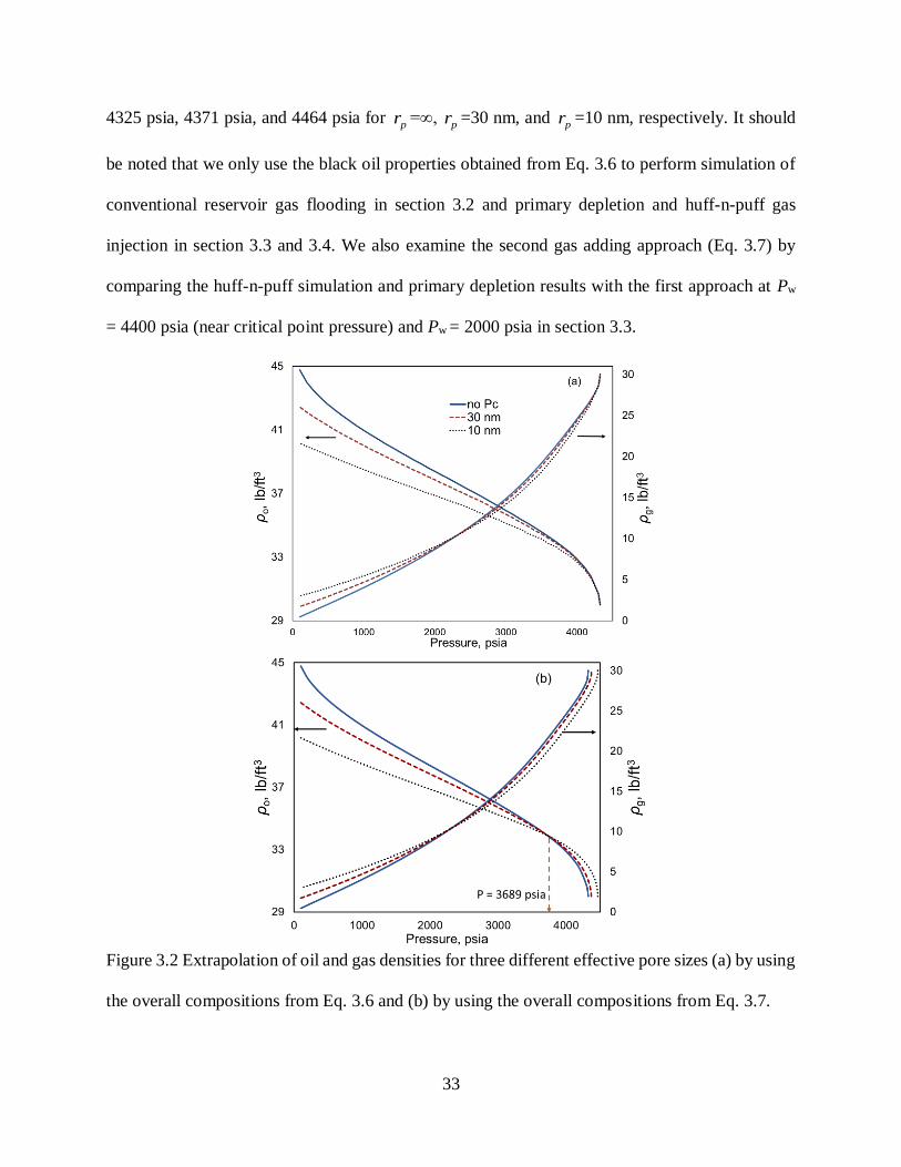
33

4325 psia, 4371 psia, and 4464 psia for pr =∞,

pr =30 nm, and pr =10 nm, respectively. It should

be noted that we only use the black oil properties obtained from Eq. 3.6 to perform simulation of

conventional reservoir gas flooding in section 3.2 and primary depletion and huff-n-puff gas

injection in section 3.3 and 3.4. We also examine the second gas adding approach (Eq. 3.7) by

comparing the huff-n-puff simulation and primary depletion results with the first approach at Pw

= 4400 psia (near critical point pressure) and Pw = 2000 psia in section 3.3.

Figure 3.2 Extrapolation of oil and gas densities for three different effective pore sizes (a) by using

the overall compositions from Eq. 3.6 and (b) by using the overall compositions from Eq. 3.7.

34

Figure 3.3a and b shows the oil component recovery as a function of pressure of 1.0 PVI by

using the extrapolated black oil properties obtained from Eq. 3.6 and from Eq. 3.7, and the turning

point of the curve to a horizontal line gives the MMP. The MMP by use of the first gas adding

approach (Eq. 3.6) is 4325 psia, while the second gas adding approach (Eq. 3.7), gives the MMPs

of 4325 psia, 4371 psia, and 4464 psia for pr =∞,

pr =30 nm, and pr =10 nm, respectively.

Figure 3.3 Oil component recovery as a function of pressure of 1.0 PVI by using the extrapolation

of black oil properties (a) getting from Eq. 3.6 and (b) from Eq. 3.7.

35

3.3 Miscible and immiscible gas flooding in conventional reservoir

The reservoir properties are tabulated in Table 3.1. The reservoir is a 2-D square domain with 225

(15 by 15) grid blocks. The reservoir fluid is Bakken oil with a bubble point pressure of Pb = 2860

psia at zero capillary pressure and reservoir temperature is 240 °F. The initial water saturation is

0.25.

Table 3.1 Reservoir and fluid properties for conventional reservoir.

Reservoir size, 2D 750 ft × 750 ft

Uniform matrix grid block size 50 ft × 50 ft

Matrix permeability 1000 md

Matrix porosity 10%

Reservoir thickness 10 ft

Fluid type Bakken fluid

Temperature 240 oF

For gas flooding, a homogeneous quarter of a five-spot pattern is used. The injector and

producer are located diagonally at the corner of the reservoir domain. The injected gas is surface

gas, which is also defined as the composition of the pseudo-gas component (see Nojabaei and

Johns (2016)). Gas floods at three different initial reservoir pressures of Pi = 2500, 3000, and 4500

psia are simulated. The corresponding bottomhole pressures for the production wells are 100 psi

lower than the initial reservoir pressures, i.e., Pw = 2400, 2900, and 4400 psia. The surface gas is

injected continuously from time zero with a constant injection rate of 1000 Mscf/day. The total

production time is 560 days and the cumulative oil recoveries from the compositionally-extended

black oil model are plotted in Figure 3.4.

At Pi = 2500 psia and Pw = 2400 psia, the reservoir is initially saturated (Pi < Pb) and the injected

gas displaces the oil immiscibly. Gas break-through occurs early at 12.8 days, which corresponds

to 0.14 PVI (pore volume injected). At Pi = 3000 psia and Pw = 2900 psia, the reservoir is initially

undersaturated (Pi > Pb) and the gas flood remains immiscible, and gas break-through occurs at

36

26.1 days (PVI = 0.23), slightly later than the previous case. At Pi = 4500 psia and Pw = 4400 psia,

the reservoir is initially undersaturated (Pi >Pb) and the gas flood is miscible because the BHP is

larger than the critical pressure or MMP. Gas break-through occurs at 51.1 days, which

corresponds to 0.25 PVI. By comparing the cumulative oil recovery curves, it is observed that

before gas breaks through, the oil recovery rate is the same for three scenarios regardless of being

miscible or immiscible. After gas breaks through, immiscible flooding at higher pressures results

in a larger oil recovery rate. Additionally, miscible flooding maintains a constant high recovery

rate and reaches the maximum recovery in a shorter period of time.

Figure 3.4 Cumulative oil production of gas floods at different initial reservoir pressures and

production pressures.

The gas composition in the production well block for the three scenarios are shown in Figure

3.5. For the case of Pi = 2500 psia, Zg is initially the same as the original pseudo-gas composition

at 0.25. As gas is injected and breaks-through the production well, the pseudo-gas composition

increases gradually while the reservoir fluid remains in the two-phase region. At later time the gas

composition suddenly increases to 1.0, showing that oil has been completely vaporized. For Pi =

37

3000 psia, the increase is similar to the previous case although the two-phase period is shorter. For

Pi = 4500 psia, there is no two-phase period as this corresponds to a completely miscible first-

contact flood, i.e. above the MMP and flow would be piston-like with a very sharp front if more

grid blocks had been used. Numerical dispersion is smearing this front since there is no self-

sharpening behavior above the MMP.

Figure 3.5 Gas composition at production well block for gas injection in conventional reservoirs

at different initial reservoir pressures and production pressures.

The distribution of gas saturation at different displacing times for cases of Pi = 3000 psia and

Pw = 2900 psia, and Pi = 4500 psia and Pw = 4400 psia (first-contact miscible flooding) are plotted

in Figures 3.6 and 3.7, respectively. For the lower pressure case, the gas saturation increases at the

production well after 30 days. The two-phase (oil-gas) region appears near time zero, and

propagates throughout the entire reservoir for continous gas injection. At later time, oil saturation

at both injection and production well is zero. However, for the misicible flood case, the

dispalcement is piston-like. A distinct single displacing front is clearly observed from the

38

beginning of the simulation to the end. Mobile oil in the reservoir is completely recovered in 150

days, which is also verified by the cumulative oil recovery curve in Figure 3.7.

Figure 3.6 Gas saturation distribution in the conventional reservoir at different times (Pi=3000 psia

and Pw =2900 psia).

Figure 3.7 Gas saturation distribution in the conventional reservoir at different times (Pi=4500 psia

and Pw =4400 psia).

3.4 Huff-n-puff in an oil-rich tight reservoir

For this case, the reservoir size and fluid properties are the same as case 1 (given in Table 3.1).

However, reservoir permeability for case 2 is different, which will be discussed next. The reservoir

39

fluid is Bakken oil with a bubble point pressure of Pb = 2860 psia when capillary pressure is zero

and Pb = 2750 psia when capillary pressure in flash calculations is taken into account and pore size

is 15 nm. The initial reservoir pressure is 5000 psia and the initial water saturation is 0.15. Middle

Bakken, the formation considered here, is not ultra-tight, but only tight (permeability about 0.05

md).

Table 3.2 Reservoir and fluid properties for tight oil-rich reservoir.

Reservoir size, 2D 750 ft × 750 ft

Uniform matrix grid block size 50 ft × 50 ft

Matrix porosity 10%

Reservoir thickness 10 ft

Fluid type Bakken fluid

Initial reservoir pressure 5000 psia

Temperature 240oF

Instead of creating hydraulic fractures, we increase the matrix permeability near the production

well to account for the effect of increased conductivity in the reservoir caused by fractures. The

reservoir permeability map and the location of the horizontal well are shown in Figure 3.8. The

increased permeability changes the physics to completely advection-dominated mass transfer. For

the Middle Bakken, as the formation is not ultra-tight, mass transfer is likely advection-dominated

anyway, and diffusion should play a small role.

40

Figure 3.8 Reservoir permeability map for tight oil-rich reservoir.

In this section, we consider four BHPs at Pw = 1000, 2000, 3000, and 4000 psia to study the

production performances for both primary depletion and huff-n-puff gas injection schemes. For

the huff-n-puff gas injection, after producing for 50 days through primary depletion, produced gas

(surface gas) is injected at constant rate of 25 Mscf for 30 days, followed by a 20-day soaking

period. For all schemes, the total production time is 800 days. Unlike conventional reservoirs,

nano-pore size-induced large capillary pressure in tight formations strongly affects the fluid phase

behavior (2013), and may further affect the oil recovery prediction. In order to investigate the

capillary pressure effect on production performance, we design three scenarios: without capillary

pressure in flow and flash calculations, with capillary pressure in flow but without capillary

pressure in flash calculations, and with capillary pressure both in flow and flash calculations. We

considered an average pore size of 15nm for the cases that capillary pressure influences flash

calculations. To incorporate the effect of capillary pressure on fluid properties through flash

calculations, we multiplied the interfacial tension calculated by using Mcleod and Sugden

correlation by a factor of three, as the calculated interfacial tensions are underestimated as stated

41

by Nojabaei et al. (2013). We perform the primary and huff-n-puff gas injection schemes at four

different BHPs under three different scenarios. All the simulation results are plotted in Figure

3.9a–c. The corresponding oil pressure at the well block at different times are plotted in Figure

3.10.

42

Figure 3.9 Cumulative oil recovery for primary depletion and huff-n-puff gas injection with and

without considering capillary pressure in tight oil-rich reservoirs at at Pi=5000 psia and (a) Pw

=1000 psia, (b) Pw =2000 psia, (c) Pw =3000 psia, 4000 psia, and 4400 psia.

Figure 3.10 Oil pressure at the well block for primary depletion and huff-n-puff gas injection with

and without considering capillary pressure in tight oil-rich reservoirs at Pi=5000 psia and Pw=1000,

2000, 3000, 4000, and 4500 psia, respectively.

43

It can be seen from Figure 3.9a–c that a lower BHP contributes to a higher cumulative oil

recovery for both primary depletion and huff-n-puff gas injection schemes. This is because a larger

pressure difference between the reservoir pressure and BHP is beneficial for fluid flow.

Furthermore, cumulative oil recoveries for primary depletion without considering capillary

pressure at Pw = 1000 and 2000 psia are around 8000 STB, which is 1-2 times larger than 2800

STB at Pw = 3000 psia and 4-5 times larger than 1400 STB at Pw = 4000 psia. The large recovery

at the lower BHPs is also owing to the effective solution gas drive, while the dissolved gas releases

from oil for reservoir pressures below the bubble point pressure (2860 psia). Comparing the

cumulative oil production of primary depletion to huff-n-puff gas injection scheme at the same

BHP, it is observed that when the production pressure (Pw = 1000 and 2000 psia) is below bubble

point pressure, both schemes achieve almost the same final oil recovery. However, when the

production bottomhole pressures (Pw = 3000, 4000, and 4500 psia) are above bubble point

pressure, huff-n-puff results in a larger final oil recovery compared to primary depletion with an

increase of 7.22%, 12.86%, and 26.75%, respectively. This is because huff-n-puff gas injection is

more efficient at miscible or near-miscible conditions (also concluded by Song and Yang (2017)).

The viscosity and interfacial tension of original oil could be effectively reduced as gas is dissolved

in oil; meanwhile, the swollen diluted-oil is easy to be displaced and recovered (Du et al., 2019).

From previous research, we know that large gas-oil capillary pressure due to the nano-

confinement significantly affects the recovery performance (Nojabaei et al., 2016). The results in

Figure 3.9a–c indicate that inclusion of capillary pressure in flash could significantly increase oil

recovery at a lower BHP (Pw = 1000 psia). However, when BHP pressure is increased, the impact

of capillary pressure in flash on oil recovery weakens and almost disappears at Pw = 4000 psia.

The reason is that the IFT between oil and gas phases reduces as the reservoir pressure increases

44

and becomes zero at MMP (4325 psia), resulting in a diminished capillary pressure. Nevertheless,

inclusion of capillary pressure in flow does not contribute to oil recovery at higher BHPs and even

decreases the recovery to a small extend at a lower BHP. Inclusion of capillary pressure in flash

calculation influences primary recoveries for lower pressure cases, however, it doesn’t influence

the enhanced oil recovery as gas injection enhances recoveries only at higher pressures where the

effect of capillary pressure becomes negligible.

Here, we also plot the cumulative gas recoveries for primary depletion and huff-n-puff gas

injection for the case with capillary pressure in both flow and flash at five different BHPs, as shown

in Figure 3.11. This plot indicates that the cumulative produced gas for huff-n-puff is always higher

than that for primary depletion. The total injected gas in the huff period is 750 Mscf. The enhanced

cumulative gas recoveries for Pw = 1000, 2000, 3000, 4000 and 4500 psia are 508, 570, 485, 390,

and 389 Mscf, respectively. Most of the injected gas is produced for lower pressures (Pw = 1000

and 2000 psia) (production is still going on). It can be concluded that if gas is injected when

reservoir is already saturated (Pw = 1000 and 2000 psia), the injected gas will flow back with oil

instead of dissolving into crude oil and increasing the oil recovery. However, when the reservoir

pressure is at miscible or near-miscible condition (Pw = 3000, 4000 and 4500 psia), most of the

injected gas dissolves into the crude oil and improves the oil recovery.

45

Figure 3.11 Cumulative gas recovery for primary depletion and huff-n-puff gas injection at Pw =

1000, 2000, 3000, 4000, and 4500 psia, respectively accounting for the capillary pressure both in

flow and flash.

In this section, we also examine the second gas adding approach (Eq. 3.7) by comparing the

huff-n-puff gas injection with the first approach (Eq. 3.6) at production pressure of Pw = 4400 psia

(near critical point pressure) and Pw = 2000 psia. The results are tabulated in Table 3.3. Adopting

different black oil properties by using different gas adding approaches would make a difference

on recovery when Pc in both flash and flow is included, although the difference is not significant.

A decrease in recovery is observed at a higher production pressure (4400 psia) and an increase in

recovery is observed at a lower pressure by using second approach owing to the black oil properties

distortion below and above P = 3689 psia.

Table 3.3 Gas production of huff-n-puff at Pw = 4400 psia and 2000 psia using two different gas

adding approaches.

46

Pw (psia)

Pc in flow Pc in flash

Huff-n-huff

Production/Mscf

(using Eq. 3.6)

Production/Mscf

(using Eq. 3.7)

4400 Yes Yes 1048.25 1047.53

2000 Yes Yes 9122.98 9132.59

3.5 Effect of IFT-dependent relative permeability on recovery

IFT-dependent oil-gas relative permeability data that accounts for the pressure and

compositional change are incorporated in this compositionally-extended simulation model.

Simulation studies are performed in a tight oil-rich reservoir (the reservoir model of Case 2 is used)

to examine the effect of dynamic relative permeability on recovery in primary production and huff-

n-puff gas injection schemes. The initial reservoir pressure is 5000 psia and the BHPs are set to be

2000, 3000, and 4000 psia, respectively and the simulation results are compared to those with fixed

base relative permeability curves. According to Coats’s method, base gas and oil relative

permeability curves from experimental data at immiscible conditions are required. In this study,

the base relative permeability curves for the Bakken reservoir are adopted from Yu et al. (2014)

as shown in Figure 3.12. The IFT-dependent relative permeability curves are then calculated using

weighted base (immiscible) relative permeability curves and weighted straight line (miscible)

relative permeability curves (dotted line in Figure 3.12). The IFT change with composition is pre-

calculated as a function of pressure and the data are plotted in Figure 3.13. We assume that the

reference value of IFT ( o in Eq. 3.21), corresponding to the base oil-gas relative permeability

curves, is 4.736 dyne/cm (at 2000 psia).

47

Figure 3.12 Relative permeability curves for case 3, adopted from Yu et al. (2014).

Figure 3.13 Oil-gas IFTs of Bakken black oil at different reservoir pressures.

The oil recovery simulation results for primary depletion and huff-n-puff gas injection schemes

at different BHPs are plotted in Figure 3.14a–c. It should be noted that for all the curves, capillary

pressure in both flow and flash calculations are included. At a lower BHP (Pw = 2000 psia), an

obvious increase in the cumulative oil recovery is observed for both primary and huff-n-puff gas

48

injection schemes when the IFT-dependent relative permeability curves are used in the simulation

model. However, at higher BHPs (Pw = 3000 and 4000 psia), no distinct change in oil recovery is

observed compared to the base relative permeability case. The reason is that for the primary

depletion schemes, only single phase oil exists at high BHPs (Pw > Pb) and IFT is not defined.

Therefore, fluid flow in reservoir is exactly the same as the case using base relative permeability

curves. For the huff-n-puff gas injection schemes, in spite that a small fraction of injected gas

appears near the production well, oil saturation is still very high and oil phase flow is dominant in

the reservoir. It can be concluded that IFT-dependent relative permeability significantly impacts

oil recovery only for a reservoir with a dominant mobile oil-gas two-phase region.

49

Figure 3.14 Cumulative oil production for huff-n-puff gas injection in tight oil-rich reservoirs

using IFT-dependent relative permeability curves and base relative permeability curves,

respectively, at Pi=5000 psia and (a) Pw =2000 psia, (b) Pw =3000 psia, and (c) Pw =4000 psia.

50

Chapter 4 Diffusion Coefficient with Nano-confinement Effects

(This chapter of the dissertation is adopted from our published paper in the Journal of Petroleum

Science Engineering, https://doi.org/10.1016/j.petrol.2020.107362. The title is “Estimating

diffusion coefficients of shale oil, gas, and condensate with nano-confinement effect”)

4.1 Methodology

Sigmund correlation is one of the most extensively used correlations to calculate diffusion

coefficients; however, the unit systems used were not well documented and varied in different

studies (Nghiem et al., 2001; Yu et al., 2015; Alharthy et al., 2018). Applying Sigmund correlation

with uncertain units may result in incorrect diffusivities. For example, one simulation work

(Alharthy et al., 2018) used Sigmund correlation and tried to match the calculated diffusion

coefficients with the experimental data selected from Sigmund’s paper but the results were

unsatisfactory (underestimated diffusivities by one or two orders). Here, Sigmund correlation

(Sigmund, 1976a; 1976b) and complementary formulas by later researchers (da Silva and

Belery,1989; Reid et al., 1987) are summarized. The definitions of parameters with the appropriate

units are given in the “Nomenclature” section. According to Sigmund correlation, the binary

diffusion coefficient, ijD, between components i and j, is calculated as:

0 0

2 30.99589 0.096016 0.22035 0.032874k ij

ij kr kr kr

k

DD

(4.1)

da Silva and Belery (1989) claimed that Eq. 4.1 gave a negative ijD at 3.7kr and suggested

to use the following expression for 3.7kr :

0 0

0.18839exp(3 )k ij

ij kr

k

DD

(4.2)

51

0 0

k ijD is the zero pressure limit of the density-diffusion coefficient product in phase k,

calculated by:

1/21/2

0 0

2

0.0018583 1 1k ij

ij ij i j

TD

R M M

(4.3)

5/3

1

2/3

1

c

c

n

ik ciikr k n

ik cii

y v

y v

(4.4)

where, ij is the Lennard Jones size parameter (collision diameter), and

ij is the collision integral

of the Lennard-Jones potential, both are associated with the component critical properties (Reid et

al., 1987):

2

i j

ij

(4.5)

ij i j (4.6)

1/3

(2.3551 0.087 ) cii i

ci

T

P

(4.7)

(0.7915 0.1963 )i B i cik T (4.8)

0.15610

1.06036 0.19300 1.03587 1.76474

( ) exp(0.47635 ) exp(1.52996 ) exp(3.89411 )ij

ij ij ij ijT T T T (4.9)

Bij

ij

kT T

(4.10)

where Bk is the Boltzmann’s constant (=1.3805E-16 ergs/K) and ij is the characteristic Lennard-

Jones energy.

Sigmund (1976b) also defined the diffusion coefficient of component i in phase k of a

multicomponent mixture based on Wilke formula (Wilke, 1950), as given in Eq. 4.11.

52

1 ikik

jk

i jij

yD

y

D

(4.11)

In Wilke‒Chang correlation (Wilke and Chang, 1955), the diffusion coefficient of component

i in phase k in mixture, is expressed as:

8 1/2

0.6

7.4 10 ( )ikik

k bi

M TD

v

(4.12)

with

1

jk jj i

ik

jk

y MM

y

(4.13)

where biv is the partial molar volume of component i at the boiling point and is calculated as:

1.0480.285bi cv v (4.14)

Hayduk and Minhas (1982) proposed three empirical correlations for water, n-paraffins (C5 to

C32), and nonaqueous mixtures as the solutes, respectively. In this study, the correlations for

nonaqueous mixtures (Eq. 4.15) and for n-paraffins (Eq. 4.18) are used to predict the diffusivities

in gas or oil phase.

8 1.29 0.5

0.92 0.23 0.42

1.55 10 ( )

( )

ikik

k ik i

T PD

v P

(4.15)

with

1

jk jj i

ik

ik

y PP

y

(4.16)

1

jk bjj i

ik

ik

y vv

y

(4.17)

where jP is the parachor of component j.

53

0.791(10.2/ )8 1.47

0.71

1.33 10

( )

bi

kik

bi

TD

v

(4.18)

4.2 Validation of empirical correlations

First, we apply the three empirical correlations (Wilke‒Chang, Hayduk–Minhas, and Sigmund) to

calculate diffusion coefficients and compare them with the laboratory measurements, aiming at

screening out the correlations that are suitable for shale fluids at reservoir conditions. Here,

experimental data for two mixtures at high pressures are selected from the literature, i.e., C1/C3

mixture (Sigmund 1976a) and C1/C10 mixture (Dysthe and Hafskjold, 1995). The first set (C1/C3

mixture) contains light hydrocarbons, with similar properties as shale gas and condensate. The

second set (C1/C10 mixture) is light hydrocarbon in decane, similar to a mixture of injected gas in

crude oil. The experimental data and fitting curves are plotted in Figures 4.1 and 4.2.

54

Figure 4.1 The diffusion coefficient of CH4 in C1/C3 mixtures by using empirical correlations and

comparison with experimental data (Sigmund, 1976a) at (a) 160 °F and 3000 psia; (b) 160 °F and

2000 psia; (c) 100 °F and 2000 psia; (d) 220 °F and 1000 psia.

55

Figure 4.2 The diffusion coefficient of CH4 in C1/C10 mixtures by using empirical correlations and

comparison with experimental data (Dysthe and Hafskjold, 1995) at (a) 86 °F and 40 MPa; (b)

86 °F and 50 MPa.

In Figure 4.1, diffusion coefficients are calculated and compared to the four groups of

measurements for the C1/C3 mixture at high pressures and temperatures sets: (a) 160 °F and 3000

psia, (b) 160 °F and 2000 psia, (c) 100 °F and 2000 psia, and (d) 220 °F and 1000 psia. As was

expected, employing Sigmund correlation always resulted in a good match at different pressures,

considering that Sigmund used these experimental data to develop the correlation. Wilke‒Chang

56

and Hayduk‒Minhas correlations for nonaqueous mixtures (Eq. 4.15) overestimate the

diffusivities at high pressures (2000 and 3000 psia), but underestimate the diffusivities at relatively

lower pressure of 1000 psia. Hayduk‒Minhas correlation for n-paraffins (Eq. 4.18) underestimate

the diffusivities at all given pressures. In Figure 4.2, two groups of calculations and comparisons

were performed for C1/C10 mixture at following high pressures: (a) 86 °F and 40 MPa and (b) 86

°F and 50 MPa. Sigmund correlation is still superior to the other three correlations and offers the

best fitting. One reason to explain the unsatisfactory prediction of diffusivity using Wilke‒Chang

and Hayduk‒Minhas correlations is that these correlations were derived from and suitable for low-

pressure liquid systems. Based on the validation results, Sigmund correlation is selected to predict

the diffusivities in shale gas and liquid systems in the following sections.

4.3 Diffusivity of shale fluids without confinement effects

The compositions of Marcellus shale gas (Bullin et al., 2008), Lower Huron shale gas, Marcellus

shale condensate (Elamin, 2013), and Bakken shale oil (Nojabaei and Johns, 2016) are given in

Table 4.1. The corresponding reservoir temperatures are 140 °F, 110 °F, 150 °F, and 240 °F,

respectively.

Table 4.1 Compositions of Marcellus shale gas, Lower Huron shale gas, Marcellus shale

condensate, and Bakken shale oil (unit: mole fraction).

Marcellus Shale Gas

CO2 C1 C2 C3 N2

0.003 0.955 0.03 0.01 0.002

Lower Huron Shale Gas

CO2 C1 C2 C3 N2

0.0023 0.972 0.0153 0.0004 0.01

Marcellus Shale Condensate

CO2 N2 C1 C2 C3 IC4 NC4 IC5 NC5 C6 C7

0.0124 0.0034 0.7967 0.0547 0.0396 0.011 0.0152 0.0079 0.0063 0.0113 0.0415

Bakken Shale Oil

C1 C2 C3 C4 C5C6 C7C12 C13C21 C22C80

57

0.36736 0.14885 0.09334 0.05751 0.06406 0.15854 0.0733 0.03704

Sigmund correlation is used to calculate the diffusivities of three types of shale fluids at

reservoir temperatures. For Marcellus shale gas (Figure 4.3), the diffusivity is decreased

dramatically with increasing pressure at lower pressures, but the decline reaches a plateau at higher

pressures. Lighter components have relatively higher diffusivities compared to heavier

components.

Figure 4.3 The diffusivities of components of Marcellus shale gas in gas phase at the reservoir

temperature.

For Marcellus shale condensate, the diffusivities of CO2, CH4, and n-C4H10 in gas and liquid

phases are plotted in one figure (Figure 4.4). At lower pressures, the diffusivities of components

in gas phase are larger than in liquid phase by almost one order of magnitude. For example, at

1500 psia, the diffusivity of CH4 in gas phase is 1.17×10-3 cm2/s and in liquid phase, it is 1.00×10-

4 cm2/s. As pressure increases, the diffusivities in gas phase decline dramatically. Meanwhile, the

diffusivities in liquid phase increase smoothly and converge to diffusivities in gas phase with a

58

sudden rise at P = 2570 psia. This is because the liquid phase disappears at the dew-point pressure.

Above the dew-point pressure, the diffusivities in gas phase keep decreasing slowly with pressure.

Figure 4.4 The diffusivities of components of Marcellus shale condensate in gas and liquid phases

at the reservoir temperature.

For Bakken shale oil, the diffusivities of all components in gas phase are plotted in Figure 4.5a.

Similar to Marcellus shale gas, lighter components yield a higher diffusivity. At 1000 psia, the

diffusivity of CH4 in gas phase is almost one order lager than that of C22C80. As pressure increases,

the diffusivities decrease and the gap between light and heavier components is narrowed. In the

liquid phase (Figure 4.5b), the diffusivities are decreasing slightly with pressure, which is opposite

to the case in shale condensate. After reaching bubble-point pressure (Pb = 2860 psia), an almost

linear declining of diffusivities with pressure is observed. Comparing Figure 4.5a and 4.5b, the

diffusivities in gas phase are almost two orders larger than in liquid phase at the same pressure.

59

Figure 4.5 The diffusivities of components in (a) Bakken oil in gas phase and (b) Bakken oil in

liquid phase at reservoir temperatures.

60

4.4 Nano-confinement effects on diffusivity

In this section, two methods are introduced to consider the nano-confinement effects, i.e., critical

property shift and large gas-oil capillary pressure. Both methods can alter the phase properties in

the nano-pores with their specific performance.

4.4.1 Critical Property Shift

Morishige et al. (1997) observed a significant reduction in critical temperature of argon nitrogen,

oxygen, ethylene, and CO2 in nano-scale porous materials. Zarragoicoechea and Kuz (2004)

developed a model to account for the critical temperature shift based on van der Waals equation

of state (Eq. 4.19) and reported a good match with the experimental data by Morishige et al. (1997).

They also developed an equation for the critical pressure shift (Eq. 4.20), even though the equation

has not been experimentally verified owing to the difficulty in operation (Zarragoicoechea and

Kuz, 2004).

2

0.9409 0.2415c cp ij ij

c

c p p

T TT

T r r

(4.19)

2

0.9409 0.2415c cp ij ij

c

c p p

P PP

P r r

(4.20)

30.244 cij

c

T

P (4.21)

where cT and cP are the bulk critical temperature and pressure, and cpT and

cpP are the pore critical

temperature and pressure, respectively.

61

4.4.2 Gas-oil Capillary pressure

Owing to the large gas-oil capillary pressure in nano-sized pores, there is a phase pressure

difference in as oil and gas phases co-exist. Gas pressure is calculated using the Laplace equation

as given below:

g

2o

p

P Pr

(4.22)

where, is the interfacial tension (IFT) between oil and gas phases and is calculated by using the

Macleod and Sugden correlation (developed by Macleoad, 1923, and Sugden, 1924, and modified

for multicomponent mixtures by Weinaug and Katz, 1943; Pedersen and Christensen, 2007) as a

function of phase composition and densities:

4

)(

cN

i

V

i

L

ii yx (4.23)

At equilibrium, component fugacities in the gas and liquid phases are equal, although the phase

pressures are not, i.e.,

),...,,,(),...,,,( 2121 CC Ng

g

iNo

o

i yyyPTfxxxPTf . (4.24)

4.4.3 Nano-confinement effects on diffusivity

62

Figure 4.6 P–T phase envelops of Bakken shale oil, Bakken shale oil with CO2 injection at 20%

and 50%, Marcellus shale condensate, condensate with CO2 injection at 20%, 50% and 80%, and

Marcellus shale gas.

For Marcellus shale gas, the reservoir fluid is only single gas phase at the reservoir temperature,

as shown in Figure 4.6. The gas-oil capillary pressure is zero and only the critical property shifts

nano-confinement effect is taken into consideration. The diffusivities of CO2 and CH4 in gas phase

at variable CO2 mole percentage and at different pressures and pore sizes are plotted in Figure 4.7a

and b. Both CO2 and CH4 diffusivities in gas phase decrease slightly with continuous CO2 injection.

Lower pressure yields a higher diffusivity. At higher pressures, the declining of diffusivity with

pressure slows down. Including critical property shifts could increase the diffusion coefficients;

the smaller the pore size is, the more significant the effect is. For example, at 80% CO2 mole

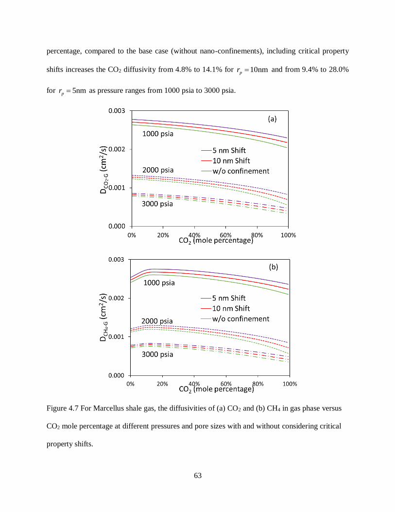
63

percentage, compared to the base case (without nano-confinements), including critical property

shifts increases the CO2 diffusivity from 4.8% to 14.1% for 10nmpr and from 9.4% to 28.0%

for 5nmpr as pressure ranges from 1000 psia to 3000 psia.

Figure 4.7 For Marcellus shale gas, the diffusivities of (a) CO2 and (b) CH4 in gas phase versus

CO2 mole percentage at different pressures and pore sizes with and without considering critical

property shifts.

64

Here, we calculate the diffusivity of N2 and CH4 for Lower Huron shale gas at varied N2 mole

percentage to examine the diffusion behavior when nitrogen is used as the fracking fluid, and the

results are plotted in Figure 4.8a and b. It should be noted that we also calculated the diffusivity

of CO2 and CH4 for Lower Huron shale gas at varied CO2 mole percentage, but the results are not

showing here because the data are very close to but only slightly smaller than those in Marcellus

shale gas (Figure 7a and b) due to its lower reservoir temperature. Comparing Figure 4.7a and b to

Figure 4.8a and b, it is found that the diffusivities of N2 and CH4 increases with N2 concentration,

in contrast with the diffusivities of CO2 and CH4 in CO2 environment. This is because that the

molar density of shale gas is increased with continuous injection of CO2 (Figure 4.9a), but is

declined with an increase in N2 concentration, as shown in (Figure 4.9b). In addition, including

critical property shifts reduces the molar density (Figure 4.9a and b), resulting in an increased

diffusivity for both CO2 and N2 cases.

65

Figure 4.8 For Lower Huron, the diffusivities of (a) N2 and (b) CH4 in gas phase versus N2 mole

percentage at different pressures and pore sizes with and without considering critical property

shifts.

66

Figure 4.9 The gas molar density of (a) Marcellus shale gas versus CO2 mole percentage and (b)

Lower Huron shale gas versus N2 mole percentage at different pressures and pore sizes with and

without considering critical property shifts.

For Marcellus shale condensate, CO2 diffusivities in gas phase at variable CO2 percentage with

and without nano-confinements are plotted in Figure 4.10, including (a) P = 1000 psia, 30nmpr

; (b) P = 1000 psia, 15nmpr ; (c) P = 3000 psia, 30nmpr ; and (d) P = 3000 psia, 15nmpr .

At 1000 psia (Figure 10a and b), compared with the base case, including critical property shifts

decreases the diffusivity in gas phase at CO2 percentage lower than 50% (two phases co-exist in

the system), but increases the diffusivities in gas phase at CO2 percentage larger than 60% (single

gas phase exists in the system). The smaller the pore size is, the stronger the effect becomes; for

example, at 40% CO2, including critical property shifts reduces the CO2 diffusivity about 1.0%

and 2.3% at 30nmpr and 15 nm respectively. At 80% CO2, including critical property shifts

increases the CO2 diffusivity about 1.9% and 3.8% at 30nmpr and 15 nm, respectively. The gas-

67

oil capillary pressure, as another nano-confinement effect, exists only in a two-phase system. In

this study, the interfacial tension is increased by three times (multiplying Eq. 4.23 by three) based

on a previous study (Ayirala and Rao, 2006) indicating that measured IFTs were two or three times

larger than those from Macleod and Sugden correlation (Eq. 4.23). As shown in Figure 10a and

b, including gas-oil capillary pressure effect alters the diffusion behaviors by decreasing the

diffusivities before in the two phase region (at CO2 <80% for 30nmpr and 70% for 15nmpr )

and after the single gas phase appears, its influence on diffusivity diminishes. Again, the smaller

the pore size is, the more significant the effect is; for example, at 40% of CO2, including gas-oil

capillary pressure effect reduces the CO2 diffusivity about 13.1% and 19.1% at 30nmpr and 15

nm, respectively. When both effects are incorporated, capillary pressure effect is more pronounced

compared to the critical property shifts.

68

Figure 4.10 For Marcellus shale condensate, the diffusivities of CO2 in gas phase versus CO2 mole

percentage at different pressures and pore sizes with and without considering nano-confinement

effects.

69

For Bakken shale oil, Figure 4.11 shows the oil with and without nano-confinement effect

(capillary pressure, critical property shifts) at pore size of 10 nm. Including capillary pressure

effect reduces the bubble-point-pressure curve but slightly increases the dew-point-pressure curve.

The entire phase envelope shrinks if the critical property shifts is considered and the shrinkage

becomes severer at higher temperatures.

Figure 4.11 Original Bakken oil with and without nano-confinement effect (capillary pressure,

critical property shifts) at pore size of 10 nm.

The diffusivities of CO2 and C5C6 in gas phase versus CO2 mole percentage at 1500 psia and

10nmpr with and without nano-confinement effects are plotted in Figure 4.12a and b. Including

capillary pressure effect reduces the diffusivity of CO2 and C5C6 in gas phase, by 16.2% and 17.4%

at 40% CO2. Including critical property shifts reduces the diffusivity of CO2 and C5C6 at lower

CO2 percentage slightly, and increases the diffusivity of C5C6 at higher CO2 percentage. When

70

both effects are included, the effect of capillary pressure to reduce the diffusivity in gas phase is

dominant.

Figure 4.12 For Bakken shale oil, the diffusivities of (a) CO2 and (b) C5C6 in gas phase versus CO2

mole percentage at 1500 psia and at pore size of 10 nm with and without considering nano-

confinement effects.

The diffusivities of CO2 and C5C6 in liquid phase versus CO2 mole percentage at 10nmpr

with and without nano-confinement effects are plotted in Figure 4.13, including (a) CO2 at 1500

71

psia, (b) C5C6 at 1500 psia, (c) CO2 at 3000 psia, and (d) C5C6 at 3000 psia. At a lower pressure

i.e., 1500 psia, gas-oil capillary pressure effect decreases the diffusivities with an increase in CO2

percentage, whereas, critical property shifts increase the diffusivities with a decrease in CO2

percentage. At a higher pressure, i.e., 3000 psia, both capillary pressure effect and critical property

shifts increase the diffusivities in liquid phase. A combination of both confinement effects

increases the diffusivities in liquid phase by 25% at lower CO2 percentage, but this effect

diminishes with continuous CO2 injection.

72

Figure 4.13 For Bakken shale oil, the diffusivities of CO2 and C5C6 in liquid phase versus CO2

mole percentage at at pore size of 10 nm with and without considering nano-confinement effects,

including (a) CO2 at 1500 psia; (b) C5C6 at 1500 psia; (c) CO2 at 3000 psia; and (d) C5C6 at 3000

psia.

4.4.3 Diffusion with confinement effect on shale oil production

As discussed in section 4.4.3, the confinement effect will affect the diffusion coefficient in

nano-pore shale reservoirs. In this section, we will examine the diffusion with confinement effect

73

on Bakken shale oil production during huff-n-puff produced gas injection process. The

permeability of the shale matrix is shown in Figure 4.14.

Figure 4.14 Reservoir permeability map for tight oil-rich reservoir.

Figure 4.15 Cumulative oil production of primary depletion and huff-n-puff gas injection with and

without molecular diffusion.

The gas is injected at constant injection rate of 10 Mscf/day. Two circles of huff-n-puff is

performed, including 55 days of gas injection and 37 days of soaking period for each circle. First,

we examine the molecular diffusion effect on oil production. The cumulative oil production of

primary depletion and huff-n-puff gas injection with and without molecular diffusion are plotted

74

in Figure 4.15. The results show that using huff-n-puff gas injection approach could increase the

oil production by 11.91%. Moreover, inclusion of molecular diffusion effect could increase the oil

production by almost 2% compared to one without including molecular diffusion effect.

Figure 4.16 Reservoir permeability map for tight oil-rich reservoir.

We also examine the diffusion with confinement effect on production behavior. The results are

plotted in Figure 4.16. It shows that including huff-n-puff could slight increase the oil production

during the huff-n-puff process but decrease oil production at a later time. Overall, the effect is not

very significant.

4.5 Effective Diffusion Coefficient in Porous Media

4.5.1 Methodology

An effective diffusion coefficient is suggested to characterize the diffusion behavior in a porous

media by the following expression (Petersen, 1958; Epstein, 1989; Cooper et al., 2016; Backeberg,

2017):

effD

D

(4.25)

75

2

2 eL

L

(4.26)

where effD is the effective diffusion coefficient in porous media, is the porosity,

is the

tortuosity factor, and is tortuosity.

Shen and Chen (2007) summarized three types of empirical tortuosity-porosity relations,

including the power correlation (Eq. 4.27) (Lerman, 1979; Ullman and Aller 1982), linear

correlation (Eq. 4.28) (Iversen and Jorgensen, 1993; Low, 1981), and logarithmic correlation (Eq.

4.29) (Boudreau, 1996; Weissberg, 1963):

1n

mA (4.27)

1 (1 )B (4.28)

1 lnC (4.29)

where A, m, n, B, and C are lithology-dependent parameters and the values vary for different types

of rock. Marcellus shale and Bakken shale are clay-abundant formation types with clay contents

reaching to 43% (Chalmers et al., 2012) and 50-60% (Steptoe and Carr, 2011), respectively. For

clay-silt sediments, the above adjustable parameters were suggested as A = 1, n = 1, and m = 2.5‒

5.4 (Atkins and Smith, 1961), B = 3 (Iversen and Jorgensen, 1993), and C = 2 (for an universal

type of rock) (Boudreau et al., 1996).

Among the proposed numerous theoretical tortuosity-porosity relations, the Bruggeman

equation (Bruggeman, 1935) probably is the most commonly used equation:

(4.30)

with 0.5 for spheres and 1 for cylinders (Tjaden et al., 2016). However, Chen et al. (2015)

claimed that the tortuosity factor of shales was much larger than that commonly applied in

76

Bruggeman equation. Based on scanning electron microscopy (SEM) images of four shale samples

and Markov chain Monte Carlo (MCMC) reconstruction technique, they suggested a range of

1.33 1.65 in the Bruggeman equation by using Lattice Boltzmann (LB) simulation.

It is worthwhile to note that the anisotropic nature and geometric complexity of porous media

are not reflected by the empirical and theoretical relations. We will also use the shale tortuosity

obtained from 3D tomographic imaging techniques to calculate the effective diffusivity and make

a comparison with the results by using empirical and theoretical correlations.

4.5.2 Effective molecular diffusivity in porous media

The computed shale tortuosity ( ) or tortuosity factor ( ) from literature by using the recent 3D

tomographic imaging techniques are given in Table 4.2. Owing to the heterogeneity inherent, the

tortuosity varies from sample to sample.

Table 4.2 Measured tortuosity and tortuosity factor of different shale samples using 3D

tomographic imaging techniques.

Sample (%) 2( )

Shabro et al. (2013) Eagle Ford 11.10 2.01 –

Chen et al. (2013) –

29.9

(intrakerogen)

1.84, 2.54, 2.65

(x,y,z directions)

–

Sun et al. (2017)

Silurian

Longmaxi

13.0–25.9 1.61–2.91 –

Peng et al. (2015) Barnett 3.25

2.6, 3.0, 4.2

(x,y,z directions)

–

Tahmasebi (2016) – 1.5–3.5 4.01, 3.76 –

Backeberg et

al.(2017)

– 2.2–5.6 – 9–39 (parallel)

100–1000 (perpendicular)

77

The effective molecular diffusivity within porous media is calculated by applying Eq. 4.25.

Three types of empirical tortuosity-porosity relations (Eqs. 4.27–4.28) with suggested parameters

for clay-rich type rocks (Atkins and Smith, 1961, Iversen and Jorgensen, 1993, Boudreau et al.,

1996) and Bruggeman theoretical equation (Eq. 4.30) with suggested value by Chen et al.

(2015) are used to estimate the tortuosity factor. The results are compared with the measured shale

tortuosity factor

Table 4.3 Calculated tortuosity factor and the ratio of effective diffusivity to bulk diffusivity at

different porosities (φ = 0.03, 0.05, and 0.10) by using tortuosity-porosity relations and measured

tortuosity (or tortuosity factor) from tomographic imaging techniques.

Tortuosity-porosity relations Measured or

1

nmA 1 (1 )B 1 lnC

at 03  0. 192–5×106 3.91 8.01 106–325 6.76–39

3 at 0.0effD

D

6×10-9–1.56×10-4 7.7×10-3 3.75×10-3 9.23×10-5–2.83×10-4

7.69×10-4–4.44×10-3

at 05  0. 89–5×105 3.85 6.99 54–140 9–39

5 at 0.0effD

D

6×10-8–5.62×10-4 1.30×10-2 7.15×10-3 3.57×10-4–9.26×10-4

7.69×10-4–5.56×10-3

at 10  0. 32–2.5×104 3.70 5.61 21–45 2.59–8.47

0 at 0.1effD

D

4×10-6–3.13×10-3 2.70×10-2 8.91×10-2 2.22×10-3–4.76×10-3

1.18×10-2–3.86×10-2

from 3D tomographic data. The calculated tortuosity factor and the ratio of effective diffusivity to

bulk diffusivity ( /effD D ) at three porosities ( ? .05,燼nd?.100.03, ) are tabulated in Table 4.3.

At the entire porosity range, power correlation (Eq.4.27) and the Bruggeman equation (Eq. 4.30)

overestimate the tortuosity factor and offer an underestimated /effD D . The linear correlation (Eq.

4.28) is insensitive to the porosity, yielding a smaller tortuosity factor and an overestimated

/effD D . The tortuosity factor from logarithmic correlation (Eq. 4.29) falls within the experimental

range but lies close to the lower limit at smaller porosities (0.03 and 0.05). The results indicate that

78

these tortuosity-porosity relations may characterize the clay-rich rock in some extent, owing to the

geometric heterogeneity and complexity of shales; however, more decent fitting parameters are

required while applying them to a specific shale-type rock. In view of the laboratory measurements

from 3D tomographic data, the larger matrix porosity generally yields a smaller measured

tortuosity. Due to inadequate shale samples and the heterogeneity of natural shales, it seems

impossible to derive a universal tortuosity-porosity correlation for all type of shales. Nevertheless,

we can still make a conclusion based on the selected shale samples in this study, i.e., the effective

diffusion coefficient in a porous shale rock is reduced by 102 to 104 times, as porosity decreased

from 0.1 to 0.03.

79

Chapter 5 Compositional Simulation Model

5.1 Mathematical Formulation

In this section, the mathematical models of the fully compositional simulator will be introduced,

including the law of mass conservation, the treatment of the source or sink term, the numerical

solutions in solving the multicomponent multiphase flow equations, and solver that is used to solve

the unknowns. The development of a compositional simulation model has also been described

Siripatrachai’s dissertation (Siripatrachai, 2016).

5.1.1 Material Balance Equaitons

The mole balance equation for component i is:

ppp N

j

jijj

N

j

ij

N

j

j

j

rj

jij St

Qkk

111

~~

(5.1)

where ij is the molar fraction of component i in phase j; j~ is the molar density of phase j

(lbmol/ft3); rjk is the relative permeability of phase j; j is the viscosity of phase j (cp); jS is the

saturation of phase j (cp); ijQ is the production/injection rate source term (lbmol/(ft3‧day)).

For water volume balance equation is:

w

w

b

ww

ww

rw

B

S

tV

q

B

kk

(5.2)

where rwk is the relative permeability of water phase; w is the viscosity of water phase (cp); wS is

the saturation of water phase (cp); wq is the water production/injection rate of the source term

(ft3/day), and bV is the bulk volume (ft3).

80

5.1.2 Source or sink term

Source or sink terms are used to represent the injection or production fluid from the grid block.

Here, Peaceman’s well model (1983) are considered and incorporated in the model.

5.1.2.1 Specification of production pressure

For a specified production pressure, the phase volumetric production rate for the perforated well

block is:

wfjjjijij PPWIq ~ (5.3)

The total production rate of component i in both oil and gas phases is:

pN

j

wfjjjiji PPWIQ1

~ (5.4)

where, ij is the molar fraction of component i in phase j. Well index (WI) accounts for the

geometric characteristics of the well and the reservoir properties around the well, and is used to

relate the well bottom-hole pressure (Pwf) and the well block pressure ( jP ).

For water:

wfwww PPWIq (5.5)

For a vertical well, the well index is defined as:

sr

r

zkWI

w

e

ave

ln

2 (5.6)

where, the geometric mean permeability ( avek ) is used to for anisotropic well block properties:

yxave kkk (5.7)

Based on Peaceman’s model, an equivalent well block radius ( er ) that is suitable for non-squares

well-block with anisotropic permeability is given by:

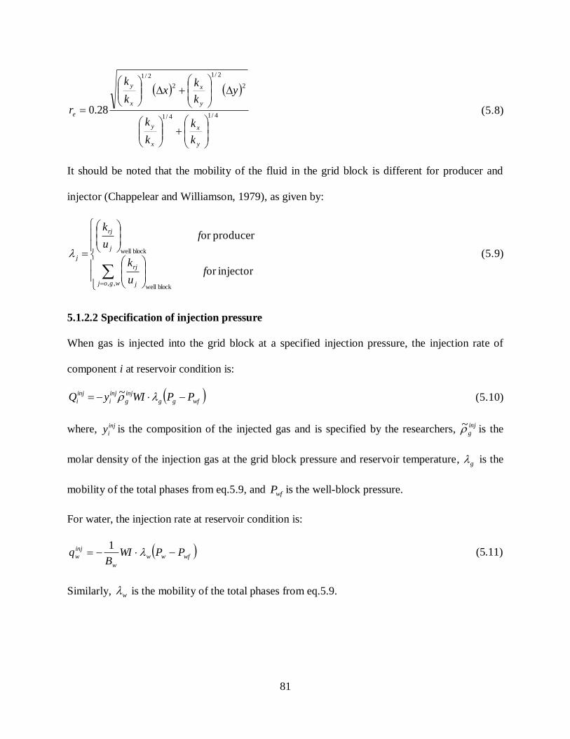
81

4/14/1

2

2/1

2

2/1

28.0

y

x

x

y

y

x

x

y

e

k

k

k

k

yk

kx

k

k

r (5.8)

It should be noted that the mobility of the fluid in the grid block is different for producer and

injector (Chappelear and Williamson, 1979), as given by:

injector or

producer or

,,block well

block well

fu

k

fu

k

wgoj j

rj

j

rj

j (5.9)

5.1.2.2 Specification of injection pressure

When gas is injected into the grid block at a specified injection pressure, the injection rate of

component i at reservoir condition is:

wfgg

inj

g

inj

i

inj

i PPWIyQ ~ (5.10)

where, inj

iy is the composition of the injected gas and is specified by the researchers, inj

g~ is the

molar density of the injection gas at the grid block pressure and reservoir temperature, g is the

mobility of the total phases from eq.5.9, and wfP is the well-block pressure.

For water, the injection rate at reservoir condition is:

wfww

w

inj

w PPWIB

q 1

(5.11)

Similarly, w is the mobility of the total phases from eq.5.9.

82

5.1.2.2 Specification of production rate

When the production rate of a phase is specified, the molar production of component i at surface

condition is:

pN

j

jjiji qQ1

~ (5.12)

The water production rate at surface condition is:

w

wscw

B

qq ,

(5.13)

5.1.2.4 Specification of injection rate

When the gas injection rate at surface condition is specified, the injection rate of component i at

reservoir condition is calculated as:

RT

Pq

yQ

sc

scinj

scg

inj

iinj

i ,615.5

(5.14)

5.1.3 Numerical Solution

The finite difference approach is applied to solve the mole balance equations for multi-components

mass balance (eq.5.1) and water volume balance (eq. 5.2). Transmissibility terms are used here to

measure how much fluid flows into or out of the grid block. A Jacobian matrix is established with

entries of partial derivatives of residuals with respect to the principal unknowns and linear solver

to solve the Jacobian matrix is used.

5.1.3.1 Finite difference approximation

The backward time central space (BTCS) finite difference method is used. For component i, the

mole balance equation can be expressed as:

83

pp

p

p

N

j

n

zyxjij

n

zyxjijb

N

j

ij

N

j

n

zyx

n

zyxzyx

rjzz

j

jj

c

in

zyx

n

zyxzyx

rjzz

j

jj

c

ij

n

zyx

n

zyxzyx

rjyy

j

jj

c

in

zyx

n

zyxzyx

rjyy

j

jj

c

ij

n

zyx

n

zyxzyx

rjxx

j

jj

c

in

zyx

n

zyxzyx

rjxx

j

jj

c

ij

N

j

n

zyxj

n

zyxjzyx

rjzz

j

j

ij

n

zyxj

n

zyxjzyx

rjzz

j

j

ij

n

zyxj

n

zyxjzyx

rjyy

j

j

ij

n

zyxj

n

zyxjzyx

rjyy

j

j

ij

n

zyxj

n

zyxjzyx

rjxx

j

j

ij

n

zyxj

n

zyxj

n

zyx

rjxx

j

j

ij

SSV

M

GGz

kkA

ug

gGG

z

kkA

ug

g

GGy

kkA

ug

gGG

y

kkA

ug

g

GGx

kkA

ug

gGG

x

kkA

ug

g

PPz

kkA

uPP

z

kkA

u

PPy

kkA

uPP

y

kkA

u

PPx

kkA

uPP

x

kkA

u

1

,,

1

,,

1

1

1

1,,

1

,,

2

1,,

1

,,

1

1,,

2

1,,

1

,1,

1

,,,

2

1,

1

,,

1

,1,,

2

1,

1

,,1

1

,,,,

2

1

1

,,

1

,,1,,

2

1

1

1

1,,

1

,,

2

1,,

1

,,

1

1,,

2

1,,

1

,1,

1

,,,

2

1,

1

,,

1

,1,,

2

1,

1

,,1

1

,,,,

2

1

1

,,

1

,,1

1

,,2

1

~~

615.5

~

144

~

144

~

144

~

144

~

144

~

144

~~

~~

~~

(5.15)

The convective transmissibility is extracted from eq. 5.15 and is used to describe the amount of

fluid exchange from the grid block that is driven by convective flow. The expressions of

transmissibility for x and y directions are:

1

,,2

1,,

2

1

1

,,2

1

1

,,2

1,

~

n

zyxrjij

zyx

xxn

zyxj

jn

zyxxij k

x

kA

uT

(5.16)

1

,2

1,,

2

1,

1

,2

1,

1

,2

1,

,

~

n

zyxrjij

zyx

yyn

zyxj

jn

zyxyij k

y

kA

uT

(5.17)

1

2

1,,

2

1,,

1

2

1,,

1

2

1,,

,

~

n

zyxrjij

zyx

yyn

zyxj

jn

zyxzij k

y

kA

uT

(5.18)

1

,,2

1,

1

,,2

1

1

,,2

1,144

1

n

zyxxij

n

zyxj

c

n

zyxxijG T

g

gT

84

By using the finite difference approximation, the water volume balance equation can be express

as:

n

zyx

w

on

zyx

w

obwell

w

n

zyx

n

zyxzyx

rwzz

ww

w

c

n

zyx

n

zyxzyx

rwzz

ww

w

c

n

zyx

n

zyxzyx

rwyy

ww

w

c

n

zyx

n

zyxzyx

rwyy

ww

w

c

n

zyx

n

zyxzyx

rwxx

ww

w

c

n

zyx

n

zyxzyx

rwxx

ww

w

c

n

zyxw

n

zyxwzyx

rwzz

ww

n

zyxw

n

zyxwzyx

rwzz

ww

n

zyxw

n

zyxwzyx

rwyy

ww

n

zyxw

n

zyxwzyx

rwyy

ww

n

zyxw

n

zyxwzyx

rwxx

ww

n

zyxw

n

zyxw

n

zyx

rwxx

ww

B

S

B

SVq

GGz

kkA

Bug

gGG

z

kkA

Bug

g

GGy

kkA

Bug

gGG

y

kkA

Bug

g

GGx

kkA

Bug

gGG

x

kkA

Bug

g

PPz

kkA

BuPP

z

kkA

Bu

PPy

kkA

BuPP

y

kkA

Bu

PPx

kkA

BuPP

x

kkA

Bu

,,

1

,,

1

1,,

1

,,

2

1,,

1

,,

1

1,,

2

1,,

1

,1,

1

,,,

2

1,

1

,,

1

,1,,

2

1,

1

,,1

1

,,,,

2

1

1

,,

1

,,1,,

2

1

1

1,,

1

,,

2

1,,

1

,,

1

1,,

2

1,,

1

,1,

1

,,,

2

1,

1

,,

1

,1,,

2

1,

1

,,1

1

,,,,

2

1

1

,,

1

,,1

1

,,2

1

615.5

144

1

144

1

144

1

144

1

144

1

144

1

11

11

11

(5.19)

5.1.3.2 Jacobian matrix

Flow equations for matrix domain is solved based on fully implicit formulation using the Newton-

Raphson method. Eq. 5.20 represents system of equations solved at every iteration level in matrix

domain. R represents residual. The principle unknowns are oil pressure (Po), water saturation (Sw),

and overall compositions of water and Nc‒1 other non-aqueous components. The total number of

unknowns are Nc+1.

RXJ (5.20)

The Jacobian is calculated as:

85

121

121

1

3

2

3

1

333

1

2

2

2

1

222

1

1

2

1

1

111

...

...

..................

...

...

...

Nc

www

w

w

o

w

Nc

NcNcNc

w

Nc

o

Nc

Ncwo

Ncwo

Ncwo

dZ

dR

dZ

dR

dZ

dR

dS

dR

dP

dR

dZ

dR

dZ

dR

dZ

dR

dS

dR

dP

dR

dZ

dR

dZ

dR

dZ

dR

dS

dR

dP

dR

dZ

dR

dZ

dR

dZ

dR

dS

dR

dP

dR

dZ

dR

dZ

dR

dZ

dR

dS

dR

dP

dR

J

(5.21)

The unknown vector of X is arranged as:

121 ,...,,, Ncwo ZZZSPX (5.22)

R is the vector of residuals of conservation equations and is expressed as:

wNc RRRRRR ,...,, 1321 (5.23)

The elements in the Jacobian matrix and residual vector is calculated by using numerical

differentiation.

5.1.3.3 Linear solver

In this study, the generalized minimal residual method (GMRES) as an iterative method is used to

get the numerical solution. GMRES is designed for nonsymmetrical linear systems. The solver

was developed by Lili Ju and John Burkardt, University of South Carolina. The incomplete LU

decomposition approach is implemented as a preprocessor.

5.1.4. Relative permeability

Stone’s Model II (Stone, 1973) is used as a predictor to estimate the relative permeabilities.

rgrwrg

rocw

rog

rw

rocw

row

rocw

ro kkkk

kk

k

k

k

k

(5.24)

86

wrw Sfk , grg Sfk , and woro SSfk , (5.25)

5.2 Phase Behavior Model

Predicting the behaviors of hydrocarbon in gas and liquid phase at reservoir condition is

required when modeling the compositional behavior.

5.2.1 Equation of state

The Peng-Robison Equation of State (PR-EOS) (Peng and Robinson, 1976)) is chosen as the

phase behavior model and is used in this in-house simulator. The purpose is to get the Z

(compressibility factor) of vapor or liquid phase by solving the cubic equation as follows.

0)]1([)]1()([]1)1[( 2

2121

2

21

2

21

3 BBmmABZBBmmBmmAZBmmZ

(5.26)

The detailed formulations about PR-EOS can be found in Appendix A.

5.2.2 Vapor-Liquid Equilibrium

The equilibrium ratios (Ki) is defined as the ratio of the mole fraction of component i in the

gas phase (yi) to the mole fraction of component i in the liquid phase (xi), given as:

i

ii

x

yK (5.27)

For a two-phase (oil and gas phases) system at equilibrium state, Rachford and Rice (1952)

suggested the following equation:

0)1(1

)1()(

1

cn

i ing

iing

Kf

Kcfg (5.28)

The above Rachford-Rice Objective Function is used to solve the gas mole fraction in the

mixture ( ngf ), given that the K-values are known. Generally, Newton Raphson iterative approach

87

is used to solve the gas fraction (ngf ). Newton Raphson method is fast but may lead to an

unphysically acceptable range. In that case, the Bisection method is used. The detailed procedure

of two methods are discussed in Appendix B.

Here, we use the Wilson’s correlation to provide an approximate value for initial Ki.

)

11)(1(37.5

1

ri

i

ri

iT

EXPP

K (5.29)

Since Wilson’s correlation only gives an approximate prediction for equilibrium ratios, more

reliable K-values are required by applying the thermodynamic equilibrium. At thermodynamic

equilibrium state, the chemical potentials for all the phases should be the same. In other words, the

fugacities of component i in oil and gas phases are equal, i.e.:

gili ff (5.30)

where, lif is the fugacity of component i in the liquid phase, and lif is the fugacity of component

i in the gas phase. To calculate the fugacity, the fugacity coefficient is introduced, which is defined

as the ratio of the fugacity of a component to its partial pressure. The fugacity coefficient of

component i for gas and liquid phases are given as:

Py

f

i

gi

gi (5.31)

Px

f

i

lili (5.32)

For a generalized cubic equation of state, the fugacity coefficient of component i for one phase is

calculated as:

88

)1(ln

2

)()ln(ln

1

21

21

ZB

B

BmZ

BmZ

B

B

A

cA

Bmm

ABZ ii

n

j

jij

i

c

(5.33)

where, Z-factor is the for the liquid and gas phases, and jc is the corresponding phase composition

To achieve the thermodynamic equilibrium, the successive substitution method (SSM) is

applied. The K-value is related to the fugacity coefficient of li and gi .

gi

li

i

i

gi

lii

f

f

x

yK

(5.34)

For SSM, we updated the K-values as follows:

n

gi

li

n

i

in

if

f

x

yK

1 (5.35)

n

gi

lin

i

n

if

fKK

1 (5.36)

The convergence is achieved when:

10

2

101

n

i gi

li

f

f (5.37)

5.2.3 Phase properties

Once the vapor fraction ( ngf ) and K-values are determined from SSM, the phase compositions

are calculated by using the following equations:

)1(1

ing

ii

Kf

cx (5.38)

)1(1

ing

iii

Kf

cKy (5.39)

89

We can calculate more important phase properties by applying the obtained phase compositions.

The calculations of molecular weight, density, viscosity, saturation of oil and gas phases are shown

in Appendix C.

5.3Validation results

In this section, we validate the developed in-house compositional simulator through cross-

checking the results CMG (GEM). The hydrocarbon components that were used include CH4, NC4,

NC7, and NC10, and their properties are tabulated in Table 5.1. The binary interaction parameters

are given in Table 5.2.

Table 5.1 The properties of hydrocarbon components for validation tests.

Mole

fraction Pc (psia) Tc (R)

Acentric

factor

Mw

(lb/lbmol)

Critical

volume

(ft3/lbmol) Parachor

CH4 0.2 667.1961 343.08 0.008 16.043 1.586 77

NC4 0.3 551.0981 765.36 0.193 58.124 4.085 189.9

NC7 0.3 396.791 972.36 0.351 100.205 6.921 312.5

NC10 0.2 305.6757 1111.68 0.49 142.286 9.66 433.5

Table 5.2 The binary interaction parameters of hydrocarbon components.

CH4 NC4 NC7 NC10

CH4 0 0 0 0

NC4 0 0 0 0

NC7 0 0 0 0

NC10 0 0 0 0

The relative permeability curves for validation tests are plotted in Figure 5.1.

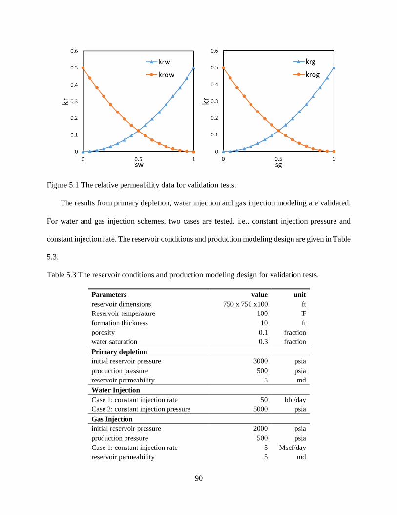
90

Figure 5.1 The relative permeability data for validation tests.

The results from primary depletion, water injection and gas injection modeling are validated.

For water and gas injection schemes, two cases are tested, i.e., constant injection pressure and

constant injection rate. The reservoir conditions and production modeling design are given in Table

5.3.

Table 5.3 The reservoir conditions and production modeling design for validation tests.

Parameters value unit

reservoir dimensions 750 x 750 x100 ft

Reservoir temperature 100 ̊F

formation thickness 10 ft

porosity 0.1 fraction

water saturation 0.3 fraction

Primary depletion

initial reservoir pressure 3000 psia

production pressure 500 psia

reservoir permeability 5 md

Water Injection

Case 1: constant injection rate 50 bbl/day

Case 2: constant injection pressure 5000 psia

Gas Injection

initial reservoir pressure 2000 psia

production pressure 500 psia

Case 1: constant injection rate 5 Mscf/day

reservoir permeability 5 md

91

Case 2: constant injection pressure 2000 psia

reservoir permeability 0.5 md

For the primary depletion scheme, the reservoir is initially in single‒oil phase and

experiences phase change during the production process. The producer well block pressure, oil

production rate, gas production rate, and water production rate versus time are plotted in Figure

5.2.

Figure 5.2 Validation of primary depletion. For the producer well block: (a) well block pressure;

(b) oil production rate; and (c) gas production rate; and (d) water production rate.

For water injection scheme, the constant injection rate (50 bbl/day) and constant injection

pressure (5000 psia) are separately validated. The results for producer and injector are plotted in

92

Figure –Figure. We also plotted the water saturation distributions at different times in Figure and

Figure. From the plot, the water breaks through at 920 days and 910 days respectively.

Figure 5.3 Validation of water injection at constant injection rate of 50 bbl/day. For the producer

well block: (a) well block pressure; (b)water production rate; (c) oil production rate; and (d) gas

production rate.

93

Figure 5.4 Validation of water injection at constant injection rate of 50 bbl/day. For injector well

block: (a) well block pressure; (b) water injection rate

1 day 100 days 200 days 500 days 1000 days

Figure 5.5 Water saturation distributions at different times at constant injection rate of 50 bbl/day.

Sw

94

Figure 5.6 Validation of water injection at constant injection pressure of 5000 pisa. For the

producer well block: (a) well block pressure; (b)water production rate; (c) oil production rate; and

(d) gas production rate.

Figure 5.7 Validation of water injection at constant injection pressure of 5000 psia. For injector

well block: (a) well block pressure and (b) water injection rate.

1 day 100 days 200 days 500 days 1000 days

Figure 5.8 Water saturation distributions at different times at constant injection pressure of 5000

psia.

For gas injection scheme, the constant injection rate (5 Mscf/day) and constant injection

pressure (2000 psia) are separately validated. The results for producer and injector are plotted in

Figure5.9 –Figure 5.10. We also plotted the gas saturation distributions at different times for

constant gas injection rate and pressure distributions at different times for constant injection

Sw

95

pressure in Figure and Figure. From the plot, the gas breaks through at 2430 days for the scheme

of constant gas injection rate.

Figure 5.9 Validation of gas injection at constant injection rate of 5 Mscf/day. For the producer

well block: (a) well block pressure; (b)water production rate; (c) oil production rate; and (d) gas

production rate.

96

Figure 5.10 Validation of gas injection at constant injection rate of 5 Mscf/day. For injector well

block: (a) well block pressure; (b) gas injection rate

1 day 100 days 300 days 500 days 1000 days

1500 days 2000 days 2430 days

Figure 5.11 Gas saturation distributions at different times at constant gas injection rate of 5

Mscf/day.

Sg

97

Figure 5.12 Validation of gas injection at constant injection pressure of 2000 psia. For the producer

well block: (a) well block pressure; (b)water production rate; (c) oil production rate; and (d) gas

production rate.

Figure 5.13 Validation of gas injection at constant injection pressure of 2000 psia. For injector

well block: (a) well block pressure; (b) gas injection rate

1 day 100 days 500 days 800 days 1000 days

Figure 5.14 Pressure distributions at different times at constant gas injection pressure of 2000 psia.

Overall, the validation results for primary depletion, water injection, and gas injection show a

good match with commercial software.

P (psia)

98

5.4 Nano-confinement effects

In this section, the nano-confinement effects (critical property shift and capillary pressure effect)

on shale oil and shale gas production would be examined by using the developed fully

compositional simulator. The matrix permeability in the stimulated reservoir volume (SRV) is

increased caused by the fracking. The corresponding pore size should also be increased. However,

in previous studies, the enlargement of pore size in SRV is not considered while examine the nano-

confinement effects. In this study, the pore size variation in SRV will be considered by correlating

the pore size with permeability.

5.4.1 Critical property shift

In nanoscale porous media, a significant reduction of critical temperatures of several substances

have been observed in the experimental work of Morishige et al. (1997). Zarragoicoechea and Kuz

(2004) developed models to account for the shift of both critical pressure and critical temperature.

The effect of critical property shift on diffusion coefficient has been discussed in Section 4.4.1.

The equations of critical property shifts are given in Section 4.4.1, as shown in Eq.4.19-4.21. In

this section, the critical property shift as a function of pore radius will be reflected in the flash

calculation.

5.4.2 Oil–gas capillary pressure

The oil-gas capillary pressure effect on estimation of diffusion coefficient has been discussed

in Section 4.4.2. Meanwhile, the oil-gas capillary pressure effect on production has also been

investigated in Section 3.4 by using a reduced compositionally black-oil type model. By using

black oil model, the fluid properties with and without considering capillary pressure need to be

calculated prior to performing the reservoir simulation. The advantage is that we only need to run

the flash calculation once. The disadvantage is that for a heterogeneous reservoir with varied pore

99

size, the fluid properties as a function of all possible pore sizes are required to calculated prior to

simulation. Therefore, much more preliminary work is required compared to single pore size

scheme. In this section, a fully compositional model is used to examine the oil-gas capillary

pressure. The fluid properties as a function of pore size and oil-gas interfacial tension is updated

at each iteration. The oil-gas capillary pressure in both flash calculation and in fluid flow are

incorporated. The pore size is correlated to the permeability. The pore throat aperture as a function

of permeability that developed by Gao and Hu (2013) is used:

214.0log225.2log prk (5.40)

The wetting phase is assumed to be the wetting phase. Oil pressure is taken as the reference

phase pressure. The expressions of gas pressure and interfacial tension as a function of phase molar

density and phase compositions have been given in Eq. 4.22 and 4.23.

At thermodynamic equilibrium state, the fugacities of component i in the vapor and liquid

phases are identical, despite the fact that the phase pressures are not, i.e.,

NcggiNcoli yyyPTfxxxPTf ,...,,,,...,,, 2121 (5.41)

The fugacity coefficients of component i for liquid and vapor phases are defined as:

oi

lili

Px

f (5.42)

gi

gi

giPy

f (5.43)

The equilibrium constant K-value, defined as the 𝐾𝑖 = 𝑦𝑖/𝑥𝑖, in the successive substitution method

(SSM) is rewritten as:

n

o

g

n

gi

lin

i

n

o

g

n

gi

li

n

i

in

iP

P

f

fK

P

P

f

f

x

yK

1 (5.44)

100

An thermodynamic phase equilibrium state is reached until

14

2

101

n

i gi

li

f

f (5.45)

5.4.3 Simulation results

In this study, the Bakken crude oil (Nojabaei et al., 2013) and Marcellus shale gas (Bullin et

al., 2008) are used. For Marcellus shale gas, the reservoir fluid is single gas phase at the reservoir

temperature of 140 ̊F, as shown in Figure 4.6. The gas-oil capillary pressure is zero and only the

critical property shifts nano-confinement effect is taken into consideration.

5.4.3.1 Confinement effects on shale oil

For Bakken oil, the original eight components are lumped into five pseudo-components. The

reservoir temperature is 240 °F. The molar fraction of the five components at reservoir conditions

and the critical properties used in Peng-Robinson EOS are given in Table 5.4. The binary-

interaction parameters (BIP) of the five pseudo-components are recalculated use weight-based

grouping approach. Bubble point pressure is 2768 psia. The results are tabulated in Table 5.5.

Table 5.4 Compositions and parameters of Bakken oil.

Component Mole

fraction

Critical

Pressure (psia)

Critical

temperature (oR)

Acentric

factor

Mole

weight Parachor

C1 0.36736 655.02 335.34 0.01020 16.54 74.8

C2-C3 0.24219 681.05 594.68 0.12176 35.70 124.7

C4-C6 0.12157 501.58 820.48 0.23103 68.75 221.5

C7-C12 0.15854 363.34 1053.25 0.42910 120.56 350.2

C13-C80 0.11034 229.64 1504.10 0.81953 295.51 800.4

Table 5.5 Binary interaction coefficients of Bakken oil.

C1 C2-C3 C4-C6 C7-C12 C13-C80

C1 0 0.0044 0.0036 0.0033 0.0033

C2-C3 0.0044 0 0.0019 0.0016 0.0016

101

C4-C6 0.0036 0.0019 0 0 0

C7-C12 0.0033 0.0016 0 0 0

C13-C80 0.0033 0.0016 0 0 0

A reservoir domain with 15 by 15 grid blocks is used. The producer is located at the center of

the reservoir domain. The initial reservoir pressure is 2500 psia and the production pressure is 500

psia. The initial water saturation is 0.25. The total production time is 1000 days. We increase the

matrix permeability near the production well to account for the stimulated reservoir volume (SRV)

in the reservoir that is caused by hydraulic fractures. The reservoir permeability map is shown in

Figure 5.15. Here, the matrix permeability is 0.05 md. The Middle Bakken formation is considered

as the prototype, and the reservoir is not ultra-tight, but only tight. The mass transfer is completely

convection-dominated as the permeability is relatively large.

Figure 5.15 Reservoir permeability map for tight oil-rich reservoir.

Two schemes of reservoir pore size are implemented, as plotted in Figure 5.16 (a) and (b). In

Figure 5.16 (a), a constant pore size is used for the entire reservoir, and this is also how we treated

the confinement effects in a reservoir domain by using the black oil type model. The fixed pore

throat size of 19 nm is from a Bakken sample rock (Nojabaei et al., 2013). In Figure 5.16 (b), the

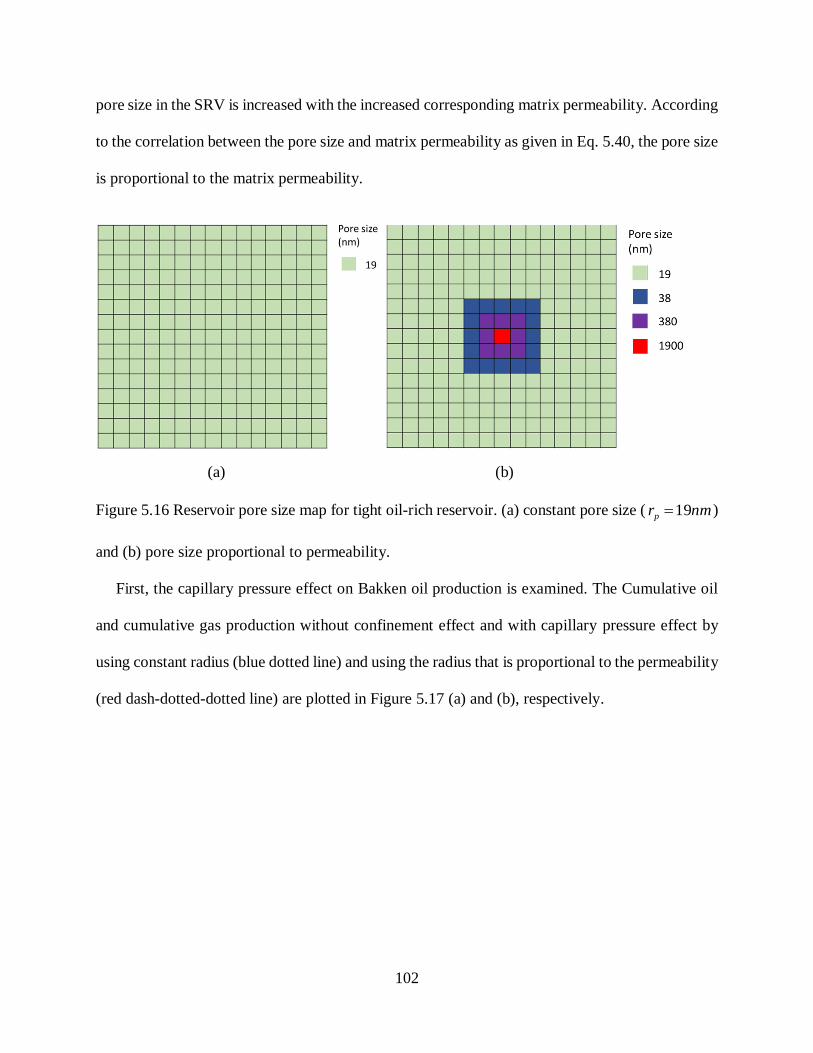
102

pore size in the SRV is increased with the increased corresponding matrix permeability. According

to the correlation between the pore size and matrix permeability as given in Eq. 5.40, the pore size

is proportional to the matrix permeability.

(a) (b)

Figure 5.16 Reservoir pore size map for tight oil-rich reservoir. (a) constant pore size ( nmrp 19 )

and (b) pore size proportional to permeability.

First, the capillary pressure effect on Bakken oil production is examined. The Cumulative oil

and cumulative gas production without confinement effect and with capillary pressure effect by

using constant radius (blue dotted line) and using the radius that is proportional to the permeability

(red dash-dotted-dotted line) are plotted in Figure 5.17 (a) and (b), respectively.

103

Figure 5.17 (a) Cumulative oil and (b) cumulative gas production without confinement effect and

with capillary pressure effect by using constant radius ( nmrp 19 ) and using the radius that is

proportional to the permeability.

As shown in Figure 5.17, inclusion of capillary pressure effect significantly increases the oil

production, but suppresses the gas production no matter which pore size scheme is used. This result

is consistent with the finding from the literature (Du et al., 2020). For the scheme that uses fixed

pore size, the effect of capillary pressure on increasing the oil production or decreasing the gas

production is more obvious. As is expected, for the scheme of the pore throat radius that is

104

proportional to the permeability, the effect of capillary pressure on production is much reduced,

especially in the early period where oil or gas is mainly produced from the high permeable SRV.

1 day 100 days 200 days 500 days 1000 days

(a)

1 day 100 days 200 days 500 days 1000 days

(b)

Figure 5.18 Oil-gas capillary pressure distributions at different production times by using (a)

constant pore size ( nmrp 19 ) and (b) pore size proportional to permeability.

We visualized the distribution of oil-gas capillary pressure in the reservoir domain at different

production times for both pore size schemes, as shown in Figure 5.18. For fixed pore size, i.e.,

Figure 5.18 (a), the oil-gas capillary pressure in the SRV could reach up to 400 psi. In Figure 5.18

(b), the oil-gas capillary pressure is very small owing to the very large pore size in the SRV.

1 day 100 days 200 days 500 days 1000 days

Pc (psia)

105

(a)

1 day 100 days 200 days 500 days 1000 days

(b)

Figure 5.19 Oil-gas interfacial tension at different grid blocks at different production times by

using (a) constant pore size ( nmrp 19 ) and (b) pore size proportional to permeability.

We also visualized the oil-gas interfacial tension for both pore size schemes, as plotted in

Figure 5.19. For fixed pore size, the oil-gas interfacial tension becomes larger as the pressure

decreases with time. This explains the increasing oil-gas capillary pressure for fixed pore size

scheme. For the pore size that is proportional to the permeability, the oil-gas interfacial tension is

also increasing as pressure decreases, but the oil-gas capillary pressure in the SRV is still very

small since it still cannot compensate loss caused by the very large pore size.

IFT

(dyne/cm)

106

Figure 5.20 (a) Cumulative oil and (b) cumulative gas production without confinement effect and

with critical property shift effect by using constant pore size ( nmrp 19 ) and using the pore size

that is proportional to the permeability.

In this section, we also examine the effect of critical property shift on Bakken oil production.

In Figure 5.20 (a) and (b), the cumulative oil production and gas production without confinement

effect and with critical property shift effect by using two pore sizes schemes are plotted,

respectively. Oil production is significantly increased with considering critical property shift.

Similarly, the rise of oil production using varied pore size lags behind the scheme using fixed pore

size. This is because the effect of critical property shift is negligible in early production period

when the fluid is produced from the SRV with large pore size. In figure 5.20 (b), including critical

property shift decreases the gas production slightly for the constant pore size scheme. The effect

of critical property shifts on gas production is very small and almost negligible for the scheme of

using pore size proportional to permeability.

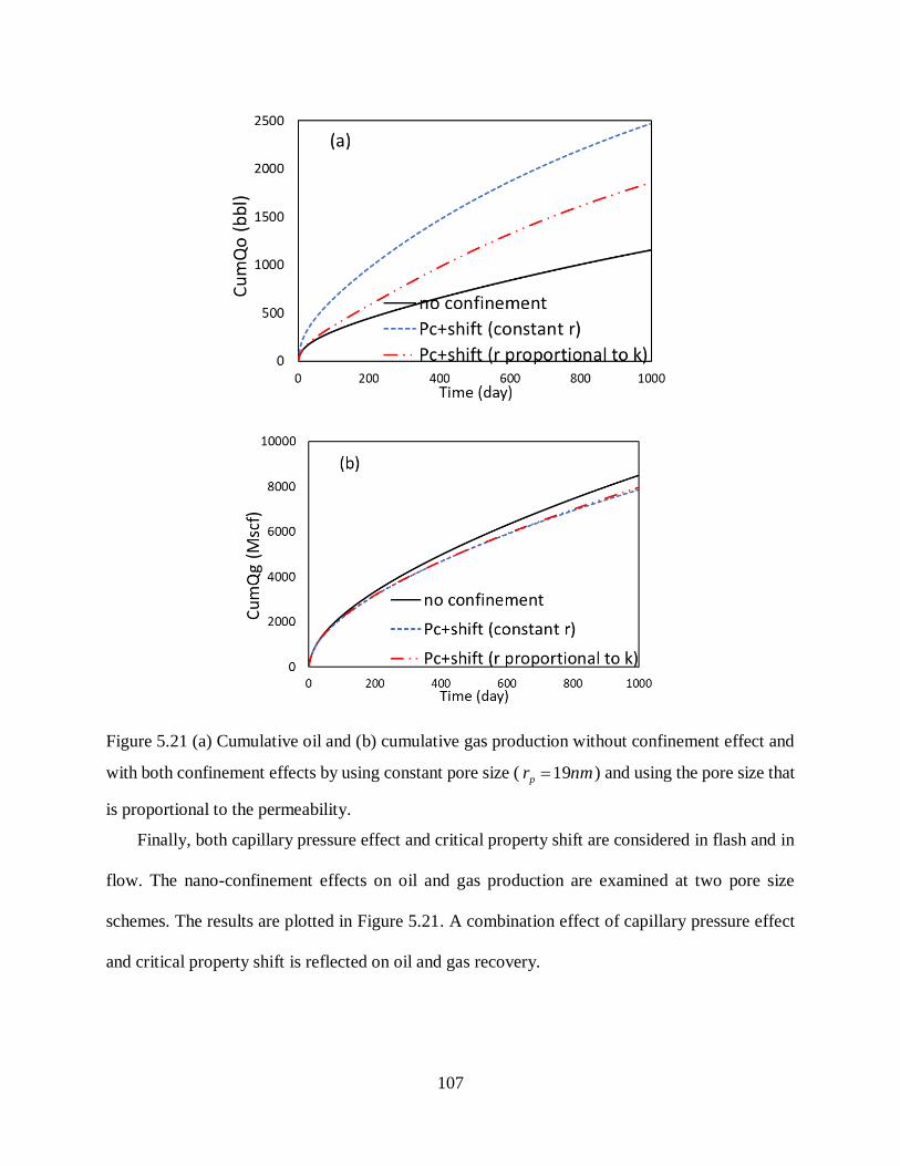
107

Figure 5.21 (a) Cumulative oil and (b) cumulative gas production without confinement effect and

with both confinement effects by using constant pore size ( nmrp 19 ) and using the pore size that

is proportional to the permeability.

Finally, both capillary pressure effect and critical property shift are considered in flash and in

flow. The nano-confinement effects on oil and gas production are examined at two pore size

schemes. The results are plotted in Figure 5.21. A combination effect of capillary pressure effect

and critical property shift is reflected on oil and gas recovery.

108

Table 5.6 Cumulative oil and gas production without confinement effects and with confinement

effects by using constant pore size ( nmrp 19 ) and using the pore size that is proportional to the

permeability.

Confinement effects Qo

(bbl)

increased

Qo (%)

Qg

(Mscf)

increased

Qg (%)

constant

radius

no confinement 1155.05 – 8482.66 –

shift 1517.44 31.37 8532.95 0.59

Pc 2003.31 73.44 7549.82 -11.00

shift+Pc 2469.60 113.81 7836.82 -7.61

radius

proportional

to k

no confinement 1155.05 – 8482.66 –

shift 1426.64 23.51 8379.06 -1.22

Pc 1474.36 27.64 7922.28 -6.61

shift+Pc 1850.46 60.21 7955.46 -6.22

The increased or decreased percentage of oil and gas production after considering confinement

effects are calculated and tabulated in Table 5.6. In summary, both critical property shift and

capillary pressure effect increases the oil production. For the case of considering capillary pressure,

when the pore size is proportion to the permeability in the SRV, the increased oil production is

half of the increased oil production while using constant pore size. However, for the case of

including critical property shift, the increased oil production differs not that much for both pore

size schemes.

5.4.3.1 Confinement effects on shale gas production

For Marcellus shale gas, the compositions have been given in Table 4.1. The binary interaction

coefficients are given in Table 5.7. The reservoir permeability map is shown in Figure 5.22 and

the matrix permeability is 0.00005 md. Again, the matrix permeability near the production well is

increased to account for the stimulated reservoir volume (SRV) in the reservoir that is caused by

hydraulic fractures.

Table 5.7 Binary interaction coefficients of Marcellus shale gas

109

CO2 C1 C2 C3 N2

CO2 0 0.1 0.13 0.135 -0.02

C1 0.1 0 0 0 0.036

C2 0.13 0 0 0 0.05

C3 0.135 0 0 0 0.08

N2 -0.02 0.036 0.05 0.08 0

Figure 5.22 Reservoir permeability map with matrix permeability as 0.00005 md.

For Marcellus shale gas, the reservoir fluid is in single gas phase. The gas-oil capillary pressure

is zero and only the critical property shifts is taken into consideration. In Figure 5.23, the

cumulative gas production with critical property shift is examined under two pore size schemes.

Similar to the gas production of Bakken oil, including critical property shift reduces the gas

production very slightly.

110

Figure 5.23 Cumulative gas production without confinement effect and with critical property shift

effect by using constant pore size ( nmrp 19 ) and using the pore size that is proportional to the

permeability.

5.5 Molecular diffusion effect

A recent molecular simulation study indicated that, at pore size of 10 nm or even 5 nm,

molecular diffusion still occurs in those nano-pores (Wang et al., 2016). In such ultra-tight low

permeability reservoirs, molecular diffusion is comparable to the convection viscous flow and

mass transfer is expected to be diffusion-dominated (Cronin et al., 2019). In many gas injection

studies of shale reservoirs, different attempts have been made to examine the role of molecular

diffusion in gas injection process for EOR/EGR. A review study revealed that the molecular

diffusion effect on improving shale oil and gas recovery is highly sensitive to the employed

diffusion coefficient (Du and Nojabaei, 2019). Owing to the lack of reference data, most studies

assumed a diffusivity based on the literature. In this section, we will examine the role of molecular

diffusion in huff-n-puff Bakken oil production and Marcellus shale gas production. The molecular

diffusion coefficient is calculated by using the Sigmund correlation (Sigmund et al., 1976a;1976b).

The governing equation of Eq. 5.1 is modified by adding the diffusive term, as shown below:

111

ppp p N

j

jijj

N

j

ij

N

j

N

j

ijj

j

rj

jij St

QJkk

111 1

~~

(5.46)

The Fick’s classical model is used and the diffusion flux is expressed as:

jijijjij DSJ ~ (5.47)

The backward time central space (BTCS) finite difference method is used. For component i,

the mole balance equation with considering molecular diffusion can be expanded as:

pp

p

p

p

N

j

n

zyxjij

n

zyxjijb

N

j

ij

N

j

n

zyx

n

zyxzyx

rjzz

j

jj

c

in

zyx

n

zyxzyx

rjzz

j

jj

c

ij

n

zyx

n

zyxzyx

rjyy

j

jj

c

in

zyx

n

zyxzyx

rjyy

j

jj

c

ij

n

zyx

n

zyxzyx

rjxx

j

jj

c

in

zyx

n

zyxzyx

rjxx

j

jj

c

ij

N

j

n

zyxjij

n

zyxjijzyx

zjijn

zyxjij

n

zyxjij

n

zyx

zjij

n

zyxjij

n

zyxjijzyx

yjijn

zyxjij

n

zyxjij

n

zyx

yjij

n

zyxjij

n

zyxjijzyx

xjijn

zyxjij

n

zyxjij

n

zyx

xjij

N

j

n

zyxj

n

zyxjzyx

rjzz

j

j

ij

n

zyxj

n

zyxjzyx

rjzz

j

j

ij

n

zyxj

n

zyxjzyx

rjyy

j

j

ij

n

zyxj

n

zyxjzyx

rjyy

j

j

ij

n

zyxj

n

zyxjzyx

rjxx

j

j

ij

n

zyxj

n

zyxj

n

zyx

rjxx

j

j

ij

SSV

M

GGz

kkA

ug

gGG

z

kkA

ug

g

GGy

kkA

ug

gGG

y

kkA

ug

g

GGx

kkA

ug

gGG

x

kkA

ug

g

z

ASD

z

ASD

y

ASD

y

ASD

x

ASD

x

ASD

PPz

kkA

uPP

z

kkA

u

PPy

kkA

uPP

y

kkA

u

PPx

kkA

uPP

x

kkA

u

1

,,

1

,,

1

1

1

1,,

1

,,

2

1,,

1

,,

1

1,,

2

1,,

1

,1,

1

,,,

2

1,

1

,,

1

,1,,

2

1,

1

,,1

1

,,,,

2

1

1

,,

1

,,1,,

2

1

1

1

1,,

1

,,

2

1,,

1

,,

1

1,,

1

2

1,,

1

,1,

1

,,,

2

1,

1

,,

1

,1,

1

,2

1,

1

,,1

1

,,,,

2

1

1

,,

1

,,1

1

,,2

1

1

1

1,,

1

,,

2

1,,

1

,,

1

1,,

2

1,,

1

,1,

1

,,,

2

1,

1

,,

1

,1,,

2

1,

1

,,1

1

,,,,

2

1

1

,,

1

,,1

1

,,2

1

~~

615.5

~

144

~

144

~

144

~

144

~

144

~

144

~~

615.5

~~

615.5

~~

615.5

~~

615.5

~~

615.5

~~

615.5

~~

~~

~~

(5.48)

112

The diffusive transmissibility that extracted from the above equation is used to describe the

amount of fluid exchange from the grid block driven by molecular diffusion. The expressions of

diffusive transmissibility for x, y, and z directions are:

1

,,2

1

1

,,2

1

1

,,2

1,615.5

n

zyx

xn

zyxj

n

zyxij

ij

xijx

AS

DTD (5.49)

1

,2

1,

1

,2

1,

1

,2

1,

,615.5

n

zyx

yn

zyxj

n

zyxij

ij

yijy

AS

DTD (5.50)

1

2

1,,

1

2

1,,

1

2

1,,

,615.5

n

zyx

zn

zyxj

n

zyxij

ij

zijz

AS

DTD (5.51)

The huff-n-puff gas injection scheme is used to examine the diffusion effect by injecting CO2

into Bakken oil and into Marcellus shale gas.

5.5.1 Molecular diffusion in Bakken oil

The binary interaction coefficient of CO2 with Bakken oil are tabulated in Table 5.8. The

reservoir is a square domain and the fracture caused stimulated reservoir volume is in the center.

The reservoir permeability map is shown in Figure 5.24. The pore size that is correlated to

permeability is used in this section.

Table 5.8 Binary interaction coefficient of Bakken oil with CO2.

CO2 C1 C2-C3 C4-C6 C7-C12 C13-C80

CO2 0 0.1 0.13 0.125 0.1 0.08

C1 0.1 0 0.0044 0.0036 0.0033 0.0033

C2-C3 0.13 0.0044 0 0.0019 0.0016 0.0016

C4-C6 0.125 0.0036 0.0019 0 0 0

C7-C12 0.1 0.0033 0.0016 0 0 0

C13-C80 0.08 0.0033 0.0016 0 0 0

113

Figure 5.24 Reservoir permeability map with matrix permeability as 0.001 md.

The single well is located at the center. After primary depletion for 150 days, CO2 is injected

into the reservoir at injection rate of 5 Mscf/day for 30 days, followed by 15 days of shut-in period.

The cumulative oil and cumulative gas production without molecular diffusion (black line) and

with molecular diffusion (blue dotted line) are plotted in Figure 5.25. It can be seen that including

molecular diffusion almost have no influence on production. To examine the employed diffusion

coefficient on production performance, we enlarging the molecular diffusion effect by multiplying

the diffusion coefficient by 10 times (red dash-dotted line) and 100 times (yellow dash line). It can

be seen that a visible increase in gas production occurs only after the diffusion coefficient is

increased by 100 times. The results revealed that the molecular diffusion effect on improving shale

oil and gas recovery is highly sensitive to the employed diffusion coefficient.

114

Figure 5.25 (a) Cumulative oil and (b) cumulative gas production without molecular diffusion and

with molecular diffusion by multiplying diffusion coefficient by 1, 10 and 100 times when the

matrix permeability is 0.001 md.

A sensitivity analysis of matrix permeability effect on production is also performed by reducing

the matrix permeability to 0.00005 md, as shown in Figure 5.26. The cumulative oil and

cumulative gas production without molecular diffusion and with molecular diffusion by

multiplying diffusion coefficient by 1, 10 and 100 times are plotted in Figure 5.27. Again,

noticeable increase in oil and gas production happens only after the diffusion coefficient is

115

increased by 100 times. The results further revealed that even in very tight formation, convective

viscosity flow is still dominated. To get a reliable molecular diffusion coefficient is very important

on analyzing the role of diffusion in gas injection process.

Figure 5.26 Reservoir permeability map with matrix permeability as 0.00005 md.

116

Figure 5.27 (a) Cumulative oil and (b) cumulative gas production without molecular diffusion and

with molecular diffusion by multiplying diffusion coefficient by 1, 10 and 100 times when the

matrix permeability is 0.00005 md.

In addition, we also increase the number of huff-n-puff circles to investigate the importance of

molecular diffusion during huff-n-puff gas injection process. The matrix permeability of 0.00005

md is used. The cumulative oil production, cumulative gas production, and well block pressure

without molecular diffusion and with molecular diffusion by multiplying diffusion coefficient by

1, 10 and 100 times are plotted in Figure 5.28. Similarly, a significant increase in oil and gas

production happens for the case of diffusion coefficient increased by 100 times.

117

Figure 5.28 (a) Cumulative oil production, (b) cumulative gas production, and (c) well block

pressure with two huff-n-puff circles without molecular diffusion and with molecular diffusion by

multiplying diffusion coefficient by 1, 10 and 100 times when the matrix permeability is 0.00005

md.

Table 5.9 The increased percentage of oil and gas production of Bakken oil after considering

molecular diffusion.

k (md)

number

of

circles

no diffusion D*1 D*10 D*100

Qo

(bbl)

Qg

(Mscf)

increased increased increased increased increased increased

Qo (%) Qg (%) Qo (%) Qg (%) Qo (%) Qg (%)

0.001 1 373.91 2624.93 0 0.05 0.01 0.48 1.5 4.61

0.00005 1 279.74 2119.48 0.04 0.09 0.41 0.93 3.91 9.05

118

0.00005 2 260.65 2135.69 0.08 0.03 0.48 0.7 4.21 7.13

The increased percentage of oil and gas production of Bakken oil after considering molecular

diffusion are calculated. The results are tabulated in Table 5.9. As shown in this table,

incorporating molecular diffusion effect could increase the production very slightly. After

multiplying the diffusion coefficient by 10 times or 100 times, the increased production caused by

molecular diffusion is visible. Increasing the number of cycles can slight increase the oil

production.

5.5.2 Molecular diffusion in Marcellus shale gas

A huff-n-puff gas injection scheme is used to examine the diffusion effect in Marcellus shale

gas production. The reservoir permeability map in Figure 5.29 is used. After primary depletion for

150 days, CO2 is injected into the reservoir at injection rate of 5 Mscf/day for 15 days, followed

by 15 days of soaking time.

Figure 5.29 Cumulative gas production without molecular diffusion and with molecular diffusion

by multiplying diffusion coefficient by 1, 10 and 100 times when the matrix permeability is

0.00005 md.

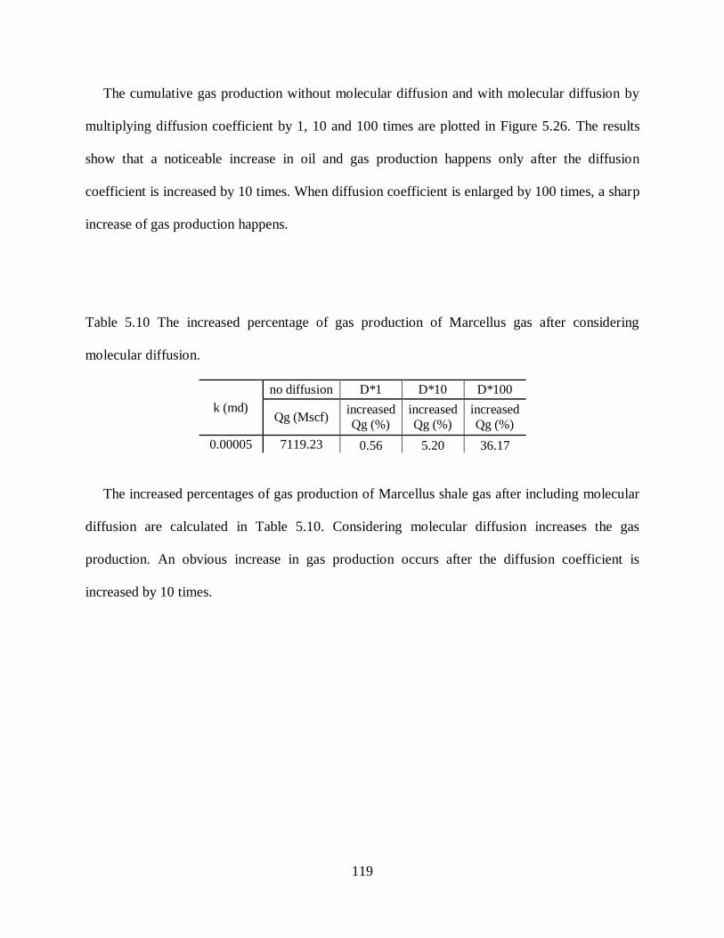
119

The cumulative gas production without molecular diffusion and with molecular diffusion by

multiplying diffusion coefficient by 1, 10 and 100 times are plotted in Figure 5.26. The results

show that a noticeable increase in oil and gas production happens only after the diffusion

coefficient is increased by 10 times. When diffusion coefficient is enlarged by 100 times, a sharp

increase of gas production happens.

Table 5.10 The increased percentage of gas production of Marcellus gas after considering

molecular diffusion.

k (md)

no diffusion D*1 D*10 D*100

Qg (Mscf) increased

Qg (%)

increased

Qg (%)

increased

Qg (%)

0.00005 7119.23 0.56 5.20 36.17

The increased percentages of gas production of Marcellus shale gas after including molecular

diffusion are calculated in Table 5.10. Considering molecular diffusion increases the gas

production. An obvious increase in gas production occurs after the diffusion coefficient is

increased by 10 times.

120

Chapter 6 Conclusions

In this research, first, a black-oil type reservoir simulation method is used to simulate near-

miscible and immiscible produced gas injection enhanced oil recovery. The model allows for gas

injection below and above the critical pressure while black-oil fluid properties are extrapolated

above the original bubble-point pressure. This reduced compositionally black-oil method is

capable of capturing compositional changes of reservoir fluid due to gas injection, and provides a

fast and robust alternative for large-scale reservoir simulation with the purpose of flaring/venting

reduction through reinjecting the produced gas into the reservoir for EOR. Then, the diffusivities

of three types of shale fluids (gas, condensate, crude oil) at reservoir conditions are estimated using

empirical correlations. A gradual increase in CO2 composition in fluid systems accounts for the

gas injection process for EOR/EGR. For the first time, the effect of nano-pores confinement,

including large gas-oil capillary pressure and critical property shifts, on diffusivity is examined.

Meanwhile, the tortuosity factor from laboratory measurements and empirical correlations are used

to characterize the diffusion behavior in porous media. Finally, a fully compositional simulation

model is developed. Nano-confinement effects and molecular diffusion effect are examined on

Bakken oil and Marcellus shale gas production.

6.1 Summary and conclusions

The following conclusions are drawn from this study:

1. In gas flooding schemes, miscible displacement maintains a constant high recovery rate

and reaches maximum recovery in a short period of time; immiscible displacement

maintains the same oil recovery rate but it dramatically decreases after gas breaks through;

121

2. At miscible or near miscible condition, huff-n-puff gas injection is more effective because

more gas dissolves into the oil and dilutes the crude oil;

3. Huff-n-puff gas injection is not effective for the reservoirs that are saturated before gas

injection is started;

4. Using different black oil properties from different gas adding approaches only affects the

results when Pc in flash is included, and the difference is not significant;

5. In tight oil-rich reservoirs, inclusion of high capillary pressure in flash calculation can

significantly increase oil recovery; however, at miscible or near-miscible conditions, the

influence is reduced owing to the low oil-gas IFT;

6. Using IFT-dependent oil-gas relative permeability data can increase the oil recovery in

saturated reservoirs.

7. A validation of empirical correlation indicates that Sigmund correlation is superior to

Wilke‒Chang and Hayduk‒Minhas correlations in terms of predicting the diffusivity of

shale fluid systems at reservoir conditions;

8. The diffusivity of component in gas phase is almost two orders of magnitude larger than in

liquid phase for Bakken oil and is one order of magnitude larger than in liquid phase for

Marcellus shale condensate;

9. For Marcellus shale gas, there is only gas phase at reservoir condition, so no gas-oil

capillary pressure exists. Including critical property shifts could increase CO2 diffusivity

up to 28.0%;

10. For shale condensate, when two phases co-exist, large gas-oil capillary pressure could

decrease the diffusivity in gas phase up to 19.1%, but this reduction in diffusivity

diminishes at higher pressures where single gas phase exists only. Including critical

122

property shifts could slightly decrease the diffusivity in gas phase when two phases co-

exist, but increases diffusivity when single phase gas exists only;

11. For Bakken shale oil, in gas phase, as both nano-confinement effects are included, the

capillary pressure-induced reduction effect on diffusivity is more obvious. In liquid phase,

both capillary pressure effect and critical property shifts increase the diffusivity, but the

effect reduces with continuous CO2 injection;

12. The smaller the pore size is, the more significant the nano-confinement effects on

diffusivity are;

13. Owing to the geometric heterogeneity and complexity of shales, more suitable lithology-

dependent parameters are needed while applying tortuosity-porosity relations to a specific

shale;

14. Based on the shale tortuosity from 3D imaging data, the effective diffusion coefficient in

porous shale rock is reduced by 102–104 times as porosity decreases from 0.1 to 0.03;

15. Including capillary pressure effect increases the oil production but decreases the gas

production; Including critical property shift increase the oil production and slightly

decrease the gas production;

16. The molecular diffusion effect is negligible during Bakken oil or Marcellus shale gas huff-

n-puff production. An obvious increase in oil and gas production happens only after the

diffusion coefficient is multiplied by 10 or 100 times.

123

6.2 Future research

6.2.1 Slim tube simulation to estimate MMP as a function of permeability and fluid

compositions.

One future work is to do the slim tube simulation to estimate MMP as a function of permeability

and composition for different shale oil fluids. Here, the developed fully compositional simulator

will be used. In this work, different solvents (such as CO2, C1, and produced gas) will be injected

into different shale fluids. Meanwhile, the molecular diffusion will be included in the flow

equation. The importance of MMP in very tight shale formation will be investigated. The influence

of permeability, reservoir and injecting gas type, as well as the type of gas drive mass transfer will

be examined.

6.2.2 Inclusion of adsorption behavior in the compositional model to investigate CO2

injection in shale gas in nano-sized pores.

Another future work is to incorporate adsorption behavior in the fully compositional model. Then

we can evaluate the CO2 injection in shale gas reservoir for enhanced gas recovery (EGR) and

greenhouse gas control. Furthermore, confinement effects in shale gas reservoir could be examined

again while considering CO2 adsorption capability and CH4 desorption behavior.

6.2.3 To develop an Embedded Discrete Fracture Model (EDFM).

Another next step to further extend our code to solve more complicated and realistic problems is

to develop an embedded discrete fracture model (EDFM) and couple with the fully compositional

model.

124

APPENDIX A EQUATION OF STATE

Z-factor form of the generalized EOS:

0)]1([)]1()([]1)1[( 2

2121

2

21

2

21

3 BBmmABZBBmmBmmAZBmmZ

(A.1)

where:

c cn

i

n

j

ijji AccA (A.2)

5.0))(1( jiijij AAA (A.3)

2

25.00 )]1(1[ri

ririiaii

T

PTmA (A.4)

cn

i

ii BcB (A.5)

ri

rio

biiT

PB (A.6)

ci

riP

PP (A.7)

ci

riT

TT (A.8)

where ij is the binary interaction coefficient between the component i and j, P is pressure (psia),

T is temperature (R), and v is molar volume (ft3/lbmol)

For SRK EOS

2176.0574.148.0 iiim (A.9)

For PR EOS:

0.49 016666.0164423.048503.1379642.0

0.49 26992.054226.1374640.032

2

iiii

iii

iif

ifm

(A.10)

125

The definition of m1, m2,o

ai , and o

bi for different types of equation of state are is defined as:

Equation of state m1 m2 o

ai o

bi

P-R EOS 21 21 0.457235529 0.077796074

SRK EOS 0 1 0.4274802 0.08664035

126

APPENDIX B VAPOR-LIQUID EQUILIBRIUM

The Rachford-Rice Objective Function is used to solve the gas mole fraction in the mixture

( ngf ).

0)1(1

)1()(

1

cn

i ing

iing

Kf

Kcfg (B.1)

The above equation is a non-linear equation with one known. Generally, Newton Raphson

iterative approach is used to solve the gas fraction ( ngf ).

)(

)(old

ng

old

ngold

ng

new

ngfg

fgff

(B.2)

During this iterative procedure, convergence is achieved as

old

ng

new

ng ff (B.3)

It should be noted that a “negative flash” is implemented by allowing the obtained ngf to be

a negative value and the interval of ngf is:

)1(

1

)1(

1

minmax i

ng

i Kf

K

(B.4)

The compositions component i in liquid phase (xi) and in gas phase (yi) can be calculated as:

)1(1

ing

ii

Kf

cx (B.5)

)1(1

ing

iii

Kf

cKy (B.6)

Newton Raphson method is fast but may lead to an unphysically acceptable range. In that

case, the Bisection method is used. For the Bisection method, the initial upper and lower values

are:

0Ufng ; (B.7)

127

1Lfng; (B.8)

The updated ngf is

LfUff ngng

new

ng (B.9)

The updated upper and lower value becomes:

new

ngng fUf for 0new

ngfg (B.10)

new

ngng fLf for 0new

ngfg (B.11)

Similarly, the iterative procedure stops when

old

ng

new

ng ff (B.12)

128

APPENDIX C PHASE PROPERTIES

C.1 Molecular weight

The molecular weight of vapor and liquid phases are calculated by using weighted average.

n

i

iig MWyMW1

(C.1)

n

i

iil MWxMW1

(C.2)

C.2 Oil and gas densities

The density of phase ‘j’ is calculated by using its phase molecular weight and compressibility

factor ( jZ ) that is predicted from Peng-Robison equation of state.

j

jj

jZ

MW

RT

P (C.3)

C.3 Oil and gas viscosity

C.3.1 Viscosity of gas phase

The viscosity of gas phase is calculated by using the correlation by Lee, Gonzalez and Eakin

(1966), as follows:

vy

g

vvg xEXPk4.62

10 4

(C.4)

Where:

TMW

TMWk

g

g

v

19209

02.04.9 5.1

(C.5)

vv xy 2.04.2 (C.6)

129

gv MWT

x 01.0986

5.3 (C.7)

C.3.2 Viscosity of liquid phase

Lohrenz, Bray and Clark (1964) presented an empirical correlation to predict the viscosity of a

liquid hydrocarbon mixture, is given below:

444321 100093324.0040758.0058533.0023364.01023.0 rrrrml (C.8)

l is the liquid viscosity (cp); m is the viscosity at atmospheric pressure(cp-1); r is the reduced

liquid density, and is the viscosity at atmospheric pressure (cp) and is calculated by Herning

& Zipperer equation.

i

ii

i

iii

MWx

MWx

(C.9)

i is the viscosity of component i at low pressure and is suggested by Stiel and Thodos.

5.1 )67.158.4(78.17

5.1 10.34

625.05

94.05

TriforT

TriforT

i

ri

i

ri

i

(C.10)

i is the viscosity parameter of the i-th component given by:

3/2

6/14402.5

pci

pc

iPMW

T (C.11)

pcT is the pseudocritical temperature (R); pcP is the pseudocritical pressure (psia); MWl is the

molecular weight of the liquid phase (lbm/lbmol).

The reduced density of liquid mixture ( r ) is calculated from Lohrentz et al. (1969):

130

pc

l

l

pc

lr V

WM

(C.12)

pc is the pseudocritical density of the liquid phase(lbm/ft3) and Vpc is the pseudocritical volume

of the liquid per unit mole (ft3/lbmol). All mixture pseudocritical properties are calculated using

Kay’s mixing rule, as below:

ciipc TxT (C.13)

ciipc PxP (C.14)

ciipc VxV (C.15)

C.4 Saturation

Gas saturation in reservoir can be calculated from vapor and liquid mole fractions by flash

calculation. Oil saturation can be obtained based on the fact that the sum of oil, gas, and water

saturation is equal to 1.

onggng

gng

w

onogng

gng

w

og

g

wgvfvf

vfS

vfvf

vfS

VV

VSS

)1(111

(C.16)

owg SSS 1 (C.17)

C.5 Water properties

The density of water is calculated as:

)(1 ,refwww

o

ww PPC (C.18)

131

References

Adel, I.A.; Tovar, F.D.; Zhang, F.; Schechter, D.S., 2018. The impact of MMP on recovery factor

during CO2−EOR in Unconventional liquid reservoirs. In Proceedings of the Paper SPE

191752 Present at the SPE Annual Technical Conference and Exhibition, San Antonio, Texas,

USA, 24–26 September.

Alharthy, N., Teklu, T., Kazemi, H., Graves, R., Hawthorne, S., Braunberger, J., Kurtoglu, B.,

2017. Enhanced oil recovery in liquid-rich shale reservoirs: laboratory to field. SPEREE

21(01), 137−159.

Atan, S.; Ajayi, A.; Honarpour, M.; Turek, E.; Dillenbeck, E.; Mock, C.; Ahmadi, M.; Pereira, C.,

2018. The viability of gas injection EOR in Eagle Ford shale reservoirs. In Proceedings of the

Paper SPE 191673 Present at the SPE Annual Technical Conference and Exhibition, San

Antonio, TX, USA, 24–26 September.

Atkins, E.R., Smith, G.H., 1961. The significance of particle shape in formation resistivity factor-

porosity relations. J. Petroleum Technol., 13, 285–291.

Ayirala, S.C., Rao, D.N., 2006. A new parachor model to predict dynamic interfacial tension and

miscibility in multicomponent hydrocarbon systems. J. Colloid Interf. Sci. 299(1): 321−331.

Backeberg, N.R., Lacoviello, F., Rittner, M., Mitchell, T.M., Jones, A.P., Day, R, Wheeler, J.,

Shearing, P.R., Vermeesch, P., Striolo, A., 2017. Quantifying the anisotropy and tortuosity of

permeable pathways in clay-rich mudstones using models based on X-ray tomography. Sci.

Rep. 7, 14838.

Blom, S.M.P., Hagoort, J., 1998. How to include the capillary number in gas condensate relative

permeability Functions? SPE Paper 49268 Presented at the SPE Annual Technical Conference

and Exhibition, 27−30 September, New Orleans, Louisiana, USA.

132

Boudreau, B.P., 1996. The diffusive tortuosity of fine-grained unlithified sediments. Geochim.

Cosmochim. Acta. 60, 3139–3142.

Bruggeman, V.D. (1935). Berechnung verschiedener physikalischer konstanten von heterogenen

substanzen. I. dielektrizitätskonstanten und leitfähigkeiten der mischkörper aus isotropen

substanzen. Ann Phys. 416, 636–664.

Bullin, K., Krouskop, P., 2008. Composition variety complicates processing plans for US shale

gas. Based on a presentation to the Annual Forum, Gas Processors Association–Houston

Chapter, October 7.

Chalmers, G.R., Bustin, R.M., Power, I.M., Characterization of gas shale pore systems by

porosimetry, pycnometry, surface area, and field emission scanning electron

microscopy/transmission electron microscopy image analyses: Examples from the Barnett,

Woodford, Haynesville, Marcellus, and Doig units. AAPG BULL. 96, 1099–1119.

Chen, C.; Balhoff, M.; Mohanty, K.K., 2013. Effect of reservoir heterogeneity on improved shale

oil recovery by CO2 huff-n-puff. In Proceedings of the Paper SPE 164553 Presented at the

Unconventional Resources Conference, The Woodland, TX, USA, 10–12 April.

Chen, C.; Balhoff, M.; Mohanty, K.K., 2014. Effect of reservoir heterogeneity on primary recovery

and CO2 huff ‘n’ puff recovery in shale-oil reservoirs. SPEREE 17, 404–413.

Chen, C., Hu, D., Westacott, D., Loveless, D., 2013. Nanometer-scale characterization of

microscopic pores in shale kerogen by image analysis and pore-scale modeling. Geochem.

Geophy. Geosy.14(10), 4066–4075.

Chen, L., Zhang, L., Kang, Q., Viswanathan, H.S., Yao, J., Tao, W., 2015. Nanoscale simulation

of shale transport properties using the Lattice Boltzmann method: permeability and diffusivity.

Sci. Rep. 5, 8089.

133

Coats, K., 1980, An equation of state compositional model. SPE J 20(5), 363−76.

Cooper, S.J., Bertei, A., Shearing, P.R., Kilner, J.A., Brandon, N.P., 2016. An open-source

application for calculating tortuosity factors from tomographic data. SoftwareX 5, 203−210.

da Silva, F.V., Belery, P., 1989. Molecular diffusion in naturally fractured reservoirs: A decisive

recovery mechanism. SPE 19672. Presented at the 64th SPE Fall Meeting, San Antonio, TX.

October 8−11.

Dong C., Hoffman B.T. Modeling gas injection into shale oil reservoirs in the Sanish field, North

Dakota, presented at Unconventional Resources Technology Conference, 12-14 August,

Denver, Colorado, 2013.Du, F., Nojabaei, B., 2019. A review of gas injection in shale

reservoirs: enhanced oil/gas recovery approaches and greenhouse gas control. Energies 12(12),

2355.

Du, F., Ma, H., Gu, Y., 2019. Three different periods of CO2 dissolution into a light crude oil. Can.

J. Chem. Eng. 97, 330–43.

Du, F., Huang, J., Chai, Z., Killough, J., 2020. Effect of vertical heterogeneity and nano-

confinement on the recovery performance of ooil-rich shale reservoir. Fuel. 267, 117199.

Du, F.; Nojabaei, B., 2020. A black-oil approach to model produced gas injection in both

conventional and tight oil-rich reservoirs to enhance oil recovery. Fuel, 263(1), 116680.

Du, F.; Nojabaei, B., 2019. A review of gas injection in shale reservoir: enhanced oil/gas recovery

approaches and greenhouse gas control. Energies. 12(12), 2355.

Du, F.; Nojabaei, B., 2020. Estimating diffusion coefficients of shale oil, gas, and condensate with

nano-confinement effect. J. Pet. Sci. Eng. 193, 107362.

Dysthe, D.K., Hafskjold, B., 1995. Inter- and intradiffusion in liquid mixtures of methane and n-

decane. Int. J. Thermophys. 16, 1213–1224.

134

Energy Information Administration (EIA). Even as Renewables Increase, Fossil Fuels Continue to

Dominate U.S. Energy Mix. 2017. Available online:

https://www.eia.gov/todayinenergy/detail.php?id=31892 .

Energy Information Administration (EIA). Technically Recoverable Shale Oil and Shale Gas

Resources: An Assessment of 137 Shale Formations in 41 Countries outside the United States.

2013. Available online:https://www.eia.gov/analysis/studies/worldshalegas/pdf/overview.pdf

Energy Information Administration (EIA). Future U.S. Tight Oil and Shale Gas Production

Depends on Resources, Technology, Markets. 2016. Available online:

https://www.eia.gov/todayinenergy/detail.php?id=27612.

Elamin, A., 2013. Simulation of multi-component gas flow and condensation in Marcellus shale

reservoir. Master thesis.

Epstein, N., 1989. On tortuosity and the tortuosity factor in flow and diffusion through porous

media. Chem. Eng. Sci. 44,777–779.

Fathi, E.; Akkutlu, I.Y., 2012. Mass transport of adsorbed-phase in stochastic porous medium with

fluctuating porosity field and nonlinear gas adsorption kinetics. Transp. Porous Med. 91, 5‒

33.

Fathi, E., Akkutlu, I.Y., 2014. Multi-component gas transport and adsorption effects during CO2

injection and enhanced shale gas recovery. Int. J. Coal. Geol. 123, 52−61.

Gamadi, T.D.; Sheng, J.J.; Soliman, M.Y. An experimental study of cyclic gas injection to improve

shale oil recovery. In Proceedings of the Paper SPE 166334 Presented at the SPE Annual

Technical Conference and Exhibition, New Orleans, LA, USA, 30 September–2 October 2013.

Gamadi, T.D.; Elldakli, T.F.; Sheng, J.J., 2014a. Compositional simulation evaluation of EOR

potential in shale oil reservoirs by cyclic natural gas injection. In Proceedings of the URTeC

135

1922690 Presented at the Unconventional Resources Technology Conference, Denvor, CO,

USA, 25–27 August.

Gamadi, T.D.; Sheng, J.J.; Soliman, M.Y.; Menouar, H.; Watson, M.C.; Emadibaladehi, H.,

2014b. An experimental study of cyclic CO2 injection to improve shale oil recovery. In

Proceedings of the Paper SPE 169142 Presented at the SPE Improved Oil Recovery

Symposium, Tulsa, OK, USA, 12–16 April.

Gao, Z.; Hu, Q., 2013. Estimating permeability using median pore-throat radius obtained from

mercury intrusion porosimetry. J Geophy Eng 2013;10:1‒7.

Gottwald, A., Creamer, L.K., Hubbard, P.L., Callaghan, P.T., 2005. Diffusion, relaxation, and

chemical exchange in casein gels: A nuclear magnetic resonance study. J. Chem. Phys. 122,

034506.

Hayduk, W., Minhas, B.S., 1982. Correlations for prediction of molecular diffusivities in liquids.

Hoffman, B.T., 2012. Comparison of various gases for enhanced recovery from shale oil

reservoirs. In Proceedings of the Paper SPE 154329 Presented at the Eighteenth SPE Improved

Oil Recovery Symposium, Tulsa, OK, USA, 14–18 April.

Hoffman, B.T.; Evans, J.G. Improved oil recovery IOR pilot projects in the Bakken formation. In

Proceedings of the Paper SPE 180270 Presented at the SPE Low Perm Symposium, Denver,

CO, USA, 5–6 May 2016.

Huang, J., Jin, T., Chai, Z., Barrufet, M., Killough, J., 2019a. Compositional simulation of

fractured shale reservoir with distribution of nanopores using coupled multi-porosity and

EDFM method. J. Pet. Sci. Eng. 179, 1078−1089.

Huang, J., Xiao, F., Dong, H., Yin, X., 2019b. Diffusion tortuosity in complex porous media from

pore-scale numerical simulations. Comput. Fluids 185, 66−74.

136

Huang, J., Jin, T., Chai, Z., Barrufet, M., Killough J., 2020. Compositional simulation of three-

phase flow in mixed-wet shale oil reservoir. Fuel 260, 1–11.

Iversen, N., Jorgensen, B.B., 1993. Diffusion coefficients of sulfate and methane in marine

sediments: influence of porosity. Geochim. Cosmochim. Acta. 25, 327–337.

Jessen, K.; Orr, F.M., 2008. On interfacial-tension measurements to estimate minimum miscibility

pressures. SPEREE 11, 933–939.

Jiang, J., Younis, R.M., 2016. Compositional modeling of enhanced hydrocarbons recovery for

fractured shale gas-condensate reservoirs with the effects of capillary pressure and

multicomponent mechanisms. J. Nat. Gas Sci. Eng. 34, 1262−1275.

Jin, L.; Hawthorne, S.; Sorensen, J.; Pekot, L.; Bosshart, N.; Gorecki, C.; Steadman, E.; Harju, J.,

2017a. Utilization of produced gas for improved oil recovery and reduced emissions from the

Bakken formation. In Proceedings of the Paper SPE 184414 Presented at the SPE Health,

Safety, Security, Environment, & Social Responsibility Conference, New Orleans, LA, USA,

18–20 April.

Jin, L.; Hawthorne, S.; Sorensen, J.; Pekot, L.; Kurz, B.; Smith, S.; Heebink, L.; Bosshart, N.;

Torres, J.; Dalkhaa, C. 2017b Extraction of oil from the Bakken shales with supercritical CO2.

In Proceedings of the Paper SPE 2671596 (URTEC 2671596) Presented at SPE/AAPG/SEG

Unconventional Resources Technology Conference, Austin, TX, USA, 24–26 July.

Kalantari-Dahaghi, A. Numerical simulation and modeling of enhanced gas recovery and CO2

sequestration in shale gas reservoirs: A feasibility study. In Proceedings of the Paper SPE

139701 Presented at the SPE International Conference on CO2, Capture, Storage, and

Utilization, New Orleans, LA, USA, 10–12 November 2010.

137

Kalla, S., Leonardi, S.A., Berry, D.W., Poore, L.D., Sahoo, H., Kudva, R.A., Braun, E.M., 2015.

Factors that affect gas-condensate relative permeability. SPEREE 8(1), 5‒10.

Lerman, A., 1979. Geochemical Processes: Water and sediment environments. Wiley, New York.

Li, L.; Su, Y.; Sheng, J.J.; Hao, Y.; Wang, W.; Lv, Y.; Zhao, Q.; Wang, H., 2019. Experimental

and numerical study on CO2 sweep volume during CO2 huff-n-puff enhanced oil recovery

process in shale oil reservoirs. Energy Fuels, 33, 4017–4032.

Low, P.F., 1981. Principles of ion diffusion in clays. In: Chemistry in the Soil Environment,

American Society for Agronomy, Special Publication, 40, 31–45.

Macleod, D.B., 1923. On a relation between surface tension and density, Trans. Faraday Soc. 19,

38–42.

Matyka, M., Khalili, A., Koza, Z., 2008. Tortuosity-porosity relation in porous media flow. Phys.

Rev. E Stat. Nonlinear Soft Matter Phys. 78, 1–8.

Meng, X.; Sheng, J.J.; Yu, Y., 2017. Experimental and numerical study of enhanced condensate

recovery by gas injection in shale gas−condensate reservoirs. SPEREE 20, 471–477

Morishige, K., Fujii, H., Uga, M., Kinukawa, D., 1997. Capillary critical point of argon, nitrogen,

oxygen, ethylene, and carbon dioxide in MCM-41. Langmuir, 13, 3494‒3498.

Nghiem, L.X., Kohse, B.F., Sammon, P.H., 2001. Compositional simulation of the VAPEX

process. J. Can. Pet. Technol., 40(4), 41‒48.

Nojabaei, B., Johns, R.T, Chu, L., 2013. Effect of Capillary Pressure on Phase Behavior in Tight

Rocks and Shales, SPEREE, 16(3), 281−289.

Nojabaei, B., Johns, R.T, 2016. Extrapolation of black- and volatile-oil fluid properties with

application to immiscible/miscible gas injection. J. Nat. Gas Sci. Eng. 33, 367−37.

138

Nojabaei, B., Johns, R.T, Chu, L., 2013. Effect of Capillary Pressure on Phase Behavior in Tight

Rocks and Shales. SPEREE 16(3), 281−89.

Pederson K.S., Christensen, P.L., 2007. Phase behavior of petroleum reservoir fluids. CRC Press,

Taylor & Francis Group.

Peng, D.Y. and Robinson, D.B., 1976. A New Two-Constant Equation of State. Industrial and

Engineering Chemistry Fundamentals 15(1), 59-64.

Peng, S., Yang, J., Xiao, X., Loucks, B., Ruppel, S.C., Zhang, T., 2015. An integrated method for

upscaling pore-network characterization and permeability estimation: example from the

Mississippian Barnett Shale. Transp. Porous Med. 109, 359–376.

Petersen, E.E., 1958. Diffusion in a pore of varying cross section. AICHE J. 4, 343–345.

Prenni, A.J.; Day, D.E.; Evanoski-Cole, A.R.; Sive, B.C.; Hecobian, A.; Zhou, Y.; Gebhart, K.A.;

Hand, J.L.; Sullivan, A.P.; Li, Y.; et al., 2016. Oil and gas impacts on air quality in federal

lands in the Bakken region: An overview of the Bakken air quality study and first results.

Atmos. Chem. Phys. 16, 1401–1416.

Ratner, M.; Tiemann, M., 2018. An Overview of Unconventional Oil and Natural Gas: Resources

and Federal Actions. Congressional Research Service Report. 2015. Available online:

https://fas.org/sgp/crs/misc/R43148.pdf.

Reid, R.C., Prausnitz, J.M., Poling, B.E., 1987. The properties of gases and liquids (4th edition).

MCgRAW Hill Book Co, New York, NY.

Sanchez-Rivera, D.; Mohanty, K.; Balhoff, M., 2015. Reservoir simulation and optimization of

huff-n-puff operations in the Bakken shale. Fuel 147, 82–94.

Shabro, V., Kelly, S., Torres-Verdin, C., Sepehrnoori, K., 2013. Pore-scale modeling of electrical

resistivity and permeability in FIB-SEM images of hydrocarbon-bearing shale. Presented:

139

SPWLA 54th Annual Logging Symposium. Society of Petrophysicists and Well-Log Analysts,

New Orleans, Louisiana, June 22−26.

Shen, L., Chen, Z., 2007. Critical review of the impact of tortuosity on diffusion. Chem. Eng. Sci.

62, 3748−3755.

Sheng, J.J., 2015. Enhanced oil recovery in shale reservoirs by gas injection. J. Nat. Gas Sci. Eng.

22, 252–259.

Sheng, J.J.; Chen, K., 2014. Evaluation of the EOR potential of gas and water injection in shale

oil reservoirs. J. Unconv. Oil Gas Resour. 5, 1–9.

Shoaib S., Hoffman B.T., 2009. CO2 flooding the Elm Coulee field, presented at SPE Rocky

Mountain Petroleum Technology Conference, Denver, Colorado.

Sigmund, P.M., 1976. Prediction of molecular diffusion at reservoir conditions. Part I‒

measurement and prediction of binary dense gas diffusion coefficients. J. Can. Pet. Technol.

15, 48‒57.

Sigmund, P.M., 1976. Prediction of molecular diffusion at reservoir conditions. Part II‒estimating

the effects of molecular diffusion and convective mixing in multi-component systems. 15, 53‒

62.

Siripatrachai, N., 2016. Development of A Multi-mechanistic Triple-porosity, Triple-permeability

Compositional Model for Unconventional Reservoirs. Dissertation.

Song, L., Kantzas, A., Bryan, J. Experimental Measurement of Diffusion Coefficient of CO2 in

Heavy Oil Using X-Ray Computed-Assisted Tomography under Reservoir Conditions. Paper

SPE 137545, presented at the Canadian Unconventional Resources and International

Petroleum Conference, Calgary, Alberta, October 19–20, 2010.

140

Song, C., Yang, D., 2017. Experimental and numerical evaluation of CO2 huff-n-puff processes

in Bakken formation. Fuel 190, 145−62.

Steptoe, A.P., Carr, T.R., 2011. Lithostratigraphy and Depositional systems of the Bakken

formation in the Williston Basin, North Dakota. Poster presentation at AAPG Eastern Section

Meeting, Kalamazoo, Michigan, September 25–29.

Stone, H.L., 1973. Estimation of three-phase relative permeability and residual oil data. J. Can.

Pet. Technol. 12(4), 52−61.

Sugden, S., 1924.The variation of surface tension with temperature and some related functions, J.

Chem. Soc. 32–41.

Sun, H., Yao, J., Cao, Y., Fan, D., Zhang, L., 2017. Characterization of gas transport behaviors in

shale gas and tight gas reservoirs by digital rock analysis. Int. J. Heat Mass Transfer 104, 227–

239.

Sun, J., Zou, A., Sotelo, E., Schechter, D., 2016. Numerical simulation of CO2 huff-n-puff in

complex fracture networks of unconventional liquid reservoirs. J. Nat. Gas Sci. Eng. 31,

481−492.

Tahmasebi, P., Javadpour, F., Sahimi, M., Piri, M., 2016. Multiscale study for stochastic

characterization of shale samples. Adv. Water Resour. 89, 91–103.

Teklu, T.W., Alharthy, N., Kazemi, H., Yin, X., Graves, R.M., AlSumaiti, A.M., 2014. Phase

behavior and minimum miscibility pressure in nanopores. SPEREE, 17(3), 396–403.

Tjaden, B., Cooper, S.J., Brett, D.J., Kramer, D., Shearing, P.R., 2016. On the origin and

application of the Bruggeman correlation for analysing transport phenomena in

electrochemical systems. Curr. Opin. Chem. Eng. 12, 44–51.

141

Todd, M.R., Longstaff, W.J., 1972. The development, testing, and application of a numerical

simulator for predicting miscible flood performance. JPT 24 (7): 874‒82.

Ullman, W.J., Aller, R.C., 1982. Diffusion coefficients in near shore marine sediments. Limnol.

Oceanogr. 27, 552–556.

Wan, T.; Yu, Y.; Sheng, J.J., 2015. Experimental and numerical study of the EOR potential in

liquid-rich shales by cyclic gas injection. J. Unconv. Oil Gas Resour. 12, 56–67.

Wang, S., Ma, M., Chen, S., 2016. Application of PC-SAFT equation of state for CO2 minimum

miscibility pressure prediction in nanopores. SPE Paper 179535 Presented at the SPE

Improved Oil Recovery Conference, 11−13 April, Tulsa, Oklahoma, USA.

Wang, H., Wang, X., Jin, X., Cao, D., 2016. Molecular dynamics simulation of diffusion of shale

oils in montmorillonite. J. Phys. Chem. C 120, 8986‒8991.

Weinaug, C.F. and Katz, D.L., 1943.Surface tensions of methane–propane mixtures, Ind. Eng.

Chem. 35, 239–246.

Weissberg, H., 1963. Effective diffusion coefficients in porous media. J. Apply. Phys. 34, 2636–

2639.

Wilke, C.R., 1950. Diffusional properties of multicomponent gases. Chem. Eng. Progress 46, 95–

104

Wilke, C.R., Chang, P., 1955. Correlation of diffusion coefficients in dilute solutions. AIChE J. 1,

264‒270.

Yang, D.Y.; Song, C.; Zhang, J.; Zhang, G.; Ji, Y.; Gao, J., 2015. Performance evaluation of

injectivity for water-alternating-CO2 processes in tight oil formations. Fuel 139, 292–300.

Yu, W., Lashgari, H.R., Wu, K., Sepehrnoori, K., 2015. CO2 injection for enhanced oil recovery

in Bakken tight oil reservoirs. Fuel. 159(1), 354−363.

142

Yu, W., Lashgari, H., Sepehrnoori, K., 2014. Simulation study of CO2 huff-n-puff process in

Bakken tight oil reservoirs. In: SPE Paper 169575 Presented at SPE Western North American

and Rocky Mountain Joint Meeting, 17−18 April, Denver, Colorado.

Yu, W.; Zhang, Y.; Varavei, A.; Sepehrnoori, K.; Zhang, T.; W, K.; Miao, J., 2018. Compositional

simulation of CO2 huff-n-puff in Eagle Ford tight oil reservoirs with CO2 molecular diffusion,

Nano pore confinement and complex natural fractures. In Proceedings of the Paper SPE

190325 Presented at the SPE Improved Oil Recovery Conference, Tulsa, OK, USA, 14–18

April.

Yu, Y.; Li, L.; Sheng, J.J. A comparative experimental study of gas injection in shale plugs by

flooding and huff-n-puff processes. J. Nat. Gas Sci. Eng. 2017, 38, 195–202.

Zarragoicoechea, G., Kuz, V.A., 2004. Critical shift of a confined fluid in a nanopore. Fluid Phase

Equilib. 220, 7‒9.

Zhang, Y., Di, Y., Yu, W., Sepehrnoori, K., 2017. A Comprehensive Model for Investigation of

CO2-EOR with Nanopore Confinement in the Bakken Tight Oil Reservoir. In: Paper SPE

187211 Presented at SPE Annual Technical Conference and Exhibition, 9–11 October, San

Antonio, Texas, USA.

Zhang, Y.; Yu, W.; Li, Z.; Sepehrnoori, K., 2018 Simulation study of factors affecting CO2 huff-

n-puff process in tight oil reservoirs. J. Pet. Sci. Eng. 163, 264–269. 51.

Zhang, K.; Nojabaei, B.; Ahmadi, K.; Johns, R.T., 2018. Minimum miscibility pressure calculation

for oil shale and tight reservoirs with large gas–oil capillary pressure. In Proceedings of the

URTeC 2901892 Presented at the Unconventional Resources Technology Conference,

Houston, TX, USA, 23–25 July. 59.

143

Zuloaga, P.; Yu, W.; Miao, J.; Sepehrnoori, K., 2017. Performance evaluation of CO2 huff-n-puff

and continuous CO2 injection in tight oil reservoirs. Energy 134, 181–192.