in pursuit of a long term record of erosion rates from the...
TRANSCRIPT

In Pursuit of a Long Term Record of Erosion Rates from the Río Iruya Canyon, Northwestern Argentine Andes
by
Lisa Luna
Submitted in partial fulfillment of
the requirements for the degree of
Bachelor of Arts
Department of Geology
Middlebury College
Middlebury, Vermont
May, 2013
ii
Luna, Lisa V., 2013. In pursuit of a long term record of erosion rates from the Río Iruya Canyon, Northwestern Argentine Andes. Unpublished senior thesis, Middlebury College, Middlebury, VT.
ABSTRACT
The relationship between climate, tectonics, and erosion rates in mountainous terrain remains poorly understood over long timescales. Although studies of modern systems allow comparison across modern climatic and tectonic gradients, long-term records are required to test the importance of disequilibrium landscape conditions created by global climate cycles and long-term climate trends. The Río Iruya canyon in the northwestern Argentine Andes is an exceptional location to develop a long-term record of erosion rates using cosmogenic 10Be. The 100-m deep canyon is an extraordinary section of ~7500 m of sedimentary rock deposited in the Andean foreland basin during growth of the sub-Andean fold and thrust belt and only recently re-exposed when the river overwhelmed a flood control canal in 1898. Minimal post-burial cosmogenic production, along with published paleomagnetic stratigraphy data, makes the canyon an ideal location to study erosion rate response to changes in tectonic activity and climate cycling. We present a high-resolution record of temporal variations in paleo-erosion rates from cosmogenic 10Be in the Río Iruya watershed that suggests that erosion rates responded to changes in the orbitally controlled South American Summer Monsoon between 3.4 and 2.5 Ma, and to regional tectonic uplift between 2.5 and 1 Ma. To refine the current canyon stratigraphic framework, this study presents LA-ICPMS U-Pb zircon dates from three previously undated interbedded ashes at 7.01 +0.10/-0.04 Ma, 4.07 +0.07/-0.03 Ma, and 2.77 +0.05/-0.06 Ma. We constrain sedimentary provenance and interpret watershed evolution through kernel density estimation plots from two modern and four paleo-detrital zircon samples.

iii
ACKNOWLEDGEMENTS First and foremost, I want to thank my advisor, Will Amidon, for involving me in this project and for the many hours he has spent teaching me to be a better scientist. Working on this project has truly been one of the most rewarding experiences of my Middlebury career. Burch Fisher, for his humorous support through all night food poisoning, all night zircon dating, and all day cliff top driving and for doing all of the beryllium chemistry. Doug Burbank, for kind geological explanations of everything from strath terraces to geomagnetic fields, and for encouragement along the way. I want to thank my parents, Larry and Rachelle Luna, for always being so supportive of me through my whole life and thesis project, and for funding my Middlebury College education. It looks like I’m going to turn out a scientist after all. The Middlebury College Geology department for teaching me so many things over these four years, many of which I’ve applied to this thesis, and in particular Jeff Munroe, for roping me into this whole geology business in the first place. My fellow geology seniors, who have provided all kinds of support over the course of the last year. In particular, I want to thank Juliet Ryan-Davis for late night dance parties in the lab, for explaining zircon when things were looking grim, and for bringing good cheer. Emma Loizeaux, for eagerly listening to me ramble endlessly about cosmogenic beryllium, rant about my data, and for being my best friend. Sarina Patel, Kris Falcones, Abra Atwood, and Nick Orr for their hard work in the lab. I wouldn’t have been able to pull this off without your help. Andrew Kylander-Clark, for hard work fixing the LA-ICPMS, and for reducing the U-Pb data. Ray Coish, for help running the ICP, and Dan Ruscitto, for help with CL-images. Chris Johnson, for keeping me happy and for helping to keep things in perspective. Funding for this project was provided by the NSF.

iv
TABLE OF CONTENTS
ABSTRACT ................................................................................................................... ii ACKNOWLEDGEMENTS ........................................................................................... iii TABLE OF CONTENTS ............................................................................................... iv
LIST OF FIGURES ....................................................................................................... vi LIST OF TABLES ....................................................................................................... vii CHAPTER I ....................................................................................................................1
1. Introduction .............................................................................................................1
2. Background .............................................................................................................3
Erosion Rates ...........................................................................................................3
Determining Erosion Rates with Cosmogenic Isotopes.............................................6
Previous Work with Basin Scale Erosion Rates ........................................................9
Zircon Geochronometry and Provenance Studies ................................................... 11
3. Study Area ............................................................................................................. 13
Tectonic Setting of the Modern Río Iruya Watershed ............................................. 13
Bedrock Geology of the Modern Río Iruya Watershed ........................................... 15
Climatic Setting of the Subandes and Cordillera Oriental ....................................... 17
The Río Iruya Section ............................................................................................ 18
CHAPTER II ................................................................................................................. 23
1. Field Methods ........................................................................................................ 23
Sediment Collection for Cosmogenic 10Be and Ash Collection for Zircon Dates .... 23
2. Laboratory Methods ............................................................................................... 24
Quartz Purification ................................................................................................. 24
Quartz Purity Testing ............................................................................................. 25
Beryllium Extraction Chemistry ............................................................................. 26
Measuring 10Be with AMS ..................................................................................... 27
Ash Zircon Separation ........................................................................................... 28
Detrital Zircon Separation ...................................................................................... 29
Cathodoluminescence Imaging .............................................................................. 30
U-Pb Dating with LA-MC-ICPMS ......................................................................... 31
3. Analytical Methods ................................................................................................ 33

v
Tuff Age Determination from Single Grain LA-ICPMS 238U/206Pb and 207Pb/206 Dates ..................................................................................................................... 33
Detrital Zircon Ages and Kernel Density Estimation Plots ..................................... 34
Erosion Rate Determination from 10Be Concentration ............................................ 34
CHAPTER III ................................................................................................................ 38
1. Results ................................................................................................................... 38
Ash Zircon Ages .................................................................................................... 38
Detrital Zircon Age Distributions ........................................................................... 39
Cosmogenic 10Be Erosion Rate Estimates .............................................................. 41
CHAPTER IV ............................................................................................................... 42
1. Discussion ............................................................................................................. 42
Improved Age Model for the Río Iruya Section ...................................................... 42
Provenance Changes in the Río Iruya Watershed ................................................... 44
Evolution of the Río Iruya Watershed .................................................................... 48
Implications for Erosion Rate Calculations ............................................................ 49
Comparison of Erosion Rates with Proxies............................................................. 49
Recommendations for Continued Work in the Watershed ...................................... 51
REFERENCES .............................................................................................................. 53
APPENDICES ............................................................................................................... 57
Appendix A. LA-ICPMS U-Pb Zircon Data and Tuff Ages .................................... 57
Appendix B. AMS 10Be data and conversions ........................................................ 57
Appendix C. MATLAB code used to calculate erosion rates .................................. 57
Appendix D. Erosion rate estimates ....................................................................... 57

vi
LIST OF FIGURES Figure 1. Study area in context of Andean provinces……………………………………..2
Figure 2. δ18O record for the past 5 Ma…………………………………………………...6
Figure 3. 238U to 206Pb decay scheme……………………………………………………12
Figure 4. Structural growth of the Subandes…………………………………………….15
Figure 5. Bedrock geology of the Río Iruya watershed………………………………….16
Figure 6. Regional precipitation…………………………………………………………18
Figure 7. Previously published magnetostratigraphy…………………………………….20
Figure 8. Sampling locations in the Río Iruya canyon…………………………………...21
Figure 9. Cathodoluminescence image of ash zircons…………………………………..30
Figure 10. Modern detrital zircon sampling locations…………………………………..31
Figure 11. Sediment accumulation rates for the Río Iruya section………………………37
Figure 12. Detrital zircon kernel density estimates……………………………………..40
Figure 13. Tuff ages and reinterpreted magnetostratigraphy……………………………43
Figure 14. Evolution of the Río Iruya watershed………………………………………...47
Figure 15. Erosion rates and climate proxies…………………………………………….50
vii
LIST OF TABLES Table I. Cosmogenic 10Be samples and depositional ages……………………………….23
Table II. Tuff samples, zircon statistics, and ages……………………………………….38
Table III. Detrital samples, zircon statistics, and depositional ages…………………….39
Table IV. Cosmogenic 10Be erosion rate estimates……………………………………...41
1
CHAPTER I
1. Introduction
The interaction between climate, tectonics, and erosion rates has long been a
fundamental geological mystery (e.g. Molnar and England, 1990). Researchers working
at individual sites around the world have alternately discovered that climate drives
erosion rates, that tectonics drive erosion rates, and that erosion rates drive climate and
tectonics (e.g. Bookhagen and Strecker, 2012; Safran et al., 2005; Raymo and Ruddiman,
1992). For longer time scales, high quality records of erosion rates are necessary to help
untangle these complex interactions. Previous studies have used sedimentation rates as a
proxy for erosion rates over time (Zhang et al., 2001), and many have noted an increase
in the rate of sedimentation in the past 5 Ma (Hay et al., 1988). Zhang et al. (2001) have
interpreted this as an increase in erosion rates caused by larger amplitude and higher
frequency climate oscillations that began at approximately 3 Ma (Zachos et al., 2001).
Unfortunately, sedimentation rates are an unwieldy proxy for erosion rates
(Molnar, 2004). A preferable method is to determine erosion rates using cosmogenic
isotopes. By analyzing cosmogenic isotopes in surface rocks or stream sediment,
researchers have been able to directly estimate erosion rates from outcrop to basin scales
(Granger et al., 1996).
Cosmogenic isotopes are most commonly used to estimate erosion rates for
modern basins. However, the technique has recently been expanded to ancient basins by
estimating erosion rates from sedimentary rocks that were deposited in ancient fluvial
systems (Charreau et al., 2011). Cosmogenic isotope studies of paleo-erosion rates have

2
the potential to produce the high quality long-term record necessary to disentangle the
interactions between climate, tectonics, and erosion rates over time.
The Río Iruya canyon in the Central Andes of Northwestern Argentina is an ideal
place to develop a record of paleo-erosion rates using cosmogenic isotopes because it
contains a fluvially deposited and recently re-exposed sedimentary section with an
independently determined chronology (Figure 1). The Río Iruya overwhelmed a flood
control canal in 1898 and began incising its present canyon, exposing approximately
7500 m and 11 Ma of continuous sedimentary section that has been dated using
magnetostratigraphy and tephrachronology (Hernández et al., 1996).
Figure 1. Location of the modern Río Iruya watershed in the context of the Andean morphotectonic provinces.

3
This study focuses on the relationship between erosion rates, long-term climate
cycling, and tectonic activity in the Río Iruya watershed. Using cosmogenic 10Be derived
from 3.4 to 1 million year old quartz-bearing strata, this study presents a high-resolution
time series of erosion rates in the Río Iruya catchment during the transition from a more
stable to a more variable global climate. Our preliminary erosion rate estimations suggest
that erosion rates responded to changes in the orbitally controlled South American
Summer Monsoon between 3.4 and 2.5 Ma, and to regional tectonic uplift between 2.5
and 1 Ma. This study also improves Hernández et al. (1996)’s age control with new
magnetostratigraphy data and U-Pb zircon ages for 5 interbedded ashes for improved
correlation with climate proxies and better erosion rate estimates. Additionally, it uses
detrital zircons to track provenance changes in the section and better understand the
evolution of and tectonic activity in the watershed over time.
2. Background
Erosion Rates
Erosion is the process by which geomorphic agents remove mechanically and
chemically weathered rock from a surface (Burbank and Anderson, 2001). There are
many factors that control where and how quickly erosion happens, and they vary over
temporal and spatial scales. Some of these factors are precipitation, topography, presence
or absence of glaciers, type and distribution of vegetation, and bedrock lithology.
At a regional scale, two processes control rates of erosion. The first is crustal
deformation, which provides potential energy to the major erosive agents: rivers and
glaciers. The second is climate, which controls both the distribution of erosive agents

4
and the distribution of vegetation, which can protect surfaces from erosion (Zhang et al.,
2001). There are various feedback cycles between climate and tectonics that are
difficult to constrain (e.g. Molnar and England, 1990, Whipple and Meade, 2006). For
example, if glacial erosion cuts deep valleys into a gentle surface, isostatic response
could cause peaks to rise, even as the mean elevation was lowered (Molnar and England,
1990). In this case, climate influences tectonic response through erosion. Others have
argued that tectonically driven erosional processes cause changes in climate by increasing
silicate surface availability for weathering and resulting in atmospheric CO2 drawdown
(Raymo and Ruddiman, 1992). Each of these cases presents opposing causal
relationships between climate and tectonics, with one suggesting that climate and erosion
cause tectonic changes, and the other suggesting the tectonics and erosion cause climate
changes. Quantified records of erosion rates are necessary to better understand these
complex interactions (Charreau et al., 2011).
Long term rates of erosion, deposition, and uplift are more important than short-
term rates when trying to understand large-scale landscape evolution (Burbank and
Anderson, 2001). In order to study erosion rates over long time spans, researchers have
traditionally tried to estimate basin sedimentation rates as a proxy for erosion rates but
have encountered problems including sediment compaction over time, uneven sediment
distribution, changing tectonic settings, and sediment recycling (e.g. Molnar, 2004).
In a review study that included sedimentation rate estimates from around the
world, Zhang et al. (2001) observed that sedimentation rates increased by factors of 2 to
10 beginning between 2 and 4 Ma. These increases spanned tectonically active and
inactive regions, polar and tropical regions, and dry and wet regions. Ruling out

5
simultaneous uplift of all of these areas, Zhang et al. (2001) identified climate as the only
mechanism that could have such a global impact on erosion rates. However, global
climate change would not cause increased erosion in such a wide variety of environments
because of regionally distinct responses to climate change (Molnar, 2004). Instead,
Zhang et al. (2001) attribute the increase to the onset of much larger amplitude and higher
frequency changes in the Earth’s long-term climate cycles at approximately 3 Ma
(Zachos et al., 2001) not because they had similar effects everywhere, but because they
prevented erosive systems from reaching equilibrium (Figure 2).
For example, in fluvially dominated systems, erosion rates that are responding to
initial change are higher than erosion rates at equilibrium conditions. Over time, rivers
adjust to carry the sediment that they need to with their discharge and glaciers smooth
their U-shaped valleys. However, if discharge increases in a river that is adjusted to
Figure 2. The stacked global δ18O record records the onset of greater amplitude and higher frequency climate cycles at the onset of Northern Hemispheric glaciation. http://www.awi.de/en/research/research_divisions/geosciences/marine_geology_and_paleontology/

6
equilibrium conditions, it will again begin to erode. If changes in climate happen
sufficiently frequently, equilibrium will never be reached.
The observed increase in erosion rates between 2 and 4 Ma has been recently
contested based on a new record of oceanic 10Be to 9Be ratios from deep ocean nodules
interpreted as a proxy for weathering fluxes (Willenbring and von Blanckenburg, 2010).
The ratio has been steady over the last 12 Ma, suggesting that there was no increase in
weathering flux (which they tie to erosion rates) at the onset of larger amplitude climate
cycles around 3 Ma.
To better address both the question of erosion rate increase at the onset of the
Pleistocene and the broader questions of climate and tectonic interactions, additional
records of erosion rates are needed. The advent of cosmogenic dating has allowed
researchers to estimate basin-scale erosion rates from samples of modern river sand
(Granger et al, 1996). This study expands this method to samples of older river sands
preserved in sedimentary rocks to estimate erosion rates from the Río Iruya basin
between approximately 3.4 and 1 Ma.
Determining Erosion Rates with Cosmogenic Isotopes
Cosmogenic nuclides are produced in minerals at or near the Earth’s surface when
neutrons created by high energy particles in the atmosphere disintegrate the nucleus of an
atom in a mineral through spallation. For typical rock densities, spallation creates
nuclides in the upper three meters of the surface, below which the neutron flux is
attenuated to zero. The intensity of the neutron flux at the Earth’s surface varies with the
strength of the geomagnetic field and atmospheric depth (Lal, 1991; Stone, 2000). At
7
higher latitudes, the geomagnetic field lines are vertical and the cosmic rays are not
deflected, leading to higher cosmogenic isotope production rates (Lal, 1991). At the
equator, production rates are lower. At greater atmospheric depths (lower elevations),
production rates are also lower because of a larger atmospheric shielding effect (Stone,
2000).
There are a variety of cosmogenic nuclides that can be used for cosmogenic
dating, including 3He, 10Be, 14C, 21Ne, 26Al, and 36Cl. Cosmogenic 10Be has become
particularly popular in dating applications. Since it is radioactive, there is virtually no
preexisting 10Be in rocks that are not at the surface (von Blanckenburg, 2005). Quartz is
particularly well suited to 10Be dating because it is resistant to losing nuclides, abundant
in silicate rocks, resistant to chemical weathering, and chemically simple, resulting in
uniform cosmogenic production rates (von Blanckenburg, 2005).
Depending on the model used to interpret the data, in situ produced cosmogenic
isotopes can be used to determine exposure ages or erosion rates from a particular
surface. In the case of erosion rates, the amount of 10Be present at the surface of the rock
is inversely proportional to the rate of erosion. As a rock approaches the surface (as the
surface above is eroded away), it enters the zone in which cosmogenic isotopes are
produced. The longer it spends in that zone, the more cosmogenic isotopes will
accumulate. If the erosion rate at the surface is low, the rock will spend a longer time in
the isotope production zone, and will have a higher concentration of isotopes when it
reaches the surface. Conversely, if the erosion rate is high, it will have a lower
concentration when it reaches the surface.
8
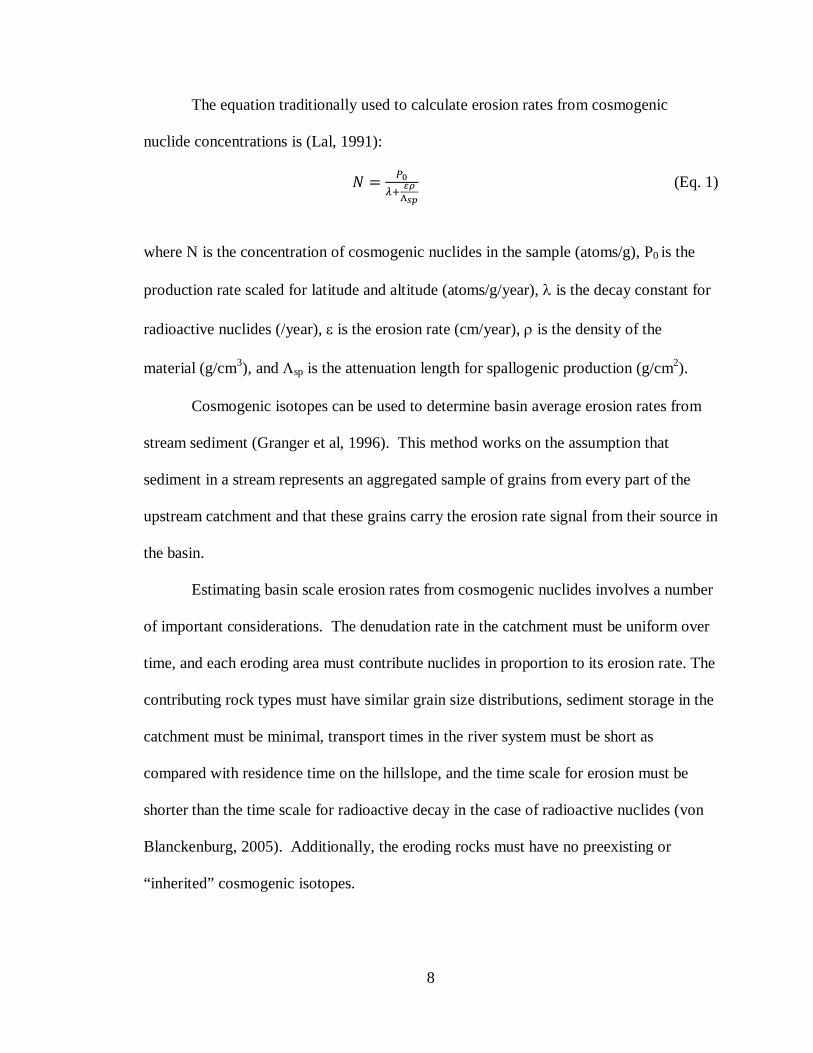
The equation traditionally used to calculate erosion rates from cosmogenic
nuclide concentrations is (Lal, 1991):
𝑁 = 𝑃0𝜆+ 𝜀𝜌
Λ𝑠𝑝
(Eq. 1)
where N is the concentration of cosmogenic nuclides in the sample (atoms/g), P0 is the
production rate scaled for latitude and altitude (atoms/g/year), λ is the decay constant for
radioactive nuclides (/year), ε is the erosion rate (cm/year), ρ is the density of the
material (g/cm3), and Λsp is the attenuation length for spallogenic production (g/cm2).
Cosmogenic isotopes can be used to determine basin average erosion rates from
stream sediment (Granger et al, 1996). This method works on the assumption that
sediment in a stream represents an aggregated sample of grains from every part of the
upstream catchment and that these grains carry the erosion rate signal from their source in
the basin.
Estimating basin scale erosion rates from cosmogenic nuclides involves a number
of important considerations. The denudation rate in the catchment must be uniform over
time, and each eroding area must contribute nuclides in proportion to its erosion rate. The
contributing rock types must have similar grain size distributions, sediment storage in the
catchment must be minimal, transport times in the river system must be short as
compared with residence time on the hillslope, and the time scale for erosion must be
shorter than the time scale for radioactive decay in the case of radioactive nuclides (von
Blanckenburg, 2005). Additionally, the eroding rocks must have no preexisting or
“inherited” cosmogenic isotopes.

9
Estimating paleo-erosion rates from 10Be concentrations measured in ancient
sediments requires several additional assumptions. First, it is assumed that after burial,
the rocks were never reexposed to cosmogenic radiation. If they were, isotopes produced
during the original episode of erosion would be difficult to separate from those produced
in the secondary episode of exposure. Second, the samples must be taken from a
sedimentary sequence with an independently determined chronology so that post-
depositional radioactive decay can be properly accounted for.
Previous Work with Basin Scale Erosion Rates
In the past several decades, cosmogenic nuclides, particularly 10Be, have played
an increasingly important role in determining erosion rates at both outcrop and basin
scales (e.g. Bierman, 1994). In a recent review study, Portenga and Bierman considered
cosmogenically estimated erosion rates from 1599 samples from 87 sites around the
world and found that on a global scale, basin slope yields the strongest correlation with
erosion rates (Portenga and Bierman, 2011).
In the central Andes, Safran et al. (2005) and Bookhagen and Strecker (2012)
have both used 10Be to estimate modern basin-scale erosion rates. In the Cordillera
Oriental and Subandes in Bolivia, Safran et al. (2005) found a strong correlation between
basin-averaged erosion rates and normalized channel steepness index. The normalized
channel steepness index (ks) is a measure of relative gradient, defined as:
S = ksA-θ (Eq. 2)

10
where S is the local channel gradient, A is the basin area, and θ is the concavity index.
Safran et al. (2005) interpreted their data to suggest that tectonically induced patterns of
channel steepness exert the main control on basin scale erosion rates. They also asserted
that precipitation patterns appear to exert no control on basin-scale erosion rates and thus
discard climate as an important forcing mechanism in this region.
In contrast, Bookhagen and Strecker (2012) found a strong correlation between
specific stream power and basin scale erosion rates in the Cordillera Oriental in
northwestern Argentina, which they attribute to precipitation patterns. Bookhagen and
Strecker (2012) emphasize the influence of discharge on specific stream power, and
interpret their data to suggest that discharge (i.e. climate) is an important erosional
forcing factor in this environment. They additionally found a 10-fold increase in erosion
rates along an east-west transect through the South Central Andes, which they relate to
the pronounced regional climatic gradient from dry to wet along the transect.
Safran et al. (2005) and Bookhagen and Strecker (2012)’s interpretations suggest
that tectonic channel steepening and spatial climate variation may both exert controls on
millennial scale erosion rates in the central Andes depending on the dominant local
forcing mechanism. To understand changing erosion rate forcing mechanisms over
longer (million year) time spans erosion rates estimates from older sedimentary rocks
deposited in fluvial systems must be used.
In 2011, Charreau et al. published the first study using cosmogenic 10Be to
estimate erosion rates from ancient fluvial deposits. Working in the Kuitun river
watershed in the northern Tianshan range in China, Charreau et al. estimated erosion
rates over the last 9 Ma and found a significant increase between 2.5 and 1.7 Ma, which

11
they interpret to support Zhang et al. (2001)’s hypothesis that global erosion rates
increased around that time. In their specific area, they attribute the increased erosion to a
shift from a fluvial system to a more erosive glacial system. An important challenge for
Charreau et al. was calculating the scaling factors for production rates in the paleo-Kuitun
watershed. Charreau et al. used an SRTM DEM (Shuttle Radar Topography Mission
Digital Elevation Model) in combination with a geologic map to determine the
production rate for each quartz source. A critical assumption in these calculations is that
the modern watershed is the same size, shape, and elevation as the paleo-watershed from
which the deposited sediments eroded. Charreau et al. were also forced to account for
10Be produced during sediment deposition, which they estimated based on sedimentation
rates using Eq 9.
Zircon Geochronometry and Provenance Studies
Zircons have been successfully used both to determine ages of tuffs (e.g.
Bindemann et al., 2001) and to track sedimentary provenance (e.g. DeCelles et al., 2007).
In this study, we use zircon derived tuff ages to improve the age model for the Río Iruya
section and detrital zircon signatures to monitor changes in the watershed during its
deposition.
Zircon is a zirconium silicate mineral that is extremely resistant to weathering, is
common in felsic and intermediate rocks, and has the useful property of incorporating U
into and excluding Pb from its structure. U has two radioactive isotopes: 238U and 235U,
which decay to 206Pb and 207Pb, respectively (Figure 3). Because the decay rate of each
of the U isotopes is known, the measured ratios of 238U/206Pb and 235U/207Pb can be used
to find the age of formation of the zircon crystal. In practice, the 235U/207Pb ratio is

12
calculated from the 207Pb/206Pb ratio based on a known ratio of 235U/238U in the Earth’s
crust. Comparing the 238U/206Pb and 207Pb/206Pb derived ages using a Concordia diagram
allows us to ensure that the isotope ratios in the zircon crystal have not been altered since
its formation. For young zircons (<1200 Ma), the 238U/206Pb age is more reliable, and
thus is preferred (Gehrels et al., 2012).
Detrital zircon provenance studies use age distributions of zircons from sediment
to determine the provenance of the sediment (Fedo et al., 2003). The general idea is that
different parent materials with different ages contribute to the sediment, and therefore the
ages of the zircons in the sediment can be used to trace the sedimentary provenance. In
order to ensure with 95% confidence that all contributing zircon populations that make up
more than 5% of the total population are sampled, at least 117 grains must be analyzed
(Vermeesch, 2004).
Figure 3. Decay of 238U to 206Pb. 235U decays to 207Pb by a different decay path. (Gehrels, 2012)

13
3. Study Area
Tectonic Setting of the Modern Río Iruya Watershed
The modern Río Iruya watershed encompasses areas of both the Subandean thin-
skinned fold and thrust belt and the Eastern Cordillera in northwestern Argentina making
the Neogene tectonic history of these provinces and the neighboring Puna plateau most
relevant this to this study (Figure 1). The Puna is the internally drained, high altitude
plateau separating the two Cordilleras. The Eastern Cordillera is a high range of
compressionally uplifted sedimentary and metasedimentary rocks, and the Subandes are a
thin-skinned fold and thrust belt that overthrusts the South American Craton (Figure 1).
Gubbels et al. (1993) propose that prior to 10 Ma, the Cordillera Oriental
accommodated most of the crustal shortening, whereas after 10 Ma, the shortening
migrated eastward into the foreland basin, creating the Subandean fold and thrust belt.
Gubbels et al. argue that major compressional deformation in the Cordillera Oriental
ceased after 10 Ma, when significant deformation in the Subandean fold and thrust belt
began (Gubbels et al., 1993).
As compression moved eastward into the shallow foreland basin, the Cordillera
Oriental operated like a bulldozer, thrusting over and down-flexing the Brazilian shield,
and creating a series of N-S striking thrusts (Gubbels et al., 1993). The main detachment
level of these thrusts occurs in Silurian shales and dips 2-3° W (Figure 4). The remainder
of the east verging faults detach from that level (Echavarria et al., 2003). These thin-
skinned thrusts are topographically manifested as N-NE S-SW trending ranges and do not
always break the surface, instead pushing up anticlines. Studies of Neogene foreland
deposits (e.g. Hernández et al., 1996) have led Echavarria et al. (2003) to place the

14
beginning of in-sequence thrusting in the Subandes between 8.5 and 9 Ma at the Cinco
Picachos backthrust. The modern Río Iruya watershed encompasses the Cinco Picachos
backthrust and the El Pescado thrust fault, which was likely reactivated at 4.5 Ma
(Echavarria et al., 2003) (Figure 5). This out of sequence reactivation of the El Pescado
fault ca. 4.5 Ma began uplifting middle and upper Miocene sediments and created the El
Pescado range ca. 2.2 Ma (Figure 4). It is worth noting that Echavarria et al.’s
interpretation of the timing of Pescado Range uplift is based on Hernandez et al. (1996)’s
suggestion that sedimentary provenance in the Río Iruya section changed from the
Eastern Cordillera to the El Pescado Range at that time. If, with uplift of the El Pescado
range, the Río Iruya watershed temporarily lost contact with the Cordillera Oriental, the
average elevation of the watershed would be much lower than the modern watershed,
requiring a lower elevation scaling factor for 10Be production rates. Additionally, if the
sediment deposited in the Río Iruya after the El Pescado reactivation was eroded from the
middle and upper Miocene sediments of the El Pescado range, it may carry an inherited
10Be signal from the original erosion and deposition of those sediments.

15
Bedrock Geology of the Modern Río Iruya Watershed
The modern Río Iruya watershed encompasses Proterozoic, Cambrian, and
Ordovician bedrock lithologies in the Cordillera Oriental (Figure 5). The metamorphic
Proterozoic basement of the Cordillera Oriental in this region is made up of greenschists,
slates, phyllites, and metagraywackes. Also underlying the watershed, although with
much lower areal distribution, are Cambrian facies of silicified sandstones, with some
mudstones. Finally, a large area of the watershed overlies lower Ordovician siltstones,
mudstones, and fine-grained sandstones .
The areally much less significant portion of the watershed in the Subandes
includes formations from the Silurian through the Miocene. The Silurian formations
include siltstones and claystones. The Devonian formations are made up of fine to
medium grained sandstones and silicified conglomeratic sandstones. The Carboniferous
Figure 4. Structural growth model for the Subandean fold and thrust belt. The Río Iruya section is labeled to the east of the El Pescado Range at 4.5 and 2 Ma. (Echavarria et al., 2003)

16
Figure 5. Bedrock geology of the modern Río Iruya watershed. The modern Río Iruya watershed is outlined in blue. Figure modified from the La Quiaca and Ciudad del Libertador San Martín geologic maps (SEGEMAR, 2012).

17
sediments include sandstones and diamicton with interbedded mudstones and
conglomerates. Finally, the Miocene formations are composed of mudstones, claystones,
silty sandstones, and polymictic conglomerates. The formations in the Subandean section
of the watershed occur primarily in a large syncline bordered by the Cinco Picachos and
the Pescado Ranges (Figure 5) (La Quiaca, Ciudad de Libertador General San Martin
Geologic Maps, 2012).
Climatic Setting of the Subandes and Cordillera Oriental
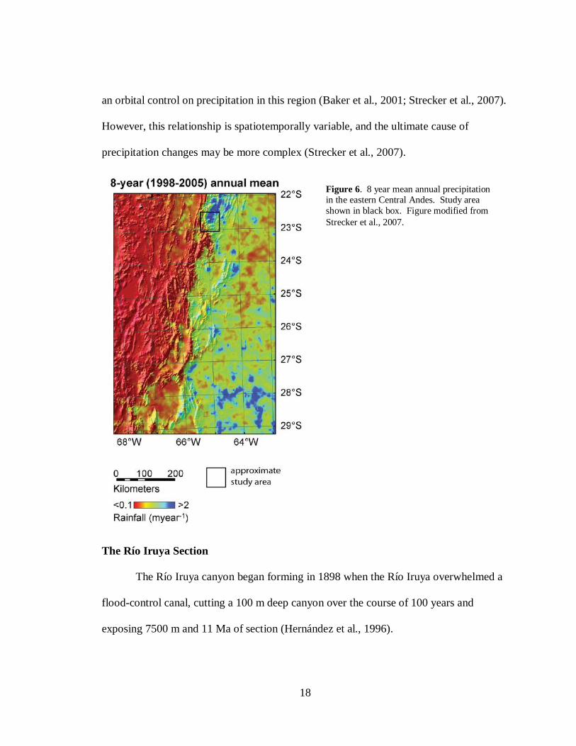
The modern Cordillera Oriental and Subandean belt receive between 1 and 3 m of
precipitation annually (Strecker et al., 2007) (Figure 6). In the area of this study, the high
elevation headwaters receive less than 0.1 m of annual precipitation whereas lower
elevations receive over 1 m. 80% of this precipitation falls during the austral summer,
between November and February. During summer, east moving, moisture-laden air from
the Amazon is forced south, and upon encountering the orographic barrier of the Andes,
drops precipitation on the Subandes and Cordillera Oriental (Garreaud et al., 2008).
These annual convective rainfall cycles are interpreted to have begun at approximately
10.3 Ma when the Andes rose to sufficient heights to create an effective orographic
barrier (Poulsen et al., 2010).
There have been changes in the amount of precipitation in this area over time.
For example, during the last glacial maximum (LGM), precipitation apparently increased
along the eastern flank of the Andes, in contrast with a global increase in aridity (Cook
and Vizy 2006). These increases in precipitation have been correlated with increases in
summer insolation maxima on the Puna/Altiplano plateau, suggesting that there may be
18
an orbital control on precipitation in this region (Baker et al., 2001; Strecker et al., 2007).
However, this relationship is spatiotemporally variable, and the ultimate cause of
precipitation changes may be more complex (Strecker et al., 2007).
The Río Iruya Section
The Río Iruya canyon began forming in 1898 when the Río Iruya overwhelmed a
flood-control canal, cutting a 100 m deep canyon over the course of 100 years and
exposing 7500 m and 11 Ma of section (Hernández et al., 1996).
Figure 6. 8 year mean annual precipitation in the eastern Central Andes. Study area shown in black box. Figure modified from Strecker et al., 2007.

19
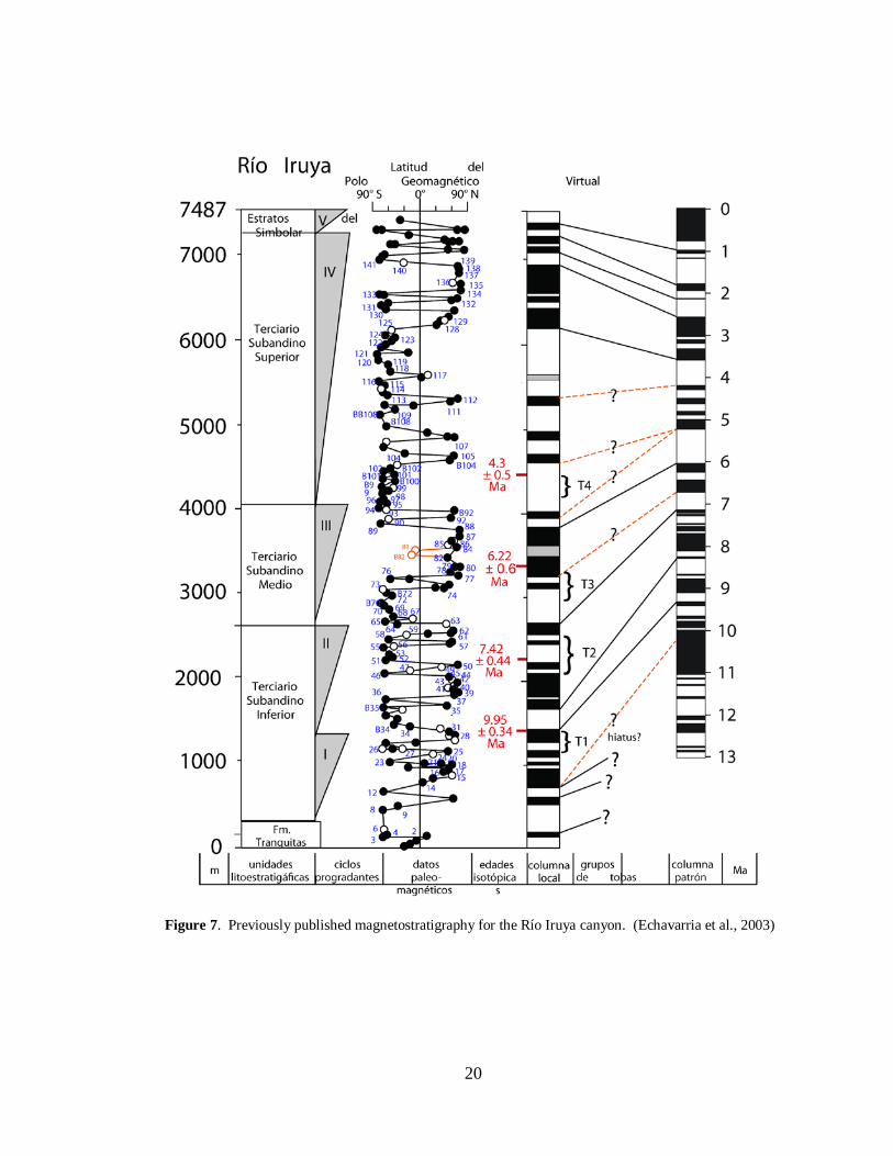
In a comprehensive stratigraphic study of the canyon, Hernández et al. (1996)
collected 196 samples for paleomagnetic dating. In addition, they obtained two zircon
fission track dates for ashes preserved in the section. Echavarria et al. (2003) provide
two additional ash dates and a new interpretation of the magnetostratigraphy (Figure 7).
In general, Echavarria et al.’s magnetostratigraphy column is poorly resolved with the
magnetic polarity reference scale, and the interpretation leaves some questions.
In their stratigraphy, Hernández et al. (1996) identify three major progradational
cycles in the Río Iruya section, which are collectively known as the “Terciario
Subandino.” Facies within these cycles have been interpreted as alluvial fan, braided
stream, distal ephemeral fan, and mud flat deposits (Hernández et al., 1996). This study
targets the sediments in the canyon that were deposited between approximately 3.4 and 1
Ma (Figure 8) and make up part of the third progradational cycle and the overlying
sedimentary deposit known as El Simbolar. Hernández et al. argue that the sediments of
the third progradational cycle came from the Pescado Range and that the El Simbolar
strata are conglomerate beds that were deposited after the Río Iruya and Río Pescado (a
major tributary) cut through the Pescado Range, bringing sediment from the Cordillera
Oriental once more with a heightened sedimentation rate of 1 mm/yr. Sediments at the
base of the third cycle, which Hernández et al. place at 5.7 Ma, are characteristic of
alluvial fan sediments, which they interpret to have been deposited at the base of the
Pescado Range at a rate of 0.8 mm/yr. It is worth noting that this age does not agree with
Echavarria et al.’s interpretation of uplift on the El Pescado thrust, suggesting that better
age control is needed. Above these are facies that correspond to growth strata, alluvial
20
Figure 7. Previously published magnetostratigraphy for the Río Iruya canyon. (Echavarria et al., 2003)

21
Figure 8. Sampling locations for cosmogenic 10Be, detrital zircon, and ash samples in the Río Iruya canyon. Gray dashed lines are drawn along strike and represent the age of the bed at that location.

22
fans, and braided rivers, with sedimentation rates that begin to taper off at approximately
2.5 Ma (Hernández et al., 1996).
The sediments of this study are exposed in the upper section of the Río Iruya
canyon and are dominantly conglomerates with some interbeds of mudstones and
sandstones. The conglomerate beds contain 1 – 15 cm clasts in a medium to coarse-
grained sand matrix and represent a braided river environment similar to the modern
environment (Hernández et al, 1996). The interbeds of red mudstones correspond to mud
flats formed during flooding events (Hernández et al., 1996).
23
CHAPTER II
1. Field Methods
Sediment Collection for Cosmogenic 10Be and Ash Collection for Zircon Dates
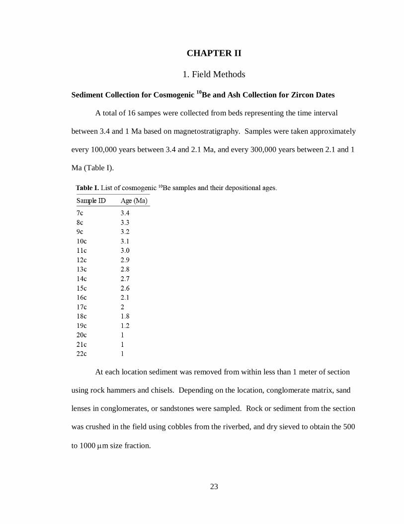
A total of 16 sampes were collected from beds representing the time interval
between 3.4 and 1 Ma based on magnetostratigraphy. Samples were taken approximately
every 100,000 years between 3.4 and 2.1 Ma, and every 300,000 years between 2.1 and 1
Ma (Table I).
At each location sediment was removed from within less than 1 meter of section
using rock hammers and chisels. Depending on the location, conglomerate matrix, sand
lenses in conglomerates, or sandstones were sampled. Rock or sediment from the section
was crushed in the field using cobbles from the riverbed, and dry sieved to obtain the 500
to 1000 µm size fraction.

24
Five ash layers were found interbedded with the sandstones in this section. Ashes
were removed with rock hammers and stored in cloth bags.
2. Laboratory Methods
Quartz Purification
The quartz purification process used in this study is modified from the processes
used in Paul Bierman and Bodo Bookhagen’s labs at the University of Vermont and the
University of California-Santa Barbara, respectively. These protocols are available
online at
http://www.uvm.edu/cosmolab/?Page=methods.html&SM=methods_sub_menu.html and
http://www.geog.ucsb.edu/~bodo/pdf/bookhagen_chemSeparation_UCSB.pdf .
The first step in the quartz purification process was to clean and re-sieve the field
sieved 500-1000 µm sediment fraction. The sediment collected in the field was
frequently coated in very fine- grained silts and clays and was sometimes aggregated.
Once these fine-grained sediments were removed, much of the quartz fell into the 300-
500 µm size fraction, so the sand was wet-sieved using a 300 µm sieve until the water
passing through the sieve ran clear. This served to both capture only the 300-1000 µm
size fraction and to wash away extraneous fine sediment.
The second step was to magnetically isolate non-magnetic quartz from other
magnetic sediment using a Frantz isodynamic separator. Two passes were performed on
the sediment, one at 1.0 A and one at 1.8 A, with each pass removing approximately half
of the sediment present.
25
The non-magnetic fraction was then sonicated for at least 12 hours in 6N HCl in
an ultrasonic bath to remove any remaining clay as well as oxide coats and meteoric 10Be
from the grains. 120 g of sediment was added to 1 L of 6N HCl. After sonicating, the
acid was poured off into a waste container and the sediment rinsed well using deionized
water and dried at about 50°C.
After drying, quartz was separated from the HCl treated sediment using lithium
polytungstate (LST). The sediment was suspended in LST, which has a density of 2.95
g/mL at 25°C. Water was mixed with the LST to reduce the density of the liquid until the
majority of the quartz was floating. The heavy minerals were then removed and the
remaining sediment was rinsed clean of LST.
The samples were then etched in a 1% HF and 1% HNO3 solution. Samples went
through three at least 18 hour etches in either an ultrasonic bath or on a commercial hot
dog roller with at least two of the three etch cycles occurring in an ultrasonic bath.
Samples 7c-13c were determined to be impure after 3 etches and were etched once more
for 24 hours in an ultrasonic bath. For the first etch cycle, 30 grams of sample were
added to 4L of dilute HF/HNO3 mixture. For the second and third etches, approximately
50 g of sample were added to 4L of dilute acid mixture. Between etches, the samples
were rinsed well with deionized water. After three etching cycles, samples were dried at
approximately 50°C and set aside for purity testing.
Quartz Purity Testing
To test the quartz for purity, between 0.15 and 0.25 g of quartz was weighed into
clean Teflon vials. Five mL of 2:1 concentrated HF/HNO3 mixture and .05 mL

26
concentrated H2SO4 were added to each vial. Each vial was covered with a Teflon watch
glass and heated for 6 hours at a temperature just below the boiling point of the acid
mixture. After 6 hours, the watch glasses were removed and the HF/HNO3 mixture
allowed to evaporate, leaving a small bead of H2SO4 with the dissolved quartz. Once the
HF/HNO3 mixture had evaporated, 2 mL of concentrated HNO3 was added to the vials,
and they were capped and shaken vigorously to mix in the H2SO4 and quartz solution.
This HNO3 solution was then added to approximately 25 mL of milli-q purified water in
a pre-weighed bottle. The bottles were capped and shaken vigorously to mix in the
HNO3 and quartz solution.
Concentrations of Ti, Al, Fe, Mn, Mg, Ca, Na, and K in this solution were then
measured using an Inductively Coupled Plasma – Atomic Emissions Spectrometer (ICP-
AES) at Middlebury College and used to calculate the concentration of these elements in
the quartz. Pure quartz should have a minimal amount of these elements. The ICP-AES
was standardized using 25 ppm Spex Solution diluted to 1 and 5 ppm and a blank
solution of 5% HNO3.
Beryllium Extraction Chemistry
Beryllium was extracted from the cleaned quartz samples following the methods
outlined in Bookhagen and Strecker, 2012. A detailed methodology is available at
http://www.geog.ucsb.edu/~bodo/pdf/bookhagen_chemSeparation_UCSB.pdf. Burch
Fisher performed the Be extraction chemistry at UCSB during December, 2012 and
January, 2013.
27
Our clean quartz samples weighed between 96 and 381g, depending roughly on
their age. Younger samples required less quartz because the beryllium present has had
less time to decay, and thus the overall concentration is higher than in older samples.
These clean samples were dissolved in concentrated HF and a low 10Be/9Be spike was
added. AMS measurements are reported in terms of 10Be/9Be ratios, so the idea behind
adding a 9Be spike is to swamp any naturally occurring 9Be in the sample. Then, because
we know the amount of 9Be added, we can easily calculate the concentration of 10Be in
our sample from the measured ratio.
After dissolution, Be and Al were separated from the samples by ion exchange
chromatography. The quartz solution was added to resin columns, which preferentially
hold different cations at different pHs. By carefully adjusting the pH of the column using
oxalic and hydrochloric acid, Be can be eluted at a specific step, allowing for full
recovery of the Be in the sample.
The Be eluted from the column was then converted to Be(OH)2 and ignited to
form BeO, the required compound for AMS measurements. This solid was ground up
with Niobium in a glove box and packed into targets for analysis by AMS.
Measuring 10Be with AMS
Atomic mass spectrometry measurements were done at the Purdue Rare Isotope
Measurement (PRIME) Laboratory at Purdue University. When the 10Be sample is
loaded into the AMS, atoms are sputtered from the surface of the solid and concentrated
into an ion beam in the ion source. This beam is then fed into the injector magnet, which
performs an initial separation of ions based on atomic mass. The separated ions then
28
flow into the tandem accelerator, which accelerates the ions to velocities that are within a
few percent of the speed of light. These ions then pass through the analyzing and
switching magnets, which select the isotope of interest, and send it along to the
electrostatic analyzer and gas ionization detector. The electrostatic analyzer selects
particles based on their energy, and the gas ionization detector counts the individual ions
as they arrive, additionally checking which isotope it is to ensure that the count is correct.
Isotope ratios are measured by alternately selecting for 10Be and 9Be using the injector
and analyzer magnets during the analysis
(http://www.physics.purdue.edu/primelab/introduction/ams.html).
Ash Zircon Separation
Zircon separation was performed at Middlebury College during January, 2013.
Zircon was separated from 5 ash layers found interbedded in the Río Iruya section for U-
Pb dating. The procedure used generally follows the methods described in “A Guide to
Mineral Separation” (Amidon, 2010).
Tephra was sampled in the field using rock hammers and returned to Middlebury
College as pieces of rock. The rock was then crushed using the chipmunk and disc mill
and sieved for the <250 µm size fraction. The <250 µm size fraction was then rinsed,
sonicated in 1% HF/HNO3 solution for approximately 1 hour with occasional vigorous
stirring, and then rinsed thoroughly in a large plastic container until the water used for
rinsing ran clear. Special care was taken during the rinsing steps to allow the sediment to
settle for at least 30 seconds before pouring off the water in order to avoid washing away
zircons. The remaining sediment was then dried at approximately 65°C.

29
After drying, the non-magnetic fraction was separated from the rest of the ash
using a Frantz Isodynamic Magnetic Separator. Zircon was then separated from the non-
magnetic fraction in methylene iodide (MEI, density = 3.3 g/mL) using a separatory
funnel. The zircon was rinsed thoroughly with acetone and dried under a heat lamp.
The zircon grains were then mounted in 1-inch diameter epoxy discs using
Araldyte epoxy. The mounts were polished using 1µm silica solution on an autopolisher
until the center of the grains were exposed on the largest possible number of zircons.
Detrital Zircon Separation
Detrital zircon separation was performed at Middlebury College from September,
2012, to January, 2013, following the methods described in “A Guide to Mineral
Separation” (Amidon, 2010). Zircon was separated from 2 modern detrital samples from
the Río Iruya catchment and 4 paleo-detrital samples from the Río Iruya section. The
methods closely parallel those described above for ash zircons, with a few slight
differences.
The sediment was collected from the same sedimentary rocks that the cosmogenic
10Be samples came from, and was sieved in the field to <500 µm. Once in the lab, the
samples were dry sieved for the <210 µm fraction. They were then treated like the ash
zircon samples, but were not sonicated in HF/HNO3. After heavy liquids separation, the
heavy fraction was not pure zircon in some of the samples. The heavy fraction in these
samples was subjected to a round of heated etching in concentrated HF/HNO3 solution to
dissolve away the non-zircon minerals.

30
Cathodoluminescence Imaging
Cathodoluminescence (CL) imaging was performed on the ash-separated zircons
using the cathodoluminoscope at Rensselaer Polytechnic Institute to reveal mineral
characteristics that are not visible in reflected or transmitted light, such as internal zoning
patterns and inherited core boundaries and to provide context for placing laser ablation
points
The cathodoluminoscope works by magnetically directing a beam of X-rays from
the cathode ray source across a sample and causing it to emit visible light, which is then
observed through a standard microscope. We attempted to optimize the images by
magnetically manipulating the beam to produce the brightest and most informative
images possible (Figure 9).
Figure 9. Cathodoluminescence image of zircons from Ash 5. Note the zoning in the uppermost zircon.

31
U-Pb Dating with LA-MC-ICPMS
We dated zircons from 5 ash layers interbedded in the Río Iruya canyon, 2 detrital
zircon samples from the modern Río Iruya catchment (Figure 10), and 4 paleo-detrital
zircon companion samples to cosmogenic samples from the Río Iruya canyon (Figure 8).
U-Pb dating of zircon was carried out using laser ablation multi collector inductively
coupled plasma mass spectrometry (LA-MC-ICPMS) at UCSB in February 2013.
Detailed methodology and laboratory information can be found in Kylander-Clark et al.,
2013.
Figure 10. Sampling locations of modern detrital zircon samples.
32
The UCSB LASS facility features a Nu Plasma HR MC-ICPMS (Nu Instruments
Ltd., Wrexham, UK) coupled with an Analyte 193 ARF Laser Ablation system (Photon
Machines, San Diego, USA), which were used in this analysis. LA-ICPMS delivers
quick and precise isotope measurements from zircon, allowing many grains to be
measured over a relatively short period of time (Gehrels, 2008). LA-ICPMS therefore
lends itself particularly well to detrital zircon studies, where many grains must be
measured to significantly characterize a population (Vermeesch, 2004). In LA-ICPMS,
the laser ablates sample from the surface of a polished crystal. The resulting aerosol is
carried from the sample chamber and into the ICPMS, where it is ionized and accelerated
toward the magnetic field. The magnetic field then separates the isotopes based on mass
and feeds them into the collectors where they are measured by Faraday cup or low mass
ion counter (Gehrels, 2008).
For the ash samples, spot locations for laser ablation were chosen in
conjunction with previously produced CL images and reflected light microscopy.
Metamict grains, xenocrystic core boundaries, and cracks or pits in individual grains were
avoided. We dated approximately 40 grains per sample.
Polished samples mounted in 1in diameter Araldyte epoxy discs were loaded into
the sample chamber. Each spot on every individual grain was initially subjected to two
cleaning shots from the laser to remove any surficial contamination. For the ash zircons,
we used a 30 µm diameter laser spot and ablated for 80 counts at a repetition rate of 4 Hz
and an energy of 3 mJ and 65%. Standard zircon crystals 91500 (Wiedenbeck et al.,
1995, Kylander-Clark et al., 2013) and GJ1 (Jackson et al., 2004, Kylander-Clark et al.,

33
2013) were sampled at the beginning of the run, every 8 samples during the run, and at
the end of the run.
For the detrital zircon samples, laser spots were selected using reflected light
microscopy without reference CL images, and were scattered over many different grains
in an attempt to minimize sampling bias and achieve representative age distributions
while avoiding metamict grains and cracked or pitted regions in individual grains. We
dated approximately 150 grains per sample using a 15 µm laser spot at 65 counts. All
other parameters were the same as for the ash zircons.
3. Analytical Methods
Tuff Age Determination from Single Grain LA-ICPMS 238U/206Pb and 207Pb/206
Dates
Ages were computed for individual grains using measured 238U/206Pb and
207Pb/206Pb ratios. For grains younger than 1200 Ma, the reported age is the 238U/206Pb
age. In order to determine the age of the tuff from our collection of single grain dates, we
first rejected all analyses that were more than 10% discordant. For the remaining dates,
we used the TuffZirc function in Isoplot to find the age of the tuff based on the youngest
coherent cluster of single-grain dates (Ludwig and Mundil, 2002). The reported Tuffzirc
age is the median age of the cluster with 95% confidence errors of the median age as its
uncertainty (Ludwig, 2012).

34
Detrital Zircon Ages and Kernel Density Estimation Plots
Detrital zircon ages were also computed from measured 238U/206Pb and 207Pb/206Pb
ratios. For grains younger than 1200 Ma, 238U/206Pb ages are reported as the age of the
grain. For grains older than 1200 Ma, the 207Pb/206Pb age is given. In order to compare
detrital zircon age distributions between samples, we rejected ages that were more than
5% discordant and used the remaining ages to create kernel density estimation plots
(KDEs). A KDE is an estimate of the probability density function of the population from
which the sample was drawn, which reflects the relative likelihood of different ages
occurring in the population (Vermeesch, 2012). KDEs were generated from reported ages
using DensityPlotter, a Java based computer program that is available online at
http://densityplotter.london-geochron.com (Vermeesch, 2012).
Erosion Rate Determination from 10Be Concentration
To calculate erosion rates from measured 10Be concentrations, we first correct for
10Be decay since the time of deposition, subtract 10Be that accumulated during deposition,
calculate a basin averaged production rate, and then estimate an erosion rate. The
MATLAB code used to do these calculations is available in Appendix C.
The equation used to calculate a basin averaged erosion rate is (Bierman, 1994):
Ε = Λ𝜌�𝑃𝑎𝑣𝑔𝑁𝑒
− 𝜆� (Eq. 3)
where: E = basin averaged erosion rate (cm/year) Λ = attenuation length (165 g/cm2) ρ = density of rock (2.7 g/cm3) Pavg = basin averaged production rate (atoms/g*year) Ne = concentration of 10Be in quartz at the time of deposition (atoms/g) λ = 10Be decay constant (5.1 x 10⁻⁷ /year)
35
To find P, the basin averaged production rate, we scaled the sea-level, high
latitude (SLHL) production rate of 4.7 atoms/g*year (Balco et al., 2009) for latitude
according to Lal (1991) using Cosmocalc (Vermeesch, 2007), and for atmospheric depth
following Stone (2000):
𝑃 = 𝑆𝐿𝐻𝐿 ∗ 𝑆𝐹 ∗ 𝑒(1037−𝑑)
Λ (Eq. 4)
where: P = production rate (atoms/g*year) SLHL = Sea-level, high-latitude spallogenic production rate (4.7 atoms/g*year) SF = Lal scaling factor based on latitude d = atmospheric depth (g/cm2) Λ = attenuation length (g/cm2)
We calculated the production rate for every pixel in a 30m ASTER GDEM digital
elevation model of the modern Rio Iruya watershed, and took the average of these values.
This is Pavg, the basin averaged production rate.
The initial concentration of 10Be in quartz at the time of deposition (Ni) is given
by Eq. 5 (Balco, 2006):
𝑁10 = 1𝑀𝑞�𝑅10/9𝑀𝐶𝑁𝐴
𝐴𝐵𝑒− 𝑛10.𝐵� (Eq. 5)
where: N10 = Concentration of 10Be in quartz sample (atoms/g) Mq = Mass of original quartz sample (g) R10/9 = Ratio of 10Be/9Be from AMS Mc = Mass of 9Be spike added to sample (g) NA = Avogadro’s number (6.022 x 10²³ atoms/mol) ABe = Molar mass of Be (9.012 g/mol) n10.B = 10Be concentration in the process blank (atoms/g)
The concentration of 10Be in the quartz must then be corrected for radioactive
decay and cosmogenic nuclide accumulation since the time of deposition. To correct for
36
radioactive decay, we must know the decay constant of 10Be and the time of deposition of
the sample. The equation used to correct for radioactive decay is:
𝑁𝑖 = 𝑁10𝑒−𝜆𝑡
(Eq. 6)
where: Ni = Initial decay corrected 10Be concentration in quartz (atoms/g) N10 = Concentration of 10Be in quartz sample (atoms/g) λ = 10Be decay constant (5.1x10⁻⁷ /year) t = Age of sample (year)
The concentration Ni is a combination of the 10Be that accumulated during erosion
(Ne) and the 10Be that accumulated during burial (Nb), such that:
𝑁𝑖 = 𝑁𝑒 + 𝑁𝑏 (Eq. 7)
And solving for Ne:
𝑁𝑒 = 𝑁𝑖 − 𝑁𝑏 (Eq. 8)
Where: Ne = 10Be concentration accumulated during erosion (atoms/g) Ni = Initial decay corrected 10Be concentration in quartz (atoms/g) Nb = 10Be concentration accumulated during burial (atoms/g)
To find the concentration of 10Be accumulated during burial, we need to know the
rate of accumulation, the production rate at the site of deposition, the density of the
sediment, the decay constant of the cosmogenic nuclide, and the attenuation length. Then
we can calculate Nb:
𝑁𝑏 = 𝑃
𝜆−𝐴𝑟𝜌Λ∙ �𝑒
−𝑇𝐴𝑟𝜌Λ − 𝑒−𝜆𝑇� (Eq. 9)

37
Where: Nb = 10Be concentration accumulated during burial (atoms/g) P = 10Be production rate scaled for latitude and atmospheric depth (atoms/g*year) λ = Decay rate of 10Be (5.1x10⁻⁷ /year) Ar = Accumulation rate (m/year) ρ = Density of sediment (2.4 g/cm3) Λ = Attenuation length (165 g/cm2) T = time to bury to 3 m depth (years) = (3m/Ar)
We used accumulation rates for the Rio Iruya section that were previously
published in Echavarria et al. (2003) (Figure 11).
By solving Eq. 8 for Ne, we get the 10Be concentration that accumulated during erosion or
the concentration of 10Be in quartz at the time of deposition. We then have all the
necessary elements to estimate the erosion rate in the Rio Iruya catchment at the time that
the sample was deposited using Eq. 3.
Figure 11. Sediment accumulation rates for the Río Iruya canyon section (Echavarria et al., 2003).

38
CHAPTER III
1. Results
Ash Zircon Ages
Of the five ashes from which we dated zircons, only the oldest three produced
significant clusters of young ages interpretable as the time of ash emplacement (Table II).
Ash 5 is 7.01 +0.10/-0.04 million years old, which is several hundred thousand years
older than Hernandez et al. (1996)’s magnetostratigraphy age for that part of the section.
Ash 4 has an age of 4.07 +0.07/-0.03 Ma, which is younger than the magnetostratigraphy
age, and Ash 1 has an age of 2.77 +0.05/-0.06 Ma, which agrees well with the
magnetostratigraphy ages. In contrast, the youngest age from Ash 2 is 341 Ma, and the
youngest age from Ash 3, is 4.9 Ma. 4.9 Ma is still too old to be the eruption age of the
ash because the ash is stratigraphically much younger than Ash 1, which had a reliable
cluster of ages around 2.77 Ma.

39
Detrital Zircon Age Distributions
Kernel density estimation plots for each detrital zircon sample are presented in
Figure 12. Sample 3M is from the main stem of the modern Río Iruya upstream of Isla
de Cañas and is representative of the modern watershed above that point (Figure 10).
Sample 4M is from the Río Nazareno just upstream of the confluence with the Río Iruya.
Samples 15N, 27C, 5C, and 22C are all paleo-detrital samples from the Río Iruya canyon
sedimentary section. These samples and their magnetostratigraphy ages are summarized
in Table III.
For the purposes of qualitative comparison between the samples, the most
diagnostic peaks in the KDEs have been assigned as follows: A: 50-210 Ma, B: 200-400
Ma, C: 400-750 Ma, D: 900-1200 Ma, and E: 1400-1550 Ma (Figure 12).

40
Figure 12. Kernel density estimation plots derived from two modern and four paleo-detrital zircon samples. The y-axis represents the probability of an age occurring. The circles below the x-axis represent the ages of the zircon grains in each sample.

41
Cosmogenic 10Be Erosion Rate Estimates
Erosion rate estimates for sixteen samples from the Río Iruya section are
presented in Table IV. These preliminary estimates were calculated using the modern
Río Iruya watershed hypsometry for production rate estimation, and assuming that the
sediment was buried rapidly. Post-depositional 10Be production was not accounted for,
but could be once sedimentation rates are better constrained.
42
CHAPTER IV
1. Discussion
Improved Age Model for the Río Iruya Section
We have reinterpreted the previously published field polarity column (Echavarria et
al., 2003) based on the 2004 astronomically tuned polarity reference scale (Lourens et al.,
2004) and our three zircon derived tuff ages (Figure 13). Our samples are correlated with
the field polarity column based on known previous magnetostratigraphy sampling
locations in the canyon (Jim Reynolds, personal communication).
Ash 1, with an age of 2.77 +0.05/-0.06 Ma, falls near the bottom of the C2An chron,
which is well defined in the field polarity column. The tuff age in this case agrees with
the original magnetostratigraphy age.
Ash 4 has an age of 4.07 +0.07/-0.03 Ma, which corresponds to the C2Ar chron of the
polarity reference scale. This age does not agree with the original magnetostratigraphy
age of 4.3 Ma, corresponding to the C3n.1r chron. There are two possible reasons why
the tuff age does not agree with the magnetostratigraphy age. The first possibility is that
the field polarity column is misaligned with the polarity reference scale at that point.
Directly above the ash in the field polarity column, there is a poorly defined normal
period that is interpreted as the C3n.1n chron. If that normal period does not in fact exist,
the normal period directly below the ash could be correlated with the C3n.1n chron
instead, which would realign the column and give a magnetostratigraphy age of 4.1 Ma
for Ash 4. The second possibility is that the tuff age is wrong. The three zircons dates
defining the tuff age are not perfectly concordant, meaning that they could have
experienced Pb loss, causing an age underestimation. If the apparent tuff age were wrong

43
Figure 13. Tuff ages from the Río Iruya section and new magnetostratigraphy interpretation. Field polarity column from Echavarria et al., 2003, polarity reference column after Lourens et al., 2004).

44
by only 200,000 years, the original magnetostratigraphy age of 4.3 Ma would agree with
the tuff age. It is more likely that the tuff age is wrong than that the normal period
directly above the tuff did not occur, therefore the normal period above the tuff is
correlated with the C3n.1n chron in the new interpretation.
Zircons from Ash 5 produced an age of 7.01 +0.10/-0.04 Ma, which likely falls
within the C3Ar reverse chron in the polarity reference column. However, the
stratigraphic location of Ash 5 is within a well-defined normal period in the field polarity
column. If the apparent tuff age were too young by only 150,000 years, the normal
period in the field polarity column in which it falls would be well correlated with the
C3Bn period, giving a magnetostratigraphy age of 7.15 Ma for Ash 5. Due to the general
agreement of reversals above the ash with the C3An.1n and C3An.2n chrons, the normal
period within which the ash falls is assigned to the C3Bn chron.
Provenance Changes in the Río Iruya Watershed
Comparing paleo-detrital zircon KDEs with modern detrital zircon signatures and
geologic maps allow us to constrain provenance changes and interpret the evolution of
the watershed over time.
Sample 4M, the modern sample from the Río Nazareno upstream of the
confluence with the Río Iruya, describes a relatively small provenance region containing
predominately Proterozoic basement and Cambrian/Ordovician sedimentary rocks
(Figure 10). The large C peak and smaller D peak present in its signature represent the
relative contributions of each of these units to the detrital zircon signature in this area
(Figure 12). Both the Cambrian/Ordovician sedimentary rocks and the Proterozoic
45
basement produce C and D peaks, but in different proportions. Working close to our
study area, DeCelles et al. found that Ordovician sedimentary rocks similar to those in the
modern Río Iruya watershed display larger C peaks than D peaks (DeCelles et al., 2007).
Adams et al. found that the Puncoviscana Formation that makes up the Proterozoic
basement in this area (shown in salmon in Figure 5) displays larger D peaks than C peaks
in some areas (Adams et al., 2008). The large C to D peak ratio in the Río Nazareno
signature is likely caused by a large areal proportion of Cambrian and Ordovician rocks
to Proterozoic rocks in the watershed.
In contrast, sample 3M, which represents the entire modern watershed including
the Nazareno watershed, has a smaller peak C to D ratio than 4M. The entire watershed
encompasses a greater proportion of Proterozoic rocks than the Nazareno watershed,
which likely increases the peak D size in the 3M signature.
Peaks A and B are present in the paleo-detrital signatures and represent
contributions from formations to the west of the modern watershed. Peak A does not
occur in either of the modern samples and peak B only occurs in sample 3M and is
defined by one grain. This peak absence suggests that the paleo-river sourced material
that it no longer has access to in the modern watershed.
West of the modern watershed, there are several plutons that would produce ages
young enough to fall into peak A, while there is really only one formation that could have
produced ages that would fall into peak B. Potential sources of Peak A zircons include
the granitic Jurassic/Cretaceous Fundición, Tusaquillas, and Aguilar Formations. Peak B
zircons most likely originated in other more distant plutons and were deposited in the
Cretaceous Pirgua Subgroup before being remobilized and deposited in the Río Iruya

46
section. The Pirgua Subgroup occurs in a very small area of the modern watershed, as
shown in green in Figure 5.
The known sources of Peaks A, B, C, and D can now be used to characterize the
paleo-watersheds that the paleo-detrital zircon samples represent. Sample 15N is most
likely greater than 10 million years old, although its exact age is unknown due to a thrust
fault in the section above it. The presence of peak B suggests that the watershed was
sourcing the Pirgua subgroup to the west of the modern drainage divide, but the absence
of peak A indicates that it was not reaching far enough west to incorporate peak A
plutons. The peak C to D ratio is similar to the modern watershed, indicating that the
15N watershed may have incorporated similar areal proportions of the Cambrian-
Ordovician and Proterozoic units to the modern watershed (Figure 14).
Sample 27C was deposited at approximately 6.3 Ma and is similar to 15N,
although it contains one grain in peak A, suggesting that the watershed may have begun
to access the plutons. The spread of ages above 1200 Ma is wider than in 15N, which
suggests that the 27C watershed was sourcing a different area of the basement than the
15N watershed (Figure 14).
Sample 5C is between 3.5 and 3.6 million years old and indicates a dramatic
change in the watershed. The large ratio of peak C to D suggests that the watershed was
sourcing more Cambrian-Ordovician sediments than Proterozoic basement. The
appearance of a strong peak A indicates that the watershed had good access to the
Jurassic-Cretaceous plutons (Figure 14).
Sample 22C is about 1 million years old and indicates another big change. Peaks
A and B disappear, suggesting that the watershed was cut off from the western source

47
Figu
re 1
4. C
hang
es in
the
Río
Iruy
a w
ater
shed
ove
r the
pas
t 10
Ma
base
d on
det
rital
zirc
on in
terp
reta
tions
.

48
area of these zircons. The peak C to D ratio is the smallest of any sample, suggesting that
the watershed was sourcing an even larger proportion of Proterozoic basement rocks than
it is today. Additionally, the distribution of peaks above 1200 Ma is similar to the modern
watershed, suggesting that the watershed was sourcing a similar area of basement rocks
as it is today (Figure 14).
Evolution of the Río Iruya Watershed
Approximately 10 million years ago, the watershed reached farther eastward than
it does now, but not so far east as to incorporate significant contributions from the
Jurassic/Cretaceous plutons. Between 10 Ma and 3.5 Ma, rivers in the watershed eroded
progressively westward into the eastern Cordillera, sourcing greater areas of Cambrian-
Ordovician sediments and gaining access to Jurassic and Cretaceous plutons. This
westward erosion may have been caused by base level lowering as the Subandean fold
and thrust belt propagated out downflexing the foreland basin and providing increased
stream power to rivers in the watershed. Then, sometime between 3.5 and 1 Ma, the
drainage divide migrated significantly eastward, potentially even farther eastward than
where it exists today. This event likely occurred very close to 1 Ma, and is probably
indicated in the field by a significant change in dip and detrital quartz color. A potential
cause of this change would be a significant stream capture event wherein the Río Grande
captured the western portion of the Río Iruya watershed and began carrying that sediment
southward.

49
Implications for Erosion Rate Calculations
In preliminary erosion rate calculations, we have used a basin averaged 10Be
production rate based on the modern watershed; however, the paleo-watershed most
likely incorporated a significantly larger high altitude area than the modern watershed
does. Therefore, the modern watershed production rate is lower than the paleo-watershed
production rate, leading to an underestimation of the actual erosion rate. Basin-averaged
production rates for samples older than approximately 1 Ma (and potentially 3.5 Ma)
should be recalculated based on a higher average elevation watershed.
Comparison of Erosion Rates with Proxies
Erosion rate estimates between 3.4 and 1 Ma suggest that climate cycles and
tectonic uplift have both influenced erosion rates in the Río Iruya watershed at different
times. The highest resolution record of erosion rates occurs between 3.4 and 2.5 Ma, a
period of relative tectonic calm where the depositional ages of the sediments are most
precisely known. Through this period, the erosion rates demonstrate 400,000 year
cyclicity, with peak erosion rates corresponding to peaks in summer insolation maxima at
15°S (Figure 14). This correlation suggests an orbital control on erosion rates, which is
likely manifested as increased precipitation during periods of heightened insolation due
to increased intensity of the South American Summer Monsoon (Baker et al., 2001).
After 2.5 Ma, the record is lower resolution, and the age control is less precise.
However, the calculated erosion rates broadly increase over this period, most likely
driven by uplift of the El Pescado range beginning around 2.2 Ma (Echavarria et al.,

50
Figure 15. Erosion rates, tectonic events, and climate proxies showing erosion rate correlation with summer insolation maxima between 3.4 and 2.5 Ma and with tectonic uplift between 2.2 and 1 Ma. Insolation data from Berger and Loutre, 1992, δ18O record from Zachos et al., 2001.

51
2003). The watershed boundary also moved eastward around this time, decreasing the
watershed area and causing the El Pescado range to make a greater contribution to the
erosion rate signal. The younger watershed likely encompassed a lower elevation area,
causing a decrease in production rates that would produce apparently higher erosion
rates. During this time, tectonic forcing seems to have driven erosion rates in the
watershed.
The erosion rates in the Río Iruya watershed do not seem to increase with
increased amplitude and frequency climate cycles at the onset of Northern Hemisphere
glaciation. In this area, it appears that local climatic and tectonic forcing mechanisms
have a greater control on erosion rates than global climate cycles.
Recommendations for Continued Work in the Watershed
Sedimentary Provenance and Watershed Evolution
In order to better constrain the dimensions of the paleo-watershed, efforts should
be made to obtain detrital zircon signatures from some of the different lithologic units in
the region, such as the Cambrian-Ordovician sediments, the Pirgua Subgroup, and the
Jurassic-Cretaceous plutons. Some of these samples already exist and are ready for
analysis, and should be analyzed before choosing new sampling locations. Additionally,
detrital zircons from more strata between 3.5 and 1 Ma should be analyzed to better
constrain the timing of the eastward migration of the watershed boundary.
Field evidence in support of a stream capture event would help to validate that
hypothesis. Paleocurrent indicators from strata deposited before 1 Ma (3.5 Ma?) in the

52
Rio Grande valley would be useful in arguing that that river once flowed in the opposite
direction.
Regional Tectonic History
The timing of the tectonic evolution of the Subandean fold and thrust belt is
poorly understood. A better understanding of the timing of activity on individual thrusts
such as the Cinco Picachos and Pescado thrusts would greatly improve our understanding
of the watershed evolution and allow us to better interpret the paleo-erosion rates.
Age Control
New magnetostratigraphy measurements should be made near Ash 4 to determine
whether a normal period actually occurred there and whether the ash is stratigraphically
above or below it. This would greatly improve the accuracy and precision of depositional
ages through that part of the section.
More zircons should be dated from Ashes 2 and 3 to get ages young enough to
constrain the eruption age. Before dating more of these, the CL images of zircons that
gave young ages from the other ashes should be examined to see if the young zircons are
visually distinguishable and if so, these zircons should be targeted in Ashes 2 and 3.
Alternatively, different ash dating methods could be employed to determine an eruption
age.
Erosion Rates
More data points between 2.5 and 1 Ma would be useful for better interpreting the
erosional history of the watershed. Data points older than 3.4 Ma would also be useful to
see if the cyclicity continues.

53
REFERENCES
Adams, C. J., Miller, H., Toselli, A. J., & Griffin, W. L. (2008). The Puncoviscana Formation of Northwest Argentina: U-Pb geochronology of detrital zircons and Rb-Sr metamorphic ages and their bearing on its stratigraphic age, sediment provenance and tectonic setting. Neues Jahrbuch Fur Geologie Und Palaontologie - Abhandlungen, 247(3), 341-352.
Allmendinger, R. W., Jordan, T. E., Kay, S. M., & Isacks, B. L. (1997). The evolution of
the Altiplano-Puna plateau of the Central Andes. Annual Review of Earth and Planetary Sciences 25, 139-174.
Amidon, W. H. (2010). A guide to mineral separation. California Institute of
Technology:. Baker, P. A., Rigsby, C. A., Seltzer, G. O., Fritz, S. C., Lowenstein, T. K., Bacher, N. P.,
& Veliz, C. (2001). Tropical climate changes at millennial and orbital timescales on the Bolivian Altiplano. Nature, 409(6821), 698-701.
Balco, G. (2006). Converting Al and Be isotope ratio measurements to nuclide
concentrations in quartz. University of Washington. Balco, G., Stone, J. O., Lifton, N. A., & Dunai, T. J. (2008). A complete and easily
accessible means of calculating surface exposure ages or erosion rates from 10Be and 26Al measurements. Quaternary Geochronology, 3(3), 174-195.
Berger, A., & Loutre, M. F. (1991). Insolation values for the climate of the last 10 million
years. Quaternary Science Reviews, 10(4), 297-317. Bierman, P. R. (2013). UVM cosmogenic laboratory quartz purification protocol.
University of Vermont. Bindeman, I. N., Valley, J. W., Wooden, J. L., & Persing, H. M. (2001). Post-caldera
volcanism: In situ measurement of U-Pb age and oxygen isotope ratio in Pleistocene zircons from Yellowstone caldera. Earth and Planetary Science Letters, 189(3-4), 197-206.
Bintanja, R., & Van De Wal, R. S. W. (2008). North American ice-sheet dynamics and
the onset of 100,000-year glacial cycles. Nature, 454(7206), 869-872. Bookhagen, B. (2013). Chemical separation of Al and Be from quartz-bearing rocks.
University of California, Santa Barbara. Bookhagen, B., & Strecker, M. R. (2012). Spatiotemporal trends in erosion rates across a
pronounced rainfall gradient: Examples from the Southern Central Andes. Earth and Planetary Science Letters, 327-328, 97-110.

54
Burbank, D., & Anderson, R. (2001). Tectonic geomorphology (1st ed.). Malden, MA:
Blackwell Science Ltd. Charreau, J., Blard, P., Puchol, N., Avouac, J., Lallier-Vergès, E., Bourlès, D., . . . Roy,
P. (2011). Paleo-erosion rates in Central Asia since 9Ma: A transient increase at the onset of Quaternary glaciations? Earth and Planetary Science Letters, 304(1-2), 85-92.
Cook, K. H., & Vizy, E. K. (2006). South American climate during the last glacial
maximum: Delayed onset of the South American monsoon. Journal of Geophysical Research D:Atmospheres, 111(2)
DeCelles, P. G., Carrapa, B., & Gehrels, G. E. (2007). Detrital zircon U-Pb ages provide
provenance and chronostratigraphic information from Eocene synorogenic deposits in northwestern Argentina. Geology, 35(4), 323-326.
Echavarria, L., Hernández, R., Allmendinger, R., & Reynolds, J. (2003). Subandean
thrust and fold belt of northwestern Argentina: Geometry and timing of the Andean evolution. AAPG Bulletin, 87(6), 965-985.
Fedo, C. M., Sircombe, K. N., & Rainbird, R. H. (2003). Detrital zircon analysis of the
sedimentary record. Reviews in Mineralogy and Geochemistry, 53. Garreaud, R. D., Vuille, M., Compagnucci, R., & Marengo, J. (2009). Present-day South
American climate. Palaeogeography, Palaeoclimatology, Palaeoecology, 281(3-4), 180-195.
Gehrels, G. E. (2012). U-Pb geochronology and Hf isotope geochemistry applied to
detrital minerals: GSA short course. Gehrels, G. E., Valencia, V. A., & Ruiz, J. (2008). Enhanced precision, accuracy,
efficiency, and spatial resolution of U-pb ages by laser ablation-multicollector-inductively coupled plasma-mass spectrometry. Geochemistry, Geophysics, Geosystems, 9(3)
Gubbels, T. L., Isacks, B. L., & Farrar, E. (1993). High-level surfaces, plateau uplift, and
foreland development, Bolivian Central Andes. Geology, 21(8), 695-698. Harris, S. E., & Mix, A. C. (2002). Climate and tectonic influences on continental erosion
of tropical South America, 0-13 Ma. Geology, 30(5), 447-450. Hay, W. W., Sloan II, J. L., & Wold, C. N. (1988). Mass/age distribution and
composition of sediments on the ocean floor and the global rate of sediment subduction. Journal of Geophysical Research, 93(B12), 14,933-14,940.

55
Hernández, R., Reynolds, J., & Disalvo, A. (1996). Análisis tectosedimentario y ubicación geocronológica del Grupo Orán en el Río Iruya. Boletín De Informaciones Petroleras, 45, 80-93.
Hernández, R., & Echavarria, L. (2009). Subandean fold and thrust belt of northwest
Argentina: Stratigraphy, geometry, and chronology of deformation. [Faja plegada y corrida subandina del Noroeste Argentino: Estratigrafía, geometría y cronología de la deformación] Revista De La Asociación Geológica Argentina, 65(1), 68-80.
Jackson, S. E., Pearson, N. J., Griffin, W. L., & Belousova, E. A. (2004). The application
of laser ablation-inductively coupled plasma-mass spectrometry to in situ U-Pb zircon geochronology. Chemical Geology, 211(1-2), 47-69.
Kohl, C. P., & Nishiizumi, K. (1992). Chemical isolation of quartz for measurement of
in-situ –produced cosmogenic nuclides. Geochimica Et Cosmochimica Acta, 56(9), 3583-3587.
Kylander-Clark, A. R. C., Hacker, B. R., & Cottle, J. M. (2013). Laser-ablation split-
stream ICP petrochronology. Chemical Geology, 345, 99-112. Lal, D. (1991). Cosmic ray labeling of erosion surfaces: In situ nuclide production rates
and erosion models. Earth and Planetary Science Letters, 104(2-4), 424-439. Lourens, L., Hilgen, F., Shackleton, N. J., Laskar, J., & Wilson, D. (2004). The Neogene
period. In F. M. Gradstein, J. G. Ogg & A. G. Smith (Eds.), A geologic time scale. Cambridge: Cambridge University Press.
Ludwig, K. (2012). Isoplot 3.75: A geochronological toolkit for microsoft excel.
Berkeley, CA: Berkeley Geochronology Center. Ludwig, K., & Mundil, R. (2002). Extracting reliable U-pb ages and errors from complex
populations of zircons from phanerozoic tuffs. 12th Goldschmidt Conference. Molnar, P. (2004). Late Cenozoic increase in accumulation rates of terrestrial sediment:
How might climate change have affected erosion rates? Annual Review of Earth and Planetary Sciences, 32. 67-89.
Molnar, P., & England, P. (1990). Late Cenozoic uplift of mountain ranges and global
climate change: Chicken or egg? Nature, 346(6279), 29-34. Nishiizumi, K., Imamura, M., Caffee, M. W., Southon, J. R., Finkel, R. C., & McAninch,
J. (2007). Absolute calibration of 10Be AMS standards. Nuclear Instruments and Methods in Physics Research, Section B: Beam Interactions with Materials and Atoms, 258(2), 403-413.

56
Portenga, E. W., & Bierman, P. R. (2011). Understanding earth's eroding surface with 10Be. GSA Today, 21(8), 4-10.
Raymo, M. E., & Ruddiman, W. F. (1992). Tectonic forcing of late Cenozoic climate.
Nature, 359(6391), 117-122. Rubiolo, D. (2012). Carta geológica de la Republica Argentina: La Quiaca. Buenos
Aires: SEGEMAR. Rubiolo, D. (2012). Carta geológica de la Republica Argentina: Ciudad del Libertador
San Martín de los Andes. Buenos Aires: SEGEMAR. Stone, J. O. (2000). Air pressure and cosmogenic isotope production. Journal of
Geophysical Research B: Solid Earth, 105(B10), 23753-23759. Vermeesch, P. (2004). How many grains are needed for a provenance study? Earth and
Planetary Science Letters, 224(3-4), 441-451. Vermeesch, P. (2007). CosmoCalc: An excel add-in for cosmogenic nuclide calculations.
Geochemistry, Geophysics, Geosystems, 8(8) Vermeesch, P. (2012). On the visualisation of detrital age distributions. Chemical
Geology, 312–313(0), 190-194. von Blanckenburg, F. (2005). The control mechanisms of erosion and weathering at basin
scale from cosmogenic nuclides in river sediment. Earth and Planetary Science Letters, 237(3-4), 462-479.
What is AMS? Retrieved 3/27, 2013, from
http://www.physics.purdue.edu/primelab/introduction/ams.html Whipple, K. X., & Meade, B. J. (2006). Orogen response to changes in climatic and
tectonic forcing. Earth and Planetary Science Letters, 243(1-2), 218-228. Wiedenbeck, M. (1995). Three natural zircon standards for U-Th-Pb, Lu-Hf, trace
element and REE analyses. Geostandards Newsletter, 19(1), 1. Willenbring, J. K., & Von Blanckenburg, F. (2010). Long-term stability of global erosion
rates and weathering during late-Cenozoic cooling. Nature, 465(7295), 211-214. Zachos, J., Pagani, H., Sloan, L., Thomas, E., & Billups, K. (2001). Trends, rhythms, and
aberrations in global climate 65 Ma to present. Science, 292(5517), 686-693. Zhang, P., Molnar, P., & Downs, W. R. (2001). Increased sedimentation rates and grain
sizes 2-4 myr ago due to the influence of climate change on erosion rates. Nature, 410(6831), 891-897.
57
APPENDICES All appendices are digital and are available through the author or Will Amidon.
Appendix A. LA-ICPMS U-Pb Zircon Data and Tuff Ages
Appendix A contains U-Pb zircon data from samples IR-3M, IR-4M, IR-5C, IR-22C, IR-27C, IR-15N, IR-ASH3, IR-ASH2, IR-ASH1, IR-ASH4, and IR-ASH5 including single grain detrital ages and error. It additionally has TuffZirc tuff ages for the ash samples. Appendix B. AMS 10Be data and conversions
Appendix B contains AMS measurements for samples IR7C-IR22C and conversions to 10Be concentration in quartz. Appendix C. MATLAB code used to calculate erosion rates
Appendix C contains all of the MATLAB code used to calculate erosion rates from 10Be concentrations. Appendix D. Erosion rate estimates
Appendix D contains the estimated erosion rates and decay corrected 10Be concentrations for samples IR7C-IR22C.