in s titu te tr a n s p o rt a tio n te x a s · the goal of this project was to develop emissions...

TEXAS TRANSPORTATION INSTITUTETHE TEXAS A&M UNIVERSITY SYSTEM

COLLEGE STATION, TEXAS

Sponsored by theCapital Area Council of Governments

August 2006

TransportationInstitute

Texas

School Bus Biodiesel (B20)NOx Emissions Testing

Expanding MOBILE6 Rates to

Accommodate High Speeds

Sponsored By

Houston Advanced Research Center (HARC) with funding from the EPA, Texas State

Legislature Earmark Funding, and the Mid-Atlantic University Transportation Center

(MAUTC)

August 2007

Expanding MOBILE6 Rates to Accommodate High Speeds

by

Josias Zietsman, Ph.D., P.E.

Center for Air Quality Studies, Texas Transportation Institute

3135 TAMU, College Station, TX 77843-3135

Tel.: (979) 458-3476 Fax.: (979) 845-7548 Email: [email protected]

Mohamadreza Farzaneh, Ph.D.




Sangjun Park, M.Sc.

Center for Sustainable Mobility, Virginia Tech Transportation Institute

3500 Transportation Research Plaza, Blacksburg, VA 24061

Phone: (540) 231-1506 - Fax: (540) 231-1555 - E-mail: [email protected]

Doh-Won Lee, Ph.D.




Hesham Rakha, PhD.

Center for Sustainable Mobility, Virginia Tech Transportation Institute

3500 Transportation Research Plaza, Blacksburg, VA 24061

Phone: (540) 231-1505 - Fax: (540) 231-1555 - E-mail: [email protected]

*Corresponding Author

Total words: 4,300 + (8 figures and 4 tables) × 250 = 7,300

mailto:[email protected]





- 2 -

ABSTRACT

The goal of this project was to develop emissions rates for three classes of vehicles (light-duty

gasoline vehicles, medium-duty trucks, and heavy-duty trucks) for speeds above 65 mph to

enable the expansion of MOBILE6 rates to higher speeds. The study generated actual emissions

data obtained through portable emissions measurement system (PEMS) equipment mounted on

vehicles driven through pre-determined drive cycles on a test track.

The study produced a wide range of results including drive cycles, measured emissions

rates using PEMS equipment, modeled emissions rates using MOBILE6, regression models for

estimating emissions, and expansion curves to extend MOBILE6 rates to speeds above 65 mph.

It was shown that the expansion curves can be applied to any set of MOBILE6 rates regardless of

area. For illustration purposes, it was shown how the emissions rates for the San Antonio area

can be expanded using the expansion curves. The findings from the study will enable

transportation and air quality planners to more reliably assess impacts associated with high-speed

operations already existing on freeways and tollways as well as future facilities that will begin to

appear in metropolitan transportation plans (MTPs) in the near future.

- 3 -

INTRODUCTION

At present, motor vehicle emissions rates used for analyzing on-road emissions impacts are

available in the U.S. Environmental Protection Agency’s (EPA) MOBILE6 model only for

speeds of 65 mph and below. This limits the ability to assess the emissions implications of

actions that affect vehicles operating at speeds above 65 mph. Recently average travel speeds,

especially in off-peak conditions, have increased on freeways and tollways to 80 mph in many

areas. This is due to increased speed limits in some areas and limited speed limit enforcement in

other areas. In addition, another new high-speed facility is being planned in Texas — the high-

speed Trans Texas Corridor (TTC) (1). State department of transportation (DOT) engineers are

currently working on design criteria for speeds up to 100 mph for this multilane facility. An

additional consideration is that some sections of this proposed 3,800 mile system will be located

in or immediately adjacent to existing air quality nonattainment areas increasing the need to be

able to asses the emissions impact of vehicles operating at speeds above 65 mph.

This project developed high-speed vehicle emissions rates of three vehicle classes, which

were used to expand current MOBILE6 emissions rates to speeds above 65 mph. The study

generated actual emissions data obtained through portable emissions measurement system

(PEMS) equipment mounted on vehicles driven through pre-determined drive cycles on a test

track. The findings from the study will enable transportation and air quality planners to more

reliably assess impacts associated with high speed operation already existing on freeways and

tollways as well as future facilities that will begin to appear in metropolitan transportation plans

(MTPs) in the near future.

This report provides enhanced capability to transportation and air quality planners to plan

and evaluate the air quality implications of both candidate transportation improvements and

emissions reduction measures when it involves traveling at speeds above 65 mph. The report is

divided into the following six sections: A description of the methodology used, discussion of

drive cycle development, MOBILE6 modeling, regression modeling, results, and conclusions.

METHODOLOGY

Overall Approach

The goals of the project were achieved by implementing the following tasks:

Compile existing MOBILE6 drive cycles for speeds from 40 mph to 65 mph and develop

new cycles representing speeds from 65 mph to 90 mph.

Develop drive cycles for vehicles to drive on a test track so that emissions can be

measured for the required speed, acceleration, deceleration, and idling events.

Use PEMS equipment to measure emissions rates for three vehicle classes (light-duty

gasoline vehicles, medium-duty diesel trucks, and heavy-duty diesel trucks) while driving the

pre-determined cycles.

Use the collected data to develop regression models for estimating emissions of the

different vehicles and vehicle classes for the various speed, acceleration, deceleration, and idling

events.

Use the regression models and MOBILE6 drive cycles for speeds from 40 mph to 65 mph

and the newly developed drive cycles for speeds from 65 to 90 mph to estimate the emissions

rates for the various speeds.

- 4 -

Set-up MOBILE6 to represent the local conditions prevalent at the test track and perform

model runs for each of the vehicles used in the study.

Compare these measured and calculated emissions rates for speeds from 40 mph to 65

mph with those produced by MOBILE6 for the same vehicle classes and models.

Develop and apply a methodology to use the measured high speed emissions rates to

expand the MOBILE6 rates for the selected vehicle classes.

Test Facility

The test was conducted at the Pecos Research and Testing Center (RTC) outside Pecos, Texas.

The city of Pecos is located on the Pecos River at the northern border of the Chihuahua Desert.

It is 208 miles east of El Paso, 392 miles west of Fort Worth on I-20, and about 80 miles from

the Midland-Odessa International airport. The dry, seasonable climate of Pecos enables year-

round research and testing. The Pecos RTC operates as an academic-industry collaboration

among the Texas Transportation Institute (TTI), Applied Research Associates (ARA), and the

Pecos Economic Development Corporation (PEDC) (2).

The total size of the facility is 5,800-acres and is comprised of a 9-mile, 3-lane circular

high speed track for speeds up to 200 mph, an El Camino road course, serpentine track, skid pad,

flint stone road, cobblestone road, and gravel road. For this high speed study, the 9-mile circular

track was used. Figure 1 shows the location of the Pecos facility as well as an aerial view of the

test tracks.

FIGURE 1 Location and layout of the test track.

http://tti.tamu.edu/

http://www.ara.com/

- 5 -

Test Equipment

Gaseous Emissions

Portable emission measurement system (PEMS) equipment was used to measure emissions of the

test vehicles during actual operating conditions. The PEMS unit used to measure gaseous

emissions was the state-of-the-art SEMTECH-DS manufactured by Sensors Inc (3).The

SEMTECH-DS unit includes a set of gas analyzers, an engine diagnostic scanner, a Global

Position System (GPS), an exhaust flow meter, and embedded software.

The gas analyzers measures the concentrations of NOx (nitric oxide, NO, and nitrogen

dioxide, NO2), total hydrocarbons (HC), carbon monoxide (CO), carbon dioxide (CO2), and

oxygen (O2) in the vehicle exhaust. The engine scanner was connected to the vehicle engine

control module (ECM) via a vehicle interface (VI), which provided vehicle speeds, engine speed

(RPM), torque, and fuel flow. The SEMTECH-DS uses the Garmin International, Inc. GPS

receiver model GPS 16 HVS to track the route, elevation, and ground speed of the vehicle on a

second-by-second basis. The SEMTECH-DS uses the SEMTECH EFM electronic exhaust flow

meter to measure the vehicle exhaust flow. Its post-processor application software uses this

exhaust mass flow information to calculate exhaust mass emissions for all measured exhaust

gases. The SEMTECH-DS uses embedded software, which controls the connection to external

computers via a wireless or Ethernet connection to provide the real-time control of the

instrument. A Panasonic Toughbook laptop was used to connect to the SEMTECH-DS via

Ethernet and to control the unit.

Particulate Matter

The PEMS unit used to collect particulate matter (PM) was the OEM-2100 ―Montana‖ system

manufactured by Clean Air Technologies International, Inc. (CATI) (4). The OEM-2100 system

is comprised of a gas analyzer, a PM measurement system, an engine diagnostic scanner, a GPS

unit, and an on-board computer. For this study only the PM measurement system was used. The

PM measurement capability includes a laser light scattering detector and a sample conditioning

system. The PM concentrations were converted to mass PM emissions using concentration rates

produced by the CATI unit and the exhaust flow rates produced by the SEMETCH-DS unit.

Figure 2 shows photos of the two PEMS units used for this study.

FIGURE 2 (a) SEMTECH-DS unit with connections (b) CATI unit.

- 6 -

Test Vehicles

The MOBILE6 model has 28 vehicle categories (5). For the purpose of this study three

categories were selected that provide a good cross-section of vehicle classes currently operating

on the nation’s road system – passenger cars, medium-duty diesel trucks, and heavy-duty diesel

trucks. The researchers selected three vehicles of different makes and models for testing under

each category. Table 1 shows the vehicle categories selected for this study and Table 2 shows a

description of the individual vehicles selected under each category.

TABLE 1 Vehicle Classifications Used

Class

Number Abbreviation Description

1 LDGV Light-Duty Gasoline Vehicles (Passenger Cars)

16 HDDV2b Class 2b Heavy-Duty Diesel Vehicles (8,501-10,000 lbs. GVWR*)

23 HDDV8b Class 8b Heavy-Duty Diesel Vehicles (>60,000 lbs. GVWR)

*GVWR = Gross vehicle weight rating.

TABLE 2 Individual Vehicles Used

Category Fuel type Make Model/Engine Year Engine size (L)

LDGV Gasoline Nissan Altima 1996 2.4

LDGV Gasoline Ford Mustang 2006 4

LDGV Gasoline Jeep Liberty 2007 3.7

HDDV2b Diesel Dodge RAM 2500 2002 5.9

HDDV2b Diesel Ford F-250 2006 6

HDDV2b Diesel Chevrolet Silverado 2007 6.6

HDDV8b Diesel International CAT C15 2001 15

HDDV8b Diesel International Detroit 2002 12.7

HDDV8b Diesel International Cummins 870 2006 15

Figure 3 shows an installation of the equipment on the heavy duty diesel truck and light duty

gasoline vehicle respectively. Figure 4 shows a photo of the heavy duty diesel test vehicle being

tested at high speed on the test track.

- 7 -

FIGURE 3 Installation of the equipment on the heavy duty diesel truck and light duty

gasoline vehicle. (please put next to each other)

- 8 -

FIGURE 4 Heavy duty diesel test vehicle being tested at high speed on the test track.

(please put next to each other)

- 9 -

Test load

It was important to ensure that a consistent load was used between the various tests. For this

reason the same loaded trailer was used for every test. This trailer was loaded with paper, steal,

and drums to a load of approximately 35,000 pounds. The weight of the load, trailer, and tractor

totaled approximately 75,000 pounds, which is typical for long-haul trucks. Figure 5 shows a

photo of the loaded trailer.

FIGURE 5 Loaded trailer used for testing on-road emissions.

- 10 -

DRIVE CYCLE DEVELOPMENT

Drive Cycles for Testing

The current practice in drive cycle developing is to use a representative real world speed profile,

which contains different components to reflect the different driving conditions. The drive cycles

developed by this approach can be incorporated in a dynamometer testing process in which a

computer directs a technician to drive the speed of the vehicle according to the programmed

drive cycle on a chassis dynamometer. However, following these cycles during real world

driving conditions on a road is a challenge for repeatable portable emissions testing purposes.

This limitation of the current practice brings the need to apply a new approach to address the

problem.

EPA’s office of Transportation and Air Quality is developing a new emission modeling

system — the Motor Vehicle Emission Simulator (MOVES). This system uses Vehicle Specific

Power (VSP) as the base of MOVES emissions estimation calculation (6). For each vehicle

group, the activities and associated emissions are organized into bins. The vehicle activity

grouping is based on the VSP and speed. These bins are then used to calculate emissions for any

driving pattern based on the distribution of time spent in the bins. This approach adds major

flexibility to emissions testing because emissions data must be collected for all the possible VSP

and speed combinations which can then be used to develop emissions for any desired driving

pattern.

The VSP, as defined for MOVES, is a function of a vehicle’s instantaneous speed and

acceleration, road grade, and vehicle characteristics (weight, rolling resistance, and aerodynamic

drag). If the road and vehicle characteristics remain unchanged, the VSP approach for emissions

testing reduces to covering all the achievable combinations of instantaneous speed and

acceleration. The grade can be considered as an element of acceleration; therefore, the collected

rates can be easily used to estimate emissions for any desired driving pattern on any given road.

The VSP approach described above was used in this study. There were four different

driving patterns developed for each of the three vehicle classes to cover all the achievable

combinations of instantaneous speed, acceleration, deceleration, idling, and cruising. Each

driving pattern was repeated four times to provide enough data points for each bin.

The first driving pattern was developed to have a sample for all the cruising speeds from

0 mph to 90 mph in increments of 10 mph. The driver was asked to accelerate from a stopped

position to 10 mph and to stay at that speed for 20 seconds and then to repeat this process until

90 mph was reached. Experience from previous studies has shown that a 20-second time period

is enough to obtain stabilized emissions rates. Deceleration followed the same process until the

vehicle came to a stop. Three additional patterns were developed to provide a good acceleration

and deceleration coverage (high, low, and regular acceleration and deceleration).

Figure 3 shows the driving patterns developed for this study. It should be noted the

acceleration/deceleration portions shown in these figures are for guidance only and in the field

they were based on the driver’s actual driving behavior and the vehicle’s driving characteristics.

In addition, the same professional driver was used to drive all the heavy duty vehicles and

another experienced driver was used to drive the medium-duty and light-duty vehicles.

- 11 -

0

10

20

30

40

50

60

70

80

90

0 100 200 300 400 500 600 700

Time (s)

Sp

ee

d (

mp

h)

Cruise maximum 85 mph

0

20

40

60

80

100

120

0 100 200 300 400 500 600 700 800

Time (s)

Sp

ee

d (

mp

h)

Fast Acceleration - Slow Deceleration

Normal Acceleration - Normal Deceleration

Slow Acceleration - Fast Deceleration

FIGURE 3 Example of drive cycles to represent cruising speeds and different acceleration

conditions.

Drive Cycles for Comparison with MOBILE6

For each of the three vehicle classes, six drive cycles were developed (each for a different

average speed from 40 mph to 90 mph in the increments of 10 mph). For average speeds less

than 80 mph the drive cycles developed by Sierra Research Inc. for the EPA were used (7).

These drive cycles were developed to address the limitation of using the LA4 drive cycle used in

the Federal Test Procedure (FTP). It is considered that these cycles are very similar to the ones

used by MOBILE6.

For the average speeds of 80 and 90 mph GPS data collected on a high-speed section of I-

10 between El Paso and Austin, Texas were used for the drive cycle development. GPS

equipment was installed on one vehicle from each of the three vehicle classes (passenger car,

- 12 -

medium-duty truck, and a semi-truck hauling a loaded trailer). The GPS data were also used to

estimate the average acceleration and deceleration rates for each vehicle class.

Figure 4 shows a sample of the drive cycles used for comparison with MOBILE6 and for

determining the emissions trend beyond 65 mph. The researchers tried to follow the same trend

of currently available standard drive cycles in terms of variations in speeds. Using this approach,

the drive cycles were built by combining different portions from standard drive cycles and

collected high-speed speed profiles.

Graphs on the left hand side belong to LDG Vehicles and right hand side graphs belong

to HDD vehicles. The top four speed profiles are high speed drive cycles that were developed by

the researchers for the test vehicles. The bottom graphs are two of the standard drive cycles that

were used in this study. HDDV2b vehicles are technically heavy-duty diesel vehicles and should

be only subject to heavy-duty cycles. However, it was observed that the driving characteristics of

tested HDDV2b vehicles were close to LDGVs. Therefore, all the drive cycles (LDGV cycles

and HDDV cycles) were used to estimate emissions rates for the different average speeds.

TTILDV High Speed 1

LDGV and HDDV2b

Average Speed 91.6 mph

50

60

70

80

90

100

0 100 200 300 400 500 600 700 800 900

Time (s)

Sp

ee

d (

mp

h)

TTIHDDV High Speed 1

HDDV8b and HDDV2b


50

60

70

80

90

0 100 200 300 400 500 600 700

Time (s)

Sp

ee

d (

mp

h)

TTILDV High Speed 2

LDGV and HDDV2b


50

60

70

80

90

100

0 100 200 300 400 500 600 700

Time (s)

Sp

ee

d (

mp

h)

TTIHDDV High Speed 2

HDDV8b and HDDV2b


50

60

70

80

90

0 100 200 300 400 500 600 700

Time (s)

Sp

ee

d (

mp

h)

Highway High Speed

LDGV and HDDT2b


30

40

50

60

70

80

0 100 200 300 400 500 600 700

Time (s)

Sp

ee

d (

mp

h)

HHDDT Cruise

HDDV8b and HDDV2b


0

10

20

30

40

50

60

70

0 500 1000 1500 2000 2500

Time (s)

Sp

ee

d (

mp

h)

FIGURE 4 Example of drive cycles used for comparison with MOBILE6.

- 13 -

MOBILE6 MODELING

MOBILE6 runs were performed for each of the individual test vehicles selected for testing. This

model produced THC, CO, and NOx emissions. The model was set-up to produce freeway

exhaust running emissions by speed to replicate emissions of the individual test vehicles and the

test conditions in Pecos during the time of testing. Test day specific hourly meteorology

(temperatures and relative humidity) were obtained from the Pecos Municipal Airport weather

station. In accordance with existing conditions no inspection/maintenance (I/M) program was

included, no Texas Low-Emissions Diesel fuel (TxLED) was modeled, and a gasoline Reid

Vapor Pressure (RVP) of 9.2 psi were used for the test area and to replicate conditions during the

testing period (March 2007) which is a transition period between winter and summer for this

area. In addition, the mileage accumulation rates used in the model were set the same as the

actual miles accumulated for the test vehicles. For illustration purposes Tables 3, 4 and 5 show

the emissions rates produced by MOBILE6 for NOx, CO and THC respectively.

TABLE 3 MOBILE6 Freeway, Exhaust Running NOx Emissions Factors (g/mi)

MOBILE6 Freeway, Exhaust Running Emissions Factors (g/mi) by Average Speed

Vehicle PC01 PC02 PC03 PT01 PT02 PT03 ST01 ST02 ST03

M6 Type LDGV LDGV LDGV HDDV2b HDDV2b HDDV2b HDDV8b HDDV8b HDDV8b

Model

Yr 1996 2006 2007 2002 2006 2007 2001 2002 2006

Speed

(mph) - - - - - - - - -

2.5 1.631 0.087 0.060 6.269 4.488 2.427 23.688 23.272 11.750

5 1.405 0.077 0.052 5.634 4.034 2.181 21.291 20.917 10.561

10 0.910 0.046 0.031 4.674 3.347 1.810 17.664 17.354 8.762

15 0.673 0.031 0.021 4.018 2.877 1.556 15.185 14.918 7.532

20 0.689 0.033 0.022 3.579 2.562 1.386 13.525 13.288 6.709

25 0.698 0.034 0.023 3.303 2.365 1.279 12.482 12.263 6.192

30 0.702 0.035 0.023 3.159 2.261 1.223 11.936 11.726 5.921

35 0.700 0.035 0.023 3.129 2.240 1.212 11.826 11.618 5.866

40 0.716 0.037 0.025 3.213 2.300 1.244 12.140 11.927 6.022

45 0.738 0.040 0.026 3.417 2.447 1.323 12.914 12.687 6.406

50 0.759 0.042 0.027 3.766 2.696 1.458 14.233 13.983 7.060

55 0.781 0.044 0.029 4.301 3.079 1.665 16.253 15.968 8.062

60 0.803 0.047 0.030 5.089 3.643 1.970 19.231 18.894 9.539

65 0.826 0.049 0.032 6.239 4.467 2.415 23.578 23.164 11.695

- 14 -

TABLE 4 MOBILE6 Freeway, Exhaust Running CO Emissions Factors (g/mi)


Vehicle ST01 ST02 ST03 PC01 PC02 PC03 PT01 PT02 PT03

M6 Type HDDV8b HDDV8b HDDV8b LDGV LDGV LDGV HDDV2b HDDV2b HDDV2b

Model Yr 2006 2002 2001 1996 2007 2006 2007 2006 2002

Test Date 3/4/2007 3/5/2007 3/6/2007 3/7/2007 3/8/2007 3/12/2007 3/9/2007 3/10/2007 3/11/2007

Speed - - - - - - - - -

2.5 10.622 13.333 13.468 27.049 1.482 2.280 0.427 4.246 4.382

5 8.671 10.884 10.995 14.864 0.815 1.253 0.349 3.466 3.577

10 5.979 7.505 7.581 8.516 0.459 0.705 0.240 2.390 2.467

15 4.315 5.416 5.471 6.773 0.360 0.555 0.173 1.725 1.780

20 3.259 4.090 4.132 6.477 0.350 0.540 0.131 1.303 1.344

25 2.575 3.233 3.265 6.332 0.343 0.531 0.104 1.029 1.063

30 2.130 2.674 2.701 6.245 0.339 0.525 0.086 0.852 0.879

35 1.844 2.315 2.338 6.366 0.345 0.536 0.074 0.737 0.761

40 1.671 2.097 2.118 6.882 0.381 0.592 0.067 0.668 0.689

45 1.584 1.988 2.009 7.398 0.416 0.649 0.064 0.633 0.654

50 1.572 1.973 1.993 7.915 0.451 0.705 0.063 0.628 0.648

55 1.632 2.049 2.070 8.431 0.487 0.761 0.066 0.652 0.673

60 1.774 2.227 2.249 8.947 0.522 0.818 0.071 0.709 0.732

65 2.018 2.533 2.558 9.464 0.558 0.874 0.081 0.807 0.832

TABLE 5 MOBILE6 Freeway, Exhaust Running THC Emissions Factors (g/mi)


Vehicle ST01 ST02 ST03 PC01 PC02 PC03 PT01 PT02 PT03

M6 Type HDDV8b HDDV8b HDDV8b LDGV LDGV LDGV HDDV2b HDDV2b HDDV2b

Model Yr 2006 2002 2001 1996 2007 2006 2007 2006 2002

Test Date 3/4/2007 3/5/2007 3/6/2007 3/7/2007 3/8/2007 3/12/2007 3/9/2007 3/10/2007 3/11/2007

Speed - - - - - - - - -

2.5 0.992 1.935 1.958 1.288 0.065 0.107 0.325 0.440 0.658

5 0.872 1.700 1.720 0.803 0.041 0.068 0.286 0.387 0.578

10 0.684 1.335 1.351 0.419 0.020 0.033 0.224 0.304 0.454

15 0.549 1.071 1.084 0.268 0.012 0.020 0.180 0.244 0.364

20 0.451 0.879 0.889 0.246 0.012 0.020 0.148 0.200 0.299

25 0.378 0.737 0.746 0.233 0.012 0.020 0.124 0.168 0.251

30 0.324 0.632 0.639 0.225 0.012 0.019 0.106 0.144 0.215

35 0.284 0.554 0.560 0.215 0.012 0.021 0.093 0.126 0.188

40 0.254 0.496 0.502 0.216 0.013 0.023 0.083 0.113 0.169

45 0.233 0.454 0.460 0.216 0.015 0.025 0.076 0.103 0.154

50 0.218 0.425 0.430 0.216 0.016 0.027 0.072 0.097 0.145

55 0.209 0.407 0.412 0.217 0.017 0.029 0.068 0.093 0.138

60 0.204 0.398 0.403 0.217 0.018 0.031 0.067 0.091 0.135

65 0.204 0.398 0.403 0.218 0.019 0.033 0.067 0.091 0.135

- 15 -

REGRESSION MODELING

Model Framework

In this study, the VT-Micro modeling framework was utilized to construct the models from the

field-gathered emission measurements (8). The VT-Micro emission models were developed

from experimentation with numerous polynomial combinations of speed and acceleration levels.

Specifically, linear, quadratic, cubic, and fourth degree combinations of speed and acceleration

levels were tested using chassis dynamometer data collected at the Oak Ridge National

Laboratory (ORNL). The final regression model included a combination of linear, quadratic, and

cubic speed and acceleration terms because it provided the least number of terms with a

relatively good fit to the original data (R2 in excess of 0.92 for all measures of effectiveness

[MOE] were found). The ORNL data consisted of nine normal-emitting vehicles including six

light-duty automobiles and three light-duty trucks. These vehicles were selected to produce an

average vehicle that was consistent with average vehicle sales in terms of engine displacement,

vehicle curb weight, and vehicle type. The data collected at ORNL contained between 1,300 to

1,600 individual measurements for each vehicle and MOE combination depending on the

vehicle’s envelope of operation (9).

The model had the problem of overestimating HC and CO emissions especially for high

acceleration levels. This problem arose from the fact that the sensitivity of the dependent

variables to the positive acceleration levels is significantly different from that for the negative

acceleration levels. To solve this problem a two-regime model for positive and negative

acceleration regimes was developed as demonstrated in Equation 1 (10)

3

0

,

3

0

3

0

,

3

0

0for)(

0for)(

)ln(

i

jie

ji

j

i

jie

ji

j

e

aasM

aasL

MOE [1]

where:

MOEe Instantaneous fuel consumption or emission rate (ml/s or mg/s)

Kei,j Model regression coefficient for MOE ―e‖ at speed power ―i‖ and acceleration

power ―j‖

Lei,j Model regression coefficient for MOE ―e‖ at speed power ―i‖ and acceleration

power ―j‖ for positive accelerations

Mei,j Model regression coefficient for MOE ―e‖ at speed power ―i‖ and acceleration

power ―j‖ for negative accelerations

s Instantaneous Speed (km/h)

a Instantaneous acceleration (km/h/s)

Model Construction

The modeling framework requires vehicle speed and acceleration levels as key input variables. A

first step was to investigate the data coverage adequacy. This characterization identifies the

boundary confines of the constructed models and provides knowledge of each vehicle’s kinetic

characteristics. For the emissions estimation, the extrapolation of emission rates is not

recommended due to the nature of the non-linear function of speed and acceleration levels. Once

- 16 -

the speed and acceleration levels exceed the pre-determined boundary condition, its

corresponding boundary values are used as the input parameters.

Initially, the instantaneous fuel consumption and emission rates were aligned with their

corresponding speed and acceleration levels to adjust for any temporal lags in the data. This time

lag results from mechanical delays within the vehicle engine and exhaust system (11). The data

alignment was achieved by minimizing the sum of squared error between the estimated

emissions considering the instantaneous speed and acceleration levels and the observed emission

rates.

After the data were aligned, invalid records such as void cells were removed from the data set.

Subsequently, the data were categorized into user defined speed and acceleration bins, as

illustrated in Table 1. For the categorization, the speed and acceleration bin size was set at 5

km/h and 0.3 m/s2, respectively. The median fuel consumption, THC, CO, CO2, NO, NO2, NOx,

and PM emission rates were computed for each speed-acceleration bin. The median was utilized

because it is a more robust central tendency measure in comparison to the mean and thus is

minimally influenced by outlier data. Epanechnikov Kernel (EK) smoothing methods were used

to determine the underlying trend of the series of observations and to institute some smoothing to

the data (12).

Model Validation

Following the model development, the models were validated in three different ways. First, the

instantaneous model estimates were compared to the instantaneous measurements. Second, the

differences in aggregated fuel consumption and emission rates were compared for the various

drive cycles. Finally, the relative variability in aggregated trip fuel consumption and emission

rates for each of the drive cycles was compared. It was found that the model performed

adequately with reasonable R2 values and percentage differences that were less than 10%.

- 17 -

Table 1: Data Speed and Acceleration Distribution (Heavy Duty Diesel Truck 1)

Speed Acceleration (m/s

2)

-2.90 -2.60 -2.30 -2.00 -1.70 -1.40 -1.10 -0.85 -0.65 -0.45 -0.30 -0.20 -0.10 0.00 0.10 0.20 0.30 0.45 0.65

0 km/h 0 0 0 0 0 0 0 0 2 4 0 5 2 558 15 6 6 15 12

5 km/h 0 0 0 0 1 2 2 3 6 2 0 5 3 12 32 6 5 3 19

10 km/h 0 0 0 1 0 3 6 0 2 1 0 9 8 21 42 19 13 22 3

15 km/h 0 1 1 1 0 4 3 2 2 0 0 8 19 75 66 12 22 17 5

20 km/h 1 0 0 0 3 2 2 1 1 1 0 9 25 37 52 13 17 15 9

25 km/h 1 1 0 0 3 2 3 1 2 1 0 8 37 51 64 17 4 13 11

30 km/h 1 0 0 0 2 2 4 4 3 0 0 0 33 41 54 13 17 16 8

35 km/h 0 1 0 1 1 1 4 0 6 0 0 0 37 72 67 18 8 17 4

40 km/h 1 0 0 0 0 3 5 5 2 2 0 0 20 3 22 22 6 31 1

45 km/h 0 1 1 0 0 2 5 5 4 1 0 2 21 15 47 18 3 29 1

50 km/h 1 0 1 0 0 1 5 4 2 0 0 1 39 55 75 23 29 8 0

55 km/h 0 1 0 0 0 0 9 5 3 0 0 0 31 0 26 20 34 9 0

60 km/h 0 1 1 0 0 0 3 5 11 2 1 0 29 4 17 22 38 11 0

65 km/h 0 0 0 0 0 0 1 2 8 5 2 1 51 66 51 16 43 3 0

70 km/h 0 1 2 0 0 0 1 2 6 4 1 10 73 35 84 40 26 0 0

75 km/h 0 0 0 1 0 0 2 2 10 1 0 8 54 11 58 41 32 0 0

80 km/h 0 1 0 2 0 0 1 3 7 2 1 13 42 57 80 42 20 0 0

85 km/h 0 0 0 1 0 1 0 5 4 2 1 18 60 30 50 75 6 0 0

90 km/h 0 0 2 1 1 0 1 3 2 0 1 23 55 7 64 70 5 0 0

95 km/h 0 0 1 0 1 0 1 6 0 0 5 35 35 71 130 46 0 0 0

100 km/h 0 1 0 1 0 0 3 0 2 4 3 24 55 52 166 32 0 0 0

105 km/h 0 0 2 1 1 0 2 1 3 2 1 26 53 41 226 12 0 0 0

110 km/h 0 0 0 0 1 0 1 3 4 2 1 39 18 67 236 9 1 0 0

115 km/h 0 0 1 1 2 0 1 1 4 2 1 51 9 43 237 4 2 0 0

120 km/h 0 0 1 1 1 1 2 2 3 5 3 36 17 53 225 9 0 0 0

125 km/h 0 0 0 0 0 1 1 2 1 5 7 38 1 138 270 1 0 0 0

130 km/h 0 0 0 1 2 1 3 1 1 5 16 26 11 470 274 0 0 0 0

135 km/h 0 0 0 0 1 2 2 3 1 2 10 23 28 575 193 0 0 0 0

140 km/h 0 0 0 0 0 0 2 0 3 3 0 5 11 485 52 0 0 0 0

145 km/h 0 0 0 0 0 0 0 0 0 0 0 0 0 0 0 0 0 0 0

- 18 -

RESULTS

Observed and Modeled Emissions Rates

The models were applied to all the developed drive cycles from 40 mph to 90 mph. The average

emissions in grams per mile for each cycle were then recorded. In addition, the emissions rates

produced by MOBILE6 were also recorded. Emissions of NOx, CO, and THC were recorded for

each vehicle types and are discussed further.

NOx Emissions

Figures 5, 6 and 7 show the NOx emissions rates for the individual light-duty gasoline vehicles,

medium-duty diesel trucks, and heavy-duty diesel trucks respectively. The figures show the

emissions rates produced by MOBILE6 as well as the observed rates produced using the

regression models.

Figure 5 shows the observed and MOBILE6 rates for the 1996 Nisan Altima show the

same general trend up to 65 mph although the observed rates are a somewhat lower than those

produced by MOBILE6. A possible explanation for this difference is that this vehicle has had a

single owner and was well maintained. The observed results also show that the NOx emissions

rate increases at a faster rate at speeds higher than 65 mph. The results for the 2006 Ford

Mustang also show the same general trend between the observed and MOBILE6 rates up to 65

mph. However, the observed emissions rates for the Ford Mustang are considerably lower than

that produced by MOBILE6. Note that MOBILE6.2 was developed in 2004 and is based on data

for vehicles up to this model year. Emissions rates for later models were based on estimates. The

NOx emissions rate only increases at a slightly faster rate at speeds higher than 65 mph. Finally,

the NOx emissions rates for the 2007 Jeep Liberty show the same general trend up to 65 mph and

are approximately the same for the observed and MOBILE6 cases. The NOx emissions rate for

the observed case increases at a faster rate at speeds higher than 65 mph.

Figure 6 shows that the observed and MOBILE6 emissions rates for the 2002 Dodge Ram

are similar although the MOBILE6 rates show a increasing trend whereas the observed rates are

almost flat to slightly decreasing. The results for the 2006 Ford F-250 also show similarity

between the MOBILE6 rates and the observed rates, although, in this case, MOBILE6 shows an

increasing trend that is greater than that of the observed rates. Finally, the observed rates and the

MOBILE6 rates for the 2007 Chevrolet Silverado are somewhat different, with MOBILE6

showing lower rates. In addition, MOBILE6 shows an increasing rate whereas the observed rates

show a slightly decreasing trend.

Figure 7 shows that the comparison between the MOBILE6 rates and the observed rates

are similar for all three trucks (2001 with a CAT C15 engine, 2002 with a Detroit engine, and

2006 with a Cummins 870 engine). For speeds between 50 and 60 mph, the MOBILE6 and

observed rates are similar but the MOBILE6 rates increase at a much faster rate than the

observed rates. Emissions observed at high speeds were found to be similar to those predicted by

MOBILE6 at 65 mph.

- 19 -

FIGURE 5 NOx emissions rates: MOBILE6 versus observed for LDGVs.

0

0.25

0.5

0.75

1

1.25

1.5

1.75

2

45 50 55 60 65 70 75 80 85 90 95

Average speed (mph)

NO

x (

g/m

i)

1996 LDGV - MOBILE6.2

1996 LDGV - Observed

0

0.01

0.02

0.03

0.04

0.05

0.06

0.07

0.08

45 50 55 60 65 70 75 80 85 90 95

Average speed (mph)

NO

x (

g/m

i)



0

0.01

0.02

0.03

0.04

0.05

0.06

0.07

0.08

45 50 55 60 65 70 75 80 85 90 95

Average speed (mph)

NO

x (

g/m

i)



- 20 -

FIGURE 6 NOx emissions rates: MOBILE6 versus observed for HDDV2bs.

0

1

2

3

4

5

6

7

45 50 55 60 65 70 75 80 85 90 95

Average speed (mph)

NO

x (

g/m

i)

2007 HDDV2b - MOBILE6.2

2007 HDDV2b - Observed

0

1

2

3

4

5

6

7

45 50 55 60 65 70 75 80 85 90 95

Average speed (mph)

NO

x (

g/m

i)



0

1

2

3

4

5

6

7

45 50 55 60 65 70 75 80 85 90 95

Average speed (mph)

NO

x (

g/m

i)



- 21 -

FIGURE 7 NOx emissions rates: MOBILE6 versus observed for HDDV8bs.

0

2

4

6

8

10

12

14

16

18

45 50 55 60 65 70 75 80 85 90 95

Average speed (mph)

NO

x (

g/m

i)



12

14

16

18

20

22

24

26

28

30

45 50 55 60 65 70 75 80 85 90 95

Average speed (mph)

NO

x (

g/m

i)



12

14

16

18

20

22

24

26

28

30

45 50 55 60 65 70 75 80 85 90 95

Average speed (mph)

NO

x (

g/m

i)2001 HDDV8b - MOBILE6.2


- 22 -

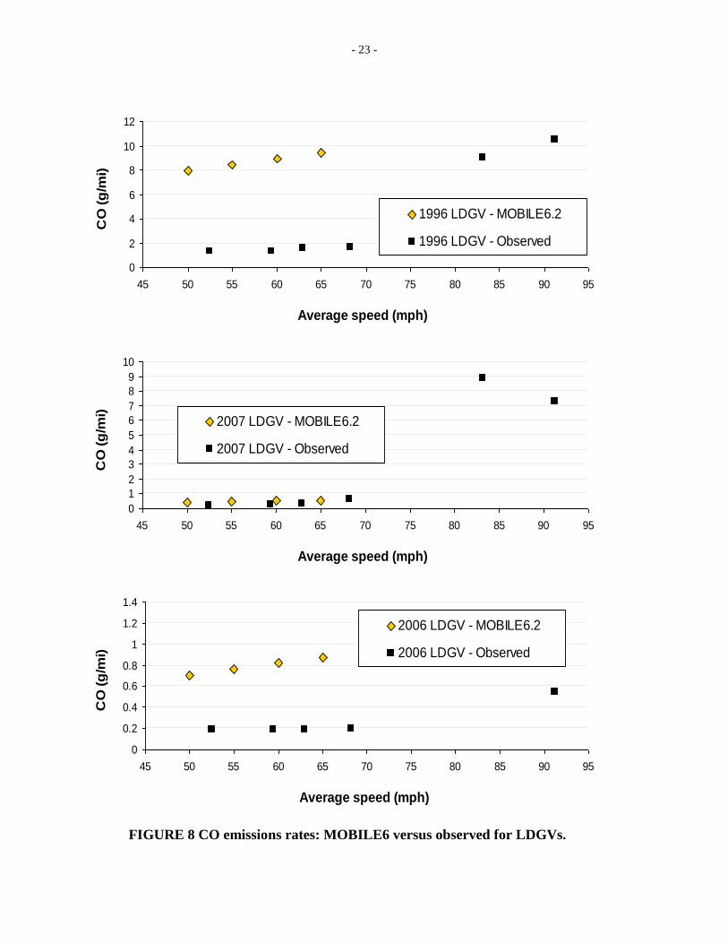
CO Emissions

Figures 8 to 10 show the CO emissions rates for the individual light-duty gasoline vehicles,

medium-duty diesel trucks, and heavy-duty diesel trucks respectively. The figures show the

emissions rates produced by MOBILE6 as well as the observed rates produced using the

regression models.

In Figure 8 the observed and MOBILE6 rates for the 1996 Nisan Altima show the same

general trend up to 65 mph although the observed rates are significantly lower than those

produced by MOBILE6.However, the observed results also show that the CO emissions rate

increases at a faster rate at speeds higher than 65 mph for this car. The results for the 2006 Ford

Mustang show very similar results for observed and MOBILE6 rates up to 65 mph, beyond

which there is a steep increase in the observed emissions rates. For the 2007 Jeep Liberty, the

observed CO emissions rates are much lower than for the MOBILE6 case, while showing the

same general trend.

Figure 9 shows that the observed CO emissions rates are overall higher than the

MOBILE6 emissions rates for all the three medium-duty trucks. The MOBILE-6 emissions for

the 2002 Dodge Ram and the 2006 Ford F-250 are similar, and show an increasing trend. The

observed values for both are flatter than the MOBILE6 rates, with a slightly decreasing trend for

the 2002 vehicle, especially beyond 75 mph, and a slightly increasing trend beyond 75 mph for

the Ford F-250. Finally, the observed rates and the MOBILE6 rates for the 2007 Chevrolet

Silverado are different, with MOBILE6 showing lower rates and a flat trend, compared to higher

rates and a slightly increasing trend in case of the observed values.

Figure 10 shows that the comparison between the MOBILE6 rates and the observed rates

are similar for all three heavy-duty trucks (2001 with a CAT C15 engine, 2002 with a Detroit

engine, and 2006 with a Cummins 870 engine). The observed emissions rates are slightly higher

than the MOBILE6 rates and exhibit a slightly decreasing trend up to 65 mph, beyond which the

values tend to decrease slightly for the 2001 and 2002 model trucks, and increase slightly in the

2006 model.

- 23 -

FIGURE 8 CO emissions rates: MOBILE6 versus observed for LDGVs.

0

2

4

6

8

10

12

45 50 55 60 65 70 75 80 85 90 95

Average speed (mph)

CO

(g

/mi)



0

1

2

3

4

5

6

7

8

9

10

45 50 55 60 65 70 75 80 85 90 95

Average speed (mph)

CO

(g

/mi)



0

0.2

0.4

0.6

0.8

1

1.2

1.4

45 50 55 60 65 70 75 80 85 90 95

Average speed (mph)

CO

(g

/mi)



- 24 -

FIGURE 9 CO emissions rates: MOBILE6 versus observed for HDDV2bs.

0

0.2

0.4

0.6

0.8

1

1.2

45 50 55 60 65 70 75 80 85 90 95

Average speed (mph)

CO

(g

/mi)



0

0.2

0.4

0.6

0.8

1

1.2

1.4

45 50 55 60 65 70 75 80 85 90 95

Average speed (mph)

CO

(g

/mi)



0

0.2

0.4

0.6

0.8

1

1.2

45 50 55 60 65 70 75 80 85 90 95

Average speed (mph)

CO

(g

/mi)



- 25 -

FIGURE 10 CO emissions rates: MOBILE6 versus observed for HDDV8bs.

0

1

2

3

4

45 50 55 60 65 70 75 80 85 90 95

Average speed (mph)

CO

(g

/mi)



0

1

2

3

4

45 50 55 60 65 70 75 80 85 90 95

Average speed (mph)

CO

(g

/mi)



0

1

2

3

4

45 50 55 60 65 70 75 80 85 90 95

Average speed (mph)

CO

(g

/mi)



- 26 -

THC Emissions

Figures 11 to 13 show the total hydrocarbon (THC) emissions rates for the individual light-duty

gasoline vehicles, medium-duty diesel trucks, and heavy-duty diesel trucks respectively. The

figures show the emissions rates produced by MOBILE6 as well as the observed rates produced

using the regression models.

Figure 11 shows that as for other pollutants, the observed and MOBILE6 rates for the

1996 Nisan Altima show the same general trend up to 65 mph although the observed rates are

lower than those produced by MOBILE6. The observed results also show that the THC

emissions rate increases at speeds higher than 65 mph for all three vehicles. The results for the

2006 Ford Mustang show the observed rates to be much lower than the MOBILE6 emissions

rates. However, the observed emissions rates for the Ford Mustang are considerably lower than

that produced by MOBILE6. The THC emissions rates for the 2007 Jeep Liberty are

approximately the same for the observed and MOBILE6 cases.

Figure 12 shows that the observed emissions rates are very similar to the MOBILE6 rates

for the 2002 Dodge Ram, and exhibit a slightly decreasing trend, even beyond 65 mph. The

results for the 2006 Ford F-250 and the 2007 Chevrolet Silverado, however, show higher

observed rates than MOBILE6 rates, and exhibit a slightly increasing trend compared to the

MOBILE6 values that remain fairly flat.

Figure 13 shows for the 2001 and 2002 model trucks, the MOBILE6 emissions rates are

higher than the observed rates, while for the 2006 model, the observed rates are higher.

However, the same general trends are observed for all the three engines – the MOBILE rates

remain flat, while the observed rates are flat up to around 70 mph, beyond which there is a

tendency for the rate to increase.

- 27 -

FIGURE 11 THC emissions rates: MOBILE6 versus observed for LDGVs.

0

0.05

0.1

0.15

0.2

0.25

0.3

45 50 55 60 65 70 75 80 85 90 95

Average speed (mph)

TH

C (

g/m

i)



0

0.05

0.1

0.15

0.2

45 50 55 60 65 70 75 80 85 90 95

Average speed (mph)

TH

C (

g/m

i)



0

0.005

0.01

0.015

0.02

0.025

0.03

0.035

45 50 55 60 65 70 75 80 85 90 95

Average speed (mph)

TH

C (

g/m

i)



- 28 -

FIGURE 12 THC emissions rates: MOBILE6 versus observed for HDDV2bs.

0

0.05

0.1

0.15

0.2

0.25

0.3

45 50 55 60 65 70 75 80 85 90 95

Average speed (mph)

TH

C (

g/m

i)



0

0.05

0.1

0.15

0.2

0.25

0.3

45 50 55 60 65 70 75 80 85 90 95

Average speed (mph)

TH

C (

g/m

i)



0

0.02

0.04

0.06

0.08

0.1

0.12

0.14

0.16

45 50 55 60 65 70 75 80 85 90 95

Average speed (mph)

TH

C (

g/m

i)



- 29 -

FIGURE 13 THC emissions rates: MOBILE6 versus observed for HDDV8bs.

0

0.1

0.2

0.3

0.4

0.5

0.6

45 50 55 60 65 70 75 80 85 90 95

Average speed (mph)

TH

C (

g/m

i)



0

0.1

0.2

0.3

0.4

0.5

45 50 55 60 65 70 75 80 85 90 95

Average speed (mph)

TH

C (

g/m

i)



0

0.1

0.2

0.3

0.4

0.5

45 50 55 60 65 70 75 80 85 90 95

Average speed (mph)

TH

C (

g/m

i)



- 30 -

Expansion of MOBILE6 Rates

The main goal of this project was to develop emissions rates for speeds of 65 mph and higher so

that MOBILE6 rates can be expanded for higher speeds. Figures 5 through 13 show the results

for the individual vehicles for both MOBILE6 and those developed from the observations. In

expanding the MOBILE6 curve, it was decided to focus only on the observed rates for speeds of

65 mph and higher. Furthermore, it was decided to develop weighted averages for the observed

emissions rates of these higher speeds. The weighted averages were based on vehicle registration

data for Texas (13). For example, in the case of LDGVs, the relative composition (fractions) of

1996, 2006, and 2007 vehicles were considered. Table 6 shows the percentage registered

vehicles in each of the categories used in this study. Based on the vehicle registration data the

relative proportions of the different model year could be determined. These proportions were

then used to weigh the observed data points for the three vehicles to develop weighted average

rates for speeds of 65 mph and higher for each of the three vehicle classes.

TABLE 6 Percentage Registered Vehicles per Category

Category Fuel type Year Percentage registered

LDGV Gasoline 1996 5%



HDDV2b Diesel 2002 8%






Regression equations were developed with the weighted average rates to represent the

expansion of the emissions rates above 65 mph for each of the classes. Equations 2 through 4

show the formulation of these equations for LDGV, HDDV2b, and HDDV8b, respectively.

0.0144( 65)y x (r2 = 0.981) (2)

0.0121( 65)y x (r2 = 0.632) (3)

0.1459( 65)y x (r2 = 0.966) (4)

Where:

x = speed in mph: and

y = NOx emissions rate in g/mile.

The above process was illustrated by expanding MOBILE6 rates above 65 mph for the

three vehicle classes. For demonstration purposes, MOBILE6 rates for the San Antonio, Texas

area were used. These rates were developed as part of emissions inventory determination using

the fleet mix for the San Antonio area (14).The expansion slopes of Equations 2 through 4 were

then used to expand these composite MOBILE6 rates.

- 31 -

Figures 14,15 and 16 shows the MOBILE6 rates for the three vehicle classes as well as

the expansions to higher speeds for NOx, CO, and THC respectively. The figures show that the

observed emissions rate for LDGVs at speeds above 65 mph increase at a higher rate than the

trend produced by MOBILE6. In the case of HDDV2bs, MOBILE6 shows a strong increasing

trend and the observed rates for higher speeds show a slight decreasing trend. This result is

somewhat surprising considering the increasing trend of MOBILE6 results. For HDDV8bs the

observed rates increase at a lower rate than MOBILE6 for higher speeds.

Figure 8 shows that the expansion slopes can easily be applied to any set of MOBILE6

rates regardless of area. The same process described in this report can be used to develop

expansion slopes or curves for the other vehicle classifications.

- 32 -

FIGURE 14 Expansion of MOBILE6 Emissions Rates: NOx.

0

5

10

15

20

25

30

35

0 10 20 30 40 50 60 70 80 90 100

Average speed (mph)

NO

x (

g/m

i)

HDDV8b - MOBILE6.2

Suggested Trend

0

0.2

0.4

0.6

0.8

1

1.2

1.4

1.6

1.8

0 10 20 30 40 50 60 70 80 90 100

Average speed (mph)

NO

x (

g/m

i)

LDGV - MOBILE6.2

Suggested Trend

0

1

2

3

4

5

6

0 10 20 30 40 50 60 70 80 90 100

Average speed (mph)

NO

x (

g/m

i)

HDDV2b - MOBILE6.2

Suggested Trend

- 33 -

FIGURE 15 Expansion of MOBILE6 Emissions Rates:CO.

0

2

4

6

8

10

12

14

16

18

0 10 20 30 40 50 60 70 80 90 100

Average speed (mph)

CO

(g

/mi)

HDDV8b - MOBILE6.2

Suggested Trend

0

5

10

15

20

25

30

35

0 10 20 30 40 50 60 70 80 90 100

Average speed (mph)

CO

(g

/mi)

LDGV - MOBILE6.2

Suggested Trend

0

0.5

1

1.5

2

2.5

3

3.5

4

4.5

5

0 10 20 30 40 50 60 70 80 90 100

Average speed (mph)

CO

(g

/mi)

HDDV2b - MOBILE6.2

Suggested Trend

- 34 -

FIGURE 16 Expansion of MOBILE6 Emissions Rates: THC.

0

0.2

0.4

0.6

0.8

1

1.2

1.4

1.6

1.8

2

0 10 20 30 40 50 60 70 80 90 100

Average speed (mph)

TH

C (

g/m

i)

HDDV8b - MOBILE6.2

Suggested Trend

0

1

2

3

4

5

6

7

8

9

0 10 20 30 40 50 60 70 80 90 100

Average speed (mph)

TH

C (

g/m

i)

LDGV - MOBILE6.2

Suggested Trend

0

0.1

0.2

0.3

0.4

0.5

0.6

0 10 20 30 40 50 60 70 80 90 100

Average speed (mph)

TH

C (

g/m

i)

HDDV2b - MOBILE6.2

Suggested Trend

- 35 -

CONCLUSIONS

The goal of this project was to develop emissions rates for three classes of vehicles (light-duty

gasoline vehicles, medium-duty trucks, and heavy-duty trucks) for speeds above 65 mph to

enable the expansion of MOBILE6 rates to higher speeds. The study generated actual emissions

data obtained through PEMS equipment mounted on vehicles driven through pre-determined

drive cycles on a test track.

The study produced the following results:

A compilation of MOBILE6 drive cycles for speeds from 40 mph to 65 mph and newly

developed cycles for speeds from 65 mph to 90 mph;

Drive cycles for vehicles to be driven on the test track so emissions could be measured for

all the required speed, acceleration, deceleration, and idling events;

Emissions rates for all the test vehicles while driving the pre-determined cycles;

MOBILE6 rates for each of the test vehicles used in the study;

Regression models for estimating emissions of the different vehicles and vehicle classes

for the various speed, acceleration, deceleration, and idling events;

Estimation of emissions for speeds from 40 to 65 mph based on MOBILE6 cycles and for

65 mph to 85 mph based on the newly developed cycles;

Comparison of observed rates with MOBILE6 rates; and

Expansion curves to extend MOBILE6 emissions rates to speeds above 65 mph.

It was found that for speeds from 40 mph to 65 mph the observed rates for light-duty

gasoline vehicles follow the same trend as MOBILE6 whereas those of medium- and heavy-duty

trucks show a flat trend as opposed to MOBILE6’s increasing trend. For speeds above 65 mph

the rate of increase for light-duty vehicles is higher than the trend in MOBILE6 whereas the rate

for medium-duty trucks is considerably less and the rate of increase for heavy-duty trucks is

slightly less than that of MOBILE6.

Expansion curves were developed for speeds above 65 mph for each of the three vehicle

classes. These curves can be applied to any set of MOBILE6 rates regardless of area. For

illustration purposes, it was shown how the emissions rates for the San Antonio area can be

expanded using the expansion curves.

The findings from the study will enable transportation and air quality planners to more

reliably assess impacts associated with high speed operation already existing on freeways and

tollways as well as future facilities that will begin to appear in MTPs in the near future.

ACKNOWLEDGEMENTS

This research effort was funded by the Houston Advanced Research Center (HARC) with

funding from the EPA, Texas State Legislature Earmark Funding, and the Mid-Atlantic

University Transportation Center (MAUTC). In particular the authors would like to thank David

Hitchcock of HARC for his oversight and support. The authors would also like to thank the

following TTI researchers for their contributions without which this study would not have been

possible – Edward Brackin, Marty Boardman, Dennis Perkinson, L.D. White, Rafael Aldrete,

Rajat Rajbhandari, Jeffrey Shelton, and Arturo Bujanda.

REFERENCES

- 36 -

1. Keep Texas Moving. http://www.keeptexasmoving.com/, accessed July 2007.

2. Pecos Economic Development Corporation. http://www.pecos.net/news/pedc/whoweare.htm,

accessed July 2007.

3. Sensors' Emissions Measurement Technology. http://www.sensors-inc.com/semtech.htm,

accessed July 2007.

4. The Montana System. http://www.cleanairt.com/content.aspx?iid=179, accessed July 2007.

5. Environmental Protection Agency. Technical Guidance on the Use of MOBILE6 for Emission

Inventory Preparation. U. S. Environmental Protection Agency, Office of Air and Radiation,

Washington, D.C., January 2002.

6. Environmental Protection Agency. Draft Design and Implementation Plan for EPA’s Multi-

Scale Motor Vehicle and Equipment Emission System (MOVES). EPA 420-P-02-006. U. S.

Environmental Protection Agency, Office of Air and Radiation, Washington, D.C., October

2002.

7. Carlson, T.R., and T.C. Austin. Development of Speed Correction Cycles. SR97-04-01. U.S.

Environmental Protection Agency. 1997.

8 Ahn, K., H. Rakha, A. Trani, and M. Van Aerde, Estimating vehicle fuel consumption and

emissions based on instantaneous speed and acceleration levels. Journal of

Transportation Engineering, 2002. 128(2): p. 182-190.

9 Ahn, K., H. Rakha, A. Trani, and M. Van Aerde, Estimating vehicle fuel consumption and

emissions based on instantaneous speed and acceleration levels. Journal of

Transportation Engineering, 2002. 128(2): p. 182-190.

10

Rakha, H. and K. Ahn, Integration modeling framework for estimating mobile source

emissions. Journal of transportation engineering, 2004. 130(2): p. 183-193.

11

Jimenez, J.L., Understanding and Quantifying Motor Vehicle Emissions with Vehicle Specific

Power and TILDAS Remote Sensing, in The Department of Mechanical Engineering.

1999, The Massachusetts Institute of Technology.

12

Simonoff, J.S., Smoothing Methods in Statistics. 1996: Springer.

13. Development and Production of Virtual Link, On-Road Mobile Source, Episode Specific

Emissions Inventories for All 254 Texas Counties for Analysis Years 2005 and 2006. Prepared

for the Texas Commission on Environmental Quality, Study No. 402231-08. Texas

Transportation Institute, The Texas A&M University System, College Station, Texas, June 2007.

http://www.keeptexasmoving.com/

http://www.pecos.net/news/pedc/whoweare.htm,%20accessed%20July%202007

http://www.pecos.net/news/pedc/whoweare.htm,%20accessed%20July%202007

http://www.sensors-inc.com/semtech.htm,%20accessed%20July%202007

http://www.sensors-inc.com/semtech.htm,%20accessed%20July%202007

http://www.cleanairt.com/content.aspx?iid=179

- 37 -

14. Development of 2005 Three-Year Cycle, On-Road Mobile Source Actual Annual, and

Summer Season Weekday Emission Inventories for the San Antonio Early Action Compact Area

Counties. Prepared for the Texas Commission on Environmental Quality, Study No. 402231-02.

Texas Transportation Institute, The Texas A&M University System, College Station, Texas,

August 2006.

in s titu te tr a n s p o rt a tio n te x a s · the goal of this project was to develop emissions...

Documents