Integrated Lot-sizing and Scheduling for Just-In-Time Production

of Complex Assemblies with Finite Set-ups

Muhammad F. Anwar, Rakesh Nagi�

Department of Industrial Engineering, 342 Bell Hall

State University of New York at Bu�alo, Bu�alo, NY 14260

Abstract

This paper addresses the integrated scheduling and lot-sizing problem in a manufacturing

environment which produces complex assemblies. Given the due-dates of the end items, the

objective is to minimize the cumulative lead time of the production schedule (total makespan)

and reduce set-up and inventory holding costs. A JIT production strategy is adopted in which

production is scheduled as late as possible (to minimize WIP costs), but without backlogging

end items. The integrated scheduling and lot-sizing problem within such an environment has

been formulated and is NP hard. An e�cient heuristic is developed that schedules operations

by exploiting the critical path of a network and iteratively groups orders to determine lot-

sizes that minimize the makespan as well as set-up and holding costs. The performance of

the proposed heuristic is evaluated and numerical results are presented comparing the savings

achieved in makespan and cost over a lot-for-lot production strategy, and scheduling using an

existing heuristic. More generally, this study demonstrates that lot-for-lot production in small

batches may not be the best JIT strategy in an assembly environment with �nite set-ups.

Keywords: Complex Assemblies, Just-in-time (JIT), Makespan, Lot-sizing, Scheduling.

�To whom correspondence should be addressed. Tel: 1-(716)-645-2357 x 2103, Fax: 1-(716)-645-3302, Email:nagi@eng.bu�alo.edu

1 Introduction

In today's highly competitive environment, manufacturing strategy is changing from mass to small

batch production in order to incorporate rapid changes in customers preferences and demand. Due

to the continual pressure imposed by the competitive market, customers do not wish to receive

products in a large quantity at the same time. They would like to spread their demand over a

period of time in order to minimize their tied up capital in equipment or inventories. On the other

hand, producers also want to minimize their inventories, including Work-In-Process (WIP), as well

as total production costs. When manufacturing small batches of similar or customized complex

assemblies, if set-up costs and times are not negligible, then multiple replications of the set-ups over

the planning horizon would result in signi�cant expenses. Therefore, in this environment, Just-In-

Time (JIT) production of products and their sub-assemblies cannot be performed in a lot-for-lot

manner. For a manufacturing �rm to be competitive, the required quantity of the products needs

to be delivered on time and at minimal cost. The major components of the production cost which

do not add value to the product, and should be reduced, are set-up cost, inventory holding cost

and work-in-process cost. Due to the diversity of products and staggered demand, the production

planning and scheduling problems in small batch manufacturing become very complex. More

speci�cally, in a manufacturing environment which produces small batches of complex assemblies,

it becomes very di�cult to control costs and meet due dates.

The production environment addressed in this study is a manufacturing facility that manufac-

tures complex assemblies in small batches. Within such an environment, in planning and scheduling,

many decisions have to be made related to lot-sizing, timing, and inventory (Zahorik et al., 1984).

Even in simple, small dimensional problems the number of scheduling alternatives is quite large,

and therefore, good heuristic approaches are highly desirable (Agrawal et al., 1995).

This study focuses on: (i) lot-sizing and order grouping to minimize set-up and inventory

holding costs, and (ii) operation scheduling, for just-in-time production of complex assemblies

under multiple capacity constraints. These are critical issues for large and complex assembly

manufacturing in which �nished product cycle-times range between several months to two years.

The objective is to reduce the cumulative lead time of the production schedule (total makespan)

and minimize set-up and inventory holding costs in order to \deliver these assemblies at the right

time and with the right cost." To achieve these objectives, a JIT production approach is adopted

which delays operations as late as possible, and initially operations are considered using a lot-for-lot

strategy. Then the proposed heuristic is employed for simultaneous lot-sizing and scheduling to

minimize cycle-time as well as set-up and inventory holding costs.

The method proposed in this study is a two-phase heuristic that addresses the case of complex

assembly manufacturing, in which both precedence and capacity constraints are critical. In the

�rst phase, the proposed heuristic schedules operations by exploiting the critical path to minimize

makespan on a lot-for-lot basis. In the second phase, the heuristic iteratively groups orders to

obtain lot-sizes that further reduce the makespan, set-up and holding costs.

1

The paper is organized as follows. In section 2, a literature review is presented. In section 3,

the problem description and the mathematical formulation of the problem are provided. In section

4, the proposed heuristic is presented. In section 5, the results of numerical tests, and the savings

in makespan as well as cost achieved by our proposed heuristic are presented. Finally in section 6,

conclusions of this study are presented.

2 Background

Materials Requirements Planning (MRP) is commonly used in industry to determine production

schedules in a multi-stage manufacturing environment. Production requirements of an end item

are translated into known production (or purchase) quantities and timing of components, based on

bill-of-materials and lead time information (Orlicky, 1975).

MRP ignores detailed shop- oor capacity constraints and usually assumes �xed production lead

time (independent of lot-size and current shop work-load), which is not realistic. The considera-

tion of capacity constraints is important in scheduling problems. Some production planning and

scheduling systems that perform the function of MRP in a capacitated environment have also been

proposed. These systems (Reiter, 1966; Godin and Jones, 1969; Goldratt, 1980) do not perform

satisfactorily in a multi-stage production environment with more than one capacity constraint, with

multiple objectives of reducing cycle time and production costs. The OPT system (Levulis, 1985),

which employs proprietary algorithms, identi�es the bottleneck resources through simulation and

uses heuristic methods to load these resources during periods when they are idle. Comparisons of

these proprietary systems with conventional production scheduling methods are not available.

The following discussion of the literature focuses on: (i) lot-sizing in a multi-level environment,

(ii) job-shop scheduling of multi-level products, and (iii) lead time, work-in-process (WIP) cost and

just-in-time (JIT) production. All these areas are relevant to the problem of producing complex

assemblies with shortest possible makespan and at minimal cost.

2.1 Lot-sizing

Single-item, Multi-level uncapacitated environment: For large and complex product struc-

tures, in a single-item, multi-level environment, the Wagner-Whitin algorithm (1958) which is op-

timal for single-level, and the heuristics Part Period Balancing (DeMatteis, 1968), Silver and Meal

(1973), Least Unit Cost (Love, 1979), all use single level information in order to determine sequen-

tially the lot-scheduling pattern without considering any capacity constraints (Afentakis et al.,

1984). The optimal algorithm developed by Afentakis et al. (1984) solves a medium sized lot-sizing

problem for a single product structure of assembly type in an uncapacitated environment. Some

earlier work was also performed by Zangwill which includes, the single resource network model

(Zangwill, 1968), various dynamic programming formulations to consider the cases of backlogging

(Zangwill, 1969), concave costs (Zangwill, 1968) and multiple products (Zangwill, 1977) in an unca-

2

pacitated environment. The optimal method of Crowston and Wagner (1973) considered the case of

multi-stage assembly systems for multiple predecessors but only a single successor, while Crowston

et al. (1973) considered the same problem with the constraint that lot-sizes remain time invariant

in the above environment. The uncapacitated environment is of limited relevance in real-world

applications.

Single-item, Multi-level capacitated environment: Chung et al. (1994) combined dynamic

programming with a branch-and-bound procedure to solve the single-item capacitated lot-sizing

problem in a multi-level environment. Kirca (1990) developed a dynamic programming-based al-

gorithm to solve the lot-sizing problem in the above environment. He suggested that an e�cient

algorithm in such an environment could be an important part of a multi-product scheduling al-

gorithm. Again, the above environment is not relevant to complex assembly manufacture which

require production and lot-sizing of multiple end items with possibly shared components.

Multi-item, Multi-level uncapacitated environment: Blackburn and Millen (1982) pro-

posed a heuristic to address the problem of lot-sizing in a multi-item, multi-level, uncapacitated

environment. The TOPS algorithm (Coleman and McKnew, 1990) and the STIL algorithm (Cole-

man and McKnew, 1991) give better results than Wagner-Whitin (1958) for the sequential applica-

tion in multi-item, multi-level uncapacitated problems, but they do not guarantee optimal solutions

for individual items. Although, the lot-sizing problem in multi-item, multi-level environment is very

relevant to complex assembly manufacture, the lot-sizes obtained under the assumption of in�nite

capacity are seldom feasible in a capacitated production environment.

Multi-item, Multi-level capacitated environment: Steinberg and Napier (1980) modeled

the multi-item, multi-level capacitated lot-sizing problem as a generalized network problem and

relaxed the single successor restriction. They presented the optimal Integer Programming solution

to lot-sizing but only for three products and four-levels. To solve larger problems, they have

to relax capacity constraints. The heuristic developed by Tempelmeier and Helber (1994) uses

sequential application of Dixon-Silver lot-sizing algorithm (1981) to solve the multi-item, multi-

level capacitated lot-sizing problem. The e�ect of multi-level interactions is not considered in this

study, therefore, the lot-sizes obtained at one level may not be optimal at other levels. Due to

complex combinatorial structure, computationally lot-sizing problems in multi-stage systems are

extremely di�cult (Afentakis et al., 1984).

In the multi-level environment, when the lot-sizes are computed at each level using single-level

lot-sizing methods without considering the e�ect of multi-level interactions, the lot-sizes which are

optimal at one level may not be optimal at other levels. Also, the lot-sizes that are determined under

the assumptions of in�nite capacity, are often infeasible with respect to the available production

capacity. Further, in the multi-item, multi-level capacitated environment, at times detailed capacity

is considered only at one level which is usually the end item level. Even the lot-sizing techniques

3

which consider capacity at all levels, do so in a production planning sense which does not guarantee

a realizable schedule. Finally, the problem of minimization of makespan is not addressed which is a

critical issue in the manufacture of large and complex assemblies. Therefore, the lot-sizing problem

in multi-item, multi-level environment under multiple capacity constraints, needs to be addressed

not only at the planning level, but also at the scheduling level.

2.2 Job-shop Scheduling of Multi-level Products

In the �eld of scheduling, the literature is vast, and it has been reviewed and classi�ed by many au-

thors. Panwalker and Iskander (1977) analyzed and summarized di�erent priority rules presented in

the literature. Rodammer and White (1988) surveyed di�erent methods used in production schedul-

ing. Blazewicz et al. (1991) have compiled a number of mathematical programming formulations

for scheduling. McCarthy and Liu (1993) have listed the various types of scheduling problems and

also the well known solution methods proposed in the literature. For the n-job, m-machine job-

shop problem, various approaches have been proposed for the minimization of makespan, including

heuristic methods (Ashour, 1967; Adams et al., 1988), and those based on mixed integer linear

program (MILP) (Greenberg, 1968), and branch and bound (Ashour and Hiremath, 1973; Lageweg

et al., 1977; Baker and McMohan, 1985; Carlier and Pinson, 1989).

The scheduling problem and its complexity in single-stage, multi-item capacitated production

environment is considered by many authors (Elmaghraby, 1978; Delporate and Thomas, 1977; Lam-

brecht and Vanderveken, 1979; Dixon and Silver, 1981; Baker et al., 1978; Kirca and Kokten, 1994).

The single stage problem has been shown to be computationally very complex and the problem

is accepted to be NP-hard (Lenstra and Rinnooy Kan, 1979). The \Shifting Bottleneck" method

of Adams et al. (1988) has shown superior performance for realistic sized problems by schedul-

ing a given set of operations on their respective work centers. While this method is applicable to

single-level product structures, it cannot be easily extended to multi-level products such as complex

assemblies because it does not allow for precedence relationships between routings. Dauzere-Peres

and Lasserre (1994) addressed the integrated lot-sizing and scheduling problem, and proposed a

two-level iterative procedure to compute the best possible (feasible) schedule in a job-shop environ-

ment. This is accomplished by alternatively solving a lot-sizing problem for a given sequence of jobs

that share a common resource, and a scheduling problem for a �xed lot-size. Again, this method

cannot be extended easily to multi-level environment for the same reasons described earlier. In sum-

mary, the integrated lot-sizing and scheduling problem in a multi-level, multi-product environment

under multiple capacity constraints has not been addressed adequately in the literature.

2.3 Lead Time, WIP Cost and JIT Production

Lead time determination is related to capacity planning and its consideration is very important

in scheduling problems. Karmarkar (1989) noted that WIP and lead time related costs are signif-

icant parts of total manufacturing costs even when capacity utilization is less than 100 percent.

4

He suggested that lot-sizes are associated with lead times and are quite di�erent from those of

conventional EOQ models (Karmarkar, 1987).

By reducing lot-sizes, the lead time can be reduced resulting in lower WIP costs, and this is

the movement towards JIT production strategy (Schniederjans, 1993). Scheduling in small lot-sizes

would enable a producer to respond more quickly to customers' demand for a variety of products

without holding large inventories. However, in doing so, total set-up costs might increase which is

also undesirable.

Billington et al. (1983) focused on determining required lead times for only the constrained

resources. They classi�ed multi-level product structures into four types, and proposed a two stage

approach for the multi-level job-shop scheduling problem. In the �rst stage the product structure

is compressed using a heuristic based on bottleneck resource identi�cation and lot-sizing. In the

second stage an MILP method is employed to �nd the optimal makespan for the reduced prob-

lem. They also suggested that the key to e�cient production scheduling is simultaneous lead time

determination and capacity planning. However, no comparison is available between the makespan

obtained by the compressed product structure and the minimum makespan of the complete product

structure.

The work of Miltenburg and Sinnamon (1992, 1989) considered mixed model scheduling for

assembly lines in JIT production systems. WIP costs were controlled by determining constant

usage rates of items at each level of production. To minimize variation in usage rate, products were

sequenced in very small lots. However, this method could be cost e�ective only when set-up costs

are negligibly small.

Agrawal et al. (1995) addressed the problem of scheduling operations in a manufacturing

facility which produces large assemblies. They assumed known lot-sizes of end items and JIT

production, and developed an algorithm to minimize the lead time and WIP costs by considering

both precedence and capacity constraints as critical. The e�ect of lot-sizing or order grouping is

not taken into account in this study.

Since di�erent lot-sizes result in di�erent lead times, WIP costs, set-up costs and holding costs,

the optimal lot-size has to be determined to reduce set-up and holding costs while minimizing the

production lead time at the same time. The suggested topic is to study the three way interaction

of lead time, lot-sizing, and actual capacity constraints, in a manufacturing environment which

produces complex assemblies, to optimize the scheduling process.

3 Problem Formulation

A manufacturing facility that produces complex assemblies is considered which consists of w work-

centers fW1;W2; :::Wwg. Each work-center WY may consists of fY functionally identical machines.

In the production environment raw materials undergo a series of di�erent operations where value

is added at each step, and remain in a semi-�nished (intermediate) state until they are �nally

transformed into �nished products. We consider a set of �nal assemblies, Pf = fp1; p2; :::; pnfg,

5

a set of semi-�nished parts, Ps, and a set of purchased parts (raw material), Pr. Semi-�nished

parts are considered as inventory items. The set of manufactured (or make) parts includes all

the �nal assemblies and the semi-�nished parts, and is represented by Pm = Pf [ Ps. Each make

part pi 2 Pm, is processed through a unique sequence of operations (or routing) < Ojl >sjl=1,

and each �nished product pi has a unique Bill-of-Material (BOM) which represents its assembly

structure. The sample BOMs of two �nished products, A and B are shown in Fig. 1 (set-up times

are exaggerated a little bit in order to later show the e�ect of multiple set-ups on the makespan).

Further, a delivery schedule consists of a list of �nished products, their associated quantities

and due-dates. Let Di and di represent the due-date and order quantity respectively, of product pi

(pi 2 Pf ). Furthermore, a back-to-back production strategy is adopted in which an entire batch of

an item is processed by a certain machine before the next operation can start. Finally, to formulate

the problem, the following assumptions are made:

� Machines are assumed to be reliable.

� A machine can perform at most one operation at a time.

� An operation can be performed on at most one machine at a given time.

� Preemption of operations is not permitted.

� Processing times of all operations and due-dates of all �nal products are deterministic and

known.

� Backlogging is not permitted.

3.1 Network Representation of Precedence Relationships

The precedence relationship among operations of each end item may be obtained from its BOM

and make part routings, and can be represented by a precedence network. The network may also

incorporate component lead time o�sets, which are possible due to the fact that production of

a component pk of part pi can be completed (after the production of pi has begun) until pk is

actually needed in a certain operation of the routing of pi. For the calculation of lead time o�sets

see Agrawal et al. (1995).

Figure 2 represents the precedence network of operations corresponding to products A and B,

which is obtained from BOM and routing information of Fig. 1. The network shows that operation

B.20 can start only after operations B.10 and C.10 are �nished. Similarly, operation C.10 can start

only after operations D.10 and F.20 are completed. If the lead time o�sets were not used, the

network would change.

A dummy sequence of operation may be used to combine and represent the network of multiple

products as a single network. This is in order to employ the operation network formulation in a

practical case where more than one �nal assemblies are manufactured in the system on a scheduling

horizon. Equivalently, a single multi-level product structure can be generated to combine the

multiple BOMs (see Agrawal et al., 1995).

6

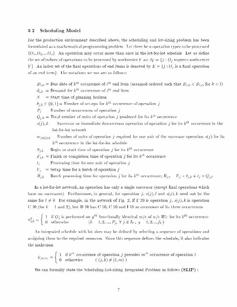
3.2 Scheduling Model

For the production environment described above, the scheduling and lot-sizing problem has been

formulated as a mathematical programming problem. Let there be n operation types to be processed

fO1; O2; :::Ong. An operation may occur more than once in the lot-for-lot schedule. Let us de�ne

the set of indices of operations to be processed by workcenter Y as: IY = fj : Oj requires workcenter

Y g. An index set of the �nal operations of end items is denoted by E = fj : Oj is a �nal operation

of an end itemg. The notations we use are as follows:

Di;k = Due date of kth occurrence of ith end item (assumed ordered such that Di;k < Di;l, for k < l).

di;k = Demand for kth occurrence of ith end item.

S = Start time of planning horizon.

�j;k 2 f0; 1g= Number of set-ups for kth occurrence of operation j.

Pj = Number of occurrences of operation j.

Qj;k = Total number of units of operation j produced for its kth occurrence.

s(j); k = Successor or immediate downstream operation of operation j for its kth occurrence in the

lot-for-lot network.

mjs(j);k = Number of units of operation j required for one unit of the successor operation s(j) for its

kth occurrence in the lot-for-lot schedule.

Sj;k = Begin or start time of operation j for its kth occurrence.

Fj;k = Finish or completion time of operation j for its kth occurrence.

tj = Processing time for one unit of operation j.

Uj = Setup time for a batch of operation j.

Bj;k = Batch processing time for operation j for its kth occurrence; Bj;k = Uj � �j;k + tj �Qj;k .

In a lot-for-lot network, an operation has only a single successor (except �nal operations which

have no successors). Furthermore, in general, for operation j, s(j); l and s(j); k need not be the

same for l 6= k. For example, in the network of Fig. 2, if F.20 is operation j, s(j); k is operation

C.10 (for k = 1 and 2), but D.10 has C.10, C.10 and I.10 as successors of its three occurrences.

�yj;k =

(1 if Oj is performed on yth functionally identical m/c of w/c WY for its kth occurrence0 otherwise (k = 1; 2; :::; Pj; 8 j 2 IY ; y = 1; 2; :::fY )

An integrated schedule with lot-sizes may be de�ned by selecting a sequence of operations and

assigning them to the required resources. Since this sequence de�nes the schedule, it also indicates

the makespan.

jk;lm =

(1 if kth occurrence of operation j precedes mth occurrence of operation l0 otherwise ( (j; k) 6= (l;m) )

We can formally state the Scheduling-Lot-sizing Integrated Problem as follows (SLIP) :

7

Minimize : Max

i; k

fDi;kg � S

Subject to:

Ss(j);k � Fj;k for k = 1; 2; :::; Pj; j = 1; 2; :::; n (1)

Fj;k = Sj;k + (Uj � �j;k + tj �Qj;k) for k = 1; 2; :::; Pj; j = 1; 2; :::; n (2)

jk;lm + lm;jk = 1 for k = 1; 2; :::; Pj; m = 1; 2; :::; Pl; j; l = 1; 2; :::; n; (j; k) 6= (l;m) (3)

Sl;m � Fj;k � ( jk;lm + �yj;k

+ �yl;m

� 3)M for k = 1; :::; Pj; m = 1; :::; Pl;

j; l 2 IY ; y = 1; :::; fY ; Y = 1; :::w; (j; k) 6= (l;m) (4)

Fl;m�Fj;k � ( jk;lm�1)M for k = 1; 2; :::; Pj; m = 1; 2; :::; Pl; j; l = 1; 2; :::; n; (j; k) 6= (l;m) (5)

Fi;k � Di;k for k = 1; :::; Pi; i 2 E (6)

S � Sj;k for k = 1; 2; :::; Pj; j = 1; 2; :::; n (7)

fYXy=1

�yj;k = 1 for k = 1; 2; :::; Pj; j 2 IY ; y = 1; :::; fY ; Y = 1; 2; :::; w (8)

Qj;k � �j;kM for k = 1; 2; :::; Pj; j = 1; 2; :::; n (9)

�j;1 = 1 for j : Pj = 1 (10)

PjXl=1

Qj;l jl;s(j)k �

PjXl=1; l6=k

(mjs(j);lQs(j);l s(j)l;s(j)k)+(mjs(j);k)Qs(j);k for k = 1; 2; :::; Pj; j : s(j) =2 E

(11)

PjXl=1; l6=k

Qi;l il;ik +Qi;k �kXl=1

di;l for k = 1; 2; :::; Pi; i 2 E (12)

8

�j;k 2 f0; 1g for k = 1; 2; :::; Pj; j = 1; 2; :::; n (13)

jk;lm 2 f0; 1g for k = 1; 2; :::; Pj; m = 1; 2; :::; Pl; j; l = 1; 2; :::; n; (j; k) 6= (l;m) (14)

�yj;k 2 f0; 1g for k = 1; 2; :::; Pj; j 2 IY ; y = 1; 2; :::; fY ; Y = 1; 2; :::; w (15)

Qj;k; Sj;k; Fj;k � 0 for k = 1; 2; :::; Pj; j = 1; 2; :::; n (16)

The objective function minimizes the production makespan. Constraint (1) ensures that the

starting time of the kth successor operation cannot be earlier than the �nish time of its immediate

predecessor operation j. Constraint (2) provides the relationship between starting and completion

time for the batch of operation j when it is produced for its kth occurrence. Constraint (3) speci-

�es the unidirectional nature of precedence relationship between two operations in the scheduling

sequence. Constraint (4) is the capacity constraint and provides the relationship between the start-

ing and completion times of any two operations on the same functionally identical machine of a

workcenter WY , the constant M is a very large number. Constraint (5) provides the relationship

between �nish times of two operations that have been speci�ed a precedence from constraint (3).

Constraint (6) indicates that the last operation of the ith end product needs to be completed before

the due date of ith end product for its kth occurrence. Constraint (7) indicates that the start time

of kth occurrence of operation j is greater than the start time of the planning horizon.

Constraint (8) indicates that if an operation Oj is performed on workcenter WY in its kth

occurrence, then it must be performed on only one of its fY functionally identical machines. The

set of constraints (9) ensure that the units can be produced only if a set-up is performed for its kth

occurrence. If Qj;k > 0, then this constraint forces the value of �j;k to be 1, as �j;k is a 0-1 variable.

If Qj;k = 0, the minimization will automatically seek out �j;k = 0. Constraint (10) ensures that a

set-up is always performed if the operation j occurs only once in the lot-for-lot schedule.

Constraint (11) ensures that the production quantity of operation j produced before the start

of its kth successor s(j); k cannot be less than the consumption of j due to its successors scheduled

before and at s(j); k. In a sense, this introduces multiple successor relationships, but results

in a quadratic constraint. Constraint (12) is the no-backlogging constraint and it ensures that

cumulative production quantity of the last operation of the kth occurrence of product i is no less

than its cumulative demand.

Constraints (13), (14) and (15) denote that �j;k ; jk;lm and �yj;k are binary variables. Finally,

constraint (16) indicates that Qj;k, Sj;k and Fj;k are non-negative variables.

Problem (SLIP) is a complex problem, and is assumed without proof to be NP-hard. Therefore,

the existence of a polynomial time algorithm to solve this problem is highly unlikely.

9

4 Scheduling-Lot-sizing Heuristic

Mathematical programming methods, as well as implicit enumeration methods, such as the branch-

and-bound algorithm, can be applied to solve problem (SLIP), only for small dimensional cases.

To address complex assembly structure problems, an e�ective heuristic has been developed. In the

�rst phase, the proposed heuristic schedules the operations on a lot-for-lot basis using the network's

critical path to minimize the makespan. In the second phase, the heuristic iteratively groups orders

to obtain lot-sizes that further reduce the makespan (as well as possibly holding and set-up costs),

and reschedules the modi�ed network using the similar critical path heuristic of phase I.

4.1 Critical Path Concept

Given the BOM structure of a �nal assembly, a continuous sequence of operations that starts from

the �nal operation of the �nished item and terminates at a purchased item is de�ned as a BOM

path. Among the set of BOM paths, the critical path is de�ned as the one along which the sum of

the processing times of all operations is maximal (Agrawal et al., 1995). The critical path would be

the time needed to produce the �nal product if in�nite capacity were assumed. This is typically the

product lead time considered by MRP. However, due to the capacity constraints, the actual product

cycle time is generally greater than the MRP lead time which is computed from the routings of the

make parts and their lot-sizes.

The in�nite capacity critical path is �xed for a given product structure and determines the lower

bound of the makespan. For example, the critical path of the products of Fig. 1, computed from

the operations network of Fig. 2, consists of operations D.10-I.10-B.10-B.20, and the corresponding

makespan is 48 time units. This, however, is the lower bound of the makespan. For a system that

includes only one machine per workcenter, the optimal makespan for the example of Fig. 1 is 111

time units, and the optimal schedule is given in Fig. 3.

A network of operations, similar to that presented in Fig. 2, is used to prioritize operations

and generate a production schedule in the �rst phase of the proposed heuristic, which is similar to

LETSA (Agrawal et al., 1995). The critical path is calculated using a FORWARD pass (or a push

schedule assuming in�nite capacity), and early-start and early-�nish times are recorded for each

operation. Initially, the �rst (dummy operation) and second operations on the in�nite capacity

critical path are scheduled since they also belong to the capacitated critical path. Then considering

precedence relationships, the next operation scheduled is one that has the largest �nish-time, and

the remaining operations are scheduled in the similar manner. In this way the deviation of the

schedule from the lower bound of the makespan is attempted to be minimized.

In the second phase of the heuristic, we determine lot-sizes that are based on \order grouping,"

i.e., some combination of multiple lots of the same part are grouped into aggregated lot(s). This

strategy is adopted for its simplicity, although we recognize that the optimal policy for the problem

SLIP may require lot-splitting. Adopting this, similar parts are merged iteratively. This would

10

change the operations network by combining the same type of operations to a merged operation

and updating its predecessor and successor operations. For example, Fig. 1 shows that both end-

items require part D (which requires one operation D.10) somewhere in their processing sequence.

From Fig. 3 it can be seen that operation D.10 is scheduled three times consecutively, once for

product A and twice for product B. The same is true for operations F.20 and F.10 of part F which

occur once for each product. There are also multiple instances of operation C.10 of part C. After

merging the similar parts their similar operations are combined and their respective predecessor

and successor operations are also added. The changed network is shown in Fig. 4. In the combined

network, the number of successor operations may change from one to more than one depending

upon the merged operations. Accordingly, we modify our previous notation of single successor

s(j); k to a set of successors �(j); k for the kth occurrence of operation j. Further, the number of

occurences Pj of operation j will reduce as its lots are merged. It is noted that this di�ers from

the approaches that consider only the single successor. Again, the critical path is calculated and

scheduling process of phase I is repeated. The resulting schedule is given in Fig. 5, and shows

signi�cant improvement in the makespan from the schedule of Fig. 3. As acknowledged earlier, the

set-up times are exaggerated in this example, hence the signi�cant reduction in makespan.

4.2 Scheduling Lot-sizing Integrated Problem Solving Algorithm (SLIPSA)

The proposed algorithm is a two phase heuristic that addresses the problem (SLIP), and generates

a \good" feasible schedule. It proceeds in a backward scheduling manner similar to MRP, in which

the last operation is scheduled �rst and remaining operations are scheduled backwards in subsequent

steps while respecting all precedence and capacity constraints.

The delivery schedule, product structures and routing data are the inputs to the algorithm,

and are used to construct an integrated operations network. Given this network, a set of feasible

operations is de�ned to include all operations which do not have a successor operation, i:e: F1 =

fOj : �(j); k = ;; j = 1; 2; ::; ng. The �rst phase generates a schedule in four steps: (i) select an

operation from the feasible set F1, (ii) select a speci�c machine from the required workcenter, (iii)

schedule the selected operation, and (iv) update the set of feasible operations.

After scheduling is completed by the �rst phase of the algorithm, the second phase iteratively

groups orders to minimize the makespan (as well as possibly holding and set-up costs). Merging

of two occurrences of similar parts will incur some inventory holding cost. On the other hand,

combining the same type of parts and their respective operations will result savings in set-up time

as well as set-up cost. Therefore, makespan of the schedule after merging a pair of parts is compared

with the previous best schedule; and parts are combined if the schedule results in lower makespan

using the steepest descent or \greedy" approach. Using this approach, all the pairs of similar parts

are merged independently and the makespan of the resulting schedule is calculated and compared

with the previous least makespan schedule. Then the pair which results in the highest saving in

the makespan is selected to be merged. Now this pair is considered as a single part and is deleted

11

from the list of feasible pairs of possible merges, and the network is modi�ed. The list of feasible

pairs is updated and the process is repeated until there is no further improvement in the makespan.

Therefore, by combining the similar parts, as long as it is feasible and results in lower makespan, we

would achieve further reduction in the makespan (and possibly cost) compared to a good lot-for-lot

JIT schedule (see Appendix for cost calculations).

Makespan reduction and lot-grouping is comprised of three steps: (i) identifying the best part

to be merged from the list of feasible, unmerged pair of parts, (ii) merging that pair, and comparing

the makespan of the resulting schedule with previous best schedule, and (iii) accepting the merge

if the new makespan is less than or equal to the makespan of the old schedule. Phase II is repeated

until there is no further reduction in the makespan due to the merging of parts or all the parts have

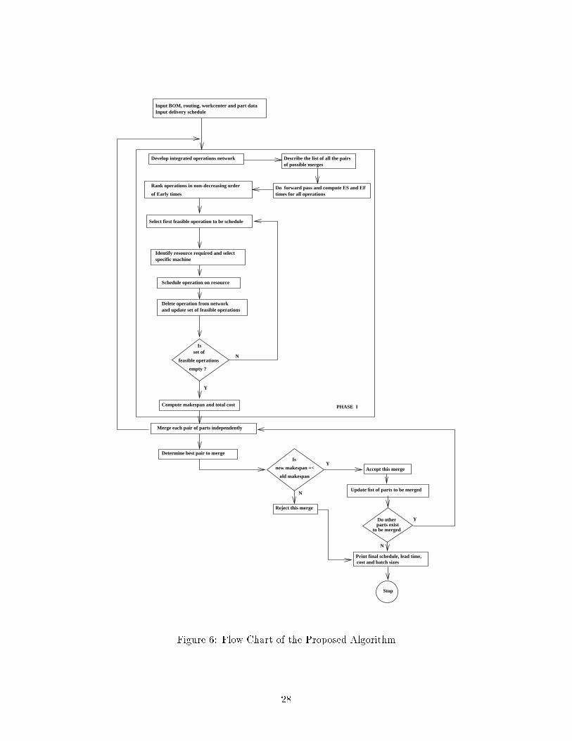
been merged. The step-by-step algorithm is listed below and the ow chart is presented in Fig. 6.

The Algorithm

1. Input manufacturing system data including workcenters, their capacities and number of iden-

tical machines, and product data, i.e. : part master records, BOMs, and the delivery schedule

2. Generate the operation network from the delivery schedule and BOM of end items, and

routing data of their make items

3. De�ne the list of all possible pairs of merges

4. Using forward pass, compute Early Start (ES) and Early Finish (EF) times of all operations

and the critical path

4.1 Rank operations in non-decreasing order of early �nish times

5. De�ne set of feasible operations as F1 = fOj;k : (�(j); k) = ;; j = 1; 2; ::; ng

6. While the feasible list of operations is non-empty, (i.e. F1 6= ;)

6.1 Select the operation that has the largest value of EF time and which also belongs to the

feasible list F1

6.2 Set its �nish time Fj;k equal to: (i) the earliest starting time of operations in �(j); k,

from the partial schedule if �(j); k exists, or (ii) the due date Di;k if operation j is the

last operation of the �nal assembly Pi

6.3 For each identical machine included in the required workcenter

6.3.1 Identify the latest available starting time for the operation Oj;k

6.3.2 If latest available starting time Sj;k = Fj;k �Bj;k , i.e., Sj;k = ideal starting time,

step 6.4

Else select MAX fSj;kg, as the latest available starting time such that the machine

is available during [Sj;k; Sj;k +Bj;k ]

6.3.3 Set Fj;k = Sj;k + Bj;k

6.4 Schedule operation Oj;k at the latest available starting time Sj;k (over multiple machines)

on the corresponding machine

12

6.5 Delete operation Oj;k from the operation network

6.6 Add all operations Ol;m to the feasible list such that �(l); m= ;

7. Compute makespan of the resulting schedule

8. Compute cost of production combining material, labor and work-in-process costs

9. For each pair of duplicate parts that can be merged, do steps 4 through 8

10. Determine the merge that results in the minimal makespan

10.1 If new makespan is � old makespan

10.1.1 Accept this merge

10.1.2 Delete the pair from the list of possible merges and consider this pair of parts as a

single part now

10.1.3 Update the list of possible pairs to be merged; repeat step 9

10.2 Otherwise, reject this merge and stop.

11. Print �nal schedule, lead time, cost and batch-sizes.

5 Results and Discussion

The performance of SLIPSA was evaluated considering a large number of assembly production

examples. Since the problem at hand is NP-hard, optimal results are possible only for small

examples which are of limited interest. For examples of industrial dimension, we have considered

performance over LETSA (Agrawal et al., 1995), which has shown better performance than many

other well-known heuristic methods applied in multi-level assembly scheduling. Another way to

view this performance study is the improvement of phase II over phase I (due to integration of

lot-sizing in scheduling). Three sets of examples were studied. The example sets included large

BOMs corresponding to complex assemblies of three di�erent types. Typical parameters for the

three types of complex assembly BOMs used are presented in Table 1. The last row in this table

indicates the number of pairs of merges due to duplicate parts present in the various cases.

For all the examples, the BOM, part, routing and workcenter structure data were generated

at random from uniform distributions with speci�ed ranges. For each case of the BOM structure

(de�ned in Table 1), the facility consisted three to �ve workcenters, each with one or two identical

machines. The workcenter data included set-up and run costs per unit time (both chosen randomly

between $20/hour and $80/hour). Purchased parts were assigned a cost between $160 and $800.

Routings for manufactured parts were made up of one to four operations, each including set-up

and run times. The run times were chosen randomly between 10 and 30 minutes. For each problem

instance generated, three values of set-up times were chosen by multiplying the run time with a

random multiplier (also called set-up time to run time, or su/ru ratio) from the ranges: 2-3, 20-30,

and 50-60. The following two performance measures were employed:

13

1. Mean percentage improvement in Makespan as compared to LETSA, where

Percentage improvement in makespan = (Makespan)LETSA�(Makespan)SLIPSA(Makespan)LETSA

x 100

2. Mean percentage improvement in Cost as compared to LETSA, where

Percentage improvement in cost = (Cost of Schedule)LETSA�(Cost of Schedule)SLIPSA(Cost of Schedule)LETSA

x 100

We have used two di�erent options for order grouping.

� Best Merge: to group orders iteratively using a steepest descent approach corresponding to

the algorithm outlined in section 4.2.

� All Merge: to group all duplicate orders. It results in signi�cant savings in set-up time and

set-up cost, but may increase WIP and inventory holding costs and also the lead time, due

to extended idle times of parts in the workcenter queues or intermediate storage.

5.1 Makespan comparisons

Three di�erent ratios of set-up time to run-time (su/ru) were used to evaluate the performance of

each model. It is noted that the (su/ru) ratio is also close to the ratio of set-up cost to run cost due

to the labor and machine operating costs per unit time being approximately equal during set-up

and run operations (for these examples). This evaluation test considered: (i) 49 examples of wide

BOMs, (ii) 40 examples of long BOMs, and (iii) 40 examples of large BOMs.

The Mean Percentage improvement in Makespan for each model are presented in Tables 2

through 4. The results indicate that the mean percentage improvement in makespan increases as the

(su/ru) ratio increases for all models. The schedules obtained by SLIPSA resulted in improvement

in makespan over those generated by LETSA for all models in the Best Merge case regardless of the

(su/ru) ratio. In the All Merge case, SLIPSA generally performed better at larger (su/ru) ratios.

However, at smaller (su/ru) ratios the performance of LETSA was better than the All Merge case

of SLIPSA for LARGE and LONG BOMs. This is due to the fact that, for smaller (su/ru) ratios,

the saving in set-up time due to All Merges was not large enough to o�set the increase in the WIP

time due to the advancement and increase in the batch sizes.

It is also noted that in WIDE BOMs, regardless of the (su/ru) ratio, SLIPSA resulted in more

than 10 percent improvement in the makespan in 53 percent of all the examples tested; and at

larger (su/ru) ratios, more than 20 percent improvement in 36 percent of the examples, and more

than 30 percent improvement in the makespan in 22 percent of the examples.

Improvement of more than 10 percent was achieved in 25 (respectively 30) percent of the

examples tested for smaller (su/ru) ratios for LONG (respectively LARGE) BOMs. For larger

(su/ru) ratios, the improvement in makespan was more than 10 percent in 70 (resp. 43) percent

of the examples, more than 20 percent in 30 (resp. 13) percent of the examples, and more than

30 percent in 20 (resp. 7) percent of the examples for LONG (resp. LARGE) BOMs respectively.

This is signi�cant improvement over LETSA.

14

5.2 Cost comparisons

The Mean Percentage savings in Cost for each model are presented in Tables 5 through 7. The

results indicate that for all models, the mean percentage saving in cost generally increases with an

increase in the (su/ru) ratio.

SLIPSA resulted in savings in cost for all models in the Best Merge case, regardless of the

(su/ru) ratio. In the All Merge case, savings in cost were obtained in all models for large (su/ru)

ratios. It is also noted that for smaller (su/ru) ratios, particularly for the All Merge case, savings

in the cost resulted from SLIPSA were less than 10 percent and some times even negative. This

could be the result of signi�cant increase in the WIP cost due to the advancement of a batch to its

merged location, as compared to the savings achieved in cost by reducing multiple set-ups.

For larger (su/ru) ratios, 42 percent of all the examples tested for all the models yielded savings

of more than 10 percent in the cost, 25 percent of all the examples resulted in more than 20 percent

savings, and 13 percent of the examples gave more than 30 percent savings in the cost.

In summary, for the Best Merge option of SLIPSA, 87 percent of the examples resulted in

improvement in makespan and in only 13 percent of the examples the makespan was the same as

that of LETSA. In cost calculations, SLIPSA resulted in a savings in cost in 92 percent of the

examples. The cost was the same in 2 percent of the examples, and there was an increase in the

cost of only up to 2 percent in 6 percent of the examples. In the All Merge case, SLIPSA resulted

in an improvement in makespan in 65 percent of the examples tested, and a savings in cost in

81 percent of the examples. It is very clear from the results that SLIPSA not only resulted in

signi�cant improvements in makespan over LETSA, but also achieved large savings in the cost.

It was also noted that in general, the saving in cost is proportional to the saving in makespan

(see Fig. 7). However, for individual cases it might not be true, and an increase (resp. decrease) in

makespan may result in decreased (resp. increased) cost.

Finally, based on the tests we found, in general, that as the number of merges increased, the

percent improvement in makespan also increased (see Fig. 8). Also, for the same number of merges,

the percentage saving in lead time as well as in cost increased as the (su/ru) ratio increased. These

results show that for the situations where (su/ru) ratios are large and there are many common

parts, the schedule obtained by SLIPSA would result in very signi�cant savings in makespan as

well as in cost.

6 Conclusions

The problem of scheduling and lot-sizing in a general job-shop that produces complex assemblies

where a number of end items and sub-assemblies share common component parts was addressed.

The primary objective was the minimization of product makespan. Furthermore, a Just-In-Time

(JIT) production strategy was followed in order to reduce the work-in-process (WIP) costs. The

scheduling and lot-sizing problem was formulated as an integrated mathematical programming

15

problem. An e�cient heuristic (SLIPSA) was developed to minimize the product makespan by

grouping orders. To evaluate the results of the proposed methodology, the improvements in

makespan and cost were considered over LETSA. LETSA schedules operations using a lot-for-lot

production strategy, and has shown better performance than many other commonly used heuristics

in terms of makespan and costs (see Agrawal et al., 1995).

Results from a large number of numerical examples showed that the solutions obtained by

SLIPSA result in considerable savings in makespan and cost over LETSA. These improvements

are realized by taking advantage of lot grouping of the batches of shared items. The advantages

stemming from such grouping include shared operation set-up times, better material handling, and

the overall reduction of product cost. E�cient lot grouping combined with scheduling results in

a further reduction of product makespan and the product cost. In a more general sense, contrary

to popular belief, we have shown that lot-for-lot production in small batches may not always be

the best JIT strategy. Even when the set-up times are as small as double the processing time for

a single operation, a judicious lot merging may achieve the goals of JIT better. In this direction,

this paper presents the �rst step in how these lot-sizes can be decided and scheduled.

The proposed scheduling approach has multiple applications in practical production environ-

ment: (1) It can be used to provide the detailed production schedule that results in considerable

savings in makespan as well as costs, respecting the due-dates of the �nal products and the resource

capacities. (2) The schedule can be directly implemented on the shop- oor. As the software gener-

ates a dispatch list for each machine, the cost results can be directly used for cost accounting and

quotations, and the purchased part requirements from the schedule can be directly communicated

to vendors (to achieve JIT-II), etc. Thus, it can be used to support a number of production plan-

ning functions that are typical of MRP systems. (3) It can support the decision making process

when accepting new customer orders and setting product delivery dates.

Some of the assumptions used in the development of this methodology can be generalized

to represent more practical production situations. Further research could be directed to extend

our approach of scheduling and lot-sizing to a multi-period planning horizon. The other useful

extensions of this work would be: (i) the greedy search procedure for determining the lots to be

merged can be enhanced by an implicit enumeration or other heuristic scheme, (ii) the optimization

could be cost-based (or a combination of cost and lead time based) rather than makespan based,

(iii) partial schedule modi�cations may be incorporated to account for unanticipated changes, and

to accommodate new products in the existing system.

Appendix

Costing a Schedule

The production cost as well as work-in-process (WIP) costs are computed from the schedule of

operations. The cost calculations are similar to that of Agrawal et al. (1995), and included here

16

for the sake of completeness. For computing the total cost, we introduce:

L = Labor rate per unit time; for simplicity we assume it to be equal for all operations.

Mj;k= Raw material cost at the beginning of a starting operation Oj for its kth occurrence;

note, starting operations of the network do not have predecessors.

r = Interest rate compounded per hour (assumed to be 20% APR in our numerical tests).

s(j); m; n= nth successor or immediate downstream operation of operation j for its mth occurrence

in the lot-sized network; s(j); m; n 2 �(j); m (the set of successors).

mjs(j);m;n= Number of units of operation j required for one unit of its nth successor operation

s(j) for mth occurrence of operation j in the lot-sized network.

Let C(x) = L[(1+ r)x� 1]=r be the function for compounding interest when only value is being

added at a rate of L (equal payment series compound amount factor), and let I(x) = (1+r)x be the

function for compounding interest when no value is being added (single payment series compound

amount factor). Where x = Fj;k � Sj;k = Bj;k ; and Bj;k = (Uj � �j;k + tj � Qj;k), is the batch

processing time for operation j when required for its kth occurrence (see section 3.2).

The total cost of the (sub-)assembly till operation Oj;k can be computed from the schedule of

operations using the following recursive expressions:

Tj;k(Bj;k) =

(C(Bj;k) +

Pl: s(l);m;n=Oj;k

(mls(l);m;n Qls(l);m;n)

Ql;mTl;m(Bl;m)I(Fs(l);m;n � Fl;m) if 9l : s(l); m; n = Oj;k

C(Bj;k) +Mj;kI(Bj;k) otherwise

Figure 9 exempli�es and presents the cost function in a graphical manner. For operation 10

shown in the �gure, the total cost comprises three components, the initial raw material cost, the

labor cost (linear component), and the interest (non-linear component). During the idle time

between operations 10 and 20, the value of part is incremented by its WIP cost. This accumulation

process is performed over the entire schedule to result in the total cost.

References

[1] Adams, J., Balas, E., and Zawak, D., 1988, The Shifting Bottleneck Procedure for Job Shop

Scheduling. Management Science, 34 (4), 391-401.

[2] Afentakis, P., Gavish, B., and Karmarkar, U., 1984, Computationally E�cient Optimal So-

lutions to the Lot-Sizing Problem in Multistage Assembly Systems. Management Science, 30

(2), 222-239.

[3] Agrawal, A., Harhalakis, G., Minis, I., and Nagi, R., 1995, Just-In-Time Production of Large

Assemblies. Accepted in IIE Transactions, 1995.

[4] Ashour, S., and Hiremath, S.R., 1973, A Branch and Bound Approach to the Job Shop Schedul-

ing Problem. International Journal of Production Research, 11 (1), 47-58.

17

[5] Ashour, S., 1967, A Decomposition Approach for the Machine Scheduling Problem. Interna-

tional Journal of Production Research, 6 (2), 109-122.

[6] Baker, J.R., and McMohan, G.B., 1985, Scheduling the General Job Shop. Management Sci-

ence, 35 (2), 164-176.

[7] Baker, K., Dixon, P., Magazine, M., and Silver, E., 1978, An Algorithm for the Dynamic Lot

Size Problem with Time-Varying Production Capacity Constraint. Management Science, 24

(16), 1710-1720.

[8] Billington, P.J., McClain, J.O., and Thomas, L.J., 1983, Mathematical Programming Ap-

proaches to Capacity-Constrained MRP Systems: Review, Formulation and Problem reduc-

tion. Management Science, 29 (10), 1126-1137.

[9] Blackburn, J.D., and Millen, R.A., 1982, Improved Heuristic for Multi-Stage Requirements

Planning Systems. Management Science, 28 (1), 44-56.

[10] Blazewicz, J., Dror, M., and Weglarz, J., 1991, Mathematical Programming Formulations for

Machine Scheduling: A Survey. European Journal of Operational Research, 51 (3), 283-300.

[11] Carlier, J., and Pinson, E., 1989, An Algorithm for Solving the Job Shop Problem.Management

Science, 35 (2), 164-176.

[12] Coleman, B.J., and McKnew, M.A., 1991, An Improved Heuristic for Multilevel Lot Sizing in

Material Requirement Planning. Decision Sciences, 22 (1), 116-156.

[13] Coleman, B.J., and McKnew, M.A., 1990, A Technique for Order Placement and Sizing.

Journal of Purchasing and Material Management, 26 (2), 32-40.

[14] Chung, C.-S., Flynn, J., and Lin, C.-H.M., 1994, An E�ective Algorithm for the Capacitated

Single Item Lot Size Problem. European Journal of Operational Research, 75 (3), 427-440.

[15] Crowston, W.B., and Wagner, M.H., 1973, Dynamic Lot Size Models for Multi-Stage Assembly

Systems. Management Science, 20 (1), 14-21.

[16] Crowston, W.B., Wagner, M.H., and William, J.F., 1973, Econometric Lot Size Determination

in Multi-Stage Assembly Systems. Management Science, 19 (5), 517-527.

[17] Dauzere-Peres, S., and Lasserre, J.-B., 1994, Integration of Lotsizing and Scheduling Decisions

in a Job-Shop. European Journal of Operational Research, 75 (3), 413-426.

[18] Delporate, C., and Thomas, J., 1977, Lot Sizing and Sequencing for N Products on One

Facility. Management Science, 23 (10), 1070-1079.

[19] DeMatteis, J.J., 1968, An Economic Lot Sizing Technique: The Part Period Algorithm. IBM

Systems Journal, 7 (1), 30-38.

18

[20] Dixon, p. and Silver, E.A., 1981, A Heuristic Solution Procedure for the Multi-Item Single-

Level, Limited-Capacity, Lot-Sizing Problem. Journal of Operations Management, 2 (1), 23-39.

[21] Elmaghraby, S., 1978, The Economic Lot Scheduling Problem (ELSP): Review and Extension.

Management Science, 24 (6), 587-598.

[22] Godin, V., and Jones, C., 1969, The Interactive Shop Supervisor. Industrial Engineering,

November, 16-22.

[23] Goldratt, E., 1980, Optimized Production Time Table: A Revolutionary Program for Industry.

APICS 23rd Annual Conference Proceedings.

[24] Greenberg, H.H., 1968, A Branch and Bound Solution for General Scheduling Problem. Oper-

ations Research, 16 (2), 353-361.

[25] Karmarkar, U.S., 1987, Lot Sizes, Lead Time and Inprocess Inventories. Management Science,

33 (3), 409-418.

[26] Karmarkar, U.S., 1989, Capacity Loading and Release Planning with Work-in-Progress (WIP)

and Lead Time. Journal of Manufacturing and Operations Management, 2 (2), 105-123.

[27] Kirca, O., 1990, An E�cient Algorithm for the Capacitated Single-Item Dynamic Lot Sizing

Problem. European Journal of Operational Research, 45 (1), 15-24.

[28] Kirca, O. and Kokten, M., 1994, A New Heuristic Approach for the Multi-Item Dynamic Lot

Sizing Problem. European Journal of Operational Research, 75 (2), 332-341.

[29] Lageweg, B.J., Lenstra, J.K., and Rinnooy Kan, A.H.D., 1977, Job Shop Scheduling by Implicit

Enumeration. Management Science, 24 (4), 441-450.

[30] Lambrecht, M., VanderEecken, J., and Vanderveken, H., 1979, Heuristic Procedures for the

Single Operation, Multi-Item Loading Problem. AIIE Transactions, 11, 319-326.

[31] Lenstra, J.K., and Rinnooy Kan, A.H.D., 1979, Computational Complexity of Discrete Opti-

mization Problems. Annals of Discrete Mathematics, 4, 121-140.

[32] Levulis, R.J., 1985, Finite Capacity Scheduling and Simulation Systems. Rep. MTIAC TA-85-

04, Manufacturing Technology Information Analysis Center, Chicago, Illinois, Oct.

[33] Love, S.F., 1979, Inventory Control (McGraw Hill, New York).

[34] McCarthy, B.L., and Liu, J., 1993, Addressing the Gap in Scheduling Research: A Review

of Optimization and Heuristic Methods in Production Scheduling. International Journal of

Production Research, 31 (1), 55-79.

19

[35] Miltenburg, J., and Sinnamon, G., 1989, Scheduling Mixed Model, Multi-level Just-in-Time

Production Systems. International Journal of Production Research, 27 (9), 187-209.

[36] Miltenburg, J., and Sinnamon, G., 1992, Algorithms for Scheduling Multi-level Just-in-Time

Production Systems. IIE Transactions, 24 (2), 121-130.

[37] Orlicky, J., 1975, Material Requirement Planning (McGraw Hill, New York).

[38] Panwalker, S.S., and Iskander, W., 1977, \A Survey of Scheduling Rules. Operations Research,

25 (1), 45-61.

[39] Reiter, S., 1968, A System for Managing Job Shop Production. J. Business, 39 (3), 371-393.

[40] Rodammer, F.A., and White, K.P. Jr., 1988, A Recent Survey of Production Scheduling. AIIE

Transactions, 18 (6), 841-851.

[41] Schniederjans, M.J., 1993, Topics in Just-in-Time Management (Allyn and Baion, Mas-

sachusetts).

[42] Silver, E.A., and Meal, H.C., 1973, A Heuristic for Selecting Lot-Size Quantities for the Case of

A Deterministic Time-Varying Demand Rate and Discrete Opportunities for Replenishment.

Production and Inventory Management, 14 (2), 64-77.

[43] Steinberg, E., and Napier, H.A., 1980, Optimal Multi-Level Lot Sizing for Requirements Plan-

ning Systems, Management Science, 26 (12), 1258-1271.

[44] Tempelmeier, H., and Helber, S., 1994, A Heuristic for Dynamic Multi-Item Multi-Level Ca-

pacitated Lotsizing for General Product Structure. European Journal of Operational Research,

75 (2), 296-311.

[45] Wagner, H.M., and Whitin, T.M., 1958, Dynamic Version of Economic Lot Size Model. Man-

agement Science, 5 (1), 89-96.

[46] Zahorik, A., Thomas, L.J., and Trigeiro, W.W., 1984, Network Programming Models for

Production Scheduling in Multi-Stage Multi-Item Capacitated System. Management Science,

30 (3), 308-325.

[47] Zangwill, W.I., 1977, A Deterministic Multiproduct, Multifacility Production and Inventory

Model. Operations Research, 14 (3), 486-507.

[48] Zangwill, W.I., 1969, A Backlogging Model and A Multi-Echelon Model of a Dynamic Lot Size

Production System- A Network Approach. Management Science, 15 (9), 506-527.

[49] Zangwill, W.I., 1968, Minimum Concave Cost Flows in Certain Networks. Management Sci-

ence, 14 (7), 429-450.

20

List of Tables

1 BOM Parameters for numerical examples : : : : : : : : : : : : : : : : : : : : : : : : 22

2 Percentage saving in Lead Time for Model WIDE : : : : : : : : : : : : : : : : : : : : 22

3 Percentage saving in Lead Time for Model LONG : : : : : : : : : : : : : : : : : : : 22

4 Percentage saving in Lead Time for Model LARGE : : : : : : : : : : : : : : : : : : : 22

5 Percentage saving in Cost for Model WIDE : : : : : : : : : : : : : : : : : : : : : : : 23

6 Percentage saving in Cost for Model LONG : : : : : : : : : : : : : : : : : : : : : : : 23

7 Percentage saving in Cost for Model LARGE : : : : : : : : : : : : : : : : : : : : : : 23

21

Table 1: BOM Parameters for numerical examplesBOM type

Parameter WIDE LONG LARGEMEAN RANGE MEAN RANGE MEAN RANGE

Levels 6.61 6-9 9.67 6-14 10.35 8-12

Branches 42.97 22-92 28.83 19-86 17.0 6-42

Parts in BOM 91 48-201 52.25 22-143 50.0 29-154

No. of Merges 25.59 2-119 23 2-167 21.21 4-148

Table 2: Percentage saving in Lead Time for Model WIDEAll Merge Best Merge

WIDE (SU/RU) ratio MEAN STD MEAN STD

WIDE-1 2-3 4.425 4.336 6.050 4.672

WIDE-2 20-30 16.127 10.865 16.880 11.035

WIDE-3 50-60 19.868 13.341 19.666 14.105

Table 3: Percentage saving in Lead Time for Model LONGAll Merge Best Merge

LONG (SU/RU) ratio MEAN STD MEAN STD

LONG-1 2-3 -5.619 20.295 7.669 10.407

LONG-2 20-30 14.083 13.508 16.948 13.408

LONG-3 50-60 15.055 15.113 16.825 14.221

Table 4: Percentage saving in Lead Time for Model LARGEAll Merge Best Merge

LARGE (SU/RU) ratio MEAN STD MEAN STD

LARGE-1 2-3 -19.370 17.424 6.314 10.450

LARGE-2 20-30 -1.535 18.391 9.405 7.730

LARGE-3 50-60 5.301 15.915 11.659 9.790

22

Table 5: Percentage saving in Cost for Model WIDEAll Merge Best Merge

WIDE (SU/RU) ratio MEAN STD MEAN STD

WIDE-1 2-3 3.492 3.744 2.748 2.892

WIDE-2 20-30 15.605 10.710 13.066 9.623

WIDE-3 50-60 20.223 16.360 17.249 16.548

Table 6: Percentage saving in Cost for Model LONGAll Merge Best Merge

LONG (SU/RU) ratio MEAN STD MEAN STD

LONG-1 2-3 -3.032 8.159 1.312 1.588

LONG-2 20-30 7.957 10.847 8.061 9.607

LONG-3 50-60 13.276 13.642 10.758 13.795

Table 7: Percentage saving in Cost for Model LARGEAll Merge Best Merge

LARGE (SU/RU) ratio MEAN STD MEAN STD

LARGE-1 2-3 -7.558 12.924 1.525 2.152

LARGE-2 20-30 -11.760 87.909 16.239 23.997

LARGE-3 50-60 15.123 12.408 12.357 7.140

23

List of Figures

1 Bill-of-Materials (BOMs) of �nal products A and B, and routings of their make items 25

2 Operation Network for BOMs shown in Fig. 1 : : : : : : : : : : : : : : : : : : : : : : 26

3 Gantt Chart of the Optimal Schedule for the example given in Fig. 1 : : : : : : : : : 26

4 Network of combined operations for the example given in Fig. 1 : : : : : : : : : : : : 27

5 Gantt Chart of the optimal schedule of operations of the combined network of Fig. 4 27

6 Flow Chart of the Proposed Algorithm : : : : : : : : : : : : : : : : : : : : : : : : : : 28

7 Percentage saving in Cost vs Percentage saving in Lead Time (case WIDE, Best Merge) 29

8 Percentage saving in Lead Time vs No. of Merges (case WIDE, Best Merge) : : : : : 29

9 Example of the Cost Function : : : : : : : : : : : : : : : : : : : : : : : : : : : : : : : 30

24

Qty: 1Type: Purchased

Qty: 2Part #: D

Type: Make

Part #: FQty: 1

Type: Make

Part #: GQty: 3

Type: Purchased

Part #: HQty: 3Type: Purchased

Qty: 1Type: Make

Part #: CQty: 2Type: Make

Part #: EQty: 1

Type: Purchased

Part #: DQty: 2Type: Make

Part # : GQty: 3Type:Purchased

Part #: IQty: 1

Type: Make

Part # : JQty: 3

Part #: DQty: 2Type: Make

Part # : GQty: 3

Type:Purchased

Part #: H

Type: PurchasedQty: 3

Part #: EQty: 1Type: Make

Part #: FQty: 1Type: Make

Part #: CQty: 2Type: Make

Part Operation ComponentsRequired

ProcessingTime

Workcenter

C

D

F

A. 10

A. 20

C. 10

D. 10

F. 10

F. 20

D, E, F

G

H

H

WC # 1

WC # 2

WC # 1

WC # 1

WC # 2

WC # 1

Part Operation ComponentsRequired

ProcessingTime

Workcenter

WC # 1

WC # 2

WC # 1

WC # 2

WC # 1

WC # 2

WC # 1

C

I

D

F

C. 10

I. 10

D. 10

F. 10

F. 20

I

C, I

D, E, F

D, J

G

H

H 3

Type: Purchased

Part #: A

Part #: K

A

K

K, C

B

B. 10

B. 20

Part #: BQty: 1

Type: Make

su ru su ru

3

4

5

16

5

3

4

9

14

5

16

5

2

1

1

1

1

1

1

1

1

1

1

1

1

Figure 1: Bill-of-Materials (BOMs) of �nal products A and B, and routings of their make items

25

F.10 F.20

D.10

C.10

A.10

A.20

F.10 F.20 C.10

I.10

X

D.10

D.10

B.20

B.10

Figure 2: Operation Network for BOMs shown in Fig. 1

WC# 2

WC# 1

0 10 20 30 40 50 60 70 80 90 100 110

Set-up Time Run Time

F.10

F.20 F.20 D.10 D.10 D.10 C.10 C.10 A.10 B.10

I.10 A.20 B.20F.10

Figure 3: Gantt Chart of the Optimal Schedule for the example given in Fig. 1

26

F.10 F.20

D.10 I.10

C.10

A.10

A.20

X

B.20

B.10

Figure 4: Network of combined operations for the example given in Fig. 1

A.10 B.10

I.10 A.20 B.20

C.10D.10

F.10

F.20

WC# 2

WC# 1

Set-up Time Run Time

0 10 20 30 40 50 60 70

Figure 5: Gantt Chart of the optimal schedule of operations of the combined network of Fig. 4

27

Describe the list of all the pairsof possible merges

Input BOM, routing, workcenter and part dataInput delivery schedule

Accept this merge

N

YDo other

to be merged

Print final schedule, lead time,

Stop

cost and batch sizes

Merge each pair of parts independently

Update list of parts to be merged

of Early times

Rank operations in non-decreasing order

Select first feasible operation to be schedule

specific machineIdentify resource required and select

Schedule operation on resource

Delete operation from networkand update set of feasible operations

Is

Y

N

new makespan =<Y

Determine best pair to merge

N

Reject this merge

Is

old makespan

Compute makespan and total cost

Develop integrated operations network

Do forward pass and compute ES and EFtimes for all operations

set of

feasible operations

empty ?

parts exist

PHASE I

Figure 6: Flow Chart of the Proposed Algorithm

28

Figure 7: Percentage saving in Cost vs Percentage saving in Lead Time (case WIDE, Best Merge)

Figure 8: Percentage saving in Lead Time vs No. of Merges (case WIDE, Best Merge)

29

Operation 10 Idle Time Operation 20 Idle Time

WIP Cost

Labor Cost

WIP Cost

WIP Cost

Labor Cost

Time

Cost

Initial Part

Final Part

Cost

Cost

Total Cost

Total Cost

WIP Cost

Figure 9: Example of the Cost Function

30