in the late 1990’s,
TRANSCRIPT

Flood Vulnerability of Hog Farms in Eastern North Carolina:
An Inconvenient Poop
by
Calvin Harmin
October, 2015
Director of Thesis: Tom Allen
Department of Geography, Planning, and Environment
In the late 1990’s, eastern North Carolina experienced numerous devastating flood events from
hurricanes and tropical storms. When Hurricane Floyd made landfall on September 16th, 1999, it caused
the most disastrous floods in living memory for the region. The flooding of many very large industrial
hog farms, and the potential impacts to human health by swine waste contamination, was a matter of great
concern for residents across the ENC region. Few studies have been published addressing the continuing
vulnerability of hog farms to flooding in this region. This study draws on many GIS techniques to create
new knowledge about the flood vulnerability of hog farms in eastern North Carolina in 1998, before
Hurricane Floyd struck, and compare this with current flood vulnerability of hog farms as of 2013. The
findings show that a majority of the most vulnerable hog farm sites have been removed from production
since 1998, but a concerning number are still operating in vulnerable locations to this day.


Flood Vulnerability of Hog Farms in Eastern North Carolina:
An Inconvenient Poop
A Thesis
Presented To
The Faculty of the Department of Geography, Planning and Environment
East Carolina University
In Partial Fulfillment
of the Requirements for the Degree
Master of Science in Geography
by
Calvin Harmin
November 11th, 2015

©Calvin K. Harmin, 2015

Flood Vulnerability of Hog Farms in Eastern North Carolina
An Inconvenient Poop:
by
Calvin K. Harmin
APPROVED BY:
DIRECTOR OF THESIS: ______________________________________________
Thomas R. Allen, PhD
COMMITTEE MEMBER: ______________________________________________
Burrell Montz, PhD
COMMITTEE MEMBER: ______________________________________________
Tracy Birch, PhD
COMMITTEE MEMBER: ______________________________________________
Bob Edwards, PhD
CHAIR OF THE DEPARTMENT
OF GEOGRAPHY, PLANNING
& ENVIRONMENT: ___________________________________________________
Burrell Montz, PhD
DEAN OF THE
GRADUATE SCHOOL: ________________________________________________
Paul J. Gemperline, PhD

TABLE OF CONTENTS
LIST OF TABLES ...................................................................................................................................... vii
TABLE OF FIGURES ............................................................................................................................... viii
1 Introduction ........................................................................................................................................... 1
1.1 Hurricane Floyd Devastates North Carolina Agriculture .............................................................. 1
1.2 Swine Waste Concerns.................................................................................................................. 1
1.3 Research Objectives ...................................................................................................................... 4
1.4 Chapter Themes and Research Questions ..................................................................................... 6
2 Industrial Hog Farming.......................................................................................................................... 8
2.1 Introduction ................................................................................................................................... 8
2.2 Industrial Pork: Production, Processing, and Externalities ........................................................... 9
Animal Confinement Buildings ................................................................................................ 9 2.2.1
Waste Lagoons: Designed to Contain, Designed to Emit ....................................................... 12 2.2.2
Land Application of Waste: Nutrients vs. Pollution ............................................................... 18 2.2.3
Life Stage Segmentation and Feeding..................................................................................... 24 2.2.4
Anti-biotics, Disease, Mortality, and Disposal ....................................................................... 28 2.2.5
Processing Facilities, Vertical Integration, and (Some) Resistance ........................................ 31 2.2.6
Defining and Addressing Externalities ................................................................................... 37 2.2.7
2.3 The History of Industrial Pork in ENC ....................................................................................... 44
Introduction: Small farmer history in ENC, 1700’s to 1980’s ................................................ 44 2.3.1
Antebellum Period, Civil War, Reconstruction: Forsaking the Farm for the Forest ............... 45 2.3.2
Post-Reconstruction: No Break for the Small Folk ................................................................. 46 2.3.3

Early 1900’s: Closing the Range, Draining the Land ............................................................. 48 2.3.4
WWI, the Great Depression, and Crop Control ...................................................................... 50 2.3.5
WWII and Accelerated Industrialization ................................................................................ 52 2.3.6
Explosion and Implosion: Rapid Changes in NC Hog Production in the 1980’s ................... 55 2.3.7
Slowing Down the Trend: Regulation and Reform ................................................................. 60 2.3.8
Leading the Industry, or Stuck in the Past? ............................................................................. 63 2.3.9
3 Flood Hazards ...................................................................................................................................... 69
3.1 Introduction ................................................................................................................................. 69
3.2 How we understand and flood hazards? Defining concepts of flood vulnerability .................... 69
3.3 Modern (FEMA) Flood Mapping Science .................................................................................. 71
Flood Map Uncertainties ......................................................................................................... 71 3.3.1
Flood Study Components and Detail ...................................................................................... 76 3.3.2
NC Flood Mapping Program: Towards Flood Risk Mapping................................................. 79 3.3.3
3.4 Why is ENC Prone to Flooding?................................................................................................. 80
Physical Geography and Human Developments ..................................................................... 80 3.4.1
ENC Precipitation and Riverine Flooding Impacts in the 1990’s ........................................... 83 3.4.2
1995 Oceanview Farm Waste Spill ......................................................................................... 87 3.4.3
Should the region expect increased flooding due to climate change and sea level rise? ........ 89 3.4.4
4 GIS Methods: Flood Vulnerability Assessment .................................................................................. 91
4.1 Introduction ................................................................................................................................. 91
4.2 Study Area .................................................................................................................................. 91

4.3 Data ............................................................................................................................................. 92
Active Permitted Swine CAFO Locations and Waste Lagoons .............................................. 93 4.3.1
NC Flood Data and Geodatabase Files ................................................................................... 95 4.3.2
Aerial Imagery ........................................................................................................................ 96 4.3.3
Digital Elevation Model (3-meter Resolution) ....................................................................... 98 4.3.4
4.4 Methods....................................................................................................................................... 99
Delineating and Classifying Active CAFO Infrastructure ...................................................... 99 4.4.1
Delineation of Former (unknown) Swine CAFOs ................................................................ 102 4.4.2
Delineation of Lagoon Buyout Program Participants ........................................................... 103 4.4.3
Relating CAFOs to Floodplains ............................................................................................ 104 4.4.4
Constructing an Index of Flood Vulnerability ...................................................................... 108 4.4.5
5 Results and Discussion ...................................................................................................................... 111
5.1 Overall Site Vulnerability Results ............................................................................................ 111
5.2 Spatial Distribution of Vulnerability ......................................................................................... 114
5.3 Vulnerability from a Hydrologic (River Sub-Basin) Perspective ............................................. 115
5.4 Point Versus Polygon Data ....................................................................................................... 118
6 Conclusions ....................................................................................................................................... 121
6.1 Assumptions and Limitations of Methods and Data ................................................................. 121
6.2 Point vs. Polygon Conclusions .................................................................................................. 122
6.3 Overall Conclusions .................................................................................................................. 123
References ................................................................................................................................................. 126

LIST OF TABLES
Table 1: Types of official FEMA flood studies and their differences. ....................................................... 77
Table 2: The 20 fields of information provided in the NC DWR permit spreadsheet. ............................... 94
Table 3: Class breaks for flood vulnerability rankings ............................................................................. 109
Table 4: Flood vulnerability ranking of all active swine farm sites.. ........................................................ 112
Table 5: Change in number of "most vulnerable” structures within study area sub-basins ...................... 118
Table 6: Centroids vs. polygons: sum of housing and lagoon vulnerability ranks ................................... 120

TABLE OF FIGURES
Figure 1: A typical scene of finishing pigs within a swine confinement building ...................................... 11
Figure 2: Photograph of a hog farm in the New Bern area of ENC ............................................................ 13
Figure 3: Cross-sectional diagram of standard anaerobic waste lagoon ..................................................... 14
Figure 4: A fixed spray gun irrigates a field with lagoon wastewater in Warsaw, NC ............................... 19
Figure 5: Number of permitted NC swine operations by type in 2015 ....................................................... 25
Figure 6: The top 10 pork-producing countries as of 2013 ......................................................................... 36
Figure 7: Total NC hog inventory over time compared with number of hog farms over time ................... 58
Figure 8: The changing size of the hog industry from 1978 to 2012 .......................................................... 59
Figure 9: The average number of pigs per farm in North Carolina............................................................. 59
Figure 10: Tracks and intensities of hurricanes that have made landfall in eastern North Carolina ........... 82
Figure 11: Rainfall in North Carolina, September 4-5, 1999 ...................................................................... 84
Figure 12: Rainfall in North Carolina, September 14-16, 1999 .................................................................. 84
Figure 13: Locations and flood recurrence intervals for September-October 1999 .................................... 85
Figure 14: Aerial view of Oceanview Farm ................................................................................................ 89
Figure 15: A map showing the study area of this project ........................................................................... 92
Figure 16: Example of an erroneous (off-site) CAFO permit point compared with lagoon point .............. 94
Figure 17: Combined A, AE, and 500-year flood zones ............................................................................. 96
Figure 18: Different years of high-resolution aerial imagery available to stream from NC OneMap ........ 97
Figure 19: A comparison of three aerial imagery datasets used in this study ............................................. 98
Figure 20: Poultry CAFO buildings in very close proximity to swine CAFO buildings .......................... 100
Figure 21: An example of damaged swine CAFO housing existing alongside normal housing............... 101
Figure 22: An example of a swine farm site "wiped off the map" ............................................................ 102
Figure 23: An ArcGIS modelbuilder diagram of the cost-distance model ............................................... 105
Figure 24: An example of the continuous cost-distance raster ................................................................. 107
Figure 25: A map showing the active, inactive, and buyout participant swine farm sites ........................ 111

Figure 26: Active vs. inactive swine farm site vulnerability. ................................................................... 113
Figure 27: Directed (weighted) distribution of site flood vulnerability rankings ..................................... 115
Figure 28: Number of the "most vulnerable" structures within each river sub-basin ............................... 116
Figure 29: Active and inactive “most vulnerable” structures on a sprawling swine farm site.................. 117
Figure 30: Rebuilt swine housing structures in vulnerable locations after 1998 ...................................... 117

1 INTRODUCTION
1.1 Hurricane Floyd Devastates North Carolina Agriculture
In the late 1990’s, Eastern North Carolina (ENC) experienced numerous devastating flood events
from hurricanes and tropical storms. When Hurricane Floyd made landfall on September 16th, 1999, it
caused the most disastrous floods in living memory for the region (Bales, Oblinger, & Sallenger,
2000).The effect of Floyd’s historic rainfall was compounded by soils that were already saturated from
Hurricane Dennis, which preceded Floyd by just ten days. After Floyd hit, every river basin east of
Raleigh experienced 500-year flood levels (Bales, 2003). Because the ENC landscape is so flat and so
close to sea level, with much of it draining into a partially enclosed estuary system, the floodwaters were
slow to recede for days and weeks after the storm. The damage to the agricultural and livestock industries
alone are estimated to have exceeded $1 billion USD (RENCI, 2012).
1.2 Swine Waste Concerns
The flooding of hog farms and the potential impacts to human health by swine waste
contamination was a matter of great concern for residents across the ENC region (Schmidt, 2000). The
reasons for local concern about animal farms in the midst of so much other devastation might not be
obvious unless one is familiar with the scale and history of industrial hog farming in ENC. This region is
home to the most concentrated pork production in the western hemisphere, and perhaps the world.
Sampson and Duplin Counties in ENC are the top two counties in the country in terms of hog production
(USDA, 2015). However, the prodigious amount of waste produced by these animals—on the order of 40
million gallons per day across ENC—has to be stored and incorporated into the local agricultural
landscape. As a distinct region, ENC can claim about 9 million live swine at any one time (USDA, 2015).
In all of the eastern counties of NC combined, swine outnumber humans 3 to 1. In Sampson and Duplin
counties alone, the ratio is more than 30 to 1 (NCDWR, 2015). Despite the intense concentration of these
animals, it is rare for the average person to actually see a live pig anywhere in the rural ENC landscape.

2
Today in the U.S., almost all pigs are raised based on an industrialized model at sites commonly
referred to as confined animal feeding operations (CAFOs) or intensive livestock operations (ILOs) in
research discussions of the industry. Depending on the specific life-stage of swine being raised at a CAFO
site, a single housing unit (i.e. industrial barn) may contain hundreds to more than one thousand pigs, and
almost all sites will have multiple housing units (NCDWR, 2015). The standard swine waste management
practice in NC is to store the animal waste adjacent to CAFO buildings in huge, open-air pits known as
“lagoons,” with little or no chemical treatment.
When managed properly, the swine waste stored in lagoons can be a valuable fertilizer that can
significantly reduce costs for farmers growing row crops for animal feed or grasses for grazing cattle on
adjacent fields. However, improper management or excessive amounts of animal waste have the potential
to negatively impact the local quality of soils, the broader local environment downstream, and the health
and wellbeing of the farm workers and nearby residents. Although relatively rare, numerous incidents of
lagoon failures occur across the country every year, each spilling tens to hundreds of thousands of gallons
of waste into local environments (Frey, Hopper, & Fredregill, 2000). These spills most often occur during
or after heavy rainfalls, when a saturated section of an earthen lagoon wall weakens and fails under the
pressure of its contents.
In most cases, lagoons work as designed and rarely fail catastrophically. However, over the past
30 or more years, many researchers have been studying how this model of waste management may be
flawed even under normal operating conditions (Huffman, 1999, 2004; Jackson, 1998; Jackson et al.,
1996). Some lagoons have the potential to leach enough pollutants into groundwater to threaten the water
quality of nearby shallow wells that rural residents use for potable water. Without careful management,
the rate of waste being applied to fields can easily exceed a soil’s nutrient capacity and the nutrient needs
of crops, and these nutrients do not always stay where they are meant to (i.e. in the upper layers of soil).
Excessive nutrient loads in soil can potentially contaminate groundwater or run off crop fields into
adjacent ditches and streams due to heavy rainfall and oversaturated soils. State regulations attempt to
address these issues, but monitoring is difficult. Aside from all of this, there is the fundamental problem

3
of noxious odors, waste-dust particles, and a surprisingly large volume of gases that escape into the air
and move off-site.
Despite the potential negative impacts from swine CAFO production, the industry is entrenched
in local and state politics because of its economic strength and integration in the national and international
pork corporations. Rapid hog farm industrialization benefitted many farmers in rural NC at a time when
other avenues of agricultural production were declining. The construction and expansion of CAFOs in
this region outpaced the widespread understanding of potential negative impacts in the late 1980’s and
early 1990’s. This legacy of conflict between rural economic demands and the local human and
environmental health remains an active source of contention, debate, and court battles to this day.
Before Hurricane Floyd, a significant number of CAFO buildings and lagoons were constructed
in known and unknown flood-prone areas. Flood maps were often outdated and based on poor data in
comparison to the newer flood maps of 2003-2008 and onward. Some local or state regulations now
restrict certain constructions in relation to floodplains, but many rural counties in ENC still do not (James
Rhodes, Pitt County Planning Director, personal communication, April 14, 2015). Given improved
knowledge of floodplains today, residents and businesses remain within (or in close proximity to) the
FEMA 100-year floodplains, and accept some degree of flood risk. Likewise, some CAFOs choose to
continue operating in vulnerable locations to this day. A voluntary “lagoon buyout” program from 2000
to 2008 was one successful state-led effort to remove many of the vulnerable CAFOs in floodplains from
operation using state-funded grants. However, the number of CAFOs that remain flood-vulnerable (and to
what degree) is not clear, despite the existence of geospatial data points for each permitted swine CAFO1
since the early 2000’s. These data were collected by the NC Division of Water Quality (now known as
Division of Water Resources, DWR) in the late 1990’s.
1 This study might have benefitted from the additional examination of poultry CAFO flood vulnerability as well, but poultry
farming has remained relatively free from the degree of public scrutiny that the hog industry acquired during the 1990’s. Since
poultry CAFOs use dry manure management, the potential human and environmental impacts are perceived to be less of an issue.
Dry litter CAFOs do not need to acquire permits in NC, and thus geospatial data for these sites have not been collected.

4
Swine CAFO permit points have been a very helpful resource for many researchers over the last
15 years, but they have significant limitations in their current form. Some of these points have been
modified and corrected by the DWQ/DWR over the last 15 years, but many remain significantly
erroneous. Errors aside, points are generally insufficient as spatial representations when one considers
that each permitted operation can span dozens to hundreds of acres in size. Sometimes a site is segmented
by roads, forests, streams, or fields.
GIS characterization of a real-world entity requires capturing the locational characteristics and
representing it as a discrete object, such as point, line, or polygon (Goodchild, Yuan, & Cova, 2007). In a
broad geographic inventory, points are a logical object representation of CAFOs, allowing for mapping to
portray their distribution and clustering. However, a single point does not represent CAFO sites well if
the goal is to determine flood vulnerability using modern tools of geospatial analysis. This phenomenon
of scale and representation is a common theme in ontological studies of GIS, and it has become
increasingly commonplace to employ multi-scale object representation, especially in studies involving
remote sensing data. This study addresses this issue through the creation of polygons for every lagoon and
housing structure, based on the most recent aerial imagery available, but only for a limited portion of the
ENC region due to constraints of time and effort. The selection of the study area is discussed more in
section 4.2 (see Figure 15 on page 92 for an overview map of the study area).
It is surprising that only one academic article has been published that specifically addresses CAFO
flood vulnerability in ENC (Wing, Freedman, & Band, 2002). Since 13 years have passed since the
publication of that paper, the time is ripe for an updated and improved analysis of the flood vulnerability
of ENC’s industrial hog farms.
1.3 Research Objectives
The primary objective of this study is to improve our understanding of how industrial hog farms
in ENC are currently vulnerable to flooding, and how this compares to the vulnerability of the industry
before Hurricane Floyd struck the region in 1999. Geographic information science (GIS) software and

5
methods are used develop evidence to analyze and compare the current (~2013) and former (1998) flood
vulnerabilities of industrial hog farms. The precise definition of many flood vulnerability concepts as they
are used in this study, and the uncertainties inherent in flood mapping, are explored in Chapter 1. It is
hypothesized that a majority of hog farms that were vulnerable in 1998 remain in operation to this day.
A secondary research question focuses on the need for improved geospatial data on hog farms in
order to create more accurate assessments of flood vulnerability. It is hypothesized that polygon
representations of all swine housing and lagoon structures will greatly improve accuracy in estimating
exposure of swine farm structures containing animal waste (and individual swine farms as spatially-
aggregate entities) to flood hazards.
The improved GIS data and vulnerability assessments are used to inform discusses of a number of
federal and state regulations and actions taken before and after Floyd that were meant, in part, to address
potential negative impacts to human health and environmental quality from industrial hog farms. Despite
numerous actions taken by the state, a lack of research regarding the continuing vulnerability of swine
CAFOs to flooding over the last 15 years makes this project an important and timely study. Intensive and
rapid developments of industrial pork in other flood-vulnerable regions, like Manitoba, Canada, and along
the Huangpu River (Shanghai area) in China, prove that the lessons that can be learned from ENC are not
unique, and may serve as warnings to regions of the world yet to be touched by the global industry.
Further, some climate change research indicates that the ENC region might experience increasing flood
frequency rates and flood severity over the course of this century (section 3.4.4), exacerbating continuing
vulnerability and increasing future risk (e.g., sea-level rise or increasing rainfall extremes/reduced flood
recurrence intervals).
In addition, this evaluation aims to consider floodplain siting of CAFOs in context with other
floodplain developments of their time. In retrospect, our understanding of flood hazards during the 1980’s
and even 1990’s leading up to Floyd were quite limited. North Carolina’s floodplain mapping program,
and the overall regulation of floodplain development in the state, has advanced tremendously since 1999.

6
Changing policies and regulations for CAFOs will also be put into context at various scales, from
local to global. The markets, technologies, and the political economy of the NC pork industry have deep
globalized interconnections. Considering these contexts will enable a deeper understanding of the past
and present industrial farming landscape in this region, and how we might expect it to resist or bend to
future reforms, or possibly even experience a new expansion under a changing political and economic
climate.
This thesis consists of six chapters (including this introduction) corresponding to relevant
background information, and to addressing the research questions, as follows:
1.4 Chapter Themes and Research Questions
Chapter 2, “Industrial Hog Farming,” discusses the common production and processing practices
in the modern pork industry. This helps in understanding how and why ENC experienced a rapid hog
farming expansion, and what contributed to vulnerable placement of hog farms.
Chapter 3, “Flood Hazards,” discusses how we understand and study flood hazards in the U.S.
with a focus on the ENC flood mapping program. Chapter 3 also discusses why ENC is so prone to
flooding, and addresses some concerns about potential future increases in flood frequency and severity
due to climate change and sea level rise.
Chapter 4, “GIS Methods: Flood Vulnerability Assessment,” details the data and methodology
used to assess flood vulnerability of hog farms in ENC, and reviews important data limitations that are
addressed by the creation of improved geospatial data in this study.
Chapter 5, “Results and Discussion,” answers the primary and secondary research questions. The
primary question, “how does current hog farm flood vulnerability in ENC compare with vulnerability
before Hurricane Flood?” is answered from a regional spatial perspective and from a watershed
perspective. The secondary question, “does improved geospatial data improve the accuracy of flood
vulnerability assessment of industrial hog farms in ENC?” is answered by comparing polygon/structure-
based vulnerability results to point-based results.

7
Chapter 6, “Conclusions,” discusses the effects of regulatory policies and government actions to
mitigate CAFO problems, especially flooding, given the evidence of changes in CAFO vulnerability
shown in Chapter 5. Chapter 6 also discusses the limitations of the study, and how its methodology might
be applied in other research.

2 INDUSTRIAL HOG FARMING
2.1 Introduction
This chapter focuses on the modern technologies, common practices, and economics of the
modern industrial swine farming industry, with an emphasis on the ENC context and history. Industrial
methods for raising hogs differ radically from what might be called traditional, pasture, or “niche”
farming today. Commercial pork production has historically been centered in the Corn Belt states of the
Midwest on small, diversified farms where animal feed could be grown locally in plenty, and at low cost
(Essig, 2015). However, pigs were generally raised all over the country in smaller numbers for local
markets, as they can eat almost anything and grow quickly. In ENC, hogs were often raised on the open
range before state laws prevented this practice in the early 1900’s (Petty, 2013). However, hogs continued
to be raised in small numbers on most farms until the 1970’s when the industry began to change. In 2013,
NC had a standing herd of almost 9 million swine, with a production value just shy of $3 billion USD (US
Pork Checkoff, 2014). These pigs are raised on approximately 2,100 active farm sites across the ENC
region, with an average of more than 4,000 standing head of swine per farm (NCDWR, 2015). This
project’s study area includes close to one-third (624) of these farms.
Section 2.2 describes the modern industrial infrastructure and methods used to raise and slaughter
pigs in ENC and elsewhere in such incredible concentrations and volumes. This is an important
foundation to understand how flooding can impact waste stored in fields and in holding structures, and
how certain waste management practices can potentially minimize or exacerbate these impacts. The return
of nutrients from animal wastes to local fields as fertilizer is an ancient agricultural tradition that
theoretically supports a sustainable nutrient cycle. Sometimes even small, specialized pasture hog farms
can have trouble recovering and distributing manure and nutrients evenly to fields (Mikkelsen et al.,
2000). The problems in returning animal waste nutrients to local fields become compounded when
livestock operations become larger and more concentrated, and when production rates require feed inputs
to be grown outside the local region of production. This creates a number of problematic externalities to

9
swine production, some of which (e.g. water quality impacts) have been addressed by regulation, but
others (e.g. air pollution) lack explicit state or federal regulations at present.
Section 2.2 also describes the important economic structures of the pork industry (e.g. vertical
integration) and reviews the concepts of adverse externalities of this industry, and how these externalities
have been addressed to date. The slaughtering processes for livestock (beef, poultry, and pork) have been
industrialized far longer than production processes. In the last 50 years, both production and processing
operations have become larger, fewer, and more capital-intensive; the entire product chain from grain to
packaged bacon is increasingly integrated vertically by a small number of corporations.
Section 2.3 examines the importance of place and the historical context for ENC as a market-
oriented agricultural region from the 1700s to the 1980s, and how both federal and state agencies played
active roles in agricultural industrialization, crop control, and small farmer decline. This leads right into
ENC’s experience with rapid swine farm industrialization through the 1980s and 1990s. This is discussed
with a focus on the relationship between state legislative activity and changes in ENC pork production
during this period. The chapter concludes with a discussion of state actions related to hog farm waste
management after 1999, and some possible trends for the industry in the near future.
2.2 Industrial Pork: Production, Processing, and Externalities
Animal Confinement Buildings 2.2.1
There are numerous factors that influenced the development of confinement housing for swine
farming, and most are applicable to the poultry industry as well. First, the capricious factor of climate can
be controlled, allowing year-round production without severe impact from fluctuating or extreme
temperatures, precipitation, and field conditions. Housing the animals also eliminates the possibility of
predation, or escape of livestock from the premises. Confining animals allows efficient management in
terms of feeding, medical care, and the collection of waste. Since each pig requires a significantly greater
amount of land when using pastoral methods, confinement also allows farmers to dedicate a relatively

10
smaller portion of their farmland for the actual raising of pigs. More arable land can then be dedicated to
growing animal feed or other crops. In open settings, swine are also able to contract and pass on a number
of communicable diseases between animals of their own species (including feral pigs) and those of other
species (Meng, Lindsay, & Sriranganathan, 2009). On the other hand, confinement can also be a problem
regarding biosecurity, as a disease or virus can spread rapidly through a pig population due to the extreme
density of animals. Transportation vehicles have also become an important vector of disease transmission
within and between pork producing regions. Biosecurity, antibiotics, and disease are discussed further in
2.2.5.
In ENC, swine houses (also referred to here as barns) are long, low buildings that each cover an
average area of about 930 square meters (10,000 square feet), but can vary considerably in size and shape.
The walls and roofs of the buildings are framed with wood, partially insulated, and covered by corrugated
metal. Inside, there are generally two rows of sectioned pens along the sides of the building, with a
middle lane for workers and for moving the animals (Figure 1). The concrete foundations of most barns in
ENC are either dug very shallow or sit at ground level. The main floors are generally built a few feet
higher than the concrete; the space between is used for temporary storage of animal waste. The floors are
slotted to allow animal waste to collect in the space beneath the floor, and it is regularly flushed with
recycled wastewater. In most ENC swine housing, both urine and feces are collected together, rather than
separated, which is very important for the type of waste management technology that is implemented
(Mikkelsen et al., 2000). In other regions, such as the Midwest US, pit storage of manure is more
prevalent. This involves storing less-diluted solid waste in a pit beneath the swine buildings. These
methods often have reduced odors compared to outdoor waste storage systems like those prevalent in
ENC because “they are enclosed by the swine facility and vented from narrow openings, while open air
lagoons outside can release plumes of gas as wide as the lagoon itself” (Jackson, 1998, p. 106).

11
Figure 1: A typical scene of finishing pigs within a swine confinement building. Note the typical slatted flooring, and sectioned
pens along the each side with a middle lane for workers and moving animals. On the far side of the barn, the large circles of light
are exhaust fans. Photograph from (Key & McBride, 2007).
The long sides of barns often have metal shutters installed that can be open or closed depending
on the season and temperature. At intervals along the walls or ends of the buildings, there are very large
and powerful exhaust fans. These are crucial in keeping harmful levels of gases and dust particles from
building up within the structure. Feed bins are installed outside and in close proximity to the structure for
easy filling by truck. Augers automatically move feed from these bins into feed troughs inside. Barns are
usually pressure-washed between cycles of pigs in order to cut down on dust buildup and for biosecurity.
An approximate cost of constructing a basic feeder-to-finish operation (raising 20 lbs. pigs to
slaughter weight of 200+ lbs.), where a single barn houses about 1,200 pigs, can be around $200,000
(Dhuyvetter, Tonsor, Tokach, Dritz, & Derouchey, 2014b). A more complex farrow-to-finish operation
that houses 1,200 sows (female breeding pigs), and raises all of their piglets to finishing weight at the

12
same site, can exceed $4 million (Dhuyvetter, Tonsor, Tokach, Dritz, & Derouchey, 2014a). Swine
housing and equipment are huge investments and need to be constantly maintained. Because the wear and
tear of hogs and waste in these buildings is so intense, they are estimated to only have a 25 year life span
before major renovations or reconstruction is required (Dhuyvetter et al., 2014b).
Waste Lagoons: Designed to Contain, Designed to Emit 2.2.2
Swine waste management infrastructure and practices can vary significantly in different regions
of the US and abroad. In ENC, there is a fairly standardized method, often referred to as the lagoon-
sprayfield system. As mentioned previously, there is a shallow storage area below the slotted floors in
swine barns that collects waste and is regularly flushed out. This waste material is diluted with recycled
waste water, and then is drained by gravity or pumped from a sump into one or more adjacent open-air
waste lagoons for storage. Water used for cleaning is also drained into these lagoons. Precipitation is
another important factor contributing to the volume level of open-air lagoons. In ENC, the rate of annual
rainfall far exceeds the rate of evaporation. A lagoon’s net increase in freshwater input from the open
environment helps minimize freshwater withdrawals that would otherwise be necessary for flushing the
waste from houses. However, this can also become a problem when heavy rainfall in a wet season
threatens to fill up the lagoon (Jackson et al., 1996).
In the ENC landscape today, sizes and shapes of lagoons can vary. Most have a considerably
larger footprint than the swine housing they support. The average-size lagoon in the study area (see
section 4.2) covers about 2 acres, and an average site has six swine houses and two lagoons. Multiple
lagoons at a single operation can be independent, separate systems, but it is not uncommon for farms to
use a two-stage anaerobic lagoon systems. These can help keep a primary anaerobic treatment lagoon
under maximum operating volume, and may also help minimize pathogens in recycled wastewater used to
flush swine houses (Barker, 1996). The average population of hogs on a site in ENC is a little over 4,000
head, but depending on the type of operation (i.e. life stage of pigs being raised), the head count of pigs

13
can mean very different things for waste management; different types of hog operations and steady state
live weight (SSLW) will be discussed more in 2.2.4.
Figure 2: Photograph of a hog farm in the New Bern area of ENC. Photograph by Don Young 2013, permission of re-use
granted by artist.
Most lagoons are surrounded by a graded earthen berm that is built up a meter or more above the
natural terrain (Figure 2). This is an important feature related to flood protection that is discussed later.
From the top of the berm, the lagoons gently slope to a depth of around 10 to 20 feet, or 3 to 6 meters
(Barker, 1996; USDA, 2009)(see the cross-sectional diagram of a lagoon in Figure 3). Some lagoons are
now also designed to have a spillway, which is a section of the berm that is relatively lower in elevation,
allowing any overflowing material to spill first through that vector (Jackson et al., 1996). The spillways
can direct lagoon material towards the housing or sprayfields, rather than towards a slope that, for
example, may lead to a stream or another property (USDA, 2009). These berms need to be managed
carefully over time, as erosion in the form of rills and gullies can develop after years of exposure or from
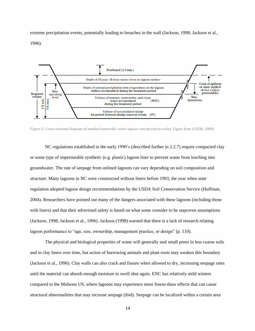
14
extreme precipitation events, potentially leading to breaches in the wall (Jackson, 1998; Jackson et al.,
1996).
Figure 3: Cross-sectional diagram of standard anaerobic waste lagoon concept (not to scale). Figure from (USDA, 2009).
NC regulations established in the early 1990’s (described further in 2.2.7) require compacted clay
or some type of impermeable synthetic (e.g. plastic) lagoon liner to prevent waste from leaching into
groundwater. The rate of seepage from unlined lagoons can vary depending on soil composition and
structure. Many lagoons in NC were constructed without liners before 1993, the year when state
regulation adopted lagoon design recommendations by the USDA Soil Conservation Service (Huffman,
2004). Researchers have pointed out many of the dangers associated with these lagoons (including those
with liners) and that their advertised safety is based on what some consider to be unproven assumptions
(Jackson, 1998; Jackson et al., 1996). Jackson (1998) warned that there is a lack of research relating
lagoon performance to “age, size, ownership, management practice, or design” (p. 110).
The physical and biological properties of waste will generally seal small pores in less coarse soils
and in clay liners over time, but action of burrowing animals and plant roots may weaken this boundary
(Jackson et al., 1996). Clay walls can also crack and fissure when allowed to dry, increasing seepage rates
until the material can absorb enough moisture to swell shut again. ENC has relatively mild winters
compared to the Midwest US, where lagoons may experience more freeze-thaw effects that can cause
structural abnormalities that may increase seepage (ibid). Seepage can be localized within a certain area

15
of a lagoon, and inspecting for such seepage is not easy; multiple groundwater testing wells at various
depths must be installed to monitor seepage properly (Jackson, 1998).
Huffman (1999) found that a sample of 36 swine waste lagoons constructed in ENC before 1993
did not pose a significant threat to groundwater off-site. This may suggest that efforts for monitoring
groundwater contamination may be better directed at the application of waste on sprayfields where
pollutants and pathogens are more likely to be mobile in rainwater runoff, or through tile drainage pipes
buried in fields (discussed at the end of section 2.2.3). Swine waste itself is not high in the nitrate ion
(NO3-) form of nitrogen (N), but the processes that convert other forms of N to nitrate increases when
waste is applied to soils. This rate depends on a variety of environmental conditions including climate,
pH, soil chemistry, and soil bacteria (Galaviz-villa, Martínez-dávila, & Pérez-vázquez, 2010).
Lagoons in ENC generally function to store diluted hog waste in an anaerobic environment. By
design, solids will settle to the lagoon bottom, and a minimum volume of liquid must remain above these
solids to help maintain anaerobic conditions. As new organic waste is added to the lagoon system, the
chemical and biological demand for oxygen (COD and BOD) remain high enough that virtually no
dissolved oxygen remains below the water surface, creating an environment where anaerobic microbial
processes dominate. A great diversity of bacteria in hog waste flourish in these lagoon environments.
Sometimes, additional bacterial cultures or chemicals are introduced to the lagoon to achieve more
desirable processing, such as for odor reduction.
Anaerobic bacterial processes differ significantly from aerobic processes. In anaerobic conditions,
large amounts of carbon are converted into methane gas (CH4, methanogenesis), and also a large
proportion of N is lost as ammonia gas (NH3, volatilization), both of which can escape into the
atmosphere and move off-site (Mikkelsen et al., 2000). The loss of waste materials from lagoons in
gaseous forms is not necessarily an unfortunate outcome for all farmers. To many farm managers with
very large operations, it is one of the benefits of anaerobic lagoon design, because it can lower the
absolute volume of waste that needs to be disposed of over time (Barker, 1996).

16
Losses of N content from waste can vary drastically depending on the exact methods of waste
management employed and environmental conditions. Approximately 20% of N from feed is assimilated
by industrial hogs, and 80% is excreted (Mikkelsen et al., 2000). Of the excreted portion of N, half is
released in urine and half in feces. Some waste management strategies separate these two waste fractions
and treat them in different ways to conserve nutrients and minimize nutrient losses, but in ENC they are
generally collected beneath the slatted barn floors, diluted, and flushed to the lagoon together. Up to 80%
of N from excreted material can be lost from the lagoon environment under poor conditions that promote
volatilization, and up to 40% of the N remaining in lagoon wastewater that is land-applied may be lost as
well (Jackson et al., 1996).
Over 40 different gases are released through anaerobic swine waste digestion by bacteria
(Mikkelsen et al., 2000). Besides ammonia and methane, the other two most common gases produced are
hydrogen sulfide (H2S), commonly known for its strong “rotten egg” smell, and carbon dioxide (CO2).
Dozens of other volatile compounds are also released, but in lower quantities. Hydrogen sulfide,
ammonia, and other volatile gases from swine waste can be irritating to human and animal respiratory
systems, eyes, and mucous membranes. Although ammonia and hydrogen sulfide are convenient to
measure, they “do not correlate well with human perception of odor” at off-site locations (Melvin et al.
1996, p. 56). The complexities in measuring and proving odor levels and odor transport distances make it
very difficult to use odor as a basis for emissions regulation. Many of the physiological irritations
experienced by workers and neighbors can be better traced to waste-dust particles, which can cause
allergic and inflammatory reactions, rather than toxic concentrations of gases (ibid).
Methane itself is odorless, but happens to be a powerful greenhouse gas. Methane is also
extremely flammable. For these reasons, a number of swine farms in ENC have been utilizing lagoon
covers that trap methane, and pipe it to systems that burn it to generate heat or electricity. These
technologies are still being developed and are not currently economically feasible for retrofitting the
thousands of old lagoons in ENC. However, as emerging carbon trade markets develop, swine farms
could be a potential source of carbon offsets that could make these technologies more approachable for

17
ENC producers (Upton, 2015). Methanogenesis is highly dependent on temperature; very little methane is
produced from anaerobic lagoons under 50 degrees Fahrenheit (Melvin et al., 1996).
In contrast to these anaerobic lagoons, most human (municipal) waste treatment is performed
with multi-stage systems with aerated ponds (Mikkelsen et al., 2000). The oxygenated environment
promotes aerobic bacterial digestion of waste, which minimize the release of odors, ammonia, and
methane. This is generally only possible by constantly pumping air (i.e. oxygen) into the system. This
technology is relatively expensive for swine farmers to install and operate, and has complications that
make it economically unfeasible for most swine producers at present.
Anaerobic lagoons are generally the cheapest and least complex of all treatment processes. In
some cases, the loss of nutrients and organic matter as gases is actually desirable if swine farmers value
dispersing large amounts of waste over the value of nutrients for fertilizer (Mikkelsen et al., 2000). Since
many states (including NC) currently require swine producers to have nutrient management plans
(NCDENR, 2009) that limit land application based on N needs for crops, the removal of N through
bacterial digestion in lagoons may allow more waste to be applied on less land. However, phosphorus (P)
can be over-applied to soil in these situations, as P generally remains in the solid fraction of waste.
Current regulations do also require the periodic testing of P in soils, which cannot receive waste
applications if concentrations exceed a certain rate (NCDENR, 2009). The addition of P as a more
stringent nutrient management limitation could have a significant impact on waste management in ENC.
Other macro- and micro-nutrients including potassium (K) zinc (Zn) and copper (Cu) may be building up
in many ENC soils that regularly receive swine waste (Mikkelsen, 1995). Cu and Zn are added to pig feed
to promote growth, but are utilized in only small amounts by crops (Jackson et al., 1996).
Lagoons are engineered to hold only a certain amount of waste (treatment volume) and liquid
(wastewater volume). Lagoon design will vary depending on the operation type, size, and the local soil
and topographic features of the site (Barker, 1996). Typically, sludge will build up on the bottom of a
lagoon over a period of years (Jackson et al., 1996). As sludge volume increases, less wastewater can be
stored in the lagoon. After a number of years, sludge will be removed, usually with dredging equipment.

18
Some farms agitate the sludge fraction and apply a higher amount of solid waste to their fields in order to
minimize this volume issue (USDA, 2009). Agitation can also increase the surface area of waste
accessible to bacterial decomposition within the lagoon, although this may increase odor issues. Dredging
of sludge must be done carefully and with proper equipment to avoid disturbing the lagoon lining.
Lagoon material must be applied to fields periodically in order to keep the lagoon volume below
a designed maximum operating level. This level is designed to allow one to two feet (0.3 to 0.6 meters) of
freeboard space between it and the top of the berm to account for extreme rainfall events that might cause
the lagoon to overflow. In most states lagoon freeboard is designed to withstand a certain extreme amount
of rainfall, usually the 25-year, 24-hour extreme rainfall event (Jackson et al., 1996). The estimated
amount of precipitation will vary depending on the climate of the region where the site is to be located. In
ENC, periods of extended or intense rainfall are not uncommon and can complicate a farm manager’s
ability to keep their lagoon within proper operating levels. Regulations in NC include restrictions on
applying waste to saturated fields or immediately preceding and during rainfall events (NCDENR, 2009).
Land Application of Waste: Nutrients vs. Pollution 2.2.3
In ENC, lagoon waste liquid is most commonly sprayed onto fields using fixed spray guns,
center-pivot irrigation, or travelling irrigation systems. Lagoon wastewater irrigation equipment does not
need to be significantly different from regular water irrigation systems, as long as only the liquid fraction
of the lagoon is being pumped. These irrigation methods are generally the cheapest for dispersing the
diluted waste from lagoons onto fields. In other regions, like the Midwest (with underground pit storage),
waste may be collected and stored with a much greater solid content. In these cases it is more appropriate
for waste to be injected into the ground (called knifing), which conserves nutrients and reduces odors.
However, injection requires expensive equipment and is labor intensive. Spraying diluted waste particles
through the air to reach across a wide field area increases the amount of waste that will float off-site,
increasing odor issues that can affect neighbors. Whether by accident or negligence, there are plenty of
cases where waste has been sprayed on nearby roads, on people’s homes, and into ditches and streams (a

19
Clean Water Act violation). Some swine farmers try to avoid applying in windy conditions, or will notify
their neighbors when they will be spraying so that people can prepare for the likelihood of unpleasant
outdoor conditions at those times. There are NC guidelines and regulations for appropriate conditions for
spraying, but data regarding actual application behavior of ENC hog farmers does not exist.
Figure 4: A fixed spray gun irrigates a field with lagoon wastewater in Warsaw, NC. Photograph by Don Young 2013,
permission of re-use granted by artist.
The greatest expense for fertilizing crops is N (Flanders, 2014), which, as discussed above, is
prone to volatilizing as ammonia gas, escaping from the soils and crops for which it was intended. When
swine waste is applied to fields, losses of N through volatilization of ammonia can be 40% or more, but
this varies significantly “depending on soil properties, environmental conditions, by-product
characteristics, and application methods” (Mikkelsen et al., 2000).

20
Since the mid-1900’s, inexpensive synthetic fertilizers have diminished the commercial value of
animal manure (Mikkelsen et al., 2000). The intensification of larger livestock production on smaller
amounts of land compounds the problem of waste management. Manure still has great value as a
fertilizer, but the nutrient focus is primarily on N, while often ignoring P, K, and other nutrients. The
market value of manure to be used locally, or to be sold commercially, is highly variable. Manure sales
depend on a number of factors: the ability of the farmer to prove the nutrient content, the local market for
manure or commercial fertilizer, the application methods available to the purchasing farmer, and the
timing of manure availability. Commercial chemical fertilizer is available at any time, but swine waste
“must be removed from lagoons on schedule, when the lagoon is full or before [which] may not coincide
with appropriate field conditions for application” (Jackson et al. 1996, p. 25). Manure is not a
homogenous material—the method of waste management used will greatly affect the nutrient and solid
content, and these contents will also vary over time. It can be difficult for a farmer to determine what the
exact nutrient content of their available waste material is, what the nutrient content will be when land
applied, and how much of that nutrient material will be plant-available in the soil during the growing
seasons.
N from lagoon material can be conserved by incorporating (tilling) it into the soil as soon as
possible after application, but this may only occur just before crops are planted. Many crops will not need
much N immediately when planted, but rather when they are maturing later in the season. Most N
volatilization will happen within one to three days of application, and at much greater rates if not
incorporated or injected into the soil. The general dilution of swine waste in ENC suggests that
incorporation of waste material by tilling will only occur when sludge is agitated or dredged, which will
occur less frequently than applications of lagoon liquid.
Since swine manure is applied to achieve only the N needs of crops in ENC, the ratio of N:P
should be of great concern. Swine waste often has an N:P ratio of 3:2, while some crops, such as corn,
have an N:P nutrient demand of 12:2. Thus, application of swine waste to meet N needs could mean
heavily over-applying P to the soil unless another concentrated N source is added (Jackson, 1998).

21
Jackson et al. (1996) echo the common concern regarding the increasing concentration of larger livestock
facilities in geographic areas and our lack of comprehensive understanding of the wider environmental
impacts from consistently over-applying nutrients:
“At some undefined loading rate, the local ecosystem can handle leakage, accidents, etc., but as
the loading rate increases, the ecosystem's capacity to absorb pollution without serious damage is
surpassed. This scale has not been determined in any systematic way for any region.” (p. 35)
There is much public concern for potential swine waste pollution of surfacewater and
groundwater from sprayfield activity. These concerns focuses mainly on nitrate (NO3-) loading and the
mobility of human pathogens into streams and shallow wells used for drinking water. P loading (in the
form of phosphates, PO43-
) is another concern, but it relates less directly to human health and more to
potential environmental impacts that affect water quality and aquatic wildlife. Aquatic recreation and
commercial fisheries are most directly impacted by N and P loading of streams that can lead to algal
blooms, eutrophication, and fish kills.
Nitrate is a relatively stable, water-soluble form of N, and its mobility through soil increases as its
concentration in the soil exceeds the level needed by plants. Unlike P, nitrate does not adhere to soil
particles. Public drinking wells (defined as a wells used by more than 25 people) are not commonly
contaminated and are tested often. Nitrate contamination is most likely to affect private, rural drinking
wells due to their proximity to septic leach fields, waste lagoons, or sprayfield locations (Drustrup, 2014).
These close proximities minimize the natural ability of soils and aquifers to attenuate (i.e. diminish) water
pollutants like nitrates, and pathogens. Since the setbacks of CAFO lagoons and sprayfields were not
regulated in NC until the mid-1990s, many rural wells might be vulnerable or affected. Rural NC
residents are encouraged to test their wells often for nitrates, nitrites, and fecal coliform bacteria at least
twice a year. Since 2008, new well constructions in NC are required to have an extensive water test
(CWFNC, 2015). Wells dug before 2008, however, may be untested, as it is up to the well owner.
Broadly alarmist perspectives regarding well contamination from (even unlined) waste lagoons in
ENC may not currently be supported by evidence (Huffman, 1999, 2004), but interest in further research

22
to assess the issue one way or another seems to have waned after the moratorium on new waste lagoons in
the late 1990’s (Rodney L. Huffman, personal communication, May 13, 2015). Huffman (1999, 2004)
and Jackson (1998) repeatedly echo the same calls as other scientists and concerned residents, for more
and better lagoon data from “field surveys of actual performance, over a range of climates and soil types
and a range of management and ownership systems” (Jackson, 1998, p. 115). Recently, Murphy-Brown is
facing new legal challenges after denying researchers access to swine farm sites to take groundwater
samples that they had previously agreed to during a 2006 legal challenge with environmental groups.
These groups alleged in 2006 that 11 Murpy-Brown swine facilities were violating the EPA’s Clean
Water Act (CWA) provisions (CWA discussed more in section 2.2.7), and must be evaluated by
researchers, yet these studies have not been allowed to proceed (Raposo, 2015).
Over-application of N and P can be an issue with swine waste management because nutrient
content within—and between—waste applications is heterogeneous. It is also difficult to evenly distribute
animal waste to hundreds of acres of crop fields. Wastewater saturation of fields is not uncommon, and
can occur from faulty equipment or by accidents, such as if a farmer simply forgets to turn off a pump, or
from improper application directly preceding, during, or after significant precipitation events (Jackson,
1998). More nefarious discharging directly to ditches, streams, or anywhere other than crop fields at
agronomic rates is an illegal behavior, but has been documented time and again, mostly by industry
watchdog groups and neighbors. Niman (2008) describes years of accumulated violations evidence in her
accounts of legally representing the Waterkeeper Alliance, a national environmental group that brought
charges against corporate animal producers in the early 2000s under the CWA.
Despite what some industry opponents suggest, there is insufficient evidence to support a claim
that pumping waste directly into ditches and streams is a general behavior of hog farmers. It is, however,
true that the burden of bringing such illegal instances of discharges to light is on the shoulders of citizens,
rather than state inspectors, who are understaffed in many states due to a lack of funding for inspector
positions (Genoways, 2014; Jackson et al., 1996; Niman, 2008).

23
Concerns for human health impacts from sprayfield activity include the potential transport of
human pathogens. About 50% of all bacteria and 90% of viruses can be expected to be eliminated during
anaerobic digestion in the lagoon (Jackson, 1998). Still, the initial concentration of pathogens is so high
that even these losses do not eliminate the potential danger of contamination. When transported by water
through soil and groundwater pathways, the survival of pathogens is determined by a variety of factors.
Temperatures and the amount of infiltrating water (i.e. climate), soil/aquifer characteristics (e.g. physical
structure, biochemical soil-water interactions), and the type of pathogen, can all affect survival of a
pathogen as it moves through groundwater pathways (ibid). Antibiotics, antibiotic resistant bacteria, and
pathogen transmission between CAFO laborers and hogs will be discussed more in the section on
antibiotics and disease (2.2.5). It is plausible for human pathogens to survive transportation in field runoff
from precipitation events, from waste spills, or (even more likely) through tile drains installed in fields
that output directly into ditches that inevitably lead to streams.
Tile drains in ENC are a common pathway for saturated sprayfields to leach abnormal amounts of
nutrients into ditch networks that ultimately reach public surface waters. O’Driscoll (2012) estimates that
over 2 million hectares (five million acres) of drained agricultural lands exist in North Carolina, with the
majority in the Coastal Plain. Tile drains are often necessary to keep fields in this region from becoming
waterlogged. They are essentially perforated pipes buried into the ground at a certain depth below the
level of plant water uptake. They help convey the water that saturates soil at this depth, moving it out of
the fields and into ditches. This enables more rapid percolation of water through the upper layer of soil in
periods of extended or extreme precipitation. In other words, tile drains and ditches lower the water table
locally (ibid). O’Driscoll (2012) mentions a number of studies that demonstrate how subsurface drainage
can actually lower P contributions from fields by decreasing surface runoff (i.e. decrease losses of
sediment which P adheres to); however, this can also cause large increases in N export compared to
surface drainage (pp. 66-68).
Harden and Spruill (2004) showed that, of 18 tile-drained fields receiving either commercial
fertilizer, swine lagoon effluent, or wastewater-treatment plant sludge, the swine effluent sprayfields had

24
significantly higher median annual nitrate loading—15 times greater than fields receiving commercial
fertilizer. Even though drainage tiles are technically point-sources of pollution, they are considered non-
point-sources for agricultural purposes under the CWA. This exception may soon be challenged in court,
as discussed in section 2.2.7 regarding externalities.
Life Stage Segmentation and Feeding 2.2.4
Raising hogs separately based on their stage of life is an important part of the industrial model of
pork production. In order to streamline building requirements, caretaking needs, and feed components, it
is most efficient to separate industrial hog operations into a few life stages. The housing of sows
(reproducing female pigs), artificial insemination, gestation, birth, and raising the piglets on the sow’s
milk for two to three weeks is all part of a process known as farrowing. The gestation period of sows is
about 115 days, or almost 4 months. There are around 8 to 12 pigs born in each litter, and they feed on the
sow’s milk for a few weeks. Piglets are separated from their mother when they are around 10 pounds,
becoming “weaned” pigs. Weaned pigs are raised until around 60 pounds, and are thereafter called
“feeder” pigs. The wean-to-feeder period is sometimes also referred to as the “nursery” phase. The
operations that continue raising feeder pigs until slaughter weight, around 250 pounds, are known as
“finishing” operations.
In terms of number of permitted operations, feeder-to-finish is the most common in NC (56.3%),
followed by wean-to-feeder (21.7%), and farrow-to-wean (14.5%) (Figure 1). A smaller number of
operations raise pigs from farrow-to-feeder (2.2%) and wean-to-finish (1.9%). Some operations still do
perform the entire process of raising pigs, known as farrow-to-finish (1.5%).

25
Figure 5: Number of permitted NC swine operations by type in 2015 (NCDWR, 2015)
It is often more appropriate to discuss operations in terms of the estimated steady state live weight
(SSLW) instead of the head count. SSLW is the average weight of animals at an operation over the course
of a year. This is calculated by multiplying the permitted operation head count by a static formula value
depending on the type of operation. This is especially relevant when discussing farrowing operations,
since the average piglet head count is not included in “allowable” head count totals. Instead, the SSLW
incorporates the expected weight of the sow and a litter of piglets that are raised to the size of that specific
operation type (e.g. wean, feeder, or finishing pigs). For example, each sow counted at a farrow-to-wean
operation will be attributed a considerably smaller estimated SSLW than a sow at a farrow-to-finish
operation.
Farrowing operations are larger and more complex than feeder or finishing operations. In terms of
infrastructure, the buildings that house sows are generally larger and more numerous than in finishing
operations, and more varied in shape and in site layout. Farrowing operations also require a greater range
of worker skills and more attention in terms of handling, feeding, and medical care. Sows grow to be
much larger than slaughter weight of finishing pigs; sows commonly reach over 500 lbs. In the US
1308
505
336
51 43 36 28 17 0
200
400
600
800
1000
1200
1400
Feeder toFinish
Wean toFeeder
Farrow toWean
Farrow toFeeder
Wean toFinish
Farrow toFinish
Gilts Boar/Stud
Nu
mb
er
of
Pe
rmit
s
Type of Operation
Number of Permitted NC Swine Operations by Type (2015)

26
industry, sows are generally bred for about three years, until they lose optimum litter production and are
sold for slaughter.
In NC, it is common practice to use gestation crates to hold sows in small individual pens where
they will not interact with other sows while gestating. Sows—and hogs in general—create a social
hierarchy among themselves, which can be problematic when sows establish dominance. Aggressors can
keep others from getting the amount of feed intended for them, and physical abuse among sows can occur
in group pens. Sows are often feed-limited, rather than being allowed to eat as much possible as in feeder
and finishing operations. The measure of control allowed by gestation crates—while convenient for
individual observation, feeding, and medical care by the farmer—is increasingly being attacked by animal
welfare groups because the sows are given such little room in these crates that they cannot roll over, turn
around, or socialize for months on end. Groups like the People for the Ethical Treatment of Animals
(PETA) and the Humane Society of the United States (HSUS) have successfully led campaigns in some
states to have the practice banned entirely. Large corporations like Walmart and McDonalds are
increasingly requesting the elimination of gestation crates from their pork sources (Strom, 2015). Even
Smithfield itself, one of the largest pork corporations in the world, is trying to get its contracted growers
to phase out gestation crates (Doering, 2014). Major production regions like Iowa and NC are not
currently debating legislation on this matter. In these states, gestation crate reform would likely have a
very strong economic impact on the farrowing sector of the industry.
Less controversial, but similar, is the use of farrowing crates. These are used during and after the
birth of a litter to limit the movement of the sow while piglets are in the suckling phase. It is a common
occurrence for sows in confined situations to negligently roll over and crush their piglets to death, but the
farrowing crates help minimize this occurrence. Other actions taken during the farrowing phase is the
docking of tails, clipping of sharp teeth, and castration of male piglets.
In pork production, male pigs that go through puberty and become boars are generally more
aggressive than their castrated counterparts, known as barrow pigs. Boars also give off a strong,
undesirable odor that will persist in the processed meat after slaughter. Compared to sows and finishing

27
pigs, there are very few boars that are kept for production of semen to breed market pigs. These are called
boar/stud operations. Collection and insemination is performed manually by workers. Feeding and
finishing are relatively the most straightforward operations, requiring less capital investment in
infrastructure compared to farrowing operations.
Swine feed is a major industry in and of itself, and the subject of much agricultural science
research at land grant universities in the US and agri-science companies across the world. Everything
from nutrient content to particle size is scrutinized and assessed at all growth stages and for all variables
of swine operations. Here a brief overview of feed type and geographic source should suffice for this
study. The major types of hog feed in industrial operations are corn and soy, and these feeds constitute the
primary operational cost of swine operations. Significant amounts of corn and soy are grown by NC
farmers, but sheer demand to feed millions of pigs necessitates that most will be imported, often from the
Midwestern states where it is produced in greater amounts and sold more cheaply.
Other feed input materials are combined with corn and soy to produced tailored diets depending
on the life stage, and are targeted to meet the specific local needs of a producer. Feed components can be
customized to some degree to minimize the excretion of nutrients like P and other molecules like copper.
Certain physical properties, like using pellets instead of meal, have been shown to significantly reduce
feed wastage. Highly selective pig genetics and the nurturing of optimal bacterial flora in the gut are also
important aspects determining how feed will be digested by the pigs.
Like all aspects of agriculture and livestock production, economics plays a major role in inputs
and management strategies employed at an operation. Not all farmers will be able to pay for the cutting
edge of odor-reducing and nutrient-conserving feed formulas. Often a contracting producer will have feed
provided for him by the contract corporation. In regards to the general hog operations, the price of live pig
sales are invariably tied to fluctuations in feed markets. Certain global or regional market swings can have
drastic effects on hog farmers, such as in 2005 when the EPA created its Renewable Fuel Standard, which
“required 7.5 billion gallons of renewable transportation fuel within seven years” (Genoways 2014, p.
214). This ironically creating a corn-planting frenzy to reap the benefits of quadrupled ethanol prices,
28
causing a corn feed market disaster and driving up pork production costs. Because of the notoriously tiny
margins of profit that hog farmers sustain their livelihoods on, the fluctuations in feed prices can mean the
difference between a bumper year and selling the farm if they do not have a contract with a major
corporation.
Anti-biotics, Disease, Mortality, and Disposal 2.2.5
The proper medical care of livestock is a necessity in any kind of husbandry. However, the rate of
medical applications of antibiotics to swine in CAFO environments is high, as disease can spread easily
and quickly through a population in such confined conditions. Disease can be devastating for individual
swine producers, but the spread of infection from a single farm can also become a major concern for the
industry on a regional, national, and even international scale. It is not uncommon for nations to entirely
ban the import of live animals or certain kinds of processed meat from other areas of the world that pose a
risk of disease transmission to their country.
In 2013, ENC experienced a particularly devastating blow to its pork herd when outbreaks of
porcine epidemic diarrhea virus (PEDv) wiped out nearly 1/3 of the piglets in the state (Fernandez, 2015).
Nationally, more than 10 percent of the U.S. herd was destroyed. PEDv is a highly transmissible, and
deadly to piglets, although not as dangerous for older pigs. It is still not confirmed how the virus entered
the country, but outbreaks began in April 2013. The PEDv epidemic revealed important biosecurity issues
in the U.S. pork industry that led to widespread behavioral changes on individual farms and for the
transportation and feed industries as well. Another disease outbreak is inevitable, but the industry is
turning its lessons learned from PEDv into increased preparation and coordination for the next potential
epidemic.
In addition to improving biosecurity, the swine industry in the US is also reforming its usage of
drugs in animal feed under the Veterinary Feed Directive (VFD), which comes into effect in 2016
(USFDA, 2015). The VFD essentially creates a regulatory framework for antibiotic drug applications to
livestock through feed. Producers may only use drugs in animal feeds that are FDA approved, and only

29
when approved as medically necessary by a licensed veterinarian. One might wonder why this directive is
necessary—why are producers applying antibiotics to their animals through their feed when it is not
medically necessary? The answer is surprising, and may have important implications for human health.
Ted Genoways (2014) reviewed the history of this practice of applying antibiotics to animal feed.
The story begins in 1945 when the antibiotic drug aureomycin (chlortetracycline) was discovered in 1945
by a botanist, Dr. Benjamin Dugger. Dugger wanted to understand why chickens who were able to peck
through manure for bugs “experience lower mortality rates and higher egg production than pullets raised
in ‘cleaner’ environments” (p. 198). Dugger found a certain fungus in manure-fed soils that had very
special properties—it was effective at combatting 90% of common bacterial infections in humans. It also
had an interesting side effect of causing patients to put on weight. Around 1950, animal tests concluded
that adding aureomycin to the diet of weaned piglets and baby chickens could almost double their feed
efficiency. This dual benefit of promoting growth and preventing disease was one of the foundations of
the broiler chicken CAFO industry. Scientists also found that extended dosages to swine did not actually
eliminate undesired pathogens from the gut of hogs. Rather, consistent, non-medical doses of antibiotics
contributed to the breeding of antibiotic-resistant pathogens.
Antibiotic-resistant pathogens are increasingly recognized as potential health threats to humans.
One major concern today is methicillin-resistant Staphylococcus aureus (MRSA) associated with
livestock and also multidrug-resistant strains (MDRSA), which “have made treatment of S.
aureus infections more protracted, more burdensome, and less successful” (Rinsky et al., 2013). Pig-
associated strains of MRSA seem to be the strongest evidence to support the argument that over-
application of livestock antibiotics could eventually impact humans (McKenna, 2013).
Mortality of pigs can occur at any stage of life. Most losses are “routine,” but others, such as the
PEDv epidemic mentioned above, can sometimes be “catastrophic” (Harper, DeRouchey, Glanville,
Meeker, & Straw, 2008). Other catastrophic losses may occur from barn fires, ventilation equipment
failures, or hurricanes and floods. In general, the great concentration of hog farming in ENC ought to
necessitate some organized and regulated manner of carcass disposal that prevents odor nuisances and
30
potential environmental contamination or human health impacts from the decaying animals. There is in
fact no “best” disposal method, as different methods have their relative benefits and problems depending
on the situation and locale.
Some areas employ regional rendering facilities that subject carcasses to intense heat to eliminate
pathogens, and may also utilize some kind of chemical pre-treatment. The output rendered material may
be used as a protein source in certain kinds of animal feed. There are costs associated with transporting
the dead animals, and there are also biosecurity risks to farms from disease-exposed transport trucks.
Some hog farms in ENC use “dead boxes,” which are essentially steel waste containers placed on the
edge of a farm property where dead pigs are dumped. The carcasses are then scheduled to be picked up
and transported to rendering facilities so that the trucks never have to enter the farm premises.
Other routine disposal methods include simple burial, incineration, or a more involved process of
composting. Because of increasing regulation of rendering facilities, some regions are finding it too costly
to support this disposal option. In ENC the most common alternative to rendering—on-site burial—is a
concern because of the high water tables and permeable sandy soils, which increase the risk of
groundwater contamination. During the ongoing PEDv outbreaks in 2014, the Waterkeeper Alliance (a
national environmental watchdog organization) published a letter asking NC Agriculture Commissioner
Steve Troxler about how hundreds of thousands of dead pigs were being disposed of during the crisis
(Waterkeeper Alliance, 2014). Troxler’s response indicated that his office was confident in the current
methods of rending and composting as adequate disposal options for the situation (Strom, 2014), but the
Director of Livestock Health, Dr. Tom Ray, offered conflicting information—that on-site burial was the
most common method of disposal during the situation.
The size of the piglets killed by PEDv are very small compared to finisher pigs or sows. The
smaller size of the piglets makes composting a more viable method than for the larger pigs, and transport
of piglets off-site for rendering may have been undesirable due to the increased potential to spread the
disease. State regulations in NC require burial of pigs at least two feet (0.6 meters) underground or
transported to a rendering plant within 12 hours (NC General Statues 106-310 and 106-319), but do not at

31
all address the issue of catastrophic disposals or the potential contamination of groundwater in some
places with a relative high water table. This lack of clear public information during such an emergency
does not lend well to general confidence in the state’s preparation for a potential catastrophic loss of
livestock from flooding or a different sort of epidemic. After Hurricane Floyd, there was a lack of
coordinated effort for livestock disposal, and farmers ended up burying hundreds of dead animals in mass
graves on-site. Iowa, the largest hog-producing state, appears to be more prepared by having “a set of
disposal methods for use during emergency disease outbreaks. They range from burial and rendering to
use of alkaline hydrolysis, a highly specialized process using chemicals and heat to break down tissues”
(Strom, 2014).
Processing Facilities, Vertical Integration, and (Some) Resistance 2.2.6
The Midwestern US states have traditionally been home to the vast majority of the nation’s pork
production and processing for well over one hundred years. This has been due, in large part, to the
regional production of plentiful amounts of cheap corn, which serves as the foundation for the Midwest
herd. There is a saying that a pig is “20 bushels of corn on four legs,” and this harkens back to a pre-
railroad era when large herds of hogs actually had to be walked, sometimes hundreds of miles, to distant
markets for sale and slaughter (Essig, 2015, pp. 153-165). Instead of exporting all of the bountiful
amounts of excess corn grown in the Corn Belt and other rural states, it was often exported it in the
concentrated and value-added form of pork instead.
Pigs can conveniently transport themselves, or their butchered meat can be salted and cured to
last several months before perishing. Pork is highly amenable to a variety of curing processes (unlike beef
and poultry) and thus was the most transportable meat before refrigeration cars were available. Pork was
eaten more by Americans per pound than any other meat until the 1960s, when beef eclipsed it on the
American dining table. As railroad networks developed in the late 1800s, slaughtering facilities became
larger and more industrialized, and pork processing became more centralized in urban railroad hub cities
like Cleveland, and later Chicago.
32
The Chicago meatpacking industry was made infamous from its (accurate) depiction by Upton
Sinclair in his 1906 novel, The Jungle. Sinclair’s fiction functioned more like an exposé on the deplorable
conditions of meatpacking workers and virtually non-existent food safety measures and oversight for
slaughtering, processing, rendering, and the ultimate destinations of less desirable animal byproducts.
Still today, animal processing facilities are not totally cured of food and worker safety violations.
Periodically, a high-profile scandal brings down a processing plant or ruins an entire company
(Genoways, 2014).
Scandals aside, the processing aspect of the industry is obviously an integral part of the global
meat market. From a certain perspective it is a marvel of industrial efficiency. As Sinclair (1906) wrote,
“they use everything about the hog except the squeal.” Indeed, all parts of a hog are turned into some
useful product or commodity. Besides meat and some organs destined for human consumption, various
other pig parts go on to become medicines (e.g. insulin and blood thinners), hair brushes (made from
bristly hog hairs), gelatin, and a great miscellany of industrial products like pet food, biofuels, cosmetics,
and crayons (Lowe, 2014).
The spatial and economic structures of the animal processing industry have changed in significant
ways since the middle of the 20th century. There has been an overall shift away from centralized urban
hubs like Chicago to more rural locations where cheap labor is plentiful, yet regional access to urban
markets is still strong. In some cases, labor is being imported into these rural areas from outside of the
US, causing conflicts to arise between local communities and the processing companies (Genoways,
2014; Grey, 1998). At the same time, working conditions may be harsh for these immigrant workers
because they do not have the same legal recourse as citizens; overworking and on-the-job injuries may
leave them permanently disabled and yet unable to receive compensation (ibid).
Consolidation of the industry is an important part of the story explaining why ENC became such
a powerful component of the national and global pork business. Pork businesses in general have become
highly consolidated after decades of mergers and acquisitions since the 1970’s. Large meat processors
eventually integrated the various business aspects of feed milling, genetics and breeding, and hog

33
production as well, such that a single corporation and its subsidiary companies may own and operate the
entire pork product chain from seed to marketed bacon. In North Carolina, Smithfield Foods became the
primary integrator, owning and contracting with hundreds of hog farms while also operating the major
pork processing facilities in the state. Murphy-Brown is current the hog production subsidiary company
of Smithfield Foods, and is itself a combination of a number of formerly-independent hog production
companies like Murphy Family Farms, Browns, and Carroll’s Foods. A wholly separate company,
Maxwell Foods, remains a significant hog producer in NC that partners with Smithfield for certain
dealings and also operates its own meat processing enterprises out of state. Prestage Farms is a separate
corporation with significant pork production in NC. Prestage partners with Smithfield, but also produces
poultry and operates their own processing enterprises out of state as well.
Before integration, independent hog producers used to bring their hogs to a variety of auction
houses, like chicken farmers before poultry integration (Morrison, 1998). As integration (i.e. contracting)
eliminated the need for the traditional auction houses, and as the smaller slaughterhouses were bought out
or closed due to competition, independent hog farmers found that their smaller volumes of pigs lost their
level playing field in the market (ibid). Meanwhile, corporate integrators became more resilient to
common four-year pork supply cycles and feed market fluctuations through long-term contracts on both
the supply and demand sides of the business. Smithfield made a strong pivot into North Carolina in the
early 1990’s, opening the largest slaughtering facility in the world in ENC in 1992, and gaining control of
other major processing facilities in the area (discussed more in section 2.3.7). The economies of scale and
streamlined efficiencies of integration steadily drove down the price of pork and further increased farm
loss, mergers, and integration.
The substitution of labor by large capital investments in mass-production technologies (i.e.
automation), and a shift to centralized corporate management of standardized facilities, is one of the
primary economic advantages of corporate integration and contracting (Ikerd, 1998). However, research
suggests that larger hog operations are less supportive of local communities (ibid). That is, the rate of

34
local spending by farm workers and owners of larger facilities is significantly less than workers from
smaller or moderate-sized operations.
Although this will not be discussed in depth here, the economic and social losses to local
agricultural communities from industrial hog farm restructuring is one of the major criticisms of the
increasingly integrated hog industry. However, valuating or otherwise quantifying net losses or gains to
rural communities has proven to be a challenge for researchers. Industry proponents remain adamant that
corporate contracting is saving or creating many farmer livelihoods and supplying steady incomes to
economically-depressed rural communities. Opponents suggest that farming communities have suffered
net losses in income due to the automation enabled by capital-intensive hog farm technologies. Decreased
property values due to hog farm odor nuisances can impact individuals and neighborhoods financially, but
the deterioration of one’s mood and quality of life is harder to quantify. Further, rural communities have
suffered adverse impacts in social dimensions that defy valuation (K. M. Thu & Durrenberger, 1994).
In the last 20 years, E. Paul Durrenberger and Kendall M. Thu (professors at the University of
Iowa) have been two of the most outspoken academic voices calling attention to the deteriorating
conditions of rural family communities in Iowa from industrial agriculture. Their work in the mid-1990s
presciently referenced North Carolina as the “future Iowa” in terms of the hog farming landscape.
Although the NC industry was admired for a number of innovations, their description of rural conflicts
due to industrial hog farming did not paint a rosy picture. Durrenberger and Thu repeatedly encountered
evidence of “widespread intimidation and the erosion of democratic political processes” (Durrenberger &
Thu, 1996, pp. 20-21). They go on to describe findings that the “pathological interlinkages between swine
industry interests and political office” (ibid) erode the power of regulation and retard the normal avenues
of citizen redress in the courts or to county and state officials (NC-specific legislation is discussed more
in section 2.3.7). Intimidation and institutional pressure to prevent industry criticism was a theme brought
up numerous times in personal communication with researchers during this study.
Opposition to corporate ownership or control of agricultural production is not an emergent
position of locally impacted communities or environmental organizations in recent years. This position

35
has been held by every state that makes up the traditional agricultural heartland of America for most of a
century. During and after the Great Depression, the Great Plains states created laws that forbade or
restricted publicly-owned corporations from owning certain agricultural operations, in order to “preserve
and protect the family farm as the basic unit of production” (Krause, 1983, p.41, as cited by Schroeter,
Azzam, & Aiken, 2006, p. 1000).
North Dakota was the first state to create anti-corporate agriculture laws in 1932. Nebraska was
the most recent state to pass such legislation, in 1982. In the 50 years between, Iowa, Kansas, Minnesota,
Missouri, South Dakota, Oklahoma, and Wisconsin have all passed anti-corporate farming legislation,
although the details and degree of restrictions vary. In the last 30 years, however, these laws have
increasingly been scaled back or dismantled after years of court battles and costly campaigns to sway
public opinion one way or another. Critics of these laws mainly hold that farm viability and competition
in modern agricultural markets demands significantly more capital investment and greater economies of
scale than can generally be achieved from individual family farmers or even incorporations of farmers.
Thus, many critics argue, these laws effectively restrict state-wide agriculture from adjusting output to
meet the increasing global demand for animal products.
As Smithfield Foods is the largest individual processor of pork in the world, it is interesting to
note that the Chinese meat processing company Shuanghui International (now called the WH Group)
bought Smithfield for $7 billion dollars in September 2013. This was the largest acquisition of an
American company by China to date (Palmer, 2013). The deal was so big, and had such important
economic implications for the U.S. food market, that it was considered a potential issue of national
security and was brought up for review by the Committee on Foreign Investment in the United States.

36
Figure 6:The top 10 pork-producing countries as of 2013. Graphics sourced from the US Pork Checkoff’s 2014 Pork Quick Facts
(US Pork Checkoff, 2014).
China leads the world in total national annual pork production at 55.6 million metric tons
compared to 22.4 in the European Union and 10.5 in the U.S. as of 2013 (Figure 6), but regions of the
E.U. and the U.S. generally have a greater production density. As China's population and median income
rises, its burgeoning middle class increasingly demands meat; pork is by far the most popular. Hogs in
China have traditionally been distributed across small farms all over the country with only a few head
each (Pig International, 2005). China may be reaching the maximum production capacity for their current
decentralized small farm paradigm, and if they do not switch to more intensive production (i.e. CAFOs)
they will necessarily need to be importing more and more pork in the coming years (Neo & Chen, 2009).
Smithfield's acquisition by China may be seen as a foreshadowing of more acquisitions of international
pork to feed its growing demand in the future. Most recently, China stands to import 45 percent more
pork in 2015 than the previous year as it has culled close to 100 million hogs and 10 million sows since
2014 (Singh, 2015). This loss is equivalent to the standing herds of the U.S., Mexico, and Canada
combined. It is worth wondering, if Chinese and other international demands for pork continue, might the
economic and political climate in North Carolina shift enough to press for a new wave of pork expansion?

37
Defining and Addressing Externalities 2.2.7
In economics, an externality is defined as something that happens when a person (or business
entity) engages in an activity that “influences the well-being of a bystander and yet neither pays nor
receives any compensation for that effect” (Mankiw 2008, p. 204). An adverse impact is called a negative
externality. Some degree of negative externality may exist for nearly any productive human activity, but
certain industries have more acute or measurable impacts than others. Environmental monitoring,
research, and cleanup efforts for many industries are paid for by public tax dollars in the absence of strict
regulations or targeted taxing strategies. Some industries have been regulated to different degrees by
government in order to protect human well-being, or to conserve environmental resources. Or, on the
other hand, regulation can be used to protect industry from what some might consider overzealous
environmentalism or NIMBY (Not in My Back Yard) cases. These kinds of protections for industrial
agriculture are evident in the current “Right to Farm” laws in many states, including NC.
Positive externalities can also arise from industry, and are not mutually exclusive with negative
externalities. This may occur when the creation of economic opportunities for struggling communities or
regions also benefits those who do not work directly with the industry by raising overall wealth and
spurring economic activity in an area. As discussed briefly in the previous section, some potentially
impacted facets of rural community life, such as social dimensions, may be impossible or inappropriate to
valuate in quantitative or financial terms (K. M. Thu & Durrenberger, 1994).
This study would be remiss without some introduction and discussion of the Clean Water Act,
which is one of the foundations of federal and state regulatory framework that addresses negative
externalities of industry. The Federal Water Pollution Control Act of 1948 was the first major law passed
in the U.S. to generally address pollution of the nation’s water resources. In 1972, increasing public
awareness of water pollution issues and the need to control them led to “sweeping amendments” to the
1948 law, which afterwards became known as the Clean Water Act (CWA). The CWA had numerous
goals to “restore and maintain the chemical, physical, and biological integrity of the Nation’s waters, with
interim goals that all waters be fishable and swimmable where possible” (U.S. EPA, 2012).

38
Authority for establishing limits, objectives, and guidelines was vested in the Environmental
Protection Agency (EPA, established in 1970 under President Nixon), but the CWA embodied a new
federal-state partnership, where “states, territories and authorized tribes would largely administer and
enforce the CWA programs, with significant federal technical and financial assistance” (U.S. EPA, 2012).
Under the CWA, all pollution discharges (pollutants defined by the EPA) to the nation’s waters are
unlawful unless authorized by a permit. The CWA primarily had a technology-based approach focused on
limiting pollution from industrial and municipal point-sources, such as factories and water treatment
facilities.
Defined water quality standards are the foundation for the CWA water protection programs.
Specific water quality targets were developed by states and tribes with support and review from the EPA.
All states review surface water conditions every two years to maintain lists of “impaired waters,” which
are water bodies that do not meet targeted water quality standards. The CWA requires states to address
impaired waters by developing water restoration plans, which include establishing total maximum daily
loads (TMDLs) of pollutants. TMDLs serve as an allowed pollutant “budget” for all upstream discharging
activity.
Any facility that may be a point-source discharge of a pollutant (e.g. from pipes, ditches, or
gutters) must obtain a National Pollutant Discharge Elimination System (NPDES) permit. These permits
define a facility’s allowable amount of discharged pollutants (in context of the relevant water body’s
TMDL) to achieve the target water quality standards. Most NPDES permit are administered at the state
level, and point-source facilities (including municipal stormwater and wastewater treatment facilities)
must show that they are using the “best available technology to reduce pollutants from their discharges”
(U.S. EPA, 2012). Violations of the NPDES permit terms may invite significant penalties. The CWA
enables citizen suits to be filed against violators of NPDES permits, or against the “EPA Administrator’s
office (or equivalent state official) for failure to carry out their duties as specified under the CWA” (ibid).
In 1987, CWA was expanded to develop programs to control nonpoint (diffuse) sources of
pollution as well, including pollution from agricultural activity. The US EPA’s National Estuary Program
39
(NEP) was also established through a CWA amendment that year. The NEP provides grants to research
and assess threats to the 28 estuaries of national significance. One of these NEP sites is the Albemarle-
Pamlico Estuary System (APES) in ENC, one of the largest estuaries in the nation (section 3.4 discusses
physical geography of ENC). Assessment and conservation efforts for the APES are coordinated through
the Albemarle Pamlico National Estuary Partnership (APNEP), funded through the NEP. CWA
amendments and programs over the years have evolved towards a more “integrated, place-based
watershed protection strategy” (U.S. EPA, 2012). This attempts to concurrently address a host of
interrelated issues by involving multiple stakeholders at the state and local level; together, they develop
and implement strategies to achieve and maintain state water quality goals (and additional environmental
goals).
Although many large swine CAFOs in ENC fell under the CWA’s standard definition of a CAFO
requiring an NPDES permit after 1987, important details in the wording of the CAFO definition
exempted most swine farms. The federal standards stated a CAFO was a facility with 2,500 or more
swine each weighing less than 25 kilograms, or 750 swine each weighing over 25 kilograms; and, where
“pollutants are discharged directly into navigable waters through a manmade ditch, flushing system, or
similar device” (Burns, 1996, p. 867). The definition above gave exception to swine farms because they
were constructed, in theory, to hold all waste on site and only apply it to agricultural fields (considered
normal agricultural activity, like fertilizer); waste is never intended to be conveyed into streams from any
point source. Despite meeting the numerical requirements of the defined CAFO size, the swine farms
were exempt from permitting as long as their lagoons were engineered to withstand extreme precipitation,
up to the federal standard threshold of a 25-year, 24-hour storm event (i.e. an estimated 4% annual chance
of recurrence).
In 1995, 1996, and 1997, the NC congress passed sweeping reforms of hog farm oversight which
finally implemented permitting, inspections, and siting restrictions for new hog farming operations,
among many other changes. NC-specific legislation regarding hog farming will be discussed further in
section 2.3.7 and 2.3.8. On the national scale, the reach of the CWA has been challenged—and will

40
continue to be challenged—by the livestock industries and its opponents to scale back or expand
restrictions placed upon CAFOs. Industry compliance with regulations and government capacity to
enforce violations are significant hurdles to actually achieving many regulatory goals (e.g. industry’s
internalization of costs from adverse impacts). CWA court cases demonstrate that the Act’s seemingly
simple and precise language—“any discharge of pollutants into navigable waters of the United States is
unlawful unless the discharge is made pursuant to an NPDES permit”—in reality has been a “complex
and largely uncharted labyrinthine statute” for many agricultural applications, which have to be waded
through in extensible court cases over time (Todd, 1996, p. 500). Periodically, the EPA amends the CWA
to clarify its language, or to address legal findings from court cases (sometimes after the EPA itself is
sued by agricultural or environmental organizations). Most recently, in August 2015, the EPA released
the Clean Water Rule, a 297-page document meant to clarify what the phrase “waters of the U.S.” means
in the CWA language, among other things. The EPA emphasized that these additions to the CWA would
not affect agriculture, however, “a long list of state and local governments, businesses and agriculture
organizations did not see this rule change as crystal clear, but rather as a mucky mess” (Day, 2015).
State and federal policies and regulatory decisions are based on certain scientific epistemologies
and ontological assumptions about what is “healthy” for human beings, and what the “natural”
environment is and how we should manage it sustainably. Likewise, environmental or social interest
groups have their own set of understandings and relative priorities for human well-being and
environmental protections, often in conflict with economic and political interests. Each perspective is
informed by a selected body of scientific knowledge, theoretical perspectives, and ethical or moral
components of “justice” and “rights.” These perspectives can change over time, as does the language and
meaning in the discourse used among them (e.g. the use and meaning of the term “family farm”). The
espoused perspectives of government agencies or administrators, industry lobbies, or other interest
groups, can all be entangled in additional short-term political motivations and complexities beyond a
specific regulatory issue at hand.

41
Due to the vast complexity of ecosystems and the limited funding provided for research, Jackson
(1996) suggests that “…currently, ecosystems are being ‘managed’ by default, by a social, political, and
economic system which is largely unaware of ecosystem constraints or consequences” (p. 39). In the 20
years since Jackson wrote those words, some areas, like Iowa, have been experiencing increasing negative
externalities from industrial agriculture. There remains an ongoing debate about what level of
environmental pollution is safe and acceptable, and what role government should or should not have in
regulating agricultural activity.
A recent illustration of a response to externalities from industrial agricultural can be seen in the
legal action being brought by the Des Moines Water Works (DMWW) against three counties in
Northwest Iowa that are upstream of it, in the headwaters of the North Raccoon River. The DMWW
provides water to the 500,000 residents of Des Moines, in central Iowa. Ted Genoways (2014) describes
the perspective of the DMWW and the basis for their lawsuit:
“[Scientists at the DMWW] have been tracking steady increases in levels of nitrates and E. coli in
the contributing watersheds since the 1970’s, when industrial agriculture first started to hit its
stride. But in the last decade [2004 to 2014] those levels have started to assume a predictable
pattern: spikes track with periods of peak manure application with noticeable increases each
November and then vertiginous leaps to dangerously high concentrations in late spring and early
summer. And in the past decade those nitrate levels have started to pose greater and greater
threats to public health—an even broader source of concern than the spread of antibiotic-resistant
bacteria.” (p. 225)
In 1991, the DMWW built an ion exchange nitrate-removal plant for emergencies, the biggest
plant of its kind in the world. The water company reached a critical point in 2013 where their facilities
were struggling to keep nitrate-nitrogen (NO3-N) levels in their treated drinking water below the
maximum contaminant level (MCL) of 10mg/L that is deemed safe and legal by the EPA (U.S. EPA,
2007). This MCL threshold for human consumption focuses primarily on the potential impact of nitrates
in young children, especially infants. Infants can suffer from “blue baby syndrome”
(methemoglobinemia), a condition in which oxygen delivery to tissues is impaired after the consumption
of high nitrate concentrations, most often from the mixing of contaminated drinking water with baby

42
formula (ibid). However, some critics argue that nitrate concentrations even at double the MCL are not
dangerous for normal human consumption, as nitrate is ingested in greater amounts from processed foods
and even fresh produce (Drustrup, 2014).
DMWW is focusing their legal battle on the three upstream county drainage areas due to their
extensive system of drainage tiles (Meinch, 2015). DMWW alleges that the tile drains are the source of
the nitrate problem, acting as point-sources that convey leachate from animal manure and chemical
fertilizers applied to agricultural fields. As mentioned earlier, agricultural drainage tile output pipes are
not considered point-sources of pollution under the CWA, but the DMWW is hoping their lawsuit will
require the creation of special permits that require mandatory, rather than voluntary, reduction of nutrient
pollution. DMWW is facing the need to purchase an additional nitrate removal facility, at a cost of $80 to
$100 million, to avoid violating EPA drinking water standards (and fines) in the spring and summer
months. The director of the Iowa DNR expects that the lawsuit could take up to a decade to reach the
Supreme Court to be resolved (Eller, 2015).
If successful, the precedent could affect agriculture in ENC, where drainage tiles are also
ubiquitous. This thesis paper’s study area (see section 4.2) includes the river basins in NC that drain into
the Albemarle-Pamlico Estuary System (APES). Much research has been conducted concerning the
loading of N and P in the streams that drain to the APES. The health of this ecosystem is important for the
ENC economy, especially the coastal counties that rely heavily on income and taxes from commercial
fisheries and riverine or estuarine recreation and tourism. Pollutive externalities from agriculture and
other sources has been an increasing concern for the APES in the last 30 or more years. Unfortunately, it
is difficult to quantitatively assign pollution metrics to individual sectors of agriculture. Manure
applications and commercial fertilizer each contribute to the pollution problem, in addition to discharges
from upstream municipalities’ stormwater and wastewater treatment facilities.
O’Driscoll (2012) notes a variety of strategies that are used to ameliorate the negative
externalities from industrial agriculture’s nutrient loading of streams, including agronomic management
practices and controlled drainage (pp. 68-69). Besides more comprehensive nutrient management plans,

43
one of the more promising strategies farmers can implement to reduce N loading to streams in ENC is
controlled drainage systems and drainage bioreactors, or other targeted strategies that Strock et al. (2010)
refer to as “precision conservation” (p. 135A). Although these names sound technical, they are actually
very simple conceptually. Controlled drainage often refers to small, passive drainage structures such as
“flashboard risers”, which convey drainage only when the ditch or field’s water level exceeds a certain
height. This allows nutrient-loaded water to be retained on-site (and not the stream) under normal
circumstances. Given time, natural biochemical processes in shallow water with organic material allows
some attenuation of N and P. This is preferable to immediately loading these materials in ditches that can
convey materials to flowing streams. Bioreactors in drainage ditches or outlets can be, essentially, some
organic (wood chips) or non-organic (alum, lime) substrate that filters water and attenuates N and P loads.
With moderate retention time, on the order of a few hours, the vast majority of N and P were shown to be
sequestered in bioreactor field tests (O’Driscoll, 2012). However, in more extreme rain events that cause
flooding, such measures will factor little into nutrient attenuation as they will likely be overwhelmed or
overtopped.
In any case of nutrient conservation and pollution reduction strategies, it is not often a direct
benefit to the farmer to implement these strategies, as there is usually a significant cost involved.
Mandatory conservation measures are implemented through regulation, under the authority of the CWA
and administered by the state government permitting requirements. There are also voluntary strategies
implemented through incentive programs and conservation easements, which can be more attractive to
farmers while also achieving the benefits of reduced risk of pollution. In relation the potential
externalities of hog waste or carcasses contaminating streams and groundwater following extreme
flooding in ENC, there have been both grave oversights by the state, and promising efforts towards
reform, as will be discussed in the next section.

44
2.3 The History of Industrial Pork in ENC
Introduction: Small farmer history in ENC, 1700’s to 1980’s 2.3.1
Sections 2.3.2 to 2.3.6 discuss various factors giving rise to industrial farming in ENC within its
local historical context, with considerations of the interactive and inseparable forces of the national and
global agricultural markets since the late 1700’s. Many studies of ENC swine farming reference the
“vacuum” left by tobacco being a major catalyst for the rapid pork expansion in the 1980’s, but none
spoke to much detail about how this came to be. The readings for this section help to fill that gap, and
draw primarily from Adrienne Petty’s (2013) book, “Standing their Ground: Small Farmers in North
Carolina since the Civil War.”
Petty shows that small farmers, especially black farmers, faced such consistent and heavy
opposition to success as small productive land owners that it is surprising that they held out as long as
they did (through most of the 20th century). More importantly for this project, these readings help reveal
the role of the state in the legacy of the decline of small, diversified family farmers. This paints the
context for the domination of the consolidated, integrated industrial farming model today, with its integral
relationships to state agencies and institutions.
The rise of industrial farming is related to the decline of the small farmer through increasingly
competitive global markets, adoption of capital-intensive mechanization, and selective state support for
certain kinds of farmers. We will see that farm industrialization is a process that began well before the
Civil War. In the general public imagination, “small farmers” or “family farming” may harken back to a
kind of “simpler” era of self-sufficiency and living off the land. This is often referred to as the
“Jeffersonian” ideal of farming. The concept of the independent “yeoman” farmer embodies this ideal.
The real history is far from this ideal for the ENC region (and much of the rest of the United
States). Farming in this region since colonization can be argued to have never existed as a subsistence or
farmer-centric endeavor. Some yeoman farmers did inhabit ENC lands for a time. However, agricultural
activity in ENC has been absolutely dominated and shaped by exploitative commercial production for

45
export to the global market. The region was a prominent global source of naval stores. Slaves, free
laborers, and small landowners all harvested and processed products like tar and turpentine by tapping the
vast forests of longleaf pine trees.
After the Civil War, the naval stores industry moved further south and declined in ENC.
Agriculture in the coastal plains shifted to the ubiquitous struggle to produce cotton and tobacco, each
slowly but surely becoming mechanized and consolidated on larger farms through the 20th century. At
present, the agricultural economy in ENC is primarily dominated by industrial animal production. In
particular, pigs, turkeys, and chickens. NC remains the primary producer of tobacco in the US, but the
total sales have declined, and the industry has become highly consolidated into large operations.
ENC farming has always been dominated by commercial production for a globalized market, but
only in the latter 20th century did the share of that production fall almost exclusively within the domain of
corporate producers and corporate decision-making, rather than a diverse base of tens of thousands of
independent, small-farm families. Contending with modifications to pork production methods today
means contending with huge corporate lobbies, corporate legal teams, and powerful industry campaigns,
more so than contending with rural communities and farming families.
Antebellum Period, Civil War, Reconstruction: Forsaking the Farm for the Forest 2.3.2
As mentioned above, the naval stores industry was based on slave labor, and this labor defined
the mode of agricultural production in ENC from the 1700s until the end of the Civil War in 1865.
Whether or not a person was enslaved, slavery in this region “determined the direction, the possibilities,
and the limits of all human relations and all economic activity” (Petty 2013, p. 21). The naval stores
industry maintained its intensive production, at the expense of the development of locally sustainable
agriculture, until the virtual exhaustion of pine tree resources in the late 1800s.
Since most slave labor was directed towards turpentine and cotton production, rather than food
production, slaveholders would import corn and keep stocks of pork as a major component of their diet.
Common rights of grazing on unfenced land allowed for landless and small farmers to make use of

46
forested areas or other land generally less suitable for farming. The onus of keeping pigs and cattle out of
crops was on the farmer, who might build fences around his crops, rather than the owner of the animals
having to monitor their comings and goings or build fences to restrict livestock movement.
The Civil War completely disrupted and devastated farm lands, livestock, and farm infrastructure
(such as buildings and fences) in ENC. An embargo by the Union Navy kept Southern crops from
reaching their European markets. These markets responded by investing in other regions like Egypt and
India for cotton production. Although Southern cotton production rebounded after the war, “they
continued to face stiff competition, and the glut of cotton on the market contributed to the panics of the
late nineteenth century” (ibid, p. 52).
The South losing the Civil War meant an end of slavery proper. However, the shortcomings of
Reconstruction politics in compelling Southern states to procure land for former slaves meant that many
freedmen would still be economically dependent on—or rather, subservient, to—those of higher class to
provide a means of labor and subsistence. The ongoing oppression and frequent violence visited upon
black men in the South (whether landowning or not) wishing to vote for progressive measures, attain
education, or acquire credit, proved to be a consistent barrier to political and economic progress for black
farmers.
Post-Reconstruction: No Break for the Small Folk 2.3.3
Industrialization and urbanization after the Civil War influenced many farmers in eastern North
Carolina to migrate to urban areas to perform wage labor. The decline of turpentine production from
exhausted pine forests in ENC was also a major contributing factor propelling producers to look
elsewhere for work. Turpentine production was steadily moving further south into Georgia. This freed up
many small parcels of land in the latter quarter of the 19th century. Freedmen and landless white farmers
wanted to pursue their dreams of providing for themselves and their families on their own land and their
own terms. However, these farmers were pressured into significant commercial agriculture (rather than

47
subsistence) whether they wanted to or not. Farmers had to acquire credit to pay for equipment and pay
their property taxes and other expenses by selling cash crops.
Desires for autonomous subsistence living by the growing class of small farmers was encumbered
by Southern state policies that promoted wage labor, especially for former slaves without land. Many
were to be continuously stuck in debt as sharecroppers and tenant farmers through policy designs and
business practices that mostly benefitted wealthy landowners. For landowners, it was less profitable to
rent small plots of land to farmers, which would divert efforts from cash crop production. Instead,
families were forced to buy food with wages, or on credit. In these arrangements, farmers “were at the
mercy of the landlord to fairly divide the proceeds of the crop.” (ibid, p. 42)
Other state policies allowed landlords to transfer the risks of cotton farming to the laborers in
these situations. As the price of cotton fluctuated at the whim of global market forces, large farmers were
somewhat shielded at the expense of their laborers, who had no legal claim to the crops for which they
labored, according to NC laws. This gave large landowners a competitive advantage over small farming
families of all races in the latter part of the 1800s, during a time of general market depression. Large
landowners could remain solvent by letting workers go after bad harvests or market fluctuations, while
small and landless farmers had to take on debt.
Credit demand by small farmers accompanied an increasing focus on market-oriented production.
However, it is debated if this was due to the “rational response to economic opportunity, or entrapment in
the tangled web of the credit economy” (ibid, p. 43). Either way, cash expenses necessitated at least some
cash crop production by small farmers. Newcomers to small farming close to the turn of the 20th century
were supposed to be protected from a cycle of debt and property seizure through the North Carolina’s
homestead law. Unfortunately, the protection had the effect of causing creditors to hike their interest rates
commensurately to offset this law’s protections.
Railroad development in North Carolina had mixed results through this period: although railroad
interests were unfairly favored by the state in terms of lenient tax rates and the allowance of unethical
business practices, the railways did end up opening new markets in the North for farmers to sell
48
perishable produce commercially on refrigerated railway cars. This was known as “truck farming,” and it
helped diversify the region’s crops among a glut of tobacco and cotton.
In the 1890s, some very powerful farmer groups like The National Farmer’s Alliance and the
Colored Farmer’s Alliance reached the national stage of politics, with highly active sub-alliances in states
and counties throughout the South. ENC was no exception; it was a hotbed of contested goals and the
diverging visions of these two groups. The Southern Alliance opposed more radical political actions and
bills like those that would grant increased rights and protections to minority voters. Across racial lines,
small farmer interests seemed to have been muffled by the louder voices of the wealthier land owners in
national movements. The outcome at the turn of the 20th century was a “massively undemocratic system”
(ibid, p. 53) that continued to lack pathways for smaller, independent farmer interests (regardless of race)
to affect the political process significantly.
The continuing oppression of anti-democratic Jim Crow laws and other common racist cultural
and economic practices through the next half century restricted the gains of black farmers. It also had an
extended effect of lowering the bar for lower class white and Native American farmers wishing to receive
good credit rates and compete with larger farming ventures. The lower classes of small family farmers
were often divided along racial lines and dissuaded from creating alliances to address political policies
affecting them as a group (ibid).
Early 1900’s: Closing the Range, Draining the Land 2.3.4
Although the practice of common “open range” grazing was upheld in ENC for much longer than
other regions in the South, ENC counties eventually toppled to political pressure by the state and their
neighboring counties for various reasons between about 1900-1920. The “stock laws” outlawed grazing
on other people’s unfenced lands. It required the building of vast areas of fences, which itself was a costly
and time-consuming endeavor.
Although opposition to stock laws was seen as a backwards and antiquated in most of the country
at the time, much of ENC was actually very well suited for such an arrangement. A significant amount of

49
land in ENC counties was (and still is) forested, swampy, or marsh-like, which takes great effort to drain
and clear for farming. As open range, these marginal lands become productive for grazing livestock, but
otherwise would lie fallow. However, descriptions of ENC during this time indicate that such lands were
regarded by some only negatively, including a USGS surveyor who wrote in 1910 that ‘‘millions of acres
of swamp lands which serve no useful purpose, but are a serious menace to the physical health of a large
body of our population and interfere seriously with highway construction, which is necessary to social
and business intercourse’’ (Tatum, 1910, quoted in O’Driscoll, 2012, p. 61). Indeed, swamp and wetlands
can negatively affect human health through increased flood risk and mosquito-borne disease. The draining
of these lands provided the potential for developing extensive new areas for farming, increasing real
estate values, and provided a contiguous well-drained topography conducive to the construction of
transportation infrastructure, such as road and railroad networks (O’Driscoll, 2012). The extensively
ditched and drained landscape leading to streams would have important consequences for pollution from
industrial farming in the future, as described in section 2.2.7 on externalities.
Under stock law, land holders with small plots are forced to utilize their own limited crop land for
grazing if they want to raise animals, which critically affects their choices for production. Owning some
livestock that could graze in vast fields beyond one’s own property was a significant crutch for struggling
farm families, but also a common means of raising livestock for wealthier farmers. Loss of open grazing
made raising livestock more difficult in general, increasing the amount of time needed to tend the
animals, and diverting effort and land towards animal feed production. In effect, this forced more families
to grow more cash crops so that they could purchase more food rather than raising it themselves. The
stock laws then had the most substantial impact on families with little or no land holdings, and opposing it
“was one of the key issues that united poor people” (Petty 2013, p. 60).
Since the mid-19th century, critics have blamed farmers for choosing to grow cash crops instead
of investing in food. From another perspective, these critics are blaming farmers for a symptom of a
problem, not the root. Farmers were continuously kept in debt by heavy credit interest rates. Credit was
necessary for the farmers to either purchase or maintain ownership of their land, and to procure various

50
living and farming supplies. This credit was often not from banks, but rather merchant creditors, who
demanded higher interest rates, and held land, property, and future crops as collateral. Despite state-level
attempts to facilitate bank lending to small farmers, the banks were not investing in the region (ibid, p.
85). In the early 20th century, pressures to purchase chemical fertilizers and expensive farming equipment,
and the need to compete with prices from a globalized agricultural market, furthered farmer reliance on
credit and its risks. Thus a cycle of debt reified the need to raise cash crops at the expense of subsistence.
This situation blanketed farmers across the whole ENC region.
The subsistence farming that did exist was mainly performed by women in gardens close to the
home, and often included keeping chickens or small numbers of other livestock that did not require
intensive management. Raising tobacco was an especially labor-intensive task at certain times of the year,
which often diverted efforts away from garden production. Efforts to mitigate environmental problems
like drought, flood, heat, and cold were always focused primarily on the cash crops.
WWI, the Great Depression, and Crop Control 2.3.5
The increasing production of cash crops in ENC continued unabated leading up to WWI.
Wartime prices for these goods brought in fantastic revenue for farmers during this period. After the war,
however, prices plummeted, leaving the region mired in an agricultural depression and lacking in local
food production. This situation extended into the Great Depression around 1930.
Since the early 1920s, the NC agricultural extension had been reaching out to farmers to increase
food production and cut back on cash crops, in what was called the “Live-At-Home” program. Their
focus was especially important for the eastern part of the state, which was generally the most
impoverished, with nearly half of farming being performed by sharecroppers and tenant farmers. Many
farmers would work both their own small plots and sharecrop on larger farms, known as dual tenure. The
progressive politics of the time included a shift towards modernization, and a decreased dependence on
food imports from other states (Petty 2013, p. 90). This movement was part of a mounting top-down
prescription of industrial-minded efficiency and standardization that “may have worked for urban and

51
suburban households and industrial factories, but they proved ill-suited to farmers who lacked the capital
and other resources to abide by them” (ibid, p. 92). Despite the problems for farmers adopting many of
the recommendations of the extension’s Live-At-Home program, food imports did decrease while local
food production increased significantly around the dawn of the 1930s. The most common ENC staples
had been sweet potatoes and collards, but the extension office promoted a more diverse garden.
The Agricultural Adjustment Act (AAA) of the Great Depression era sought to control the surplus
of tobacco, cotton, and other cash crops in order to raise market prices. Farmers were given financial
incentives by signing contract agreements to limit cultivation of certain cash crops, namely cotton, hogs,
corn, rice, milk, wheat, any many different types tobacco. The terms of the agreements were different for
each crop, but required a certain percent reduction in cultivated acres. This land could then be used to
produce other crops instead, with the additional financial incentive from the agreement, known as the
“rental payment”. One of the major criticisms of this strategy was that the smallest farmers were already
producing a smaller proportion of cash crops compared to other farms. They had previously balanced
their farm through the influence of the Live-at-Home program some years before. Small farmers had been
convinced that investing in more subsistence farming was good for them and good for the state. The AAA
crop control was then seen as unjust, for the small family was depending on their already-small cash crop
harvest to meet their expenses and debts, and thus sustain their farming livelihood. A further reduction
could mean the end of land ownership for many families. Still, 95% of eligible farmers were convinced to
sign contracts in the first year, in 1933. Many farmers who were reluctant to agree at first eventually
assented after the passing of the Kerr-Smith Tobacco Control Act that same year, which would heavily
tax the tobacco sales of those not involved in the AAA program (ibid, p. 105).
Overall, the tobacco farmers collectively experienced a dramatic increase in revenue with the
AAA program, but there is evidence that the smallest farmers (especially minorities) struggled with
unequal treatment in crop allotments from 1933 to 1936. The second version of the AAA was passed in
1938 with modified function, but similar aims. The success of this second manifestation of crop control
was less certain. Prices for cash crops did not increase like they had for the years under the first AAA, and

52
small farmers, tenants, and sharecroppers were generally still perturbed by the lack of voice allowed for
their needs compared to the larger farmers. Racism and injustice in the structure and decisions of the
program’s committees were especially a burden on the minority farmers, ever ill-represented (ibid, p.
106). Despite the unequal advantages for large over small farmers and tenants, and continuing repression
of minority farmer interests, enough support was garnered to keep the AAA crop control programs and
payouts going for decades.
WWII and Accelerated Industrialization 2.3.6
Between 1940 and 1950, NC lost 17% of its farm population to war, cities, and factory work
(Petty 2013, p. 126). During wartime, tobacco and cotton commanded higher prices, but cotton was still
in a relative decline in NC as it moved further southwest into other Southern states. After WWII,
mechanical farming equipment was becoming cheaper and more prevalent in farming methods. Many
soldiers returning from the war wanted to take advantage of the GI Bill farm loans to begin farming, or
return to previous farming lifestyles. The planners for farm loans were thinking primarily about
increasing the nation’s commercial agricultural production for the world market with modern technology,
rather than supporting newcomer farmers that would create small operations to live on. Their emphasis
was on “progressive” (i.e. highly mechanized), rather than traditional ways of farming. Veterans returning
or moving to NC had a greater interest than expected in farm loans, and they had a special interest in
livestock operations (ibid). Most veterans grew up during the depression, and knew firsthand the
importance of autonomy and being able to sustain themselves and their families in a direct way.
Farm loan credit limitations did not allow all landless veterans to realize their dreams—farm costs
were generally too high in NC. However, already established farmers were better able to make use of the
loan program to expand their operations. The loan processes were administered at a local level, by
committees comprised of members chosen by political elites. Their decisions to guarantee loans were
influenced heavily by parameters of previous socio-economic success, including education, credit history,
land ownership, and experience. This would be fairly normal procedure, but considering the relatively

53
young ages and socioeconomic backgrounds of so many returning soldiers, this was highly inconsiderate
of many veterans’ situations. Loan programs often failed to help those who needed it the most. The short
window of opportunity for these loans also didn’t allow much time for working class veterans to earn the
cash needed for down payments on property and farm equipment (Petty 2013, p. 140).
Despite alternative efforts to secure credit to minority veterans beyond the GI program, capital for
establishing new farming operations continued to elude this population in the rural south. Many shifted
focus instead to the education and occupational training programs, including farm training. The Jim Crow
“separate but equal” mandate in Southern states was notoriously a mere concept on paper. In reality,
schools, educational equipment, and the methods taught at black schools were rarely, if ever, up to the
same standards as those for whites.
The GI farm loan and farm education programs certainly had success, but there was clearly more
of it going towards those who already had larger farm operations to improve upon. Those without much
land, or those who were not as capable to secure credit, were unable to pursue mechanization of their
operations. These farmers would soon be at even further disadvantage to their industrializing neighbors.
Both of these types of farmers might be considered “family farmers,” but program planners did not extend
their visions of support or their program rhetoric to those family farmers on the margins of their “ideal”
American family farm operation. The pursuit to modernize Southern agriculture drove up the support of
the middle class and wealthy farmer, but left the smaller farmer vulnerable to what was coming next.
In the latter 1950’s another agricultural depression squeezed smaller farmers into part-time labor
in other farming operations, or in industry. Industrial jobs were lacking in ENC besides some sawmills
and food processing facilities. Federal control, again, played a strong hand in reducing runaway cash crop
surpluses by paying farmers to conserve their land with the Soil Bank program. Small farmers were
actively encouraged by the state to leave agriculture. Extremely low agricultural returns on investment,
combined with the opportunity to receive subsidies from the Soil Bank program for exiting cash crop
production, led to a viable “way out” for some struggling, stretched, or aging farmers that previously
planted significant amounts of cotton. However, tobacco, unlike cotton, was still able to bring in more

54
revenue than placing land on reserve. The USDA push for the increasing efficiency of scientific farming
techniques (e.g. pesticides, herbicides, fertilizers, high-yield crop varieties) paradoxically undermined the
efforts of crop control by continuously increasing the yields on the same amount of acres (Petty 2013, p.
175).
Towards the end of the 1960s, the NC state legislature changed the allotment policies, allowing
for unlimited leasing and transfers of tobacco allotments within a county. The establishment of a
minimum wage for farm labor came at a time when new, automated methods of tobacco harvesting and
curing were greatly reducing labor needs for many large tobacco operations. Smaller tobacco operations
that continued to rely on manual labor were at a competitive disadvantage. Larger operations had the
means and extra incentive to gobble up many of the remaining small farmers holding out with their
tobacco allotments, and to finally consolidate tobacco production for maximized economic efficiency.
With the unspecialized farmers leasing and selling their remaining footholds in the tobacco
market, there was a significant shift towards livestock that began to take hold in ENC during the 1970s.
The corporate contracting paradigm took off in the 1960s for poultry, and about two decades later on for
hogs, which provided a steady year-round income that wasn’t available for many farming families.
However, these industrialized contract operations required intensive capital investment in housing
infrastructure for poultry. As before, credit had strings of risk attached, and the state was not in the habit
of developing protections for contract farmers at the expense of large industry and corporations’ profit
margins. Larry Holder, a former president of the NC Contract Poultry Growers associations described the
contracting system as “sharecropping—that’s what it is” (Warrick & Stith, 1995b). As tobacco continued
losing prominence and prospects as a viable future crop for many rural ENC communities from the 1950s
to the 1970s, the chicken entered the scene, and then later the pig in more dramatic fashion:
“In 2005, the federal government ended the price supports it had provided tobacco farmers since
1938. Between 1964 and 2012, the number of tobacco farmers in the state plummeted from more
than 87,000 to just under 1,700. The decline of tobacco paved the way for the rise of what has
become another controversial agricultural product” (Jess Clark, n.d.)
55
The next section picks up at the stage in the early 1980s when hog farming was radically and rapidly
restructured in ENC.
Explosion and Implosion: Rapid Changes in NC Hog Production in the 1980’s 2.3.7
In the 1980s, NC hog production began experiencing a rapid shift in the size of hog farming
operations and in the methods of production. There were fundamental changes in the relationship between
the people, the animals, and the land. Hog operation ownership, management, and labor often became
separated, and it became more seldom that the workers on a hog farm actually lived on the same land.
These and many more changes occurred in the context of competition with Midwest pork producers, who
benefitted from a cheap supply of corn for feed and a mature processing industry. NC producers
innovated in other areas to increase efficiency in their operations. Animal confinement, and its
concomitant lagoon-sprayfield waste management techniques were one critical development that was
embraced rapidly. Another was advanced breeding (i.e. genetics), which increased feed uptake efficiency,
and increased sow productivity per litter. Pigs were bred for traits to decrease fat, and increase muscle
growth, creating a leaner, more efficient, and more standardized pork-producing machine. By segmenting
operations based on life stage, and by implementing non-medical antibiotic dosages, disease was kept
down while growth efficiency was increased.
Some of these innovations for the NC pork industry are commonly attributed to Wendell Murphy,
who was a major pioneer of the contracting strategy for hog farmers that paralleled the poultry industry
(Martinez, 1999). The catalyst for Murphy’s contracting paradigm was, ironically, a catastrophic cholera
outbreak in 1969 that caused the USDA to quarantine his hog operation and force the destruction of his
entire 3000-head herd. Instead of managing his own feeding operations, he paid others a fee to raise the
pigs that he provided, on their own land. At first, the contracted operations were small, many using wire
and fence posts provided by Murphy. Increasingly, hog farms adopted confinement housing and the other
production advantages mentioned above. His methods were so successful that he was able to expand his
company, Murphy Family Farms, into the Midwest in the mid-1980s.

56
Murphy was the nation’s largest hog producer from 1985 until 2000, when he sold his company
to Smithfield Foods. He held office as an NC state representative from 1983 to 1988, and then served as a
state senator until 1992. State ethics laws did not restrict Murphy or others with close ties to the industry
from passing legislation that benefitted the industry, nor was Murphy opaque about his financial interests
in hogs (Stith & Warrick, 1995). Another strong legislator for business and the pork industry was Harold
Hardison, who co-sponsored many of the bills along with Murphy that protected or aided the livestock
industries.
Former NC senator and attorney general Robert Morgan wrote about some of his understandings
and experiences of the NC legislation that passed during the late 1980’s and early 1990’s (Morgan, 1998).
He describes how Murphy, and other senators with ties to the pork industry quietly passed a sleuth of
legislation and amendments to state laws that lubricated the rapid industry expansion, giving it “virtually
free reign” (ibid, p. 139). A “right to farm” law passed in 1979 created protections for “bona fide” farms
from local zoning authority and restricted the applicability of nuisance lawsuits. In 1991, Murphy helped
pass a bill that removed any legal uncertainty that intensive industrial livestock operations would be in the
same zoning class as these traditional farms, and be exempt from local zoning authority and from
nuisance lawsuits unless farms were negligently operating or breaking the law.
Also in 1991, environmental groups helped push a bill that repealed amendments (sponsored by
Hardison) in 1973 and 1975 that forbade the implementation of NC state water and air pollution
regulations that are more restrictive than federal regulations. However, since the focus of the bill was not
on air or water quality impacts from farms at that time, Senator Murphy was able to add an amendment to
the 1991 bill that exempted the livestock industries from greater-than-federal environmental regulations.
Steve Tedder, the chief of the water quality section of the NC Division of Environmental Management
was able to get the House to pass another amendment that at least gave the state the ability to penalize hog
farms that discharge waste illegally, up to $5,000 per violation; federal regulations only required a state
response to illegal discharges in the form of—essentially—a polite request to decease illegal activities
over the next 90 days (Stith & Warrick, 1995).

57
Morgan explains that at that time (late 1980s and early 1990s) there was little general awareness
of the impact that these operations could have on their neighbors and local environments. Even if local
county commissions did know, they were prohibited from adopting zoning regulations. If a county were
to declare an operation a nuisance, the industry would have threatened lawsuits that “would have been
devastating for a poor rural county” (Morgan, 1998, p 141). Morgan himself “naively” agreed to legally
represent a group of NC small farmers and homeowners that pursued a nuisance lawsuit against nearby
hog operations in 1992, and he experienced first-hand the power of the industry’s legal resources and the
outcomes of industry’s entrenchment in various sectors of the state. State university scientists would not
testify on their behalf, nor was it simple to find an appraiser willing to assess property values in the case,
for fear of the ire of the industry (ibid). The group was lucky that the former senator’s law firm had
touched the case at all; they eventually lost.
Aside from the zoning legislation, two important economic bills were passed in 1986 and 1987
that exempted industrial livestock operations from paying sales tax on all buildings and equipment, saving
the industry millions as it constructed hundreds of new operations in ENC. Jim Braun, a confinement
family hog farmer in Iowa since 1974, wrote (1998) about additional influences on industrial hog farming
expansion that permeated government agencies, financial institutions, and land grant universities in both
Iowa and North Carolina:
“Unfair and illegal pricing structures which subsidize industrial producers at the expense of
independent famers were allowed to be developed by packing plants. Lower interest rates from
lending institutions, federal and state tax advantages, and property tax revenues being used to
educate and pay industrial employee wages all help to prop up the industrial hog expansion.”
(Braun, 1998, p. 50)
As industrial efficiency and contract production increased, smaller hog farmers either expanded or
got out of the business. This can be better illustrated by examining hog farm data from the US
Agricultural Census (AgCensus) from the years 1978 and onward. The AgCensus surveys farmers every
five years, and contains a wealth of data that is used here to visually illustrate the rapid consolidation of in

58
ENC hog farming. In Figure 7, both the number of hog farms and the total hog population in NC are
plotted, from 1978 to 2012.
Figure 7: Total NC hog inventory over time compared with number of hog farms over time. An extreme explosion of hogs and
implosion of hog farms can be seen. Note the ‘cutoff’ point in 1997 when the moratorium on new waste lagoons went into effect.
(USDA, 2015).
Figure 7 shows that up to 1987, although the total hog inventory was not yet rapidly increasing
overall, intensive consolidation of hog operations was already taking place as the number of farms
dropped precipitously (Furuseth, 1997). From another view of the data in Figure 8, we can see that over
the time period of 1978 to 1987, all farms with less than 2000 head were decreasing, while farms above
2000, and especially those above 5000 head, were gobbling up and expanding their share of the total hog
inventory. In 1978, 52% of operations housed less than 1000 head; in 1987, that share was down to 21%,
and in 1997 a mere 1.5%. Figure 9 shows the changing average pig inventory per farm from 1969 to
2012.
2,217 2,836 2,542 2,986 4,311
6,921
11,390
18,846
8,901,434
10,134,004 9,887,421 9,624,860
5,100,979
2,547,127 2,047,098
1,901,227
0
2,000,000
4,000,000
6,000,000
8,000,000
10,000,000
12,000,000
0
2,000
4,000
6,000
8,000
10,000
12,000
14,000
16,000
18,000
20,000
1977 1982 1987 1992 1997 2002 2007 2012
Ho
g In
ven
tory
Nu
mb
er
of
Ho
g Fa
rms
Year of Agricultural Census
NC Hog Farms, Swine Inventory, and Human Population Over Time
NC Hog Farms NC Hog Inventory

59
Figure 8: The changing size of the hog industry from 1978 to 2012 is represented in this three-dimensional bar graph. In the year
1978, there tended to be a relative diversity of hog farm sizes that made up the two million head of hogs in the state. After 1997,
nearly all ten million hogs were grown on farms with more than 2000 head. (USDA, 2015).
Figure 9: The average number of pigs per farm in North Carolina increased steadily from 1969 to 1982 (consolidation), and then
exponentially over the next 15 years (growth and continued consolidation), stabilizing some after 1997. (USDA, 2015).
1 to 2525 to 50
50 to 100100 to 200
200 to 500500 to 1000
1000 to 20002000 to 5000
5000+
1978 1982 1987 1992 1997 2002 2007 2012
Pe
rce
nt
of
Ho
g In
ven
tory
Year of Agricultural Census
Size of Operation (Head Count)
The Changing Size of Hog Farming Operations as % of Inventory
1 to 25 25 to 50 50 to 100
100 to 200 200 to 500 500 to 1000
1000 to 2000 2000 to 5000 5000+
54 78 101 180 368
1183
3223
3890 3573
4015
0
1000
2000
3000
4000
5000
Ave
rage
Nu
mb
er
of
Pig
s p
er
Farm
Average Number of Pigs per Farm, from 1969 to 2012
1969 1974 1978 1982 1987 1992 1997 2002 2007 2012

60
In the five years between 1987 and 1992, the hog inventory doubled from 2.5 to 5 million (Figure
7). From 1992 to 1997, it doubled again to 10 million. Over the decade of 1987 to 1997 the state’s total
hog inventory exploded by almost 400%. Even more importantly for the industry, the rate of hog sales
was increasing as well, due to innovations in efficiency like feed uptake and growth promotion from
antibiotics. More hogs were being output each year, relative to the total inventory of hogs at any one time.
Geographically, the consolidation and expansion occurred most rapidly in a handful of counties in ENC—
primarily Duplin and Sampson (Furuseth, 1997).
In 1992, Smithfield opened the largest pork processing facility in the world. Located in the town
of Tar Heel, in Bladen County, it is situated just to the south of Sampson and Duplin Counties, the two
counties with the greatest output of hogs in the nation. The location of the plant may have been a strong
influence in the doubling of the region’s 2.5 million hogs within just five years, although that was not the
purported purpose of its siting there according to Department of Commerce officials (Nowlin, 1997).
Smithfield had been working with the NC Department of Commerce since 1989 to achieve the deal to
build the plant, since their compliance with their wastewater permit at their Virginia plant had been
problematic (ibid). The Tar Heel plant began by slaughtering around 24,000 hogs a day, but has now
expanded and increased that volume to 34,000 per day, as of 2014.
Slowing Down the Trend: Regulation and Reform 2.3.8
Between 1992 and 1997, as the industry approached the height of its production, a number of
important events occurred that brought industrial methods of hog production in ENC into the wider state
consciousness, and even received the national spotlight for a time. By 1994 the pork industry had
surpassed tobacco as the state’s number one agricultural commodity. However, the meteoric rise and
success of the industry also brought it more scrutiny. Multiple waste disasters, and general awareness of
the pork industry, gave power to voices of opposition from local to national groups, and elevated the
priority for addressing industry regulation in state congress (Edwards & Ladd, 2000; Ladd & Edwards,
2002).

61
Multiple large waste spills occurred in the 1990’s, although some of them passed relatively
quietly. In 1991, a 10-acre lagoon ruptured on a Murphy farm in Duplin County when a layer of limestone
beneath the lagoon collapsed on May 8th, spilling thousands of gallons into a nearby creek for days. This
was never reported to the state water quality officials, but was instead discovered by a worker in a town
downstream of the farm who noticed waste material floating by. In 1995, over 20 million gallons of waste
burst through a lagoon wall failure at the Oceanview Hog Farm in Onslow County, covering neighboring
crop fields and contaminating waters for a number of miles downstream. Thousands of fish were killed as
a result, and the farm owners were fined a record $92,000. This event is discussed a bit more in section
3.4.3. Non-catastrophic spills happen often in the normal course of operation and are never reported,
according to former workers of hog farms interviewed by Warrick and Stith (Warrick & Stith, 1995a).
For the industry, the timing of the Oceanview spill could hardly have been worse. The Raleigh
News and Observer had recently published a series of damning articles of the pork industry in February of
1995, which would go on to earn the paper the Pulitzer Prize in 1996 (Stith, Warrick, & Sill, 1996). Other
waste spills would follow throughout the summer of 1995 (Nowlin, 1997). During the following summer
of 1996, flooding impacts from hurricanes Bertha and Fran emphasized the flood vulnerability of poorly-
sited CAFOs and the potential for lagoon overflow, inundation, or damage from extreme rainfall events.
Combined, these various high-profile disasters help fuel the expanding coalition of local to national
organizations that were calling for increased regulation of the industry and possibly a moratorium to halt
the seemingly out-of-control expansion of the hog industry in ENC.
In 1993 the state congress granted funds and directed NC State University (NCSU) researchers to
study the impact of swine farms on air and water quality, and potential methods of abatement,
colloquially named the “Swine Odor Task Force” (NCGA, 1993). Two years later, congress also created a
special blue ribbon study commission to investigate myriad agricultural waste issues and best methods to
address them (NCGA, 1995a). During that session, congress also required certification and training for
anyone who performed land-application of swine waste in the state (NCGA, 1995c), and created series of
swine farm siting restrictions for all “new” farms that had not yet been sited by October 1 1995 (NCGA,
62
1995b). Siting requirements included review by a professional engineers, setbacks from residences and
certain buildings, and a relatively short setback (50 feet, or about 15 meters) from perennial streams or
rivers. This was applicable to all new swine farms with over 250 head, but did not mention any floodplain
boundary restrictions.
In 1996, recommendations synthesized from the blue ribbon commission were ratified, instituting
a more comprehensive permitting program for all livestock production with waste management systems;
certification requirements for waste managers and siting requirements were updated as well (NCGA,
1996). This act required waste management plans that included acknowledgement of cost-effective best
management practices that reduced problems of odor, flies, and mortality disposal. Permits also required
record keeping of periodic tests for waste content, and nutrient management plans to encourage
applications of waste at agronomic rates relevant to crops being planted. Further, the Division of Soil and
Water Conservation was authorized to perform annual on-site inspections and records reviews of all
permitted operations.
In 1997, the NC legislature passed the Clean Water Responsibility Act (CWRA), which
accomplished a variety of goals to increase hog farm oversight and address hog air and water pollution
(NCGA, 1997). Most significantly, the CWRA established a two-year moratorium on any new hog farm
construction or expansion of existing facilities that had not been permitted by March 1, 1997 (ending
September 1, 1999), with some exceptions (NCGA, 1998). This gave counties time to adopt zoning
ordinances pursuant to the new statutes and revisions in the CWRA, and for a number of livestock
farming studies commissioned by congress to be completed. In terms of zoning, the CRWA essentially re-
authorized counties to have local control of agricultural zoning as it applied to very large swine farms, but
a number of restrictions still remained. Siting amendments also included expanded setbacks, and a clause
acknowledging and restricting construction in 100-year floodplains. Regardless, the moratorium on new
lagoon-sprayfield systems was extended over the following years and then became permanent in 2007
(NCGA, 2007); zoning and siting discussions for new construction became moot. In conclusion: up to
1998 when the moratorium came into effect, nearly all swine CAFO siting had already occurred in the

63
absence of appropriate regulation with setbacks in harmony with common sense and scientific
understanding of impacts to human health and environmental quality.
Leading the Industry, or Stuck in the Past? 2.3.9
All of the bills mentioned in the previous section included language describing a desire to find
“innovative” waste management solutions to supplant the extremely problematic lagoon-sprayfield
system. The general assembly seemed to be making steady progress towards hog farm reform in the late
1990s, backed by increasing public support from both within and outside of the state. Hurricane Floyd
devastated ENC agriculture in 1999, furthering the revelations of the hog industry’s vulnerabilities and
the risks of maintaining the status quo (Schmidt, 2000). The NC Attorney General, Mike Easley, began
discussions with major pork industry representatives and environmental leaders about how they might
collectively take a major step forward towards more sustainable waste management without economically
debilitating one of the state’s strongest economic sectors.
These discussions led to a landmark agreement (Easley, 2000) between the Attorney General and
Smithfield Foods, which produces most of the hogs in the state under contracts, and also produced a
substantial amount from their company-owned farms. Smithfield agreed to spend 15 million dollars to
fund a substantial research effort led by NCSU researcher, Mike Williams2, to explore and develop waste
management technologies that could potentially replace the lagoon-sprayfield methods in current use.
These new methods would have to be environmentally-superior technologies (ESTs), meaning
that they would “substantially reduce” waste seepage and runoff into streams and groundwater, odor and
gas emissions, potential pathogens, flies, and other problems associated with the common lagoon-
sprayfield systems (Easley, 2000, p. 4). In addition, these ESTs would have to be “economically feasible”
for Smithfield to implement on its company-owned farms (ibid). Smithfield also stated that it would
encourage and financially assist its contracted farmers to implement such ESTs as well. Premium
2 Mike Williams is the director of the Animal and Poultry Waste Management Center at North Carolina State University, and
was appointed as the EST evaluation “designee” by NC State Chancellor Marye Anne Fox.

64
Standard Farms also joined the agreement by contributing an additional 2 million dollars in funds, and an
independent hog farming group, Frontline Farmers, agreed to encourage and assist its own members and
others to implement such ESTs as well.
In addition to EST funding, Smithfield agreed to contribute 50 million dollars towards
compliance monitoring efforts and environmental improvement projects in the state, which included hog
farm flood risk reduction, wetlands protection, proper closure of abandoned lagoons, and support towards
enhancing APNEP’s mission (ibid, pp. 15-16). The author(s) of this document included a reservation that,
legally speaking, “nothing in this Agreement shall be construed as an admission that the Companies are
engaging or have engaged in activities which harm or have harmed public health or the environment”
(ibid, p. 21). Even though significant actual—or potential—harm to public health and the environment is
obviously implied by this agreement, the perceived or quantified economic value of EST improvements to
worker and neighbor health and environmental protection (i.e. reduction of externalities) were not
incorporated at all into economic assessments.
The “Smithfield Agreement,” as it came to be called, succeeding in quelling backlash against the
industry for a time; the Agreement was applauded by industry and environmental organizations alike
(EDF, 2000). The EST research began immediately, and requests were sent out for additional proposals
for experimental EST technologies that met the Agreement requirements. After about two years of
development, as per the Agreement, Williams began releasing initial findings of EST development and
plans for further phases of research. In a series of reports released from 2004 to 2013, the technical and
economic feasibility assessments of every EST candidate method were documented with excellent
transparency and detail (NCSU, 2013). One candidate EST, with technology provided by a company
called “Super Soils” (now called “Terra Blue, Inc.”) was the most promising in technically reducing
waste externalities, and its cost was reduced 60% by the third phase of EST development. Unfortunately,
even at this level of cost reduction, the economic assessments concluded that it would not be
economically feasible for Smithfield to implement these technologies on its company-owned farms
(Williams, 2013). In 2003, Smithfield also independently attempted to develop a biofuel project with a 20

65
million dollar project converting swine waste to biodiesel at a new facility they built in Utah. In 2008 the
project was abandoned and Smithfield sold its facility.
While these kinds of technical experiments were ongoing, a “lagoon buyout” program was being
planned and implemented by the NC Department of Environment and Natural Resources (DENR), the
Clean Water Management Trust Fund (CWMTF), and the NC Division of Soil and Water Conservation
(DSWC)3. The program was more officially and descriptively named “The Program to Acquire
Conservation Easements on Swine Operations in the 100-Year Floodplain,” and began in 1999. The basic
premise was that the CWMTF would provide grants to pay swine farmers to permanently decommission
their hog operations and properly close their lagoons located in the 100-year flood plain, with technical
assistance and oversight from DENR and DSWC.
Former swine structures (houses and lagoons) and the land included in the conservation
easements could then remain in use by the farmer but only for low-impact agriculture; non-agricultural
development was prohibited. These easement land parcels could never again be used for any kind of
CAFO-related activity (including as a sprayfield for swine waste) or non-confined feedlot (e.g. cattle), or
aquaculture to sell for human consumption in former lagoons. It was acceptable, however, to raise grass-
fed beef in pasture, and to stock fish for recreation or personal use in the lagoons, and grow vegetables
and crops. Former swine houses could be cleaned and then used to store hay, farm equipment, or for
temporary shelter for grazing animals. The major point was to eliminate intensive accumulations of
animal manure, and hence water pollution potential, from flood-vulnerable areas—especially those
damaged by Hurricane Floyd. Other restrictions for participation in the program was that the hog farmers
had to have active permits and have been in compliance up to the present time, and their permits could not
be relocated to another site.
With 5.7 million dollars of grant funding secured from the CWMTF for the first phase of buyouts
in 1999, DENR sent out requests for “bids” from farmers for the amount of money they were willing to
accept to take their flood-vulnerable facilities out of production permanently. The grants also paid the
3 The NC Soil and Water Conservation is a division of the NC Department of Agriculture and Consumer Services

66
costs of closing the lagoons and funded implementations of vegetated riparian buffers and other best
management practices. Applicants were chosen based on a rating system that weighted various factors
such as flood vulnerability (especially lagoon berm height compared to base flood height) and flood
history, structural condition of the lagoon(s), downstream water use, and the bid cost. If a bid was initially
accepted, the site had to be independently appraised so that DENR could confirm its value and condition.
In the first buyout phase, 20 to 30 applicants were expected, yet 85 applications were received, totaling
over $50 million in requested funds. Only 16 were able to be funded at that time. In 2002, the second
phase of the program included $6.1 million in funding, and 18 more applications were accepted, although
many more than that applied. In 2004, a further $3.9 million in funds secured five more buyouts, while 55
bids were reported to have been submitted (Staff, 2005). In the final phase, DENR received 34
applications amounting to a total of $20 million in requested funds in 2007. However, only $3 million
was available, enabling two more farms to be accepted and one previous closure to be finalized4 (DENR,
n.d.).
In total, the program funded around $20 million of conservation easements, bringing 42 of some
of the most flood-vulnerable hog farms out of production. DENR estimates that these farms represented
the capacity to produce approximately 60,000 hogs, and they included 103 individual waste lagoons
(DENR, n.d.). Overall, 138 swine operations submitted bids in at least one of the four solicitations,
indicating there were—at least at that time—many other significantly vulnerable farms in operation.
Many owners apparently preferred to discontinue production if the incentives could offset their loss of
farming income. The buyout program is not likely to enter a fifth phase in the future because, as time
went on after Hurricane Floyd in 1999, farmers tended to repair and improve their operations and thus
increase the buyout costs of these operations; CWMTF funds remain limited (David B. Williams, Deputy
Director of the DSWC, personal communication, June 16th, 2015).
4 In some cases, funds were split between two of the phases to complete lagoon closures or other activities as needed for farms
already participating in the program.

67
Lagoon closures must proceed along a structured process of liquid and then sludge removal down
to the lining of the lagoon (Jones, Koelsch, Mukhtar, Sheffield, & Worley, 2006). The application of this
material to fields generally takes up a much larger acreage than wastewater spraying. The use after
closure can include conversion to a fresh water pond, used for growing sod, or filled with earthen material
and structured to shed water away from the mound (ibid). The process of lagoon closure can become very
expensive.
In a similar vein as the lagoon buyout program, the SWC also created a lagoon conversion
program to subsidize the conversion of active farms with waste lagoons to ESTs. Although many
applications and grants for conversion have been in the works as of 2008, the farmers have been plagued
by economic difficulties in carrying out these projects to completion (NCDENR, 2008).
So, what about the 4,000 lagoons still in operation today in ENC? If waste management has not
improved in ENC in the past 20 years, what might happen in the next 20 years? If the ESTs and the waste
management reforms that seemed to be so close at hand 15 years ago are never going to come, what might
the neighbors of hog farms and environmental and social interest groups do to re-agitate and mobilize for
their cause?
Perhaps it will come as no surprise that since July 2013 more than 500 ENC residents have filed
complaints against Smithfield Foods (Henderson, 2015), accusing it and its subsidiary companies of
“creating a nuisance, defined as ‘unreasonably interfering with their right to enjoy their personal
property” (Jess Clark, n.d.). Almost all of the plaintiffs are black. The lawsuits have not yet come to trial.
In regards to race, it is also noteworthy that the EPA’s civil rights office may decide to investigate
the NC DENR for potential civil rights violations under Title VI of the Civil Rights Act of 1964 by
permitting hog farms to operate disproportionately in proximity to minority residents. Complaints to the
EPA by organizations representing the minority interests claimed that DENR’s permitting essentially
burdens minorities with hog farm externalities. NC regulations are at odds with current farms operating so
close to neighbors, but their permits are allowed to be renewed every four years because they were
established before siting statutes became law in 1996 and 1997. The EPA seems to have missed its own

68
initial deadline for announcing a decision about whether to investigate by August 19, 2015 (Rivin, 2015).
The office has apparently investigated only a small proportion of complaints submitted from minority
communities over last 20 years, and often delays decisions (ibid).
In conclusion, North Carolina is still positioned as a potential leader in swine waste management
innovation and implementation, but the industry lacks motivation. The contracting paradigm leaves a
chasm between the large capital resources of the corporate integrators and the individual farm owners
with very small margins of profit. The handful of hog operations in NC that do utilize experimental or
proven ESTs for waste management do so with heavy subsidizations. However, they are proving that—at
least technically—ESTs do work, and they can be implemented on current farms.
It is unclear where the push towards adoption of ESTs may come from in the future, if at all.
Court cases are ongoing from various angles, but economics may also play a role. Although the pork
export market has been growing, it is unclear if the market forces would lead to further expansion in NC
using ESTs (new construction and expansions are allowed in NC as long as they utilize ESTs), or if
integrators might prefer to consolidate or colonize new industrial hog production territory in other
regions—a process that one researcher calls the “meat grab” (Schneider, 2014). One interesting event on
the (perhaps distant) horizon is the possibility of the EPA finally addressing emissions standards for
swine CAFOs under the Clean Air Act. However, as previously discussed in section 2.2.2, odor and gases
emitted from waste lagoons are often very difficult properties to measure for standards evaluations.

3 FLOOD HAZARDS
3.1 Introduction
This chapter focuses on how we understand and manage flood vulnerabilities in the U.S., and the
confluence of many factors that make ENC especially vulnerable to flood hazards. Section 3.2 explores
how flood vulnerability and related terms are defined in this paper and elsewhere, and how the
vulnerability analysis pursued herein is different from many other studies, especially in research focusing
on environmental justice and the many social dimensions of flooding.
Section 3.3 focuses on the science, methods, and analyses that are at the foundation of all flood
mapping studies in this country. NC itself has been a recent leader in advancements in state-wide flood
mapping innovation and is continuing to provide improved flood risk resources and education services to
its citizens through its online public flood information systems.
Section 3.4 reviews the many facets of ENC’s physical geography and human developments that
contribute to flood damage in this region. Some waste spills are also discussed, as are theories that posit
climate changes in the near future have the potential to exacerbate extreme flood events in ENC.
3.2 How we understand and flood hazards? Defining concepts of flood vulnerability
A paradigm shift has been happening since the 1970s with flood management in the developed
world, moving away from investment in technical-oriented flood protection strategies (e.g. dams, dikes,
levies) towards more interdisciplinary approaches and “soft” engineering strategies of flood risk
management (Sylves, 2008). New kinds of risk analysis methodologies strive to take into account “all
societal advantages and disadvantages – or in economic terms: all benefits and costs – of different flood
risk management strategies” (Messner & Meyer, 2006). Because of the complexity in creating a general
understanding of the “interrelations of social dynamics of flood risk perception, preparedness,
vulnerability, flood damage, and flood management,” there can be differing meanings and applications of
such terms and concepts within the academic literature (Messner & Meyer, 2006). For this reason, it is

70
worthwhile to establish some definitions for concepts related to flood vulnerability analysis as it will be
applied in this study.
According to Cutter (1996), “vulnerability” can be broadly defined as the potential to be harmed
by a hazardous event. Vulnerability has traditionally been used in risk, hazards, and disasters literature,
but has increasingly been used in the literature of global change and development studies with more
diverse connotations and applications. Cutter (1996) suggested three major themes among vulnerability
studies: “…vulnerability as risk/hazard exposure; vulnerability as social response; and vulnerability of
places” (p. 530), but notes that other researchers may offer different categorizations (Dow, 1992).
This study applies a narrower definition of vulnerability from within the first category defined by
Cutter—focusing on the bio-physical exposure of a specific kind of agricultural infrastructure (e.g. swine
farm housing and lagoons) to a hazard, in order to make some conclusion about the change in the flood-
vulnerability of a large part of the ENC pork industry since Hurricane Floyd. The term “hazard” in this
context can be defined as “the exceedance probability of potentially damaging flood situations in a given
area and within a specified period of time” (Merz, Thieken, & Gocht, 2007, p. 235). A defined flood
hazard (e.g. 100-year floodplain) does not convey any information about its impacts to property, society,
or the environment (ibid). This study’s methodology for flood vulnerability analysis (detailed in Chapter
4) seeks only to create a qualitative index of the degree of exposure of each swine farm to a pre-
determined flood hazard: the 100-year flood (1% annual probability of recurrence).
Due to the large scale of the study area, the focus of the vulnerability index methodology does not
incorporate economic or social consequence from either direct or indirect impacts due to such exposure.
However, the context of these potential or historic consequences are very important, and were the
motivation behind the study in the first place. The economic and social facets of hog farm flooding have
been discussed in Chapter 2 and will be touched on again in the results and discussion following the
methodology in Chapter 4. Other researchers have previously—and are still actively—studying the
environmental and social justice dimensions of the pork industry in the state of North Carolina, other U.S.
States, and other regions across the globe. Addressing questions regarding the broader sense of

71
vulnerability—of how social or ecological dimensions have been (or may yet be) themselves vulnerable
to the outcomes of flooded hog farms and water contamination would be an excellent complementary
topic in future case studies at smaller scales. The results of this analysis should point to the most relevant
locations for such case studies.
It should also be clarified that the focus of this study is on creating a first-order qualitative
ranking (index) of flood vulnerability that integrates certain bio-physical quantitative measures, or what
Messner and Meyer (2006) refer to as “exposure indicators.” Property data was not available for
estimating monetary damage potential from the “elements at risk”—those elements being the swine
housing units and waste lagoons. This study’s use of exposure indicators, which include elevation,
proximity to inundation areas, return period, and a cost-distance of base flood extent to the housing or
lagoon elevations, is described in detail in Chapter 4.
3.3 Modern (FEMA) Flood Mapping Science
Flood Map Uncertainties 3.3.1
All flood maps are not created equal. Flood mapping studies are limited by the amount of
financial resources available to perform the studies, and the quality and uncertainty in the data that the
studies are based on. All flood maps are subject to a number of different—but interrelated—uncertainties,
which can be measured at various stages of a riverine flood hazard study process. The National Research
Council (NRC) commissioned a report (2009) comparing newer and older data and techniques for flood
mapping to compare uncertainties in hydrologic, hydraulic, and topographic data. The report used case
study areas in NC that had both old elevation (30-meter raster) data from the National Elevation Dataset
(NED) and newer, high-resolution Light Detection and Ranging (LiDAR) elevation data.
The report shows that the topographic (elevation) data are “the most important factor in
determining water surface elevations, base flood elevation (BFE), and the extent of flooding and, thus, the
accuracy of flood maps in riverine areas” (NRC 2009, p. 2). FEMA requires vertical elevation uncertainty
72
to be no more than 1.2 feet in flat terrain and 2.4 feet in hilly terrain at the 95 percent confidence level
(ibid, p. 30). The NED data has an overall uncertainty of 10 times this level for the country as a whole,
although some areas will have much lower uncertainty.
Elevation measurements have uncertainties that can arise from the elevation reference surface
(geodetic datum), the base surface elevation (topography), the water surface elevation (calculated depth
above stream channels), and structure elevations (bridges, dams, culverts, and levees—structures that
affect the flow of water) (ibid, p. 25). Flood maps prepared around the 1990s and earlier did not have the
benefit of high-resolution LiDAR data to reduce topographic uncertainty over vast areas that were
studied. Some flood studies were also referenced in different vertical datums. FEMA requires modern
flood maps in the contiguous United States to utilize the North American Vertical Datum of 1988
(NAV88), but some old maps were referenced the National Geodetic Vertical Datum of 1929 (NGV29).
In coastal NC, the NGV29 elevations are as much as 30cm higher than NAV88 (ibid, p. 27). Although
elevation differences can be rectified, problems can arise if old engineering analyses based on NGV29
were used for newer studies (ibid).
Establishing and maintaining vertical datums is the responsibility of the National Geodetic
Survey (NGS), a division of the National Oceanic and Atmospheric Administration (NOAA). NAV88
remains the standard vertical datum for the North American continent. It was created by employing GPS
satellite technology to create reference points on the Earth’s surface, known as “monuments,” to reference
the vertical height of other areas based on a mathematically idealized (smooth) ellipsoid (rather than a
sphere, because the Earth bulges at the equator). However, since the Earth’s surface does not have a
mathematically uniform surface or gravitational field, the difference of the non-uniform “geoid” surface
must be measured against the idealized ellipsoid surface.
Base flood elevation uncertainty is related to geodetic uncertainty, but is more heavily impacted
by uncertainty in measurement of terrain elevation (height of ground above the datum). That is, the
uncertainty in the difference in floodwater height to the floodplain surface, and in the bathymetric surface
of the stream channel itself. When the BFE of a stream cross-section has been determined, this elevation

73
value is used to map the horizontal extent of a flood in an area, where it becomes the official floodplain
boundary. Thus, “elevation errors in the terrain surface can therefore affect the horizontal location of the
floodplain boundary” (ibid, p. 36).
Modern LiDAR elevation data used for flood mapping in NC from 2003-2008 has a point density
that can exceed 1 point per meter, as opposed to 1 point per 30 meters in the NED, which causes a drastic
loss of topographic information (landscape features) captured in the data. Modern LiDAR’s vertical
accuracy is also much better, with a range of vertical error on the order of only a few centimeters or less;
the NED has vertical error on the order of meters for some parts of the US (ibid).
Stream surface elevation is measured over time by a network of 7000 nation-wide stream gages
operated by the United States Geological Survey (USGS), and also historic records of 20,000 gages that
are no longer in operation. Estimating flood frequency and flood magnitude relies on historic stream gage
data of peak discharges or stage heights. More accurate and longer historical records of gage data means
better calibrations of flood models (ibid, pp. 32-33). For streams and reaches without adequate gage data
to statistically analyze peak discharges, flood discharge is estimated by hydrologic regression equations,
and rainfall-runoff modeling. At the time of the 2009 NRC report, there was no national repository for
historic flood inundation extents.
Uncertainties in the flood stage height and discharge (hydrologic uncertainty) of a 100-year storm
event often comes from calibrating a hydrologic model with two pieces of data: the peak discharge of an
historic flood, and a “flood design storm” (i.e. extreme precipitation event) that matches the return period
of that historic flow. With these calibrated parameters decided, the peak flow of a 100-year recurring
storm is then modeled. Flood design storms (defined by NOAA) are used to estimate rainfall recurrences
for a large area, but it is recommended that using actual historic rainfall data from multiple events near
the area being modeled will yield more accurate hydrologic model calibration (ibid, p. 49). For rural ENC
areas, regression models for the Coastal Plains region are used for estimating 100-year peak flows. These
estimates are then adjusted near gaged sites to match flood frequency analysis estimates from the historic
74
gage data. These peak flow estimates throughout rural stream reaches can match the calibrated rainfall-
runoff models surprisingly well (ibid, p. 52).
Bales, Oblinger, and Sallenger (2000), in their discussion of 1999 record-breaking flooding from
hurricanes, note that the “period of record” can be extremely important for increasing confidence intervals
of the computed 100-year flow at a given gage site (p. 19). At the Kinston gage site along the Neuse
River, they show that, given a period of record from 1981 to 1999, the 90% confidence band of 100-year
discharge includes a range of 29,000 to 68,000 cubic feet per second (cfs). This translates into a range in
flood surface height of more than 5 feet (1.5 meters) at this location (ibid).
Hydraulic models incorporate the estimated hydrologic 100-year discharges, but calculate the
way that the peak flows will interact with the channel morphology and surrounding environment based on
well-understood equations for flow resistance and conservation of momentum. One-dimensional (1D)
hydraulic models utilize cross-sections of the channel at every significant change in stream direction, or
directly upstream and downstream of flow-restricting structures like culverts and bridges. 1D models
simplify calculations of flow by averaging the velocity of water at depth across the cross-sections, and
assume a uniform direction of flow. Two-dimensional (2D) models are much more computationally
intensive, because they calculate the interaction of flow in any direction within the cells of a continuous
terrain data mesh, enabling more precise estimation of flow velocity (speed and direction), which can be
important for interpreting damage to structures or stream channel erosion. The accuracy of both kinds of
models relies on accurate representations of structures, which create “backwater effects.” These effects
are extremely important for seeing how flood water restriction can propagate upstream into wider
inundation areas on relatively flat terrain, like in ENC. While 1D and 2D models will agree on base flood
stage height, 1D models are more likely to have error in floodplain boundary extent. The 2D models can
be based on a continuous elevation grid, with greater topographic detail, thus taking into account more
resistance effects from topographic variability, and increasing the accuracy of the modeled floodplain
inundation extent (NRC, 2009, pp. 55-66).
75
For the coastal counties of ENC, different methods for coastal flooding from hurricane storm
surge must also be determined for flood insurance rate purposes. Unfortunately, uncertainties in coastal
flood modeling are less easy to determine than for riverine flooding. The NRC (2009) report introduces
the coastal flood mapping issues in the following way:
“First, there is a greater dependence on simulation models in coastal mapping along with less
ability to make inferences from historical gage records as for inland mapping. In riverine
flooding, the floodwaters flow down the river system past a succession of stream gages so the
maximum discharge and water surface elevation are recorded at many locations. In coastal
flooding, the storm comes onshore in a direction transverse to the line of tide gages along the
coast. Indeed, no tide gage may be located at the point of maximum effect of a coastal storm.
Second, the methodology for coastal flood mapping evolved significantly following hurricanes
Katrina and Rita in 2005, and during the Map Modernization Program FEMA was expanding and
significantly modifying its guidance documents on coastal flood mapping. The end result is that
coastal flood mapping is much more complex and uncertain than riverine flood mapping, and its
accuracy is less able to be characterized quantitatively” (p. 67).
Over the last 10 years, coastal surge and wave models have advanced tremendously, but are still
more varied and less standardized than the riverine flood modeling methods for FEMA flood mapping
purposes (ibid, pp. 68-75). Sources of uncertainty in coastal flood modeling parameters can be listed, but
are not yet quantified. As of the NRC report in 2009, no comprehensive assessment of various coastal
flood methods for reducing uncertainty and improve accuracy in BFE for FEMA flood maps had been
commissioned (ibid, p. 77). For the purposes of this study, coastal flood maps of little importance since
no CAFOs are established in mapped coastal flood zones; focus will be on riverine flooding.
In summary, BFE uncertainty is founded on at least 1 foot (0.3 meters) of vertical error because
of uncertainty found in stream gage flood stage heights that BFE is based on. Indirect methods of
estimating BFE at ungaged sites may have greater error, but not much. Uncertainty can increase from
BFE prediction methods, between 1 and 3 feet (0.3 to 1 meter) for the NRC (2009) study sites across NC
(p. 66). In hydraulic modeling, accurate terrain elevation models are extremely important for minimizing
uncertainty in flatter terrain, and for calculating backwater effects from flow restriction from the terrain
itself and from physical structures. A 1-foot (0.3-meter) increase in BFE can increase the horizontal
extent of floodplain boundaries by about 40 feet (12 meters) in many parts of the Coastal Plains (ibid).

76
This illustrates the extreme importance of considering accuracy and uncertainty in floodplain mapping for
the ENC area.
Flood Study Components and Detail 3.3.2
As mentioned in the previous section on flood map uncertainty, there is a variety of data required
for flood mapping studies, and there are numerous methods for acquiring these data and performing
hydrologic and hydraulic modeling. Flood modeling techniques are constantly being improved, and costs
of acquiring improved data (e.g. high-resolution LiDAR elevation data) are decreasing as well. The type
of data, data quality, and the type of flood modeling used will depend a lot on the amount of funding
available for each flood study. Despite the great variety of potential flood study data and methods that can
be used, there are certain basic components common most flood studies.
First, the amount of precipitation to create a 100-year recurring discharge in a certain stream
channels must be estimated. As mentioned before, discharge is determined using historic stream gage data
when available. Otherwise, similar catchments with gage data can be used to estimate an un-gaged stream
reach. Flood design storms or historic precipitation gages are used to determine 100-year recurring
precipitation volume for each stream reach being studied. Increasingly, 500-year recurrence values for
discharge and precipitation are also calculated in order to estimate 500-year floodplains for insurance rate
purposes. As time goes on and the historic record improves, or when catchment area morphology is
modified in a significant way, these 100-year and 500-year values are updated and flood maps may be
changed. FEMA is increasingly moving towards a 5-year review of all flood study data for significant
changes.
Topographic data (surface elevation) and bathymetric data (underwater elevations), which include
the channel morphology of streams and rivers, estuarine environments, and coastal waters, are regularly
updated and improved. As significant morphological changes occur, and as new technology and resources
allow for greater accuracy or resolution of bathymetric surfaces, coastal and riverine flood studies can be
improved and updated as well. This is especially important for coastal environments, like the Outer Banks

77
of ENC, which is a very dynamic system prone to significant changes in morphology from heavy storm
events or gradual changes over years (NRC 2009, pp. 67-68).
Flood hazard studies are generally classified into four approaches: (1) detailed studies, (2) limited
detail studies, (3) approximate studies, and (4) redelineation. Table 1 below, taken from the 2009 NRC
report (NRC, 2009, p. 18), summarizes the differing costs, data used, and final mapping products created,
for each of these studies:
Table 1: Types of official FEMA flood studies and their differences. From the NRC 2009 report (NRC, 2009, p. 18).
Detailed studies are a priority in areas with significant human developments and infrastructure
that may be damaged, or where future development is likely. The creation of accurate floodplain
boundaries is important for properly assigning flood insurance rates to existing or new developments. The
benefits of accurate floodplain boundaries in these areas outweigh the costs of detailed studies, but the
same case cannot so easily be made for many rural or minimally inhabited areas that have relatively little
real property at risk to flood hazards. Limited detailed studies have comparable BFE and 100-year

78
floodplain boundaries (AE zones) to detailed studies, but lack the more comprehensive flood study
information, which requires extra contracted human labor in the form of detailed field surveying of stream
channels and structures, and more extensive computer modeling. Approximate studies create 100-year
floodplains, but do not have BFE cross-sections (A zones), floodway information, or moderate flood
hazard areas (i.e. 500-year floodplain). Redelineation studies usually refer to digital conversion of older
paper maps, or the redrawing of floodplain boundaries based on newer, higher-resolution topographic
data. The term special flood hazard area (SFHA) is generally synonymous with the 100-year riverine
floodplain, meaning the area that is subject to a 1% annual chance of being flooded, and includes the
floodway, approximate A (no BFE), and AE zones (NCFM, 2008).
Accurate flood hazard information not only benefits the government agencies and citizens
participating in the flood insurance programs, but is also “a public good—that is, a product or service that
can be shared by many users simultaneously without detracting from its value to any one of them” (NRC
2009, p. 79). Land developers, realtors, community planers, property owners, land managers, academic
researchers, hazard and risk mitigation projects, and emergency management teams, are all examples of
users of flood mapping information beyond insurance rate assessment.
Because FEMA must contend with mapping the flood hazards of the entire United States with a
limited budget, cost-benefit analyses are necessary to determine relative funding priorities in certain areas
over others. Cost-benefit analyses are also important to justify the level of accuracy mandated by FEMA
for its studies. More accurate floodplain boundaries improve accuracy of risk assessment, which leads to
more appropriate assignment of insurance rates to buildings. Some properties may be devalued or others
will have increased values depending on their relative location to the floodplain boundaries and subjection
to flood insurance premiums, but this reflects appropriate risk evaluation as flood map accuracy increases.
The costs to society (i.e. taxpayers) as a whole decreases in the cases where flood damages do occur, as
long as flood maps are depicting flood risk accurately.
Benefits of floodplain accuracy, and the public confidence in these products, is not only important
for insuring existing property, but also for planning land use and future developments appropriately, with

79
accurate flood risk assessment. Communities and municipalities may gain overall benefits from land use
planning, by zoning areas for development with appropriate consideration of flood risk. As time goes on,
and as flood mapping improves alongside safer building design and siting, there should be a reduction in
the rate of federal disaster assistance relative to property development, and a reduction in cascading flood-
related damages such as property debris and water-borne pollution from hazardous material siting
(including concentrated animal wastes).
NC Flood Mapping Program: Towards Flood Risk Mapping 3.3.3
After NC experienced $3.5 billion in property damage from Hurricane Floyd in 1999, FEMA
created a partnership with NC as a Cooperating Technical State (CTS). This designation authorized NC to
modernize and manage its own NC Flood Mapping Program (NCFMP) and complete “wall-to-wall”
remapping of FIRMs across the whole state, with significant technical and financial contributions from
FEMA (NCFMP, 2008). Between 2000 and 2008, NCFMP received approximately $128 million; $68
million came from FEMA and $60 million came from the state budget (ibid). As the first CTS, the
NCFMP led the nation in innovating state-wide digital flood mapping resources.
In 2008, the NCFMP reviewed the costs, benefits, achievements, and lessons learned since the
program’s inception in 2000 (NCFMP, 2008). The report estimated that the net benefits of the program’s
state-wide detailed and limited detailed mapping efforts exceeded $500 million USD. Their choice of
methods for flood study detail were based on such factors as demographics, future development plans,
available historical flood data, and topographic data quality. They estimate that performing only limited
detail studies would net benefits of approximately $175 million (less cost, but also less benefits), and
performing only detailed studies would net about $400 million in benefits (greater benefits, but greatest
cost). More prudent choices in flood study detail for many areas increased the net benefits by reducing
detail in study areas with relatively little development or potential for development, or where detailed
methods were not likely to make much difference in floodplain extent and BFE accuracy. One of the

80
largest costs for improving the accuracy of flood studies in NC was the acquisition of high-resolution
LiDAR elevation data around 2003, estimated to cost $27 million for the entire state.
NCFMP prioritized different river basins in the state into one of three phases of priority. The
highest priorities for remapping were the river basins that drain the eastern region of the state, as they are
generally the most heavily impacted by flooding. As of 2015 the entire state has had FIRMs remapped,
and these products are actually now digital FIRMs, or DFIRMs; flood mapping resources are publicly
accessible at any time from the NCFMP website. The transition to seamless state-wide digital resources
was one of the major goals accomplished by the NCFMP. Further improvements are expected based on
the newer, very high-resolution LiDAR flown in 2014 and 2015. The USGS participated in obtaining the
new LiDAR data for the coastal counties of NC, while various state agencies and partners of the NCFMP
are performing LiDAR collection for the rest of the states in series of phases that will not be complete for
another year or more (through 2017 at least). The new LiDAR for the ENC region should be generally
available in the last quarter of 2015.
3.4 Why is ENC Prone to Flooding?
Physical Geography and Human Developments 3.4.1
Eastern North Carolina is naturally vulnerable to flooding from Atlantic hurricanes and tropical
storms for a number of reasons. Its coastal mid-latitude position is located in an area of high statistical
probability of being affected directly (wind, storm surge, and extreme rainfall) or relatively indirectly
(outer rainfall bands) by hurricanes that track northward along the Atlantic coast (Figure 10). ENC’s
extremely flat topography leads to widespread inundation from heavy rainfall. This can be further
exacerbated by the morphology of the Outer Banks barrier islands, which can act as a lagoonal retaining
basin for heavy precipitation over short periods of time. The inlets along the Outer Banks that interface
the vast Albemarle-Pamlico Estuary System (APES) with the open Atlantic Ocean are very few in
number, and also rather shallow. These inlets are highly dynamic; their morphology can change

81
significantly when subjected to extreme events like hurricanes (Mallinson et al., 2008). The restrictive
exchange of water from these few inlets causes the average residence time of water in the Pamlico
Estuary to be approximately one year (Paerl et al., 2006). The limited interfacing with the Atlantic Ocean
also causes the APES hydrologic and ecologic systems—and much of the downstream river hydrology in
its coastal sub-basins—to be affected primarily by wind tides rather than truly astronomical tides. Since
ENC is so flat, and so close to sea level, the normal water tables across the region are also relatively
shallow, meaning that full soil column saturation can happen easily, and remain saturated for extended
periods of time.
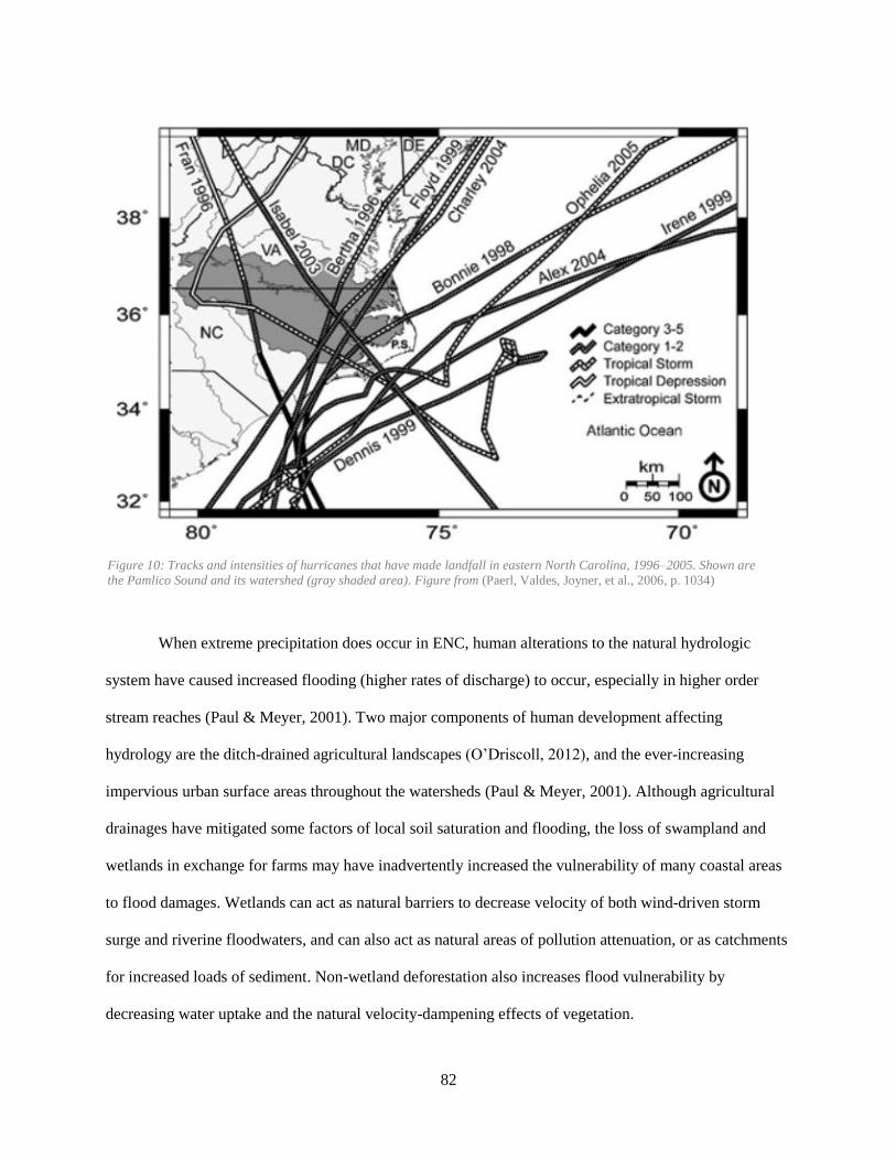
82
When extreme precipitation does occur in ENC, human alterations to the natural hydrologic
system have caused increased flooding (higher rates of discharge) to occur, especially in higher order
stream reaches (Paul & Meyer, 2001). Two major components of human development affecting
hydrology are the ditch-drained agricultural landscapes (O’Driscoll, 2012), and the ever-increasing
impervious urban surface areas throughout the watersheds (Paul & Meyer, 2001). Although agricultural
drainages have mitigated some factors of local soil saturation and flooding, the loss of swampland and
wetlands in exchange for farms may have inadvertently increased the vulnerability of many coastal areas
to flood damages. Wetlands can act as natural barriers to decrease velocity of both wind-driven storm
surge and riverine floodwaters, and can also act as natural areas of pollution attenuation, or as catchments
for increased loads of sediment. Non-wetland deforestation also increases flood vulnerability by
decreasing water uptake and the natural velocity-dampening effects of vegetation.
Figure 10: Tracks and intensities of hurricanes that have made landfall in eastern North Carolina, 1996–2005. Shown are
the Pamlico Sound and its watershed (gray shaded area). Figure from (Paerl, Valdes, Joyner, et al., 2006, p. 1034)
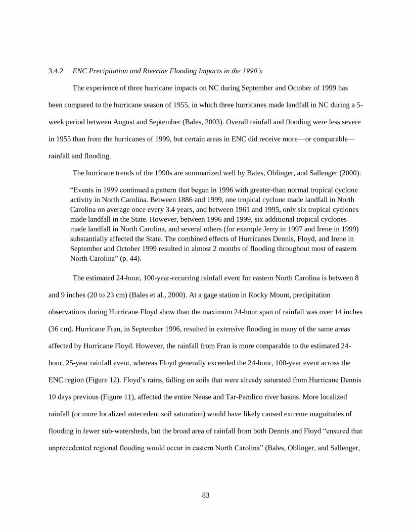
83
ENC Precipitation and Riverine Flooding Impacts in the 1990’s 3.4.2
The experience of three hurricane impacts on NC during September and October of 1999 has
been compared to the hurricane season of 1955, in which three hurricanes made landfall in NC during a 5-
week period between August and September (Bales, 2003). Overall rainfall and flooding were less severe
in 1955 than from the hurricanes of 1999, but certain areas in ENC did receive more—or comparable—
rainfall and flooding.
The hurricane trends of the 1990s are summarized well by Bales, Oblinger, and Sallenger (2000):
“Events in 1999 continued a pattern that began in 1996 with greater-than normal tropical cyclone
activity in North Carolina. Between 1886 and 1999, one tropical cyclone made landfall in North
Carolina on average once every 3.4 years, and between 1961 and 1995, only six tropical cyclones
made landfall in the State. However, between 1996 and 1999, six additional tropical cyclones
made landfall in North Carolina, and several others (for example Jerry in 1997 and Irene in 1999)
substantially affected the State. The combined effects of Hurricanes Dennis, Floyd, and Irene in
September and October 1999 resulted in almost 2 months of flooding throughout most of eastern
North Carolina” (p. 44).
The estimated 24-hour, 100-year-recurring rainfall event for eastern North Carolina is between 8
and 9 inches (20 to 23 cm) (Bales et al., 2000). At a gage station in Rocky Mount, precipitation
observations during Hurricane Floyd show than the maximum 24-hour span of rainfall was over 14 inches
(36 cm). Hurricane Fran, in September 1996, resulted in extensive flooding in many of the same areas
affected by Hurricane Floyd. However, the rainfall from Fran is more comparable to the estimated 24-
hour, 25-year rainfall event, whereas Floyd generally exceeded the 24-hour, 100-year event across the
ENC region (Figure 12). Floyd’s rains, falling on soils that were already saturated from Hurricane Dennis
10 days previous (Figure 11), affected the entire Neuse and Tar-Pamlico river basins. More localized
rainfall (or more localized antecedent soil saturation) would have likely caused extreme magnitudes of
flooding in fewer sub-watersheds, but the broad area of rainfall from both Dennis and Floyd “ensured that
unprecedented regional flooding would occur in eastern North Carolina” (Bales, Oblinger, and Sallenger,

84
p. 2). Additional rain from Hurricane Irene around October 14th, 1999 kept many areas above flood stage
towards the end of that month as well.
Figure 11: Rainfall in North Carolina, September 4-5, 1999, during the passage of Hurricane Dennis and locations of selected
rain gages in eastern North Carolina. (Rainfall map originally from the State Climate Office In North Carolina website, 1999)
Figure 12: Rainfall in North Carolina, September 14-16, 1999, prior to and during the passage of Hurricane Floyd. (Rainfall
map originally from the State Climate Office In North Carolina website, 1999)
It is important to note the variability in observed flood stages in different watersheds, and how
those compare to the estimated flood recurrence intervals at that time (Figure 13). In the Neuse river
basin, Bales, Oblinger, and Sallenger (2000) list 14 gage stations with stage height and discharge records
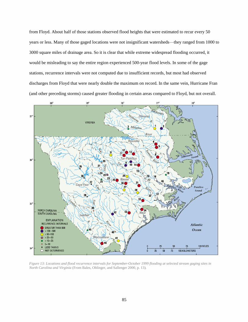
85
from Floyd. About half of those stations observed flood heights that were estimated to recur every 50
years or less. Many of those gaged locations were not insignificant watersheds—they ranged from 1000 to
3000 square miles of drainage area. So it is clear that while extreme widespread flooding occurred, it
would be misleading to say the entire region experienced 500-year flood levels. In some of the gage
stations, recurrence intervals were not computed due to insufficient records, but most had observed
discharges from Floyd that were nearly double the maximum on record. In the same vein, Hurricane Fran
(and other preceding storms) caused greater flooding in certain areas compared to Floyd, but not overall.
Figure 13: Locations and flood recurrence intervals for September-October 1999 flooding at selected stream gaging sites in
North Carolina and Virginia (From Bales, Oblinger, and Sallenger 2000, p. 13).
86
In addition to flood stages exceeding previous records across the ENC region, the length of time
that many areas in the Neuse and Tar-Pamlico remained above flood stage is another important factor to
note. From September through October, until many days after Hurricane Irene dumped additional (but
less extreme) rainfall, some areas never dipped below flood stage. The sheer volume of freshwater
flowing from the Tar-Pamlico River basin into the Pamlico Sound during the month of September 1999
was estimated to be at least 90% of the annual mean flow volume from that river basin (Bales et al.,
2000). Total freshwater inflow during September and October combined was also estimated to be over
80% of the total volume of the Pamlico Sound itself. Under average conditions, the expected flow would
be around 13% of the Sound volume during this period. Under normal conditions, water flowing through
the Tar-Pamlico and Neuse Rivers had a residence time of about 70 days, but mean water residence time
during September 1999 was estimated to be about 7 days. A lot of water was moving through these river
systems very rapidly.
The effects on water quality from Floyd in 1999 differed from Fran in 1996, according to water
quality measurements taken by USGS scientists (Bales & Childress, 1996; Bales et al., 2000).
Measurements of sustained hypoxic conditions (very low dissolved oxygen) that occurred in floodwaters
from Hurricane Fran did not occur after Hurricane Floyd. This may be due to higher and more sustained
flows that served to dilute materials that promote oxygen-consumption, relatively lower temperatures
after Floyd, or a slower floodwater recession that delivered organic materials more gradually from the
floodplains to the main river channels (Bales, Oblinger, and Sallenger 2000, p. 25). Outcomes of Fran’s
hypoxic conditions included extensive finfish and shellfish kills that lasted several weeks (Paerl,
Pinckney, Fear, & Peierls, 1998). These USGS scientists also note that despite this incredible dilution
(freshwater discharges of up to two orders of magnitude greater than the long-term September mean flow
in some places), concentrations of most pollutants were comparable to—or exceeded—the median levels
measured over the decade of 1990 to September 1999. This means that the total loads (total masses) of
nutrients and pollutants in the water were extremely high. For example, the total amount nitrogen
expected to pass Kinston on the Neuse River is about 3,400 tons, on average, over the course of a year.

87
About 50% of this amount was carried in Floyd floodwaters over a 36-day period (ibid, p. 45). At Tarboro
on the Tar River, Floyd’s floodwaters were estimated to carry close to 80% of the expected annual
nitrogen. The long-term fate and effects of these materials that were carried into, deposited, or attenuated
downstream in the Pamlico Sound is not clear, but research shows that the APES generally rebounded to
ecosystem equilibrium within one year (Paerl et al., 2001; Tester et al., 2003). There have been no long-
term impacts on water quality, although certain commercial estuarine species were impacted, especially
the blue crab (Burkholder et al., 2004; Paerl et al., 2006).
Sampling of Tar-Pamlico and Neuse River Basins for the bacteria Enterococcus coli and
Clostridium perfringens indicated that some sites had comparable or greater pathogen concentrations in
receding floodwaters, compared to measurements during peak flows (Bales, Oblinger, and Sallenger
2000, p. 30). C. perfringens is an indicator of environmentally resistant pathogens, but does not have a
USEPA criterion for acceptable concentrations in recreational waters (measured as colonies per 100
milliliters, or cols/100mL). The criterion for E. coli is 235 cols/100mL, and nearly every sample in the
Tar-Pamlico and Neuse River basins in September 1999 exceeded these levels, up to a maximum
observation of 13,000 cols/100mL in the Neuse River at Fort Barnwell (ibid).
1995 Oceanview Farm Waste Spill 3.4.3
Oceanview Farm was a 10,000-head swine confined animal feeding operation (CAFO) located in
the northwest corner of Onslow County in North Carolina (Figure 14). The lagoon at Oceanview Farm
was apparently one of the first in the state to be certified under new federal design specifications in 1993
(Warrick, 1995). In June of 1995, the lagoon was only 18 months old and had been inspected and certified
by the Natural Resource Conservation Service (Jackson et al., 1996). The farm managers had not
adequately been pumping out excess wastewater in the weeks leading up to a large rain event around June
18th, 1995. Up to 9 inches (23 cm) of rain may have fallen over the two weeks leading up to June 18
th.
Over the next few days, an additional 3 inches (8 cm) of rain soaked the landscape. On June 21st, the 12-

88
foot deep, 7-acre lagoon burst through a 30-foot wide section of the lagoon’s northeast wall, possibly
weakened by a newly installed irrigation pipe in addition to the heavy rains (ibid).
Oceanview Farm owners were unable to stop or repair the damage before the lagoon had emptied
its contents of more than 20 million gallons of swine waste. This nutrient-dense material spread across
neighboring forests and fields and ultimately into the stream network of the New River that passes
Jacksonville 20 miles downstream. This rapidly caused fish kills as the waste plume spread for miles
down the stream channel. The stream began recovering after about a week, but the event began making
headlines immediately, as it was unprecedented in scale and now party to a highly contentious debate
regarding swine CAFO regulation. The event was widely reported throughout the state and in national
media (Smothers, 1995). Although covered well by journalists, specific understanding of the cause of the
lagoon failure and the extent of its contamination were either not studied or not published in academic
literature, as inspection and monitoring was mainly conducted by state government and environmental
groups. Additional lagoon failures at other swine CAFO sites would occur that summer, which helped
spur legislative action for increasing swine CAFO regulation, which had otherwise been languishing in
state congress (Warrick & Leavenworth, 1995).

89
Figure 14: Aerial view of Oceanview Farm (now operated under a different name) in Onslow County, North Carolina. The waste
lagoon is approximately 7 acres, supporting over 10,000 head of finisher pigs. The bottom-right (northeast) corner of the lagoon
is where the breach was said to have occurred. 2012 Aerial imagery from NC One Map (www.nconemap.com).
Should the region expect increased flooding due to climate change and sea level rise? 3.4.4
The future effects of climate change on hurricane intensity and frequency impacting Atlantic
coastal regions like much of North Carolina are not yet well understood. However, many climatologists
have forecasted a general increase in storm frequency and intensity of Atlantic hurricanes over the rest of
this century (Knutson et al., 2010; Webster, Holland, Curry, & Chang, 2005).
The role of government in preparing for potential accelerated sea level rise (SLR) and climate
change through this century is currently a controversial issue in North Carolina. An NC state law passed
in 2012 (House Bill 819) banned state agencies from basing coastal policies on recent scientific
predictions about SLR, perhaps due to fears that alarmist anti-development in coastal areas would
significantly dampen a large sector of the NC economy in the short term (Phillips, 2012). The bill calls for

90
a study to be conducted, ending in 2015 (updating a previous SLR assessment from 2010), that presents
best-available peer-reviewed scientific hypothesis on sea level changes. The law does not affect county,
municipality, or other local government from making their own policies, but the Division of Coastal
Management and the Coastal Resources Commission are the only entities legally allowed to make state-
level decisions regarding SLR policy for all other state agencies to follow (NCGA, 2012).
According to the climate science articles cited in this section, and many other studies, a warming
atmosphere and sea surface ocean temperatures will probably strengthen the power of tropical cyclones
and hurricanes that develop in the Atlantic Ocean. With potentially stronger cyclones, combined with
expected SLR acceleration from increased ice melt and thermal expansion of ocean water, the ENC
region seems poised for increased challenges in its coastal region. Extreme precipitation, flooding,
ecosystem disturbance, and salt water intrusion over the coming century are just a few of the likely
challenges to be exacerbated by climate change; the degree of its effects are still poorly understood. As
the science continues to improve regarding climate change, the degree to which flood vulnerability may
increase in this region and elsewhere should become more solid. SLR impacts may begin affecting other
areas fairly soon, perhaps shifting the tide towards more resilience and adaptation policies for potential
challenges ahead.

4 GIS METHODS: FLOOD VULNERABILITY ASSESSMENT
4.1 Introduction
There has been widespread public concern in the ENC region regarding the potential human
health and environmental impacts of animal waste contamination during and after extreme rainfall events.
As mentioned in earlier sections, only one academic study (Wing et al., 2002) has analyzed the flood
vulnerability of industrial hog farms in ENC. This study made use of the swine CAFO permit coordinates
provided by the NC DWQ, but this data has spatial limitations and data quality issues that do not lend
well to a detailed analysis of flood vulnerability due to the large—and sometimes noncontiguous—area
covered by these agricultural sites. Extensive GIS analyses were performed in this study to delineate all
swine waste lagoon and housing structures at sites that are both active and inactive (expired or unknown
permits). These efforts have contributed significant corrections to the geospatial swine CAFO data and
have also improved their accuracy for flood vulnerability analysis.
4.2 Study Area
Delineation of every permitted swine operation in the state was not feasible due to the time and
effort required to accurately delineate and classify swine CAFO infrastructure. Instead, a limited study
area needed to be chosen for delineation, and it was preferred to have this area correspond with watershed
boundaries due to the hydrologic nature of flood analysis. Fortunately, these two criteria allowed for the
study site to cover the three main river basins for the Albemarle-Pamlico Estuary System (APES), which
has been the focus of much research regarding pollution and riverine floodwater impacts from hurricanes,
especially in the 1990’s (section 3.4.2). A map of the study area in Figure 15 shows the location of the
farm points and river basins included in the study area.
The study area contains approximately 1/3 of all active swine farm sites in NC. Only a few of the
these permitted sites could not be located due to outdated or inaccurate permit data, leaving 624 total

92
active sites that were included in the study area. Details of delineation of active swine farms, and the
discovery and delineation of 195 additional inactive swine farms sites are explained in section 4.4.
Figure 15: A map showing the study area of this project, which corresponds to the four major river drainage basins that make up
the Albemarle-Pamlico Estuary System. Individual swine farm sites are shown as points. Both the river basins and farm points
outside of the study area have been indicated by a shaded overlay.
4.3 Data
All data used for GIS analysis in this study were publicly available from NC government
websites and state-funded geospatial data repositories and streaming services. The primary source for
public geospatial data for the state is NC OneMap (www.nconemap.com). The NC Flood Mapping
Program (www.ncfloodmaps.com) also serves a wealth of geospatial information from its NC Flood Risk
Information System (FRIS) website (www.fris.nc.gov/fris), which contains all the FEMA-approved flood
hazard data used in this study. From OneMap, boundary shapefiles for NC counties, hydrologic units
(watersheds), and swine waste lagoon points were downloaded. Streaming aerial imagery services from

93
OneMap spanned the years 1993 to 2013, and were integral to the project. Other ancillary data from
OneMap that were helpful, but not integral to analysis were municipal boundaries, road networks, sewer
treatment plants, and streaming elevation data. The following subsections detail how this data was
prepared for the flood vulnerability analysis, and some of the data limitations for flood vulnerability
analysis.
Active Permitted Swine CAFO Locations and Waste Lagoons 4.3.1
Although OneMap hosts a shapefile for permitted CAFOs in NC, the attributes of those permit
points are missing information that is available in the active CAFO permit spreadsheet available from the
NC DWR website (NCDWR, 2015). Since the spreadsheet contains the same latitude and longitude
coordinates of each permitted operation, the spatial dataset was constructed from the spreadsheet rather
than from the OneMap source.
There is also a point shapefile hosted on OneMap that specifically delineates swine waste
lagoons, and this spatial information is not available elsewhere. Since this waste lagoon point dataset was
constructed as far back as 1998 using aerial imagery, alongside the creation of permit points by the DWQ,
this was critical in helping determine the locations of a large number of inactive swine CAFO sites,
including some that have been completely wiped off the map. It would have been nearly impossible to
have located many of these sites using aerial imagery. Even though the lagoon point features have no
attributes to indicate an associated permit number or other descriptive information, they were extremely
helpful. Points were generally well placed in the centroid of lagoons. Out of 4148 total lagoon points,
1413 (34%) were located in the study area.
The coordinates for the permitted swine CAFOs, however, had a significant amount of error in
their placement. The reason for the inaccuracies in placement were not clear, given the relatively more
accurate placement of lagoon points. For example, points were sometimes in the middle of a forested area
(Figure 16), hundreds of feet from a roadside location where a GPS unit most likely would have captured
a location point in 1998.

94
This led to much greater time spent using
ancillary data like Google Maps and Google Earth to
deduce the most likely match of permit point to visible
sites in aerial imagery. The inclusion of street addresses
in the spreadsheet, however, was helpful to track down
or confirm several questionable site locations with
missing, incomplete, or outdated address information.
The 20 fields of information available for each permit are
shown in Table 2Error! Reference source not found..
Table 2: The 20 fields of information provided in the NC DWR animal feeding operation permit spreadsheet (NCDWR, 2015).
NC 2015 Animal Permit Spreadsheet Information
Permit Number
Facility Name
Combined Owner
Regulated Operation
Permit Type
Regulated Activity
Allowable Count
Number Of
Lagoons
Issued Date
Effective Date
Expiration Date
Admin. Region
County Name
Location Latitude
Location Longitude
Address1 Address2 City State Zip
Sometimes multiple operation types (described in section 2.2.4) are located on the same physical
site, and share the same permit ID and identical attributes (including coordinates) aside from the operation
type and allowable head count. For the purposes of this study and for geospatial analysis, it was important
to collapse these multiple entries into a single “site” feature. The attributes for multiple operation types
were saved by adding extra fields (e.g. regulated operation 1; allowable animal count 1; regulation
operation 2; allowable count 2). Within the study site, there are 633 active swine CAFO sites. Of those
633 sites, 49 (8%) have more than one permitted operation type.
Figure 16: Example of an erroneous (off-site)
CAFO permit point (green) compared with the
lagoon point (red).

95
NC Flood Data and Geodatabase Files 4.3.2
The NC FRIS website provides geospatial flood data at the county level, and can be downloaded
in the ArcGIS file geodatabase (GDB) format. A GDB is essentially a proprietary data wrapper owned by
the company ESRI, whose GIS software and services are used by most government agencies. A GDB
contains geospatial files and information that can be stored more efficiently than individual shapefiles or
other discrete geospatial file formats. Within each NC county flood GDB there are a number of point,
line, and polygon feature classes (i.e. individual geospatial datasets). Only one feature class is critical to
this study, which is the flood hazard polygons that contain the official flood hazard areas created from
detailed and limited detailed flood studies. Depending on the county, this polygon feature class is named
“V_E_FLD_HAZ_AR” or “S_FLD_HAZ_AR.”
The flood GDBs are somewhat complex, and not user-friendly, as they are not intended for
dissemination of flood information to lay users, but rather for researchers, relevant industry users, or flood
mapping partners that are familiar their structure and content. The NC Floodplain Management branch
(NCFM) of the NC Division of Emergency Management prepared a very helpful “Quick Guide” in 2008
to introduce lay people to the components of various online flood map products, flood risk information,
and floodplain management and development issues (NCFM, 2008). The actual flood GDB design
information is contained in an 800-page technical document prepared by the NCFMP (last updated in
2014), which is also available online (NCFMP, 2014).
Flood GDB feature classes have no associated symbology, so it is important to understand which
fields and attributes correspond with flood hazard types in order to prepare the data properly for flood
vulnerability analysis. For this study, flood vulnerability was prepared by defining relevant flood hazard
polygons to be those in the A and AE zones (1% annual chance of flooding). These combined flood zones
are shown within the study area in Figure 17. Coastal VE flood zones (1% annual chance of experiencing
storm surge wave heights of 1 meter or more) were examined but not included, as their boundaries were
over 2.4 kilometers (1.5 miles) from any known (active or inactive) swine CAFOs.

96
Figure 17: Combined A, AE, and 500-year flood zones shown in blue within the study area (unshaded portion).
Aerial Imagery 4.3.3
Streaming aerial imagery services spanning the years 1993 to 2013 were used in the course of this
study. It is relevant to note that there were many sources of the aerial image tiles that are hosted on
OneMap, and although a year is often used to describe each collection, they are essentially a mosaic of
imagery tiles that may have been captured over a span of many months. However, general purpose
imagery is usually captured during the period of the year without deciduous tree cover (late fall or winter)
in order to increase visibility. A few of these imagery sets are described because of their importance for
the study. In only a few cases, imagery from Google Maps was used for delineation. Attributes of Google
imagery is not provided, but it was at least more recent than OneMap imagery because it revealed newly
reconstructed swine housing in a few cases.
One Map’s most recent high-resolution imagery for the ENC region combines coverage from
aerial imagery flown in 2012 and 2013, with a pixel resolution of 6 inches (15 cm). State-wide imagery is
available for the year 2010, but the data captured during 2012 to 2014 were for discrete areas (Figure 18).
Imagery from 2010 to date is part of a state imagery acquisition plan that began in 2009 (NCGICC, 2008,
2010). Only 2 active and 2 inactive operations are located within the 2014 imagery area, so that was not
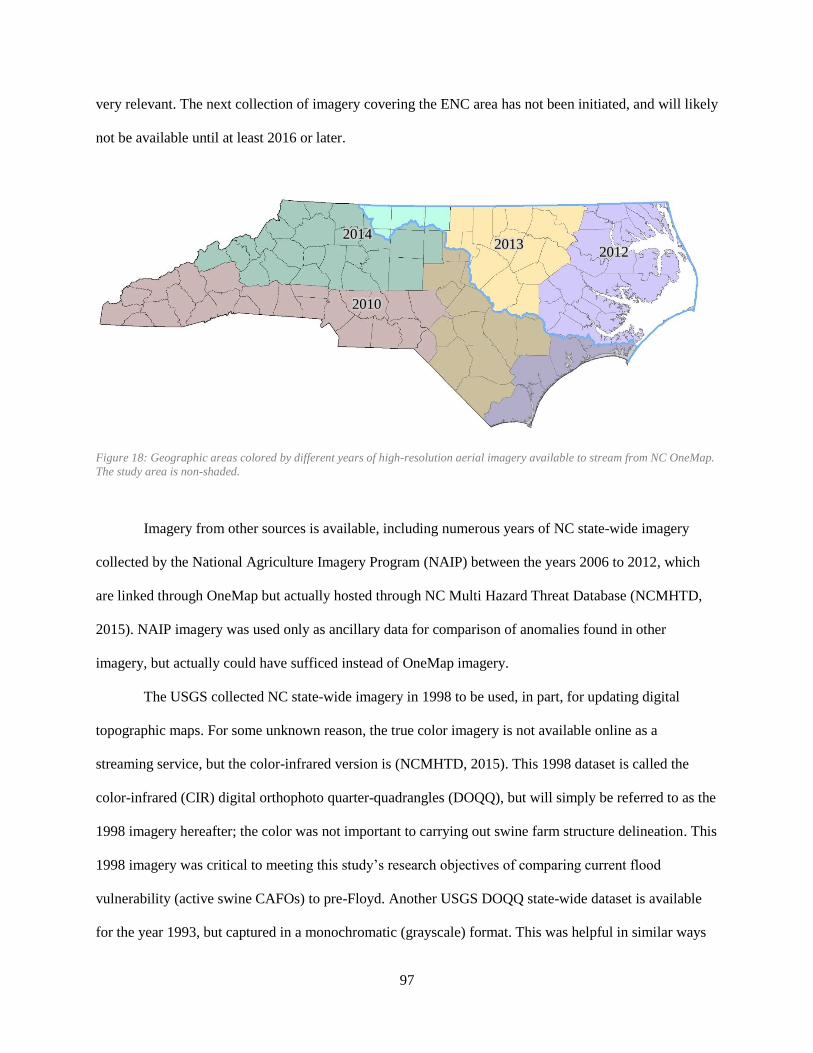
97
very relevant. The next collection of imagery covering the ENC area has not been initiated, and will likely
not be available until at least 2016 or later.
Figure 18: Geographic areas colored by different years of high-resolution aerial imagery available to stream from NC OneMap.
The study area is non-shaded.
Imagery from other sources is available, including numerous years of NC state-wide imagery
collected by the National Agriculture Imagery Program (NAIP) between the years 2006 to 2012, which
are linked through OneMap but actually hosted through NC Multi Hazard Threat Database (NCMHTD,
2015). NAIP imagery was used only as ancillary data for comparison of anomalies found in other
imagery, but actually could have sufficed instead of OneMap imagery.
The USGS collected NC state-wide imagery in 1998 to be used, in part, for updating digital
topographic maps. For some unknown reason, the true color imagery is not available online as a
streaming service, but the color-infrared version is (NCMHTD, 2015). This 1998 dataset is called the
color-infrared (CIR) digital orthophoto quarter-quadrangles (DOQQ), but will simply be referred to as the
1998 imagery hereafter; the color was not important to carrying out swine farm structure delineation. This
1998 imagery was critical to meeting this study’s research objectives of comparing current flood
vulnerability (active swine CAFOs) to pre-Floyd. Another USGS DOQQ state-wide dataset is available
for the year 1993, but captured in a monochromatic (grayscale) format. This was helpful in similar ways
2014
2012 2013
2010

98
to the 1998 imagery in determining locations of inactive CAFOs, but not as relevant to confirming pre-
Floyd sites, since some had not yet been fully constructed or expanded in 1993. The specific 1998 pixel
resolution is not clear, but it is actually lower than the 1993 imagery, which is approximately 1 foot (0.3
meters). Although the 1998 imagery lacked as much spatial detail, the large size of swine housing and
waste lagoons made this a non-issue.
Figure 19: A comparison of three aerial imagery datasets used in this study, as described above. The image extent is focusing on
a large swine farm within Greene County that was active at least as recently as 1998, but its buildings were likely destroyed by
flood damage by Hurricane Floyd and it was abandoned as a swine production facility (this site is within the current FEMA 100-
year floodplain). No record of its permit exist in an electronic form. This site is treated as an “unknown” inactive swine farm site
that definitely was active before Floyd.
Digital Elevation Model (3-meter Resolution) 4.3.4
The current National Elevation Dataset (NED) includes a 3-meter resolution digital elevation
model (DEM)5 for the entire state of North Carolina. This level of resolution is not available in a raster
DEM format from the NCFMP’s website. NCFMP provides 20-foot (6-meter) DEMs for each NC county,
but this resolution was insufficient to pick up the lagoon berm elevation heights; 20-foot resolution
generally aggregates (averages) too wide of an area such that the maximum berm elevation “lip” values
are lost to the much lower surrounding elevation. NED (3-meter) tiles were downloaded and mosaicked to
achieve a completely dataset for the study area. This data is freely available from the USGS “National
Map” download service online (USGS, n.d.).
5 The resolution of these tiles is actually 1/9 arc-second, which is approximately 3 meters or 10 feet.

99
4.4 Methods
Delineating and Classifying Active CAFO Infrastructure 4.4.1
Delineation of permitted swine CAFO housing and lagoons (referred to in this section
collectively as “units”) began as a straightforward process of tracing units, and assigning those polygons a
class and a permit ID. Housing units were traced based on roof corners, and lagoons were traced up to the
perceived inner edge of the berm, rather than the visible water level6. The workflow soon became bogged
down in a more involved exercise of analysis and judgment for accurate classification or exclusion of
certain buildings in the data set. Attention to detail was necessary to determine with greater confidence
which units should be considered “active,” and, more importantly, which units actually belong to each
permit ID. As the classification process and workflow evolved, units were given the value “H” for active
housing, “D” for destroyed or damaged (assumed inactive) housing, and “L” for active lagoons7. Each of
these units was attributed to a permit ID.
As mentioned in the data section (4.3.1), the permit coordinates provided by the DWR are often
erroneous. A bit of detective work was required to maximize confidence when associating units with
ambiguously-placed permit points. The street address and “number of lagoons” fields were most often
helpful in this regard. Points representing each site were later updated to equal the centroid (spatial
center) of all unit polygons associated with that ID. This enables quantification of error in the original
permit point dataset, and to compare the difference in flood vulnerability results when using the updated
point locations.
Some expired operations continue to exist in the spreadsheet even though they did not renew their
permits for the year 2015 and beyond. These are sites with outstanding issues and have not yet been
formally shut down or re-permitted, and thus maintain their active permit status and continue to have
6 Because of discrepancies in georectification of aerial imagery, and some level of user error in delineation, it is estimated that
housing units were delineated +/- 5 meters from actual corner points. Lagoons may be similarly inaccurate due to the ambiguous
definition of the upper lagoon berm “ridge” or “lip,” and being able to perceive where any such edge is in the available aerial
imagery; it is estimated that lagoon polygon boundaries were delineated with +/- 8 meters from actual berm lip centers. 7 Inactive or obviously non-waste lagoons or ponds next to permitted operations were sometimes classified as “P” for ponds. This
helped when revisiting sites and for quality control measures later on, since such ponds can easily be mistaken for lagoons at a
glance. However, these ponds are not factored into flood-related analysis.

100
inspections like other operations (Deborah Watts, Program Manager of NC DWR Animal Feeding
Operations, personal communication, June 12, 2015). Other permits in the spreadsheet may have not yet
actually exceeded the listed expiration date, but are listed with zero allowable head count for similar
reasons (ibid). In both of these cases, the sites were delineated normally, but the associated permit points
were assigned a different “expired” class to indicate they are not active.
Classification of units was performed with much care and consideration, as a number of realities
may not be apparent at first glance in aerial imagery. Many types of agricultural buildings looks similar to
swine housing, especially poultry CAFO housing. Over time, one gets a feel for what is most likely
poultry housing because these generally have more extreme length to width ratios. However, swine
housing shapes can be highly variable, and sometimes the scale of buildings makes it difficult to initially
determine size without measuring and comparing footprint area to other sites; length to width was not
always the best initial determinant. Possible poultry units are sometimes situated right next to swine units,
in which case the allowable head count and operation type were reviewed to make a determination if
certain buildings include a feasible area to house that many swine, or if the other buildings are, in fact,
more likely to be part of the operation (two examples are shown in Figure 20).
Figure 20: Two examples of poultry CAFO buildings in very close proximity to swine CAFO buildings. Only the swine CAFO
housing and lagoons are delineated and classified. Aerial imagery from 2013, provided by the NC One Map service.
0 30 6015Meters
0 100 20050Feet
0 40 8020Meters
0 130 26065Feet
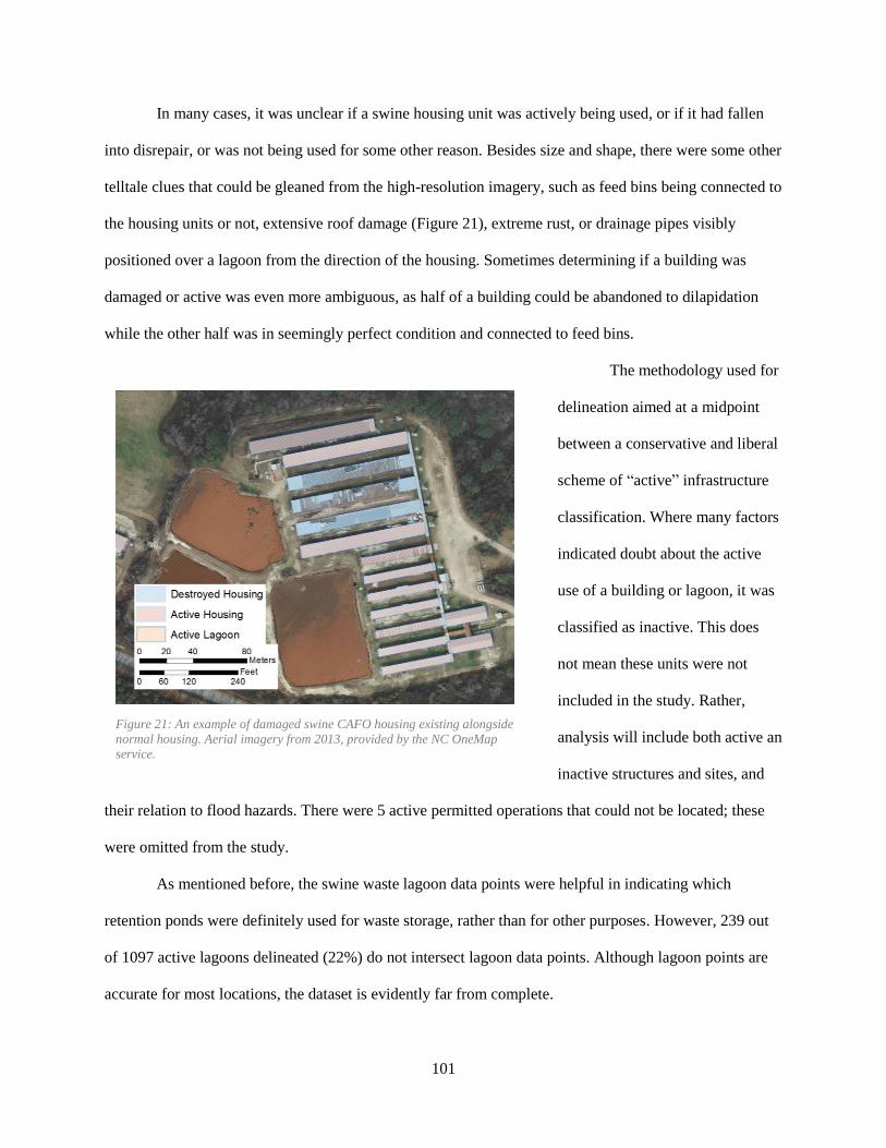
101
In many cases, it was unclear if a swine housing unit was actively being used, or if it had fallen
into disrepair, or was not being used for some other reason. Besides size and shape, there were some other
telltale clues that could be gleaned from the high-resolution imagery, such as feed bins being connected to
the housing units or not, extensive roof damage (Figure 21), extreme rust, or drainage pipes visibly
positioned over a lagoon from the direction of the housing. Sometimes determining if a building was
damaged or active was even more ambiguous, as half of a building could be abandoned to dilapidation
while the other half was in seemingly perfect condition and connected to feed bins.
The methodology used for
delineation aimed at a midpoint
between a conservative and liberal
scheme of “active” infrastructure
classification. Where many factors
indicated doubt about the active
use of a building or lagoon, it was
classified as inactive. This does
not mean these units were not
included in the study. Rather,
analysis will include both active an
inactive structures and sites, and
their relation to flood hazards. There were 5 active permitted operations that could not be located; these
were omitted from the study.
As mentioned before, the swine waste lagoon data points were helpful in indicating which
retention ponds were definitely used for waste storage, rather than for other purposes. However, 239 out
of 1097 active lagoons delineated (22%) do not intersect lagoon data points. Although lagoon points are
accurate for most locations, the dataset is evidently far from complete.
Figure 21: An example of damaged swine CAFO housing existing alongside
normal housing. Aerial imagery from 2013, provided by the NC OneMap
service.

102
Delineation of Former (unknown) Swine CAFOs 4.4.2
After delineation of active sites was complete, it was assumed that any other swine CAFO sites
with waste lagoons found (using 1998 imagery) in the study area would be operations that were active in
1998. No new operations were built after that point. Lagoon points were extremely helpful in indicating
where former sites were located. Without the help of the lagoon points, only a fraction of the inactive
swine CAFO sites would have been found. Each lagoon point was reviewed with 1998 imagery and
delineated based on that information. Sites or infrastructure that could not be confidently considered part
of swine operations from either the 1998 or 1993 imagery were omitted. In addition, an archived permit
spreadsheet from 2004 was acquired from the DWR office to help confirm as many old sites as possible.
Permit data from before 2004 is not available (Deborah Watts, Program Manager of NC DWR Animal
Feeding Operations, personal communication, June 12, 2015).
Figure 22: An example of a swine farm site that was active in 1998, but virtually "wiped off the map" by 2013. It would be
virtually impossible to have concluded from 2013 areal imagery that this was a former swine farming site. The two lagoon points
(from the swine waste lagoon point shapefile) for this location were the only indication that this area should be investigated for a
potential inactive swine farm. There are many more examples like this in the study area.
Some of the sites that were active in 1998 are completely wiped off the map in most recent aerial
imagery (Figure 22). Infrastructure on unknown sites that still looked like well-maintained swine housing
were classified as “H?”, to be distinguished from the active “H” units. Likewise, “D?” for damaged or
destroyed buildings, and “L?” for waste lagoons. Even if a lagoon was completely filled in and reclaimed

103
as an agricultural field in the recent imagery, it was still delineated as the lagoon existed in 1998, for
purposes of “pre-Floyd” flood vulnerability analysis. Each unknown site had a point created for it, and
was assigned a unique ID. The delineated unknown infrastructure was assigned the corresponding ID like
active sites. Unknown points did not have any extra information about the operation like active sites, but
they were necessary for counting the number of “sites” versus only having a collection of unknown
infrastructure units.
Delineation of Lagoon Buyout Program Participants 4.4.3
Unpublished documents explaining various aspects of the lagoon buyout program were obtained
from the NC Soil and Water Conservation (SWC), a division of the NC Department of Agriculture and
Consumer Services. One of these documents contains details about the hog operations that participated in
the waste lagoon buyout program over the years 1999 to 2008 (CWMTF, 2008), as discussed in section
2.3.9. SWC also has an interactive “easement viewer” mapping application online that displays all of the
location and outlines of easements granted and completed in the buyout program (NCDACS, n.d.).
There were 42 total operations that were bought out and prepared for closure under the
supervision of the SWC. The document and easement viewer were used to find and delineate the 31
buyout operations located within the study site, and assign attributes for each farm’s permitted head count
and operation type at the time of closure. One operation was missing from the easement viewer at the
time of this study but will be fixed later (David Williams, deputy director of SWC, personal
communication, June 16th, 2015). It is interesting to note that most of these buyouts are located within the
study area, which contains only about one third of all active swine operations. As the buyout program was
the most direct action undertaken by the state to mitigate the existing flood vulnerability of the industry,
these operations are analyzed and discussed in the next chapter.

104
Relating CAFOs to Floodplains 4.4.4
ArcGIS and similar geospatial software include tools to perform common geospatial tasks that
can extract, join, and relate different layers of data. These tools were used to calculate the distance of each
CAFO site (point) and each CAFO unit (polygon) to their nearest flood zone boundary. Information about
the nearest flood zone, including its type (AE, A, or 500-year) and other relevant attributes were joined to
each site point or unit polygon.
Floodplain boundary uncertainty and the importance of structure elevation in relation to the BFE
has been discussed in section 3.3. It is clear that analyzing the distance to nearest flood zone is an
interesting exploratory measure of flood vulnerability, but it is also very crude as a metric for analyzing
the real risk of inundation and structural damage of CAFO infrastructure, which would likely lead to
water contamination issues. The detail in the topographic area between a modeled flood hazard boundary
and CAFO infrastructure can be extremely important, even when the distance is fairly small. The
elevation of lagoon berms and first floor elevations of housing would also affect the relative risk of each
structure to flood damages. However, the inundation of only parts of a structure—even if not completely
flooded or overtopped in the case of lagoons—can still have impacts on structural integrity by directly
eroding or by saturating lagoon walls, which can potentially lead to liquefaction of a section of the
structure. In the case of swine housing, some amount of waste is contained within these buildings as well,
and the swine themselves become a potential water contamination hazards if they were to drown within or
outside of a building, and begin to decay.
To approach a more realistic modeling of flood vulnerability than distance to floodplain, high
resolution LiDAR elevation (Z) data was acquired to explore a methodology that further incorporates
topographic variability, and Z differences of lagoons and housing to nearest base flood extent. This
methodology could be applied state-wide with the 3-meter resolution DEM available from the USGS’s
NED. Even higher resolution data (0.5 meter resolution) will soon be available for the entire state.
Unfortunately, the time required to download and process this extremely dense elevation dataset for large
regions of the state is beyond the scope of this project.

105
One of the primary benefits of high-resolution elevation data is being able to (approximately)
capture each lagoon’s maximum berm height, which then allows more accurate analysis of the Z-
difference to nearest floodplains. However, topographic variability of floodplains can enable water to
more easily reach certain areas of the stream valley slopes through non-linear pathways.
The DEM raster can also be used to calculate a “cost-distance” for water to travel from a source
location (e.g. flood hazard area) in three dimensions (Douglas, 1994). Cost-distance calculations simulate
the accumulative “impedance” of moving across a grid with varying “cost” values, such as an elevation
surface (slope) in this case (Brivio, Colombo, Maggi, & Tomasoni, 2002). Other applications of cost-
distance can integrate many more cost variables besides slope. For example, to help determine the most
viable route (least cost path) for new roads or utility easements, rasters representing land-use or zoning
areas, existing developments, and soil characteristics can all be separately classified into numeric “cost”
rankings, weighted depending on importance, and then integrated to create a total “cost surface” (Bagli,
Geneletti, & Orsi, 2011; Yu, Lee, & Munro-Stasiuk, 2003). A single least-cost path or series of paths can
then be calculated.
Figure 23: An ArcGIS modelbuilder diagram of the cost-distance model for creating the cost-distance raster used in this study.
See next figure (Figure 24) below for an example of the cost-distance raster symbolized for visual analysis.

106
In this study, only elevation change (slope) is used as the cost variable, and the least cost paths
themselves are not as important as determining the least cost-distance values for floodwaters to reach
each swine farm structure, for relative comparison. Although water certainly does encounter resistance
when moving horizontally across almost all surfaces due to surface roughness and vegetation cover, this
would be complex to model across the entire study area and likely insignificant for the purpose of
ultimately creating a qualitative vulnerability index in this study. Therefore, horizontal cost is considered
to be a constant value of 1 for each consecutive cell distance traveled. The vertical factor, however, must
incorporate elevation changes from one cell to the next. A “slope” raster (cell values of slope in degrees)
was processed from the DEM and used as the cost variable for moving between each cell. Cost-distance
helps incorporate a more realistic representation of water’s natural tendency to follow a path of least
resistance when flood stages rise; this does not always occur in straight lines. A diagram of the ArcGIS
model builder process is shown in Figure 23.
Cost-distance was calculated from the 100-year floodplain boundaries within the study area, up to
a certain arbitrary limit—since these calculations were very processing-intensive, it was not helpful to
calculate cost-distances representative of an unfeasible, biblical flood stage. The calculated cost-distance
raster area actually reached 10 meters (35 feet) above the base flood (100-year) elevation in most places,
which, it is safe to say, surpasses feasible flood stages. However, this was helpful for visualizing the
variability of cost-distance from floodplains within different stream reaches. The output of the cost-
distance processing was a cost-distance mosaic spanning all parts of the study area where floodplain
information exists (localized example in Figure 24). Lagoon and housing polygons were then intersected
with this cost-distance raster using the zonal statistics as table tool to extract cost-distance values for the
vulnerability index, as described in the next section.
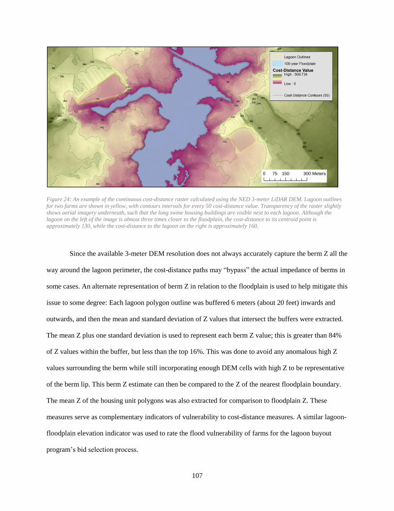
107
Figure 24: An example of the continuous cost-distance raster calculated using the NED 3-meter LiDAR DEM. Lagoon outlines
for two farms are shown in yellow, with contours intervals for every 50 cost-distance value. Transparency of the raster slightly
shows aerial imagery underneath, such that the long swine housing buildings are visible next to each lagoon. Although the
lagoon on the left of the image is almost three times closer to the floodplain, the cost-distance to its centroid point is
approximately 130, while the cost-distance to the lagoon on the right is approximately 160.
Since the available 3-meter DEM resolution does not always accurately capture the berm Z all the
way around the lagoon perimeter, the cost-distance paths may “bypass” the actual impedance of berms in
some cases. An alternate representation of berm Z in relation to the floodplain is used to help mitigate this
issue to some degree: Each lagoon polygon outline was buffered 6 meters (about 20 feet) inwards and
outwards, and then the mean and standard deviation of Z values that intersect the buffers were extracted.
The mean Z plus one standard deviation is used to represent each berm Z value; this is greater than 84%
of Z values within the buffer, but less than the top 16%. This was done to avoid any anomalous high Z
values surrounding the berm while still incorporating enough DEM cells with high Z to be representative
of the berm lip. This berm Z estimate can then be compared to the Z of the nearest floodplain boundary.
The mean Z of the housing unit polygons was also extracted for comparison to floodplain Z. These
measures serve as complementary indicators of vulnerability to cost-distance measures. A similar lagoon-
floodplain elevation indicator was used to rate the flood vulnerability of farms for the lagoon buyout
program’s bid selection process.
0 150 30075 Meters

108
Constructing an Index of Flood Vulnerability 4.4.5
The construction of the flood vulnerability index in this study involves normalizing three
quantitative measures in order to integrate them together as qualitative (ranked) indicators of
vulnerability. This is done by integrating the individual housing and lagoon structure vulnerability
measures first, and then further integrating these structure-level indicators into a measure for each farm
site as a whole. As discussed in section 3.2Error! Reference source not found., vulnerability is
arrowly defined in this study as the bio-physical exposure of swine housing and waste lagoons to
estimated 100-year recurring flood hazards, and for even greater flood hazards beyond that. Greater
flooding can certainly occur throughout the study area, as Hurricane Floyd dramatically proved.
Uncertainty in flood mapping studies, as discussed in section 3.3.1, also suggests that vulnerability should
be considered beyond the estimated 100-year flood areas, as current estimates are far from perfect. Flood
stages could potentially be under-estimated vertically by a number of stream reaches; each additional
vertical distance unit of flood stage can translate to tens of distance units horizontally in many parts of the
flat ENC landscape.
The following quantitative components are used to construct the index of vulnerability for
individual lagoon and housing structures:
1. Cost-distance (from the 100-year floodplains):
o For housing: the average cost-distance intersecting housing polygons.
o For lagoons: the minimum8 (least) cost-distance intersecting the lagoon polygon outlines
(not buffered).
2. Elevation difference from nearest 100-year floodplain to…
o For housing: the mean elevation of the swine housing polygons.
o For lagoons: the mean +1 standard deviation of lagoon berm elevation (using a 6-meter
buffer of lagoon outline).
3. Distance to the nearest9 100-year floodplain for both housing and lagoon polygons.
8 Using the minimum value is important here to incorporate the directionality of cost-distance pathway, which will generally
interact with the lagoon berm outline at the closer points first. Using the mean value would include cost-distance values out to the
furthest reaches of lagoon, rather far away from the closest points of flood contact. Housing is relatively flat, and much smaller,
so taking the mean cost-distance makes more sense as it will vary little. 9 Lagoon and housing units are only related to floodplains within their immediate watershed (HUC-12), which helps avoid cases
of nearby floodplains that are actually across a watershed divide. This would misrepresent the longer distance to the nearest
floodplain of consequence for certain locations.

109
The values from each of these three measures were classified into five ranks of relative
vulnerability (Error! Reference source not found.), with 4 being most vulnerable and 0 being least
ulnerable10
. This serves to “normalize” the different measures into comparable qualitative rankings.
Because cost-distance integrates both components of elevation difference and distance to nearest
floodplain, the cost-distance rank (Cdist) was multiplied by 2, while the elevation difference rank (Zdiff)
and the distance to floodplain rank (Fdist) were added together. These values were then added together,
becoming the integrated ‘structure flood vulnerability rank’ (Vstructure), with a maximum of 16 (most
vulnerable) and minimum of 0 (least vulnerable)(Equation 1). For each farm site, the arithmetic mean of
all of that farm’s structures’ Vstructure values is calculated, becoming the overall integrated ‘farm flood
vulnerability rank’ (Vfarm) (Equation 2). Vfarm ranks also have a maximum value of 16 (most vulnerable)
and minimum of 0 (least vulnerable).
Table 3: Class breaks for flood vulnerability rankings for the three vulnerability indicators
Rank
Cost-Distance Z-Difference Above
Floodplain Distance to Floodplain
(non-unit measure)
(feet) (meters)
(feet) (meters)
4 < 10
< 3 < 0.9
< 50 15
3 10 to 50
3 to 6 0.9 to 1.8
50 to 150 15 to 46
2 50 to 150
6 to 8 1.8 to 2.4
150 to 250 46 to 76
1 150 to 300
8 to 10 2.4 to 3
250 to 350 76 to 107
0 > 300
>10 > 3
> 350 > 107
Equation 1: Calculation of each swine farm structure’s flood vulnerability
Vstructure = (Cdist * 2) + (Zdiff + Fdist)
Equation 2: Calculation of each swine farm site’s flood vulnerability
10
Structures without elevation or cost-distance data are considered 0 rank (least vulnerable). Structures with negative Z-
difference to floodplain (below the nearest floodplain elevation) were inspected and confirmed to be in the floodplain.

110
________
Vfarm = Vstructure
The farm flood vulnerability rank was slightly complicated by the need to assess active swine farms
and their currently-active structures in 2013 without including structures that have been deemed to be
damaged or destroyed some time before 2013. For current (2013) farm vulnerability rankings, all
damaged or destroyed structures were omitted from the integrated farm vulnerability ranking. For pre-
Floyd (1998) farm rankings, all structures are included since all structures are assumed to have been
active in 1998 with very few exceptions (e.g. rebuilt housing due to disrepair in recent years). In this way,
a meta-ranking of industry-wide farm vulnerability can be calculated by comparing the sum of current
farm vulnerability rank values (2013) to those from pre-Floyd (1998).

5 RESULTS AND DISCUSSION
5.1 Overall Site Vulnerability Results
This chapter reviews and discusses the results of the GIS methodology. A number of figures and
maps are used to help illustrate the findings and inform discussion of the results from certain spatial
perspectives (e.g. hydrologic, by county). This chapter answers the primary research question of the
thesis: “how does current hog farm flood vulnerability in ENC compare with vulnerability before
Hurricane Flood?” Vulnerability is clearly shown to decrease overall, but the patterns of this change are
interesting, and some aspects are surprising. Figure 25 below shows the study area with swine farm points
symbolized based on active, inactive, or lagoon buyout participant classifications. Although inactive sites
seem to be distributed all over the study area, the majority of the most highly vulnerable sites were
located in lowland river basin areas closest to the Albemarle and Pamlico Sounds, between the Tar-
Pamlico River mouth and the Albemarle Sound.
Figure 25: A map showing the active, inactive, and buyout participant swine farm sites within the study area.
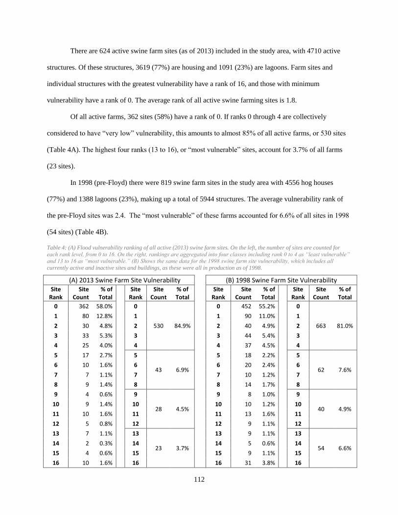
112
There are 624 active swine farm sites (as of 2013) included in the study area, with 4710 active
structures. Of these structures, 3619 (77%) are housing and 1091 (23%) are lagoons. Farm sites and
individual structures with the greatest vulnerability have a rank of 16, and those with minimum
vulnerability have a rank of 0. The average rank of all active swine farming sites is 1.8.
Of all active farms, 362 sites (58%) have a rank of 0. If ranks 0 through 4 are collectively
considered to have “very low” vulnerability, this amounts to almost 85% of all active farms, or 530 sites
(Table 4A). The highest four ranks (13 to 16), or “most vulnerable” sites, account for 3.7% of all farms
(23 sites).
In 1998 (pre-Floyd) there were 819 swine farm sites in the study area with 4556 hog houses
(77%) and 1388 lagoons (23%), making up a total of 5944 structures. The average vulnerability rank of
the pre-Floyd sites was 2.4. The “most vulnerable” of these farms accounted for 6.6% of all sites in 1998
(54 sites) (Table 4B).
Table 4: (A) Flood vulnerability ranking of all active (2013) swine farm sites. On the left, the number of sites are counted for
each rank level, from 0 to 16. On the right, rankings are aggregated into four classes including rank 0 to 4 as “least vulnerable”
and 13 to 16 as “most vulnerable.” (B) Shows the same data for the 1998 swine farm site vulnerability, which includes all
currently active and inactive sites and buildings, as these were all in production as of 1998.
(A) 2013 Swine Farm Site Vulnerability
(B) 1998 Swine Farm Site Vulnerability Site
Rank Site
Count % of
Total
Site Rank
Site Count
% of Total
Site Rank
Site Count
% of Total
Site
Rank Site
Count % of Total
0 362 58.0% 0
530 84.9%
0 452 55.2% 0
663 81.0%
1 80 12.8%
1
1 90 11.0%
1
2 30 4.8%
2
2 40 4.9%
2
3 33 5.3%
3
3 44 5.4%
3
4 25 4.0%
4
4 37 4.5%
4
5 17 2.7%
5
43 6.9%
5 18 2.2%
5
62 7.6% 6 10 1.6%
6
6 20 2.4%
6
7 7 1.1%
7
7 10 1.2%
7
8 9 1.4%
8
8 14 1.7%
8
9 4 0.6%
9
28 4.5%
9 8 1.0%
9
40 4.9% 10 9 1.4%
10
10 10 1.2%
10
11 10 1.6%
11
11 13 1.6%
11
12 5 0.8%
12
12 9 1.1%
12
13 7 1.1%
13
23 3.7%
13 9 1.1%
13
54 6.6% 14 2 0.3%
14
14 5 0.6%
14
15 4 0.6%
15
15 9 1.1%
15
16 10 1.6% 16
16 31 3.8% 16

113
A total of 195 sites have become inactive since 1998, and their vulnerability can be reviewed
independently as a group. Of these inactive sites, 10.8% have the maximum vulnerability rank of 16, and
15.9% are rank 13 or higher, or “most vulnerable” (Figure 26). It is interesting to note that, of the 30
lagoon buyout sites that are included in the 195 inactive sites, only 18 buyout sites are of “most
vulnerable” rank. This is discussed further in section 5.4. The much higher rate of vulnerable structures
among the inactive sites suggests that flood impacts from Floyd have played a significant role in the
removal of farms from production since 1998.
Figure 26: Active vs. inactive swine farm site vulnerability. This table helps show the relatively high concentration of
vulnerability among the farms that have become inactive since 1998.
These results do not sustain the original hypothesis that a majority of vulnerable farm sites remain
in production to this day. Only 23 out of 54 (43%) most vulnerable farm sites, and 170 out of 437
individual most vulnerable swine farm structures (39%) remain in operation as of 2013. However, this
rate of remaining vulnerable swine CAFOs is still at a concerning level and worthy of further
investigation beyond this study.
81.0%
7.6% 4.9% 6.6%
67.7%
9.7% 6.7%
15.9%
0.0%
10.0%
20.0%
30.0%
40.0%
50.0%
60.0%
70.0%
80.0%
90.0%
"Least" (0 to 4) "Low" (5 to 8) "Medium" (9 to 12) "Most" (13 to 16)
Pe
rce
nt
of
Swin
Far
m S
ite
s
Flood Vunlerability Rank
Active vs Inactive Site Vulnerability
Active Inactive

114
5.2 Spatial Distribution of Vulnerability
There appears to be an overall spatial distribution of vulnerability in 1998 that was skewed
towards the low central-eastern and north-eastern coastal areas; 2013 vulnerability distribution is
dramatically less skewed towards the coast as many of those most highly vulnerable farms have been
removed from production since 1998. Figure 27 illustrates these findings through standard deviational
ellipses (directional distribution), processed using site vulnerability as the spatial weight; sites from 2013
(active only) and 1998 (active and inactive) sites were processed separately. These ellipses show that
vulnerability was more heavily skewed towards the low coastal areas north of the Tar-Pamlico River in
1998, but a large number of these vulnerable sites have since been removed; farm vulnerability—and
swine farming overall—is less extensive in this area now. There seems to be a remaining vulnerable area
“hot-spot” centered in the Neuse River Basin (lower-left of Figure 27). This is further analyzed in the next
sub-section regarding vulnerability from a hydrologic (river sub-basin) perspective (Figure 28).

115
Figure 27: Directed (weighted) distribution of site flood vulnerability rankings, calculated for 2013 sites, 1998 sites, and inactive
sites separately. The remaining vulnerable “hot-spot” in the Neuse River area in the bottom-left area of this map is illustrated
well in Figure 28 below.
5.3 Vulnerability from a Hydrologic (River Sub-Basin) Perspective
Instead of site ranking, results for hydrology (river sub-basins) focus on counts of individual
vulnerable structures. Out of 5944 total structures, 437 were at least rank 13, which are considered the
“most vulnerable” structures. Collectively, these serve as a proxy measure for net vulnerability for each
sub-basin. Of these 437 most vulnerable structures, only 170 (39%) were still active in 2013.
The comparative loss of these vulnerable structures from each river sub-basin in the study area is
shown in Figure 28, and this data is also presented in Table 5. The Pamlico and Albemarle sub-basins
have lost the greatest total number of highly vulnerable structures since 1998—especially the Albemarle,
which today only has 9 out of 103 still in production. The Pamlico sub-basin has retained 27 out of 87
structures, and the Pamlico Sound sub-basin has lost all of its 30 vulnerable structures.

116
Figure 28: Number of the "most vulnerable" structures within each river sub-basin (HUC-8 watershed areas). Totals are
represented and compared between the 1998 and 2013 industry with representative bar/column symbols.Actual values of number
of “most vulnerable” sites are labeled for each sub-basin, with the 1998 on the left (red), and the 2013 on the right (yellow).
The Middle Neuse has also lost a substantial amount of vulnerable structures, but a relatively large
proportion remain in production—77 out of 120—which alone comprises 45% of the total 170 “most
vulnerable” structures left across the entire study area in 2013. Drilling down into smaller units within
sub-watersheds (e.g. HUC-10 or HUC-12) reveals further concentration and clustering within these
hydrologic areas. Of the 77 remaining (2013) vulnerable structures, 18 exist on just two sites within one
HUC-12 watershed (Sleepy Creek). No vulnerable structures have been removed from production in that
particular watershed since 1998. On the other hand, one of the Clayroot Swamp-Swift Creek HUC-12
watersheds in southern Pitt County has 11 active vulnerable structures remaining out of 40 total that were
previously in production in 1998. Most of these structures are on just one sprawling site that was
partially bought out in the lagoon buyout program (Figure 29).
103 / 9
30 / 0
19 / 6
120 / 77
23 / 14
17 / 11
14 / 7
12 / 11
6 / 6
5 / 1
87 / 27
1 / 1

117
These kinds of granular analyses of vulnerability differences from 1998 to 2013 is not exhaustively
reviewed here. The example in Figure 29 is indicative of a pattern seen across the study area: large sites
located in flood-vulnerable areas were either removed from production, or were heavily damaged but
repaired or completely rebuilt following Hurricane Floyd, as was the case with the remaining active
vulnerable structures at the site, shown in Figure 29. Figure 30 shows the former 1998 housing structures,
and the rebuilt structures that remain in production as of 2013.
Figure 29: Active and inactive “most vulnerable” structures on a sprawling swine farm site in southern Pitt County, within the
Middle Neuse sub-basin.
Figure 30: Rebuilt swine housing structures in vulnerable locations after 1998, on swine farm AWS740006.

118
Table 5: Change in number of "most vulnerable” structures within study area sub-basins, 1998 to 2013.
Number of “Most Vulnerable” Structures per Sub-Basin
Sub-Basin 1998 Structures 2013 Structures 1998 to 2013
Structure Loss
Percent of Vuln.
Structure Loss
Middle Neuse 120 77 43 36%
Albemarle 103 9 94 91%
Pamlico 87 27 60 69%
Pamlico Sound 30 0 30 100%
Contentnea 23 14 9 39%
Lower Neuse 19 6 13 68%
Upper Neuse 17 11 6 35%
Fishing 14 7 7 50%
Lower Roanoke 12 11 1 8%
Chowan 6 6 0 0%
Lower Tar 5 1 4 80%
Meherrin 1 1 0 0%
5.4 Point Versus Polygon Data
One of this study’s objectives was to determine how improved spatial data (e.g. polygons rather
than points) would improve accuracy of swine farm vulnerability assessment. Point data for swine farms
has been available since around the year 2000, but these points are placed poorly, in many cases. Even
well-placed points are not good representations of large farm sites that can span hundreds of acres, or be
segmented by roads or forests or span significant topographical variations. From the perspective of
determining every structure’s individual vulnerability to the 100-year (and greater) flood hazards, farm
site points are not helpful. However, centrally-placed points for each structure are worthwhile to consider,
as these take much less time to delineate than polygons traced from aerial imagery. In this section, point
vs. polygon vulnerability results for structures will be reviewed.
The vulnerability ranking results using centroid points of structures will be compared to the main
results described above using polygons for lagoons and housing. Extra processing was performed in the
case of lagoon polygons in order to determine a more accurate berm height around the polygon perimeter.
Lagoon centroid points should have lower elevation (less elevation difference to floodplain), which can
increase vulnerability rank. However, centroid points (rather than polygon edges) may be significantly

119
farther from the nearest floodplain boundary in the case of lagoons, since they are so large; this can
decrease vulnerability rank. In addition, the cost-distance values at lagoon centroids are greater than the
minimum cost-distance values selected from the polygon perimeters; this also decreases flood
vulnerability rank when centroids are compared to polygon results. Thus, there is not a clear expectation
of how the integrated vulnerability rankings will differ between points and polygons for structures.
In addition to integrated vulnerability rank comparisons, each vulnerability indicator (cost-
distance, elevation difference to floodplain, and distance to floodplain) can be considered separately. That
way, it can be clearly shown how point data compares to polygons for each component of the flood
vulnerability analysis used in the study. Housing and lagoons can also be considered separately, since the
larger lagoon sizes and berm heights make them significantly different classes of spatial objects.
The results from this analysis show that overall structure vulnerability is only slightly under-
estimated when using centroids instead of polygons for housing structures, but lagoons centroids over-
estimate vulnerability to a much larger degree. It is interesting to see which of the three vulnerability
indicator ranks contain most of the difference between housing and lagoons, and to what degree these
contribute to the differences in the integrated structure vulnerability rank.
The sum of housing centroid ranks was 4.4% less than polygons, while lagoons centroids rank
sums were 12.5% greater than polygons. Table 6 shows that most of this difference for housing is from
the distance to floodplain (Fdist) rank; centroids rank sums for Fdist are 25.7% less than for polygons.
The sum of ranks for cost distance (Cdist) and elevation difference to nearest floodplain (Zdiff) were
slightly higher than for polygons, but to a much smaller degree compared to the differences in the Fdist
ranks.
The use of lagoon centroids, on the other hand, resulted in much greater differences in all three
ranks, with the greatest differences from Zdiff. Centroids rank sums for Zdiff were 61.7% greater than for
polygons, while Fdist was 43.4% lower than for polygons, and Cdist was also lower by 22.9%. This
followed the pattern expected, especially for Zdiff, since a lot of extra processing went into determining
more accurate elevation differences of lagoon berms to nearest floodplains using polygon outlines. The
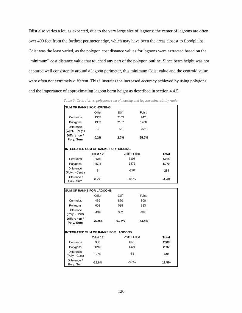
120
Fdist also varies a lot, as expected, due to the very large size of lagoons; the center of lagoons are often
over 400 feet from the furthest perimeter edge, which may have been the areas closest to floodplains.
Cdist was the least varied, as the polygon cost distance values for lagoons were extracted based on the
“minimum” cost distance value that touched any part of the polygon outline. Since berm height was not
captured well consistently around a lagoon perimeter, this minimum Cdist value and the centroid value
were often not extremely different. This illustrates the increased accuracy achieved by using polygons,
and the importance of approximating lagoon berm height as described in section 4.4.5.
Table 6: Centroids vs. polygons: sum of housing and lagoon vulnerability ranks.
Cdist Zdiff Fdist
Centroids 1305 2163 942
Polygons 1302 2107 1268
Difference
(Cent. - Poly.)3 56 -326
Difference /
Poly. Sum0.2% 2.7% -25.7%
Cdist * 2 Total
Centroids 2610 5715
Polygons 2604 5979
Difference
(Poly. - Cent.)6 -264
Difference /
Poly. Sum0.2% -4.4%
Cdist Zdiff Fdist
Centroids 469 870 500
Polygons 608 538 883
Difference
(Poly - Cent)-139 332 -383
Difference /
Poly. Sum-22.9% 61.7% -43.4%
Cdist * 2 Total
Centroids 938 2308
Polygons 1216 2637
Difference
(Poly - Cent)-278 329
Difference /
Poly. Sum-22.9% 12.5%
SUM OF RANKS FOR HOUSING
-8.0%
-3.6%
INTEGRATED SUM OF RANKS FOR LAGOONS
SUM OF RANKS FOR LAGOONS
INTEGRATED SUM OF RANKS FOR HOUSING
Zdiff + Fdist
3105
3375
-270
1421
Zdiff + Fdist
1370
-51
6 CONCLUSIONS
6.1 Assumptions and Limitations of Methods and Data
A review of the buyout sites (Figure 25) reveals that 6 out of 11 sites with a rank of less than 9 are
located in the very flat coastal plains where Beaufort, Hyde and Washington Counties meet, just to the
east of the Suffolk Scarp. FEMA’s estimated 100-year floodplains were actually quite far (2 to 7 km)
from some of these locations. However, they must have been flooded or otherwise damaged during
Hurricane Floyd due to their participation in the buyout program—all bids for the program were
extensively reviewed by the NC DENR and NC SCS; additional studies of flood hazard exposure were
performed when FEMA flood maps were deemed inaccurate or incomplete. The discrepancies in many of
the buyout site vulnerability rankings in this study may be related to the difficulties of FEMA contractors
to model the hydraulics of aggregate flooding and lagoonal retention effects of the Pamlico Sound (and
wider estuary system) after extreme, region-wide rainfall; or, perhaps, localized ponding effects occurred
which are also very difficult to model (NRC, 2009). This very large vulnerability rank discrepancy,
among what would have generally been expected to be the most vulnerable of all sites, suggests that many
other active and former farm sites are likely more vulnerable than indicated by these results.
A study of Hurricane Floyd’s flooding impact on hog farms by Wing et al. (2002) also
encountered significant discrepancies between expected vulnerability and model results. Their estimated
inundation area did not intersect a large number of lagoon sites that were confirmed by the NC Division
of Water Quality inspectors to be breached or flooded from Floyd. Their results indicated 237 total swine
farms were within the estimated Floyd flooding extent, but only 20 out of 46 sites with breached or
flooded lagoons were included in this count. Their flood extent was likely not highly accurate due to the
nature of its source data being synthetic aperture radar satellite imagery (unknown resolution) captured
over a week after Floyd hit. They also noted the limitations of using only the available permit points to
represent these very large farm sites as another likely source of error.

122
Although 195 expired sites were found in this study, including 31 lagoon buyout sites, there may
yet be more farms that were active before Floyd that were not included in this dataset. Inactive sites
without permit information were mostly discovered with the help of lagoon point data (these have no
descriptive attributes). However, approximately 22% of lagoons found that were confidently delineated as
swine waste lagoons did not have a corresponding lagoon point from this dataset. Therefore it seems
reasonable to expect still more inactive sites might have been included, given better information. It may
be possible to cross-check such information through NC DENR’s archived permit records, but this was
beyond the scope of this project.
The object-based polygon data created for all swine farm structures allowed for individual
structure vulnerability assessment, while also improving accuracy of overall site vulnerability assessment.
Assumptions that the FEMA 100-year floodplains are accurate in these rural agricultural areas are
challenged by the fact that so many lagoon buyout locations were not located in—or even near—100-year
floodplain boundaries.
6.2 Point vs. Polygon Conclusions
The differences in vulnerability analysis when using points versus polygons is most pronounced for
the lagoon structures. These lagoons are very large, and their berms are important measures of flood
protection that should be incorporated into flood vulnerability analyses. Using points for lagoons is not
adequate, and produces much less accurate results as shown in section 5.4. If lagoon berm height
information could be provided by the government or from farmers themselves, points may be more
viable. Without this information, polygons and high resolution elevation data are necessary to extract
approximate berm heights.
Housing structures, on the other hand, were much less varied in their vulnerability results when
using centroids instead of polygons. The majority of the differences were in the distance to nearest
floodplain (Fdist) rank, since these are quite large structures, and the furthest corner of a swine housing
unit may be the closest to a floodplain boundary. It seems reasonable, if a similar study were to be

123
conducted, to utilize points for swine housing or smaller structures, rather than polygons, in order to save
significant time in the delineation process.
6.3 Overall Conclusions
Despite the limitations of the 100-year floodplains or this study’s own methodology for
extrapolating vulnerability from these floodplain extents, it is clear that vulnerability of hog farms in the
study area significantly decreased after Hurricane Floyd. Aside from the 30 lagoon buyout program
participants known in the study area, the exact reason for the other 165 sites going inactive since 1998 is
not known. At least two-thirds of the lagoon buyout program applicants were turned away, primarily due
to limited funding. It is logical to expect that many farms were directly damaged or essentially destroyed
beyond economically feasible repairs from Floyd. Other flood impacts (e.g. loss of crops) may have
caused economic hardship for farmers after the disaster. Successive years of volatile pork market
fluctuations and fierce competition from contractors and integrators may also contribute to some of the
underlying motivations for many owners of these farms to exit the business, totally unrelated to flood
damages.
As discussed in section 2.3.9, the lagoon buyout program has been successful, but operated with
limited funding. Given more funding in the earlier phases, the program may have been able to bring
dozens of additional flood-vulnerable farms out of production. Many farms that were initially willing to
sell out in the program have since repaired structures and equipment and gone back into production. In
doing so, these sites have increased their value and decreased the likelihood that funding will be available
to make another significant phase of buyouts in the future, except perhaps in the case of another extreme
flooding event.
Environmentally-Superior Technologies (ESTs) for swine waste management have been in
development for 15 years, yet none have been widely implemented in the state. A state-led lagoon
conversion program has also had difficulty in getting many swine waste lagoons to be converted to EST
systems despite significant financial support from the state. It is clear that EST technology is still

124
complicated and expensive to implement. Perhaps, as in the development of solar and wind-power
technologies, EST solutions will only advance with continued and increased forward-thinking investment
and state incentives, without immediate insurance of commercial profitability. However, even EST
solutions do not fundamentally change the problems of operating CAFOs in areas vulnerable to flooding.
Waste lagoon breaches and contamination are only one aspect of the many potential external effects of
swine CAFO flooding. Housing structures necessarily contain significant waste before they are flushed to
a lagoon, or an EST system. Pigs themselves may still be exposed to flood hazards within flood-
vulnerable housing structures, and if they were to drown their carcasses also become sources of water
contamination.
Although regulations in NC were eventually evolved for better control of pollution, a lack of
siting control during the major period of hog farm expansion in ENC left the burgeoning industry in a
vulnerable state to flooding by 1999. A lack of any retroactive effects from newer legislation did not seem
to create any meaningful reform of the existing industry in terms of flood vulnerability. Hurricane Floyd
performed that role instead. In the aftermath of Floyd, however, the state’s lagoon buyout program did
have significant success in reducing the number of flood-vulnerable farms from continuing to operate.
Yet, this study finds that many active swine farm structures still remain very vulnerable to flooding to this
day.
Given more time and resources, it would have been interesting to compare relative vulnerability
of swine farm structures to other waste management structures, such as human wastewater treatment
plants and septic systems, which were also heavily impacted in many places in ENC after Floyd; or
poultry CAFOs, which are far less regulated than swine farms, yet also store incredible amounts of animal
manure and incorporate it into the surrounding agricultural landscape. Further study would benefit from
understanding how agricultural operations with such capital-intensive structues are (or are not) insured for
flood protection by private companies, and what kind of studies insurance companies might perform to
determine flood risk and insurance rates. This study created confident first-order analysis of flood
vulnerability over a very large region, but further research might focus on more local areas from a

125
hydrologic perspective, and how more accurate bio-physical flood exposure analysis can be integrated
into more comprehensive flood vulnerability conceptions that consider potential environmental and
human health impacts if certain sites were to be impacted by extreme floodwaters. These are important
issues of environmental justice (EJ) that are increasingly being studied in the field of geography and in
other academic fields. The methodology presented in this study may be a valuable tool to attain data for
use in future research for flood vulnerability of animal production industries within the EJ framework.
These methods can be applied to other regions performing similar swine CAFO production, and may be
especially applicable to other kinds of animal production or industry with high potential for
environmental impacts, such as aquaculture, hazardous waste storage, or even human wastewater
treatment facilities.

REFERENCES
Bagli, S., Geneletti, D., & Orsi, F. (2011). Routeing of power lines through least-cost path analysis and multicriteria
evaluation to minimise environmental impacts. Environmental Impact Assessment Review, 31(3), 234–239.
Retrieved from http://www.sciencedirect.com/science/article/pii/S0195925510001393
Bales, J. D. (2003). Effects of hurricane floyd inland flooding, September–October 1999, on tributaries to Pamlico
Sound, North Carolina. Estuaries, 26(5), 1319–1328. http://doi.org/10.1007/BF02803634
Bales, J. D., & Childress, C. J. O. (1996). Aftermath of Hurricane Fran in North Carolina—Preliminary data on
flooding and water quality: USGS Open-File Report 96-499.
Bales, J. D., Oblinger, C. J., & Sallenger, A. H. J. (2000). Two Months of Flooding in Eastern North Carolina,
September–October 1999: USGS Water-Resources Investigations Report 00-4094.
Barker, J. C. (1996). Lagoon Design and Management For Livestock Waste Treatment and Storage (No. EBAE 103-
83). Raleigh, NC: North Carolina Cooperative Extension Service. Retrieved from
http://www.bae.ncsu.edu/extension/ext-publications/waste/animal/ebae-103-83-lagoon-design-barker.pdf
Braun, J. (1998). Inside the Industry from a Family Hog Farmer. In K. M. Thu & E. P. Durrenberger (Eds.), Pigs,
Profits, and Rural Communities (pp. 39–56). SUNY Press.
Brivio, P. A., Colombo, R., Maggi, M., & Tomasoni, R. (2002). Integration of remote sensing data and GIS for
accurate mapping of flooded areas. International Journal of Remote Sensing, 23(3), 429–441. Retrieved from
http://bit.ly/1LhPM39
Burkholder, J., Eggleston, D., Glasgow, H., Brownie, C., Reed, R., Janowitz, G., … Springer, J. (2004).
Comparative impacts of two major hurricane seasons on the Neuse River and western Pamlico Sound
ecosystems. Proceedings of the National Academy of Sciences of the United States of America, 101(25), 9291–
9296. http://doi.org/10.1073/pnas.0306842101
Burns, J. D. (1996). Eight Million Little Pigs—A Cautionary Tale: Statutory and Regulatory Responses to
Concentrated Hog Farming. The Wake Forest Law Review, 31, 851.
Cutter, S. L. (1996). Vulnerability to environmental hazards. Progress in Human Geography, 20(4), 529–539.
Retrieved from http://webra.cas.sc.edu/hvri/docs/progress_human_geography.pdf
CWFNC. (2015). Your Drinking Water. Retrieved May 20, 2015, from http://www.cwfnc.org/community-
news/your-drinking-water/#Well
CWMTF. (2008). Update on The Program to Acquire Conservation Easements on Swine Operations in the 100-year
Floodplain. Clean Water Management Trust Fund.
Day, C. (2015, September 17). WOTUS: A mucky mess. Nationalhogfarmer.com. Retrieved from
http://nationalhogfarmer.com/environment/wotus-mucky-mess
DENR. (n.d.). Update to CWMTF Trustees on the Program to Acquire Conservation Easements On Swine
Operations in the 100-year Floodplain. Unpublished document.
Dhuyvetter, K. C., Tonsor, G. T., Tokach, M. D., Dritz, S. S., & Derouchey, J. (2014a). Farrow-to-Finish Swine
Cost-Return Budget.
Dhuyvetter, K. C., Tonsor, G. T., Tokach, M. D., Dritz, S. S., & Derouchey, J. (2014b). Swine Wean-to-Finish Cost-

127
Return Budget.
Doering, C. (2014, January 7). Smithfield urges farmers to end use of gestation crates. USA Today. Retrieved from
http://www.usatoday.com/story/news/nation/2014/01/07/hog-crates-ban/4362353/
Douglas, D. H. (1994). Least-cost path in GIS using an accumulated cost surface and slope lines. Cartographica,
31(3), 37.
Dow, K. (1992). Exploring differences in our common future(s): the meaning of vulnerability to global
environmental change. Geoforum, 23(3), 417–436. Retrieved from
http://www.sciencedirect.com.jproxy.lib.ecu.edu/science/article/pii/0016718592900526
Drustrup, B. (2014). Nutrients in Iowa’s Waters. Retrieved from http://igwa.org/docs.ashx?id=190084
Durrenberger, E. P., & Thu, K. M. (1996). The Industrialization of Swine Production in the United States: An
Overview. Culture & Agricullture, 18(1), 19–22.
Easley, M. (2000, July 25). Smithfield Agreement. Retrieved from
http://www.cals.ncsu.edu/waste_mgt/smithfield_projects/agreement.pdf
EDF. (2000, July 25). Environmentalists Applaud Action Requiring Smithfield Foods To Eliminate NC Hog
Lagoons. Environmental Defense Fund. Retrieved from https://www.edf.org/news/environmentalists-applaud-
action-requiring-smithfield-foods-eliminate-nc-hog-lagoons
Edwards, B., & Ladd, A. E. (2000). Environmental Justice, Swine Production and Farm Loss in North Carolina.
Sociological Spectrum, 20(3), 263–290.
Eller, D. (2015, March 17). DNR leader: Enforcement Difficult if Water Lawsuit is Successful. Des Moines
Register. Des Moines. Retrieved from
http://www.desmoinesregister.com/story/money/agriculture/2015/03/17/gipp-enforcement-difficult-water-suit-
successful/24932691/
Essig, M. (2015). Lesser Beasts: A Snout-to-Tail History of the Humble Pig. Basic Books.
Fernandez, L. (2015). PEDv in the US, two years later. Retrieved from http://www.wattagnet.com/articles/22236-
pedv-in-the-us-two-years-later
Flanders, A. (2014). Input Costs Trends for Arkansas Field Crops , 2008-2014. Northeast Research and Extension
Center. Keiser, AR. Retrieved from http://www.uaex.edu/farm-ranch/economics-marketing/farm-
planning/FlandersInputCosts_Augt2014.pdf
Frey, M., Hopper, R., & Fredregill, A. (2000). Spills and Kills: Manure Pollution and America’s Livestock Feedlots.
Clean Water Network.
Furuseth, O. J. (1997). Restructuring of Hog Farming in North Carolina: Explosion and Implosion. The Professional
Geographer, 49(4), 391–403. http://doi.org/10.1111/0033-0124.00086
Galaviz-villa, I., Martínez-dávila, J. P., & Pérez-vázquez, A. (2010). Agricultural Contamination of Subterranean
Water with Nitrates and Nitrites: An Environmental and Public Health Problem. Journal of Agricultural
Science, 2(2), 17–30.
Genoways, T. (2014). The Chain: Farm, Factory, and the Fate of Our Food. Harper.
Goodchild, M. F., Yuan, M., & Cova, T. J. (2007). Towards a general theory of geographic representation in GIS.
International Journal of Geographical Information Science, 21(3), 239–260. Retrieved from

128
http://www.tandfonline.com/doi/abs/10.1080/13658810600965271
Grey, M. A. (1998). Meatpacking in Storm Lake, Iowa: A Community in Transition. In K. M. Thu & E. P.
Durrenberger (Eds.), Pigs, Profits, and Rural Communities (pp. 57–70). SUNY Press.
Harden, S. L., & Spruill, T. B. (2004). Ionic Composition and Nitrate in Drainage water From Fileds Fertilized with
Different Nitrogen Sources, Middle Swamp watershed, North Carolina, August 2000-August 2001 (No. 2004-
5123 Scientific Investigations Report). USGS.
Harper, A. F., DeRouchey, J. M., Glanville, T. D., Meeker, D. L., & Straw, B. E. (2008). Swine Carcass Disposal
Options for Routine and Catastrophic Mortality. Council for Agricultural Science and Technology (CAST).
Issue Paper 39.
Henderson, B. (2015, January 1). NC hog farm neighbors seek court help to stop the stink. The News & Observer of
Raleigh. Retrieved from http://www.newsobserver.com/news/local/article10209392.html
Huffman, R. L. (1999). Groundwater Impacts of Lagoons. Raleigh, NC.
Huffman, R. L. (2004). Seepage Evaluation of Older Swine Lagoons in North Carolina. Transactions of the ASAE,
47(January 1993), 1507–1512. Retrieved from http://www.prairieswine.com/pdf/3112.pdf
Ikerd, J. (1998). Sustainable Agriculture, Rural Economic Development, and Large-Scale Swine Production. In K.
M. Thu & E. P. Durrenberger (Eds.), Pigs, Profits, and Rural Communities (p. 157–). SUNY Press.
Jackson, L. L. (1998). Large-Scale Swine Production and Water Quality. In K. M. Thu & E. P. Durrenberger (Eds.),
Pigs, Profits, and Rural Communities (pp. 103–122). SUNY Press.
Jackson, L. L., Hallberg, G., Huffman, R. L., Keeney, D., Lanyon, L. E., Lynch, N., & Schulte, D. D. (1996). Water
Quality. In K. Thu & L. L. Jackson (Eds.), Understanding the impacts of large-scale swine production:
Proceedings from an Interdisciplinary Scientific Workshop (pp. 10–45). Iowa.
Jess Clark. (n.d.). Community. Retrieved from http://wholehognc.org/community.html
Jones, D. D., Koelsch, R. K., Mukhtar, S., Sheffield, R., & Worley, J. W. (2006). Closure of Earthern Manure
Structures (Including Basins, Holding Ponds and Lagoons). In Conference Presentations and White Papers:
Biological Systems Engineering. Retrieved from
http://digitalcommons.unl.edu/cgi/viewcontent.cgi?article=1003&context=biosysengpres
Key, N., & McBride, W. (2007). The Changing Economics of U.S. Hog Production. US Department of Agriculture,
Economic Research Service, Economic Research Report Number 52.
Knutson, T. R., McBride, J. L., Chan, J., Emanuel, K., Holland, G., Landsea, C., … Sugi, M. (2010). Tropical
cyclones and climate change. Nature Geoscience, 3(3), 157–163. Retrieved from
http://www.nature.com/ngeo/journal/v3/n3/abs/ngeo779.html
Krause, K. . (1983). Corporate Farming: Importance, Incentives, and State Restrictions. US Department of
Agriculture.
Ladd, A. E., & Edwards, B. (2002). Corporate Swine and Capitalist Pigs: a Decade of Environmental Injustice and
Protest in North Carolina. Social Justice, 29(3), 26–47. Retrieved from
http://www.questia.com/PM.qst?a=o&se=gglsc&d=5000640793
Lowe, P. (2014, September 29). Everything But The Squeal: How The Hog Industry Cuts Food Waste. NPR.
Retrieved from http://www.npr.org/sections/thesalt/2014/09/29/351495505/everything-but-the-squeal-how-
the-hog-industry-cuts-food-waste

129
Mallinson, D. J., Culver, S. J., Riggs, S. R., Walsh, J. P., Ames, D., & Smith, C. W. (2008). Past, present and future
inlets of the Outer Banks barrier islands, North Carolina. East Carolina University Printing Press.
Greenville, NC. Retrieved from
https://www.ecu.edu/icsp/ICSP/Reports_files/PastPresentAndFutureInletsDec2008.pdf
Mankiw, N. G. (2008). Principles of Microeconomics (5th ed.). South-Western Cengage Learning.
Martinez, S. W. (1999). Vertical Coordination in the Pork and Broiler Industries: Implications for Pork and
Chicken Products. USDA Agricultural Economic Report No. 777.
McKenna, M. (2013). “Pig MRSA” Carried by Workers from North Carolina Intensive Hog Farms. Retrieved from
http://www.wired.com/2013/07/st398-nc-hogs/
Meinch, T. (2015, March 11). Water Works Votes to Sue 3 Iowa Counties over Nitrates. Des Moines Register. Des
Moines. Retrieved from http://www.desmoinesregister.com/story/money/agriculture/2015/03/10/utility-
consider-pursuing-water-quality-suit/24728999/
Melvin, S., Bundy, D., Casey, K., Miner, R., Schiffinan, S. S., & Sweeten, J. (1996). Air Quality. In K. Thu & L. L.
Jackson (Eds.), Understanding the impacts of large-scale swine production: Proceedings from an
Interdisciplinary Scientific Workshop (pp. 46–68). Iowa.
Meng, X. J., Lindsay, D. S., & Sriranganathan, N. (2009). Wild boars as sources for infectious diseases in livestock
and humans. Philosophical Transactions of the Royal Society of London. Series B, Biological Sciences,
364(1530), 2697–2707. http://doi.org/10.1098/rstb.2009.0086
Merz, B., Thieken, A. H., & Gocht, M. (2007). Flood risk mapping at the local scale: concepts and challenges. In S.
Begum, M. J. F. Stive, & J. W. Hall (Eds.), Flood risk management in Europe (pp. 231–251). Springer
Netherlands. Retrieved from
https://www.researchgate.net/profile/Annegret_Thieken/publication/226038430_Flood_Risk_Mapping_At_Th
e_Local_Scale_Concepts_and_Challenges/links/0deec533af04ec4cc2000000.pdf
Messner, F., & Meyer, V. (2006). Flood damage, vulnerability and risk perception – challenges for flood damage
research. In Flood Risk Management: Hazards, Vulnerability and Mitigation Measures (pp. 149–167).
http://doi.org/10.1007/978-1-4020-4598-1
Mikkelsen, R. L. (1995). Swine Waste Disposal Dilemma: A Case Study, 24(2), 169–173.
Mikkelsen, R. L., Power, J. F., Dick, W. A., Kashmanian, R. M., Sims, J. T., Wright, R. J., … Bezdicek, D. (2000).
Beneficial use of swine by-products: opportunities for the future. (pp. 451–480). Soil Science Society of
America Inc. Retrieved from
http://www.cabdirect.org/abstracts/20003037615.html;jsessionid=AA3C692F42F61774B4D76F869786E72D
Morgan, R. (1998). Legal and Political Injustices of Industrial Swine Production in North Carolina. In K. M. Thu &
E. P. Durrenberger (Eds.), Pigs, Profits, and Rural Communities (pp. 121–144). SUNY Press.
Morrison, J. M. (1998). The Poultry Industry: A View of the Swine Industry’s Future? In K. M. Thu & E. P.
Durrenberger (Eds.), Pigs, Profits, and Rural Communities (pp. 145–154). SUNY Press.
NCDACS. (n.d.). NC Department of Agriculture and Consumer Services: Conservation Easement Viewer. Retrieved
January 10, 2015, from http://www.ncmhtd.com/soilwater/crep/
NCDENR. (2008). 2008 Interim report on the lagoon conversion program for innovative swine waste management
systems. Retrieved from
http://www.ncagr.gov/SWC/documents/ERC_2008_LCP_Report112508_attachments.pdf
130
NCDENR. (2009). Ninth Senate Bill (SB) 1217 Interagency Group Guidance Document. Retrieved from
http://www.ncagr.gov/SWC/tech/documents/9th_Guidance_Doc_100109.pdf
NCDWR. (2015). Animal Feeding Operations Active Permits: Updated 1-5-15. NC Division of Water Resources.
Retrieved from http://portal.ncdenr.org/web/wq/aps/afo/perm
NCFM. (2008). North Carolina Floodplain Management Quick Guide. Retrieved from
http://www.ncfloodmaps.com/pubdocs/nc_quick_guide_2008.pdf
NCFMP. (2008). North Carolina Floodplain Mapping Program: 2000 – 2008 Program Review. Retrieved from
http://www.ncfloodmaps.com/pubdocs/program_review/
NCFMP. (2014). North Carolina Floodplain Mapping Program FLOOD Geodatabase. Retrieved from
http://fris.nc.gov/fris_hardfiles/nc/hardfiles/file_s_hydramodel/nc_flood_gdb_design.zip
NCGA. Senate Bill 926: Swine Farm Odor Abatement Study (1993). Retrieved from
http://www.ncleg.net/Sessions/1993/Bills/Senate/PDF/S926v2.pdf
NCGA. House Bill 898: The Studies Act of 1995 (1995). Retrieved from
http://www.ncleg.net/Sessions/1995/Bills/House/PDF/H898v5.pdf
NCGA. Senate Bill 1080: Swine Farm Siting Act (1995). Retrieved from
http://www.ncleg.net/Sessions/1995/Bills/Senate/PDF/S1080v7.pdf
NCGA. Sentate Bill 974: Swine Waste Management Certification (1995). Retrieved from
http://www.ncleg.net/Sessions/1995/Bills/Senate/PDF/S974v7.pdf
NCGA. Senate Bill 1217: Iimplementation of Recommendations of the Blue Ribbon Study Commission on
Agricultural Waste (1996). Retrieved from
http://www.ncleg.net/Sessions/1995/Bills/Senate/PDF/S1217v5.pdf
NCGA. House Bill 515: Clean Water Responsibility Act (1997). Retrieved from
http://www.ncleg.net/Sessions/1997/Bills/House/PDF/H515v6.pdf
NCGA. House Bill 1480: Moratoria Exemptions and Clarifications and Swine Integrator Registration (1998).
Retrieved from http://www.ncleg.net/Sessions/1997/Bills/House/PDF/H1480v3.pdf
NCGA. Senate Bill 1465: An Acto to Codify and Make Permanent Swine Waste Management Performance
Standards (2007). Retrieved from http://www.ncleg.net/Sessions/2007/Bills/Senate/PDF/S1465v7.pdf
NCGA. (2012). House bill 819: An Act to Study and Modify Certain Coastal Management Policies. Retrieved from
http://www.ncleg.net/Sessions/2011/Bills/House/PDF/H819v6.pdf
NCGICC. (2008). State Geographic Information Consolidation Implementation Plan. NC Geographic Information
Coordinating Council. Retrieved from http://goo.gl/J1qoUI
NCGICC. (2010). Business Plan for Orthoimagery in North Carolina. NC Geographic Information Coordinating
Council. Retrieved from http://ncgicc.net/Portals/3/documents/OrthoImageryBusinessPlan_NC_20101029.pdf
NCMHTD. (2015). Google Earth WMS Services. Retrieved December 6, 2015, from
http://www.ncmhtd.com/ge_wms.aspx
NCSU. (2013). Development of Environmentally Superior Technologies for Swine Waste Management per
Agreements between the Attorney General of North Carolina, Smithfield Foods, Premium Standards Farms,
and Frontline Farmers. Retrieved from

131
http://www.cals.ncsu.edu/waste_mgt/smithfield_projects/smithfieldsite.htm
Neo, H., & Chen, L. H. (2009). Household income diversification and the production of local meat: the prospect of
small‐ scale pig farming in Southern Yunnan, China. Area, 41(3), 300–309.
Niman, N. H. (2008). Righteous Porkchop: Finding a Life and Good Food Beyond Factory Farms. New York, NY:
Haper.
Nowlin, M. (1997). Point Counter Point. Journal of Soil and Water Conservation (USA), 52(5), 314–319.
NRC. (2009). Mapping the Zone: Improving Flood Map Accuracy. The National Academies Press. Retrieved from
http://www.nap.edu/catalog.php?record_id=12573
O’Driscoll, M. A. (2012). The 1909 North Carolina Drainage Act and Agricultural Drainage Effects in Eastern
North Carolina. Journal of North Carolina Academy of Science, 128(3), 59–73. http://doi.org/10.7572/2167-
5880-128.3.59
Paerl, H. W., Bales, J. D., Ausley, L. W., Buzzelli, C. P., Crowder, L. B., Eby, L. A., … Ramus, J. S. (2001).
Ecosystem impacts of three sequential hurricanes (Dennis, Floyd, and Irene) on the United States’ largest
lagoonal estuary, Pamlico Sound, NC. Proceedings of the National Academy of Sciences of the United States
of America, 98(10), 5655–5660. http://doi.org/10.1073/pnas.101097398
Paerl, H. W., Pinckney, J., Fear, J. M., & Peierls, B. (1998). Ecosystem responses to internal and watershed organic
matter loading:consequences for hypoxia in the eutrophying Neuse River Estuary, North Carolina, USA.
Marine Ecology Progress Series, 166, 17–25. http://doi.org/10.3354/meps166017
Paerl, H. W., Valdes, L. M., Joyner, A. R., Peierls, B. L., Piehler, M. F., Riggs, S. R., … Luettich, R. a. (2006).
Ecological response to hurricane events in the Pamlico Sound system, North Carolina, and implications for
assessment and management in a regime of increased frequency. Estuaries and Coasts, 29(6), 1033–1045.
http://doi.org/10.1007/BF02798666
Palmer, D. (2013, September 6). U.S. approves purchase of Smithfield. Politico. Retrieved from
http://www.politico.com/story/2013/09/us-china-smithfield-096399
Paul, M. J., & Meyer, J. L. (2001). Streams in the urban landscape. Annual Review of Ecology and Systematics, 32,
333–365. Retrieved from https://www.floodplain.org/Paul_Meyer_Urban_Streams.pdf
Petty, A. M. (2013). Standing Their Ground: Small Farmers in North Carolina Since the Civil War. Oxford
University Press.
Phillips, L. (2012). US northeast coast is hotspot for rising sea levels. Nature.
http://doi.org/10.1038/nature.2012.10880
Pig International. (2005). Profiling China. Pig International, 35(1), 11–13.
Raposo, M. (2015, October 14). Murphy-Brown Faces New Legal Challenge after Ignoring Agreement to Clean Up
Hog Farm Contamination. Waterkeeper.org. Retrieved from http://waterkeeper.org/2015/10/14/murphy-
brown-faces-new-legal-challenge-after-ignoring-agreement-to-clean-up-hog-farm-contamination/
RENCI. (2012). Storms to Life: Hurricane Floyd Economic Impact. Retrieved December 6, 2015, from
https://www.ecu.edu/renci/StormsToLife/Floyd/economic.html
Rinsky, J. L., Nadimpalli, M., Wing, S., Hall, D., Baron, D., Price, L. B., … Heaney, C. D. (2013). Livestock-
Associated Methicillin and Multidrug Resistant Staphylococcus aureus Is Present among Industrial, Not
Antibiotic-Free Livestock Operation Workers in North Carolina. PLoS ONE, 8(7). Retrieved from

132
http://journals.plos.org/plosone/article?id=10.1371/journal.pone.0067641
Rivin, G. (2015, August 18). Clock Ticking as EPA Prepares Response Over Hog Pollution. North Carolina Health
News. Retrieved from http://www.northcarolinahealthnews.org/2015/08/18/clock-ticking-as-epa-prepares-
response-over-hog-pollution/
Schmidt, C. W. (2000). Lessons from the flood: Will Floyd change livestock farming? Environmental Health
Perspectives. http://doi.org/10.1289/ehp.108-a74
Schneider, M. (2014). Developing the meat grab. The Journal of Peasant Studies, 41(4), 613–633.
Schroeter, J. R., Azzam, A. M., & Aiken, J. D. (2006). Anti-corporate farming laws and industry structure: the case
of cattle feeding. The American Journal of Agricultural Economics, 88(4), 1000–1014.
Singh, S. (2015, August 18). China Culling 100 Million Hogs Means Record Pork Imports. Www.bloomberg.com.
Retrieved from http://www.bloomberg.com/news/articles/2015-08-18/china-culling-100-million-hogs-means-
record-pork-imports
Smothers, R. (1995, June 30). Spill Puts a Spotlight On a Powerful Industry. The New York Times. Retrieved from
http://www.nytimes.com/1995/06/30/us/spill-puts-a-spotlight-on-a-powerful-industry.html
Staff, C. J. (2005, October 6). Hog-Farm Buyout List Grows. Carolina Journal Online. Retrieved from
http://www.carolinajournal.com/issues/display_story.html?id=2829
Stith, P., & Warrick, J. (1995, February 22). Murphy’s Law: For Murphy, good government means good business.
The News & Observer of Raleigh. Raleigh, NC. Retrieved from http://www.pulitzer.org/archives/5897
Stith, P., Warrick, J., & Sill, M. (1996). Pulitzer Prize Archives for Boss Hog: The power of pork. Retrieved from
http://www.pulitzer.org/archives/5892
Strock, J. S., Kleinman, P. J., King, K. W., & Delgado, J. A. (2010). Drainage water management for water quality
protection. Journal of Soil and Water Conservation (USA), 65(6), 131A–136A.
Strom, S. (2014, July 4). Virus Plagues the Pork Industry, and Environmentalists. New York Times. Retrieved from
http://www.nytimes.com/2014/07/05/business/PEDv-plagues-the-pork-industry-and-
environmentalists.html?_r=0
Strom, S. (2015, May 22). Walmart Pushes for Improved Animal Welfare. The New York Times. Retrieved from
http://www.nytimes.com/2015/05/23/business/walmart-pushes-for-improved-animal-welfare.html
Sylves, R. (2008). Disaster Policy and Politics: Emergency Management and Homeland Security (1st ed.). CQ
Press.
Tatum, S. (1910). Reclamation and drainage. Annals of the American Academy of Political and Social Science,
35(1), 77–80.
Tester, P. a., Varnam, S. M., Culver, M. E., Eslinger, D. L., Stumpf, R. P., Swift, R. N., … Litaker, R. W. (2003).
Airborne detection of ecosystem responses to an extreme event: Phytoplankton displacement and abundance
after hurricane induced flooding in the Pamlico-Albemarle Sound system, North Carolina. Estuaries, 26(5),
1353–1364. http://doi.org/10.1007/BF02803637
Thu, K. M., & Durrenberger, E. P. (1994). North Carolina’s hog industry: The rest of the story. Culture &
Agricullture, 14(49), 20–23.
Todd, J. L. (1996). Environmental Law: The Clean Water Act—Understanding When a Concentrated Animal

133
Feeding Operation Should Obtain an NPDES Permit. Oklahoma Law Review, 49, 481.
U.S. EPA. (2007). Nitrates and Nitrites: TEACH Chemical Summary.
U.S. EPA. (2012). The Clean Water Act: Protecting and Restoring our Nation’s Waters. Retrieved from
http://water.epa.gov/action/cleanwater40/cwa101.cfm
Upton, J. (2015, April 29). How farmers can benefit from cap and trade. Retrieved May 5, 2015, from
http://www.greenbiz.com/article/how-farmers-can-benefit-cap-and-trade
US Pork Checkoff. (2014). Pork Quick Facts - Stats. Retrieved from
https://d3fns0a45gcg1a.cloudfront.net/sites/all/files/documents/Pork_Quickfacts_Stats_2014.pdf
USDA. (2009). Chapter 10: Agricultural Waste Management System Component Design. Agricultural Waste
Management Field Handbook. Retrieved from ftp://ftp.wcc.nrcs.usda.gov/wntsc/AWM/handbook/ch10.pdf
USDA. (2015). US Agricultural Census. Retrieved December 6, 2015, from http://www.agcensus.usda.gov/
USFDA. (2015). Veterinary Feed Directive (VFD). Retrieved from
http://www.fda.gov/AnimalVeterinary/DevelopmentApprovalProcess/ucm071807.htm
USGS. (n.d.). The National Map Viewer. Retrieved January 10, 2015, from http://viewer.nationalmap.gov/viewer/
Warrick, J. (1995, June 23). Hog-waste spill fouls land, river in Onslow. The News & Observer of Raleigh. Raleigh,
NC. Retrieved from http://www.learnnc.org/lp/editions/nchist-recent/6172
Warrick, J., & Leavenworth, S. (1995, June 29). Waste spill revives hog legislation. House looks again at farm
regulations. The News & Observer of Raleigh. Raleigh, NC. Retrieved from
http://www.learnnc.org/lp/editions/nchist-recent/6271
Warrick, J., & Stith, P. (1995a, February 19). New studies show that lagoons are leaking. The News & Observer of
Raleigh. Retrieved from http://www.pulitzer.org/archives/5893
Warrick, J., & Stith, P. (1995b, February 21). Corporate takeover. The News & Observer of Raleigh. Retrieved from
http://www.pulitzer.org/archives/5896
Waterkeeper Alliance. (2014). Letter to NC Department of Agriculture Commissioner Steve Troxler RE: Swine
Mortality Disposal Associated with the PED Outbreak. Waterkeeper Alliance. Retrieved from
http://waterkeeper.org/cms/assets/uploads/2014/02/Letter-to-Troxler-2-27-14-.pdf
Webster, P. J., Holland, G. J., Curry, J. A., & Chang, H.-R. (2005). Changes in Tropical Cyclone Number, Duration,
and Intensity in a Warming Environment. Science, 309(5742), 1844–1846. Retrieved from
http://www.sciencemag.org/content/309/5742/1844.short
Williams, M. (2013). Evaluation of Generation 3 Treatment Technology for Swine Waste. North Carolina State
University Animimal and Poultry Waste Management Center. Retrieved from
http://www.bae.ncsu.edu/topic/waste-mgmt-center/CWMTF-report/CWMTF-Report-generation-2013.pdf
Wing, S., Freedman, S., & Band, L. (2002). The potential impact of flooding on confined animal feeding operations
in eastern North Carolina. Environmental Health Perspectives, 110(4), 387–391.
Yu, C., Lee, J. A. Y., & Munro-Stasiuk, M. J. (2003). Extensions to least-cost path algorithms for roadway planning.
International Journal of Geographical Information Science, 17(4), 361–376. Retrieved from
http://bit.ly/1GF3J9h