In�ation and Interest Rates with Endogenous Market Segmentation

Aubhik Khan

The Ohio State University

Julia K. Thomas�

The Ohio State Universityand NBER

September 2009

ABSTRACT

We examine a monetary economy wherein endogenous asset market segmentation permits the extentof household participation in open market operations to smoothly vary with changes in aggregateconditions. While we impose no stickiness at the microeconomic level in either prices or portfolioadjustment, we �nd that our �exible asset market segmentation can deliver gradual adjustment inthe aggregate price level following a monetary shock and thus persistent non-neutralities.

In our model economy, households incur �xed transactions costs when exchanging bonds and moneyand, as a result, carry money balances in excess of current spending to limit the frequency of suchtrades. As only a fraction of households choose to actively trade bonds and money at any giventime, the market is endogenously segmented. Moreover, because our households have the ability toalter the timing of their trading activities, the extent of market segmentation varies over time inresponse to real and nominal shocks. We show that this added �exibility can substantially reinforceboth sluggishness in aggregate price adjustment, and the persistence of liquidity e¤ects in real andnominal interest rates, relative to models with exogenously segmented asset markets.

�Thomas gratefully acknowledges research support from the Alfred P. Sloan Foundation and the NationalScience Foundation (grant #0318163).

1 Introduction

There is a wealth of empirical research documenting not only the co-movement of real andnominal series at higher frequencies, but what is widely accepted as evidence of persistent responsesin real variables following nominal disturbances. We study such co-movements using a monetarymodel wherein households face �xed costs of transferring wealth between interest-bearing assetsand money. As a result of these transactions costs, households infrequently access their interestincome and carry money balances in excess of current spending, and participation in asset marketsis endogenously segmented. As is well known, market segmentation implies that open marketoperations can have real e¤ects, because they directly involve only a subset of households. Thispaper establishes that, when market segmentation is endogenized in a setting where householdshold inventories of money, changes in the fraction of households participating in asset markets canadd considerable persistence to movements in both nominal and real variables.

Our work builds on an important literature that studies monetary policy in models with ex-ogenously segmented markets.1 As in the work of Grossman and Weiss (1983), Rotemberg (1984),and Alvarez, Atkeson and Edmond (2003), households in our model economy only periodicallyaccess the market for interest-bearing assets (broadly interpreted as markets for relatively high-yield assets) and they carry inventories of money (interpreted to include relatively low yield liquidassets). Nonetheless, our model is closest in spirit to the endogenous segmentation model of Al-varez, Atkeson and Kehoe (2002), in that heterogeneous households actively choose when to adjusttheir portfolios of bonds and money.2 Our model is distinguished relative to theirs by a nontrivialdistribution of money that evolves across periods, as most households do not exhaust their moneybalances with their current consumption expenditures. As in Alvarez, Atkeson and Edmond (2003),our household spending rates (ratios of the value of current consumption to money holdings) arelowest among households that have recently transferred wealth held as bonds into money, and theyrise with the time since such a transfer has occurred. In such an environment, a transitory shock tomoney growth changes the distribution of money holding across households with di¤erent spendingrates, which can, in turn, generate persistent movements in in�ation rates.

Unlike exogenous segmentation environments such as Alvarez, Atkeson and Edmond (2003), theextent of market segmentation varies over time in our model economy, as the fraction of householdschoosing to participate in the asset markets responds to changes in the economy�s state. Moreover,in contrast to the endogenous segmentation model of Chiu (2005), our allowance for idiosyncraticdi¤erences across households implies that this fraction remains nontrivial over time, as does thedistribution of money. This distinction has important implications for the propagation of nominaldisturbances. Following an open market operation, endogenous changes in the timing of households�active participation in asset markets can gradualize aggregate price adjustment relative to that in amodel with exogenous market segmentation. Furthermore, such changes can substantially increasethe persistence of liquidity e¤ects in both real and nominal interest rates.3

Endogenizing access to the asset market, and thus allowing for movements in the fraction of

1See Alvarez, Lucas and Weber (2001) and the references therein.2Alvarez, Atkeson and Kehoe (2002) build on the work of Chatterjee and Corbae (1991) who study an economy

where some households choose to pay a �xed cost to trade bonds.3One exception to this is the exogenous segmentation model of Williamson (2005), where households are perma-

nently divided into groups with and without access to the asset markets. There, the assumption that households with(without) such access prefer to trade among themselves in the goods markets delivers a second type of segmentationthat can lead to persistent liquidity e¤ects.

1

households actively adjusting their nominal balances at any time, implies larger movements in indi-vidual households�spending rates following a shock to the money supply. When transactions costsare high, and thus the mean time between active trades is long, households tend to hold relativelylarge inventories of money and have lower average spending rates. If, in addition, the maximumtime between trades is signi�cantly longer than is the mean time, households on average return tothe asset markets with substantial remaining balances. We �nd that, in such circumstances, thepersistence in in�ation that is implied by the exogenous segmentation model is reduced, as house-holds not currently participating in the asset markets sharply raise their spending rates followingan open market operation. Conversely, when the mean time between asset market trades is not aslong, so that households have higher average spending rates (or when the mean and maximum timesbetween such trades are similar, so that households on average return to the bond market withlittle remaining money), endogenous changes in the distribution of households increase persistencein the in�ation response beyond that in the exogenous segmentation model and, moreover, lead topersistent changes in interest rates.

As in the many studies in monetary economics that have preceded us, several empirical relation-ships involving money, interest rates and prices motivate our work. First, short-term real interestrates are negatively correlated with expected in�ation. Barr and Campbell provide direct evidencefor this using U.K. data involving in�ation-indexed bonds. Second, VAR studies consistently havefound evidence of liquidity e¤ects; expansionary open market operations appear to reduce short-term nominal interest rates, at least in the short-run. (See, for example, Leeper, Sims, and Zha(1996) and Christiano, Eichenbaum, and Evans (1999).) Finally, the general price level appears toadjust slowly to nominal shocks. This �nding is widely supported by the VAR literature as, for ex-ample, in the studies of Leeper, Sims, and Zha (1996), Christiano, Eichenbaum, and Evans (1999),and Uhlig (2004). Moreover, King and Watson (1996) show that, at business cycle frequencies,the price level is positively correlated with lagged real output. Additional evidence for the slowadjustment of the price level, discussed in Alvarez, Atkeson and Edmond (2003), is provided by thepattern of short-term movements seen between the ratio of money to consumption and velocity.The correlation between the ratio of money (M2) to consumption (PCE) and the correspondingmeasure of velocity is �0:89 for HP-�ltered monthly data.

The most common theoretical approach to addressing this empirical evidence involves modelswhere nominal prices are sticky at the �rm level. While there are several open issues involvingthe viability of models with sticky prices, we discuss one that directly motivates our work. Intheir recent paper, Dotsey and King (2005) resolve a long-standing issue for this literature bydeveloping an (S,s) model of nominal price setting that is consistent with empirical estimates of thepersistence in in�ation. In the process, they discover that their model predicts a rise in short-termnominal interest rates following a persistent shock to money growth rates. The state-of-the-artmicro-founded menu cost model cannot address the liquidity e¤ect described by Milton Friedman(1968), �The initial impact of increasing the quantity of money at a faster rate than it has beenincreasing is to make interest rates lower for a time than they would otherwise have been.�Whetheror not we choose to view this as a critical shortcoming of the paradigm, there is a more substantivedisagreement between Friedman�s view of the real e¤ects of monetary policy and that underlyingsticky price models. Friedman viewed changes in the velocity of money as central in determiningthe mechanics of movements in output, employment and prices following an expansionary openmarket operation. Consider his testimony to the House of Commons Select Committee in 1979; �...the initial e¤ect of a change in monetary growth is an o¤setting movement in velocity, followed by

2

changes in the growth of spending initially manifested in output and employment, and only later inin�ation.� (Friedman, 1980).4 This view is �rmly rejected by sticky price models where the velocityof money, and indeed real balances themselves, are almost entirely irrelevant to the predictions ofthe model.

Changes in velocity are at the heart of the short-term nonneutrality exhibited by models withsegmented assets markets. Moreover, the endogenous segmentation model of Alvarez, Atkesonand Kehoe (2002) succeeds in generating liquidity e¤ects and in reproducing the negative relationbetween real interest rates and anticipated in�ation. The Alvarez, Atkeson and Edmond (2003)inventory-theoretic model of money with exogenous segmentation separately delivers sluggish ad-justment of the price level, and hence persistent in�ation responses to nominal shocks. Drawingupon elements of each of these frameworks, we develop an endogenous segmentation model ofmoney that simultaneously succeeds with regard to both sets of regularities. Moreover, as men-tioned above, changes in the number of households choosing to exchange bonds and money cansubstantially reinforce the e¤ects of market segmentation. Following a transitory shock to themoney growth rate, such changes prolong responses in in�ation and the real interest rate. Whenshocks to money growth are persistent, they lead to far more sluggish price adjustment and morepersistent liquidity e¤ects in both nominal and real interest rates. Alternatively, when we examinereal shocks with monetary policy following a Taylor rule, our economy generates persistence inthe responses of in�ation and interest rates altogether absent under �xed market segmentation.Finally, in versions of our model with endogenous production, we �nd that persistent technologyshocks can lead to non-monotone responses in employment and output.

Finally, our paper o¤ers an independent theoretical contribution in formally establishing howthe results of Alvarez, Atkeson and Kehoe (2002) may be extended to a model where there are per-sistent di¤erences across households. Here, such extension is necessary, because cash-in-advanceconstraints do not always bind so that households carry inventories of money, thereby transmit-ting the e¤ects of temporary idiosyncratic di¤erences across periods. By assuming a full set ofstate-contingent nominal bonds that allow risk-sharing across households, we ensure that thesedi¤erences across households are persistent, but not permanent. Because households must pay�xed transactions costs to access their bond holdings, the presence of state-contingent bonds inour economy does not lead to full insurance; households that are ex-ante identical diverge overtime as idiosyncratic realizations of shocks drive di¤erences in their money and bond holdings.Nonetheless, we prove that, whenever a heterogeneous group of households enters the bond marketat the same time, all previous di¤erences among them are eliminated. As a result, our modeleconomy exhibits limited memory. Exploiting this property, we are able to apply the numericalapproach to solving generalized (S,s) models developed by King and Thomas (forthcoming) in asetting where the consumption and savings decisions of heterogeneous risk-averse households aredirectly in�uenced by nonconvex costs. While this approach has been applied previously in solvingmodels where risk-neutral production units face idiosyncratic �xed costs of adjusting their pricesor factors of production (as in Dotsey, King and Wolman (1999) and Thomas (2002)), this is toour knowledge the �rst application involving heterogeneity among households.

4We thank Ed Nelson for bringing this to our attention.

3

2 Model

We begin with an overview of the model. Thereafter, we proceed to a more formal descriptionof households�problems, followed by the description of a �nancial intermediary that sells house-holds claims contingent on both aggregate and individual states. Next, we show that there is anequivalent, but more tractable, representation of households�lifetime optimization problems, giventheir ability to purchase such individual-state-contingent bonds alongside the fact that they areex-ante identical. Proofs of all lemmas are provided in the appendix.

2.1 Overview

The model economy has three sets of agents: a unit measure of ex-ante identical households,a perfectly competitive �nancial intermediary, and a monetary authority. Each in�nitely-livedhousehold values consumption in every date of life, with period utility u(c), and it discounts futureutility with the constant discount factor �, where � 2 (0; 1). In each period, households receive acommon endowment, y. This endowment varies exogenously over time, as does the growth rate ofthe aggregate money supply, �. De�ning the date t realization of aggregate shocks as st = (yt; �t),we denote the history of aggregate shocks by st = (s1; : : : ; st), and the initial-period probabilitydensity over aggregate histories by g

�st�.

Households have two means of saving. First, they have access to a complete set of state-contingent nominal bonds. These are purchased from a �nancial intermediary described below,and are maintained in interest-bearing accounts that we will refer to as households� brokerageaccounts, following the language of Alvarez, Atkeson and Edmond (2003). Next, they also saveusing money, which they maintain in their bank accounts and use to conduct trades in the goodsmarket.5 Households have the opportunity to transfer assets between their two accounts at thestart of each period; this occurs after the realization of all current shocks, but prior to any tradingin the goods market. As such, it is expositionally convenient to refer to each period as consistingof two subperiods that we will term transfer-time and shopping-time, although nothing in theenvironment necessitates this approach.

There are three inter-related frictions leading households to maintain money in their bankaccounts. First, as in a standard cash-in-advance environment, households cannot consume theirown endowments. Each household consists of a worker and a shopper, and the worker must tradethe household endowment for money while the shopper is purchasing consumption goods. As aresult, the household receives the nominal value of its endowment, P (st)y

�st�, only at the end of

the period after current goods trade has ceased.6 We assume that these end-of-period nominalreceipts are deposited across their two accounts, with fraction � paid into bank accounts and theremainder into brokerage accounts. Second, as all trades in the goods market are conducted withmoney, each household�s consumption purchases are constrained by the bank account balance itholds when shopping-time begins.

Note that, absent other frictions, each household would, in every period, simply shift from itsbrokerage account into its bank account exactly the money needed to �nance current consumption

5When allowed to store money in their brokerage accounts, households never do so given positive nominal interestrates paid on bonds. Thus, we simplify the model�s exposition here by assuming that money is held only in bankaccounts and verify that nominal rates remain positive throughout our results.

6While this worker-shopper arrangement may appear stark in an endowment economy, it is less so if one envisionsthat each household�s endowment is one of a unit measure of di¤erentiated inputs that enter a consumption aggregatorwith identical weights to produce the single good consumed by all.

4

expenditure not covered by the bank account paycheck from the previous period. There is, however,a third friction that prevents this, leading households to deliberately carry money across periods;this is the assumption that they must pay �xed costs each time they transfer assets between theirtwo accounts. Given these �xed costs, households maintain stocks of money to limit the frequencyof their transfers, and they follow generalized (S,s) rules in managing their bank accounts.

Transfer costs are �xed in that they are independent of the size of the transfer; however,they vary over time and across households. Here, we subsume the idiosyncratic features thatdistinguish households directly in their �xed costs by assuming that each household draws itsown current transfer cost, �, from a time-invariant distribution H(�) at the start of each period.Because this cost draw in�uences a household�s decision of whether to undertake any transfer, andhence its current consumption and money savings, each household is distinguished by its historyof such draws, �t = (�1; : : : ; �t), with associated density h

��t�= h (�1) � � �h (�t). As will be seen

below, households are able to insure themselves in their brokerage accounts through the purchaseof nominal bonds contingent on both aggregate and individual exogenous states.

2.2 Households

At the start of any period, given date-event history�st; �t

�, a household�s brokerage account

assets include nominal bonds, B�st; �t

�, purchased in the previous period at price q

�st; �t

�, as well

as the fraction of its income from the previous period that is deposited there, (1��)P (st�1)y�st�1

�.

The remainder, the paycheck, �P (st�1)y�st�1

�, is deposited into the household�s bank account and

supplements its money savings there from the previous period, A�st�1; �t�1

�. Given this start of

period portfolio and its current �xed cost, the household begins the period by determining whetheror not to transfer assets across its two accounts. Denoting the household�s start-of-period bankbalance by M

�st�1; �t�1

�, where

M�st�1; �t�1

�� A

�st�1; �t�1

�+ �P (st�1)y

�st�1

�, (1)

the relevant features of this choice are summarized in the chart below.

brokerage account withdrawal shopping-time bank balancez�st; �t

�= 1 x

�st; �t

�+ P (st)�t M

�st�1; �t�1

�+ x

�st; �t

�z�st; �t

�= 0 0 M

�st�1; �t�1

�An active household is indicated by z

�st; �t

�= 1. In this case, the household selects a nonzero

nominal transfer x�st; �t

�from its brokerage account into its bank account and hasM

�st�1; �t�1

�+

x�st; �t

�available in its bank account at the start of the current shopping subperiod. Here, the

household�s current �xed cost applies, so P (st)�t is deducted from its nominal brokerage wealth.Alternatively, the household may choose to undertake no such transfer, setting z

�st; �t

�= 0 and

remaining inactive. In that case, it enters into the shopping subperiod with no change to itsstart-of-period bank and brokerage account balances.

Each household chooses its state-contingent plan for the timing and size of its account transfers(z�st; �t

�and x

�st; �t

�), and its bond purchases, money savings and consumption (B

�st; st+1; �

t; �t+1�,

A�st; �t

�and c

�st; �t

�), to maximize its expected discounted lifetime utility,

1Xt=1

�t�1Zst

Z�t

u�c(st; �t)

�h��t�g�st�d�tdst, (2)

5

subject to the sequence of constraints in (3) - (6).

B�st; �t

�+ (1� �)P

�st�1

�y�st�1

��hx�st; �t

�+ P

�st��t

iz�st; �t

�(3)

+

Zst+1

Z�t+1

q�st; st+1; �t+1

�B�st; st+1; �

t; �t+1�dst+1d�t+1

M�st�1; �t�1

�+ x

�st; �t

�z�st; �t

�� P

�st�c�st; �t

�+A

�st; �t

�(4)

A�st; �t

�+ �P (st)y

�st�� M

�st; �t

�(5)

A�st; �t

�� 0 (6)

Equation 3 is the household�s brokerage account budget constraint associated with history�st; �t

�, and requires that expenditures on new bonds together with any transfer to the bank

account and associated �xed cost not exceed current brokerage account wealth. Next, the bankaccount budget constraint in equation 4 requires that the household�s money balances enteringthe shopping subperiod cover its current consumption expenditure and any money savings fornext period.7 Money balances for next period, in (5), are these savings together with the bankpaycheck received after completion of current goods trade. Equation 6 prevents the householdfrom ending current trade with a negative bank balance; thus, taken together with the restrictionin (4), it imposes cash-in-advance on consumption purchases. Finally, in addition to this sequenceof constraints, we also impose a standard limit condition on household debt:

limt�!1

Zst

Z�t

q�st; �t

�B�st; �t

�dstd�t � 0. (7)

Following the approach of Alvarez, Atkeson and Kehoe (2002), we �nd it convenient to modelrisk-sharing by assuming a perfectly competitive �nancial intermediary that purchases governmentbonds with payo¤s contingent on the aggregate shock and, in turn, sells to households bonds withpayo¤s contingent on both the aggregate and individual shocks. In particular, given aggregatehistory st, the intermediary purchases government-issued contingent claims B

�st; st+1

�at price

q�st; st+1

�, and it sells them across households as claims contingent on individual transfer costs,

�t+1. Note that, as households�cost draws are not autocorrelated, the price of any such claim isq�st; st+1; �t+1

�, independent of the individual history �t.

For each�st; st+1

�, the intermediary selects its aggregate bond purchases, B

�st; st+1

�, and

individual bond sales, B(st; st+1; �t; �t+1), to solve

max

Z�t+1

Z�t

q�st; st+1; �t+1

�B(st; st+1; �

t; �t+1)h(�t)d�td�t+1 � q

�st; st+1

�B�st; st+1

�(8)

subject to:

B�st; st+1

��Z�t+1

Z�t

B(st; st+1; �t; �t+1)h(�

t)h(�t+1)d�td�t+1. (9)

7 In those periods when a household is active, it has a single uni�ed budget constraint, B�st; �t

�+P

�st�1

�y�st�1

�+

A�st�1; �t�1

�� P

�st� ��t + c

�st; �t

��+A

�st; �t

�+

Rst+1

R�t+1

q�st; st+1; �t+1

�B�st; st+1; �

t; �t+1�dst+1d�t+1.

6

The constraint in (9) requires that, for any�st; st+1

�, the intermediary must purchase su¢ cient

aggregate bonds to cover all individual bonds held against it for that aggregate history. Givenst+1 occurs, fraction h(�t+1) of the households with history �

t to whom it sells such bonds willrealize that state and demand payment. As shown in Lemma 1 below, the �nancial intermediary�szero pro�t condition immediately implies that the price of any individual bond associated with(st+1; �t+1) is simply the product of the price of the relevant aggregate bond and the probability ofan individual household drawing the transfer cost �t+1.

Lemma 1. The equilibrium price of state-contingent bonds issued by the �nancial intermediary,q�st; st+1; �t+1

�, is given by q

�st; st+1; �t+1

�= q

�st; st+1

�h��t+1

�:

By assuming an initial period 0 throughout which households are perfectly identical, we allowthem the opportunity to trade in individual-state-contingent bonds at a time when they have thesame wealth and face the same probability distribution over all future individual histories. Inthis initial period, the government has some outstanding debt, B, that is evenly distributed acrosshouseholds�brokerage accounts, and it repays this debt entirely by issuing new bonds. Householdsreceive no endowment, draw no transfer costs and do not value consumption in this initial period.Rather, they simply purchase state-contingent bonds for period 1 subject to the common initialperiod brokerage budget constraint:

B �Zs1

Z�1

B(s1; �1)q(s1)h(�1)d�1ds1.

Following the proof of Lemma 1, section B of the appendix shows that the period 0 budgetconstraint above can be combined with the sequence of constraints in (3) to yield the followinglifetime budget constraint common to all households.

B �1Xt=1

Z Zq�st�h��t� �z(st; �t)

hx�st; �t

�+ P

�st��t

i� P

�st�1

�(1� �) y

�st�1

��d�tdst, (10)

where q�st�� q (s1) � q (s1; s2) � � � q

�st�1; st

�.

Finally, we assume that the monetary authority is subject to the sequence of constraints,

B�st��Zst+1

q�st; st+1

�B�st; st+1

�dst+1 =M

�st��M

�st�1

�, (11)

requiring that its current bonds be covered by a combination of new bond sales and the printing ofnew money. This sequence of constraints, alongside equilibrium in the money market, immediatelyimplies that households�aggregate expenditures on new bonds in any period is exactly the di¤erencebetween the aggregate of their current bonds and the change in the aggregate money supply:

M�st��M

�st�1

�= B

�st��Z Z Z

q�st; st+1

�h(�t+1)B(s

t; st+1; �t; �t+1)h(�

t)d�td�t+1dst+1. (12)

2.3 A risk sharing arrangement

Three aspects of the environment described above may be exploited to simplify our solution forcompetitive equilibrium: (i) �xed transfer costs are independently and identically distributed across

7

households and time, (ii) households have perpetual access to a complete set of state-contingentclaims in their brokerage accounts, and (iii) they are able to purchase these state-contingent bondsduring an initial period in which they are perfectly identical. In this section, we show how theseassumptions allow us to move to a more convenient representation of households�problems. Inparticular, exploiting the common lifetime budget constraint in (10) above, we will move fromthe household problem stated in section 2.2 to construct the equivalent problem of an extendedfamily that manages all households� bonds in a joint brokerage account, and whose period-by-period decisions regarding bond purchases and account transfers implement the state-contingentlifetime plan selected by every household. In doing so, we transform our somewhat intractableinitial problem into something to which we can apply the King and Thomas (2005) approach forsolving aggregate economies involving heterogeneity arising due to (S,s) policies at the individuallevel.

Money as the individual state variable: A complete set of state-contingent claims in thebrokerage account allows individuals to insure their bond holdings against idiosyncratic risk; theseshocks only a¤ect their bank accounts. Alternatively, an individual�s money balance fully capturesthe cumulative e¤ect of his history of idiosyncratic shocks. In Lemma 2, we prove that prior totheir current transfer cost draws, all relevant di¤erences across households are fully summarized bytheir start-of-period money balances as they enter into any period.

Lemma 2. Given M�st�1; �t�1

�, the decisions c

�st; �t

�;A�st; �t

�; x�st; �t

�and z

�st; �t

�are

independent of the history �t�1.

This result is fairly intuitive. Given that each � comes from an i.i.d. distribution, a household�sdraw in any given period does not predict its future draws, and thus directly a¤ects only its assettransfer decision in that one period. While this certainly a¤ects current shopping-time moneybalances, and hence consumption, its only future e¤ect is in determining the money balances withwhich the household will enter the subsequent period, given the household�s ability to insure itselfin its brokerage account by purchasing bonds contingent on both aggregate and individual shocks.In proving this result, we show that the solution to the original household problem from section2.2, given the lifetime constraint in (10), is identical to the solution of an alternative problem wherehouseholds pool risk period-by-period by each committing to pay the economywide average of thetotal transfers and associated �xed costs incurred across all active households in every period,irrespective of the timing and size of their own portfolio adjustments. It is immediate from thisthat households�bond holdings may be modelled as independent of their individual histories �t.Thus, within every period, the distinguishing features a¤ecting any household�s decisions can besummarized entirely by its start-of-period bank balance, M

�st�1; �t�1

�, and its current transfer

cost, �t.

Households as members of time-since-active groups: Our next lemma establishesthat, within any period, all households that undertake an account transfer will select both a commonconsumption and a common end-of-period bank balance; hence they begin the subsequent periodwith the same bank (and brokerage) account balances.

Lemma 3. For any�st; �t

�in which z

�st; �t

�= 1 , c

�st; �t

�; A

�st; �t

�and M

�st; �t

�are in-

dependent of �t.

8

To understand this result, recall that household brokerage and bank accounts are joined in periodswhen they choose to adjust their portfolios, and all are identical when they make their state-contingent plans in date 0. Given this, in selecting their consumption for such periods, householdsequate their appropriately discounted marginal utility of consumption to the multiplier on thelifetime brokerage budget constraint from (10), which is common to all households. Next, inselecting what portion of their shopping-time bank balances to retain after consumption (hence theirnext-period balances), households equate the marginal utility of their current consumption to theexpected return on a dollar saved for the next period weighted by their expected discounted marginalutility of next-period consumption. Given common in�ation expectations and the common currentconsumption of active households, this implies that active households also share in common thesame expected consumption for next period. Thus, all currently active households exit this periodand enter the next period with common money holdings.

Note that the results of Lemmas 2 - 3 combine to imply that, within any period, households thatundertake balance transfers all enter shopping-time with the same bank balance, make the sameshopping-time decisions, and then enter the next period as e¤ectively identical. Moreover, of thisgroup of currently active households, those households that do not undertake an account transferagain in the next period will continue to be indistinguishable from one another as they entershopping-time, and hence will enter the subsequent period with common bank (and brokerage)account balances, and so forth. In other words, any household that was last active at someparticular date t is e¤ectively identical to any other household last active at that same date. Thisis useful in our numerical approach to solving for competitive equilibrium, since it allows us tomove from identifying individual households by their current money holdings to instead identifyingeach household as a member of a particular time-since-active group, with all members of any onesuch group sharing in common the same start-of-period money balances.

Given the above results, we may track the distribution of households over time through twovectors, one indicating the measures of households entering the period in each time-since-activegroup, [�j;t], j = 1; 2; :::, and the other storing the balances with which members of each of thesecurrent groups exited shopping-time in the previous period, [Aj�1;t�1]. From the latter, the currentstart-of-period balances held by members of each group are retrieved asMjt = Aj�1;t�1+�Pt�1yt�1,where Pt�1 represents the previous period�s price level, and yt�1 the common endowment of theprevious period. Households within any given start-of-period group j that do not pay their �xedcosts move together into the current shopping subperiod with their starting balances Mjt. Acrossall start-of-period groups, those households that do pay to undertake a bank transfer will enterthe current shopping subperiod in time-since-active group 0 with common shopping-time balances,M0;t, which we refer to as the current target money balances.

Threshold transfer rules: Finally, we establish that households follow threshold policies indetermining whether or not to transfer assets between their brokerage and bank accounts. Specif-ically, given its start-of-period money balances, each household has some maximum �xed cost thatit is willing to pay to undertake an account transfer and adjust its balances to the current target.

Lemma 4. For any�st; �t�1

�, A =

��t j z

�st; �t

�= 1

is a convex set bounded below by 0 .

As our preceding results imply that all members of any given start-of-period group j are e¤ectivelyidentical prior to the draws of their current transfer costs, this last result allows convenient determi-nation of the fractions of each such group undertaking account transfers, and thus the shopping-time

9

distribution of households. De�ne the threshold cost �Tjt as that �xed cost that leaves any house-hold in time-since-active group j indi¤erent to an account transfer at date t. Households in thegroup drawing costs at or below �Tjt pay to adjust their portfolios, while other members of thegroup do not. Thus, within each group j, the fraction of its members shifting assets to reach thecurrent target bank balance is given by �jt � H(�Tjt). Each such active household undertakes atransfer xjt = M0;t �Mj;t, and the total transfer cost paid across all members of the group are

�jR H�1(�j)0 �h (�) d�.

A family problem: Collecting the results above, and assuming that aggregate shocks areMarkov, we may re-express the lifetime plans formulated by individual households as the solutionto the recursive problem of an extended family that manages the joint brokerage account of allhouseholds and acts to maximize the equally-weighted sum of their utilities. In each period, giventhe starting distribution of households summarized by f�j ; Ajg and the current price level P , thefamily selects the fractions of households from each time-since-active group to receive accounttransfers, �j , (and hence the distribution of households over time-since-active groups at the start ofnext period, �

0j), the shopping-time bank balance of each active household,M0, achieved by transfers

from the family brokerage account, as well as the consumption and money savings associated withmembers of each shopping-time group, cj and A0j+1 respectively, to solve the problem in (13) - (19)below. In solving this problem, the family takes as given the current endogenous aggregate stateK = [f�j ; Ajg; P�1y�1;M�1], and it assumes the future endogenous state will be determined by amapping z that it also takes as given; K 0 = z(K; s). In equilibrium, K 0 is consistent with thefamily�s decisions.

V (f�j ; Ajg;K;s) = max1Xj=1

�j [�ju (c0) + (1� �j)u (cj)] + �Zs0V�f�0j ; A0jg;K 0;s0

�g(s; s0)ds0 (13)

subject to:

1Xj=1

�j�j [M0 �Mj ] + P

1Xj=1

�j

"Z H�1(�j)

0�h (�) d�

#�M �M�1 + (1� �)P�1y�1 (14)

Mj = [Aj + �P�1y�1], for j > 0 (15)

Mj � Pcj +A0j+1, for j � 0 (16)

A0j+1 � 0, for j � 0 (17)1Xj=1

�j�j � �01 (18)

�j (1� �j) � �0j+1, for j > 0 (19)

Recall from equation 12 that money market clearing in each period requires that the aggregateof households�current bonds less their expenditures on new bonds must equal the change in theaggregate money supply. By imposing this equilibrium condition, we may use equation 14 torepresent the family�s budget constraint requiring that its joint brokerage assets cover all currenttransfers to active households and associated �xed costs, as well as all bond purchases for thenext period. Next, equation 15 identi�es the start-of-period money balances associated with eachtime-since-active group j, and (16)-(17) represent the bank account budget and cash-in-advance

10

constraints that apply to members of each shopping-time group. Finally, equations 18 - 19 describethe evolution of households across groups over time. In (18), the total active households (shoppingin group 0) in the current period is the population-weighted sum of the fractions of householdsmade active from each start-of-period group, and these households move together to begin the nextperiod in time-since-active group 1. In (19), households in any given time-since-active group j thatare inactive in the current period will move into the next period as members of group j + 1.

3 Solution

Recall that we imposed money-market clearing in formulating the family�s problem above. Assuch, we can retrieve equilibrium allocations as the solution to (13) - (19) by appending to thatproblem the goods market clearing condition needed to determine the equilibrium price level takenas given by the family:

y = c0

1Xj=1

�j�j +

1Xj=1

�j(1� �j)cj +1Xj=1

�j

"Z H�1(�j)

0xh(x)dx

#. (20)

Equation 20 simply states that, within each period, the current aggregate endowment must satisfytotal consumption demand across all active and inactive households together with the economywide�xed costs associated with account transfers.

In the results to follow, we abstract from trend growth in endowments, and we assume thatmoney supply is increased at rate �� in the economy�s steady-state. Thus, the steady-state isassociated with in�ation at rate �� and a stationary distribution of households over real balancesdescribed by [��;a�], where �� = f��jg and a�=fa�jg, with aj �

AjP�1

. As any given householdtravels outward across time-since-active groups, it �nds its actual real balances for shopping time,(a�j +y

�)=(1+���), falling further and further below target shopping balances; thus, the maximum�xed cost it is willing to pay to undertake an account transfer rises. Given a �nite upper supporton the distribution of �xed transfer costs, this implies that no household will delay activity beyondsome �nite maximum number of periods, which we denote by J . Thus, the two vectors describingthe distribution of households are each of �nite length J . In solving the steady-state of our economy,we isolate J as that group j by which �j is chosen to be 1.

Having arrived at the time-since-active representation described above, we are now almost in aposition to follow King and Thomas (2005) in applying linear methods to solve for our economy�saggregate dynamics local to the deterministic steady-state. Two details remain. First, as the linearsolution does not allow for a changing number of time-since-active groups, we must restrict J to betime-invariant. Thus, we assume that, for all t, �J;t = 1, and we then verify that �j;t 2 (0; 1), forj = 1; :::; J � 1, is selected throughout our simulations. Second, we assume that, in every date t, allhouseholds that enter shopping in time-since-active group J � 1 completely exhaust their moneybalances; aJ;t = 0. Given that any such household will undertake an account transfer with certaintyat the start of the next period, this assumption is consistent with optimizing behavior so long aswe verify that nominal interest rates are always positive.8

8Given positive nominal rates, if aJ;t > 0 ever were to occur, the family could have improved its welfare by reducingthe target balances given to active households at date t� (J � 1) and increasing its bond purchases at that date to�nance increased transfers to a subsequent group of active households for whom the non-negativity constraint wouldeventually bind.

11

In parameterizing our model, we set the length of a period to one quarter, and we choose thesteady-state in�ation rate �� to imply an average annual in�ation at 3 percent. Period utility isiso-elastic, u(c) = c1���1

1�� , with � = 2, and we select the subjective discount factor� to imply anaverage annual real interest rate of 3 percent. The steady-state aggregate endowment is normalizedto 1, and the fraction of the endowment paid to household bank accounts (which may be interpretedas household wages) is � = 0:6, corresponding to labor�s share of output. Holding these parameters�xed, we will consider several alternative assumptions regarding the distribution of the �xed coststhat cause market segmentation in our model, as we discuss below.

We begin to explore our model�s dynamics in section 4 through a series of examples involving theresponse to a money injection that, once observed, is known to be perfectly transitory. There, weabstract from shocks to the endowment to study the e¤ects of a monetary shock in isolation, and toisolate those aspects caused by the endogenous changes in the degree of market segmentation thatdistinguish our model. We consider each of three examples distinguished only by the distribution of�xed transfer costs, beginning with a baseline case where this distribution is uniform on the interval0 to B: There, we set the upper support at B = 0:25 to imply that the maximum time that anyhousehold remains inactive is J = 6 quarters. For individual households, the result is a 4:82 quarteraverage duration between account transfers. In the aggregate, this calibration results in a steady-state velocity of 1:9, which corresponds to the U.S. average over the past decade.9 In our secondexample, we raise the maximum transfer cost to imply an aggregate velocity matching the U.S.postwar average, at 1:5. Retaining the assumption that transfer costs are distributed uniformly,this implies a mean household inactivity duration of 7 quarters and a substantially longer maximuminactivity spell, at 10 quarters. This large di¤erence between a household�s average expected periodof inactivity versus the maximum such spell will be seen to have important qualitative implicationsfor the model�s aggregate dynamics. Thus, in our third example, we will move to consider a more�exible cost distribution under which aggregate velocity again averages 1:5, but mean and maximumdurations are close at 9:55 and 10 quarters, respectively.

Following our temporary money growth shock examples, we will move in section 5 to examinethe model�s aggregate dynamics under more realistic assumptions about monetary policy. First, wewill consider the response to a persistent rise in the money growth rate. There, we will assume thatmoney growth follows a mean-zero AR-1 process in logs with persistence 0:57, as consistent with the�nding of Chari, Kehoe and McGrattan (2000).10 Next, in a second set of results, we will considerthe response to a persistent shock to the real endowment in an environment where changes in therate of money growth are dictated by the monetary authority�s pursuit of speci�c stabilizationgoals. In that case, the common household endowment will follow a persistent lognormal process,

log(yt) = � log(yt�1) + "t; " � n(0; �2"),

with � = 0:90 and �" = 0:007, and the monetary authority will follow a Taylor rule in respondingto deviations in in�ation. In the endowment economy, we assume that the Taylor rule places zero

9For comparability, we follow Alvarez, Atkeson and Edmond (2003) in our measures of money and velocity. Asin their paper, money is broadly de�ned as the sum of currency, checkable deposits, and time and savings deposits.They show that the opportunity cost of these assets, relative to short-term Treasury securities, is substantial and, asa whole, not very di¤erent from that of M1. Next, velocity is computed as the ratio of nominal personal consumptionexpenditures to money.10The persistence of the monetary measure used to calibrate our model is actually substantially higher, at 0:93

over the sample period 1954:1 to 2003:1. Since our results are not qualitatively changed, we use the Chari, Kehoeand McGrattan M1-based value for comparability.

12

weight on deviations in output, and is thus:

it = i� + 1:5[�t � ��].

A version of the model with production, where the Taylor rule does respond to changes in output,is discussed in section 5.3.

4 Examples

4.1 Steady-state

Before examining its responses to shocks, it is useful to begin with a discussion of householdportfolio adjustment timing in our model�s steady-state. We �rst consider how each of our threeexamples relates to the available micro-evidence provided by Vissing-Jørgensen (2002).

Using the Consumer Expenditure Survey, Vissing-Jørgensen computes that the fraction ofhouseholds that actively bought or sold risky assets (stocks, bonds, mutual funds and other suchsecurities), between one year and the next ranges from 0:29 to 0:53 as a function of �nancialwealth.11 For a direct comparison with each version of our quarterly model, we compute thesteady-state unconditional probability that a household will undertake active trade within one year

asJPj=1(�j � �j+4); with �j+4 = 0 for j > J � 4.12 We �nd that the fraction of households ac-

tively trading in an average year is 0:78 in our baseline example, which is quite high relative to theVissing-Jørgensen data. This may be explained in part by the fact that the transfer costs in thisexample are calibrated to match aggregate velocity over only the past decade, when transactionscosts were presumably lower than in her 1982-1996 sample period. When we instead calibrate tomatch aggregate velocity over the postwar period in our second example (with higher transactionscosts), the fraction of households trading annually falls to 0:55, slightly above the empirical range.Our most successful example with regard to this evidence is the third, where high transactionscosts are drawn from a distribution implying the same postwar aggregate velocity, but longer ex-pected episodes of inactivity. There, the model predicts an average annual fraction of householdsconducting trades well within the empirical range, at 0:42.

We cannot compare our examples�mean inactivity durations to that implied by the Vissing-Jørgensen data without making some assumption about the shape of the empirical hazard. If oneassumes that the probability of an active trade is constant from quarter to quarter in the data,then the range reported above implies a mean duration of household inactivity ranging from 7:5

to 13:8 quarters. Recall that the mean duration of inactivity in our baseline example is only 4:8quarters, while that in our second example involving high transactions costs is 7 quarters. Thisagain suggests that the frequencies of active trades implied by these two versions of our model are,if anything, high relative to the data. However, our third example with both high maximum and11The CEX interviews about 4500 households each quarter, and each household is interviewed �ve times, with �nan-

cial information gathered in the �nal interview only. Vissing-Jørgensen (2002) limits her sample to 6770 householdsthat held risky assets both at the time of the �fth interview and one year earlier. She �nds that the probabilitiesof buying or selling risky assets do not signi�cantly change when the sample, spanning 1982 - 1996, is split intosubsamples according to interview dates.12For example, in any date t of our model�s steady-state, there are �1 households entering the period in time-since-

active group 1. After one year, at the start of period t + 5, �1 � �5 of that original group have undertaken at leastone trade. Thus, the fraction of them that have traded within a year is �1��5

�1. The overall fraction trading within

one year is the population-weighted sum of these fractions across each starting group, j = 1; :::; J .

13

mean inactivity spells exhibits an average duration within the range implied by the data, at 9:55quarters. Thus, we will study this third case as we move to examine our model�s dynamic resultsin section 5.

We con�ne our remaining discussion of the model�s steady-state to that arising under our base-line parameters, as the qualitative aspects that we will emphasize hold across all of our examples.Here, with both the aggregate endowment and the money growth rate �xed at their mean values,six groups of households enter into each period, with these groups corresponding to the numberof quarters that have elapsed since members�last account transfer. As any individual householdmoves through these groups over time, its real money balances available for shopping fall furtherand further below the target value, 2:936, given both in�ation and its expenditures subsequent toits last time active. To correct this widening distance between actual and target real balances, thehousehold becomes increasingly willing to incur a �xed transfer cost. This implies that the thresh-old cost separating active households from inactive ones rises with households�time-since-active.Thus, as transfer costs are drawn from a common distribution, the fraction of households exhibitingcurrent activity in Table 1 rises across start-of-period groups.

Table 1: Determination of steady-state shopping-time distributiontime-since-active group 0 1 2 3 4 5 6

start-of-period populations 0:208 0:205 0:196 0:174 0:136 0:082

fraction currently active 0.011 0.045 0.113 0.218 0.397 1.000

shopping-time real balances 2:936 2:510 2:095 1:691 1:301 0:929 n/ashopping-time populations 0:208 0:205 0:196 0:174 0:136 0:082 0

In �gure 1A, we plot the steady-state distribution of households across groups as they entershopping-time from the �nal row of table 1. Corresponding to the rising fractions of active house-holds shown above, the dashed curve re�ecting the measures of households in each shopping-timegroup monotonically declines across groups. The solid curve in the �gure illustrates the ratios ofreal consumption expenditure relative to real balances, individual velocities, associated with themembers of each shopping-time group. Because households are aware that they must use theircurrent balances to �nance consumption not only in the current period but also throughout subse-quent periods of inactivity, individual spending rates rise across groups in response to a decliningexpected duration of future inactivity. Currently active households, those households in group 0,face the longest potential time before their next balance transfer, and thus have the lowest individ-ual velocities. By contrast, households currently shopping in group 5 will receive a transfer withcertainty at the start of the next period; thus, individual velocity is 1 for members of this lastgroup.

Two aspects distinguishing our endogenous segmentation model will be relevant in its responsesto shocks below. First, on average, a household�s probability of becoming active monotonicallyrises with the time since its last active date, as seen above. Second, these probabilities change overtime as shocks in�uence the value households place on adjusting their bank balances. To isolate theimportance of these two elements below, we will at times contrast the responses in our economy tothose in a corresponding economy that has neither. In that otherwise identical �xed duration model,the timing of any household�s next account transfer is certain and is not allowed to change with theeconomy�s state. Consistent with our endogenously segmented economy, where households�mean

14

duration of inactivity is 4:8 quarters, households in the corresponding �xed duration model areallowed to undertake transfers exactly once every 5 quarters.

Figure 1B displays the steady-state of the �xed duration model. There, households enter everyperiod evenly distributed across 5 time-since-active groups. Throughout groups 1 through 4, frac-tion 0 of each group�s members are allowed to undertake account transfers, while fraction 1 of themembers of group 5 are automatically made active. Thus, 20 percent of households enter intoshopping in each time-since-active group 0 through 4, and this shopping-time distribution remains�xed over time. As in our model with endogenously timed household portfolio adjustments, heretoo individual velocities monotonically rise with time-since-active and hit 1 in the �nal shoppinggroup. However, given its lesser maximum duration of inactivity (5 quarters here versus 6 in the en-dogenous segmentation model), households in the �xed duration economy exhibit somewhat higherspending rates throughout the distribution relative to those in panel A.

4.2 Money injection: a baseline example

In this and the following section, we begin our study of the endogenous segmentation economy�sdynamics using two examples designed to illustrate its underlying mechanics. Here, we examinethe e¤ects of an unanticipated one period rise in the money growth rate.

Fixed duration model. For reference, we begin in �gure 2 with an examination of the aggregateresponse in the �xed duration model, where the fractions of active households across groups are�xed and dictated by �FD = [0 0 0 0 1].13 As seen in the top panel, the aggregate price-level risesonly halfway at the date of the money supply shock, with the remaining price adjustment staggeredacross several subsequent periods. This in�ation episode continues until those households who wereactive at the shock date have traveled through all time-since-active groups and are once again active,at the start of date 6.

The aggregate price-level adjusts gradually in this exogenously segmented markets economy forprecisely the reasons explained by Alvarez, Atkeson and Edmond (2003). Open market operationsthat inject money into the brokerage accounts must be absorbed by active households.14 However,as they will be unable to access their brokerage accounts again for 5 periods, these householdsretain large inventories of money relative to their current consumption spending. As noted above,their spending rate is the lowest among all households in the economy. Consequently, total nominalspending does not rise in proportion to the money supply, and a rise in the share of money heldby active households leads to a rise in aggregate real balances. Equivalently, in this endowmentmodel, velocity falls.

Formally, in a �xed duration model, given any �xed number of time-since-active groups J ,aggregate velocity may be expressed as the sum of two terms, one associated with the commonvelocity of currently active households and one associated with the velocities of inactive householdsacross their respective groups:

Vt =1

J

M0t

M t

v0t +

J�1Xj=1

1

J

Mjt

M t

vjt. (21)

13Figures in this and the subsequent section re�ect the e¤ects of a temporary 0:1 percentage point rise in the moneygrowth rate. Given that our model is solved linearly, we have re-scaled all responses to correspond to a 1 percentagepoint rise for readability.14No household unable to shift assets from its brokerage account into its bank account will accept the additional

money, given the rate-of-return dominance implied by positive nominal interest rates.

15

From this equation, it is clear that the rise in relative money holdings of active households mustreduce aggregate velocity, so long as individual velocities do not rise much in response to the shock.As seen in the bottom panel of �gure 2, in our �xed duration example, half of the money injectionis absorbed by an initial fall in aggregate velocity. As households that were active at the timeof the shock travel through time-since-active groups in subsequent periods, their spending raterises, pulling aggregate velocity back up. During this episode nominal spending rises faster thanthe money supply, the price level grows above trend, and aggregate real balances return to theirlong-run level.

Turning to the response in interest rates shown in the middle panel of �gure 2, note that themoney injection causes a large, but purely transitory, liquidity e¤ect. In economies with segmentedmarkets, real rates are determined by the marginal utilities of consumption among active householdsin adjacent periods, given that only these households can transform interest-bearing assets intoconsumption. In the �xed duration model, only those households that are allowed to be active atthe date of the shock experience a rise in their lifetime wealth. As a result, their consumptionrises, while the consumption of households active in subsequent dates remains unchanged, thusexplaining the large but temporary fall in the real interest rate.

Endogenous segmentation model. Figure 3 displays the aggregate response to the same tempo-rary shock in our model. The endogenous segmentation economy exhibits somewhat sharper initialprice adjustment, associated with a smaller fall in aggregate velocity, and it has a more protractedresponse in in�ation. Although the average time between a household�s account transfers is 4:8periods in our model�s steady-state, its high in�ation episode following the purely transitory moneyshock lasts 8 periods. The initial decline in interest rates is substantially smaller than were thosein �gure 2; at about one-tenth of the size of the money growth shock. However, in contrast to theimmediate correction seen under �xed duration, the real interest rate here remains persistently lowfor 6 quarters. These di¤erences in amplitude and propagation arise from the two elements distin-guishing our model, the nontrivial rising hazard re�ecting the fractions of households undertakingbank transfers from each time-since-active group, and the movement in this hazard in responseto an aggregate shock. The �rst of these elements is central to our model�s larger initial rise inin�ation, while the second is entirely responsible for its substantially di¤erent real interest rateresponse.

Similar to (21) above, aggregate velocity in our model is determined by a weighted sum of theindividual velocities of active and inactive households, with weights determined by the measures ofhouseholds in each time-since-active group and their relative individual money holdings:

Vt =� JXj=1

�j;t�j;t

�M0;t

M t

v0;t +

J�1Xj=1

(1� �j;t) �j;tMj;t

M t

vj;t +Pt

M t

JXj=1

�j;t

Z H�1(�j)

0xh(x)dx. (22)

The �nal term re�ects the proportion of the aggregate money stock used in paying transfer costs,and was absent in (21). However, as this term is quantitatively unimportant both on average andfollowing the shock, it cannot explain our economy�s lesser decline in aggregate velocity relative tothe �xed duration model. The �rst-order di¤erence lies in the second term, the weighted velocitiesof inactive households.

In the �xed duration model, every household spends all of its money between any one balancetransfer and the next, because this timing is certain. By contrast, the average household in oureconomy typically has some left-over money in its bank account when it undertakes its next transfer,

16

because this timing is uncertain. Given their ability to alter this expected left-over money, ourinactive households are more �exible in responding to the money growth shock.15 In response tothe rise in anticipated in�ation, their spending rates, vjt, rise between 0:3 and 0:5 percent with themoney injection, roughly twice as much as in the �xed duration model. As a result, our economyexperiences a lesser decline in the second (and largest) term determining aggregate velocity at thedate of the shock due to its nontrivial hazard. This is mitigated to some extent by changes in thehazard, as discussed below.

Because the money injection implies an in�ationary episode that will reduce inactive households�real balances, it increases the value of actively converting bonds held in the brokerage account intomoney. Thus, a greater than usual measure of households become active. However, this rise in thenumber of active households has only limited impact in reducing aggregate velocity, since it impliesthat in equilibrium each active household receives a lesser share of the total money injection. As aresult, the weight M0;t

Mtis smaller in (22) than it is in (21), which in turn implies a lesser initial rise

in the consumption of active households in our economy. The smaller rise in each active household�smoney holdings also implies that their velocity falls by less than in the �xed duration model (0:4versus 1:6 percent).

While endogenous market segmentation reduces the initial real e¤ect of a monetary shock, it alsopropagates it through changes in the timing of households�transfer activities, which are summarizedin panel A of �gure 4. Following a substantial initial rise, the overall measure of active householdsfalls below its steady-state value for a number of periods, despite persistently high activity ratesacross groups, �jt. This is because large initial rises in these rates shift the household distributionto imply higher than usual money balances for the mean household in subsequent dates, therebyreducing its incentive to transfer funds from the brokerage account.

Those persistent changes in the distribution of households are responsible for the persistent reale¤ects in our economy. In dates following the shock, although money growth has returned to normal,the measure of active households is su¢ ciently below average that each such household receives anabove-average transfer of real balances in equilibrium. Thus, the rise in the consumption of activehouseholds in our economy is not purely transitory as it was in the �xed duration model. Rather,as seen in panel B of �gure 4, it returns to steady state gradually as the distribution resettles. Thisexplains why the initial decline in the real interest rate is much smaller in our economy relative tothe �xed duration model, and why it remains persistently low.

Figure 5 veri�es the importance of changes in our economy�s endogenous timing of householdtransfer activities by displaying the aggregate response in an otherwise identical model where suchchanges are not permitted. In this time-dependent activity model, a nontrivially rising hazardgoverns the timing of household account transfers; in fact, it is precisely that from our economy�ssteady-state in table 1. Here, however, this hazard is held �xed throughout time. From thecomparisons in panels A and C, it is clear that changes in group-speci�c activity rates serve toreduce aggregate velocity in our model economy, yielding more gradual price adjustment, as wasargued above. Next, the time-dependent model�s interest rate responses in panel B con�rm that our

15Consumption choices among each inactive group of households, j = 1; :::; J � 2, satisfy:

u0(cjt) = �Eth PtPt+1

�(1� �j+1;t+1)u0(cj+1;t+1) + �j+1;t+1u0(c0;t+1)

�i.

As active households have higher consumption than inactive households (and c0;t+1 rises with the money injection inour economy), the positive and increased probability of becoming active in the next period compounds the e¤ect ofanticipated continued high in�ation in discouraging money savings.

17

economy�s persistent liquidity e¤ects in real rates arise entirely from changes in the hazard, ratherthan its average shape. Absent these changes, the interest rate decline is completely transitory justas in the �xed duration model.

4.3 Money injection: high transfer costs examples

In the preceding example, the �xed transfer costs causing our economy�s market segmentationwere selected to yield average aggregate velocity at 1:9, and implied a 4:8 quarter average durationof inactivity among households. Here, we examine our model�s response to the same temporarymoney growth shock in an example with high transfer costs implying aggregate velocity matchingthe U.S. postwar average, at 1:5, and a mean inactivity duration of 7 quarters. In this case,the maximum inactivity spell facing a household is substantially longer, at 10 quarters, and onlyabout 14 percent of households are active in the average period (versus 21 percent above). Thus,households are spread across far more groups and, as a result, carry larger inventories of money onaverage.

Figure 6 is the high transfer cost counterpart to �gure 3. Here, in contrast to the previousexample, the aggregate price level actually rises by more than the money growth shock at its impact,given a rise in aggregate velocity, and the in�ationary episode is entirely temporary. Moreover,the persistent decline in the real interest rate of �gure 3 has also evaporated. These dramaticchanges in the model�s response may be traced to two features of the mechanics discussed abovethat become more pronounced when households face the possibility of very extended absence fromtheir brokerage accounts: the rise in activity rates at the date of the shock and, more importantly,the rise in individual spending rates among inactive households.

With the money injection comes a permanent upward shift in the path of the aggregate pricelevel. This is far more costly for inactive households in this example relative to the previous one,because these households are, at impact, holding much higher inventories of money in preparationfor longer horizons of potential inactivity. This leads to a percent rise in activity rates (4:2percent) similar to that in our previous example with much smaller transactions costs. However,high transactions cost draws keep most households inactive. In an e¤ort to o¤set the fall in theirreal consumption spending, these households increase their spending rates.16 As a result, thepercentage rises in vjt over time-since-active groups 1 through 5 are roughly double those in ourprevious endogenous segmentation example, and these rises are also large in each of the higher-numbered groups new to this example, at around 0:75 percent. Moreover, even with increasedactivity rates, inactive households make up roughly 75 percent of all households at the date of theshock. Thus, as these households release substantially more money into the goods market thanusual, total nominal spending actually increases by more than the money supply. This leads tothe sharp impact-date in�ation.

There is virtually no real interest rate response at all in this example. The high currentprice level, and the large change in activity rates (which have a lower steady state value in thisexample), are su¢ cient to imply that each active household receives no greater percentage rise inreal money holdings than did its counterpart in our previous example. However, active households

16As noted above, probabilistic timing of future activity is important, because it implies that, on average, mosthouseholds return to their brokerage accounts with some money remaining. At the impact of the shock, this allowsinactive households the �exibility to transfer some of their current consumption loss into dates beyond that whenthey will next be active. Moreover, on average, the expected money with which a household returns to the brokerageaccount is higher in this example relative to the previous one, allowing greater adjustment along this margin.

18

here have signi�cantly lower spending rates on average (given potentially very long absences fromthe brokerage accounts). As a result, their consumption rises by less than one-third the rise seenin �gure 4, remaining very close to that of households active in subsequent dates.

We have referred to our second example as one with an increased average duration of inactivity.However, what distinguishes this example is the substantial di¤erence between the mean durationof inactivity (7 quarters) versus the maximum (10 quarters). This leads to additional precautionaryaccumulation of money and, on average, households return to the bond market with sizeable left-over money balances. Thus, inactive households at the date of the money injection have substantial�exibility in raising their current spending rates by reducing their expected future left-over balances.This allows the sharp initial rises in individual velocities central in the results above. Alternativeexamples where the maximum length of inactivity is similarly high, but the mean duration is closeto it, more closely resemble the baseline example in the section above. One such example follows.

To obtain a high maximum inactivity duration example where the mean duration is similarlyhigh, we abandon our assumption that transfer costs are distributed uniformly. In this third case, weassume a beta distribution parameterized by [� = 3; � = 1=3] and set the maximum transfer cost atB = 0:50. This results in an average aggregate velocity again at 1:5, a maximum inactivity durationof 10 quarters and a mean duration of 9:55 quarters. With this change in the cost distribution,our model�s steady-state hazard describing average activity rates looks much like that of a �xedduration model, in that activity rates are near zero for all groups below J . As such, one mightimagine that its dynamic response would resemble a J = 10 version of �gure 2. However, becauseour households are able to change the timing of their transfers, this is not the case. In fact, �gure7 reveals that the response to the temporary money shock is instead quite similar to that in ourbaseline endogenous segmentation example. Again, adjustment in the aggregate price level is slow,resulting in a persistently high in�ation episode and, unlike a �xed duration model, the real interestrate is persistently low. The one new feature here relative to both the �xed duration model andour baseline example is a persistent liquidity e¤ect in nominal interest rates. From this, it is clearthat the distribution of the costs responsible for market segmentation can have important e¤ectson aggregate dynamics.

Recall that this third example also improves upon those above in its consistency with themicroeconomic evidence regarding the frequency of active trades. Here, the model predicts that,on average, the fraction of households undertaking active trades within one year is 0:42. Unlikeeither of the preceding examples, this prediction lies well inside the range estimated by Vissing-Jørgensen (2002), 0:29 � 0:53. Thus, we pursue this case of high mean and maximum inactivityduration as we examine our model�s dynamic results in the section below.

5 Results

The examples we have considered thus far are useful in illustrating the mechanics of our model,at least qualitatively. However, the analysis of a purely random increase in the money supply isfar from what most would view as re�ective of in�ation and interest rate dynamics in an actualeconomy. In this section, we present results for our model under more plausible assumptions aboutmonetary policy. First, we examine a persistent shock to the money growth rate. Next, we consideran environment where the monetary authority implements changes in the money supply towardsstabilizing in�ation in the face of persistent real shocks. As we examine the resulting dynamics ineach of these cases, we will draw upon our analyses of the examples above for explanations.

19

5.1 Persistent money growth shock

We begin by considering the aggregate response to a persistent rise in the money growth rate,now assuming that the money growth rate follows an AR(1) process with autocorrelation 0:57, asin Chari, Kehoe, and McGrattan (2002). To see how endogenous changes in the extent of marketsegmentation in�uence this response, we contrast our endogenous segmentation economy to itscorresponding �xed duration model where such changes are not permitted.17

Figure 8 shows log deviations from the initial trend for the money stock and for the price levelsof our model and the �xed duration model. The impact of the shock on the money supply islargely �nished by period 7, while the price levels are clearly more sluggish in their adjustment,with above-average in�ation continuing for 3 or 4 additional periods. What is noteworthy is thatthe response in prices when segmentation is endogenous is more gradual. Moreover, while the pricelevel in both models overshoots its new trend, this is less pronounced in our model.

In the �xed duration model, large wealth e¤ects for households active in the early periods ofthe shock lead to sharper increases in prices. By eroding the real balances of inactive households,in�ation redistributes consumption to active households. By contrast, in our model, rises in thenumbers of active households reduce the increase in their individual money holdings, and thus theextent to which, in equilibrium, consumption must be redistributed. Compared to the transitoryshock studied in �gure 3, since the rise in the money growth rate is now persistent, some householdsdelay their early return to the brokerage account by a period or two in hopes of lower transfer costs.As a result, the rise in the number of active households is initially smaller, and it persists for severalperiods, thereby protracting the distributional e¤ects of the shock. Relative to the �xed durationmodel, a persistently smaller redistribution of consumption from inactive to active households inour model explains its lower rates of in�ation in periods after the shock. Moreover, because theearly periods with above-average numbers of active households are followed by 6 periods in whichthis number falls below steady-state, the episode with high real balances per active householdis extended (as discussed above in section 4.2). This implies greater persistence in the increasedconsumption of active households, and a persistent liquidity e¤ect in both real and nominal interestrates relative to the �xed duration model (not shown).

5.2 Real shock under a Taylor rule

Here, we allow for shocks to the real endowment received by households, with the money supplygoverned by the Taylor rule speci�ed in section 3. Figure 9 shows our economy�s aggregate responseto a persistent rise in the endowment, alongside the corresponding response in the time-dependentmodel where the hazard dictating households�probabilities of becoming active remains �xed overtime. While we do not display the response in the corresponding �xed duration model, note thatour discussion of the time-dependent model below would apply equally well if we were insteaddescribing that model. Given similar �xed hazards describing activity rates, the responses in thesetwo exogenous segmentation economies are quite close.

Taken on its own, in the absence of any response in the money growth rate, the rise in endow-ments would imply a fall in the in�ation rate to increase real balances. Given the Taylor rule, this

17The response in the corresponding time-dependent model (where the hazard describing activity rates is held �xedat the endogenous model�s steady-state) is similar to that of the �xed duration model shown here. To understandwhy, recall from our discussion of �gure 7 that the beta distribution from which transfer costs are drawn in our modelleads to a steady-state hazard resembling the hazard of a �xed duration model.

20

requires a fall in the nominal interest rate. Indeed, given the active policy rule we have assumed,where the nominal interest rate responds by more than in�ation, the real interest rate must fall.

In the time-dependent model there is a sharp, unanticipated fall in prices at the initial date ofthe shock. Interest rates fall, and an increase in the real balances of active households �nancessubsequent purchases of the increase in output. Households active after the shock do not experiencea rise in their consumption and do not require anything beyond the usual transfer of real balancesfrom their brokerage accounts. Thus, in�ation returns to its average value in the second period, asdo interest rates.

By contrast, in our economy with endogenous market segmentation, there are persistent re-sponses in in�ation and interest rates, with a half-life of roughly 3 quarters. The fall in nominalinterest rates gives households an incentive to hold more money. The resulting rise in activity ratesimplies that the increase in the money supply, relative to trend, is spread over more householdsthan usual, thus lowering the rise in each individual withdrawal. Relative to the exogenous segmen-tation model, this reduces the rise in consumption among households active in date 1 of the shock.Thereafter, with fewer households remaining in other groups at this initial date, subsequent activepopulations are reduced, thereby raising their individual withdrawals. As a result, consumptionamong active households rises less sharply upon the shock�s impact and is more evenly spread acrosssubsequent active groups. For this reason, there is a lesser initial fall in the real interest rate, buta gradual return to steady state thereafter. As a result, there is persistence in the nominal interestrate that translates, through the Taylor rule, into persistently low in�ation.

It is worth re-emphasizing that our economy�s persistent response in this �gure cannot beattributed to the Taylor rule itself, noting again that there is no such persistence in the exogenoussegmentation counterpart. Rather, it arises entirely from households�ability to change the timingof their portfolio adjustments in response to the economy�s aggregate state. Viewed alternatively,it is a consequence of endogenous changes in the extent of market segmentation.

This set of results, based on empirically plausible policy rules, reinforces our view that thee¤ort to endogenize market segmentation is a worthwhile one, indicating the promise that suchmodels have for explaining persistent movements in in�ation and interest rates in actual monetaryeconomies.

5.3 Real shock under a Taylor rule with production

We brie�y consider the joint mechanics of market segmentation, output and employment byendogenizing production. Households now value both consumption and leisure, and their utility

function is given by u(c; n) = (c��n )1��1�� , where c is consumption and n denotes hours of work.

Even abstracting from capital, this generalization is complicated by the introduction of variablelabor supply decisions. This is because we maintain consistency with our existing assumptionswith respect to risk-sharing, and this implies that households in di¤erent time-since-active groupschoose di¤erent hours worked. Let nj;t�1 describe the hours of work in period t� 1 by a householdthat, at that time, had last been active j periods in the past, j = 0; :::; J � 1.

We assume a competitive �rm that hires labor from households and produces the single con-sumption good. All households are paid the same wage. The �rm is owned equally by all households,there is no trade in shares, and all pro�ts are returned to owners. Assume that the aggregate pro-duction function is Yt = ztN

�t where Nt is aggregate employment. The logarithm of total factor

productivity, zt, follows an auto-regressive process with persistence parameter, �.The timing of events within a period is as follows. At the beginning of each period, households

21

observe the current aggregate state, draw their transfer costs, make their portfolio adjustments,and then participate in the labor market. Fraction �N of both labor income and �� of pro�tsare paid into the bank account. As before, income earned this period is available at the start ofthe next. Thus, there remains a cash-in-advance constraint on consumption purchases. Moreover,while we use wt�1 to describe the real wage in period t� 1, and �t�1 to represent real pro�ts, allincome is paid in nominal units. Thus, at the beginning of period t, the real payment into thebank account of each household of type j, j = 1; :::; J , is [�N (wt�1nj�1;t�1) + ���t�1]

Pt�1Pt, while

[(1� �N )(wt�1nj�1;t�1) + (1� ��)�t�1]Pt�1Ptis deposited into the brokerage account.

To be more precise about these incomes, we represent the current type-j household�s real wageearnings with which it ended the previous period as ejt � wt�1nj�1;t�1 in the problem that follows.The other wealth speci�c to a household as it enters the period is the real value of the moneyit (deliberately) saved in its bank account from the period. Let mjt represent, for a householdcurrently of type j, its real money savings at the end of the previous period. These savings implyreal balances of mjt

Pt�1Pt

in the household�s bank account at the start of this period.As before, we retrieve competitive allocations by solving the recursive problem of an extended

family. Noting that we have are now using mj;t =Mj;t

Pt�1to de�ne the support of the distribution

of real balances, we brie�y describe the constraints involved. Relative to the endowment economy,there are two new sets of constraints. The �rst set uses the current labor choices to determine thelabor income a household has available at the end of the period,

wtnjt � ej+1;t+1 for j = 0; :::; J � 1.

The second is a single constraint involving that fraction of income not paid into households�bankaccounts. Let �t+1 represent the end of period t value of real labor income and pro�ts, earnedwithin the period, that will be deposited into the family brokerage account at the start of the nextperiod,

(1� ��)�t + (1� �N )wt

24 JXj=1

�jt�jtn0t +J�1Xj=1

�jt(1� �jt)njt

35 � �t+1.We also replace the brokerage account constraint in the endowment economy, (14), with the fol-lowing,

Pt�1Pt

�t +Pt�1Pt

JXj=1

�jt�jt[mjt + �Nejt + ���t�1] +Pt�1Pt

�tmt�1 � mot

JXj=1

�jt�jt +

JXj=1

�jt'(�jt).

where '(�jt) �R H�1(�j)0 �h (�) d� as before.

Examining the evolution of bank account balances, equations (15) and (16) are replaced by

m0t �m1;t+1 � c0tPt�1Pt

[mjt + �Nejt + ���t�1]�mj+1;t+1 � cjt for j = 0; :::; J � 1.

There remains a non-negativity constraint on bank account balances, mj+1;t+1 � 0, which replaces(17). The laws of motion for the distribution of money balances (18) and (19) continue to apply,though we have now de�ned the problem using lagged real balances mj;t.

22

The one-period lag in the deposit of income expands the family�s state vector, which is now�f�jt;mjt; ejtgJj=1 ;�t�1; �t

�, and the utility function u(c; n) replaces that in 13. Finally, while

the aggregate resource condition in (20) still applies, equilibrium in the labor market requires theintroduction of an additional constraint,

N =

0@ JXj=1

�j�j

1An0 + J�1Xj=1

(1� �j) �jnj . (23)

We assume that monetary policy follows a Taylor rule with the following speci�cation:

it = i� + 1:5[�t � ��] + 0:35[yt � y�].

In studying the behavior of this production economy under the Taylor rule, we choose the followingparameters. First, we set � = 0:6 and the persistence of total factor production, � = 0:9. Next, wechoose a relatively low wage-elasticity of labor supply, at least when compared to values often usedin macroeconomic research, setting = 2:5. Aggregate hours worked in the steady-state are chosento be approximately 1

3 of time, which requires � = 2:7. We maintain all other parameters of theendowment model studied in this section, where transfer costs are drawn from a beta distribution.This, in turn, requires that we choose a steady-state level of total factor productivity of 0:33 so asto match our previous measure of aggregate velocity without changing the cost parameters.

Figure 10 illustrates the economy�s response following a persistent shock to total factor pro-ductivity. As output increases with the shock to technology, there is a rise in the demand forreal balances, which, given the money supply, reduces the price level relative to its trend. Themonetary authority responds according to the Taylor rule, lowering the nominal interest rate. Asthe return on bonds falls, the fraction of households actively trading bonds for money rises.

As we have now seen in several examples, this initial rise in the number of traders has dynamicimplications. In periods following the shock, the number of active households falls. This, in turn,implies that their real balances rise above the level typically held by an active household. Inresponse, they increase their current consumption spending, and this drives further increases inoutput and employment. As a result, we observe a non-monotone response in these series. Thisarises entirely from households�ability to choose when to trade bonds for money, and to changethe timing of these trades in response to changes in income, prices, wages, and interest rates. Itdoes not exist when we suppress such choices.

6 Concluding remarks

In the sections above, we have developed a monetary endowment economy where �xed transac-tions costs lead households to reallocate their wealth between money and interest-bearing securitiesinfrequently. Given these costs, some fraction of households choose not to withdraw interest incomein any given period; thus, on average, households carry inventories of money to help �nance theirconsumption spending over multiple periods. In this segmented asset markets environment, openmarket operations directly a¤ect only a subset of all households. As a result, changes in moneygrowth rates are followed by gradual adjustment in the aggregate price level. Moreover, becausethey disrupt the distribution of real wealth across households, such changes can have persistente¤ects on real interest rates.

23

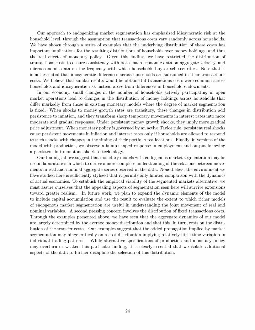
Our approach to endogenizing market segmentation has emphasized idiosyncratic risk at thehousehold level, through the assumption that transactions costs vary randomly across households.We have shown through a series of examples that the underlying distribution of these costs hasimportant implications for the resulting distributions of households over money holdings, and thusthe real e¤ects of monetary policy. Given this �nding, we have restricted the distribution oftransactions costs to ensure consistency with both macroeconomic data on aggregate velocity, andmicroeconomic data on the frequency with which households buy or sell securities. Note that itis not essential that idiosyncratic di¤erences across households are subsumed in their transactionscosts. We believe that similar results would be obtained if transactions costs were common acrosshouseholds and idiosyncratic risk instead arose from di¤erences in household endowments.

In our economy, small changes in the number of households actively participating in openmarket operations lead to changes in the distribution of money holdings across households thatdi¤er markedly from those in existing monetary models where the degree of market segmentationis �xed. When shocks to money growth rates are transitory, these changes in distribution addpersistence to in�ation, and they transform sharp temporary movements in interest rates into moremoderate and gradual responses. Under persistent money growth shocks, they imply more gradualprice adjustment. When monetary policy is governed by an active Taylor rule, persistent real shockscause persistent movements in in�ation and interest rates only if households are allowed to respondto such shocks with changes in the timing of their portfolio reallocations. Finally, in versions of themodel with production, we observe a hump-shaped response in employment and output followinga persistent but monotone shock to technology.

Our �ndings above suggest that monetary models with endogenous market segmentation may beuseful laboratories in which to derive a more complete understanding of the relations between move-ments in real and nominal aggregate series observed in the data. Nonetheless, the environment wehave studied here is su¢ ciently stylized that it permits only limited comparison with the dynamicsof actual economies. To establish the empirical viability of the segmented markets alternative, wemust assure ourselves that the appealing aspects of segmentation seen here will survive extensionstoward greater realism. In future work, we plan to expand the dynamic elements of the modelto include capital accumulation and use the result to evaluate the extent to which richer modelsof endogenous market segmentation are useful in understanding the joint movement of real andnominal variables. A second pressing concern involves the distribution of �xed transactions costs.Through the examples presented above, we have seen that the aggregate dynamics of our modelare largely determined by the average money distribution and that this, in turn, rests on the distri-bution of the transfer costs. Our examples suggest that the added propagation implied by marketsegmentation may hinge critically on a cost distribution implying relatively little time-variation inindividual trading patterns. While alternative speci�cations of production and monetary policymay overturn or weaken this particular �nding, it is clearly essential that we isolate additionalaspects of the data to further discipline the selection of this distribution.

24

References

[1] Alvarez, Fernando, Andrew Atkeson, and Chris Edmond (2003) �On the Sluggish Response ofPrices to Money in an Inventory-Theoretic Model of Money Demand�NBER Working Paperno. 10016.

[2] Alvarez, Fernando, Andrew Atkeson, and Patrick Kehoe (2002) �Money, Interest Rates andExchange Rates with Endogenously Segmented Markets�Journal of Political Economy 110(1),pages 73 - 112.

[3] Alvarez, Fernando, Robert E. Lucas, Jr., and Warren Weber (2001) �Interest Rates and In�a-tion�American Economic Review 91(2), pages 219 - 225.

[4] Chari, V.V., Patrick J. Kehoe and Ellen R. McGrattan (2000), �Sticky Price Models of theBusiness Cycle: Can the Contract Multiplier Solve the Persistence Problem?� Econometrica68(5), pages 1151-1179.

[5] Chatterjee, Satyajit and Dean Corbae (1992) �Endogenous Market Participation and the Gen-eral Equilibrium Value of Money�Journal of Political Economy 100(5), pages 615 - 646.

[6] Chiu, Jonathan (2005) �Endogenously Segmented Asset Market in an Inventory TheoreticModel of Money Demand�University of Western Ontario working paper.

[7] Christiano, Lawrence J., Martin Eichenbaum, and Charles L. Evans (1999) �Monetary PolicyShocks: What Have We Learned and to What End?� chapter 14 in Michael Woodford andJohn B. Taylor (eds.) Handbook of Macroeconomics IA. Elsevier Science.

[8] Dotsey, Michael, Robert G. King, and Alexander L. Wolman (1999) �State-Dependent Pricingand the General Equilibrium Dynamics of Money and Output�Quarterly Journal of Economics114, pages 655�690.

[9] Friedman, Milton (1968) �The Role of Monetary Policy�The American Economic Review 58(1),pages 1-17.

[10] Friedman, Milton (1980) Memorandum to U.K. Treasury and Civil Service Committee regard-ing �Enquiry Into Monetary Policy,�House of Commons, United Kingdom, 1980 July.

[11] Grossman, Sanford, and Laurence Weiss (1983) �A Transactions-Based Model of the MonetaryMechanism�American Economic Review 73(5), pages 871-880.

[12] King, Robert G. and Julia K. Thomas (2005) �Partial Adjustment without Apology�Interna-tional Economic Review (forthcoming).

[13] King, Robert G. and Mark W. Watson (1996) �Money, Prices, Interest Rates and the BusinessCycle�Review of Economics and Statistics pages 35 - 53

[14] Leeper, Eric M., Christopher A. Sims, and Tao Zha (1996) �What Does Monetary Policy Do?�Brookings Papers on Economic Activity 1996(2), pages 1 - 78.

[15] Rotemberg, Julio J. (1984) �A Monetary Equilibrium Model with Transactions Costs�92(1),pages 40-58.

25

[16] Thomas, Julia K. (2002) �Is Lumpy Investment Relevant for the Business Cycle?� Journal ofPolitical Economy, 110(3), pages 508�534.

[17] Uhlig, Harald (2004) �What Are the E¤ects of Monetary Policy on Output? Results from anAgnostic Identi�cation Procedure�Journal of Monetary Economics (forthcoming).

[18] Vissing-Jørgensen, Annette (2002) �Towards an Explanation of Household Portfolio ChoiceHeterogeneity: Non�nancial Income and Participation Cost Structures�NBER working paper8884.

[19] Williamson, Stephen D. (2005) �Monetary Policy and Distribution�University of Iowa workingpaper.

26

0 1 2 3 4 50

0.2

0.4

0.6

0.8

1

time-since-active

FIGURE 1A: Endogenous Segmentation Steady-State (mean duration: 4.818)

individual velocitiesassociated population fractions

0 1 2 3 40

0.2

0.4

0.6

0.8

1

time-since-active

FIGURE 1B: Fixed Duration Steady-State (mean duration: 5)

individual velocitiesassociated population fractions

1 2 3 4 5 6 7 8 9 10-0.5

0

0.5

1 FIGURE 2: A Temporary Money Growth Shock in the 5-Period Fixed Duration Model

perc

enta

ge p

oint

cha

nge

money growth rateinflation rate

1 2 3 4 5 6 7 8 9 10-3

-2

-1

0

1

perc

enta

ge p

oint

cha

nge

nominal interest ratereal interest rate

1 2 3 4 5 6 7 8 9 10-0.5

0

0.5

perc

ent d

evia

tion

date

aggregate real balancesaggregate velocity

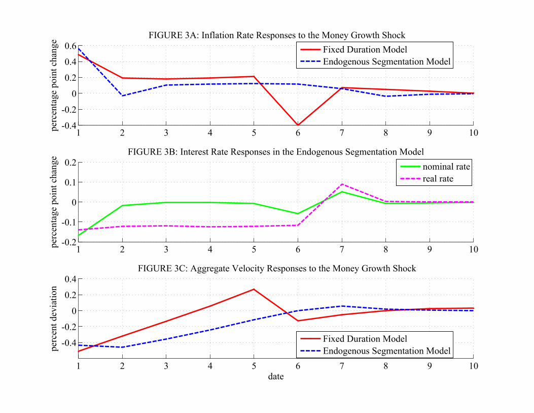
1 2 3 4 5 6 7 8 9 10-0.4

-0.2

0

0.2

0.4

0.6 FIGURE 3A: Inflation Rate Responses to the Money Growth Shock

perc

enta

ge p

oint

cha

nge

Fixed Duration ModelEndogenous Segmentation Model

1 2 3 4 5 6 7 8 9 10-0.2

-0.1

0

0.1

0.2 FIGURE 3B: Interest Rate Responses in the Endogenous Segmentation Model

perc

enta

ge p

oint

cha

nge

nominal ratereal rate

1 2 3 4 5 6 7 8 9 10

-0.4

-0.2

0

0.2

0.4 FIGURE 3C: Aggregate Velocity Responses to the Money Growth Shock

perc

ent d

evia

tion

date

Fixed Duration ModelEndogenous Segmentation Model

1 2 3 4 5 6 7 8 9 10-1

0

1

2

3

4

5FIGURE 4A: Endogenous Segmentation Response in Total Active Households

perc

ent d

evia

tion

1 2 3 4 5 6 7 8 9 10-0.1

0

0.1

0.2

0.3

0.4

FIGURE 4B: Endogenous Segmentation Response in Consumption of Active Households

perc

ent d

evia

tion

date

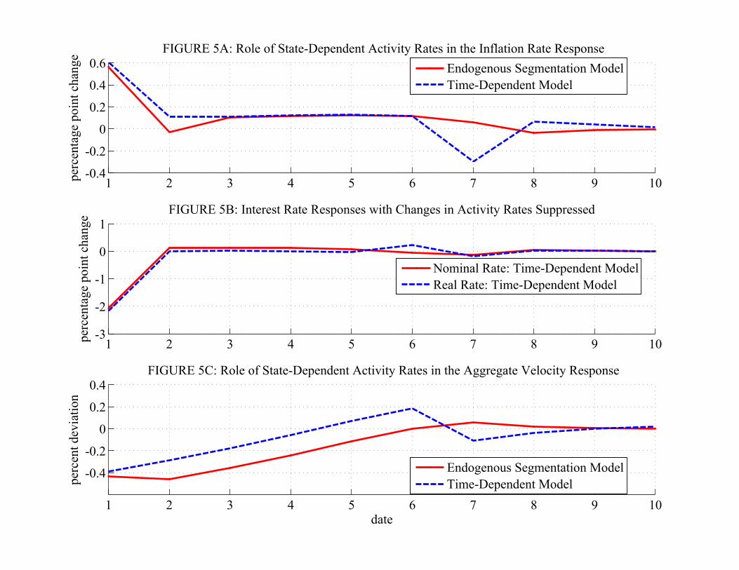
1 2 3 4 5 6 7 8 9 10-0.4

-0.2

0

0.2

0.4

0.6 FIGURE 5A: Role of State-Dependent Activity Rates in the Inflation Rate Response

perc

enta

ge p

oint

cha

nge

Endogenous Segmentation ModelTime-Dependent Model

1 2 3 4 5 6 7 8 9 10-3

-2

-1

0

1 FIGURE 5B: Interest Rate Responses with Changes in Activity Rates Suppressed

perc

enta

ge p

oint

cha

nge

Nominal Rate: Time-Dependent ModelReal Rate: Time-Dependent Model

1 2 3 4 5 6 7 8 9 10

-0.4

-0.2

0

0.2

0.4 FIGURE 5C: Role of State-Dependent Activity Rates in the Aggregate Velocity Response

perc

ent d

evia

tion

date

Endogenous Segmentation ModelTime-Dependent Model

1 2 3 4 5 6 7 8 9 10 11 12 13 14 15

-0.5

0

0.5

1

1.5 FIGURE 6: Temporary Money Growth Shock in a High Tranfer Costs Endogenous Segmentation Model

perc

enta

ge p

oint

cha

nge

money growth rateinflation rate

1 2 3 4 5 6 7 8 9 10 11 12 13 14 15

-0.4-0.2

00.20.40.6

perc

enta

ge p

oint

cha

nge

nominal interest ratereal interest rate

1 2 3 4 5 6 7 8 9 10 11 12 13 14 15

-0.5

0

0.5

real balances and velocity

perc

ent d

evia

tion

date

aggregate real balancesaggregate velocity

1 2 3 4 5 6 7 8 9 10 11 12 13 14 15

-0.5

0

0.5

1

1.5 FIGURE 7: Temporary Money Growth Shock in a High Mean Duration Endogenous Segmentation Model

perc

enta

ge p

oint

cha

nge

money growth rateinflation rate

1 2 3 4 5 6 7 8 9 10 11 12 13 14 15

-0.4-0.2

00.20.40.6

perc

enta

ge p

oint

cha

nge

nominal interest ratereal interest rate

1 2 3 4 5 6 7 8 9 10 11 12 13 14 15

-0.5

0

0.5

real balances and velocity

perc

ent d

evia

tion

date

aggregate real balancesaggregate velocity

1 2 3 4 5 6 7 8 9 10 11 12 13 14 150

0.005

0.01

0.015

0.02

0.025

0.03

date

dev

iatio

n fr

om in

itial

tren

d

Figure 8: Money and Prices with a Persistent Money Growth Shock

Money Stock Price Level Price Level in Fixed Duration model

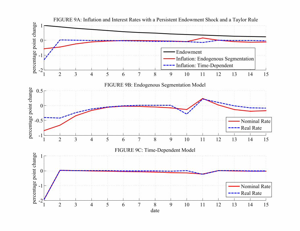
1 2 3 4 5 6 7 8 9 10 11 12 13 14 15-2

-1

0

1 FIGURE 9A: Inflation and Interest Rates with a Persistent Endowment Shock and a Taylor Rule

perc

enta

ge p

oint

cha

nge

EndowmentInflation: Endogenous SegmentationInflation: Time-Dependent

1 2 3 4 5 6 7 8 9 10 11 12 13 14 15-1

-0.5

0

0.5 FIGURE 9B: Endogenous Segmentation Model

perc

enta

ge p

oint

cha

nge

Nominal RateReal Rate

1 2 3 4 5 6 7 8 9 10 11 12 13 14 15-2

-1

0

1 FIGURE 9C: Time-Dependent Model

perc

enta

ge p

oint

cha

nge

date

Nominal RateReal Rate

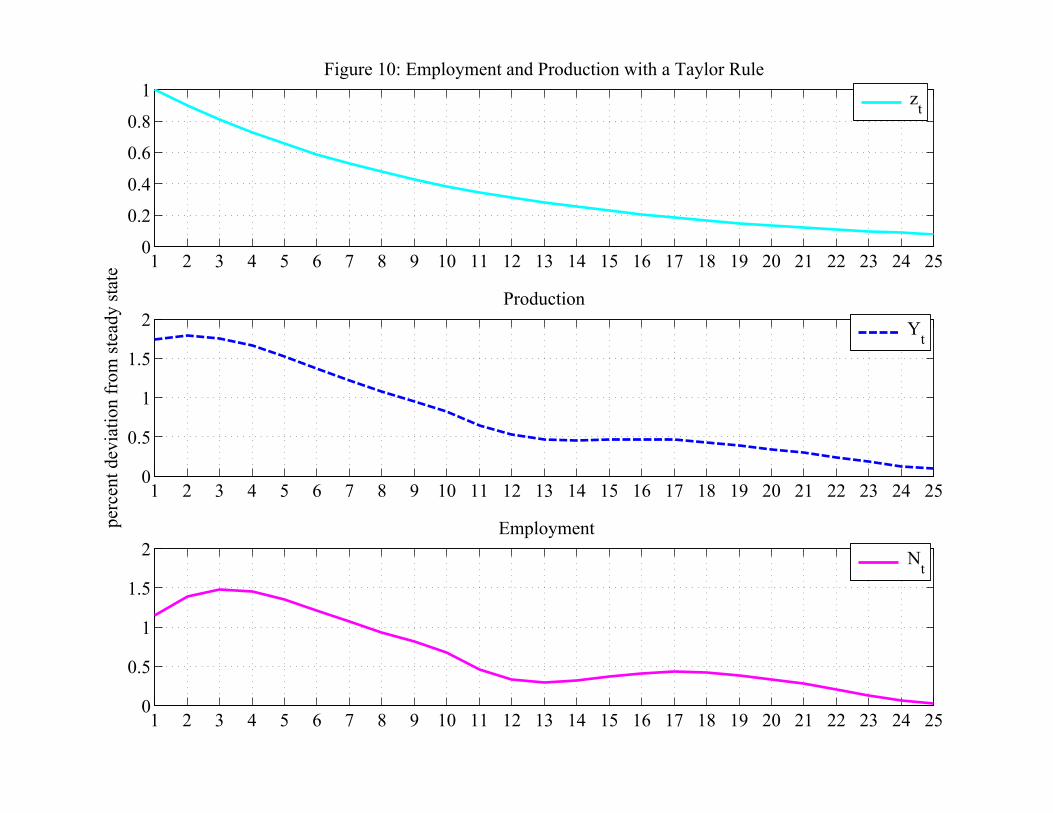
1 2 3 4 5 6 7 8 9 10 11 12 13 14 15 16 17 18 19 20 21 22 23 24 250

0.2

0.4

0.6

0.8

1 Figure 10: Employment and Production with a Taylor Rule

zt

1 2 3 4 5 6 7 8 9 10 11 12 13 14 15 16 17 18 19 20 21 22 23 24 250

0.5

1

1.5

2 Production

per

cent

dev

iatio

n fr

om st

eady

stat

e

Yt

1 2 3 4 5 6 7 8 9 10 11 12 13 14 15 16 17 18 19 20 21 22 23 24 250

0.5

1

1.5

2 Employment

Nt

Appendix

A Risk sharing

As described in the main text, bonds issued by a competitive �nancial intermediary are con-tingent on both aggregate and idiosyncratic shocks. The supply of these bonds is created usingpurchases of government bonds and free entry into intermediation implies a zero-pro�t condition.

Our �rst lemma derives the equilibrium price of households�bonds. Given the aggregate historyst, the intermediary�s pro�t when next period�s aggregate shock is st+1 solves the problem in (8)- (9). There, recall that households identi�ed by the history �t purchase B

�st; st+1; �

t; �t+1�units

of nominal bonds that pay one unit of currency next period if the aggregate shock is given by st+1and their idiosyncratic shock is �t+1, and the measure of such households is h

��t�.

Lemma 1 The equilibrium price of state-contingent bonds issued by the �nancial intermediary,q�st; st+1; �t+1

�; is given by q

�st; st+1; �t+1

�= q

�st; st+1

�h��t+1

�.

Proof. Substitution of the right-hand side of (9) for B�st; st+1

�in (8) givesZ

�t

Z�t+1

q�st; st+1; �t+1

�B�st; st+1; �

t; �t+1�h��t�d�t+1d�

t

�q�st; st+1

� Z�t

Z�t+1

B�st; st+1; �

t; �t+1�h��t�h��t+1

�d�t+1d�

t

=

Z�t

Z�t+1

�q�st; st+1; �t+1

�� q

�st; st+1

�h��t+1

��h��t�B�st; st+1; �

t; �t+1�d�t+1d�

t

= 0.

The last equality follows from the zero pro�t condition.

B Characterizing household behavior under risk-sharing

This section provides the main results we use in our numerical approach to solving the model.Lemma 2 proves that, given risk-sharing in the brokerage account, beginning of period moneybalances capture all relevant di¤erences across households at the start of any period. Additionalresults in lemma 3 establish that whenever households access their brokerage account, there isuniformity of actions in that they choose the same consumption and bank account balance regardlessof their past history of idiosyncratic shocks. The importance of this is that any di¤erences acrosshouseholds will be limited by the number of periods since active transactions between the bank andbrokerage account. Such di¤erences disappear whenever households with di¤erent bank accountbalances access their brokerage account at the same time. Finally, lemma 4 proves that households�follow a threshold rule in determining the timing of their account transfers; speci�cally, it showsthat households choose to become active whenever their current �xed transfer cost falls below somethreshold value that is common to all households with the same beginning-of-period bank balance.

We begin by deriving a lifetime budget constraint associated with the brokerage account. Usinglemma 1, the brokerage budget constraint for any household in the initial period is:

B �Zs1

Z�1

q (s1)h (�1)B (s1; �1) d�1ds1. (24)

i

In period 1, the brokerage account constraint is:

B (s1; �1) �Zs2

Z�2

q (s1; s2)h (�2)B (s1; s2; �1; �2) d�2ds2

� (1� �)P (s0) y (s0) +�x (s1; �1) + P (s1) �1

�z (s1; �1)

which, substituted into (24), gives:

B �Zs1

Z�1

q (s1)h (�1)hZs2

Z�2

q (s1; s2)h (�2)B (s1; s2; �1; �2) d�2ds2 � (1� �)P (s0) y (s0)

+�x (s1; �1) + P (s1) �1

�z (s1; �1)

id�1ds1

=

Zs2

Z�2q�s2�h��2�B (s1; s2; �1; �2) d�

2ds2 �Zs1

Z�1

q (s1)h (�1)h(1� �)P (s0) y (s0)

��x (s1; �1) + P (s1) �1

�z (s1; �1)

id�1ds1,

where we use the notation q�st�= q (s1) � q (s1; s2) � � � q

�st�1; st

�and h

��t�= h (�1) � � �h (�t).

Repeated substitutions for B�sj ; �j

�for j = 2; : : : ; t using (3) leads to the following equation.

B �Zst

Z�tq�st�h��t�B�st; �t

�d�tdst �

t�1Xj=1

Zsj

Z�jq�sj�h��j� h(1� �)P

�sj�1

�y�sj�1

���x�sj ; �j

�+ P

�sj��j

�z�sj ; �j

�id�jdsj .

Taking the limit of the above equation, given the No-Ponzi condition,

limt!1

Zst

Z�tq�st�h��t�B�st; �t

�dstd�t � 0;

we arrive at the following lifetime budget constraint associated with the brokerage account.

B �1Xt=1

Z Zq�st�h��t� �z(st; �t)

hx�st; �t

�+ P

�st��t

i� P

�st�1

�(1� �) y

�st�1

��d�tdst (25)

Equation 25, which is an immediate implication of the availability of a complete set of state-contingent bonds for each household, implies that individual histories are irrelevant beyond currentmoney balances in the bank account. This intuitive property of the model is straightforward, ifnotationally cumbersome, to prove and is important in our approach to characterizing competitiveequilibrium.

Lemma 2 Given M�st�1; �t�1

�, the decisions c

�st; �t

�, A

�st; �t

�, x�st; �t

�and z

�st; �t

�are in-

dependent of the history �t�1.

Proof. Equation 25 is equivalent to the following sequence of period by period constraints,

B�st�=

Zst+1

q�st; st+1

�B�st; st+1

�dst+1 � (1� �)P

�st�1

�y�st�1

�(26)

+

Z�th��t� hx�st; �t

�+ P

�st��t

iz�st; �t

�d�t,

ii

and the limit condition

limt!1

Zstq�st�B�st�dst = 0: (27)

Let �t+jt =��t; : : : ; �t+j

be a partial history of individual household shocks , �x

�st; �t

�and de�ne

pointwise the continuation value to the household�s problem given�B�st�;M

�st�1; �t�1

��as

V�B0;M0; s

t; �t�= max

1Xj=0

�jZst+jt

Z�t+jt

u�chst+j ; �t+jt

i�g�st+j j st

�h��t+jt

�dst+jt d�t+jt

subject to:

B�st+j

�=

Zst+j+1

q�st+j ; st+j+1

�B�st+j ; st+j+1

�dst+j+1 � (1� �)P

�st+j�1

�y�st+j�1

�+

Z�t+jt

h��t+jt

� hx�st+j ; �t+jt

�+ P

�st+j

��t+j

iz�st+j ; �t+jt

�d�t+jt ; for j = 0; : : : ;

P�st+j

�c�st+j ; �t+jt

��M

�st+j�1; �t+j�1t�1

�+ x

�st+j ; �t+jt

�z�st+j ; �t+jt

��A

�st+j ; �t+jt

�, for j = 0; : : : ,

M�st+j ; �t+jt

�� A

�st+j ; �t+jt

�+ �P

�st+j

�y�st+j

�and A

�st+j ; �t+jt

�� 0, for j = 0; : : : ,

given B�st�= B0; M

�st�1; �t�1t�1

�=M0 and lim

j!1

Zst+jt

q�st+j

�B�st+j

�dst+jt = 0.

Clearly the optimal choices of c�st+k; �t+kt

�; A

�st+k; �t+kt

�, x�st+k; �t+kt

�and z

�st+k; �t+kt

�, for

any k = 0; 1; : : :, are independent of �t�1given M0. Let c�st+k; �t+kt ;M0

�; A

�st+k; �t+kt ;M0

�,

x�st+k; �t+kt ;M0

�and z

�st+k; �t+kt ;M0

�describe these choices. Next, any solution to the house-

hold�s problem must also solve the following problem.

maxt�1Xj=1

�j�1Zsj

Z�ju�c�sj ; �j

��g�sj�h��j�dsjd�j

+�tZst

Z�tV�B�st�;M

�st�1; �t�1

�; st; �t

�g�st�h��t�dstd�t

subject to

B�sj�=

Zsj+1

q�sj ; sj+1

�B�sj ; sj+1

�dsj+1 � (1� �)P

�sj�1

�y�sj�1

�+

Z�jh��j� hx�sj ; �j

�+ P

�sj��j

iz�sj ; �j

�d�j ,

P�sj�c�sj ; �j

��M

�sj�1; �j�1

�+ x

�sj ; �j

�z�sj ; �j

��A

�sj ; �j

�,

M�sj ; �j

�� A

�sj ; �j

�+ �P

�sj�y�sj�and A

�sj ; �j

�� 0, for j = 1; : : : ; t� 1.

In this problem, the optimal choices of c�st+k; �t+k

�, A�st+k; �t+k

�, x�st+k; �t+k

�and z

�st+k; �t+k

�,

for any k = 0; 1; : : :, are given by the functions c�st+k; �t+kt ;M

�st�1; �t�1

��,

iii

A�st+k; �t+kt ;M

�st�1; �t�1

��, x�st+k; �t+kt ;M

�st�1; �t�1

��and z

�st+k; �t+kt ;M

�st�1; �t�1

��,

which attained the maximum value V�B�st�;M

�st�1; �t�1

�; st; �t

�.

We proceed to further characterize household behavior by studying the state-contingent planschosen by households in period 0 when they are all identical. Let � denote the multiplier associatedwith equation 25 and �0

�st; �t

�be the LaGrange multiplier for (4) and �1

�st; �t

�the multiplier for

(5). For clarity, the Lagrangian is shown below.

L =1Xt=1

�t�1Zst

Z�t

�u�c�st; �t

��g�st�h��t�

+�0�st; �t

�g�st�h��t� hM�st�1; �t�1

�+ x

�st; �t

�z�st; �t

��A

�st; �t

�� P

�st�c�st; �t

�i+�1

�st; �t

�g�st�h��t� hA�st; �t

�+ �P

�st�y�st��M

�st; �t

�i�d�tdst

+�

�B +

1Xt=1

Zstq�st� h(1� �)P

�st�1

�y�st�1

�dst

�1Xt=1

Zst

Z�tq�st�h��t� �x�st; �t

�+ P

�st��t

�z�st; �t

�d�tdst

�Given any choice of z

�st; �t

�, the household�s choices of c

�st; �t

�, A

�st; �t

�;M

�st; �t

�and

x�st; �t

�, satisfy the following conditions.

Du�c�st; �t

��� P

�st��0�st; �t

�= 0 (28)

��0�st; �t

�+ �1

�st; �t

�� 0, (29)

= 0 if A�st; �t

�> 0,

��1�st; �t

�+ �

Zst+1

Z�t+1

�0�st; st+1; �

t; �t+1�h��t+1

�g�st+1 j st

�dst+1d�t+1 � 0 (30)

= 0 if M�st; �t

�> �P

�st�y�st�

�t�1�0�st; �t

�g�st�h��t�� �q

�st�h��t�= 0 if z

�st; �t

�= 1. (31)

The following lemma shows that households choose the same consumption and subsequentmoney balances for their bank account whenever they pay transfer costs to access their brokerageaccounts. Recall that this result is important for the approach we take to characterizing householdbehavior in that it implies that heterogeneity across households is limited to periods when they areinactive.

Lemma 3 For any�st; �t

�in which z

�st; �t

�= 1, c

�st; �t

�, A

�st; �t

�and M

�st; �t

�are indepen-

dent of �t:

Proof. Given z�st; �t

�= 1, (28) and (31) imply

Du�c�st; �t

��=�q�st�P�st�

�t�1g (st). (32)

iv

As � is the same for all households, this proves that c�st; �t

�is independent of �t. Next, it is

su¢ cient to examine the case where A�st; �t

�> 0 and therefore M

�st; �t

�> �P

�st�y�st�. In this

case, (29) and (30) together give

�0�st; �t

�= �

Zst+1

Z�t+1

�0�st; st+1; �

t; �t+1�h��t+1

�g�st+1 j st

�dst+1d�t+1,

which, using (28) and (32) leads to the expression,

Du�c�st; �t

��= �

Zst+1

Z�t+1

Du�c�st+1; �t+1

�� "P �st+1�P (st)

#�1h��t+1

�g�st+1 j st

�dst+1d�t+1.

Since this expression must hold for all �t, it follows that c�st+1; �t+1

�is not a function of �t which,

given (4) and (5), implies that A�st; �t

�and thus M

�st; �t

�must be independent of �t.

Our �nal result shows that households follow threshold cost policies with respect to the costsof accessing their brokerage accounts

Lemma 4 For any�st; �t�1

�, A =

��t j z

�st; �t

�= 1

is a convex set bounded below by 0.

Proof. Assume not, let eA =��t j z

�st; �t

�= 1

and m eA =

R eA h (�) d�. De�ne � implicitly

using the equationR �0 h (�) d� = m eA. By the Axiom of Choice there exists a 1 � 1 function

S : eA !�0; ��. Given B

�st�and M

�st�1; �t�1

�, for each �0 2 eA and � = S (�0), construct an

alternate continuation plan that assigns the original continuation plan associated with �0 to �.In other words, ca

�st; �t�1; �

�= c

�st; �t�1; �0

�, Aa

�st; �t�1; �

�= A

�st; �t�1; �0

�and so on. This

alternative plan satis�es (3) - (6) and is thus feasible. Moreover, by construction, it o¤ers the sameexpected lifetime utility as the original plan. Any solution to the household�s problem, solving (2)subject to (3) - (6), must satisfy (25) with equality. Since the original plan solved the household�sproblem by assumption, the alternative plan satis�es (25) as a strict inequality sinceZ

�t�1q�st�h��t�1

� Z �

0

�xa�st; �t

�+ P

�st��t

�d�d�t�1

<

Z�tq�st�h��t� �x�st; �t

�+ P

�st��t

�z�st; �t

�d�tdst:

This contradicts optimality of the original plan.

v