Including all the lines1

Robert L. Kurucz

Abstract: I present a progress report on including all the lines in the line lists, including all the lines in the opacities, andincluding all the lines in the model atmosphere and spectrum synthesis calculations. The increased opacity will improve stel-lar atmosphere, pulsation, stellar interior, asteroseismology, nova, supernova, and other radiation-hydrodynamics calcula-tions. I also report on producing high-resolution, high-signal-to-noise atlases for use in verifying the line data and spectrumcalculations, and as tools for extending laboratory spectrum analyses to higher energy levels. All the data are available onmy web site: kurucz.harvard.edu.

PACS Nos: 31.15.ag, 31.30.Gs, 32.30.–r, 32.70.–n, 32.70.Cs, 33.20.–t, 33.70.Ca, 95.30.Ky, 95.75.Fg, 96.60.Fe, 96.60.Ub,97.10.Ex, 97.10.Tk, 97.60.Bw

Résumé : Je présente un rapport des progrès faits pour inclure toutes les raies dans les listes de raies, incluant toutes lesraies dans les opacités et incluant toutes les raies dans les calculs de modèle d’atmosphère et de synthèse de spectre. L’opa-cité accrue va améliorer les calculs d’atmosphère stellaire, de pulsation, d’intérieur stellaire, d’astérosismologie, de nova etde supernova, ainsi que ceux touchant les autres phénomènes de radiation-hydrodynamique. Je présente aussi un rapport surla production d’atlas de haute résolution et de haut rapport signal sur bruit à être utilisés dans la vérification des données deraies et les calculs de spectres et comme outils pour étendre les analyses des spectres pris en laboratoire vers des niveauxplus hauts. Toutes les données sont disponibles sur mon site web : kurucz.harvard.edu.

[Traduit par la Rédaction]

1. IntroductionIn 1965, I started collecting and computing atomic and

molecular line data for computing opacities in model atmos-pheres and then for synthesizing spectra. I wanted to deter-mine stellar effective temperatures, gravities, and abundances.I still want to.For 23 years I included more and more lines, but I could

never get a solar model to look right, to reproduce the ob-served energy distribution.In 1988, I finally produced enough lines, I thought. I com-

pleted a calculation of the first 9 ions of the iron group ele-ments, shown in Table 1, using my versions of Cowan'satomic structure programs [1] and the compilation of labora-tory energy levels by Sugar and Corliss [2]. There were datafor 42 million lines that I combined with data for 1 millionlines from my earlier list for lighter and heavier elements, in-cluding all the data from the literature. In addition, I hadcomputed line lists for diatomic molecules including 15 mil-lion lines of H2, CH, NH, OH, MgH, SiH, C2, CN, CO, SiO,and TiO for a total of 58 million lines.I then tabulated 2 nm resolution opacity distribution func-

tions (ODFs) from the line list for temperatures from 2 000 to200 000 K and for a range of pressure suitable for stellar at-mospheres [3].Using the ODFs I computed a theoretical solar model [4]

with the solar effective temperature and gravity, the current

solar abundances from [5], mixing-length to scale-height ratiol/H = 1.25, and constant microturbulent velocity 1.5 km s–1. Itgenerally matched the observed energy distribution from [6].I computed thousands of model atmospheres that I distrib-

uted on magnetic tapes, then on CDs, and now on my website, kurucz.harvard.edu. They made observers happy. How-ever, agreement with low-resolution observations of inte-grated properties does not imply correctness.

2. ProblemsIn 1988 the abundances were wrong, the microturbulent

velocity was wrong, the convection was wrong, and the opac-ities were wrong.Since 1965 the Fe abundance has varied by over a factor

of 10. In 1988 the Fe abundance was 1.66 times larger thantoday. There was mixing-length convection with an exagger-ated, constant microturbulent velocity. In the grids of models,the default microturbulent velocity was 2 km s–1. My 1Dmodels still have mixing-length convection, but now with adepth-dependent microturbulent velocity that scales with theconvective velocity. 3D models with cellular convection donot have microturbulent velocity at all but use the dopplershifts from the convective motions.In 1988 the line opacity was underestimated, because not

enough lines were included in the line lists. Table 2 is anoutline for the Fe II line calculation at that time. The higher

Received 28 September 2010. Accepted 9 November 2010. Published at www.nrcresearchpress.com/cjp on 6 May 2011.

R.L. Kurucz. Harvard-Smithsonian Center for Astrophysics, Cambridge, MA 02138, USA.

E-mail for correspondence: rkurucz@cfa.harvard.edu1This article is part of a Special Issue on the 10th International Colloquium on Atomic Spectra and Oscillator Strengths for Astrophysicaland Laboratory Plasmas.

417

Can. J. Phys. 89: 417–428 (2011) doi:10.1139/P10-104 Published by NRC Research Press

Can

. J. P

hys.

Dow

nloa

ded

from

ww

w.n

rcre

sear

chpr

ess.

com

by

LA

FAY

ET

TE

CO

LL

EG

E o

n 04

/18/

14Fo

r pe

rson

al u

se o

nly.

energy levels that produce series of lines that merge into ul-traviolet (UV) continua were not included. Those levels alsoproduce huge numbers of weaker lines in the visible and in-frared (IR) that blend and fill in the spaces between thestronger lines. Also, lines of heavier elements were not sys-tematically included. Moreover, the additional broadeningfrom hyperfine and isotopic splitting was not included.In 1988 the opacities were low but were balanced by high

abundances that made the lines stronger and by high microtur-bulent velocity that made the lines broader. Now, the abundan-ces, the convection, and the opacities are still wrong, but theyhave improved. I am concentrating on filling out the line lists.

3. Examples of new calculations

In Tables 3 to 5 I show sample statistics from my newsemi-empirical calculations for Fe II, Ni I, and Co I to illus-trate how important it is to do the basic physics well and howmuch data there are to deal with. Ni, Co, and Fe are promi-nent in supernovae, including both radioactive and stable iso-topes. There is not space here for the lifetime and gfcomparisons. Generally, low configurations that have beenwell studied in the laboratory produce good lifetimes and gfvalues, while higher configurations that are poorly observed

and are strongly mixed are not well constrained in least-squares fits and necessarily produce poorer results and largescatter. My hope is that the predicted energy levels can helpthe laboratory spectroscopists to identify more levels and fur-ther constrain the least-squares fits. From my side, I checkthe computed gf values in spectrum calculations by compar-ing with observed spectra. I adjust the gf values so that thespectra match. Then I search for patterns in the adjustmentsthat suggest corrections in the least-squares fits.As the new calculations accumulate I put on my web site

the output files of the least-squares fits to the energy levels,energy level tables, with E and J, identification, strongest ei-genvector components, lifetime, A-sum, C4, C6, Landé g. Thesums are complete up to the first (n= 10) energy level notincluded. There are electric dipole (E1), magnetic dipole(M1), and electric quadrupole (E2) line lists. Radiative, Stark,and van der Waals damping constants and Landé g values areautomatically produced for each line. Branching fractions arealso computed. Hyperfine and isotopic splitting are includedwhen the data exist, but not automatically. Eigenvalues are re-placed by measured energies, so that lines connecting meas-ured levels have correct wavelengths. Most of the lines haveuncertain wavelengths, because they connect predicted ratherthan measured levels. Laboratory measurements of gf valuesand lifetimes will be included. Measured or estimated widthsof auto-ionizing levels will be included when available. Thepartition function is tabulated for a range of densities.When computations with the necessary information are

available from other workers, I am happy to use those datainstead of repeating the work.Once the line list for an ion or molecule is validated it will

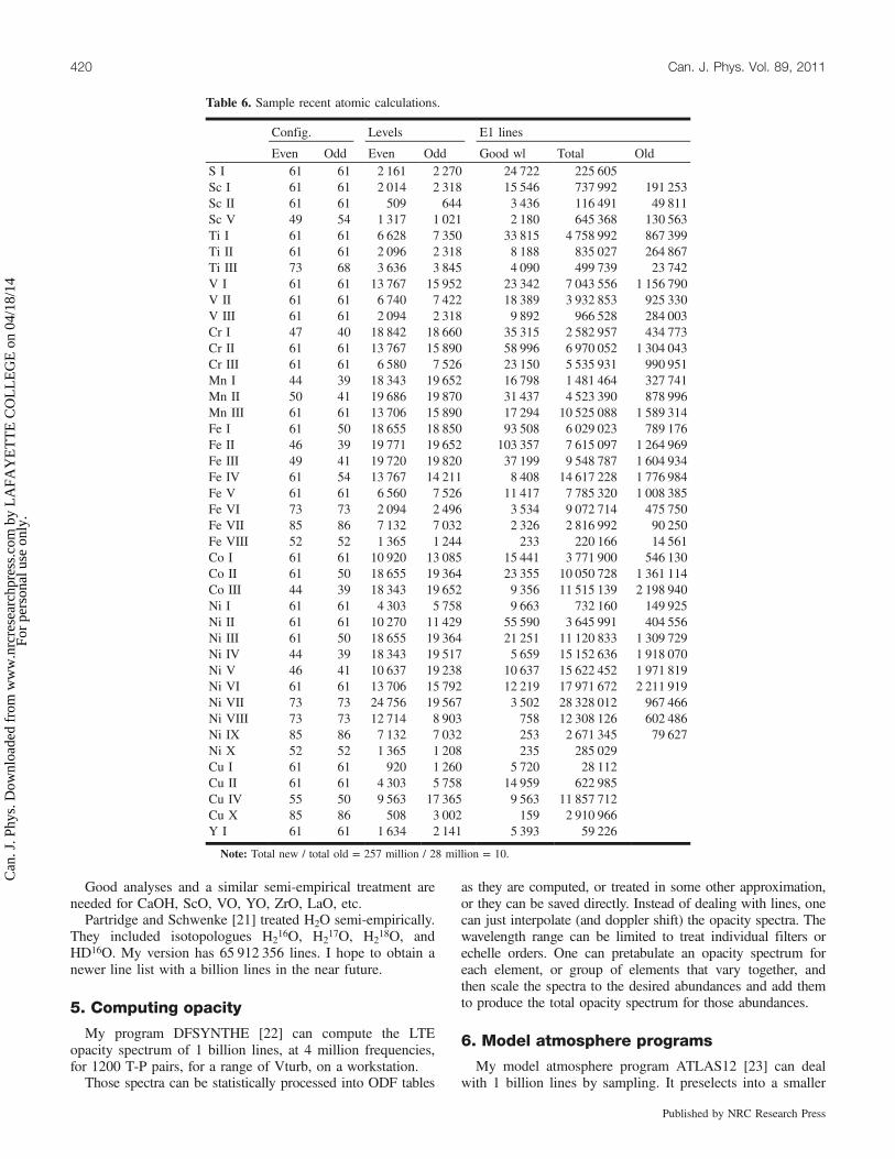
be incorporated into the wavelength sorted line lists on myweb site for computing opacities or detailed spectra. Theweb directories are located at kurucz.harvard.edu/atoms.htmland kurucz.harvard.edu/molecules.html for the details, andkurucz.harvard.edu/linelists.html for the completed line lists.Table 6 presents line statistics from some of my recent cal-

culations that show an order of magnitude increase over myearlier work, because I am treating about 3 times as manylevels. Considering only the ions in the table, there are about257 million lines compared to 26 million in the 1988 calcu-lation. Table 7 shows my estimate (individual ions only to as-tronomical accuracy) that my line lists will have severalbillion atomic and molecular lines if I can continue mywork. I expect to update and replace all my previous calcula-tions for lighter elements and for the iron group in the nearfuture. Then I will concentrate on extending the work toheavier elements and higher ions.

Table 1. Iron group lines computed at San Diego supercomputer center 1988.

I II III IV V VI VII VIII IXCa 48 573 4 227 11 740 113 121 330 004 217 929 125 560 30 156 22 803Sc 191 253 49 811 1 578 16 985 130 563 456 400 227 121 136 916 30 587Ti 867 399 264 867 23 742 5 079 37 610 155 919 356 808 230 705 139 356V 1 156 790 925 330 284 003 61 630 8 427 39 525 160 652 443 343 231 753Cr 434 773 1 304 043 990 951 366 851 73 222 10 886 39 668 164 228 454 312Mn 327 741 878 996 1 589 314 1 033 926 450 293 79 068 14 024 39 770 147 442Fe 789 176 1 264 969 1 604 934 1 776 984 1 008 385 475 750 90 250 14 561 39 346Co 546 130 1 048 188 2 198 940 1 569 347 2 032 402 1 089 039 562 192 88 976 15 185Ni 149 926 404 556 1 309 729 1 918 070 1 971 819 2 211 919 967 466 602 486 79 627

Table 2. Fe II in 1988 based on [7] and on [2].

Even: 22 configurations; 5723 levels; 354 known levels; 729 Hamilto-nian parameters, all CI; 46 free LS parameters; standard deviation142 cm–1

d7

d64s d54s2 d64d d54s4d d44s24d d54p2

d65s d54s5s d65d d54s5d d65gd66s d54s6s d66d d54s6d d66gd67s d67d d67gd68s d68dd69s

Odd: 16 configurations; 5198 levels; 435 known levels; 541 Hamil-tonian parameters, all CI; 43 free LS parameters; standard deviation135 cm–1

d64p d54s4p d64f d54s4f d44s24p

d65p d54s5p d65fd66p d54s6p d66fd67p d54s7pd68p d54s8pd69pTotal E1 lines saved 1 254 969E1 lines with good wavelengths 45 815

418 Can. J. Phys. Vol. 89, 2011

Published by NRC Research Press

Can

. J. P

hys.

Dow

nloa

ded

from

ww

w.n

rcre

sear

chpr

ess.

com

by

LA

FAY

ET

TE

CO

LL

EG

E o

n 04

/18/

14Fo

r pe

rson

al u

se o

nly.

4. TiO and H2O

These are examples of incorporating data from other re-searchers.Schwenke [19] calculated energy levels for TiO, including

in the Hamiltonian the 20 lowest vibration states of the 13lowest electronic states of TiO (singlets a, b, c, d, f, g, h and

triplets X, A, B, C, D, E) and their interactions. He deter-mined parameters by fitting the observed energies or by com-puting theoretical values. Using Langhoff's [20] transitionmoments, Schwenke generated a line list for J= 0 to 300 forthe isotopologues 46Ti16O, 47Ti16O. 48Ti16O, 49Ti16O, and50Ti16O with fractional abundances 0.080, 0.073, 0.738,0.055, and 0.054 . My version has 37 744 499 lines.

Table 3. Fe II based on [2, 7–14].

Even: 46 configurations; 19771 levels; 421 known levels; 2645 Hamiltonian parameters, all CI; 48 free LS parameters; stan-dard deviation 48 cm–1

d7

d64s d54s2 d64d d54s4d d44s24d d54p2

d65s d54s5s d65d d54s5d d65g d54s5g d44s25sd66s d54s6s d66d d54s6d d66g d54s6gd67s d54s7s d67d d54s7d d67g d54s7g d67i d54s7id68s d54s8s d68d d54s8d d68g d54s8g d68i d54s8i d54s9ld69s d54s9s d69d d54s9d d69g d54s9g d69i d54s9i d69lOdd: 39 configurations; 19652 levels; 596 known levels; 2996 Hamiltonian parameters, all CI; 48 free LS parameters; stan-dard deviation 64 cm–1

d64p d54s4p d64f d54s4f d44s24p d44-s24f

d65p d54s5p d65f d54s5f d44s25pd66p d54s6p d66f d54s6f d66h d54s6hd67p d54s7p d67f d54s7f d67h d54s7hd68p d54s8p d68f d54s8f d68h d54s8h d68k d54s8kd69p d54s9p d69f d54s9f d69h d54s9h d69k d54s9kTotal E1 lines saved 7 615 097 new 1 254 969 old ratio = 6.1E1 lines with good wavelengths 103 357 new 45 815 old ratio = 2.3Forbidden lines M1 even M1 odd E2 even E2 oddTotal lines saved 2 707 590 3 665 949 10 861 275 13 550 604With good wavelengths 38 256 66 961 59 008 110 668Between metastable 1232 0 1827 0Isotope 54Fe 55Fe 56Fe 57Fe 58Fe 59Fe 60FeFraction 0.059 0.0 0.9172 0.021 0.0028 0.0 0.0

Note: 57Fe has not yet been measured, because it has hyperfine splitting. Rosberg et al. [15] have measured 56Fe–54Fe in 9 lines and 58Fe–56Fein one line. I split the computed lines by hand. The data from these papers after Sugar and Corliss [2] are not in the NIST atomic energy leveldatabase.

Table 4. Ni I based on Litzén et al. [16] with isotopic splitting.

Total E1 lines saved 732 160 new 149 926 old ratio = 4.9

E1 lines with good wavelengths 9663 new 3949 old ratio = 2.4Isotope 56Ni 57Ni 58Ni 59Ni 60Ni 61Ni 62Ni 63Ni 64NiFraction 0.0 0.0 0.6827 0.0 0.2790 0.0113 0.0359 0.0 0.0091

Note: There are measured isotopic splittings for 326 lines from which I determined 131 energy levels relative to the ground. Theselevels are connected by 11670 isotopic lines. Hyperfine splitting was included for 61Ni, but only 6 levels have been measured, whichproduce 4 lines with 38 components. A pure isotope laboratory analysis is needed. Ni I lines are asymmetric from the splitting andthey now agree in shape with lines in the solar spectrum.

Table 5. Co I based on Pickering and Thorne [17] and on Pickering [18] with hy-perfine splitting.

Total E1 lines saved 3 771 908 new 546 130 old ratio = 6.9

E1 lines with good wavelengths 15 441 new 9 879 old ratio = 2.4Isotope 56Co 57Co 58Co 59Co 60CoFraction 0.0 1. 0.0 0.0 0.0

Note: Hyperfine constants have been measured in 297 levels, which produce 244264 com-ponent E1 lines. The new calculation greatly improves the appearance of the Co I lines in thesolar spectrum.

Kurucz 419

Published by NRC Research Press

Can

. J. P

hys.

Dow

nloa

ded

from

ww

w.n

rcre

sear

chpr

ess.

com

by

LA

FAY

ET

TE

CO

LL

EG

E o

n 04

/18/

14Fo

r pe

rson

al u

se o

nly.

Good analyses and a similar semi-empirical treatment areneeded for CaOH, ScO, VO, YO, ZrO, LaO, etc.Partridge and Schwenke [21] treated H2O semi-empirically.

They included isotopologues H216O, H2

17O, H218O, and

HD16O. My version has 65 912 356 lines. I hope to obtain anewer line list with a billion lines in the near future.

5. Computing opacity

My program DFSYNTHE [22] can compute the LTEopacity spectrum of 1 billion lines, at 4 million frequencies,for 1200 T-P pairs, for a range of Vturb, on a workstation.Those spectra can be statistically processed into ODF tables

as they are computed, or treated in some other approximation,or they can be saved directly. Instead of dealing with lines, onecan just interpolate (and doppler shift) the opacity spectra. Thewavelength range can be limited to treat individual filters orechelle orders. One can pretabulate an opacity spectrum foreach element, or group of elements that vary together, andthen scale the spectra to the desired abundances and add themto produce the total opacity spectrum for those abundances.

6. Model atmosphere programs

My model atmosphere program ATLAS12 [23] can dealwith 1 billion lines by sampling. It preselects into a smaller

Table 6. Sample recent atomic calculations.

Config. Levels E1 lines

Even Odd Even Odd Good wl Total OldS I 61 61 2 161 2 270 24 722 225 605Sc I 61 61 2 014 2 318 15 546 737 992 191 253Sc II 61 61 509 644 3 436 116 491 49 811Sc V 49 54 1 317 1 021 2 180 645 368 130 563Ti I 61 61 6 628 7 350 33 815 4 758 992 867 399Ti II 61 61 2 096 2 318 8 188 835 027 264 867Ti III 73 68 3 636 3 845 4 090 499 739 23 742V I 61 61 13 767 15 952 23 342 7 043 556 1 156 790V II 61 61 6 740 7 422 18 389 3 932 853 925 330V III 61 61 2 094 2 318 9 892 966 528 284 003Cr I 47 40 18 842 18 660 35 315 2 582 957 434 773Cr II 61 61 13 767 15 890 58 996 6 970 052 1 304 043Cr III 61 61 6 580 7 526 23 150 5 535 931 990 951Mn I 44 39 18 343 19 652 16 798 1 481 464 327 741Mn II 50 41 19 686 19 870 31 437 4 523 390 878 996Mn III 61 61 13 706 15 890 17 294 10 525 088 1 589 314Fe I 61 50 18 655 18 850 93 508 6 029 023 789 176Fe II 46 39 19 771 19 652 103 357 7 615 097 1 264 969Fe III 49 41 19 720 19 820 37 199 9 548 787 1 604 934Fe IV 61 54 13 767 14 211 8 408 14 617 228 1 776 984Fe V 61 61 6 560 7 526 11 417 7 785 320 1 008 385Fe VI 73 73 2 094 2 496 3 534 9 072 714 475 750Fe VII 85 86 7 132 7 032 2 326 2 816 992 90 250Fe VIII 52 52 1 365 1 244 233 220 166 14 561Co I 61 61 10 920 13 085 15 441 3 771 900 546 130Co II 61 50 18 655 19 364 23 355 10 050 728 1 361 114Co III 44 39 18 343 19 652 9 356 11 515 139 2 198 940Ni I 61 61 4 303 5 758 9 663 732 160 149 925Ni II 61 61 10 270 11 429 55 590 3 645 991 404 556Ni III 61 50 18 655 19 364 21 251 11 120 833 1 309 729Ni IV 44 39 18 343 19 517 5 659 15 152 636 1 918 070Ni V 46 41 10 637 19 238 10 637 15 622 452 1 971 819Ni VI 61 61 13 706 15 792 12 219 17 971 672 2 211 919Ni VII 73 73 24 756 19 567 3 502 28 328 012 967 466Ni VIII 73 73 12 714 8 903 758 12 308 126 602 486Ni IX 85 86 7 132 7 032 253 2 671 345 79 627Ni X 52 52 1 365 1 208 235 285 029Cu I 61 61 920 1 260 5 720 28 112Cu II 61 61 4 303 5 758 14 959 622 985Cu IV 55 50 9 563 17 365 9 563 11 857 712Cu X 85 86 508 3 002 159 2 910 966Y I 61 61 1 634 2 141 5 393 59 226

Note: Total new / total old = 257 million / 28 million = 10.

420 Can. J. Phys. Vol. 89, 2011

Published by NRC Research Press

Can

. J. P

hys.

Dow

nloa

ded

from

ww

w.n

rcre

sear

chpr

ess.

com

by

LA

FAY

ET

TE

CO

LL

EG

E o

n 04

/18/

14Fo

r pe

rson

al u

se o

nly.

line list the lines that are relevant for the model. It defaults to30 000 sampling points, but it could sample a million. It cantreat arbitrary depth-dependent abundances and velocities.My program ATLAS9 [24] uses ODFs, so it is independ-

ent of the number of lines.

7. Atlases and spectrum synthesis

High-resolution, high signal-to-noise spectra are needed totest the line data and the spectrum synthesis programs and todetermine the stellar parameters.There are no high-quality solar spectra taken above the at-

mosphere in the UV, visible, or IR out to 2.2 mm. There is arecent central intensity atlas produced with an FTS on theACE satellite [25] that covers from 2.2 to 14 mm. I will fit theintensity spectrum by adjusting the line parameters, and then Iwill compute the irradiance spectrum with those line data.In the UV, there are not even “good” quality solar spectra.

There are various good quality solar spectra taken through

the atmosphere in the visible and IR. I have been trying toreduce the FTS spectra taken by James Brault from KittPeak to produce central intensity, limb intensity, flux, and ir-radiance atlases.Figure 1 shows the Kitt Peak flux atlas [26] for 300 to

1000 nm with resolving power greater than 300 000 and sig-nal-to-noise greater than 3000. Figure 2 is the telluric absorp-tion in the flux atlas. Most of the line data come from theHITRAN database [27]. Figure 3 is the Kitt Peak irradianceatlas [28] derived from the flux spectrum by removing thetelluric lines. Figure 4 shows a section of a similarly con-structed irradiance atlas [29] in the H band from 1580 to1740 and in the K band from 1920 to 2100 nm that I willextend.Line data can be tested by comparing calculated spectra to

the atlases. Figure 5 shows a sample spectrum calculationwith the lines labelled for a nearly empty angstrom of the so-lar flux atlas shown in Fig. 1. It shows the quality of the ob-served FTS spectrum from Kitt Peak, the computed telluric

Table 7. Estimated lines in 3d and 4d group sequences (in millions).

I II III IV V VI VII VIII IX X …Ca 0.05Sc 0.7 0.05Ti 5 0.7 0.05V 14 5 0.7 0.05Cr 10 14 5 0.7 0.05Mn 1.5 10 14 5 0.7 0.05Fe 6 7 10 14 5 0.7 0.05Co 4 10 7 10 14 5 0.7 0.05Ni 0.7 4 10 7 10 14 5 0.7 0.05Cu 0.03 0.6 4 10 7 10 14 5 0.7 0.05Zn 0.1 0.03 0.6 4 10 7 10 14 5 0.7 …Ga 0.1 0.03 0.6 4 10 7 10 14 5 …Ge 0.1 0.03 0.6 4 10 7 10 14 …As 0.1 0.03 0.6 4 10 7 10 …Se 0.1 0.03 0.6 4 10 7 …Br 0.1 0.03 0.6 4 10 …Kr 0.1 0.03 0.6 4 …Rb 0.1 0.03 0.6 …Sr 0.05 0.1 0.03 …Y 0.7 0.05 0.1 …Zr 5 0.7 0.05Nb 14 5 0.7 0.05Mo 10 14 5 0.7 0.05Tc 1.5 10 14 5 0.7 0.05Ru 6 7 10 14 5 0.7 0.05Rh 4 10 7 10 14 5 0.7 0.05Pd 0.7 4 10 7 10 14 5 0.7 0.05Ag 0.03 0.6 4 10 7 10 14 5 0.7 0.05Cd 0.1 0.03 0.6 4 10 7 10 14 5 0.7 …In 0.1 0.03 0.6 4 10 7 10 14 5 …Sn 0.1 0.03 0.6 4 10 7 10 14 …Sb 0.1 0.03 0.6 4 10 7 10 …Te 0.1 0.03 0.6 4 10 7 …I 0.1 0.03 0.6 4 10 …Xe 0.1 0.03 0.6 4 …Cs 0.1 0.03 0.6 …Ba 0.1 0.03 …Note: Total 3d> 500 million; total 4d > 500 million; + lanthanide sequences > 1000 million; + all the other element sequences.

Kurucz 421

Published by NRC Research Press

Can

. J. P

hys.

Dow

nloa

ded

from

ww

w.n

rcre

sear

chpr

ess.

com

by

LA

FAY

ET

TE

CO

LL

EG

E o

n 04

/18/

14Fo

r pe

rson

al u

se o

nly.

Fig.

1.Kitt

Peak

solarflux

atlas[26].

422 Can. J. Phys. Vol. 89, 2011

Published by NRC Research Press

Can

. J. P

hys.

Dow

nloa

ded

from

ww

w.n

rcre

sear

chpr

ess.

com

by

LA

FAY

ET

TE

CO

LL

EG

E o

n 04

/18/

14Fo

r pe

rson

al u

se o

nly.

Fig. 2. Telluric lines in Kitt Peak solar flux atlas, Fig. 1.Kurucz

423

Publishedby

NRCResearch

Press

Can

. J. P

hys.

Dow

nloa

ded

from

ww

w.n

rcre

sear

chpr

ess.

com

by

LA

FAY

ET

TE

CO

LL

EG

E o

n 04

/18/

14Fo

r pe

rson

al u

se o

nly.

Fig.3

.Kitt

Peak

irradiance

atlas[28].

424 Can. J. Phys. Vol. 89, 2011

Published by NRC Research Press

Can

. J. P

hys.

Dow

nloa

ded

from

ww

w.n

rcre

sear

chpr

ess.

com

by

LA

FAY

ET

TE

CO

LL

EG

E o

n 04

/18/

14Fo

r pe

rson

al u

se o

nly.

spectrum, the computed solar spectrum, and the computedFTS spectrum for Kitt Peak. Complicated blends, missinglines, and hyperfine splitting are obvious.From my experience synthesizing spectra and working

with high-quality atlases of the sun and other stars, I havecome to the following conclusions:

• Abundances are generally determined from blended fea-tures that must be deconvolved by synthesizing the fea-tures including every significant blending line.

• One half the discernible lines in the sun are missing fromthe lists of lines with good wavelengths. Every line has tobe adjusted in wavelength, damping constants, and gf va-lue.

• Most lines used in abundance analyses are not suitable.The systematic errors tend to result in overestimates ofabundances. Including many lines reduces the accuracybecause of the systematic errors.

• We do not know anything with certainty about the sun,except its mass.

8. Spectrum analysis using stellar atlases asthe laboratory sourceChemically peculiar or CP stars are early type stars with

large over- and under-abundances. They can have very smallprojected rotation velocities, hence narrow lines. HR6000 hasTeff 13450K, log g= 4.3, and projected rotation velocityabout 1.5 km s–1 from [30]. The abundances (log relative tosolar) are Fe [+0.9], Xe [+4.6], P [ > +1.5], Ti [+0.55], Cr

[+0.2]. Mn [+1.5], Y [+1.2], Hg [+2.7], and He, C, N, O,Al, Mg, Si, S, Cl, Sc, V, Co, Ni, and Sr under-abundant.With initial guidance from Johansson, Castelli analyzed theFe II lines and has determined 126 new 4d, 5d, 6d, and 4fenergy levels [12–14]. These levels produce more than 18000 lines throughout the spectrum from UV to IR. Figure 6shows the improvement between Fe II computed with the2008 Kurucz line list and the current line list. Figure 7 showsthe improvement in the spectrum including all the lines. Notethat many lines are still missing and remain to be identified.Hubrig has obtained IR spectra with the CRIRES spectro-graph on the VLT telescope to extend the analysis.In stars, these Fe lines are seen in absorption and the

Boltzmann factor for the lower level determines the linestrength. Laboratory sources in emission have to populatethe upper level. These lines appear in more “normal” stars aswell but are smeared out and blended by rotation velocities10 to 100 times higher.Considerable telescope time should be allocated to making

high-resolution, high signal-to-noise atlases in the UV, visi-ble, and IR of selected CP stars. These would be used astools for extending laboratory spectrum analyses to higherenergy levels for as many elements as possible. Of course,high-quality solar atlases have been used to extend laboratoryanalyses for as long as they have existed (cf [31, 32]).

9. Conclusion

The inclusion of heavier elements, higher stages of ioniza-

Fig. 4. Partial irradiance atlas in H and K bands [29]. Thus far, 1560–1740 nm in H and 1920–2100 nm in K have been completed.

Kurucz 425

Published by NRC Research Press

Can

. J. P

hys.

Dow

nloa

ded

from

ww

w.n

rcre

sear

chpr

ess.

com

by

LA

FAY

ET

TE

CO

LL

EG

E o

n 04

/18/

14Fo

r pe

rson

al u

se o

nly.

Fig. 5. Sample calculation that compares synthetic spectra to the flux spectrum at 599.1 nm in Fig. 1. Each spectrum is plotted twice, at normal scale, and at 10 times scale to emphasizediscrepancies. The observed FTS spectrum is plotted in black. The computed telluric spectrum brodened to the FTS resolution is plotted in cyan. The computed solar spectrum broadenedto the FTS resolution is plotted in red. The product of the solar and telluric spectra broadened to the FTS resolution is plotted in magenta. Comparing the magenta spectrum with theblack spectrum tests the wavelengths, gf values, and damping constants. (The labels are described in the caption to Fig. 7.) The left feature at 599.13 with depth 0.26 is mainly Fe II, withsome blending with CN, Fe I, Yb II, and telluric H2O. There are missing lines in both wings. The right feature at 599.185 with depth 0.05 is mostly 15 hyperfine components of a Co Iline, overlain by a telluric H2O line. There are also blends with CN, Cr I, and Ca I. There are missing lines in both wings; several beyond 599.21. There are probably additional missinglines included in both features.

426Can.

J.Phys.

Vol.89,

2011

Publishedby

NRCResearch

Press

Can

. J. P

hys.

Dow

nloa

ded

from

ww

w.n

rcre

sear

chpr

ess.

com

by

LA

FAY

ET

TE

CO

LL

EG

E o

n 04

/18/

14Fo

r pe

rson

al u

se o

nly.

Fig. 6. The upper panel shows the Fe II spectrum computed for HR6000 (Teff = 12450K, log g= 4.3, vsini = 1.5 km s–1, Fe = [+0.9]) usingKurucz data as of 2008. The lower panel is the same calculation using the current Kurucz Fe II line list.

Fig. 7. The synthetic spectrum (in red) computed with a line list including the new Fe II lines compared to the observed spectrum of HR6000(in black). Note that many lines are missing and remain to be identified. The line identifications can be decoded as follows: for the first line,150 = last 3 digits of the wavelength 518.5150; 26 = atomic number of Fe; 0.01 = charge/100, i.e., 26.01 identifies the line as Fe II; 195123 isthe energy of the lower level in cm–1; 970 is the residual central intensity in per mil.

Kurucz 427

Published by NRC Research Press

Can

. J. P

hys.

Dow

nloa

ded

from

ww

w.n

rcre

sear

chpr

ess.

com

by

LA

FAY

ET

TE

CO

LL

EG

E o

n 04

/18/

14Fo

r pe

rson

al u

se o

nly.

tion, additional molecules, and higher energy levels will in-crease the opacity in stellar atmosphere, pulsation, stellar in-terior, asteroseismology, nova, supernova, and other radiationhydrodynamics calculations. Detailed and more complete linelists will allow more accurate interpretation of features inspectra and the more accurate determination of stellar proper-ties at any level from elementary 1D approximations to themost sophisticated 3D time-dependent treatments.

References1. R.L. Kurucz. In Transactions of the International Astronomical

Union, XXB. Edited byM. McNally. Kluwer, Dordrecht. 1988.p. 168.

2. J. Sugar and C. Corliss J. Phys. Chem. Ref. Data, 14, Suppl. 2,664 (1985).

3. R.L. Kurucz. Rev. Mex. Astron. Astrofis. 23, 181 (1992).4. R.L. Kurucz. Stellar populations of galaxies. Edited by B.

Barbuy and A. Renzini. Kluwer, Dordrecht, Netherlands. 1992.p. 225.

5. E. Anders and N. Grevesse. Geochim. Cosmochim. Acta, 53,197 (1989). doi:10.1016/0016-7037(89)90286-X.

6. H. Neckel and D. Labs. Sol. Phys. 90, 205 (1984). doi:10.1007/BF00173953.

7. S. Johansson. Phys. Scr. 18, 217 (1978). doi:10.1088/0031-8949/18/4/004.

8. J. Adam, B. Baschek, S. Johansson, A.E. Nilsson, and T.Brage. Astrophys. J. 312, 337 (1987). doi:10.1086/164878.

9. S. Johansson and B. Baschek. Nucl. Instrum. Methods Phys.Res., Sect. B, 31, 222 (1988). doi:10.1016/0168-583X(88)90420-X.

10. M. Rosberg and S. Johansson. Phys. Scr. 45, 590 (1992).doi:10.1088/0031-8949/45/6/009.

11. E. Biémont, S. Johansson, and P. Palmeri. Phys. Scr. 55, 559(1997). doi:10.1088/0031-8949/55/5/008.

12. F. Castelli, S. Johansson, and S. Hubrig. J. Phys. Conf. Ser.130, 012003 (2008). doi:10.1088/1742-6596/130/1/012003.

13. F. Castelli, R.L. Kurucz, and S. Hubrig. Astron. Astrophys.508, 401 (2009). doi:10.1051/0004-6361/200912518.

14. F. Castelli and R.L. Kurucz. Astron. Astrophys. 520, A57(2010). doi:10.1051/0004-6361/201015126.

15. M. Rosberg, U. Litzén, and S. Johansson. Mon. Not. R.Astron. Soc. 262, L1 (1993).

16. U. Litzén, J.W. Brault, and A.P. Thorne. Phys. Scr. 47, 628(1993). doi:10.1088/0031-8949/47/5/004.

17. J.C. Pickering and A.P. Thorne. Astrophys. J. 107, Supp., 761(1996). doi:10.1086/192381.

18. J.C. Pickering. Astrophys. J. 107, Supp., 811 (1996). doi:10.1086/192382.

19. D.W. Schwenke. Faraday Discuss. 109, 321 (1998). doi:10.1039/a800070k.

20. S.R. Langhoff. Astrophys. J. 481, 1007 (1997). doi:10.1086/304077.

21. H. Partridge and D.W. Schwenke. J. Chem. Phys. 106, 4618(1997). doi:10.1063/1.473987.

22. R.L. Kurucz. Mem. Soc. Astron. Ital. 8, Suppl., 72 (2005).23. R.L. Kurucz. In Peculiar versus normal phenomena in A-type

and related stars. Edited by M.M. Dworetsky, F. Castelli, andR. Faraggiana. Astr. Soc. Pacific Conf. Ser. 44, 87 (1993).

24. R.L. Kurucz. ATLAS9 Stellar atmosphere programs and 2 km/s grid. Kurucz CD-ROM No.13. Cambridge, Mass.: Smithso-nian Astrophysical Observatory. 1993.

25. F. Hase, L. Wallace, S.D. McLeod, J.J. Harrison, and P.F.Bernath. J. Quant. Spectrosc. Radiat. Transf. 111, 521 (2010).doi:10.1016/j.jqsrt.2009.10.020.

26. R.L. Kurucz. Kitt Peak Solar Flux Atlas. 2005. Available fromkurucz.harvard.edu/sun/fluxatlas2005.

27. L.S. Rothman, D. Jacquemart, A. Barbe, D. Chris Benner, M.Birk, L.R. Brown, M.R. Carleer, C. Chackerian, Jr, K. Chance,and L. Coudert. J. Quant. Spectrosc. Radiat. Transf. 96, 139(2005). doi:10.1016/j.jqsrt.2004.10.008.

28. R.L. Kurucz. Kitt Peak Solar Irradiance Atlas (2005).Available from kurucz.harvard.edu/sun/irradiance2005.

29. R.L. Kurucz. Irradiance in the H and K bands (2008).Available from kurucz.harvard.edu/sun/irradiance2008.

30. F. Castelli and S. Hubrig. Astron. Astrophys. 475, 1041(2007). doi:10.1051/0004-6361:20077923.

31. M. Geller. A high-resolution atlas of the infrared spectrum ofthe sun and earth atmosphere from space. Vol. III. Key toidentification of solar features. NASA Reference Pub. 1224,Vol. III. 1992. pp. 456.

32. P.F. Bernath and R. Colin. J. Mol. Spectrosc. 257, 20 (2009).doi:10.1016/j.jms.2009.06.003.

428 Can. J. Phys. Vol. 89, 2011

Published by NRC Research Press

Can

. J. P

hys.

Dow

nloa

ded

from

ww

w.n

rcre

sear

chpr

ess.

com

by

LA

FAY

ET

TE

CO

LL

EG

E o

n 04

/18/

14Fo

r pe

rson

al u

se o

nly.