1

Inclusion of sea ice attenuation in an operational wave model.

Jean-Raymond Bidlot1, Martin J. Doble

2 and Yongming Tang

1

1: European Centre for Medium Range Weather Forecasts, Shinfield Park, RG2 9AX,

Reading, United Kingdom

2: UPMC Univ Paris 06, UMR 7093, LOV, Observatoire Océanologique, F-06234,

Villefranche-sur-mer, France

1. Introduction

The role of waves in controlling the breakup, position and melt of sea ice is becoming more

widely acknowledged, particularly with the emergence of large areas of open water in the

summer Central Arctic basin. These long fetches allow the generation of significant wave

fields within the Arctic itself and increased significant wave height (SWH) has been observed

as a result (Francis et al., 2011). Near the ice edge, waves penetrate into the pack, breaking

ice up into floes a few tens of metres across and forming a region known as the marginal ice

zone (MIZ). Recent work has suggested that the mechanical break-up of sea ice by waves,

tides and large-scale dynamic events was heavily implicated in the dramatic loss of Arctic sea

ice in the summer of 2007 (Perovich et al., 2008). Swell systems were observed to break

heavily rotted multi-year ice in the Canadian Arctic during summer 2009 (Barber et al., 2009;

Asplin et al., 2012). These mechanical processes act to enhance melt rates due to increased

open water for absorption of solar radiation and a greater lateral perimeter as floe size

diminishes (Steele, 1992; Steer et al., 2008; Toyota et al., 2010).

Much theoretical development has taken place in the past 40 years, with diverse approaches

to modelling wave propagation and attenuation (summarised in Squire et al. 1995; Squire,

2007; Broström and Christensen, 2008). The focus is now moving to practical

implementations of such schemes, simplifying the sophisticated (and computationally

intensive) mathematical models to allow their application to real-world situations (e.g.

Kohout and Meylan, 2008; Vaughan and Squire, 2011; Bennetts and Squire 2012a; Williams

et al. 2013a). The ultimate goal is to include wave parameterisations in global coupled

models, and the first steps are now being taken towards this end (e.g. Dumont et al., 2011,

Williams et al. 2013b).

2

The focus of the current paper is to report on the implementation of simple wave attenuation

schemes, based on recent theoretical developments, on a global scale. To this end, the

ECMWF wave model (ECWAM) (Bidlot 2012) is modified to allow the propagation of

waves into the sea ice covered areas. In its default configuration, ECWAM accounts for the

impact of sea ice on the wave field by setting wave energy to zero for all points with ice

concentration above 30%. Attempts at including sea ice impact on wave propagation have

been made (WW3, Tolman 2003) but in this current approach, the sea ice impact is treated as

a source term in the energy balance equation. The ultimate goal is to allow the wave model to

be used operationally to delineate the wave-influenced zone in any ice cover. We limit our

approach to areas near and around the MIZ where (a) the wave energy is significant and thus

meaningful to model; and (b) where wave scattering by ice floes is the dominant mechanism

of wave attenuation (i.e. where the MIZ is relatively diffuse). Other scattering mechanisms by

cracks and pressure ridges are also present but are more likely to be significant in more

continuous ice fields (Bennetts and Squire 2012 b). It has recently been shown that small

icebergs can collectively have an impact on the waves (Ardhuin et al. 2011) but such small

icebergs are currently not represented in the sea ice data available to ECMWF and this effect

is ignored here.

To this end, we incorporate one attenuation scheme based on a wave scattering model, and

supplement it with a sea ice drag attenuation parameterisation within ECWAM. With these

enhancements, waves can propagate into the ice cover. Results from a comparison of a two

month hindcast with buoy observations made in the MIZ in the Weddell Sea were published

in Doble and Bidlot (2013). These results were obtained with the standalone version of

ECWAM forced by ERA-Interim winds, in which sea ice is solely represented by its

concentration, in terms of the fractional cover of the model grid. All other sea ice parameters

needed in the attenuation schemes were parameterised.

In operational production, the wave model is fully coupled to the atmospheric model (IFS)

and in the near future, the system will also be coupled to an ocean circulation model (NEMO)

with an interacting sea ice model (LIM). The presence of sea ice alters the spectral

distribution of the waves which in turn influence the wind above. The impact of allowing

waves to propagate into areas partially covered by sea ice and how they modify the surface

winds is studied here in the context of the coupled IFS/ECWAM system. As for the hindcast

3

for the Weddell Sea study, these coupled runs only have information on the sea ice cover. It

is clear from these simulations that more information on the sea ice distribution is needed.

It is well known (Toyota et al., 2011, Asplin et al., 2012) that waves also affect the sea ice.

Impact of the waves on the sea ice distribution will be discussed. It is envisaged that testing

will commence soon using the research version of ECMWF forecasting system which

contains an active sea ice model.

2. Enhanced ECWAM

ECWAM was modified for this study to allow waves to propagate into the ice cover. In its

operational form, ECWAM imposes a sea ice mask at each time step at the 30% ice

concentration contour. The enhanced instead allows the waves to propagate in all areas with

ice concentration above 30% but with a damping scheme to attenuate the waves in the ice

with the full model physics still active, albeit limited to the relevant open water fraction of

the grid box for wind input and dissipation - as in Masson and LeBond (1989) and Perrie

and Hu (1996). Polnikov and Lavrenov (2007) show that the open water nonlinear interaction

term can be used in both open and ice covered areas. The open water wave propagation speed

was used: it was assumed that the relevant waves are long enough and the sea ice not too

thick and compact that the waves still propagate as if there was no ice (Fox and Haskell,

2001).

The attenuation scheme chosen was the scattering model of Kohout and Meylan (2008), as

implemented by Dumont et al. (2011). This treats ice floes as floating elastic plates with

prescribed length and thickness and neglects any other energy loss mechanism (for instance

through viscous effects). This model was chosen because it was easily implemented into the

model. This two-dimensional (one horizontal, one vertical) model calculates attenuation by

comparing transmitted and reflected energies at each interface, using a Monte Carlo scheme

to average out resonances. Kohout and Meylan demonstrate that the attenuation coefficient

for wave periods between 6 and 16 seconds is independent of floe size for floes larger than 20

m in length, and only depends on ice thickness and wave period. Namely, if F(x,f,θ,t) denotes

the two-dimensional wave energy spectrum, where x is the two spatial coordinate, f the wave

frequency, θ the wave propagation direction and t time, then the wave energy decays

exponentially with travel distance in sea ice covered water:

4

F(x,f,θ,t+Δt) = F(x,f,θ,t) exp(-α cg Δt) (1)

where cg is group speed, Δt the model time step, α the dimensional attenuation coefficient:

(2)

with ci the sea ice concentration, a the non-dimensional attenuation coefficient (a function of

wave period and sea ice thickness, h) and D , the mean size of the floes. The values for the

non-dimensional attenuation coefficient a are given by Figure 6 of Kohout and Meylan

(2008), reproduced here as Figure 1.

Figure 1: Natural logarithm of the non-dimensional attenuation coefficient, a, from Kohout and

Meylan (2008). It is a function only of wave period (horizontal axis) and sea ice thickness

(plotted from 0.4 – 3.2 m) .

To determine D , knowledge of the floe size distribution is required. We have followed the

approach of Dumont et al. (2011), which is based on the renormalisation group method for

the fragmentation process of floes in the MIZ. It assumes that mean floe size can be

determined when the minimum and the maximum size are known. Following Dumont et al.

(2011), the minimum floe size is set to 20m (the lower limit for scattering process in the

current model) and the maximum to 200m. The fragmentation process is also controlled by

the ability of the floes to break, known as the fragility. This fragility parameter can vary

Dci

a α

5

depending on different factors that could potentially be modelled but, given the limited sea

ice information in the current context, this was set to 0.9. With all these assumptions (as in

Dumont et al, 2011), D =36m.

For this study, the attenuation given in Eq. (1) is applied after the spectrum has been updated

by all other source terms. The values of the non-dimensional attenuation coefficient a are

read from a lookup table, with simple bi-linear interpolation to the exact frequency and ice

thickness required. Wave periods outside the prescribed 6-16 seconds range use a fixed to the

respective limit. Though non-physical, this is of little consequence, since (a) waves shorter

than 6 seconds are attenuated to zero almost immediately on encountering sea ice; (b) waves

longer than 16 seconds experience very low attenuation and the curve has become almost flat

beyond 12 seconds (see the red curve in Figure 1). Finally, since scattering only occurs in a

broken ice cover, the model only applies this scheme for ice concentrations below 70%,

setting wave energy to zero at higher concentrations.

To connect the ice thickness required for the scattering model to the available data (ci), we

impose a concentration-dependent scheme, inspired by Krinner et al. (2010) for the Arctic,

which gives an (assumed realistic) decrease of ice thickness towards the ice edge:

h = 0.2+ 0.4ci . (3)

(3) gives 0.60 m ice thickness at 100% concentration and 0.32 m thickness at the 30%

concentration contour. For the Weddell Sea study (Doble and Bidlot 2013), these figures

appear reasonable compared to available measurements for the region (Lange et al., 1989;

Wadhams et al., 1987; Doble et al., 2003), which suggest a relatively constant level ice

thickness of 0.6 m. We examined the sensitivity of modelled wave properties at the buoy by

changing the ice thickness to fixed values. The best fit to the buoy data is obtained at ice

thicknesses between 0.5 – 0.7 m, again in accordance with the accepted figure. It is however

one of the main limitations of the current system. Without any other information of the sea

ice, one is forced to make very trivial assumptions.

As a final enhancement to the model, we included attenuation due to the bottom roughness of

the ice floes, as parameterised in Kohout et al. (2011) to account for wave energy loss in a

6

compact MIZ. For the portion of the grid box covered by sea ice only, a similar exponential

decay as in (1) prevails but with

α = Cd H k2 (4)

where H is the wave height of a given wave component, k its corresponding wave number

(assumed to be its open water value) and Cd the ice-water drag coefficient. Cd accounts for

energy loss due to viscous drag, form drag and energy lost to internal waves under the ice.

Kohout et al. quote values for Cd ranging from 1×10-3

to 35×10-3

. After some testing, we

chose Cd as 1×10-2

. This term, which we henceforth refer to as ‘drag attenuation’, was added

to that from the scattering model.

3. Results

3.1 Comparison with buoy observations

We present results from the comparison of the model hindcasts with data from a single

drifting buoy as it approached the Weddell Sea ice edge from the interior pack ice, during the

period August to October 2000 (for details see Doble and Bidlot 2013). These results were

obtained with the standalone version of ECWAM forced by ERA-Interim winds. The sea ice

cover data are also from ERA-Interim. They were derived from the NCEP 2D-VAR product

(Dee et al. 2011).

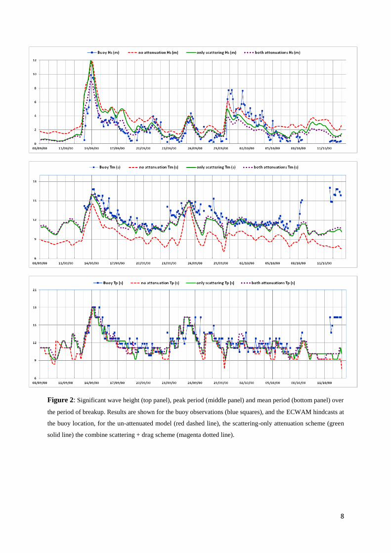
Figure 2 (a) to (c) compares the buoy observations to the model hindcasts, in terms of

significant wave height (top panel), peak period (middle panel) and mean period (bottom

panel). Because the sea ice cover at the buoy locations was always above 30%, the default

configuration of the model would simply not produce any waves at the buoy locations. We

also ran a case in which we modified the model to allow the waves to propagate freely in all

areas with ice concentration above 30% without any additional wind input, dissipation or

non-linear interaction (i.e. all source terms turned off). This is an unrealistic case, but it

serves as a baseline to study the impact of the attenuation scheme.

The results at the buoy location are plotted for the un-damped free propagation case, for the

scattering-only scheme and for both attenuation schemes (scattering + drag) combined. Prior

to the breakup, the wave model allows energy to propagate through the ice, whereas the buoy

indicates that the pack is still essentially unbroken, blocking the passage of any significant

7

wave energy. The pack ice broke up around the buoy on 14th September 2000 as large

amplitude storm waves approached the ice edge at the buoy location. During and after the

breakup, there is a reasonable correspondence between observations and the damped model

results. The model tracks the breakup event closely, though it does not reproduce the very

low wave heights (<1 m) observed by the buoy during subsequent calm periods.

Around the beginning of October, observed wave height shows significant variability which

is not followed by the model, though the observational data appear to be of good quality. It is

possible that small-scale variability in the forcing wind was not well captured by the

relatively coarse ERA-Interim forcing (80km horizontal resolution). In the final week of data

transmission, the buoy passed south of the 60% ice concentration contour and observed wave

height dropped to almost zero once more. This was not followed by the model, which

continued to allow waves to propagate to the buoy location in accordance with the ice

concentration remaining below 80%.

Mean period is well-tracked by both the attenuated models. The un-damped model always

exhibits too much high-frequency energy, though the form of the curve is well followed. Peak

wave periods are well tracked by both damped and undamped models. Adding the drag

attenuation reduces the corresponding wave heights slightly but improves the fit to observed

wave periods.

Wave spectra for selected times are shown in Figure 3 (a) to (f), again as measured at the

buoy as well as for un-damped and both attenuation schemes. The un-damped model

invariably has too much energy at high frequencies (at any frequency above the peak, in fact).

The damped models follow the spectral shape of the buoy measurements very well in most

cases, though the absolute amplitude is often a factor several times different from reality. The

model under-estimates the power of the most energetic events measured by the buoy,

probably due to the too-weak ERA-Interim winds, as previously mentioned.

8

Figure 2: Significant wave height (top panel), peak period (middle panel) and mean period (bottom panel) over

the period of breakup. Results are shown for the buoy observations (blue squares), and the ECWAM hindcasts at

the buoy location, for the un-attenuated model (red dashed line), the scattering-only attenuation scheme (green

solid line) the combine scattering + drag scheme (magenta dotted line).

9

Figure 3 (a) to (f): Frequency spectrum plots of buoy data and ECWAM hindcasts for selected times.

As for Figure 2, results are shown for the buoy (blue squares), the un-attenuated model (red dashed line),

the scattering only scheme (green solid line) the scattering + drag scheme (magenta dotted line). The

format used to write out the model spectra ignores small numbers, hence the apparent cut off in the

model spectra.

Figure 3 a) shows the situation just prior to the breakup (12th

September). As seen in the time

series, the model already has wave energy at this location, both un-damped and damped,

while the buoy has yet to experience any significant waves. Note the high-frequency peak at

f=0.36 Hz, suggesting local wave generation in open water or bobbing/rocking of the floe.

Following Czipott & Podney (1989), this frequency represents bobbing of a 0.2 m thick floe

or rocking of a 1.0 m thick floe, which is plausible. Figure 3 b) shows the situation at the

time of the breakup (14th

September). Both attenuated models represent the spectral peak

very well. Adding the ice bottom drag attenuation improves the fit to the tail of the spectrum

but slightly under-represents the peak power. Figure 3 c) is two days after the break up (17th

September). Some locally generated high frequency waves are visible in the attenuated model

simulations, since wave generation and dissipation are still active on the open water portion

of the grid box. Again the peak of the spectrum is well captured. Figure 3 d) (22nd

10

September) shows little change in the modelled spectra, while the buoy energy has dropped

back to the red noise spectrum (note that because of a limitation in the format of the output

model spectra, small model spectral density are truncated to zero, hence the apparent cut-off

in log-log plot). Figure 3 e) shows a case where the buoy wave height was well above any

modelled value (30th

September). Though the observed peak power is not achieved by the

model, the attenuated simulations show a good agreement for the high frequency tail. Finally,

Figure 3 f) is very near the end of the buoy life (12th

October), when the buoy observations

are once again significantly below the modelled results, close to the accelerometer’s noise

limit.

3.2 Effects of the damping scheme on waves outside the ice edge

The fit to the altimeter wave height data in the Southern Ocean (south of 50°S) is shown in

Table 1. Without sea ice attenuation the model exhibits a tendency to over-estimate wave

heights. With the attenuation included, the bias is largely removed and the overall fit to the

data improved. Also shown is the case where all waves are blocked if the sea ice

concentration is above 30% (as in the current operational ECWAM). Overall, using the

attenuation models gives similar statistical fit to the altimeter data around Antarctica.

Table 1: Comparison of the model first guess prior to assimilation of ERS-2 altimeter wave heights for all

observations south of 50°S from 26-08-2000 to 13-10-2000 in terms of bias (model – altimeter), root mean

square error (RMSE), Scatter Index (standard deviation of the difference normalised by the altimeter mean)

and Correlation Coefficient. Different standalone model configurations were used.

Number of

collocations = 19,860

No

attenuation

Attenuation

by

scattering

Both

attenuations

Full

blocking

for sea ice

cover >

30%

BIAS (m) 0.146 0.031 0.007 0.015

RMSE (m) 0.429 0.378 0.376 0.373

Scatter Index 0.106 0.098 0.097 0.097

Correlation

Coefficient 0.956 0.963 0.962 0.963

11

The characteristics of the wave field in open water near the ice edge are quite different

depending on which model is used, however. Comparing results between runs using both

schemes with the un-damped case demonstrates that the presence of the sea ice alters the

wave characteristics significantly, with an impact that extends far from the ice itself. The

effect of adding the attenuation by ice bottom drag in addition to the scattering scheme is

more confined to the ice edge.

In the current operational set-up, the impact of the sea ice is modelled by preventing all

waves in areas with sea ice concentration above 30%. The mean difference between the

enhanced attenuation model (using both attenuation mechanisms) and this operational

configuration is presented in Figure 4. While the differences are less drastic than the

comparison to the un-damped scheme, the influence of the sea ice is particularly visible

where lower wave heights and longer periods interact with the ice cover. Moreover, the

influence extends far down-wave of areas where the sea ice cover extends northwards.

The actual operational wave model at ECMWF is actively coupled to the atmospheric model

with a feedback of the waves on the wind. The WAM model was actually developed to

determine the sea state dependence of the air-sea fluxes. This feedback is linked to the actual

shape of the wave model spectra which controls the momentum exchange between the

atmosphere and the ocean (Janssen 2004, Janssen et al. 2002). Introducing this attenuation

model could therefore have an impact on the winds around the sea ice, further enhancing the

effect of sea ice on the waves.

12

Figure 4: The effect of implementing the full attenuation (scattering + drag) scheme of the current

study versus the present operational ECWAM (wave energy set to zero at ci >30%) in standalone

configuration. The effect is shown for both the mean SWH (left panel) and mean wave period (right

panel) from September 1st to October 13th, 2000. The black square indicates the position of the

buoy on the September 13th

and the red one on October 13th

.

3.3 Effects of the damping scheme in the context of the coupled IFS/ECWAM system

As discussed in the previous section, the high frequency part of the wave spectrum is affected

by the presence of sea ice. The influence extends some distance from the ice edge. The

modified model was tested in coupled mode, with an active feedback of the waves on the

atmosphere. We use the latest operational version of code and all experiments were carried

out in the context of continuous analysis cycles followed by 10 day forecasts every 12 hours.

This configuration is closely related to the configuration used by the operational high

resolution suite, except that the testing was done at about half the operational horizontal

resolution (~40 km for the atmosphere and ~55 km for the waves). The analysis is the best

estimate of the current state of the atmosphere, including ocean waves, obtained by blending

previous model estimate (first guess) with all available observations. As before, the only

information on sea ice is limited to sea ice cover as derived from the OSTIA (Donlon et al.

2011). The choice for the floe size distribution, the sea ice thickness and the ice-water drag

coefficient was kept as described above. No attempts were made to retune the schemes. Both

attenuation mechanisms are used. The experiments ran from 1 January 2012 to 31 March

2012.

13

Figure 5: The effect of implementing the full attenuation (scattering + drag) scheme of the

current study versus the present operational IFS/ECWAM coupled system. The effect is

shown for the mean SWH (top panels), the mean wave period (middle panels) and for the

10m neutral wind speed from January 1st to March 31th, 2012.

14

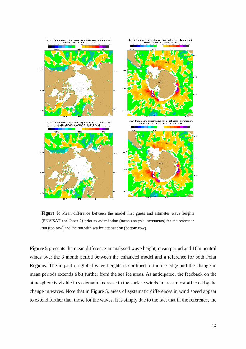
Figure 6: Mean difference between the model first guess and altimeter wave heights

(ENVISAT and Jason-2) prior to assimilation (mean analysis increments) for the reference

run (top row) and the run with sea ice attenuation (bottom row).

Figure 5 presents the mean difference in analysed wave height, mean period and 10m neutral

winds over the 3 month period between the enhanced model and a reference for both Polar

Regions. The impact on global wave heights is confined to the ice edge and the change in

mean periods extends a bit further from the sea ice areas. As anticipated, the feedback on the

atmosphere is visible in systematic increase in the surface winds in areas most affected by the

change in waves. Note that in Figure 5, areas of systematic differences in wind speed appear

to extend further than those for the waves. It is simply due to the fact that in the reference, the

15

wave parameters are only defined over areas with sea ice fraction less than 30% but the winds

are defined over all ocean points.

In these coupled runs, it appears that around Antarctica, analysed wave heights are

systematically over predicted (Figure 6). Adding the attenuation scheme in its present form

does not appear to have resolved the problem. Generally the fit to altimeter data (Table 2) is

similar in both simulations, with a small gain in the Arctic and a small deterioration in the

Antarctic. As an operational forecasting centre, ECMWF is primarily concerned with the

quality of its forecasts. The forecast errors can easily be assessed by comparing the

simulations to their respective analysis. The statistical analysis of these errors produces a

series of metrics (scores) that can be compared across the forecast range for different areas of

the world. For instance, the standard deviation of the error (with respect to the analysis) of

the two runs is compared in Figure 7 for significant wave height and in Figure 8 for 10m

wind speed over the oceans for both the Northern and Southern Hemispheres. There is a

marginally small degradation of the scores in the Northern Hemisphere for the run with

attenuation for both wave height and 10m wind. Note however that there is small increase in

standard deviation in those forecasts more in line with the analysis which could explain this

increase in errors. In the Southern Hemisphere, the scores are generally slightly better (wave

height) or statistically similar (winds).

Table 2: Comparison of the model first guess prior to assimilation of ENVISAT and Jason-2 altimeter

wave heights for all observations north of 40°N and south of 50°S from 01-01-2013 to 31-03-2013 in

terms of bias (model – altimeter), root mean square error (RMSE), Scatter Index (standard deviation of the

difference normalised by the altimeter mean) and Correlation Coefficient. Different coupled model

configurations were used.

reference

north of

40°N

Enhanced

model

north of

40°N

Reference

south of

50°S

Enhanced

model south of

50°S

Number of

observations 72664 72664 141497 141497

BIAS (m) -0.031 -0.034 0.041 0.045

RMSE (m) 0.421 0.419 0.347 0.351

Scatter Index 0.120 0.119 0.108 0.109

Correlation

Coefficient 0.966 0.966 0.962 0.962

16

Figure 7a: Significant wave height scores for the 10 day forecasts for the Northern Hemisphere. The

solid curve in the top left panel shows the normalised difference in standard deviation of forecast error

(STDE) in such a way that positive values indicate a lower STDE for the run with sea ice attenuation

(labelled NEW) than the reference run (labelled CONTROL). The normalisation was performed using

the mean of both runs. The vertical bars represent the confidence intervals at 95 percentile level. The top

right panel shows the actual difference in standard deviation of error for each forecast. The bottom left

panel is the mean STDE for both runs and the bottom right panel is the standard deviation of both

forecasts.

17

Figure 7b: same as Figure 7a but for the Southern Hemisphere.

Figure 7c: same as Figure 7a but 10m wind speed over the oceans.

18

Figure 7d: same as Figure 7c but for the Southern Hemisphere.

4. Discussion and conclusions

We have used unique field measurements of wave properties prior to, during and after

breakup at the Antarctic MIZ. We demonstrate that the enhanced ECWAM scheme provides

a reasonable match to the wave heights, periods and spectra measured at the buoy, using only

a simple look-up table for attenuation coefficient supplemented with a parameterisation of the

sea ice bottom drag. We acknowledge the simplistic nature of our parameterisation, but this is

deliberate since current operational models only have access to very basic sea ice

information, such as ice concentration data used here. Recognising that wave-ice interaction

might actually modify the wave spectral shape, we then applied the enhanced model to the

coupled atmosphere-wave model in a test configuration that resembles the one used in the

operational production of ECMWF high resolution 10 day forecasts. In such system, the

wave model feeds back sea-state dependent information on the air-sea fluxes, with the

potential of changing the atmospheric circulation. We found that the surface winds are

generally increased over the areas where waves and ice interacts. The forecast performances

are mixed and more tests will be needed to cover other seasons.

19

The model has no concept of floe breaking and thus transmits wave energy to the buoy long

before breakup actually occurs there. Since the scattering model is only applicable where the

ice is broken, coupling to a simple floe breaking model (such as that implemented by Dumont

et al., 2011 and Williams et al. 2013a) would be advantageous. Healing processes in the ice

cover, not included in the scheme, will also play a role. In fact, we should follow on the work

of the previous authors to add the coupling between the wave model and an ice model.

In the meantime, we limit the applicability of the wave propagation to the 0.3 – 0.8 ice

concentration range, as discussed. We note that other forms of ice edge can be modelled with

appropriate attenuation schemes (e.g. a viscous parameterisation for the vast frazil and

pancake zones of the advancing Antarctic sea ice cover, as demonstrated by de Carolis &

Desidiero (2002) and Wang and Shen (2010), with an appropriate switch in the model for the

advance/retreat season.

The conceptually simple model presented here simulates the observed parameters well,

however, smoothing the fluctuations in observed quantities and allowing the basic process of

energy loss will need to be followed. Working on the same ideas as in Williams et al. (2013),

we are planning to use the different components of the future forecasting system at ECMWF,

in which the atmosphere, the waves, the ocean and the sea ice are fully integrated into one

single system. On the one hand, sea ice information passed to the wave model would become

dynamic and would contain more comprehensive details on the ice condition. This will be a

welcome addition to the prescribed analysis of sea ice cover derived from satellite

observations which generally do not image small amounts of sea ice. On the other hand,

impact of waves on the mechanical straining of the ice can be modelled and passed back to

the ice model. We have developed a conceptual model which will use an estimate of the

mean square strain in the ice from the wave model to derive a probability of maximum strain

exceedance in the ice. Such a parameter should be used in the ice model to characterise the

ice strength. If successful, the aim is to run the model operationally – following extensive

validation - to define the location and width of the wave-influenced zone, and the major wave

parameters therein. This will provide valuable guidance for a wide range of scientific studies,

monitoring agencies and resource extraction operations.

20

Acknowledgements

We thank Alison Kohout (NIWA) for discussions regarding the attenuation coefficients in her

model, and the Alfred Wegener Institut für Polar- und Meeresforschung, Bremerhaven, for

the opportunity to work from F/S “Polarstern” during the field experiment and thank the

captain and crew for their kind cooperation. The field experiment was supported by the UK

Natural Environment Research Council, under grant “Short Timescale Motion of Pancake

Ice”, number GR3/12952. MJD was funded during the analysis and preparation of this paper

by the Office of Naval Research “Emerging Dynamics of the Marginal Ice Zone”

Departmental Research Initiative, and the “Arctic Climate Change, Economy and Society”

(ACCESS) project, grant number 265863 of the “Oceans 2010” call of the European Union

Seventh Framework Programme.

References

Ardhuin F., Tournadre J., Queffeulou P., Girard-Ardhuin F., Collard F., 2011. Observation

and parameterization of small icebergs: Drifting breakwaters in the southern ocean.

Ocean Modelling, 39, 405-410.

Asplin, M. G., R. Galley, D. G. Barber, and S. Prinsenberg (2012), Fracture of summer

perennial sea ice by ocean swell as a result of Arctic storms, J. Geophys. Res. 117,

C06025, doi:10.1029/2011JC007221.

Barber, D.G., Galley, R., Asplin, M.G., de Abreu, R., Warner, K-A., Pućko, M., Gupta, M.,

Prinsenberg, S. and S. Julien, 2009. Perennial pack ice in the southern Beaufort Sea

was not as it appeared in the summer of 2009, Geophys. Res. Lett., 36, L24501,

doi:10.1029/2009GL041434.

Bennetts, L.G. and Squire, V. A., 2012 a. On the calculation of an attenuation coefficient for

transects of ice-covered ocean, Royal Society of London Proceedings Series A, 468,

136-162, doi :10.1098/rspa.2011.0155.

Bennetts, L.G. and Squire, V. A., 2012 b. Model sensitivity analysis of scattering-induced

attenuation of ice-coupled wave. Ocean Modelling, 45-46, 0-13.

Bidlot J.-R. 2012: Present status of wave forecasting at ECMWF. Proceeding from the

ECMWF Workshop on Ocean Waves, 25-27 June 2012.

Broström, G. and Christensen, K. H., 2008: Waves and sea ice, report 5/2008, Norwegian

Meteorological Institute (http://met.no/Publikasjoner+2008.b7C_wlfY47.ips)

21

Czipott, P.V. and W.N. Podney, 1989. Measurements of fluctuations in tilt of Arctic ice at the

CEAREX oceanography camp: Experiment review, data catalog and preliminary

results. Final tech. report N00014-89-C-0087, U.S. Navy, Washington D.C.

De Carolis, G. and D. Desidiero, 2002. Dispersion and attenuation of gravity waves in ice: a

two-layer viscous model with experimental data validation. Phys. Lett. A, 305, 399-

412.

Dee, D. P., and 36 others, 2011. The ERA-Interim reanalysis: configuration and performance

of the data assimilation system. Q.J.R. Meteorol. Soc., 137, 553–597.

doi: 10.1002/qj.828

Doble, M.J., Coon, M. D. and P. Wadhams, 2003. Pancake ice formation in the Weddell Sea,

J. Geophys. Res. 108(C7), 3209. doi: 10.1029/2002JC001373

Doble, M.J., and J.-R. Bidlot, 2013. Wave buoy measurements at the Antarctic sea ice edge

compared with an enhanced ECMWF WAM: Progress towards global waves-in-ice

modelling. Ocean Modell. 70, 166-173.

Donlon, C. J., M. Martin, J. D. Stark, J. Roberts-Jones, E. Fiedler and W. Wimmer, 2011.

The Operational Sea Surface Temperature and Sea Ice analysis (OSTIA). Remote

Sensing of the Environment. doi: 10.1016/j.rse.2010.10.017 2011.

Dumont, D., A. Kohout, and L. Bertino, 2011. A wave-based model for the marginal ice zone

including a floe breaking parameterization, J. Geophys. Res., 116, C04001,

doi:10.1029/2010JC006682.

Francis, O.P., Panteleev, G.G. and D.E. Atkinson, 2011. Ocean wave conditions in the

Chukchi Sea from satellite and in situ observations. Geophs. Res. Lett. 38, L24610,

doi:10.1029/2011GL049839

Fox, C., and T. G. Haskell, 2001. Ocean wave speed in the Antarctic MIZ. Annals of

Glaciology, 33.

Janssen, P. 2004. The Interaction of Ocean Waves and Wind. Cambridge University Press,

308+viii pp.

Janssen, P.A.E.M., J.D. Doyle, J. Bidlot, B. Hansen, L. Isaksen and P. Viterbo, 2002: Impact

and feedback of ocean waves on the atmosphere. in Advances in Fluid Mechanics,

Atmosphere-Ocean Interactions, Vol. I, WITpress, Ed. W.Perrie. 155-197.

Kohout, A.L. and M.H. Meylan, 2008. An elastic plate model for wave attenuation and ice

floe breaking in the marginal ice zone. J. Geophys. Res. 113, C09016,

doi:10.1029/2007JC004434.

22

Kohout, A.L. and M. H Meylan and D. R. Plew, 2011.Wave attenuation in a marginal ice

zone due to the bottom roughness of ice floes. Annals Glaciology, 52(57), 118—122.

Krinner, G., Rinke, A, Dethloff, K. and I.V. Gorodetskaya, 2010. Impact of prescribed Arctic

sea ice thickness in simulations of the present and future climate. Climate Dynamics

35, 619-633

Lange, M. A., Ackley, S.F., and P. Wadhams, 1989. Development of sea ice in the Weddell

Sea, Ann. Glaciol., 12, 92–96.

Masson D. and P. H. LeBlond, 1989. Spectral Evolution of Wind-Generated Surface Gravity

Waves in a Dispersed Ice Field. J. Fluid Mech., 202, 111-136.

Perrie, W., and Y. Hu, 1996. Air-ice-ocean momentum exchange, part 1: energy transfer

between waves and ice floes . J. Phys. Oceanog. 26, 1705-1720.

Perovich, D. K., Richter-Menge, J.A., Jones, K.F., and B. Light, 2008. Sunlight, water, and

ice: Extreme Arctic sea ice melt during the summer of 2007, Geophys. Res. Lett., 35,

L11501, doi:10.1029/2008GL034007

Polnikov, V. G., and I. V. Lavrenov, 2007. Calculation of the nonlinear energy transfer

through the wave spectrum at the sea surface covered with broken ice. Oceanology,

47, 334-343.

Steele, M., 1992. Sea ice melting and floe geometry in a simple ice-ocean model. J. Geophys.

Res. 97(C11), 17,729-17,738.

Steer, A., Worby, A.P. and P. Heil, 2008. Observed changes in sea-ice floe size distribution

during early summer in the western Weddell Sea. Deep-Sea Research Part II, 55,

933-942.

Squire, V. A., 2007. Of ocean waves and sea-ice revisited, Cold. Reg. Sci. Tech., 49, 110–

133.

Squire, V.A., Dugan, J.P., Wadhams, P., Rottier, P.J., and A.K. Liu, 1995. Of ocean waves

and sea ice. Annual Review of Fluid Mechanics 27, 115-168.

Toyota, T., Haas, C. and T. Tamura, 2011. Size distribution and shape properties of relatively

small sea-ice floes in the Antarctic marginal ice zone in late winter, Deep Sea Res. II,

doi:10.1016/j.dsr2.2010.10.034.

Vaughan, G.L. and V.A. Squire, 2011. Wave induced fracture probabilities for Arctic sea ice.

Cold Reg. Sci. Tech. 67, 31-36.

Wadhams, P., Squire, V.A., Goodman, D.J., Cowan, A.M. and S. C. Moore, 1988. The

attenuation rates of ocean waves in the marginal ice zone, J. Geophys. Res., 93(C6),

6799–6818.

23

Wang, R., Shen, H. H., 2010: Gravity waves propagating into ice covered ocean: A

viscoelastic model. J. Geophys. Res., 115 (C06024), DOI: 10.1029/2009JC005591

Williams, T., Bennetts, L., Dumont, D. Squire, V. and Bertino, L., 2013a. Wave-ice

interactions in the marginal ice zone. Part 1: Theoretical foundations. Ocean Modell.

in press

Williams, T., Bennetts, L., Dumont, D. Squire, V. and Bertino, L., 2013b. Wave-ice

interactions in the marginal ice zone. Part 2: Numerical implementation and

sensitivity studies along 1D transects of the ocean surface. Ocean Modell. in press.