income approach - ted whitmer flows are developed vertically from potential gross income to net...
TRANSCRIPT

INCOME APPROACH
Direct Cap ! Yield Cap ! Rate Relationships
Income © Ted Whitmer, All Rights Reserved.
2"
Chapter 46 Operating Statements & Reconstruction
Overview
The following are financial statements for income properties. " Income statement " Balance sheet " Cash flow statement " Rent roll " Capital expenditure plan " Projected budgets
In addition, an appraiser could benefit from…
" Leases " Environmental & structural reports " Plans & specifications " Cost information " Current & past contracts on the property " Any listing information " HUD statements from any sales of the property " Title policies
Financial statements are a way to keep score in a business. They also serve as the starting point for many financial and management decisions. In addition, financing is easier when financial statements are healthy. Bankers look at the following statements when considering an applicant for a loan. Effective managers periodically look at the statements of a firm to adjust to market conditions. Financial statements should also be compared to industry averages. Often managers of companies find that there income statement looks healthy, their balance sheet looks acceptable, but they never seem to have enough cash to pay bills as they come due. Cash flow is often a problem when the average length of time to collect receivables is longer than average time of payables. Cash flow can be improved by extending payables and/or by shortening average collections. Cash flow is particularly a problem during expansion. Especially when employees are paid by salary or on a draw basis. Additionally, growing firms must pay for additional lease space, equipment, other capital expenditures and training. However, it is generally a long time before a new employee is productive with his/her first billings. Working capital is money needed in a firm to pay bills as they come due. Although working capital is used to pay short-term debt, it is a long-tern investment. For example, if a new firm has 60 days of bills that total $30,000 and no collections. The amount of $30,000 is needed to start the business. Once money comes in, a portion of the owner's salary or profit can be used to payoff the debt created by the gap. Otherwise, a continual
Income © Ted Whitmer, All Rights Reserved.
3"
line of credit to pay bills may be established and the firm pays interest on the debt. As the firm expands additional working capital is needed. A large firm may have as much as $100,000 in working capital that is engaged either through debt or equity. The working capital may be recovered through closing the firm, a sale of the firm, or some by contraction.
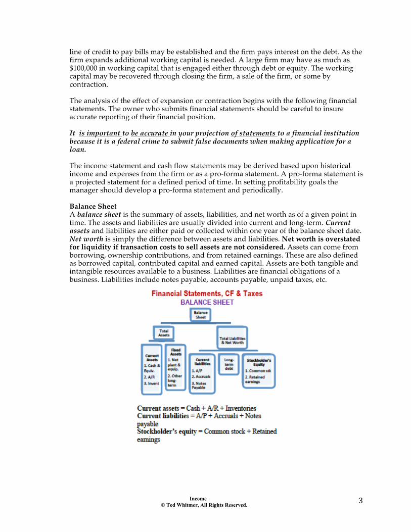
The analysis of the effect of expansion or contraction begins with the following financial statements. The owner who submits financial statements should be careful to insure accurate reporting of their financial position. It is important to be accurate in your projection of statements to a financial institution because it is a federal crime to submit false documents when making application for a loan. The income statement and cash flow statements may be derived based upon historical income and expenses from the firm or as a pro-forma statement. A pro-forma statement is a projected statement for a defined period of time. In setting profitability goals the manager should develop a pro-forma statement and periodically. Balance Sheet A balance sheet is the summary of assets, liabilities, and net worth as of a given point in time. The assets and liabilities are usually divided into current and long-term. Current assets and liabilities are either paid or collected within one year of the balance sheet date. Net worth is simply the difference between assets and liabilities. Net worth is overstated for liquidity if transaction costs to sell assets are not considered. Assets can come from borrowing, ownership contributions, and from retained earnings. These are also defined as borrowed capital, contributed capital and earned capital. Assets are both tangible and intangible resources available to a business. Liabilities are financial obligations of a business. Liabilities include notes payable, accounts payable, unpaid taxes, etc.
Income © Ted Whitmer, All Rights Reserved.
4"
Balance Sheet
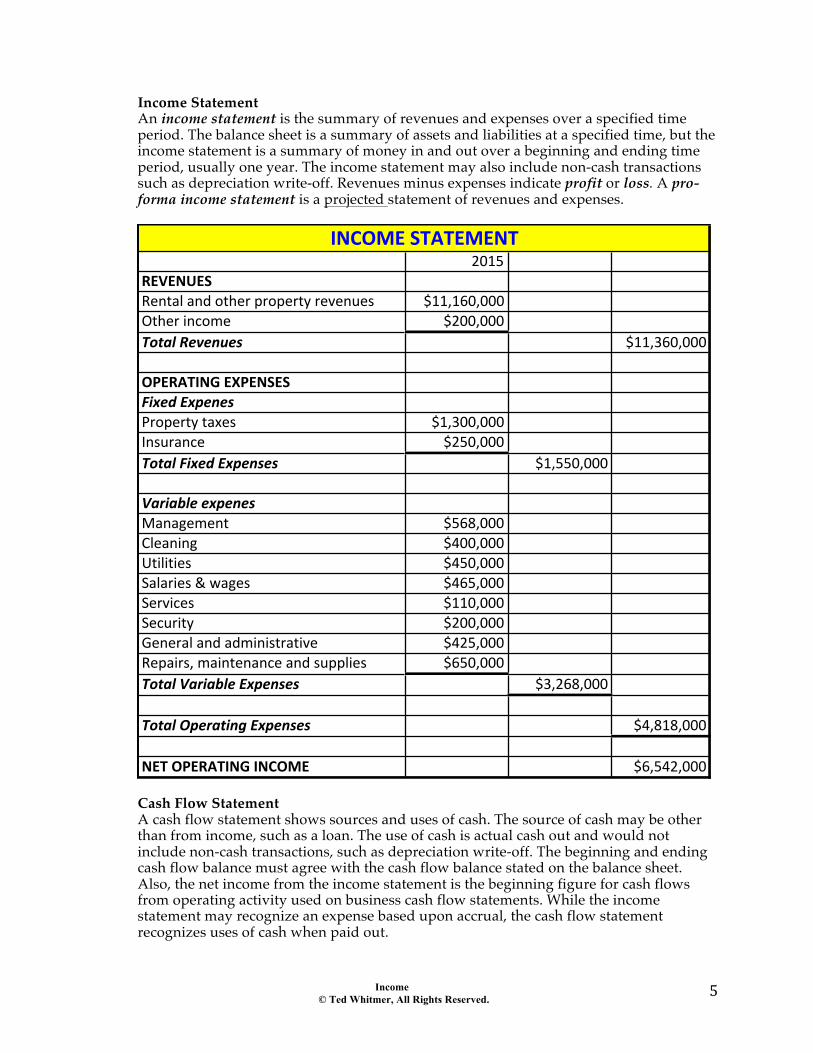
Business Personal Assets: $ Assets: $ 1. Cash on hand $ 1. Cash on hand $ 2. Cash in bank $ 2. Cash in bank $ 3. US government securities $ 3. US government securities $ 4. Other marketable securities $ 4. Other marketable securities $ 5. Notes receivable $ 5. Notes receivable $ 6. Accounts receivable $ 6. Accounts receivable $ 7. Other liquid asset $ 7. Other liquid asset $ 8. Other liquid asset $ 8. Other liquid asset $ TOTAL CURRENT ASSETS $ TOTAL CURRENT ASSETS $
9. Real estate owned $ 9. Real estate owned $ 10. Mortgages owned $ 10. Mortgages owned $ 11. Contracts owned $ 11. Contracts owned $ 12. Notes & accounts receivable doubtful
$ 12. Notes & accounts receivable doubtful
$
13. Notes - Friends/family $ 13. Notes - Friends/family $ 14. Other securities $ 14. Other securities $ 15. Furniture, fixtures & equipment $ 15. Furniture, fixtures & equipment $ 16. Automobiles $ 16. Automobiles $ 17. Other asset $ 17. Motorcycles, boats, recreational,
etc. $
18. Other asset $ 18. Other asset $ 19. Other asset $ 19. Other asset $ 20. Other asset $ 20. Other asset $ TOTAL LONG-TERM ASSETS $ TOTAL LONG-TERM ASSETS $ TOTAL ASSETS $ TOTAL ASSETS $
Liabilities: $ Liabilities: $ 1. Notes due banks $ 1. Notes due banks $ 2. Notes due relatives/friends $ 2. Notes due relatives/friends $ 3. Notes due others $ 3. Notes due others $ 4. Accounts & bills payable $ 4. Accounts & bills payable $ 5. Unpaid federal income taxes $ 5. Unpaid federal income taxes $ 6. Unpaid state & local taxes $ 6. Unpaid state & local taxes $ 7. Interest & other payments due $ 7. Interest & other payments due $ 8. Any other past dues $ 8. Any other past dues $ 9. Other short-term liability $ 9. Other short-term liability $ 10. Other short-term liability $ 10. Other short-term liability $ 11. Notes due on real estate $ 11. Notes due on real estate $ 12. Credit card balances $ 12. Credit card balances $ 13. Contingent debt $ 13. Contingent debt $ 14. Other liabilities $ 14. Other liabilities $ 15. Other liabilities $ 15. Other liabilities $ 16. Other liabilities $ 16. Other liabilities $ TOTAL LIABILITIES $ TOTAL LIABILITIES $
NET WORTH $ NET WORTH $ (Assets minus liabilities) (Assets minus liabilities)
Income © Ted Whitmer, All Rights Reserved.
5"
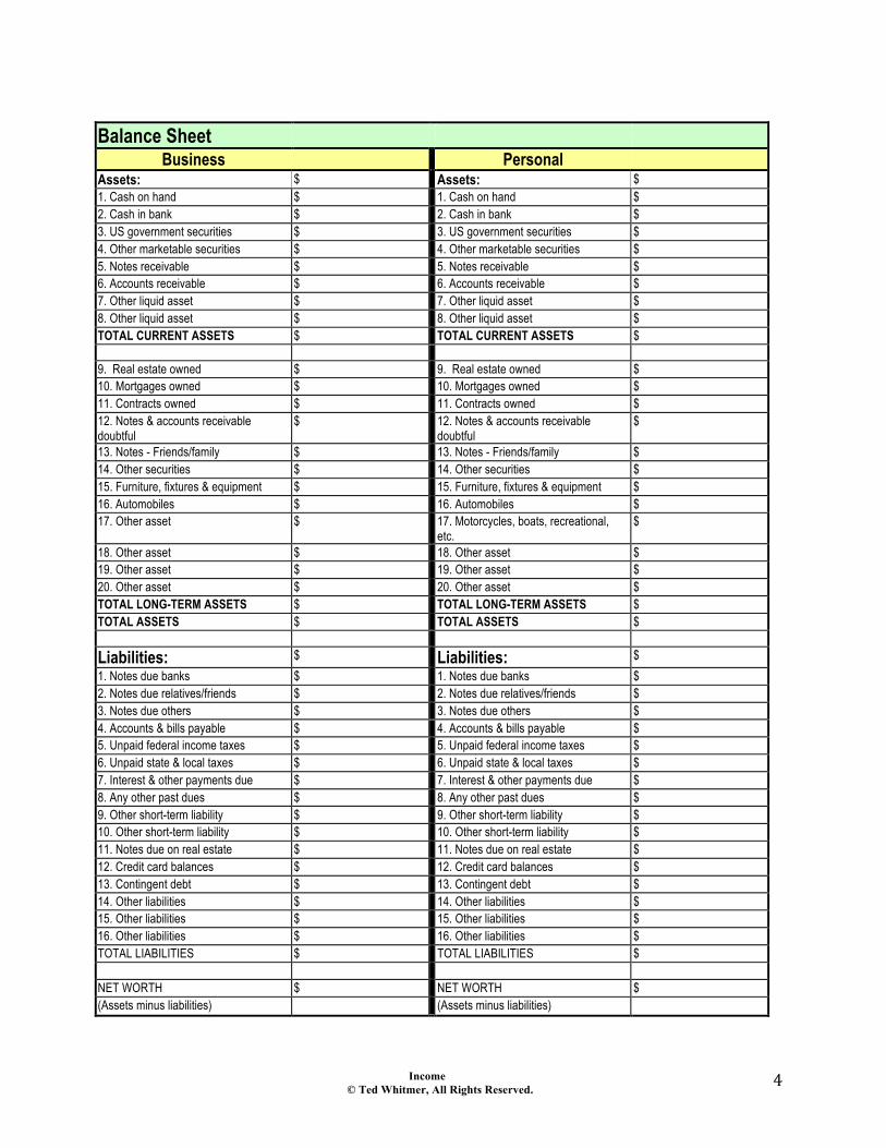
Income Statement An income statement is the summary of revenues and expenses over a specified time period. The balance sheet is a summary of assets and liabilities at a specified time, but the income statement is a summary of money in and out over a beginning and ending time period, usually one year. The income statement may also include non-cash transactions such as depreciation write-off. Revenues minus expenses indicate profit or loss. A pro-forma income statement is a projected statement of revenues and expenses.
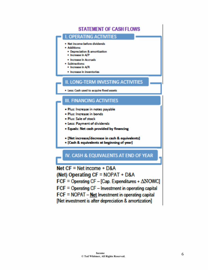
Cash Flow Statement A cash flow statement shows sources and uses of cash. The source of cash may be other than from income, such as a loan. The use of cash is actual cash out and would not include non-cash transactions, such as depreciation write-off. The beginning and ending cash flow balance must agree with the cash flow balance stated on the balance sheet. Also, the net income from the income statement is the beginning figure for cash flows from operating activity used on business cash flow statements. While the income statement may recognize an expense based upon accrual, the cash flow statement recognizes uses of cash when paid out.
2015REVENUESRental+and+other+property+revenues $11,160,000Other+income $200,000Total&Revenues $11,360,000
OPERATING-EXPENSESFixed&ExpenesProperty+taxes $1,300,000Insurance $250,000Total&Fixed&Expenses $1,550,000
Variable&expenesManagement $568,000Cleaning $400,000Utilities $450,000Salaries+&+wages $465,000Services $110,000Security $200,000General+and+administrative $425,000Repairs,+maintenance+and+supplies $650,000Total&Variable&Expenses $3,268,000
Total&Operating&Expenses $4,818,000
NET-OPERATING-INCOME $6,542,000
INCOME-STATEMENT
Income © Ted Whitmer, All Rights Reserved.
6"
Income © Ted Whitmer, All Rights Reserved.
7"
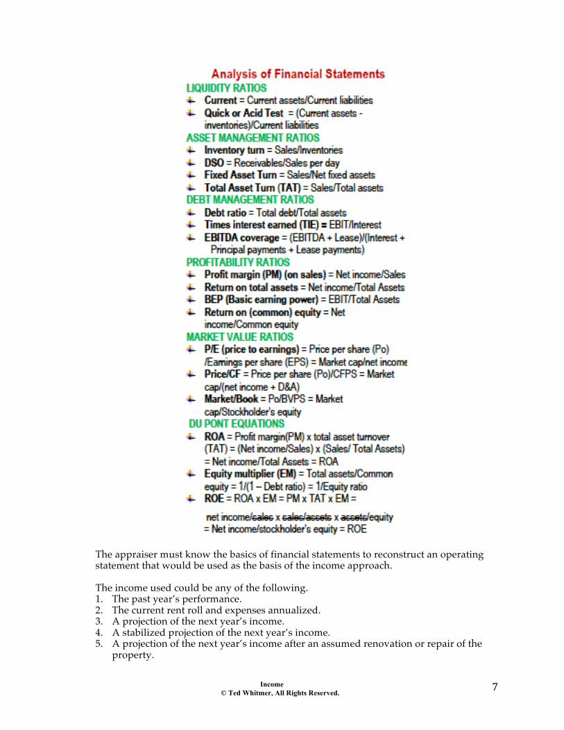
The appraiser must know the basics of financial statements to reconstruct an operating statement that would be used as the basis of the income approach. The income used could be any of the following. 1. The past year’s performance. 2. The current rent roll and expenses annualized. 3. A projection of the next year’s income. 4. A stabilized projection of the next year’s income. 5. A projection of the next year’s income after an assumed renovation or repair of the
property.
Income © Ted Whitmer, All Rights Reserved.
8"
6. A projection based upon normalizing rent and/or expenses based upon the appraiser’s estimate of what “competent management” would consider reasonable.
7. An income projection with or without reserves, tenant improvements & leasing commissions.
The appraiser should project the income statement based upon the market. (However, some markets lack a consistent way to develop a projected income statement.) Many market participants buy properties based upon the year before performance and not on a projected income statement. This does not violate the theory of anticipation. The anticipation is built into the capitalization rate instead of the income. One market participant remarked “I’m not paying them for my expertise. I expect to increase the net income, but am paying for the property based upon what they were able to do.” Many appraisal courses teach to use a projected income statement for the subject. Then the appraiser is instructed to force that upon their sales information. It would be preferable to see if there is a consistent way the market projects the income statement, then do the same for the subject. For example, if the sales show a consistent capitalization rate based upon projected income that does not include reserves, leasing commissions and tenant improvements, then do the same with the subject. If there is a more consistent capitalization rate with the reserves, leasing commissions and tenant improvements “above the line”, then put those categories into the calculation of net operating income. The point is to derive this from the market. A number of services providing yield and capitalization rates were surveyed. Some respondents put tenant improvements and leasing commissions above the line and some include the expenses below the line. “Above the line” means the categories are included as an expense line before net operating income is calculated. “Below the line” means the expenditures for tenant improvements and leasing commissions are not used in the calculation of net operating income.
Income © Ted Whitmer, All Rights Reserved.
9"
Chapter 47 Projecting Cash Flows & Reversion
Overview
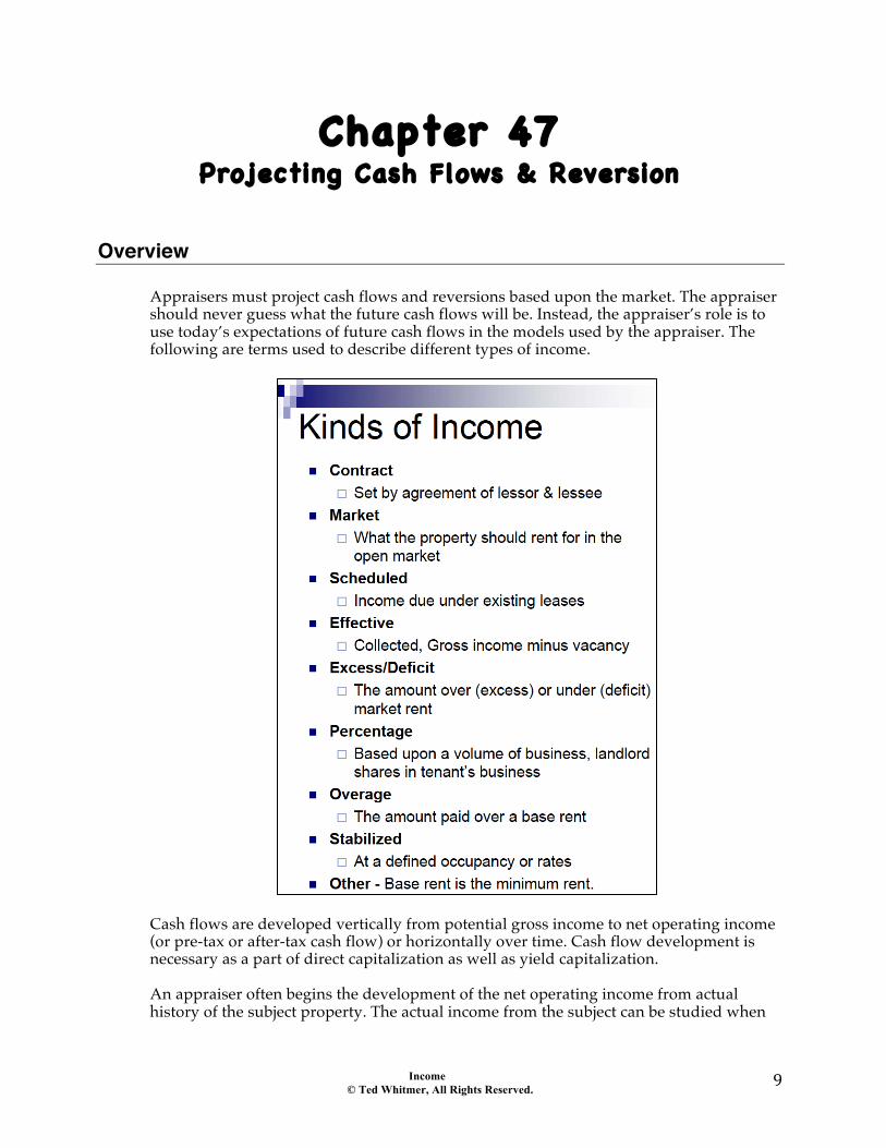
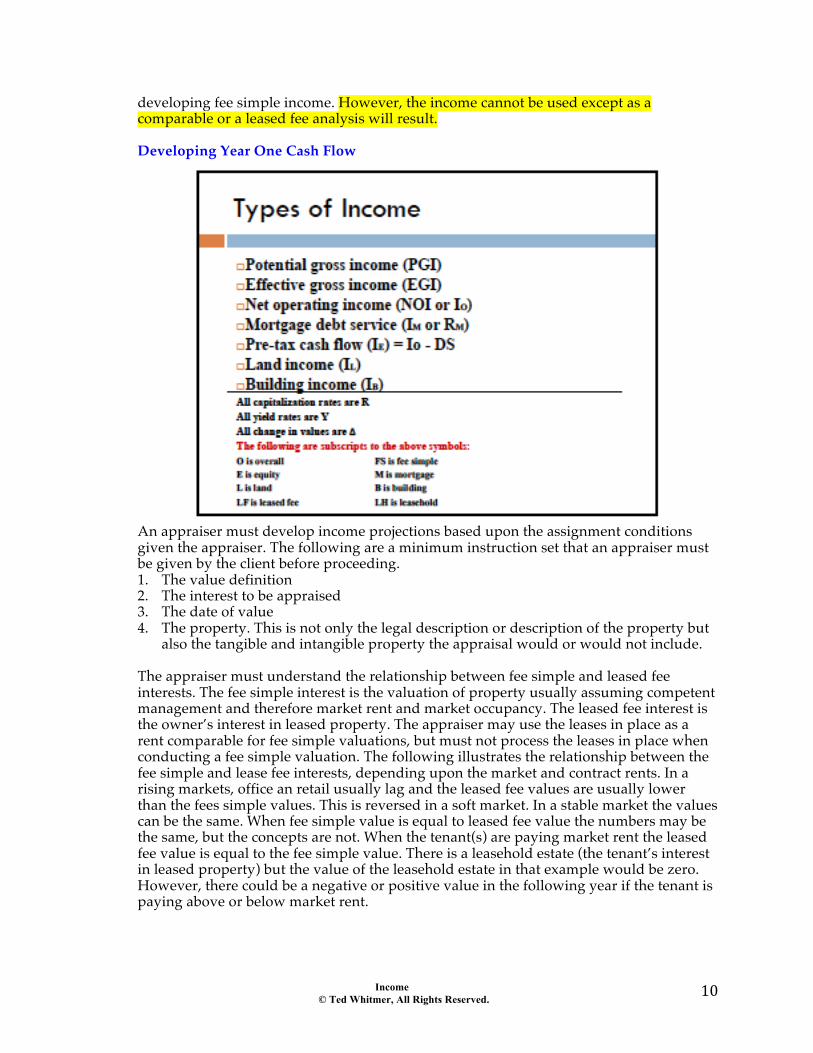
Appraisers must project cash flows and reversions based upon the market. The appraiser should never guess what the future cash flows will be. Instead, the appraiser’s role is to use today’s expectations of future cash flows in the models used by the appraiser. The following are terms used to describe different types of income.
Cash flows are developed vertically from potential gross income to net operating income (or pre-tax or after-tax cash flow) or horizontally over time. Cash flow development is necessary as a part of direct capitalization as well as yield capitalization. An appraiser often begins the development of the net operating income from actual history of the subject property. The actual income from the subject can be studied when
Income © Ted Whitmer, All Rights Reserved.
10"
developing fee simple income. However, the income cannot be used except as a comparable or a leased fee analysis will result. Developing Year One Cash Flow
An appraiser must develop income projections based upon the assignment conditions given the appraiser. The following are a minimum instruction set that an appraiser must be given by the client before proceeding. 1. The value definition 2. The interest to be appraised 3. The date of value 4. The property. This is not only the legal description or description of the property but
also the tangible and intangible property the appraisal would or would not include.
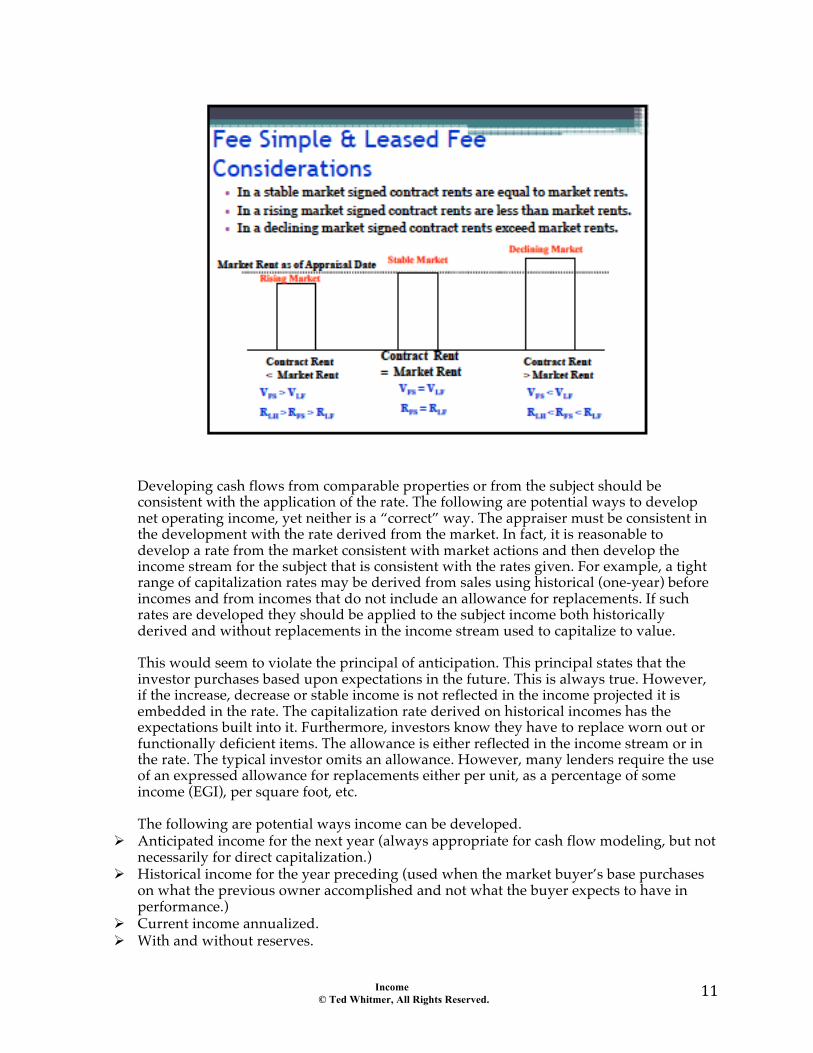
The appraiser must understand the relationship between fee simple and leased fee interests. The fee simple interest is the valuation of property usually assuming competent management and therefore market rent and market occupancy. The leased fee interest is the owner’s interest in leased property. The appraiser may use the leases in place as a rent comparable for fee simple valuations, but must not process the leases in place when conducting a fee simple valuation. The following illustrates the relationship between the fee simple and lease fee interests, depending upon the market and contract rents. In a rising markets, office an retail usually lag and the leased fee values are usually lower than the fees simple values. This is reversed in a soft market. In a stable market the values can be the same. When fee simple value is equal to leased fee value the numbers may be the same, but the concepts are not. When the tenant(s) are paying market rent the leased fee value is equal to the fee simple value. There is a leasehold estate (the tenant’s interest in leased property) but the value of the leasehold estate in that example would be zero. However, there could be a negative or positive value in the following year if the tenant is paying above or below market rent.
Income © Ted Whitmer, All Rights Reserved.
11"
Developing cash flows from comparable properties or from the subject should be consistent with the application of the rate. The following are potential ways to develop net operating income, yet neither is a “correct” way. The appraiser must be consistent in the development with the rate derived from the market. In fact, it is reasonable to develop a rate from the market consistent with market actions and then develop the income stream for the subject that is consistent with the rates given. For example, a tight range of capitalization rates may be derived from sales using historical (one-year) before incomes and from incomes that do not include an allowance for replacements. If such rates are developed they should be applied to the subject income both historically derived and without replacements in the income stream used to capitalize to value. This would seem to violate the principal of anticipation. This principal states that the investor purchases based upon expectations in the future. This is always true. However, if the increase, decrease or stable income is not reflected in the income projected it is embedded in the rate. The capitalization rate derived on historical incomes has the expectations built into it. Furthermore, investors know they have to replace worn out or functionally deficient items. The allowance is either reflected in the income stream or in the rate. The typical investor omits an allowance. However, many lenders require the use of an expressed allowance for replacements either per unit, as a percentage of some income (EGI), per square foot, etc. The following are potential ways income can be developed.
# Anticipated income for the next year (always appropriate for cash flow modeling, but not necessarily for direct capitalization.)
# Historical income for the year preceding (used when the market buyer’s base purchases on what the previous owner accomplished and not what the buyer expects to have in performance.)
# Current income annualized. # With and without reserves.
Income © Ted Whitmer, All Rights Reserved.
12"
# With and without repairs and other curables. # Actual occupancy or stabilized or some other occupancy. # ETC., ETC., ETC.
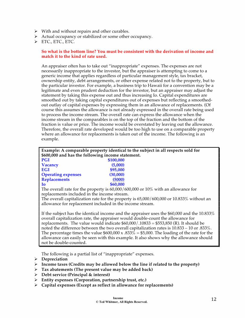
So what is the bottom line? You must be consistent with the derivation of income and match it to the kind of rate used. An appraiser often has to take out “inappropriate” expenses. The expenses are not necessarily inappropriate to the investor, but the appraiser is attempting to come to a generic income that applies regardless of particular management style, tax bracket, ownership entity, debt arrangements, or other expense related not to the property, but to the particular investor. For example, a business trip to Hawaii for a convention may be a legitimate and even prudent deduction for the investor, but an appraiser may adjust the statement by taking this expense out and thus increasing Io. Capital expenditures are smoothed out by taking capital expenditures out of expenses but reflecting a smoothed-out outlay of capital expenses by expressing them in an allowance of replacements. (Of course this assumes the allowance is not already expressed in the overall rate being used to process the income stream. The overall rate can express the allowance when the income stream in the comparables is on the top of the fraction and the bottom of the fraction is value or price. The income would be overstated by leaving out the allowance. Therefore, the overall rate developed would be too high to use on a comparable property where an allowance for replacements is taken out of the income. The following is an example. Example: A comparable property identical to the subject in all respects sold for $600,000 and has the following income statement. PGI $100,000 Vacancy (5,000) EGI $95,000 Operating expenses (30,000) Replacements (5000) Io $60,000 The overall rate for the property is 60,000/600,000 or 10% with an allowance for replacements included in the income stream. The overall capitalization rate for the property is 65,000/600,000 or 10.833% without an allowance for replacement included in the income stream. If the subject has the identical income and the appraiser uses the $60,000 and the 10.833% overall capitalization rate, the appraiser would double-count the allowance for replacements. The value would indicate $60,000/.10833 = $553,850 (R). It should be noted the difference between the two overall capitalization rates is 10.833 – 10 or .833%. The percentage times the value $600,000 x .833% = $5,000. The loading of the rate for the allowance can easily be seen with this example. It also shows why the allowance should not be double-counted. The following is a partial list of “inappropriate” expenses.
# Depreciation # Income taxes (Credits may be allowed below the line if related to the property) # Tax abatements (The present value may be added back) # Debt service (Principal & interest) # Entity expenses (Corporation, partnership trust, etc.) # Capital expenses (Except as reflect in allowance for replacements)
Income © Ted Whitmer, All Rights Reserved.
13"
# Travel expenses (Some related directly to the property could be alright) # Business expenses (Related to the business and not the real estate) # Excessive expenses (These would be the correct category, but are not within market
guidelines) The following are ways to estimate allowance for replacements.
# Per unit (# units x $per unit for replacements) # Per square foot (square foot x $ PSF for replacements) # As a percentage of effective or potential gross income (Income x % set aside for
replacements) # By dividing the cost of a replacement item by the useful life (straight-line, this
assumes the increase in the cost of the item is offset by money that can be earned from investing the funds)
# By multiplying the cost of a replacement item by the sinking fund factor for the useful life of the item (This assumes either (1) the money could be set aside growing interest, (2) the cost of the item used is the anticipated cost in the future and this gives credit to the cash set aside, (3) the typical investor does not set aside money for replacements, but borrows when it is time to replace. Therefore, the sinking fund rate is the difference between the opportunity cost and the borrow rate.)
Income © Ted Whitmer, All Rights Reserved.
14"
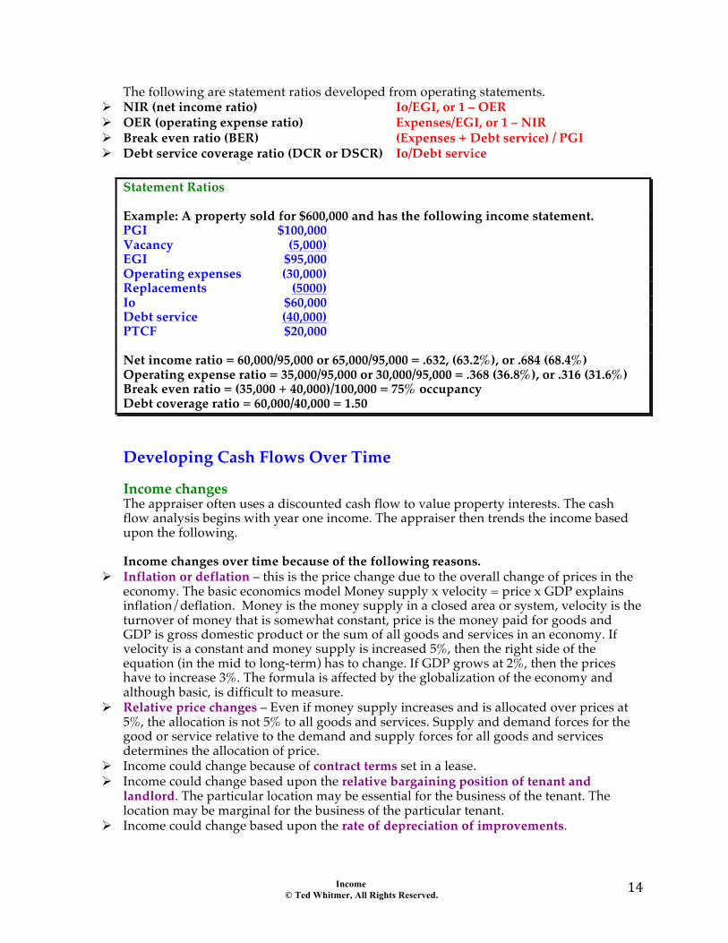
The following are statement ratios developed from operating statements. # NIR (net income ratio) Io/EGI, or 1 – OER # OER (operating expense ratio) Expenses/EGI, or 1 – NIR # Break even ratio (BER) (Expenses + Debt service) / PGI # Debt service coverage ratio (DCR or DSCR) Io/Debt service
Statement Ratios Example: A property sold for $600,000 and has the following income statement. PGI $100,000 Vacancy (5,000) EGI $95,000 Operating expenses (30,000) Replacements (5000) Io $60,000 Debt service (40,000) PTCF $20,000 Net income ratio = 60,000/95,000 or 65,000/95,000 = .632, (63.2%), or .684 (68.4%) Operating expense ratio = 35,000/95,000 or 30,000/95,000 = .368 (36.8%), or .316 (31.6%) Break even ratio = (35,000 + 40,000)/100,000 = 75% occupancy Debt coverage ratio = 60,000/40,000 = 1.50 Developing Cash Flows Over Time Income changes The appraiser often uses a discounted cash flow to value property interests. The cash flow analysis begins with year one income. The appraiser then trends the income based upon the following. Income changes over time because of the following reasons.
# Inflation or deflation – this is the price change due to the overall change of prices in the economy. The basic economics model Money supply x velocity = price x GDP explains inflation/deflation. Money is the money supply in a closed area or system, velocity is the turnover of money that is somewhat constant, price is the money paid for goods and GDP is gross domestic product or the sum of all goods and services in an economy. If velocity is a constant and money supply is increased 5%, then the right side of the equation (in the mid to long-term) has to change. If GDP grows at 2%, then the prices have to increase 3%. The formula is affected by the globalization of the economy and although basic, is difficult to measure.
# Relative price changes – Even if money supply increases and is allocated over prices at 5%, the allocation is not 5% to all goods and services. Supply and demand forces for the good or service relative to the demand and supply forces for all goods and services determines the allocation of price.
# Income could change because of contract terms set in a lease. # Income could change based upon the relative bargaining position of tenant and
landlord. The particular location may be essential for the business of the tenant. The location may be marginal for the business of the particular tenant.
# Income could change based upon the rate of depreciation of improvements.
Income © Ted Whitmer, All Rights Reserved.
15"
# Income could change because the tenant is improving the property. The landlord may not look for increases if the tenant improves the property during the tenancy. Value changes The appraiser often derives a future value (reversion) as a component of a discounted cash flow. A reversion is a future value. That is why the term “the present value of the reversion” is used. If the property is a sell-out type property such as a subdivision, condominium project, time-share, etc. the hoped for reversion by a developer/investor is $0. If the property is a retail center, office building, residential property, or industrial, commercial property the reversion is hoped to be some future value, even if just land value. The following are types of reversions (note all are future values)
# Property –sale price less costs of sale # Equity – property reversion less remaining loan balance # Mortgage – the loan balance as of the date of sale # Land – the value of the land at the date of sale. Because land is often a negative carry (the
expenses exceed the rental income), the land must outpace inflation to produce a good return. The bottom line is the land has to have a change of highest and best use or the ultimate highest and best use must come about.
# Building – the value of the building as of the date of sale. The reversion to the building is affected by the following.
o Depreciation on the building, e.g. 2%/year o Inflation in building costs, e.g. 4%/year o Increasing rate of return required to the building (in general the older the building, the
higher the rate of return. o Changes in tax laws

Income © Ted Whitmer, All Rights Reserved.
16"
Chapter 48 Stabilizing Cash Flows
Overview
There are numerous reasons to stabilize cash flows. The following is a partial list of those reasons. 1. The property is below market or stabilized occupancy because the market is soft. 2. The property is below market or stabilized occupancy because it is new. 3. The property is below market or stabilized occupancy because it has poor
management. 4. The property is below market or stabilized occupancy because there happened to be a
significant move-out of a major tenant or many tenants. 5. The property is below market or stabilized occupancy because it is being renovated. 6. Leases are not at market for some reason. 7. Leases have a structure that must be normalized to properly compare to another
structure. An example of this is when a comparable has increases built into the lease but the subject is being analyzed for long-term and level leases. The income must be stabilized to properly compare to the subject structure.
An example of an income stabilizing factor is a K-factor. The K-factor gives equivalent level income for an income stream that changes constant ratio. It is not a present value factor, but instead is used to smooth out streams that change constant ratio. Example: An income stream starts at $10,000 and increases 4%/year for 5 years and the yield rate is 10%. What is the equivalent level income and what is the K-factor? 1.04 Enter Enter Enter 10,000 g CFj X g CFj X g CFj X g CFj X g CFj 10 I f NPV [40,759] 5 N solve PMT [10,752.13] K-factor: 10,752 Enter 10,000 ÷ [1.07521] Note: Before calculators, one would look up this factor in tables. The present value of $10,752 discounted at 10% for 5 years is the same present value as the income stream that begins at $10,000, grows 4% compounded over the 5 years and is discounted at 10%. As can be seen, the K-factor is NOT a present value factor, but is a factor to provide level income equivalents to income streams that change constant ratio. The following demonstrates an equivalent level income stream for an income pattern that is irregular. As long as the present value can be determined of any income flow, the equivalent level income is simply solving for payment (PMT) once the present value (PV or NPV) is solved. Use an 11% yield rate…
Income © Ted Whitmer, All Rights Reserved.
17"
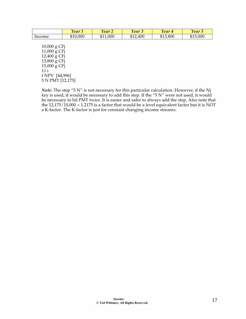
Year 1 Year 2 Year 3 Year 4 Year 5 Income $10,000 $11,000 $12,400 $13,800 $15,000
10,000 g CFj 11,000 g CFj 12,400 g CFj 13,800 g CFj 15,000 g CFj 11 i f NPV [44,996] 5 N PMT [12,175] Note: The step “5 N” is not necessary for this particular calculation. However, if the Nj key is used, it would be necessary to add this step. If the “5 N” were not used, it would be necessary to hit PMT twice. It is easier and safer to always add the step. Also note that the 12,175/10,000 = 1.2175 is a factor that would be a level equivalent factor but it is NOT a K-factor. The K-factor is just for constant changing income streams.
Income © Ted Whitmer, All Rights Reserved.
18"
Chapter 49 Direct Capitalization
Overview
Direct capitalization is the use of a multiplier or capitalization rate to process an income to value. In direct capitalization, the yield rate is not specified. Also, the change in income and value is not explicitly set forth. For residential valuation the formula is as follows… Monthly rent x GMRM = Value The GMRM is the gross monthly rent multiplier and is found by taking a sale price of a property that has sold and dividing it by the rent that it was achieving at the time of sale. An appraiser should be careful to assess if the
Income © Ted Whitmer, All Rights Reserved.
19"
Chapter 50 Direct Capitalization - Commercial
Overview
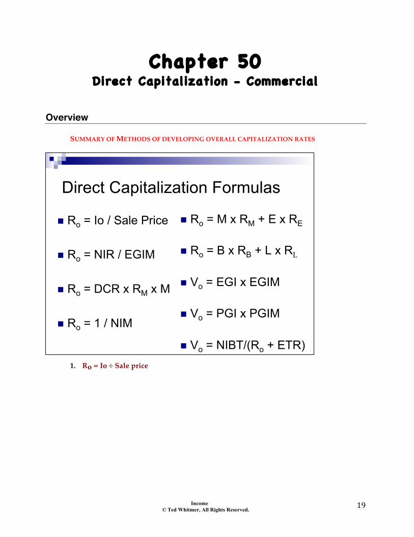
SUMMARY OF METHODS OF DEVELOPING OVERALL CAPITALIZATION RATES """"
1. Ro = Io ÷ Sale price
Direct Capitalization Formulas
! Ro = Io / Sale Price
! Ro = NIR / EGIM
! Ro = DCR x RM x M
! Ro = 1 / NIM
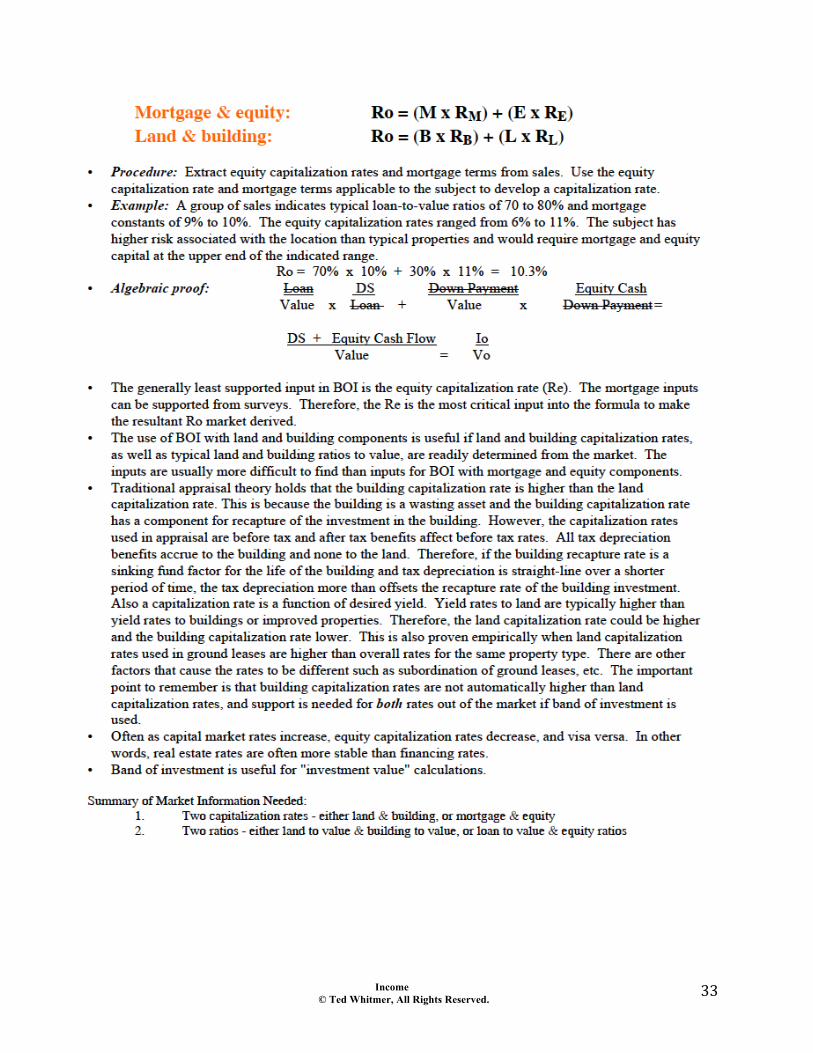
! Ro = M x RM + E x RE ! Ro = B x RB + L x RL
! Vo = EGI x EGIM
! Vo = PGI x PGIM
! Vo = NIBT/(Ro + ETR)
Income © Ted Whitmer, All Rights Reserved.
20"
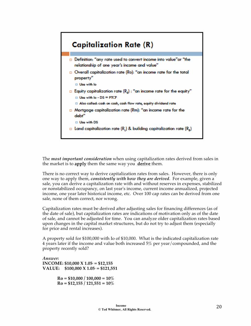
The most important consideration when using capitalization rates derived from sales in the market is to apply them the same way you derive them. There is no correct way to derive capitalization rates from sales. However, there is only one way to apply them, consistently with how they are derived. For example, given a sale, you can derive a capitalization rate with and without reserves in expenses, stabilized or nonstabilized occupancy, on last year's income, current income annualized, projected income, one year later historical income, etc. Over 100 cap rates can be derived from one sale, none of them correct, nor wrong. Capitalization rates must be derived after adjusting sales for financing differences (as of the date of sale), but capitalization rates are indications of motivation only as of the date of sale, and cannot be adjusted for time. You can analyze older capitalization rates based upon changes in the capital market structures, but do not try to adjust them (especially for price and rental increases). A property sold for $100,000 with Io of $10,000. What is the indicated capitalization rate 4 years later if the income and value both increased 5% per year/compounded, and the property recently sold? Answer: INCOME: $10,000 X 1.054 = $12,155 VALUE: $100,000 X 1.054 = $121,551 Ro = $10,000 / 100,000 = 10% Ro = $12,155 / 121,551 = 10%
Income © Ted Whitmer, All Rights Reserved.
21"
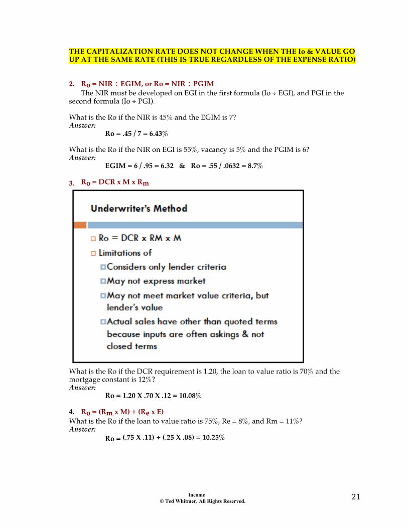
THE CAPITALIZATION RATE DOES NOT CHANGE WHEN THE Io & VALUE GO UP AT THE SAME RATE (THIS IS TRUE REGARDLESS OF THE EXPENSE RATIO) 2. Ro = NIR ÷ EGIM, or Ro = NIR ÷ PGIM The NIR must be developed on EGI in the first formula (Io ÷ EGI), and PGI in the second formula (Io ÷ PGI). What is the Ro if the NIR is 45% and the EGIM is 7? Answer: Ro = .45 / 7 = 6.43% What is the Ro if the NIR on EGI is 55%, vacancy is 5% and the PGIM is 6? Answer: EGIM = 6 / .95 = 6.32 & Ro = .55 / .0632 = 8.7% 3. Ro = DCR x M x Rm
What is the Ro if the DCR requirement is 1.20, the loan to value ratio is 70% and the mortgage constant is 12%? Answer: Ro = 1.20 X .70 X .12 = 10.08% 4. Ro = (Rm x M) + (Re x E) What is the Ro if the loan to value ratio is 75%, Re = 8%, and Rm = 11%? Answer: Ro = (.75 X .11) + (.25 X .08) = 10.25%
Income © Ted Whitmer, All Rights Reserved.
22"
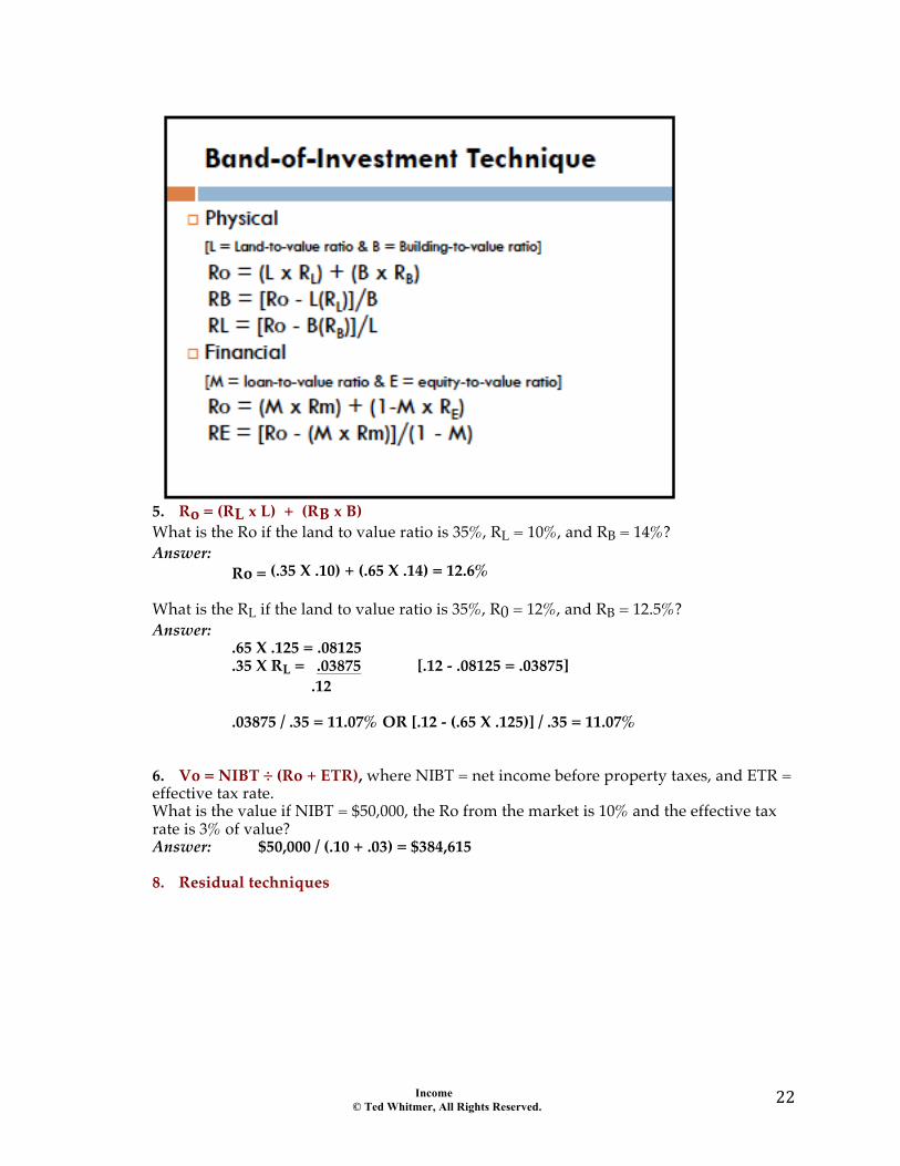
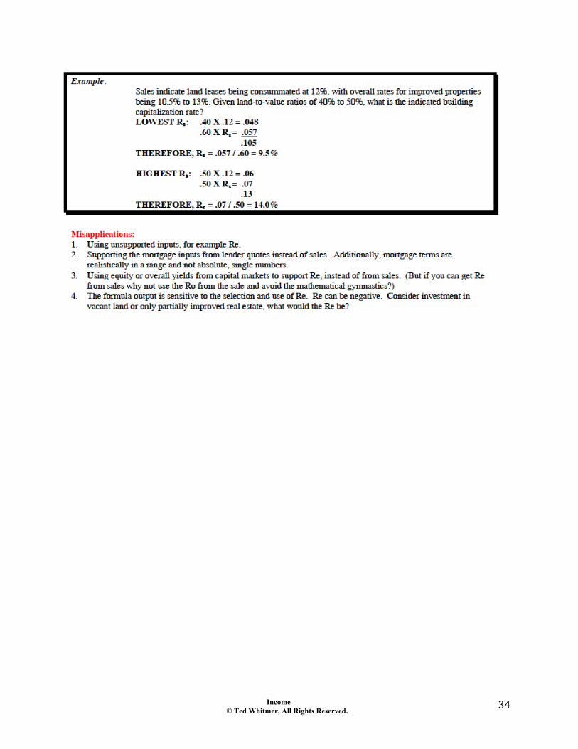
5. Ro = (RL x L) + (RB x B) What is the Ro if the land to value ratio is 35%, RL = 10%, and RB = 14%? Answer: Ro = (.35 X .10) + (.65 X .14) = 12.6% What is the RL if the land to value ratio is 35%, R0 = 12%, and RB = 12.5%? Answer: .65 X .125 = .08125 .35 X RL = .03875 [.12 - .08125 = .03875] .12 .03875 / .35 = 11.07% OR [.12 - (.65 X .125)] / .35 = 11.07% 6. Vo = NIBT ÷ (Ro + ETR), where NIBT = net income before property taxes, and ETR = effective tax rate. What is the value if NIBT = $50,000, the Ro from the market is 10% and the effective tax rate is 3% of value? Answer: $50,000 / (.10 + .03) = $384,615 8. Residual techniques
Income © Ted Whitmer, All Rights Reserved.
23"
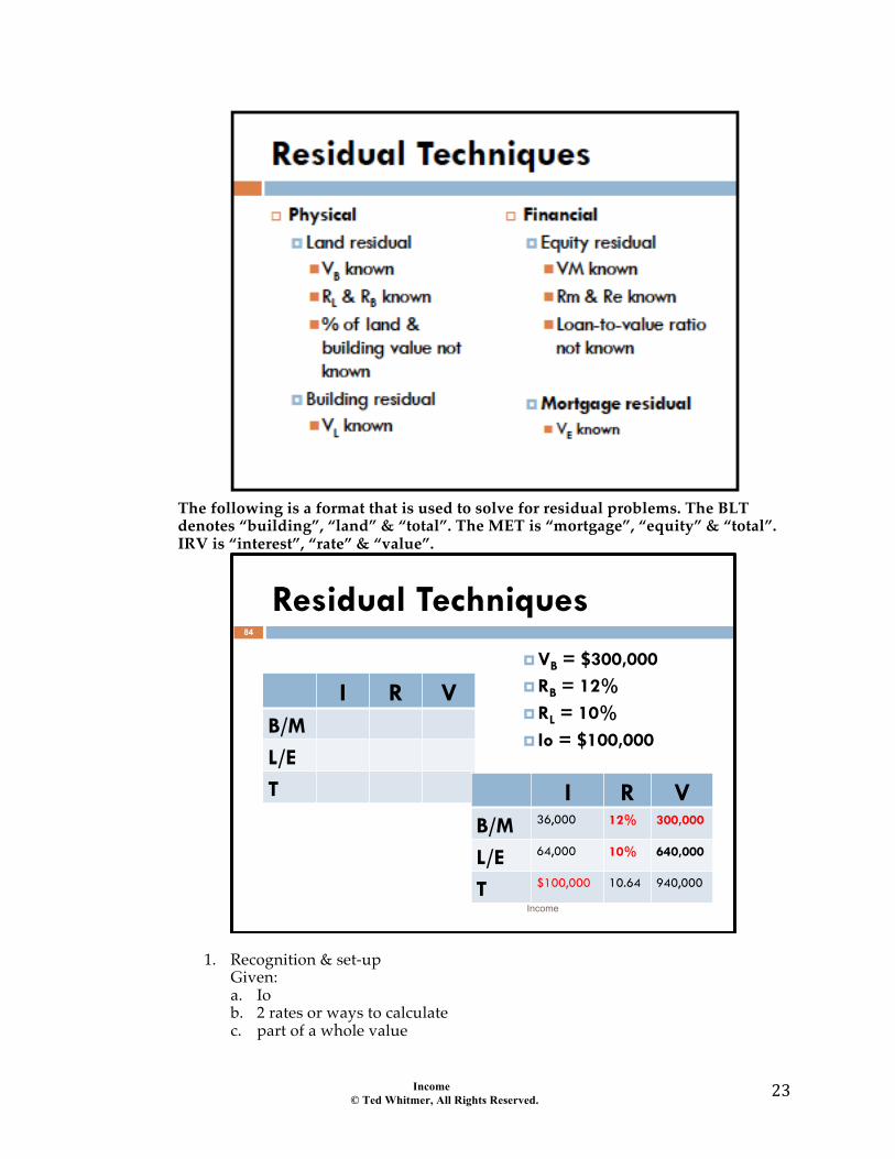
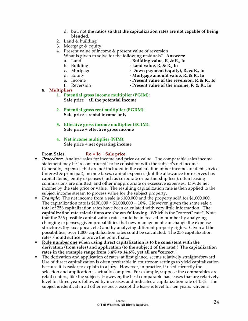
The following is a format that is used to solve for residual problems. The BLT denotes “building”, “land” & “total”. The MET is “mortgage”, “equity” & “total”. IRV is “interest”, “rate” & “value”.
1. Recognition & set-up Given: a. Io b. 2 rates or ways to calculate c. part of a whole value
Residual Techniques
I R V B/M L/E T
! VB = $300,000 ! RB = 12% ! RL = 10% ! Io = $100,000
I R V B/M 36,000 12% 300,000
L/E 64,000 10% 640,000
T $100,000 10.64 940,000
84
Income
Income © Ted Whitmer, All Rights Reserved.
24"
d. but, not the ratios so that the capitalization rates are not capable of being blended.
2. Land & building 3. Mortgage & equity 4. Present value of income & present value of reversion What is given to solve for the following residuals? Answers: a. Land - Building value, RL & RB, Io b. Building - Land value, RL & RB, Io c. Mortgage - Down payment (equity), RM & RE, Io d. Equity - Mortgage amount value, RM & RE, Io e. Income - Present value of the reversion, RI & RN, Io f. Reversion - Present value of the income, RI & RN, Io 8. Multipliers 1. Potential gross income multiplier (PGIM): Sale price ÷ all the potential income 2. Potential gross rent multiplier (PGRM): Sale price ÷ rental income only 3. Effective gross income multiplier (EGIM): Sale price ÷ effective gross income 4. Net income multiplier (NIM): Sale price ÷ net operating income From Sales Ro = Io ÷ Sale price
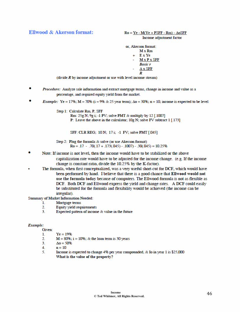
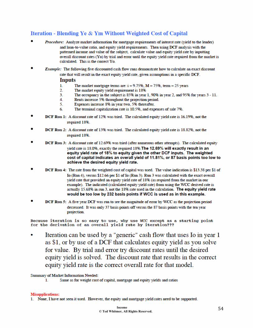
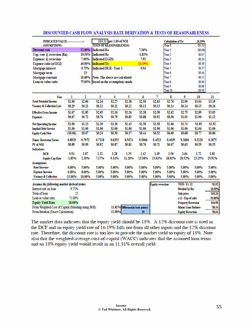
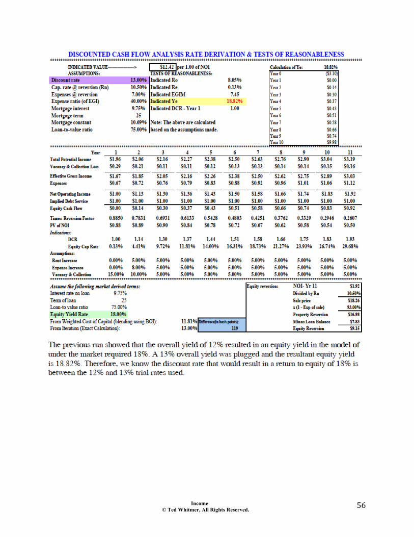
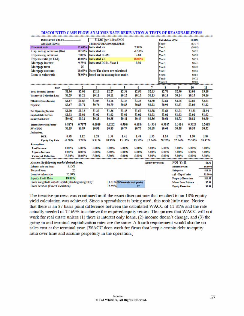
• Procedure: Analyze sales for income and price or value. The comparable sales income statement may be "reconstructed" to be consistent with the subject's net income. Generally, expenses that are not included in the calculation of net income are debt service (interest & principal), income taxes, capital expenses (but the allowance for reserves has capital items), entity expenses (such as corporate or partnership fees), often leasing commissions are omitted, and other inappropriate or excessive expenses. Divide net income by the sale price or value. The resulting capitalization rate is then applied to the subject income stream to process value for the subject property.
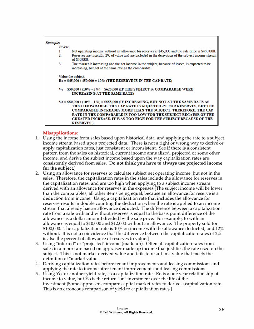
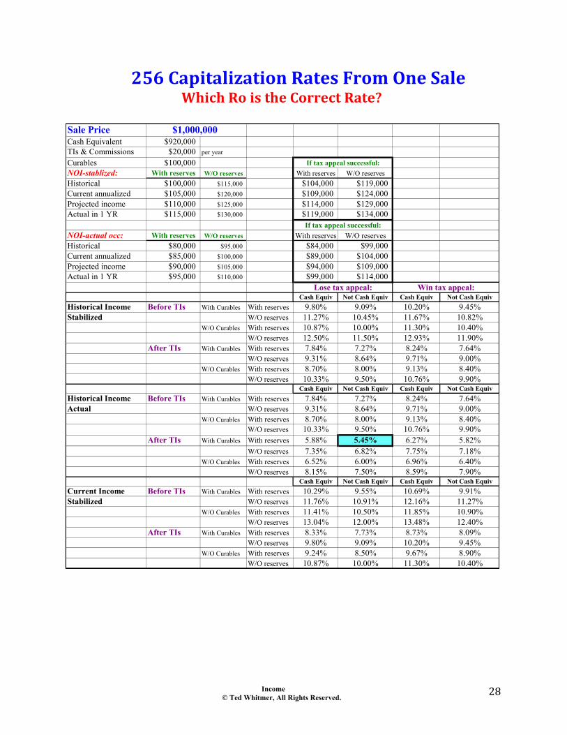
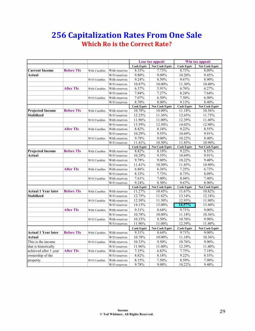
• Example: The net income from a sale is $100,000 and the property sold for $1,000,000. The capitalization rate is $100,000 ÷ $1,000,000 = 10%. However, given the same sale a total of 256 capitalization rates have been calculated with very little information. The capitalization rate calculations are shown following. Which is the "correct" rate? Note that the 256 possible capitalization rates could be increased in number by analyzing changing expenses, given probabilities that new management can change the expense structures (by tax appeal, etc.) and by analyzing different property rights. Given all the possibilities, over 1,000 capitalization rates could be calculated. The 256 capitalization rates should suffice to prove the point that...
• Rule number one when using direct capitalization is to be consistent with the derivation (from sales) and application (to the subject) of the rate!!! The capitalization rates in the example range from 5.4% to 14.6%, yet all are "correct."
• The derivation and application of rates, at first glance, seems relatively straight-forward. Use of direct capitalization is often preferable in courtroom settings to yield capitalization because it is easier to explain to a jury. However, in practice, if used correctly the selection and application is actually complex. For example, suppose the comparables are retail centers, like the subject. However, the best comparable has leases that are relatively level for three years followed by increases and indicates a capitalization rate of 13%. The subject is identical in all other respects except the lease is level for ten years. Given a

Income © Ted Whitmer, All Rights Reserved.
25"
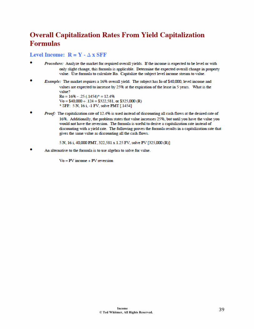
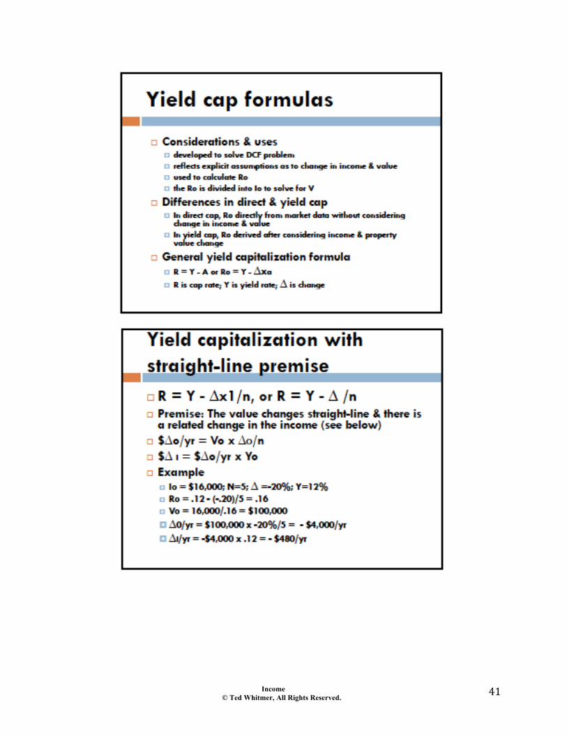
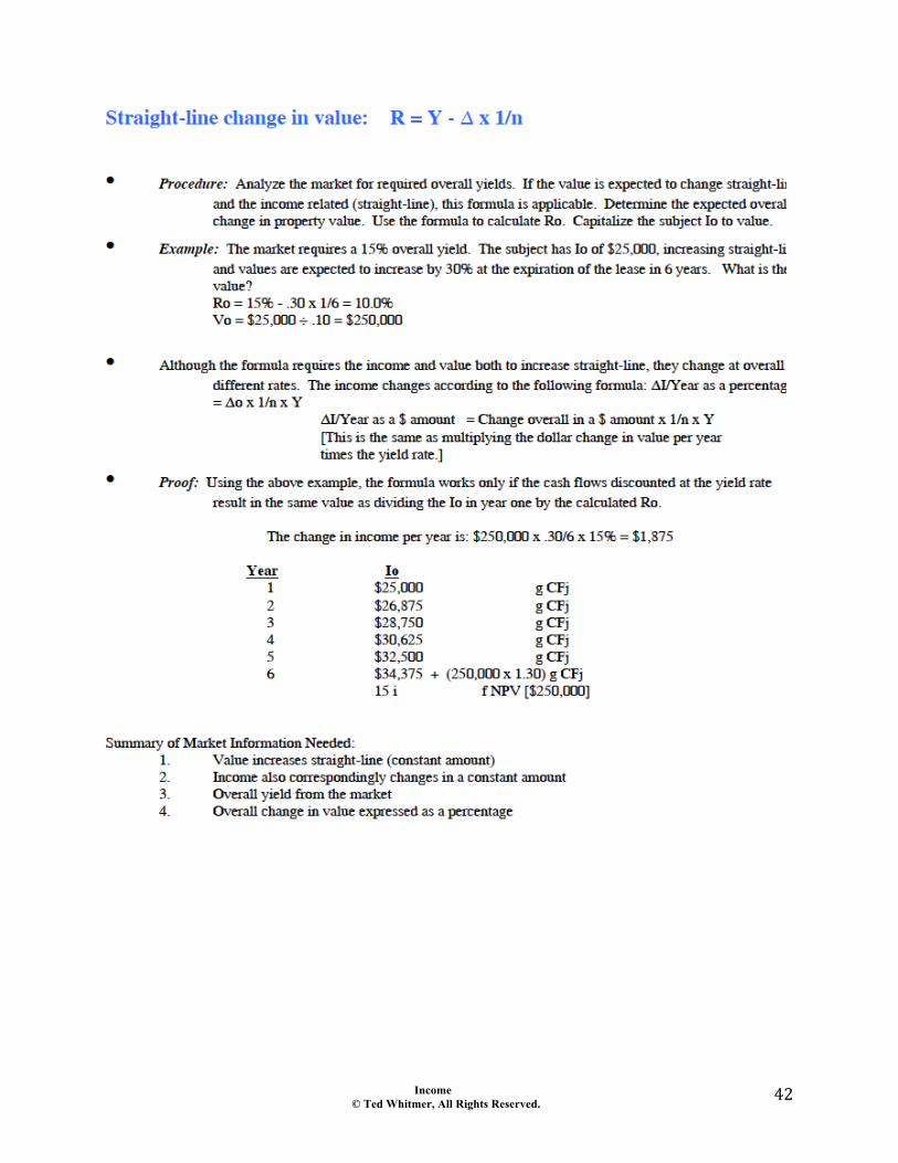
rising market the capitalization rate should be greater for the subject than 13%, and less than 13% if a declining market. The longer the income is expected to be level over a holding period, the closer the capitalization rate is to the yield rate. The yield rate is the rate of return over the entire period of ownership, while the capitalization rate is only an expression of a one year return. The relationship in a very simple model (we will look at later) is R = Y - ∆o x SFF, where ∆o is the overall change in value, and the model assumes income will remain level over the holding period. Given a long expected level income ∆o x SFF becomes smaller and the R is approximately equal to Y. In nontechnical terms the capitalization rate is near the yield rate when expected income and value change is small. The more the value and income are expected to change, the larger the spread between the capitalization and yield rate.
• Multipliers such as effective gross income and potential gross income multipliers are also application of direct capitalization. In fact, the overall capitalization rate is the reciprocal of a net income multiplier, and an effective gross income multiplier is the net income multiplier times the net income ratio (which is 1 minus the operating expense ratio). We will also later look at this relationship expressed in the formula: R = NIR ÷ EGIM. There is obviously a relationship between the EGIM, Ro, OER, and Yo.
• The Ro should be consistent with the risk in a property, the higher the risk relative to other sales, generally the higher the capitalization rate.
Summary of Market Information Needed:
1. Net operating income = Potential gross income - vacancy & collection loss - operating expenses
2. Sale price or adjusted sale price (adjusted for cash equivalency, personal property or business value included, property rights, etc.)
Income © Ted Whitmer, All Rights Reserved.
26"
Misapplications:
1. Using the income from sales based upon historical data, and applying the rate to a subject income stream based upon projected data. [There is not a right or wrong way to derive or apply capitalization rates, just consistent or inconsistent. See if there is a consistent pattern from the sales on historical, current income annualized, projected or some other income, and derive the subject income based upon the way capitalization rates are consistently derived from sales. Do not think you have to always use projected income for the subject.]
2. Using an allowance for reserves to calculate subject net operating income, but not in the sales. Therefore, the capitalization rates in the sales include the allowance for reserves in the capitalization rates, and are too high when applying to a subject income stream derived with an allowance for reserves in the expenses.[The subject income will be lower than the comparables, all other items being equal, because an allowance for reserve is a deduction from income. Using a capitalization rate that includes the allowance for reserves results in double counting the deduction when the rate is applied to an income stream that already has an allowance deducted. The difference between a capitalization rate from a sale with and without reserves is equal to the basis point difference of the allowance as a dollar amount divided by the sale price. For example, Io with an allowance is equal to $10,000 and $12,000 without an allowance. The property sold for $100,000. The capitalization rate is 10% on income with the allowance deducted, and 12% without. It is not a coincidence that the difference between the capitalization rates of 2% is also the percent of allowance of reserves to value.]
3. Using "inferred" or "projected" income (made up). Often all capitalization rates from sales in a report are based on appraiser made up income that justifies the rate used on the subject. This is not market derived value and fails to result in a value that meets the definition of "market value."
4. Deriving capitalization rates before tenant improvements and leasing commissions and applying the rate to income after tenant improvements and leasing commissions.
5. Using Yo, or another yield rate, as a capitalization rate. Ro is a one year relationship of income to value, but Yo is the return "on" investment over the life of the investment.[Some appraisers compare capital market rates to derive a capitalization rate. This is an erroneous comparison of yield to capitalization rates.]
Income © Ted Whitmer, All Rights Reserved.
27"
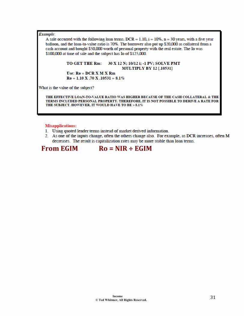
IMPORTANT: All other methods in direct capitalization (such as band of investment & DCR analysis to derive Ro) are not generally preferred methods to primarily derive capitalization rates. If you have the inputs needed to derive the capitalization rate, you already have income divided by value, and do not need the alternative formulas. The alternative equations are useful (1) to adjust market-derived rates to better apply to the subject and (2) for tests of reasonableness. Furthermore, they are useful for adjusting previously market derived capitalization rates when time has lapsed since the derivation of the rates from sales, and subsequently no or little sales information is available. The following are 256 capitalization rates from one, the same sale. The rates range from 5.4% to 14.6%, depending upon which income and which price or value was used. Therefore, the income and price or value used to develop the Ro must be consistent with the income developed for the subject and the value or price that is being measured.
Income © Ted Whitmer, All Rights Reserved.
28"
256$Capitalization$Rates$From$One$Sale$Which$Ro$is$the$Correct$Rate?$
$Sale PriceCash Equivalent $920,000TIs & Commissions $20,000 per year
Curables $100,000NOI-stablized: With reserves W/O reserves With reserves W/O reservesHistorical $100,000 $115,000 $104,000 $119,000Current annualized $105,000 $120,000 $109,000 $124,000Projected income $110,000 $125,000 $114,000 $129,000Actual in 1 YR $115,000 $130,000 $119,000 $134,000
NOI-actual occ: With reserves W/O reserves With reserves W/O reservesHistorical $80,000 $95,000 $84,000 $99,000Current annualized $85,000 $100,000 $89,000 $104,000Projected income $90,000 $105,000 $94,000 $109,000Actual in 1 YR $95,000 $110,000 $99,000 $114,000
Cash Equiv Not Cash Equiv Cash Equiv Not Cash EquivHistorical Income Before TIs With Curables With reserves 9.80% 9.09% 10.20% 9.45%Stabilized W/O reserves 11.27% 10.45% 11.67% 10.82%
W/O Curables With reserves 10.87% 10.00% 11.30% 10.40%W/O reserves 12.50% 11.50% 12.93% 11.90%
After TIs With Curables With reserves 7.84% 7.27% 8.24% 7.64%W/O reserves 9.31% 8.64% 9.71% 9.00%
W/O Curables With reserves 8.70% 8.00% 9.13% 8.40%W/O reserves 10.33% 9.50% 10.76% 9.90%
Cash Equiv Not Cash Equiv Cash Equiv Not Cash EquivHistorical Income Before TIs With Curables With reserves 7.84% 7.27% 8.24% 7.64%Actual W/O reserves 9.31% 8.64% 9.71% 9.00%
W/O Curables With reserves 8.70% 8.00% 9.13% 8.40%W/O reserves 10.33% 9.50% 10.76% 9.90%
After TIs With Curables With reserves 5.88% 5.45% 6.27% 5.82%W/O reserves 7.35% 6.82% 7.75% 7.18%
W/O Curables With reserves 6.52% 6.00% 6.96% 6.40%W/O reserves 8.15% 7.50% 8.59% 7.90%
Cash Equiv Not Cash Equiv Cash Equiv Not Cash EquivCurrent Income Before TIs With Curables With reserves 10.29% 9.55% 10.69% 9.91%Stabilized W/O reserves 11.76% 10.91% 12.16% 11.27%
W/O Curables With reserves 11.41% 10.50% 11.85% 10.90%W/O reserves 13.04% 12.00% 13.48% 12.40%
After TIs With Curables With reserves 8.33% 7.73% 8.73% 8.09%W/O reserves 9.80% 9.09% 10.20% 9.45%
W/O Curables With reserves 9.24% 8.50% 9.67% 8.90%W/O reserves 10.87% 10.00% 11.30% 10.40%
$1,000,000
Lose tax appeal: Win tax appeal:
If tax appeal successful:
If tax appeal successful:
Income © Ted Whitmer, All Rights Reserved.
29"
256$Capitalization$Rates$From$One$Sale$Which$Ro$is$the$Correct$Rate?$
$
$Cash Equiv Not Cash Equiv Cash Equiv Not Cash Equiv
Current Income Before TIs With Curables With reserves 8.33% 7.73% 8.73% 8.09%Actual W/O reserves 9.80% 9.09% 10.20% 9.45%
W/O Curables With reserves 9.24% 8.50% 9.67% 8.90%W/O reserves 10.87% 10.00% 11.30% 10.40%
After TIs With Curables With reserves 6.37% 5.91% 6.76% 6.27%W/O reserves 7.84% 7.27% 8.24% 7.64%
W/O Curables With reserves 7.07% 6.50% 7.50% 6.90%W/O reserves 8.70% 8.00% 9.13% 8.40%
Cash Equiv Not Cash Equiv Cash Equiv Not Cash EquivProjected Income Before TIs With Curables With reserves 10.78% 10.00% 11.18% 10.36%Stabilized W/O reserves 12.25% 11.36% 12.65% 11.73%
W/O Curables With reserves 11.96% 11.00% 12.39% 11.40%W/O reserves 13.59% 12.50% 14.02% 12.90%
After TIs With Curables With reserves 8.82% 8.18% 9.22% 8.55%W/O reserves 10.29% 9.55% 10.69% 9.91%
W/O Curables With reserves 9.78% 9.00% 10.22% 9.40%W/O reserves 11.41% 10.50% 11.85% 10.90%
Cash Equiv Not Cash Equiv Cash Equiv Not Cash EquivProjected Income Before TIs With Curables With reserves 8.82% 8.18% 9.22% 8.55%Actual W/O reserves 10.29% 9.55% 10.69% 9.91%
W/O Curables With reserves 9.78% 9.00% 10.22% 9.40%W/O reserves 11.41% 10.50% 11.85% 10.90%
After TIs With Curables With reserves 6.86% 6.36% 7.25% 6.73%W/O reserves 8.33% 7.73% 8.73% 8.09%
W/O Curables With reserves 7.61% 7.00% 8.04% 7.40%W/O reserves 9.24% 8.50% 9.67% 8.90%
Cash Equiv Not Cash Equiv Cash Equiv Not Cash EquivActual 1 Year later Before TIs With Curables With reserves 11.27% 10.45% 11.67% 10.82%Stabilized W/O reserves 12.75% 11.82% 13.14% 12.18%
W/O Curables With reserves 12.50% 11.50% 12.93% 11.90%W/O reserves 14.13% 13.00% 14.57% 13.40%
After TIs With Curables With reserves 9.31% 8.64% 9.71% 9.00%W/O reserves 10.78% 10.00% 11.18% 10.36%
W/O Curables With reserves 10.33% 9.50% 10.76% 9.90%W/O reserves 11.96% 11.00% 12.39% 11.40%
Cash Equiv Not Cash Equiv Cash Equiv Not Cash EquivActual 1 Year later Before TIs With Curables With reserves 9.31% 8.64% 9.71% 9.00%Actual W/O reserves 10.78% 10.00% 11.18% 10.36%This is the income W/O Curables With reserves 10.33% 9.50% 10.76% 9.90%that is historically W/O reserves 11.96% 11.00% 12.39% 11.40%achieved after 1 year After TIs With Curables With reserves 7.35% 6.82% 7.75% 7.18%ownership of the W/O reserves 8.82% 8.18% 9.22% 8.55%property. W/O Curables With reserves 8.15% 7.50% 8.59% 7.90%
W/O reserves 9.78% 9.00% 10.22% 9.40%
Lose tax appeal: Win tax appeal:

Income © Ted Whitmer, All Rights Reserved.
30"
From$DCR$ $ Ro$=$DCR$x$Rm$x$M$
"
Income © Ted Whitmer, All Rights Reserved.
31"
"
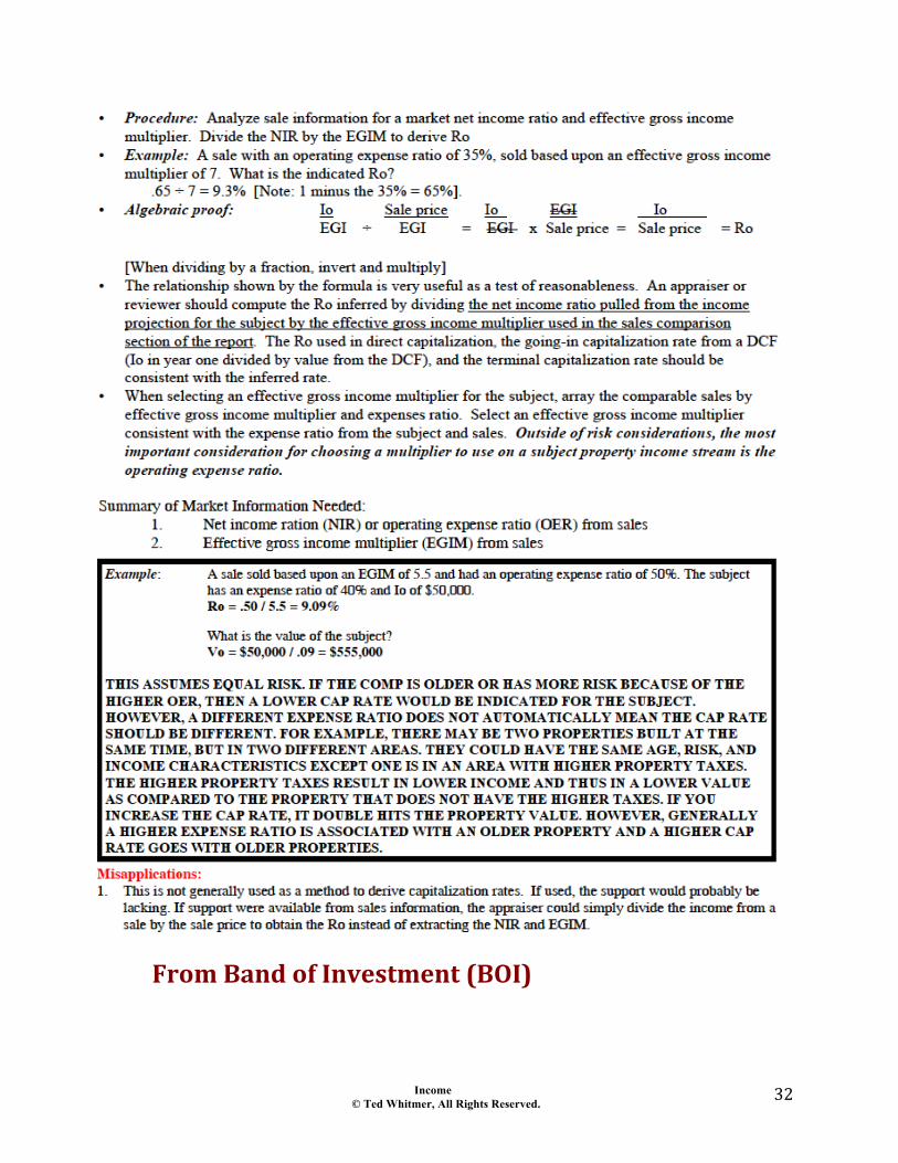
"$ $ From$EGIM$ $ Ro$=$NIR$÷$EGIM"
Income © Ted Whitmer, All Rights Reserved.
32"
"
"
""$ From$Band$of$Investment$(BOI)$$ $
$ "
Income © Ted Whitmer, All Rights Reserved.
33"
Income © Ted Whitmer, All Rights Reserved.
34"
""
Income © Ted Whitmer, All Rights Reserved.
35"
Chapter 51 Yield Capitalization
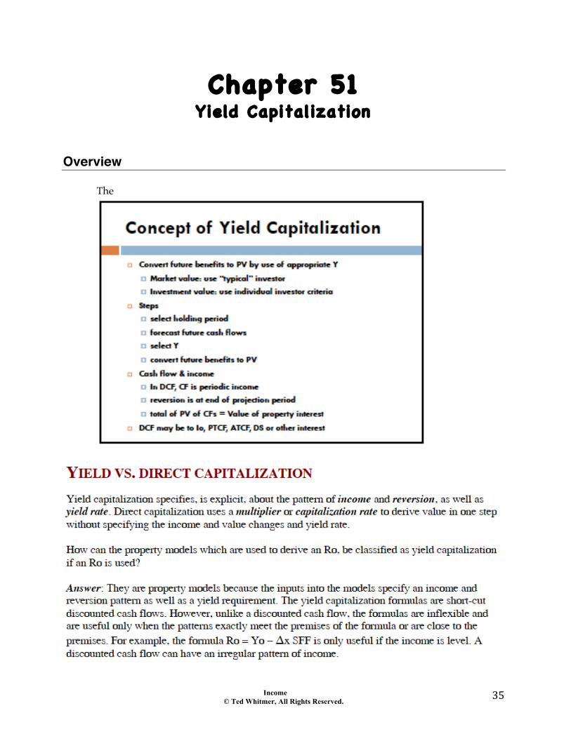
Overview
The
""
Income © Ted Whitmer, All Rights Reserved.
36"
"""$
Income$Models""
"
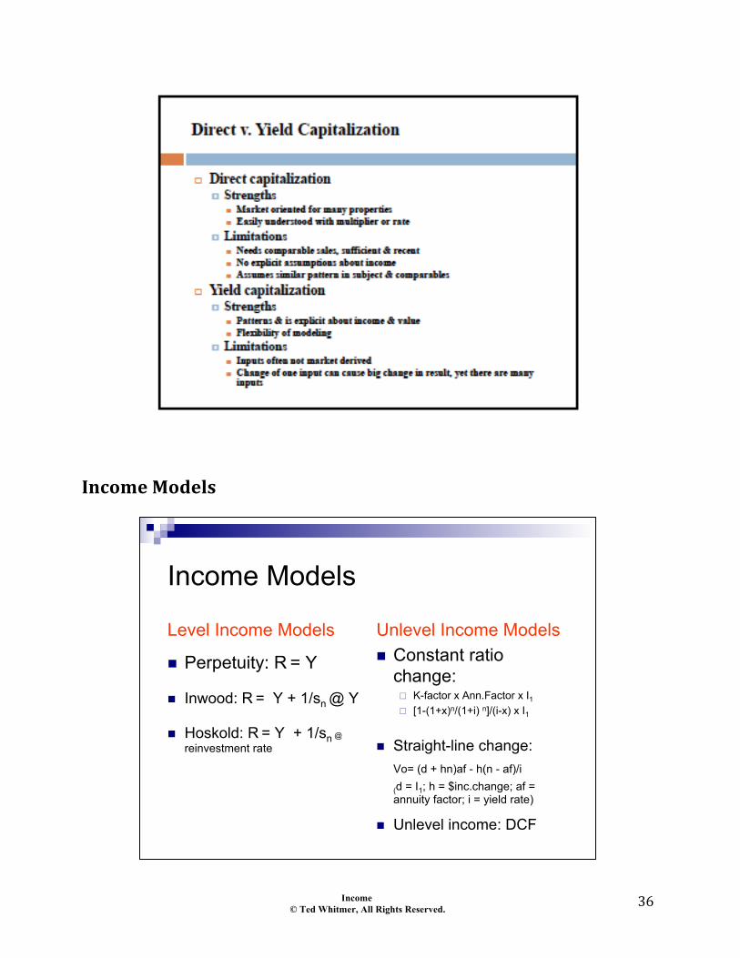
Income Models
Level Income Models
! Perpetuity: R = Y
! Inwood: R = Y + 1/sn @ Y
! Hoskold: R = Y + 1/sn @
reinvestment rate
Unlevel Income Models ! Constant ratio
change: " K-factor x Ann.Factor x I1
" [1-(1+x)n/(1+i) n]/(i-x) x I1
! Straight-line change: Vo= (d + hn)af - h(n - af)/i (d = I1; h = $inc.change; af = annuity factor; i = yield rate)
! Unlevel income: DCF
Income © Ted Whitmer, All Rights Reserved.
37"
"Property$Models$
""
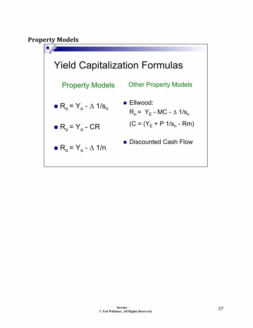
Yield Capitalization Formulas
Property Models
! Ro = Yo - ∆ 1/sn
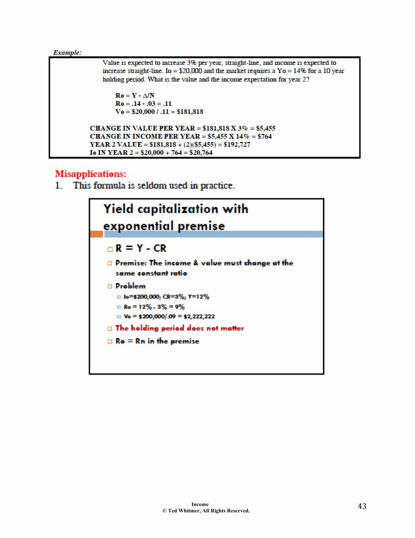
! Ro = Yo - CR
! Ro = Yo - ∆ 1/n
Other Property Models
! Ellwood: Ro = YE - MC - ∆ 1/sn
(C = (YE + P 1/sn - Rm) ! Discounted Cash Flow

Income © Ted Whitmer, All Rights Reserved.
38"
""
"
Investment Model Decision Tree Combining Income & Property Models If the income is level: Use R = Y - ∆1/sn
! If only income or no value in
reversion, then Δ = -1 (This means you will add the 1/sn to Y)
! If reinvestment is at a different rate than Y, then calculate the 1/sn @ lower rate (Hoskold premise)
! If the income is in perpetuity or there is no change in value then Δ = 0
! Otherwise, compute the 1/sn @ Y (Inwood premise)
! If the income is unlevel, calculate equivalent level income & use the above formula
If the income is unlevel: " & straight-line change in value
with related change in income
! R = Y - ∆ 1/n " & constant ratio change in income
& value ! R = Y - CR
" & given Ye & mortgage terms (Ellwood)
! R = Y - MC - ∆ 1/sn " otherwise, use a DCF
Income © Ted Whitmer, All Rights Reserved.
39"
Income © Ted Whitmer, All Rights Reserved.
40"
Income © Ted Whitmer, All Rights Reserved.
41"
Income © Ted Whitmer, All Rights Reserved.
42"
Income © Ted Whitmer, All Rights Reserved.
43"
Income © Ted Whitmer, All Rights Reserved.
44"
Income © Ted Whitmer, All Rights Reserved.
45"
Income © Ted Whitmer, All Rights Reserved.
46"
Income © Ted Whitmer, All Rights Reserved.
47"
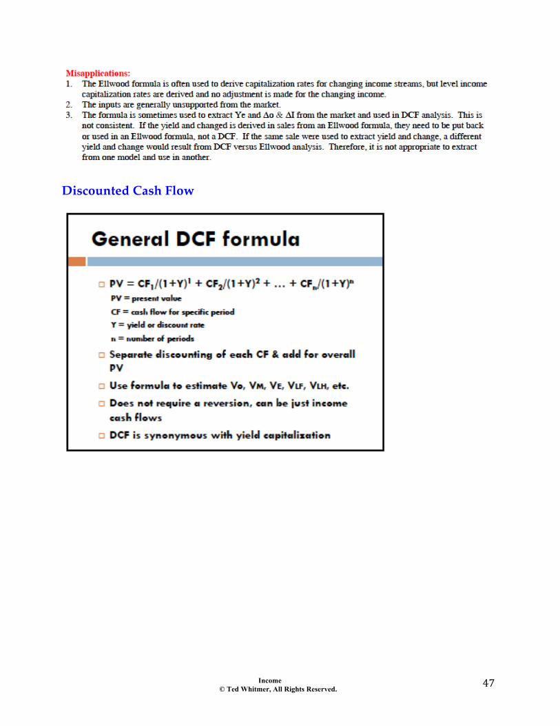
Discounted Cash Flow
Income © Ted Whitmer, All Rights Reserved.
48"
Income © Ted Whitmer, All Rights Reserved.
49"
Income © Ted Whitmer, All Rights Reserved.
50"
Chapter 52 Leverage
Overview
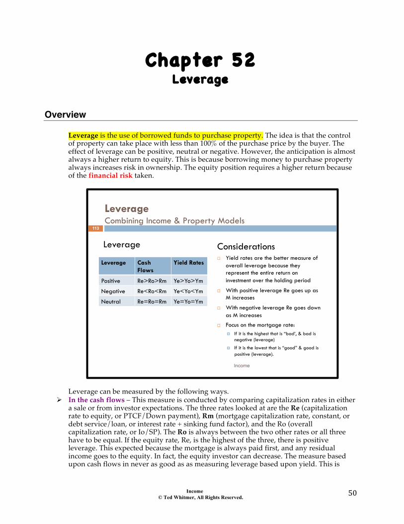
Leverage is the use of borrowed funds to purchase property. The idea is that the control of property can take place with less than 100% of the purchase price by the buyer. The effect of leverage can be positive, neutral or negative. However, the anticipation is almost always a higher return to equity. This is because borrowing money to purchase property always increases risk in ownership. The equity position requires a higher return because of the financial risk taken.
Leverage can be measured by the following ways.
# In the cash flows – This measure is conducted by comparing capitalization rates in either a sale or from investor expectations. The three rates looked at are the Re (capitalization rate to equity, or PTCF/Down payment), Rm (mortgage capitalization rate, constant, or debt service/loan, or interest rate + sinking fund factor), and the Ro (overall capitalization rate, or Io/SP). The Ro is always between the two other rates or all three have to be equal. If the equity rate, Re, is the highest of the three, there is positive leverage. This expected because the mortgage is always paid first, and any residual income goes to the equity. In fact, the equity investor can decrease. The measure based upon cash flows in never as good as as measuring leverage based upon yield. This is
Leverage Combining Income & Property Models Leverage
Considerations ! Yield rates are the better measure of
overall leverage because they represent the entire return on investment over the holding period
! With positive leverage Re goes up as M increases
! With negative leverage Re goes down as M increases
! Focus on the mortgage rate: ! If it is the highest that is “bad’, & bad is
negative (leverage)
! If it is the lowest that is “good” & good is positive (leverage).
113
Leverage Cash Flows
Yield Rates
Positive Re>Ro>Rm Ye>Yo>Ym
Negative Re<Ro<Rm Ye<Yo<Ym
Neutral Re=Ro=Rm Ye=Yo=Ym
Income
Income © Ted Whitmer, All Rights Reserved.
51"
because the yield rates include the first year returns, but the capitalization rates are just the first year return in an investment. Loosely put, the yield rates are a time weighted average of all capitalization rates, including the first year. Note also that if all rates are equal, there is still leverage, there is just no affect of the leverage. Note further, that if all rates are equal, the mortgage holder is in a favorable position relative to equity because the equity position is always with higher risk.
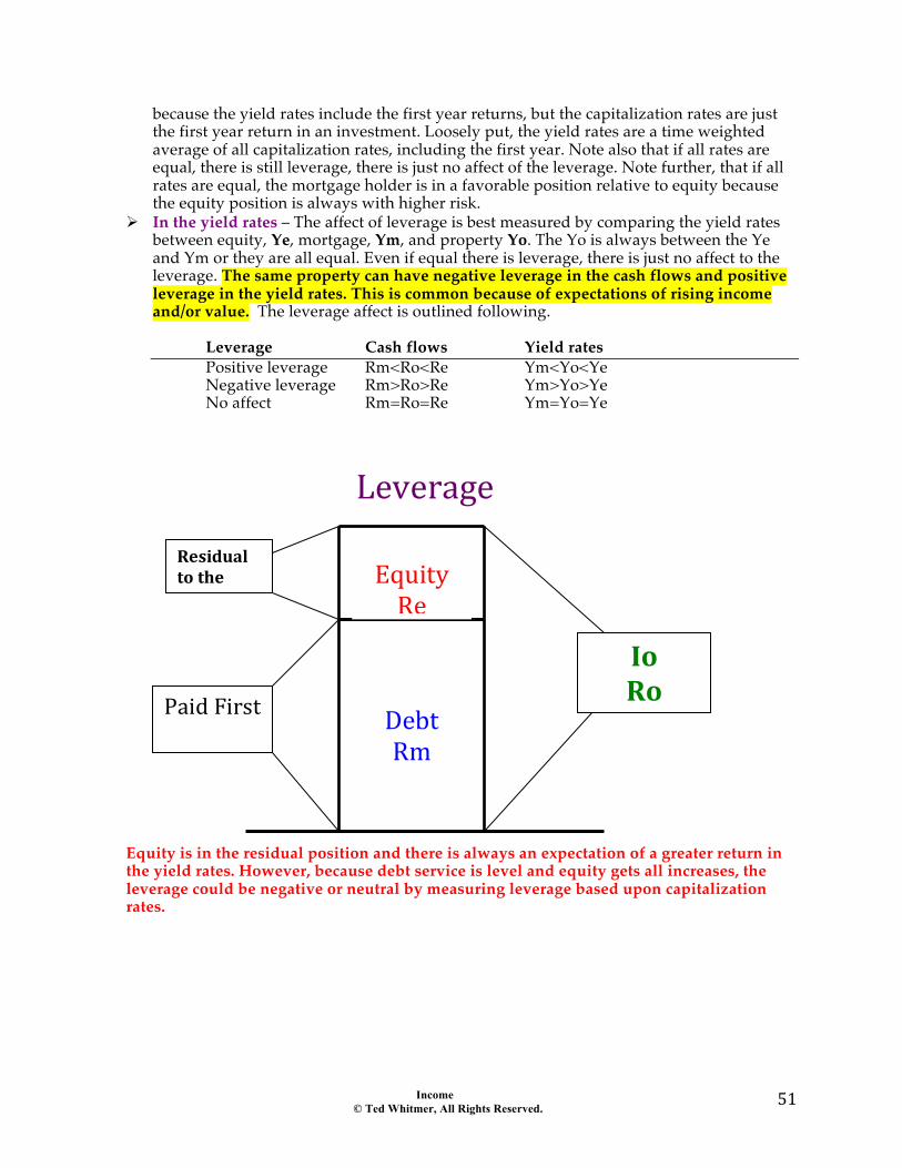
# In the yield rates – The affect of leverage is best measured by comparing the yield rates between equity, Ye, mortgage, Ym, and property Yo. The Yo is always between the Ye and Ym or they are all equal. Even if equal there is leverage, there is just no affect to the leverage. The same property can have negative leverage in the cash flows and positive leverage in the yield rates. This is common because of expectations of rising income and/or value. The leverage affect is outlined following. Leverage Cash flows Yield rates Positive leverage Rm<Ro<Re Ym<Yo<Ye Negative leverage Rm>Ro>Re Ym>Yo>Ye No affect Rm=Ro=Re Ym=Yo=Ye
"
"Equity is in the residual position and there is always an expectation of a greater return in the yield rates. However, because debt service is level and equity gets all increases, the leverage could be negative or neutral by measuring leverage based upon capitalization rates. $
Equity"Re"
Debt"Rm"
Io$Ro$Paid"First"
Residual$to$the$Debt$$
Leverage"
Income © Ted Whitmer, All Rights Reserved.
52"
Chapter 53 Weighted Average Cost of Capital
Overview
The
Income © Ted Whitmer, All Rights Reserved.
53"
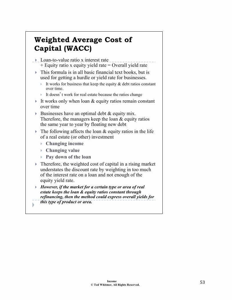
Weighted Average Cost of Capital (WACC) ! Loan-to-value ratio x interest rate
+ Equity ratio x equity yield rate = Overall yield rate ! This formula is in all basic financial text books, but is
used for getting a hurdle or yield rate for businesses. ! It works for business that keep the equity & debt ratios constant
over time. ! It doesn�t work for real estate because the ratios change
! It works only when loan & equity ratios remain constant over time
! Businesses have an optimal debt & equity mix. Therefore, the managers keep the loan & equity ratios the same year to year by floating new debt
! The following affects the loan & equity ratios in the life of a real estate (or other) investment ! Changing income ! Changing value ! Pay down of the loan
! Therefore, the weighted cost of capital in a rising market understates the discount rate by weighting in too much of the interest rate on a loan and not enough of the equity yield rate.
! However, if the market for a certain type or area of real estate keeps the loan & equity ratios constant through refinancing, then the method could express overall yields for this type of product or area.
Income © Ted Whitmer, All Rights Reserved.
54"
Income © Ted Whitmer, All Rights Reserved.
55"
Income © Ted Whitmer, All Rights Reserved.
56"
Income © Ted Whitmer, All Rights Reserved.
57"
Income © Ted Whitmer, All Rights Reserved.
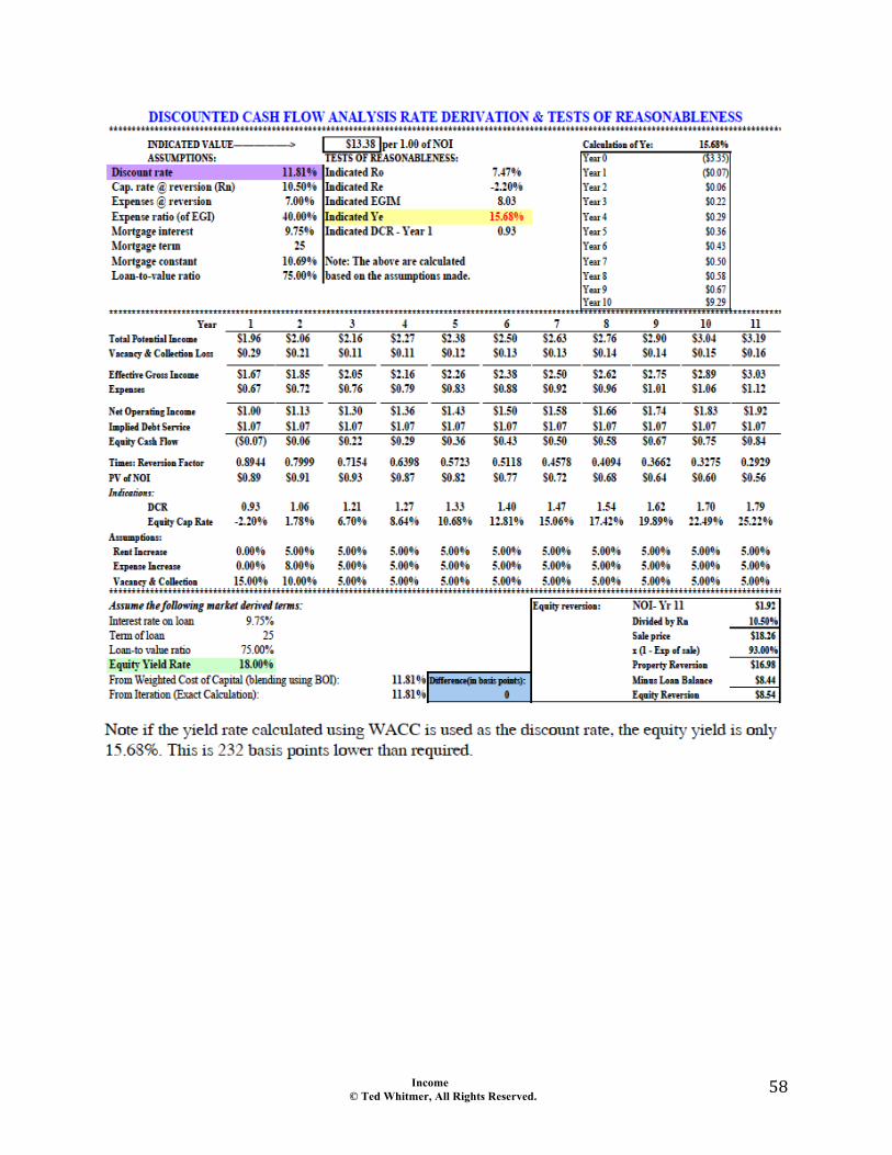
58"
Income © Ted Whitmer, All Rights Reserved.
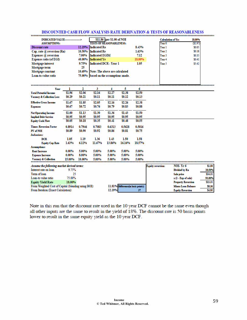
59"
Income © Ted Whitmer, All Rights Reserved.
60"
Chapter 54 Relationship of Rates
Overview
Capitalization rates 1. Ro
# Older properties often have higher Ro's because the investment in the building must be captured over a shorter period of time, and because of risk.
# If capital market rates rise, the Ro may rise because investment in real estate competes with other investments. However, if the capital market rates rise because of new tax laws or because of perceived inflation, the Ro could stay the same or decrease because of favorable tax treatment or because it may be looked at as an inflation hedge.
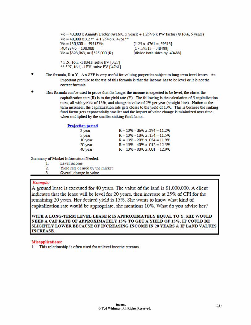
# A property subject to a long-term level lease generally has a higher Ro, than a similar property with shorter term leases because Ro = Yo - ∆xSFF. The ∆o x SFF becomes small when out in time, and this is the correct formula when income is level. (e.g. Yo=13%, ∆=25%, and n=15 with a level lease; Ro = .13 - (.25 x .0247*) = .124; therefore, there is only a 60 basis point difference). *Note: 15 N, 13 i, -1 FV, solve PMT [.0247] SFF.
# When looking at short-term return, focus on capitalization rankings over yield rate rankings.
# When analyzing Ro from sales: 1). Ro from a sale developed with no allowance for reserves is higher than an Ro where an allowance is included in expenses. 2). In a rising market, an Ro on historical income is lower than an Ro developed on expected income, and higher when income is expected to decline. 3). When Ro > Re, incomes and/or value are expected to rise. 2. Rm a. Rm = DS ÷ Loan balance b. Rm = Ym + SFF @ Ym Yield rates 1. Yo is a blend of Ye & Ym, but do not use band of investment (the ratios
change over time). 2. All yield rates are average risk rates for a position, vertically and horizontally. 3. The Yo is greater than Ro when incomes and/or value are expected to rise. 4. The Yo is less than Ro when incomes and/or value are expected to decline. 5. The Yo is equal to Ro when incomes and value are expected to be stable, or the
increase in one component is exactly offset by a decrease in the other component of value (income & value).
6. Because of vertical risk, Ye is generally higher than Ym. 7. When looking at long-term return, focus on yield rankings over capitalization rate rankings.

Income © Ted Whitmer, All Rights Reserved.
61"
8. Because of horizontal risk, the yield rate for the first year's income is lower than the second year's income, etc. and the highest yield rate would be for the reversion. The single Yo used in DCF analysis is the average risk of all the cash flows in the model. Multipliers 1. PGIM = EGIM x (1 - vacancy & collection loss) 2. EGIM = PGIM ÷ (1 - vacancy & collection loss) 3. NIM = 1 ÷ Ro 4. NIM = EGIM ÷ NIR, or EGIM ÷ (1 - OER) Other rates 1. Terminal capitalization rates 2. Change rates a. ∆e = (∆o + MxP) ÷ E b. ∆e = (Vo(1+∆o) - B - Ve) ÷ Ve 3. Debt coverage ratio a. DCR = Io ÷ DS b. DCR = Ro ÷ (M x Rm) c. Io = DS x DCR d. DS = Io ÷ DCR Interrelationship of rates 1. Vo x Ro = Io; Io ÷ DCR = DS; DS ÷ Rm = Loan 2. Loan x Rm = DS; DS x DCR = Io; Io ÷ Ro = Vo 3. PGIM ÷ (1 - vac. & coll. loss) = EGIM; EGIM ÷ NIR = NIM 4. NIM x NIR = EGIM; EGIM x (1 - vac. & coll. loss) = PGIM 5. Io ÷ NIR = EGI 6. Expenses ÷ OER = EGI
Income © Ted Whitmer, All Rights Reserved.
62"
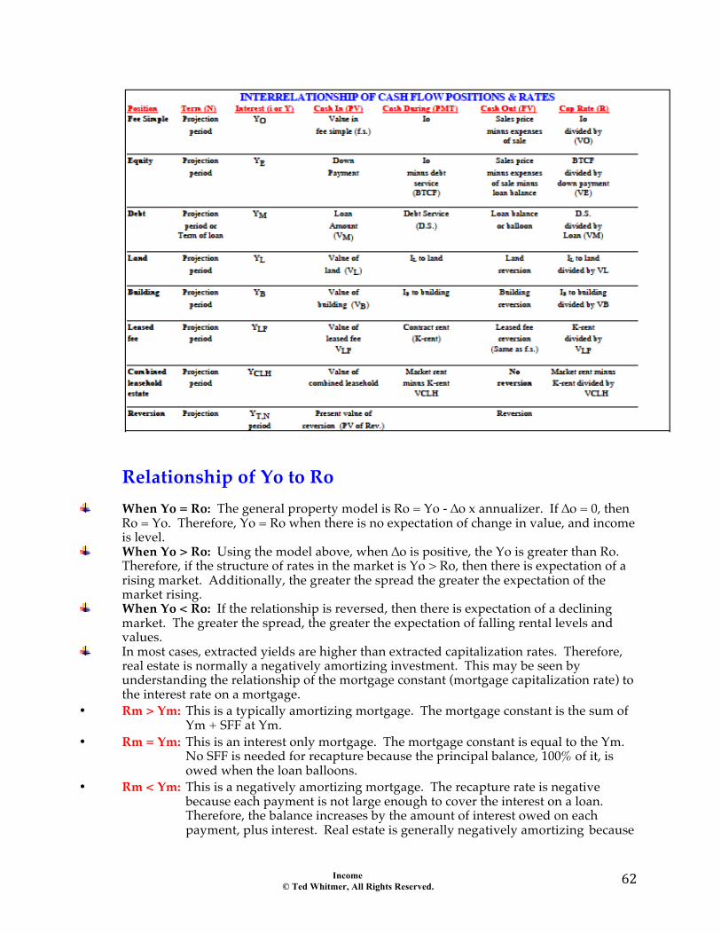
Relationship of Yo to Ro
When Yo = Ro: The general property model is Ro = Yo - ∆o x annualizer. If ∆o = 0, then Ro = Yo. Therefore, Yo = Ro when there is no expectation of change in value, and income is level.
When Yo > Ro: Using the model above, when ∆o is positive, the Yo is greater than Ro. Therefore, if the structure of rates in the market is Yo > Ro, then there is expectation of a rising market. Additionally, the greater the spread the greater the expectation of the market rising.
When Yo < Ro: If the relationship is reversed, then there is expectation of a declining market. The greater the spread, the greater the expectation of falling rental levels and values.
In most cases, extracted yields are higher than extracted capitalization rates. Therefore, real estate is normally a negatively amortizing investment. This may be seen by understanding the relationship of the mortgage constant (mortgage capitalization rate) to the interest rate on a mortgage.
• Rm > Ym: This is a typically amortizing mortgage. The mortgage constant is the sum of Ym + SFF at Ym.
• Rm = Ym: This is an interest only mortgage. The mortgage constant is equal to the Ym. No SFF is needed for recapture because the principal balance, 100% of it, is owed when the loan balloons.
• Rm < Ym: This is a negatively amortizing mortgage. The recapture rate is negative because each payment is not large enough to cover the interest on a loan. Therefore, the balance increases by the amount of interest owed on each payment, plus interest. Real estate is generally negatively amortizing because
Income © Ted Whitmer, All Rights Reserved.
63"
the Io is usually not enough to cover the Yo x Vo early in the investment. The "interest" accrues, which means the market expects the value and/or income to increase in the future.
The Ro is NIR ÷ EGIM. Therefore, as the EGIM increases, the Ro decreases. As Ro decreases the value increases. Higher EGIMs mean the market is willing to pay a higher multiple of income for a property.
Low Re (equity capitalization rates) mean there is an expectation of increasing income
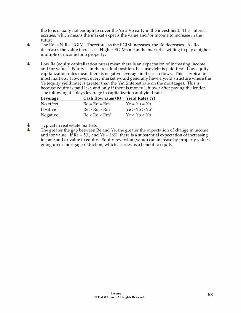
and/or values. Equity is in the residual position, because debt is paid first. Low equity capitalization rates mean there is negative leverage in the cash flows. This is typical in most markets. However, every market would generally have a yield structure where the Ye (equity yield rate) is greater than the Ym (interest rate on the mortgage). This is because equity is paid last, and only if there is money left over after paying the lender. The following displays leverage in capitalization and yield rates.
• Leverage Cash flow rates (R) Yield Rates (Y) • No effect Re = Ro = Rm Ye = Yo = Yo • Positive Re > Ro > Rm Ye > Yo > Yo* • Negative Re < Ro < Rm* Ye < Yo < Yo •
Typical in real estate markets The greater the gap between Re and Ye, the greater the expectation of change in income
and/or value. If Re = 5%, and Ye = 16%, there is a substantial expectation of increasing income and or value to equity. Equity reversion (value) can increase by property values going up or mortgage reduction, which accrues as a benefit to equity.
Income © Ted Whitmer, All Rights Reserved.
64"
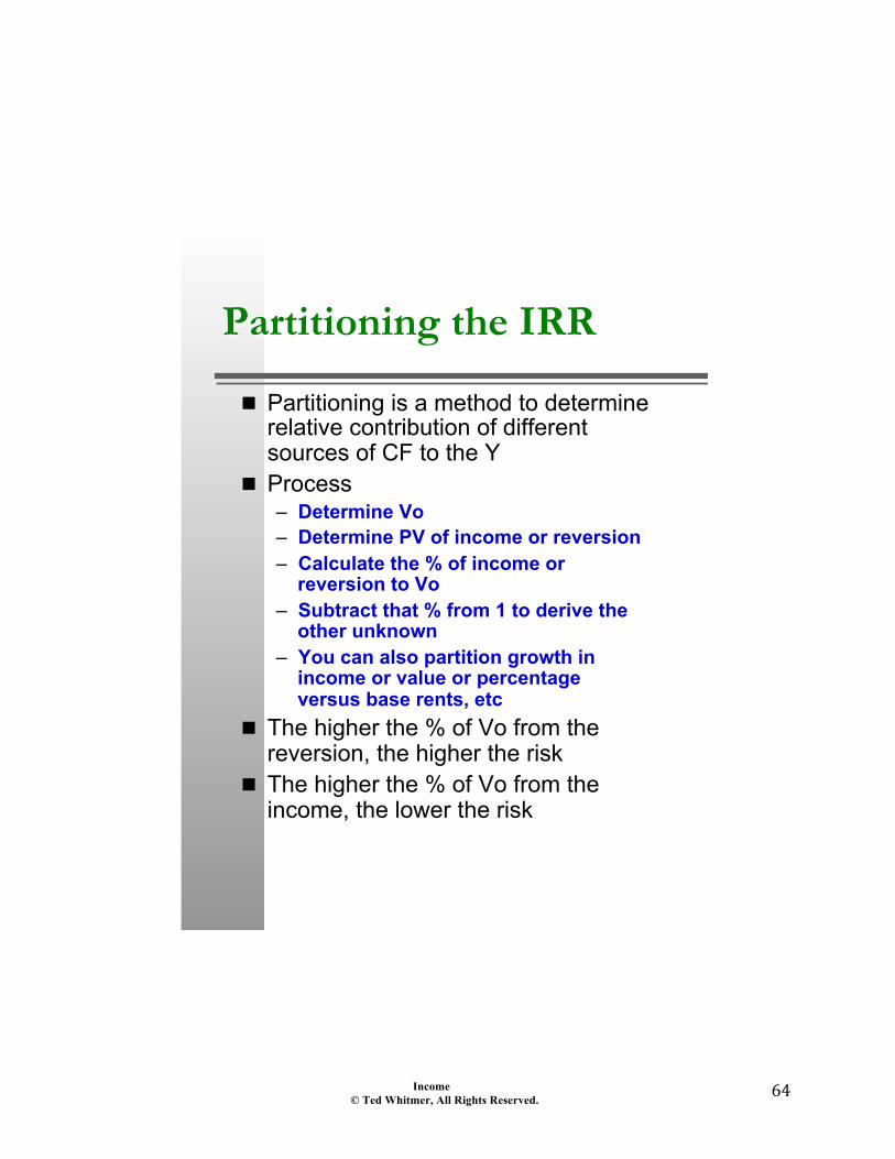
Partitioning the IRR
! Partitioning is a method to determine relative contribution of different sources of CF to the Y
! Process – Determine Vo – Determine PV of income or reversion – Calculate the % of income or
reversion to Vo – Subtract that % from 1 to derive the
other unknown – You can also partition growth in
income or value or percentage versus base rents, etc
! The higher the % of Vo from the reversion, the higher the risk
! The higher the % of Vo from the income, the lower the risk
Income © Ted Whitmer, All Rights Reserved.
65"
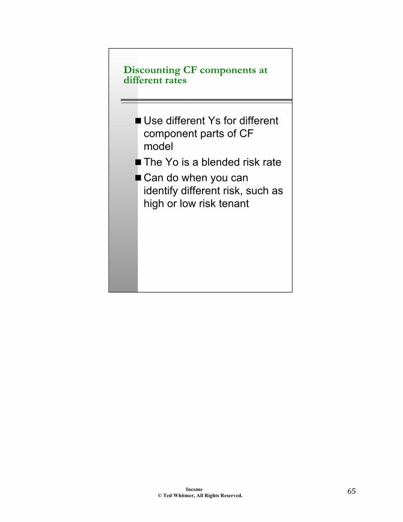
Discounting CF components at different rates
! Use different Ys for different component parts of CF model
! The Yo is a blended risk rate ! Can do when you can
identify different risk, such as high or low risk tenant
Income © Ted Whitmer, All Rights Reserved.
66"
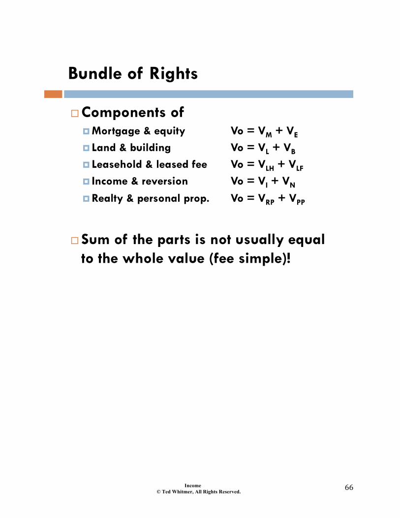
Bundle of Rights
! Components of ! Mortgage & equity Vo = VM + VE ! Land & building Vo = VL + VB ! Leasehold & leased fee Vo = VLH + VLF
! Income & reversion Vo = VI + VN ! Realty & personal prop. Vo = VRP + VPP
! Sum of the parts is not usually equal
to the whole value (fee simple)!