income hypothesis

8/7/2019 income hypothesis

http://slidepdf.com/reader/full/income-hypothesis 1/18

Stochastic Implications of the Life Cycle-Permanent Income Hypothesis: Theory and EvidenceAuthor(s): Robert E. HallSource: The Journal of Political Economy, Vol. 86, No. 6 (Dec., 1978), pp. 971-987Published by: The University of Chicago PressStable URL: http://www.jstor.org/stable/1840393 .

Accessed: 29/12/2010 09:32

Your use of the JSTOR archive indicates your acceptance of JSTOR's Terms and Conditions of Use, available at .

http://www.jstor.org/page/info/about/policies/terms.jsp. JSTOR's Terms and Conditions of Use provides, in part, that unlessyou have obtained prior permission, you may not download an entire issue of a journal or multiple copies of articles, and you

may use content in the JSTOR archive only for your personal, non-commercial use.

Please contact the publisher regarding any further use of this work. Publisher contact information may be obtained at .http://www.jstor.org/action/showPublisher?publisherCode=ucpress. .

Each copy of any part of a JSTOR transmission must contain the same copyright notice that appears on the screen or printed

page of such transmission.

JSTOR is a not-for-profit service that helps scholars, researchers, and students discover, use, and build upon a wide range of

content in a trusted digital archive. We use information technology and tools to increase productivity and facilitate new forms

of scholarship. For more information about JSTOR, please contact [email protected].

The University of Chicago Press is collaborating with JSTOR to digitize, preserve and extend access to The

Journal of Political Economy.

http://www.jstor.org

http://www.jstor.org/action/showPublisher?publisherCode=ucpress

http://www.jstor.org/stable/1840393?origin=JSTOR-pdf

http://www.jstor.org/page/info/about/policies/terms.jsp



http://www.jstor.org/page/info/about/policies/terms.jsp

http://www.jstor.org/stable/1840393?origin=JSTOR-pdf




Stochastic Implications of the LifeCycle-Permanent Income Hypothesis:Theory and Evidence

Robert E. HallCenterfor AdvancedStudyin theBehavioralSciencesandNationalBureauof EconomicResearch

Optimization of the part of consumersis shown to imply that the marginalutility of consumption evolves according to a random walk with trend.To a reasonable approximation, consumption itself should evolve in thesame way. In particular, no variable apart from current consumptionshould be of any value in predicting futureconsumption. This implicationis tested with time-series data for the postwar United States. It is con-firmed for real disposable income, which has no predictive power for

consumption, but rejected for an index of stock prices. The paper con-cludes that the evidence supports a modified version of the life cycle-permanent income hypothesis.

As a matter of theory, the life cycle-permanent income hypothesis is

widely accepted as the proper application of the theory of the consumer to

the problem of dividing consumption between the present and the future.

According to the hypothesis, consumers form estimates of their ability to

consume in the long run and then set current consumption to the appro-priate fraction of that estimate. The estimate may be stated in the form of

wealth, following Modigliani, in which case the fraction is the annuity value

of wealth, or as permanent income, following Friedman, in which case

the fraction should be very close to one. The major problem in empirical

research based on the hypothesis has arisen in fitting the part of the model

that relates current and past observed income to expected future income.

The relationship almost always takes the form of a fixed distributed lag,

though this practice has been very effectively criticized by Robert Lucas

(1976). Further, the estimated distributed lag is usually puzzlingly short.

Equations purporting to embody the life cycle-permanent income principle

This research was supportedby the National Science Foundation. I am gratefulto MarjorieFlavin for assistance and to numerous colleagues for helpful suggestions.[Journal of Political Economy, 1978, vol. 86, no. 6]

?) 1978 by The University of Chicago. 0022-3808/78/8606-0005$01.44

97I



972 JOURNAL OF POLITICAL ECONOMY

are actually little different from the simple Keynesian consumption func-

tion where consumption is determined by contemporaneousincome alone.

Much empirical researchis seriouslyweakened by failing to take proper

account of the endogeneity of income when it is the major independentvariable in the consumption function. Classic papers by Haavelmo (1943)

and Friedman and Becker (1957) showed clearly how the practice of

treating income as exogenous in a consumption function severely distorts

the estimatedfunction. Even so, regressionswith consumption as the depen-

dent variable continue to be estimated and interpretedwithin the life cycle-

permanent income framework.'

Though in principlesimultaneous-equationseconometrictechniquescan

be used to estimate the structural consumption function when its major

right-hand variable is endogenous, these techniques rest on the hypothesis

that certain observed variables, used as instruments, are truly exogenous

yet have an important influence on income. The two requirementsare often

contradictory, and estimation is based on an uneasy compromisewhere the

exogeneity of the instruments is uncertain. Furthermore,the hypothesis of

exogeneity is untestable.

This paper takes an alternative econometric approach to the study of

the life cycle-permanent income hypothesis by asking exactly what can be

learnedfrom a consumption regressionwhere it is conceded from the outset

that none of the right-hand variables is exogenous. This proceeds from a

theoretical examination of the stochastic implications of the theory. When

consumersmaximize expected futureutility, it is shown that the conditional

expectation of future marginal utility is a function of today's level of con-

sumption alone-all other information is irrelevant. In other words, apart

from a trend, marginal utility obeys a random walk. If marginal utility is a

linear function of consumption, then the implied stochastic properties of

consumption are also those of a random walk, again apart from a trend.Regression techniques can always reveal the conditional expectation of

consumptionor marginalutility given past consumption and any other past

variables. The strong stochastic implication of the life cycle-permanent

income hypothesisis that only consumption lagged one periodshouldhave a

nonzero coefficient in such a regression. This implication can be tested

rigorouslywithout any assumptionsabout exogeneity.

Testing of the theoretical implication proceeds as follows: The simplest

implication of the hypothesis is that consumption lagged more than oneperiod has no predictive power for current consumption. A more stringenttestableimplication of the random-walkhypothesisholds that consumptionis unrelated to anyeconomic variable that is observed in earlier periods. In

particular, lagged income should have no explanatory power with respectto consumption. Previous research on consumption has suggested that

' Examples are Darby 1972 and Blinder 1977.



LIFE CYCLE-PERMANENT INCOME HYPOTHESIS 973

lagged income might be a good predictor of current consumption, but this

hypothesis is inconsistent with the intelligent, forward-looking behavior of

consumers that forms the basis of the permanent-income theory. If the

previous value of consumption incorporated all information about the well-being of consumersat that time, then lagged valuesof actual income should

have no additional explanatory value once lagged consumption is included.The data support this view lagged income has a slightly negative co-efficient in an equation with consumption as the dependent variable andlagged consumption as an independent variable. Of course, contempo-

raneous income has high explanatory value, but thisdoes not contradict theprincipal stochastic implication of the life cycle-permanent income hy-

pothesis.As a final test of the random-walk hypothesis, the predictive power oflagged values of corporate stock prices is tested. Changes in stock prices

lagged by a single quarter are found to have a measurable value in predict-

ing changes in consumption, which in a formal sense refutes the simplerandom-walk hypothesis. However, the finding is consistent with a modifi-

cation of the hypothesis that recognizes a brief lag between changes inpermanent income and the corresponding changes in consumption. Thediscovery that consumption moves in a way similar to stock prices actuallysupportsthis modification of the random-walk hypothesis since stockprices

are well known to obey a random walk themselves.

The paper concludes with a discussion of the implications of the pure

life cycle-permanent income hypothesis for macroeconomic forecasting

and policy analysis. If every deviation of consumption from its trend is

unexpected and permanent, then the best forecast of future consumption is

just today's level adjusted for trend. Forecasts of future changes in incomeare irrelevant, since the information used in preparing them is already

incorporatedin today's consumption. In a forecasting model, consumptionshould be treated as an exogenous variable. For policy analysis, the purelife cycle-permanent income hypothesis supports the modern view that

only unexpected changes in policy affect consumption-everything knownabout future changes in policy is already incorporatedin present consump-tion. Further, unexpected changes in policy affect consumption only to the

extent that they affectpermanentincome, and then theireffectsareexpectedto be permanent. Policies that have a transitory effect on income are in-

capable of having a transitoryeffect on consumption. However, none of thefindingsof the paper implies that policies affectingincome have no effect on

consumption. For example, a permanent tax reduction generatesan imme-

diate increase in permanent income and thus an immediate increase in

consumption. But the evidence that policies act only through permanentincome certainly complicates the problem of formulating countercyclical

policies that act through consumption.




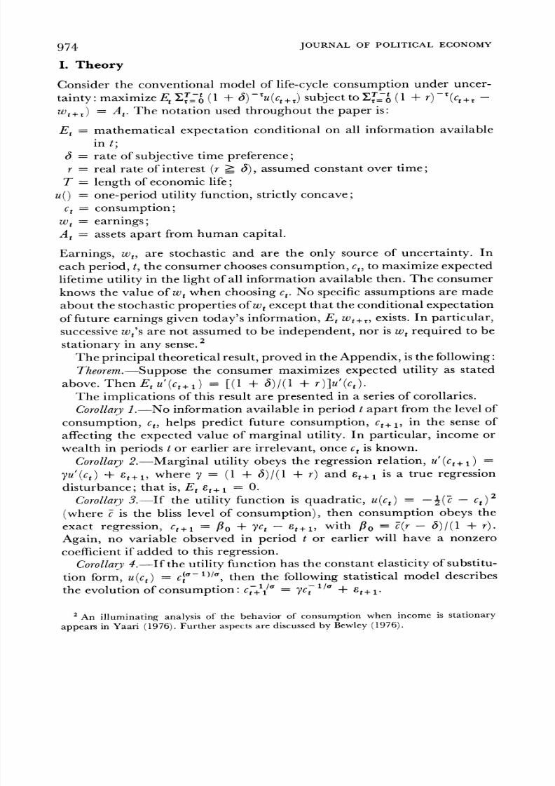
I. Theory

Consider the conventional model of life-cycle consumption under uncer-

tainty: maximize EtI` (1 + 3) -u(ct+,) subjectto ET_`7 (1 + r) -(ct+, -

Wt+r) = At. The notation used throughout the paper is:

Et = mathematical expectation conditional on all information available

in t;3 = rate of subjective time preference;

r = real rate of interest (r _ 3), assumed constant over time;

T = length of economic life;

u() = one-period utility function, strictly concave;

ct= consumption;t= earnings;

At= assetsapart from human capital.

Earnings, wt. are stochastic and are the only source of uncertainty. In

each period, t, the consumerchoosesconsumption,ct,to maximize expected

lifetime utility in the light of all information available then. The consumer

knows the value of wtwhen choosing ct. No specific assumptionsare made

about the stochasticpropertiesof wt except that the conditional expectation

of future earningsgiven today's information, Et wt+ , exists. In particular,successivewe'sare not assumed to be independent, nor is wtrequired to be

stationary in any sense.2

The principal theoreticalresult,provedin the Appendix, is the following:

Theorem. Suppose the consumer maximizes expected utility as stated

above. Then Et u'(ct+1) = [(1 + 3) /(1 + r)]u'(ct).

The implications of this result are presented in a seriesof corollaries.

Corollary1. No information available in period t apart from the level of

consumption, ct. helps predict future consumption, ct+1, in the sense ofaffecting the expected value of marginal utility. In particular, income or

wealth in periods t or earlier are irrelevant, once ct is known.

Corollary2.-Marginal utility obeys the regressionrelation, u'(ct+ ) =

yu'(ct) + et+,, where y = (1 + 6)/(1 + r) and et+1 is a true regression

disturbance; that is, Et Et+1 = ?.

Corollary3. If the utility function is quadratic, u(ct) = -2(-c

(where c is the bliss level of consumption), then consumption obeys the

exact regression, ct+1 =

P3o+ yct - et+ , with fl = c(r - 3)/(1 + r).

Again, no variable observed in period t or earlier will have a nonzero

coefficient if added to this regression.

Corollary4.-If the utility function has the constant elasticity of substitu-

tion form, u(ct) = cta-1)1', then the following statistical model describes

the evolution of consumption: cT+'11" - 1y /a + t+i1

2 An illuminating analysis of the behavior of consumption when income is stationary

appears in Yaari (1976). Further aspects are discussed by Bewley (1976).




Corollary5. Suppose that the change in marginal utility from oneperiod to the next is small, both because the interestrate is close to the rate

of time preference and because the stochastic change is small. Then

consumption itself obeys a random walk, apart from trend.3 Specifically,ct+1= Atct+ et+1/u"(ct)+ higher-order terms where A, is [(1 + 3)/(1 + r)] raised to the power of the reciprocal of the elasticity of marginal

utility

= 1 + 3 )UZ(ct)ICtU",(Ct)

1 +r

The rate of growth, i, exceeds one because u"is negative. It may change

over time if the elasticity of marginal utility depends on the level of con-sumption. However, it seems likely that constancy of A, will be a good

approximation, at least over a decade or two. Further, the factor 1/u"(C,)in the disturbance is of little concern in regressionwork-it might introduce

a mild heteroscedasticity, but it would not bias the resultsof ordinary least

squares. From this point on, Et will be redefined to incorporate I/u"(ce)

where appropriate.

This line of reasoning reaches the conclusion that the simple relationship

Ct=

ict- 1+ Et where

1,is

unpredictableat time t -

1,is a close

approxi-mation to the stochastic behavior of consumption under the life cycle-

permanent income hypothesis. The disturbance,E, summarizes the impact

of all new information that becomes available in period t about the con-

sumer's lifetime well-being. Its relation to other economic variables can be

seen in the following way. First, assets, A,, evolve according to A, =

(1 + r)(At,1 - c1 + wt_1). Second, let Ht be human capital,

defined as current earnings plus the expected present value of future

earnings: HL= I[`o (1 + r)-T Et wt+ where Et wt = wt.Then Ht evolves

according to Ht = (1 + r)(II_1-Hwt 1) + I' -7 (1 + r)-'(Et wt~ -

Etw 1 Wt+T). Let qt be the second term, that is, the present value of the set

of changes in expectations of future earningsthat occur between t - 1 and

t. Then by construction, Et_ 1qt = 0. Still, the first term in the expressionfor Ht may introduce a complicated intertemporal dependence into its

stochasticbehavior; only under very special circumstanceswill it be a ran-

dom walk. The implied stochastic equation for total wealth is At + Ht =

(1 + r)(At-1 + H,1 - ct-1) + rtt The evolution of total wealth then

depends on the relationshipbetween the new information about wealth, It,

and the induced change in consumption as measuredby Et. Under certaintyequivalence, justified either by quadratic utility or by the small size of Et,

the relationshipis simple: Et = [1 + i/l(l + r) + *.. + T t/l(l + r)T-t]17t

= Xtqt This is the modified annuity value of the increment in wealth. The

3Granger and Newbold (1976) present much stronger results for a similar problem but

assume a normal distribution for the disturbance.




modification takes account of the consumer'splans to make consumption

grow at proportional rate A over the rest of his life. Then the stochastic

equationfortotalwealthisA, + H, = (1 + r)(1 -at1)(A, 1 + H,.1)

+ C, which is a random walk with trend.Consumers, then, process all available information each period about

current and futureearnings. They convertdata on earnings, which may have

large, predictable movements over time, into human capital, which evolves

according to a combination of a highly predictable element associatedwith

the realization of currentearnings and an unpredictable element associated

with changing expectationsabout futureearnings. Taking account as well of

financial assets accumulated from past earnings, consumers determine an

appropriate current level of consumption. As shown at the beginning of this

section, this implies that marginal utility evolves as a random walk with

trend. As a result of consumers' optimization, wealth also evolves as a

random walk with trend. Although it is tempting to summarize the theory by

saying that consumption is proportional to wealth, wealth is a random

walk, and so consumption is a random walk, this is not accurate. Rather,

the underlying behavior of consumers makes both consumption and wealth

evolve as random walks.

All of the theoretical results presented in this section rest on the assump-

tion that consumers face a known, constant, real interest rate. If the real

interest rate varies over time in a way that is known for certain in advance,

the results would remain true with minor amendments-mainly, A, would

vary over time on this account. The importance of known variations in

interest rates depends on the elasticity of substitution between the present

and future. If that elasticity is low, the influence would be unimportant.

On the other hand, if the real interest rate applicable between periods t

and t + 1 is uncertain at the time the consumption decision in period t

is made, then the theoretical results no longer apply. However, there seemsno strong reason for this to bias the results of the statistical tests in one

direction or another.

II. Tests to Distinguish the Life Cycle-Permanent Income Theory

from Alternative Theories

The tests of the stochastic implications of the life cycle-permanent income

hypothesis carried out in this paper all have the form of estimating a condi-tional expectation, E(c I Ct_1, xt- 1i), where xt- 1 is a vector of data known

in period t - 1, and then testing the hypothesis that the conditional expecta-

tion is actually not a function of x, 1- 4 In all cases, the conditional expecta-

4 The nature of the hypothesis being tested and the statistical tests themselves are essentially

the same as in the large body of research on efficient capital markets (see Fama 1970). Sims

(1978) treats the statistical problem of the asymptotic distribution of the regression coefficients

of x,- 1 in this kind of regression, with the conclusion that the standard formulas are correct.




tion is made linear in xt- 1, so the tests are the usualF-tests for the exclusion

of a group of variables from a regression. Again, regressionis the appro-

priate statistical technique for estimating the conditional expectation, and

no claim is made that the truestructuralrelation between consumption andits determinants is revealed by this approach.

What departuresfrom the life cycle-permanent income hypothesis will

this kind of test detect? There are two principal lines of thought about

consumption that contradict the hypothesis. One holds that consumersare

unableto smoothconsumptionovertransitoryfluctuationsin incomebecause

of liquidity constraintsand other practical considerations.Consumption is

therefore too sensitive to current income to conform to the life cycle-per-

manent incomeprinciple. The second holds that a reasonable measureof

permanentincome isa distributedlagof pastactual income, so theconsump-

tion function should relate actual consumption to such a distributed lag.

A general consumptionfunction embodying both ideas might let consump-

tion respondwith a fairly large coefficientto contemporaneousincome and

then have a distributed lag over past income. Such consumption functions

are in widespread use and fit the data extremely well. But their estimation

involves the very substantial issuethat income and consumption arejointly

determined. Estimation by least squaresprovides no evidence whether the

observed behavior is consistent with the life cycle-permanent income

hypothesis or not. Simultaneous estimation could provide evidence, but it

would rest on crucialassumptionsof exogeneity. Regressionsofconsumption

on lagged consumption and lagged income can provide evidence without

assumptionsof exogeneity, as this section will show.

Considerfirst the issueof excessivesensitivityof consumptionto transitory

fluctuations in income, which has been emphasized by Tobin and Dolde

(1971) and Mishkin (1976). The simplest alternative hypothesis supposes

that a fractionof the population simplyconsumesall of itsdisposableincome,instead of obeying the life cycle-permanent income consumption function.

Suppose this fraction earnsa proportion ji of total income, and let c' = puyt

be their consumption. The other part of consumption, say ct, follows the

rule set out earlier: C"= W'_ 1 + 6t. The conditional expectation of total

consumption, ct.given its own lagged value, and, say, two lagged valuesof

income, is E(ct ICt- 1,Yt- l,Yt- 2) = E(ct ICt- 1,Yt- 1,Yt- 2 ) + E(c' Ic, 1,

Yt-1,Yt-2) = HE(yt It- IYt1,Yt- 2) + A(ct1 - /PYt-l). Suppose that

disposableincome obeys a univariateautoregressiveprocessof secondorder,so E(yt Ct-1,Yt-1,Yt-2) = PlYt-l + P2Yt-2. Then E(ct Ict,1,yt-l,

Yt- 2) = Act-1 + !(P1 -i) Yt-I + PP2Yt-2. The life cycle-permanentincome hypothesis will be rejected unless P =-i and P2 = 0, that is,

unlessdisposable income and consumptionobey exactly the same stochastic

process. If they do, permanent income and observed income are the same

thing, and the liquidity-constrained fraction of the population is obeying

the hypothesis anyway, so the hypothesis is confirmed. The proposed test




involving regressing c, on c, 1,yt- 1, andYt 2 will reject the life cycle-permanent income hypothesis in favor of the simple liquidity-constrainedmodel whenever the latter is materially different from the former.

The distributed lag approximation to permanent income was first sug-gested by Friedman (1957, 1963) and has figuredprominently in consump-tion functions ever since. Distributed lags are not necessarily incompatiblewith the life cycle-permanent income hypothesis if income obeys a stable

stochastic process,there should be a structural relation between the innova-tion in income and consumption (Flavin 1977).5 Still, the theory of theconsumer presented earlier rules out any extra predictive value of a dis-tributed lag of income (excluding contemporaneousincome) in a regressionthat contains lagged consumption. If consumers use a nonoptimal distri-buted lag in formingtheir estimates of permanent income, then this centralimplication of the life cycle-permanent income hypothesis is false. Thisproposition is easiest to establish for the simple Koyck or geometric distri-buted lag, ct = oX/i 3fl5t-i or t = flc, + ocy Suppose, as before,

thaty, obeys a second-orderautoregressiveprocess,E(y, ICt- 1,Yt- 1,Yt- 2)

= PlYt-1 + P2Yt-2. Then the conditional expectation is E(ct Ict-1,Yt- 1,Yt- 2) = f3Ct- 1 + pY t- 1 + (P2Yt- 2. As long as income is seriallycorrelated (P, # 0 or P2 = 0), this conditional expectation will not

depend solely on c, 1and the pure life cycle-permanent income hypothesiswill be refuted. Discussion of the peculiarities of the case of uncorrelatedincome seems unnecessary since income is in fact highly serially correlated.With thisslightqualification,theproposedtestprocedurewillalwaysdetectaKoyck lag if it is present and thus refute the life cycle-permanent income

hypothesis.

It is possible to show that the test also applies to the general distributed

lag model used by Modigliani (197 1) and others.If the lag in the underlying

structural consumption function is nonoptimal, lagged income will haveadditional predictive power forcurrentconsumption beyond that of lagged

consumption,sothelifecycle-permanent income hypothesiswill be rejected.Data generated by consumerswho use an optimal distributedlag of current

and past income in making consumption decisionswill not cause rejection.This shows the crucial distinction between structural models which include

contemporaneous income and the test regressionsof this paper where the

principle of the tests involves the inclusion of lagged variablesalone.

This section has shown that simple tests of the predictive power of vari-ables other than lagged consumption can detect departuresfrom the purelifecycle-permanent income hypothesisin the two directionsthat have been

widely suggested in previous research on consumption. Both excessivesensitivity to current income because of liquidity constraints and non-

5 Lucas (1976) argues convincingly that the stochastic process for income will shift if

policy rules change.




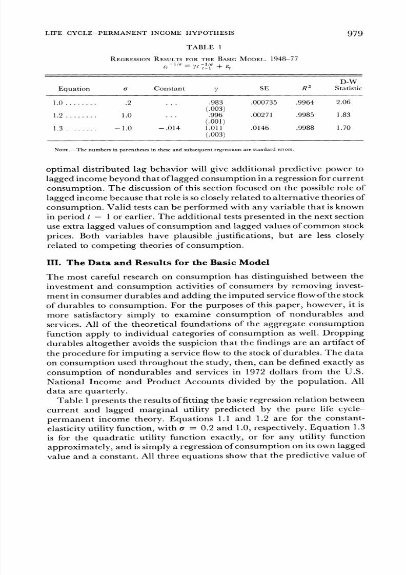
TABLE 1

REGRESSION RESULTS FOR THE BASIC MODEL.. 1948-77-Ila= ycl/a + g

D-WEquation a Constant y SE R2 Statistic

1.0 ....... .2 ... .983 .000735 .9964 2.06(.003)

1.2 ....... 1.0 ... .996 .00271 .9985 1.83(.001)

1.3 ....... - 1.0 -.014 1.011 .0146 .9988 1.70(.003)

NoTE.-The numbersin parenthesesin these and subsequent regressionsare standard errors.

optimal distributed lag behavior will give additional predictive power to

lagged income beyond that of lagged consumptionin a regressionforcurrent

consumption. The discussionof this section focused on the possible role of

lagged income because that role is so closely relatedto alternative theoriesof

consumption. Valid tests can be performedwith any variable that is known

in period t - 1or earlier.The additional testspresentedin the next section

use extra lagged values of consumption and lagged values of common stock

prices. Both variables have plausible justifications, but are less closelyrelated to competing theoriesof consumption.

III. The Data and Results for the Basic Model

The most careful research on consumption has distinguished between the

investment and consumption activities of consumers by removing invest-

ment in consumerdurablesand adding the imputed serviceflowof the stock

of durables to consumption. For the purposesof this paper, however, it is

more satisfactory simply to examine consumption of nondurables andservices. All of the theoretical foundations of the aggregate consumption

function apply to individual categories of consumption as well. Dropping

durables altogether avoids the suspicion that the findings are an artifactof

the procedureforimputing a serviceflow to the stockof durables. The data

on consumption used throughout the study, then, can be defined exactly as

consumption of nondurables and services in 1972 dollars from the U.S.

National Income and Product Accounts divided by the population. All

data are quarterly.Table 1presentsthe resultsof fitting the basic regressionrelationbetween

current and lagged marginal utility predicted by the pure life cycle-

permanent income theory. Equations 1.1 and 1.2 are for the constant-

elasticity utility function, with a = 0.2 and 1.0, respectively. Equation 1.3

is for the quadratic utility function exactly, or for any utility function

approximately, and is simply a regressionof consumption on its own lagged

value and a constant. All three equations show that the predictive value of




lagged marginal utility forcurrentmarginalutility is extremelyhigh; that is,

the typical informationthat becomes available in each quarter, as measured

by et, hasonly a small impact on consumptionor marginalutility. Of course,

this is no more than a theoretical interpretationof the well-known fact thatconsumption is highly serially correlated. The close fit of the regressionsin

table 1 is not itself confirmation of the life cycle-permanent income hy-

pothesis, since the hypothesis makes no prediction about the variability of

permanentincome and the resultantvarianceofsE. The theoryis compatible

with any amount of unexplained variation in the regression.

There is no usable statistical criterion for choice among the three equa-

tions in table 1. The transformationof the dependent variable rulesout the

simple principle of least squares. Under the assumptionof a normal distri-

bution foret, there is a likelihoodfunction with an extra term, theJacobian

determinant, to take account of the transformation. However, for this

sample, it proved to be an increasing function of a for all values, so no

maximum-likelihoodestimatoris available. This seems to reflect the opera-

tion of corollary 5 the yet'sare small enough that any specification of

marginal utility is essentially proportional to consumption itself, and the

effective content of the life cycle-permanent income theory is to make con-

sumption itself evolve as a random walk with trend. From this point on,

the paper will discussonly equation 1.3 and its extensionsto other variables.The principal stochastic implication of the life cycle-permanent income

hypothesis is that no other variables observed in quarter t - 1 or earlier

can help predict the residuals from the regressionsin table 1. Beforeformal

statistical tests are used, it is useful to study the residuals themselves. The

pattern of the residualsis extremelysimilar in the three regressions,but the

residualsthemselvesare easiest to interpret for equation 3, where they have

the units of consumption per capita in 1972 dollars. These residualsappear

in table 2.The standard errorof the residualsin 14.6, so roughly six of the observa-

tions should exceed 29.2 in magnitude. There are in fact six. Three are

drops in consumption, and of these, one coincides with the standarddating

of recessions: 1974:4. Five milder recessionscontribute drops of less than

two standard deviations: 1949:3, 1953:4, 1958:1, 1960:3, and 1970:4.

The other major decline in consumption is associated with the Korean

War, in 1950:4. Most of the dropsin consumptionoccurredquickly, in one

ortwo quarters.The only importantexceptionwas in the periodfrom 1973:4to 1975: 1, when six straight quartersof consecutive decline took place. On

the expansionary side, there is little consistent evidence of any systematictendency for consumption to recover in a regular pattern after a setback.

The largest single increase occurred in 1965:4. This, together with three

successiveincreasesin 1964, accounts for all of the increase in consumption

relative to trend associated with the prolonged boom of the mid- and late

sixties.



LIFE CYCLE-PERMANENT INCOME HYPOTHESIS 98 I

TABLE 2

RESIDUALS FROM REGRESSION OF CONSUMPTION ON LAGGED CONSUMPTION, 1948-77 ($)

1948: 1956: 1964: 1972:

1.... .5 1.... 2.8 1.... 17.8 1.... 20.02.... 8.0 2.. .. -10.1 2.... 20.0 2... 32.73.... - 15.5 3.... -6.1 3.... 14.6 3.... 8.44.... 3.5 4.... 1.2 4.... -4.4 4.... 21.1

1949: 1957: 1965: 1973:1.... -8.6 1.... - 10.8 1.... 5.8 1 .... 8.02.... -8.5 2.. .. -6.1 2.... 5.2 2.... - 15.63.... - 27.2 3.... 2.4 3.... 10.2 3 .... 3.04.... -.1 4.... - 13.6 4.... 38.7 4.... -32.8

1950: 1958: 1966: 1974:1.... 5.6 1.... -29.1 1.... - 1.3 1.... -27.32.... 23.8 2 .... 8.3 2.... 3.7 2-... - 23.4

3.... 15.5 3 .... 14.3 3.... - 1.9 3.... - 16.64.... - 31.0 4.... - 1.9 4.... - 12.4 4.... - 42.81951: 1959: 1967: 1975:

1 .... 16.0 1.... 15.1 1.... 10.2 1.... -5.82.... - 24.8 2.... 3.8 2.... 2.0 2 .... 25.63 .... 9.0 3.... -2.7 3.... -2.8 3.... -21.34.. . - 6.1 4.. 4.. 1.1 4.... - 7.5 4.... .9

1952: 1960: 1968: 1976:1.... - 15.1 1.... -5.6 1.... 15.6 1.... 24.42.... 18.0 2.... 8.8 2.... 7.9 2.... 8.33.... 10.0 3.... - 24.3 3.... 22.2 3.... 2.34.... 8.6 4.... - 10.1 4.... -8.1 4.... 30.4

1953: 1961: 1969: 1977:1.... - 1.6 1 .... 1.8 1.... .8 1.. -1.82.... - 1.0 2.... 10.1 2.... -5.33.... -22.1 3.... - 16.9 3.... -2.44.... - 27.0 4.... 15.8 4.... .3

1954: 1962: 1970:1.... -.1 1.... -1.7 1,... 4.02.... -2.4 2 .... 3.4 2.... - 12.33.. . 11.9 3.... - .8 3. . . .-34.... 7.4 4.... .6 4.... -21.5

1955: 1963: 1971:1.... 6.1 1.... -8.4 1.... 1.52.... 7.0 2.... - 1.3 2.... - 2.4

3.... -.8 3 .... 11.7 3.... - 14.64.... 22.3 4.... -6.3 4.... -6.6

The data contain no obvious refutation of the unpredictability of the

residualsfrom the basic model, but, just as a study of stockpriceswill never

convince the "chartist"that it is futile to try to predict their future, the con-

firmed believer in regular fluctuations in consumption will not be swayed

by the data alone. More powerful methods for summarizing the data are

required.

IV. Can Consumption Be Predicted from Its Own Past Values?

The simplest testable implication of the pure life cycle-permanent income

hypothesis is that only the first lagged value of consumption helps predictcurrent consumption. This implication would be refuted if consumptionhad a definite cyclical pattern described by a difference equation of second




or higher order.6 Intelligent consumersought to be able to offset any such

cyclical pattern and restorethe noncyclical optimal behavior of consump-

tion predicted by the hypothesis. The following regressiontests this implica-

tion by adding additional lagged values of consumption to equation 1.3:

Ct= 8.2 + 1*130ct- - 0.040ct- 2 + 0.030c 3 - 0.lIl3c, 4;

(8.3) (0.092) (0.142) (0.142) (0.093)

R2= .9988; s = 14.5; D-W = 1.96.

The contribution of the extra lagged values is to increase the accuracy of

the forecastof current consumption by about 10 cents per person per year.

The F-statistic for the hypothesis that the coefficients of ct-2,Ct2 3, and

ct 4 are all zero is 1.7, well underthe critical point of the F-distributionof

2.7 at the 5 percent level. Only very weak evidence against the pure life

cycle-permanent income hypothesis appears in this regression.In particu-

lar, there are no definite signs that consumption obeys a second-order

difference equation capable of generating stochastic cycles. In this respect,

consumption differs sharply from other aggregate economic measures,

which do typically obey second-orderautoregressions.

V. Can Consumption Be Predicted from Disposable Income?

If lagged income has substantial predictive power beyond that of lagged

consumption, then the life cycle-permanent income hypothesis is refuted.

As discussed in Section II, this evidence would support the alternative

views that consumersare excessively sensitive to current income, or, more

generally, that they usean ad hoc, nonoptimal distributedlag of pastincome

in making consumption decisions.

Table 3 presents a variety of regressionstesting the predictive power of

real disposable income per capita, measured as current dollar disposableincome from the national accounts divided by the implicit deflator for

consumption of nondurables and services and divided by population.

Equation 3.1 shows that a single lagged level of disposable income has

essentially no predictive value at all. The coefficient of y, is slightly

negative, but this is easily explained by sampling variation alone. The

F-statistic for the exclusion of all but the constant and ct- 1 is 0.1, far below

the critical Fof 3.9. Equation 3.2 triesa year-longdistributedlag estimated

without constraint. The firstlagged value of disposable income has a slight

positive coefficient, but this is more than outweighed by the three negative

coefficients for the longer lags. The long-run "marginal propensity to

consume," measured by the sum of the coefficients, is actually negative,

though again this could easily result from sampling variation. The F-

statistic for the joint predictive value of all four lagged income variables is

2.0, somewhat less than the critical value of 2.4 at the 5 percent level. Note

6 Fama (1970) calls the similar test for asset prices a "weak form" test.



0-4 0'4

C4 014

P4~~~~~~~~~0

~~~40

00W.) v

0li 0)

co"I-T

~~~~~~0 ~ ~ ~ ~ ~~c

(O COdz o

H0 om s

: C CL. m.m.~~~~CDC'

CZ0 I

X - Ico

0 .

*.9 I

.' ..I

0 ~ C rI~0 -e r-CO

Q e -98




that the pure life cycle-permanent income hypothesis would be rejectedif

the size of the test were 10 percent or higher.

Equation 3.3 fits a 12-quarterAlmon lag to see if a long distributed lag

can compete with lagged consumption as a predictor for currentconsump-tion. Again, the sum of the lag coefficientsis slightly negative, now almost

significantly so. The F-statistic for the hypothesis of no contribution from

the complete distributed lag on income is again close to the critical value.

The sample evidence of the relation between consumption and lagged

income seems to say the following: There is a statistically marginal and

numerically small relation between consumption and very recent levels of

disposable income. The sum of the lag coefficients is slightly negative.

Further,thereisno evidence atall

supportingthe view thata longdistributed

lag coveringseveralyearshelps to predict consumption. This evidence casts

just a little doubt on the life cycle-permanent income hypothesisin itspurest

form but is not at all destructiveto a somewhat moreflexible interpretation

of the hypothesis, to be discussedshortly.

VI. Wealth and Consumption

Of the many alternativevariablesthat might be included on the right-hand

side of a regressionto test the pure life cycle-permanent income hypothesis,

some measure of wealth is one of the leading candidates. Theory and pre-

vailing practice agree that contemporaneouswealth has a strong influence

on consumption, so lagged wealth is a logical variable to test. Again, the

hypothesis implies that wealth measuredin earlierquartersshould have no

predictivevalue with respectto this quarter'sconsumption.All information

contained in lagged wealth should be summarized in lagged consumption.

Reliable quarterly data on property values are not available for most

categoriesof property. For one majorcategory, however, essentiallyperfectdata are available at any frequency, namely, the market value of corporate

stock. Tests of the random-walkhypothesisdo not requirea comprehensive

wealth variable, so a test based on stock prices is appropriate, even though

the resulting equation does not describe the structural relation between

wealth and consumption. The tests reportedhere arebasedon Standardand

Poor's comprehensive index of the prices of stocksdeflated by the implicit

deflatorfor nondurablesand servicesand divided by population. This vari-

able will be called s. It makes a statistically unambiguous contribution toprediction of current consumption:

t = -22 + 1.012ct-i + 0.223st1 - 0.258st2 + 0.167s,-3- 0.120st-4(8) (0.004) (0.051) (0.083) (0.083) (0.051)

R2 = .9990; SE = 14.4; D-W = 2.05.

The F-statistic for the hypothesis that the coefficients of the lagged stock

prices are all zero is 6.5, well above the critical value of 2.4 at the 5 percent




level. Further, each coefficient considered separately is clearly different

from zero according to the usual t-test. However, the improvement in the

predictive power of the regression, while statistically significant, is not

numerically large. The standard error of the regression is about 20 centsper person per year smaller in this equation compared with the basic model

of equation 1.3 ($14.40 against $14.60). Most of the predictive value of thestock price comes from the changein the price in the immediately preceding

quarter. A smaller contribution is made by the change in the price 3

quarters earlier. Use of the Almon lag technique for both levels and differ-

ences in the stock price failed to turn up any evidence of a longer distributed

lag.

VII. Implications of the Empirical Evidence

The pure life cycle-permanent income hypothesis that ctcannot be pre-

dicted by any variable dated t - 1 or earlier other than ct- 1 is rejected

by the data. The stock market is valuable in predicting consumption 1quarter in the future. Most of the predictive power comes from As, 1. But

the data seem entirely compatible with a modification of the hypothesis

that leaves its central content unchanged. Suppose that consumption does

depend on permanent income, and that marginal utility indeed does evolve

as a random walk with trend, but that some part of consumption takes time

to adjust to a change in permanent income. Then any variable that is

correlated with permanent income in t - 1 will help in predicting the

change in consumption in period t, since part of that change is the laggedresponse to the previous change in permanent income. Both the finding that

consumption is only weakly associated with its own past values and that

immediate past values of changes in stock prices have a modest predictive

value are compatible with this modification of the life cycle-permanentincome hypothesis.

Whatever problems remain in the consumption function, there seems

little reason to doubt the life cycle-permanent income hypothesis. Within

a framework in which permanent income is treated as an unobserved

variable the data seem fully compatible with the hypothesis, provided a

short lag between permanent income and consumption is recognized. Of

course,acceptance of the hypothesisdoes not yield a complete consumption

function, since no equation forpermanent income has been developed. Theevidenceagainstthe ad hocdistributed-lagmodelrelating permanentincome

to actual income seems fairly strong. The task of further research is to

create a moresatisfactorymodel forpermanent income, one that recognizesthat consumers appraise their economic well-being in an intelligent waythat involves looking into the future.

It is important not to treat any of the equationsof this paper asstructural

relationsbetween consumption and the variablesthat are used to predict it.




For example, table 3 should not be read as implying that income has a

negative effect on consumption. The effect of a particular change in income

depends on the change in permanent income it induces, and this can range

anywhere from no effect to a dollar-for-dollareffect, depending on the waythat consumersevaluate the change. In any case, the regressionsunderstate

the true structural relationbetween the change in income and the change in

consumption because they omit the contemporaneouspart of the relation.

VIII. Implications for Forecasting and Policy Analysis

Under the pure life cycle-permanent income hypothesis, a forecast of

future consumption obtained byextrapolatingtoday's level by the historical

trend is impossible to improve. The results of this paper have the strong

implication that beyond the next few quarters consumption should be

treated as an exogenous variable. There is no point in forecasting future

income and then relating it to income, since any information available

today about future income is already incorporated in today's permanent

income. Forecasts of consumption next quarter can be improved slightly

with current stock prices, but no further improvement can be achieved in

this way in later quarters.

With respect to the analysis of stabilization policy, the findings of thispaper go no furtherthan supportingthe view thatpolicy affectsconsumption

only as much as it affectspermanent income. In the analysisof policies that

are known to leave permanent income unchanged, consumption may be

treated as exogenous. Further, only new information about taxes and other

policy instruments can affect permanent income. Beyond these general

propositions, the policy analyst must answer the difficult question of the

effect of a given policy on permanent income in order to predict its effect

on consumption. Regressionof consumption on current and past values ofincome are of no value whatsoever in answering this question.

Appendix

1. Theorem

If a consumer maximizes Et '= o (1 + 3) -tu(c,), subject to E' o (1 + r) -t(ct - i)

= A0, sequentially determining c, at each t, then Etu'(c,+1) = [(1 + 6)/(1 + r)]x u'(ct).

Proof.-At time t, the consumer chooses ct so as to maximize (1 + 6) -tu(cq) +

Et -r'=,+1 (1 + 3)-tu(c,) subject to I' , (1 + r)(T-t)(c, - w,) = A,. The optimal

sequential strategy has the form c, = g, (wt,.w ,.-. ., wO,AO). Consider a variation

from this strategy: ct = gtw, . * **) + x: t+1 = gt + I (w + 1, wt,. * (1 + r)x.

Note that the new consumption strategy also satisfies the budget constraint. Now

consider maxx{(1 + 6)-tu(g, + x) + Et [(1 + 6)-t-u(g,,, - (1 + r)x) +

,?=t+2 (1 + c) yu(gr)]}-The first-order condition is (1 + 6) -tu'(gt + x) - Et (1 + 6>)t'(l + r)

U'(g, + I - (1 + r)x) = 0 as asserted.




2. Proof of Corollary5

Recall that u'(ct+,) = [(1 + 6)/(1 + r)]u'(ct) + et+l and At = [(1 + 3)/

(1 + r)]u'(ct)I(ctu"(ct)].Expand the implicit equation for ct+ 1 in a Taylor series at the

pointAt = 1 (r = 6) andet+ 1 = :ct + 1 = ct + (t - 1) (act+ 1/aAt) + et + 1(act + I/

08t + 1) + higher-order terms. At the point A, = 1and et + 1 = 0, ct+ 1 equals ct,andit is not hard to show that act+1/IAt = ct and act+1it+1 = l/u"(c,). Thus c,+1 =

c, + (i - l)c + et+1/u"(ct) = tct++ et+1l/u"(ct), as asserted.

References

Bewley, Truman. "The Permanent Income Hypothesis: A Theoretical Formula-

tion." Mimeographed. Cambridge, Mass.: Harvard Univ., Dept. Econ.,

September 1976.Blinder, Alan. "Temporary Taxes and Consumer Spending." Mimeographed.

Jerusalem: Inst. Advanced Studies, April 1977.

Darby, Michael R. "The Allocation of Transitory Income among Consumers'

Assets." A.E.R. 62 (December 1972): 928-41.

Fama, Eugene F. "Efficient Capital Markets: A Review of Theory and Empirical

Work." J. Finance 25 (May 1970): 383-417.

Flavin, Marjorie. "The Adjustment of Consumption to Changing Expectations

about Future Income." Unpublished paper, Massachusetts Inst. Tech., February

1977.

Friedman, Milton. A Theory of the ConsumptionFunction. Princeton, NJ.: PrincetonUniv. Press, 1957.

. "Windfalls, the 'Horizon,' and Related Concepts in the Permanent-

Income Hypothesis." In Measurement in Economics: Studies in Mathematical Eco-

nomicsand Econometricsin Memory of Yehuda Grunfeld,edited by Carl Christ et al.

Stanford, Calif.: Stanford Univ. Press, 1963.

Friedman, Milton, and Becker, Gary S. "A Statistical Illusion injudging Keynesian

Models." 7.P.E. 65, no. 1 (February 1957): 64-75.

Granger, C. W. J., and Newbold, P. "Forecasting Transformed Series." J. Royal

Statis. Soc. ser. B, 38, no. 2 (1976): 189-203.

Haavelmo, Trygve. "The Statistical Implications of a System of Simultaneous

Equations." Econometrica11 January 1943): 1-12.

Lucas, Robert E., Jr. "Econometric Policy Evaluation: A Critique." In The

Phillips Curve and Labor Markets, edited by Karl Brunner and Allan H. Meltzer.

Carnegie-Rochester Conference Series on Public Policy. Amsterdam: North-

Holland; New York: American Elsevier, 1976.

Mishkin, Frederic. "Illiquidity, Consumer Durable Expenditure, and Monetary

Policy.'?' A.E.R. 66 (September 1976): 642-54.

Modigliani, Franco. "Monetary Policy and Consumption." In ConsumerSpending

and Monetary Policy:The

Linkages.Conference Series No. 5. Boston: Federal

Reserve Bank of Boston, 1971.

Sims, Christopher A. "Least Squares Estimation of Autoregressions with Some

Unit Roots." Discussion Paper no. 78-95, Univ. Minnesota, Center Econ. Res.,

March 1978.

Tobin, James, and Dolde, Walter. "Wealth, Liquidity, and Consumption." In

ConsumerSpending and Monetary Policy: The Linkages. Conference Series No. 5.

Boston: Federal Reserve Bank of Boston, 1971.

Yaari, Menahem E. "A Law of Large Numbers in the Theory of Consumer's Choice

under Uncertainty." 7. Econ. Theory 12 (April 1976): 202-17.

income hypothesis

Documents