income inequality, welfare and poverty in a developing ... inequality, welfare and poverty in a...
TRANSCRIPT


INCOME INEQUALITY, WELFARE AND POVERTY IN A DEVELOPING ECONOMY WITH APPLICATIONS TO SRI LANKA
Nanak Kakwani
Nanak Kakwani is a Senior Fellow at WIDER.

- 1 -
INCOME INEQUALITY, WELFARE AND POVERTY IN A DEVELOPING ECONOMY
WITH APPLICATIONS TO SRI LANKA
INTRODUCTION
Does inequality in the distribution of income increase or decrease in
the course of a country's economic growth? What factors determine the
secular level and trend of income inequalities? The debate on these issues
was begun by Professor Simon Kuznets in 1955 in his classical article
"Economic Growth and Income Inequality". This article representing the
first major attempt to relate income inequality to economic growth has been
the focus of almost all studies carried out in this field since its
publication more than thirty years ago.
In this paper, Kuznets examined income distribution in a cross-section
of countries at different levels of development. Comparing five countries -
India, Sri Lanka, Puerto Rico, the United Kingdom and the United States -
he arrived at the hypothesis that "in the early phases of
industrializations in the underdeveloped countries, income inequality
forces become strong enough first to stabilize and then reduce income
inequalities". This hypothesis is now popularly known as an "inverted
U-shaped pattern of income inequality", the inequality first increasing and
then decreasing with development.
Kravis (1960) and Oshima (1962) continued the debate on the
relationship between income inequality and economic growth initiated by
Kuznets. Using income distribution data of the early fifties from ten
countries, Kravis confirmed the Kuznets hypothesis of greater inequality in
* 1 am grateful to Juhani Holm for providing me with expert computational assistance. Outi Kallioinen typed the manuscript with great care.

- 2 -
developing countries than in developed countries. Oshima, however,
expressed reservation about the conclusions of Kravis, because, he
concluded, it is difficult to generalize about intercountry patterns in
view of the vast historic, physical, regional, political, racial and
religious differences.
A number of important studies were subsequently made, among which are
those of Adelman and Morris (1971), Paukert (1973), Ahluwalia (1974,1976)
and Chenery and Syrquin (1975). Adelman and Morris compiled data on the
size distribution of income for forty-four countries. Their work was
criticized by Paukert for the poor quality used by them. Paukert presented
income distribution data for fifty-six countries. These data supported the
hypotheses proposed by Kuznets.
In 1974 and more elaborately in 1976, Ahluwalia re-examined the
empirical basis of the inverted U-shaped pattern of the secular behaviour
of income inequality. His investigation was based on distributions for
sixty-two countries; the multiple regression technique was used to identify
the relationship between income inequality and the level of development,
units of observations being the countries. He observed a statistically
significant relationship between income shares and the logarithms of per
capita GNP for both the upper income groups (top 20 percent) and lower
income groups (lowest 60 and 40 percent). In this relationship the
logarithm of income entered in quadratic form, and as a result, generated
an inverted U-shaped curve.
With emergence of these cross-country studies, Kuznets's hypothesis of
inverted U-shaped curve has acquired the status of modern paradign (Saith
1983). Recently, these studies have been subjected to severe criticisms
(Anand and Kanbur 1984). They have been criticized on the grounds that they
are based on defective data and questionable methodology. However, the most
severe of them relates to the applicability of cross-country results to
particular country experiences (Bacha 1977).
In an attempt to explain his findings, Kuznets (1955) identified two
factors that lead to increasing inequality during the first stage of
economic development. The first factor relates to the concentration of
savings in the upper income brackets. The second factor which he emphasized
most and which has become important in the literature is the changing
- 3 -
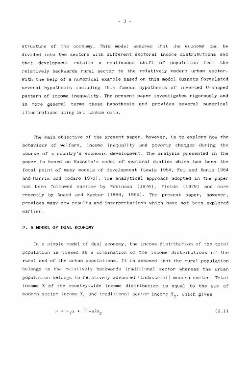
structure of the economy. This model assumes that the economy can be
divided into two sectors with different sectoral income distributions and
that development entails a continuous shift of population from the
relatively backwards rural sector to the relatively modern urban sector.
With the help of a numerical example based on this model Kuznets formulated
several hypothesis including this famous hypothesis of inverted U-shaped
pattern of income inequality. The present paper investigates rigorously and
in more general terms these hypothesis and provides several numerical
illustrations using Sri Lankan data.
The main objective of the present paper, however, is to explore how the
behaviour of welfare, income inequality and poverty changes during the
course of a country's economic development. The analysis presented in the
paper is based on Kuznets's model of sectoral dualism which has been the
focal point of many models of development (Lewis 1954, Fei and Ranis 1964
and Harris and Todaro 1970). The analytical approach adopted in the paper
has been followed earlier by Robinson (1976), Fields (1979) and more
recently by Anand and Kanbur (1984, 1985). The present paper, however,
provides many new results and interpretations which have not been explored
earlier.
2. A MODEL OF DUAL ECONOMY
In a simple model of dual economy, the income distribution of the total
population is viewed as a combination of the income distributions of the
rural and of the urban populations. It is assumed that the rural population
belongs to the relatively backwards traditional sector whereas the urban
population belongs to relatively advanced (industrial) modern sector. Total
income X of the country-wide income distribution is equal to the sum of
modern sector income X1 and traditional sector income X , which gives
H = H-^a + (l-a)n. (2.1)

- 4 -
where \i is the per capita income of the total population; n1 and (i2 are the
per capita incomes of the modern and traditional sectors, respectively, and
a is the proportion of population in the modern sector. This equation shows
that the per capita income in the economy is equal to the weighted sum of
the per capita incomes in the two sectors.
Development entails a monotonic shift of population from the
traditional sector to the modern sector. Differentiating (1) with respect
to a gives
which shows that if the per capita income in the modern sector (henceworth
to be called sector I) is higher than that in the traditional sector (to be
called sector II), which usually is the case, economic development leads to
monotonic increase in the per capita income of the total population. This
effect may be called the modern sector enlargement effect (Fields 1979).
It is obvious from (2.1) that the per capita income of the total
population is also affected by changes in the sectoral per capita incomes.
Differentiating (2.1) with respect to (i1 and \i2 gives
| * = a (2.3)
and
|^ = (1-a) (2.4)
respectively; which shows that the total per capita increases monotonically
with increases in the per capita incomes of either sectors. These may be
called enrichments effects caused by the changes in the income levels
within sectors (Fields 1979).
In order to analyze the effect of economic growth on welfare, it will
be necessary to consider a welfare measure which is not only sensitive to
the mean income but also to changes in the distribution of income. This can
be accomplished only if we allow for different sectoral income
distributions. Many of the development models of dual economy have assumed

- 5 -
that all persons within sectors have exactly the same income (or wages),
i.e., the inequality of income in the total population is only due to
intra-sectoral income differences (Lewis 1954, Fei and Ranis 1964, Harris
and Todaro 1970 and Fields 1979). The welfare analysis presented in the
next section allows for different intra-sectoral income distributions, in
the most general fashion.
3. WELFARE IN A DEVELOPING ECONOMY
This section explores how social welfare changes during the course of a
country's economic development. Before we discuss this issue, it will be
necessary to outline the concept of Lorenz curve which is widely used to
represent and analyze the size distributions of income and wealth. It is
defined as the relationship between the cumulative proportion of income
units and cumulative proportion of income received when units are arranged
in ascending order of their income.
The Lorenz curve is represented by a function L(p), which is
interpreted as the fraction of total income received by the lowest pth
fraction of income units. It satisfies the following conditions (Kakwani
1980):
(a) if p = 0, L(p) = 0
(b) if p = 1, L(p) = 1
(c) L'(p) ="^ >0 and L"(p) = ~j^j > 0 (3.1)
(d) L(p) < p
where income x of a unit is a random variable with probability density
function f(x) with mean \i and L'(p) and L"(p) are the first and second
derivatives of L(p) with respect to p, respectively.
The Lorenz curve has been used to compare inequality in income
distributions: for if the Lorenz curve for one distribution X lies anywhere
above that for another distribution Y, then the distribution X may be said
to be more equal than the distribution Y. However, the ranking provided by
the curve is only partial - when two Lorenz curves interest, neither
distribution can be said to be more equal than the other.

- 6 -
The Lorenz curve makes distributional judgement independently of the
size of income, which as Sen (1973) points out, "will make sense only if
the relative ordering of welfare levels of distributions were strictly
neutral to the operation of multiplying everybody's income by a given
number". This is rather an extreme requirement because social welfare
depends on both size and distribution of income.
Working independently on extensions of the Lorenz partial ordering
Shorrocks (1983) and Kakwani (1984) arrived at a criterion which would rank
any two distributions with different mean incomes. The new criterion given
by L(n, p) may be called the generalized Lorenz curve and is the product of
the mean income n and the Lorenz curve L(p). This criterion of ranking has
been justified from the welfare point of view in terms of several
alternative classes of social welfare functions. Thus, it can be said that
if the generalized Lorenz curve for distribution X lies everywhere above
that for another distribution Y, then distribution X is welfare superior to
distribution Y. This criterion may be used to judge between the
distributions without knowing the form of the welfare function except that
it is symmetric and quasi-concave in incomes.
The question to which this section is addressed is: What are the
conditions under which the modern sector enlargement and enrichment of
individual sectors will lead to higher welfare for the entire population?
Our main results are presented in the form of various propositions.
PROPOSITION 1. If the generalized Lorenz curve for the urban sector distribution lies everywhere above that for the rural sector distribution, the generalized Lorenz curve for the country-wide distribution will shift upwards at all points as migration takes place from the rural to urban sector.
1. Kakwani (1984) has used this criterion for international comparison of welfare using data from 72 countries.

The implication of this proposition is that if urban sector
distribution is welfare superior to the rural sector distribution, then the
migration from rural sector to urban sector will increase the welfare of 2
the country-wide distribution.
This proposition is proved below under the assumption that the
migration does not change the intra-sectoral distributions.
PROOF OF PROPOSITION 1
Suppose F1 (x) and F2 (x) are the probability distribution functions of
the urban and rural sector income distributions, respectively, then the
probability distribution function of the country-wide income distribution
is given by
F(x) = aF1 (x) + (l-a,F (x). (3.2)
where a is the proportion of population in the urban sector. Further,
suppose that L1 (p) and L2 (p) are the Lorenz functions for the urban and
rural sectors, respectively, the Lorenz function of the country-wide
distribution is then given by
|iL(p) = a(i1L1[F1(x)] + (l-a)n2L2[F2(x)] (3.3)
where p = F(x) can be assumed to be fixed.
Differentiating (3.2) and (3.3) with respect to a gives
3F (x) 3F (x) a ± + ( 1 - a ) — = F„(x) - F,(x) (3.4)
3a 3a 2 1
2. Anand and Kanbur (1984) have proved this proposition using the first and second order dominance conditions given in Hadar and Russell (1969).

and
iuUp) 3a
= n 1 L 1 [ F 1 ( x ) ] - n 2 L 2 [ F 2 ( x ) ]
3F (x) , 3F (x)
+ a , i L i [ F i ( x ) ] _ _ _ _ + ( 1 _ a ) | l 2 L 2 [ F 2 ( x ) ] _ _ _ , ( 3 . 5 ,
respectively, where use has been made of the assumption that p is fixed,
i.e., £=0.
Equation (3.1) implies that
x = |iL'(p) = H1L^[F1(x)] = K2L2 [F2(x)] (3.6i
which on using in (3.4) and (3.5) leads to
3|iL(p) H1L1[F1(x)] - ^2L2[F2(x)] + x[F2(x) - F^x] (3.7)
Applying the mean value theorem on the function L [ F ( x ) ] and using
(3.6), equation (3.7) simplifies to
3 ^ P ) = H1L1[F1(x)] - ^ [ F ^ x ) ] + [F2(x) - F1(x)]§ (3.8)
where
> 0 if F (x) - F (x) > 0
< 0 if F (x) - F (x)< 0
(3.9)
implying that [ F2 (x) - F1 (x)]§ > 0 always holds. It can be seen from (3.8)
that if n1 L1 [F1 (x)] - |i2 L2 [F1 (x)]>0, i.e., if the generalized Lorenz curve
for the urban sector distribution lies everywhere above that for the rural
sector distribution, the entire generalized Lorenz curve for the
country-wide distribution shifts upwards. This completes the proof of
proposition 1.
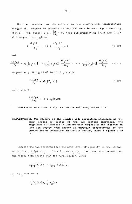
Next we consider how the welfare in the country-wide distribution
changes with respect to increase in sectoral mean incomes. Again assuming
that p = F(x) fixed, i.e., ^ = 0, then differentiating (3.2) and (3.3)
with respect to \i1 gives
3F (x) 3F (x) a + (l-a) = 0 (3.10)
and
, . , , , 3F (x) , 3F (x)
" ™ = a 4 [ F l ( x ) ] + ^ 1 L 1 [ F 1 ( X ) ] - ^ + (l-«)^2L2[F2(x)] - I S - (3.11)
respectively. Using (3.6) in (3.11), yields
9 ^ ( P ) = aL[F(x)] (3.12) 3y, ll 1
and similarly
^f^ = (1_a)L [F (x)] 3 \i2 2 2
These equations immediately lead to the following proposition.
PROPOSITION 2. The welfare of the country—wide population increases as the mean income of either of the two sectors increases. The magnitude of increase in welfare with respect to the increase in the ith sector mean income is directly proportional to the proportion of population in the ith sector, where i equals 1 or 2.
ense, i.e., L1 (p) = L2 (p) for all p and \i 1 > \i2 , i.e., the urban sector has
Suppose the two sectores have the same level of equality in the Lorenz
sense, i.e., L1 (p) = L2 (p) for all p and \i1 > \i2 i.e.,
the higher mean income than the rural sector. Since
H ^ t F ^ x ) ] = ^2L2[72U)\,
H > M2 must imply
L1'[F1(x)]<L2[F2(x)]

10
and if the Lorenz curves in the two sectors are identical, then F1 (x)<
F2 (x) must hold which implies
L^F^xJU L1[F2(x)]
It is reasonable to assume that a < (1-a), i.e., the proportion of
population in the urban sector is lower than that in the rural sector which
is a characteristic of developing countries, then
9|iL(p) 3(iL(p)
3yi 3 y 2
for all p must hold. This leads to the following proposition.
PROPOSITION 3. If the rural and urban sectors have the same Lorenz curve, the increase in the mean income of the rural sector will lead to greater increase in the country-wide welfare than the increase in the mean income of the urban sector.
It is easy to demonstrate that
H1L1[F1(x)] = xF1(x) - <f1(x) (3.13)
H2L2iF2(x)J = xF2(x) - <t>2(x) (3.14)
where
<f> (x) = / F (X)dX 0 x
<D (x) = / F (X)dX 0
Substituting (3.13) and (3.14) into (3.7) yields
3 ^ ( P ) = <t> (x) - <b(x) for all x (3.15;

- 11
which means that the larger the difference between the curves <o2> (x) and
O1 (x), the greater the shift in the country-wide generalized Lorenz curve
will be as a increases. Differentiating (3.6) with respect to n1 gives
3F (x) LitFi(x)]-^T=-l>
where x is assumed to be fixed. Using the Lorenz curve property (3.1) (c)
gives
L''[F,(X)] JIL r n u^U) '
where f1(x) being the density function of income distribution in sector I,
equation (3.14) yields
Since
3 ^
X
30.
(x)
' " l
i s
2 ( X
X
0
fixed
)
3F I :x)
l l dx
•J - /Xf.(X)dx = - L.[F. (x)] < 0. ^10 1 X X
will obviously be equal to zero. Thus, the difference between curves 02(x)
and <O1>(x) will widen for all x as \i1 increases {\i2 being fixed). This leads
to the following proposition.
PROPOSITION 4. If the generalized Lorenz curve for the urban sector is higher than that for the rural sector at all points, then the larger the per capita income differentials between the two sectors, the greater the increase in welfare will be, as the proportion of urban sector population increases.
Following the similar argument, one can easily arrive at the following
proposition
PROPOSITION 5. If the generalized Lorenz curve for the urban sector is higher than that for the rural sector at all points, then the smaller the intra-sectoral inequality differentials between the two sectors, the greater the increase in welfare will be, as the proportion of urban sector population increases.

- 12 -
4. INCOME INEQUALITY IN A DUAL ECONOMY
This section explores the behaviour of income inequality in a dual
economy which is characterized by the shift of population from the rural
sector to the urban sector.
Differentiating the lefthand side of (3.7) with respect to a and using
(3.3) yields
a L(p) _ iLiii^ 3a ~ \i2 [ L l ( F l ( x ) ) " L
2( F 2 ( x ) ) ] + J [ F 2 U ) " F 1 ( X ) ] ( 4 - 1 >
which on using the mean value theorem on the function L2 [F2 (x)] becomes
F (x) - F (x) ^ f 1 = J ^ W X ) ) - L2(Fl(x))] - [-? ^ ][^(x-§) - nx] (4.2)
H
where § as defined in (3.9) is given by
x - § = n2L^[F1(x) + 6(F2(x) - F1(x))] (4.3)
0 < 6 4 1; if F (x) - F (x) > 0, then §> 0, otherwise § is negative.
Assuming that the two sectors have the same Lorenz functions, then it
shown in
(4.3) implies
was shown in Section 3 that F2 (x) - F1 (x) > 0 for all x. Then equation
x - § > ^ L ^ F ^ x )
which on using (3.6) gives
'̂ 1 ~ ̂ 2 ^ ~ ̂ l5 ^ °"
Under these assumptions (4.2) can be written as
3L(D) F 2 ( X ) - F 1 U )
^ = - [-Z ^ — ] i(H - ,2)x - ̂ i - ax(p1 - ,2)]
Substituting a = 0 and 1, this equation gives
^ ^ < 0 for a = 0 3a
)UjLL > 0 for a = 1 3a

- 13 -
and
^ = 0 for
(Ux - H2)x - 1^5 a = -, r
(\i± - u2)x
which lies between 0 and 1. It means that as a increases, L(p) decreases
first, and then it increases, or in other words the relationship between
L(p) (for any fixed p) and a has a U-shaped form. This leads to the
following proposition.
PROPOSITION 6. If the rural and urban sectors have the same Lorenz curve, the relationship between inequality and development follows an inverted U-shaped pattern, with inequality first increasing and then decreasing.
It should be pointed out that Kuznets's hypothesis concerning the
inverted U-shaped curve was based on a simple numerical illustration.
Robertson(1976), however, provided a rigorous proof of the U-shaped
hypothesis but his analysis was based on one specific index of inequality -
the variance of the logarithm of income. Anand and Kanbur (1984) used the
general framework as adopted here and proved that at the start of the
development process, when a = 0,
£U£i <0. 8a
But this is an extreme situation when the entire population lives in the
rural sector or in other words the urban sector does not exist at all. The
above proposition provides a condition under which the income share of the
lowest 100 x p percent population (for all p) follows the inverted U-shaped
pattern of economic development.
The sufficient condition for the existence of inverted U-shaped curve
is that 3 > 0 as a approaches 1. It can be seen that as a approaches 1,
F1(x) approaches p and y approaches u1 . Substituting this in (4.2), it
immediately follows that
^ T a - = ^ 1 ^ - L 2 ( P > 1 + [F2(X) ^ W

in which the first term is negative and the second term positive. The net
effect of the two will be positive only if the difference in income
inequality between the two sectors is small. Thus, the existence of the
inverted U-shaped curve depends on the difference in the within sectors
inequalities - if with the economic development this difference enlarges,
it may be possible to have a situation when the inequality in the
country-wide distribution increases monotonically as a increases.
Assuming that the income inequality in the urban sector is higher than
that in the rural sector and the two sectors have the same per capita
income, obviously then, the generalized Lorenz curve for the rural sector
distribution will be higher than that for the urban sector distribution at
all points. Under these conditions, the difference <O2> (x) - <O1> (x) will be
negative for all x which from (3.15) implies that
V 3 ^ P < 0 for all p.
This leads to the following proposition.
PROPOSITION 7. If the income inequality in the urban sector is higher than that in the rural sector and the two sectors have the same per capita income, the inequality in the country-wide distribution increases monotonically as there is a shift in population from the rural sector to the urban sector.
Next we consider how the inequality in the country-wide distribution
changes with respect to increase in sectoral mean incomes. Differentiating
the lefthand side of (3.12) with respect to n1 and utilizing (3.3), gives
iiipi = aO^Ji^j _ j ( 4 4 )
o V 1 P 1 i d. d
and similarly
3L(p) _ a(l-a)m 3p.
y ^ - lL1(F1(x)) - L2(F2(x))] (4.5)
Suppose the two sectors have the same Lorenz function, then F2 ( x ) >
F1 (x) for all x which from (4.4) and (4.5) implies that
itifii < 0 and M£l > o 3Ui 3 y 2

- 15 -
which leads to the following proposition.
PROPOSITION 8. If the two sectors have the same inequality but the per capita income of the urban sector is higher than that of the rural sector, the enrichment of the urban (rural) sector increases (decreases) the inequality in the country—wide income distribution.
One of the implications of this proposition is that if the two sectors
have the different inequality in the Lorenz sense, it is not possible to
infer unambiguously that the increasing per capita income differential in
favour of the urban sector will necessarily lead to higher inequality in
the country-wide income distribution.
Applying the mean value theorem on L2[F2 (x)], (4.4) can be written as
i M p i = a U - a ) , ! , ^ ^ ^ _ L 2 ( F i ( x ) ) ] _
- a U' 2a ) [F2(x) - F1(x) ] (x-S)
where x-§ >0 (see equation 4.3). This derivative will be negative if F2 (x)>
F1 (x), otherwise its sign is indeterminant. This result immediately leads
to the following proposition.
PROPOSITION 9. If the urban sector has higher inequality than the rural sector, but F2 (x) > F1 (x), for all x, the enrichment of the urban (rural) sector increases (decreases) the inequality in the country-wide income distribution.
5. THE INEQUALITY-DEVELOPMENT RELATIONSHIP IN TERMS OF SINGLE INDICES OF
POVERTY
Whereas the Lorenz curve provides only a partial ranking of
distributions, measures of inequality have been devised to provide complete
ranking. This section explores the inequality-development relationship in a
dual economy in terms of several wellknown indices of income inequality.
- 16 -
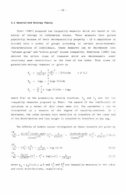
5.1 Generalized Entropy Family
Theil (1967) proposed two inequality measures which are based on the
notion of entropy in information theory. These measures have gained
popularity because of their decomposabiiity property - if a population is
divided into a number of groups according to certain socio-economic
characteristics of individuals, these measures can be decomposed into
"between group" and "within group" income inequality. Shorrocks (1980) has
derived the entire class of measures which are decomposable under
relatively weak restrictions on the form of the index. This class of
generalized entropy measures is given by
1 " * c
/[(-) - 1 ] f(x)dx c / 0,1 c(c-l) 0 |i
T = logn - / logx f(x)dx 0
T = — / x logx f(x)dx - logn '1 \i 0
where f(x) is the probability density function. T0 and T1 are the two
inequality measures proposed by Theil. The square of the coefficient of
variation is a member of this class when c=2. The parameter c can be
interpreted as a measure of the degree of equality-aversion. As c
decreases, the index becomes more sensitive to transfers at the lower end
of the distribution and less weight is attached to transfers at the top.
The effects of modern sector enlargement on these measures are given by
c _ ( 1 + § ) ° ( l + a § - a c § ) , 1 1 1 _ ( l + a § + c § - a c § ) , 2 1 , , .
3a ~ M s , c + l l c c ( c - l ) J . . _ . c + l [ c + c ( c - l ) M b - 1 J
( l + a § ) ( l + a § )
3T
(5.3)
1 and T 2
c and rural distributions, respectively
where u1 = u2(l+§),§ > 0 and T and T are inequality measures in the urban 1 2 c c

If we assume that the inequality in the urban sector distribution is
higher than that for the rural sector distribution, it can be seen from
(5.1) that
3T - ~ - > 0 for a = 0 3a
if (l+§) - (l+c§) > 0, which holds only if c > 1. As already pointed out,
Anand and Kanbur (1984) have proved that at the start of development
process when a = o, there is an unambiguous increase in inequality. This
result may not be true in the case of generalized entropy family when c < 1
(except when c = 0 and c = 1.0).
Assuming that the two sectors have the same inequality, it can be shown
that 3T 3T
< 0 for c > 1
3T
-£- Uo > ° 3T
-^ I n > ° 3a a=0
which lead to the following proposition.
and
and
and
3T c
3a
3To 3a
3T
3a
•a=l
>«=!
'« = !
< 0
< 0
< 0
PROPOSITION 10. If the rural and urban sector distributions have the same inequality and the urban sector has higher per capita income than the rural sector, the inequality measured by the entire family of generalized entropy measures (for c >1, c = 0 and 1.0) increases first and then decreases, as the population shifts from the rural to urban sectors.
Next, we consider the enrichment effects of modern and traditional
sectors on income inequality which are measured by the following
derivatives.
_ ^ c c o U - o ^ [ ( 1 + § )c-l ( T 1 + 1 ) _ (T2 + - T ^ - T T ) ] 3u» ,.. rtc
l c c(c-l) c c(c-l) p (1 +a §)
ca(l-a)(Ui2[(1+5)c-l ( T 1 + _ ! _ _ ) _ ( T2 + 1
/, ex- - c(c-l)' c c(c-l) H2 p(l+a§)
1 a(l-a) r _1 _ 2 /1 c \ l ~ = ., ' , T1 - T + log(l+§)| 3^! fi(l+a§) 1 1

^ = _ o u ^ U i i ! [ T i _ T l2
+ i o g ( i + § ) ly2 (i ( l+a§ ) 1 1
3 T0 a(l-a)§ 3pi M(1+§)
3 T0 a(l-a)§
The above equations immediately lead to the following proposition.
PROPOSITION 11. If the urban sector has higher inequality than the rural sector, the modern (traditional) sector enrichment leads to higher (lower) inequality (measured by the entire class of generalized entropy measures for c > 1, c = 0 and c = 1.0) in the country-wide distribution.
This proposition may not hold when c < 1 (except when c = 0).
5.2 Atkinson's measures
Atkinson (1970) proposed a family of inequality measures that are based
on the concept of "the equally distributed equivalent level of income".
These measures are derived from the social welfare function which is
utilitarian and every individual has exactly the same utility function.
Under the assumption that the individual utility function is nomothetic.
these measures are equal to
1
A(e) = 1 - -- [ / x 1 _ C f(x)dx] 1 _ £ , z * 1 ^ 0
= 1 - ̂ , e = 1
where g is the geometric mean of the distribution - and e is a measure of
the degree of inequality aversion - or the relative sensitivity to income
transfers at different income levels. As e rises, more and more weight is
attached to transfers at the lower end of the distribution and less weight
to transfers at the top. If e = 0, it reflects an inequality-neutral
attitude, in which the society does not care about the inequality at all.

- 19
The effects of modern sector enlargement on Atkinson's measures are
given by
3A(e) S[l-A(e)l [l-A(e)]E [(l+S)1"5 K,- K2] 3a (l + a§) ,. W n nl-c
(l-e)(l+a§)
3A(1) ^- = [l-A(l)] [-J^J - log(l+S) - logP1 + logP2]
K1 = (l-A^e))1 '
K2 = (1-A2^))1 €
1 2 A1 (e) and A2 (e) being the inequality measures in the urban and rural sector
distributions, respectively and
P1 = G1/n1 and P2 = G2/n2,
G1 and G2 being the geometric means of the urban and rural sectors,
respectively.
The following proposition follows from the above derivatives.
PROPOSITION 12. If the rural and urban sector distributions have the same inequality (measured by the entire class of Atkinson's measures) and urban sector has higher per capita than the rural sector, the inequality in the country-wide distribution follows an inverted U—shaped pattern as a increases during the course of a country's economic development.
The enrichment effects of modern and traditional sectors on inequality
are given by the following derivatives.
Iflil = a ( l - a ) [ l A ( e ) le [(1+|)E ;
U l li(l+a%)1 (l+§} £ * X
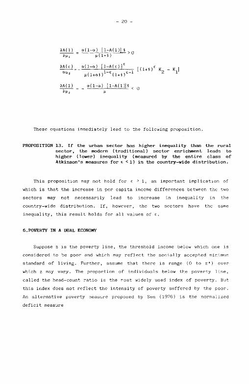
20 -
3 A ( 1 ) g ( l - g ) [ l - A ( l ) ] §
3 y , M ( 1 + S )
> M c ) c _ a ( l - a ) [ 1 - A ( £ ) ] e [ ( 1 + e _
ay j 2 /-, , , 1 - i : , , . , £ - 1 2 1 J
' H ( l + a § ) ( l + § )
3 A ( 1 ) = _ a ( l - a ) [ l - A ( l ) ] § <
3 p 2 (i 0
These equations immediately lead to the following proposition.
PROPOSITION 13. If the urban sector has higher inequality than the rural sector, the modern (traditional) sector enrichment leads to higher (lower) inequality (measured by the entire class of Atkinson's measures for e <1) in the country-wide distribution.
This proposition may not hold for e > 1, an important implication of
which is that the increase in per capita income differences between the two
sectors may not necessarily lead to increase in inequality in the
country-wide distribution. If, however, the two sectors have the same
inequality, this result holds for all values of e.
6.POVERTY IN A DUAL ECONOMY
Suppose z is the poverty line, the threshold income below which one is
considered to be poor and which may reflect the socially accepted minimum
standard of living. Further, assume that there is range (0 to z*) over
which z may vary. The proportion of individuals below the poverty line,
called the head-count ratio is the most widely used index of poverty. But
this index does not reflect the intensity of poverty suffered by the poor.
An alternative poverty measure proposed by Sen (1976) is the normalized
deficit measure

21
D = / t^-*i f(x)dx = F(z) (-̂ -) (6.1) 0 Z
where F(z) is the head-count ratio and \i* is the mean income of the poor.
This is a suitable measure of poverty if all the poor have exactly the same
income.
Since all the poor do not have exactly the same income several poverty
measures have been proposed in the literature which take into account the
inequality of income among the poor. A class of additively separable and
symmetric poverty measures is given by
z
G(P) = / P(x,z) f(x)dx (6.2) 0
where P(x,z) is a decreasing and differentiable function of x over (0,z)
and P(x,z) = 0 for x ~> z. Examples of members of this class are given in
Table 1 (Atkinson 1985)
TABLE 1: Class of Additively Separable Poverty measures
Normalized deficit D = / ( ) f(x)dx 0 Z
z Watt's (1968) measure W = /log (z/x) f(x)dx
o e
Foster, Green and Thorbecke (1984)
p = / (-5-5) f(x)dx, a > 1 a Q z
Clark, Hemming and Ulph (1981)
C = f / [ I - (f-)al f(x)dx a a Q
The following lemma has been proved by Atkinson (1985):
LEMMA. The following statements are equivalent
( a ) <t> ( z ) « <t> ( z ) f o r 0 < z-S ?,'
(b ) / P ( x , z ) f ( x ) d x < / P ( x , z ) f ( x ) d x f o r 0< z4 0 0

- 22 -
This lemma implies that if the generalized Lorenz curve for
distribution I is everywhere above that for distribution II, the
distribution I will have lower poverty than distribution II for all poverty
lines. This lemma in conjunction with (3.15) and Proposition 1 leads to
Proposition 14.
PROPOSITION 14. If the generalized Lorenz curve for the urban sector distribution is higher than that for the rural sector distribution at all points upto the income level z*, the country-wide poverty (measured by a class of additively separable poverty measures G(P)) decreases monotonically as the proportion of population in the urban sector increases.
The following propositions follow immediately from propositions 2,4
and 5.
PROPOSITION 15. The poverty in the country-wide population decreases as the mean income of either of the two sectors increases. The magnitude of decrease in poverty with respect to increase in the mean income of the ith sector is directly proportional to the proportion of population in the ith sector.
PROPOSITION 16. If the generalized Lorenz curve for the urban sector lies everywhere above that for the rural sector upto the income level z*, the larger the per capita income differential between the two sectors, the greater the decrease in poverty will be due to migration of population from the rural to the urban sector.
PROPOSITION 17. If the generalized Lorenz curve for the urban sector is higher than that for the rural sector, the smaller the intra-sectoral inequality differentials between the two sectors, the greater the decrease in poverty will be, as the proportion of urban sector population increases
A class of non-additive separable measures proposed by Kakwani (1980)
is given by
z k S(k) = i ~ - t /(z-x) [ 1 - | f ^ ] f(x)dx (6.3)
z 0 M Z J
which leads to Sen's (1976) well-known poverty measure when k = 1.0.
- 23 -
The following propositions follow immediately from the first order
dominance condition of Atkinson (1985).
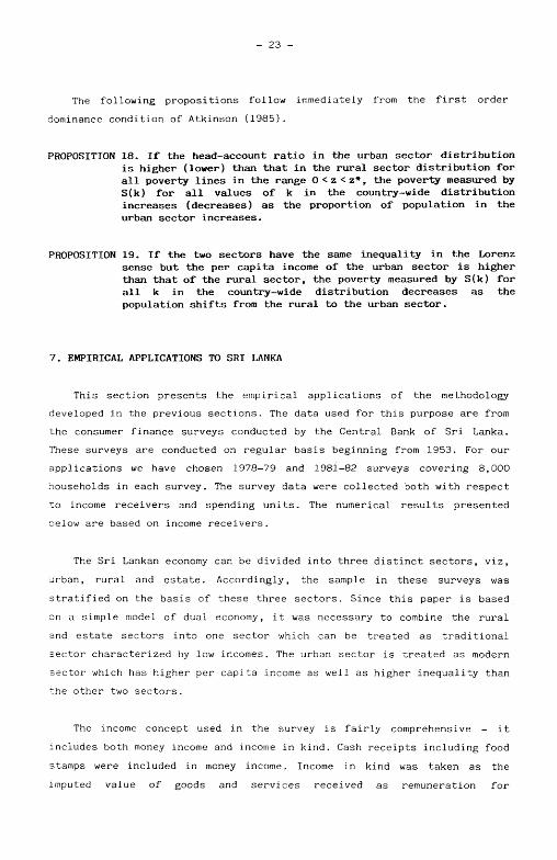
PROPOSITION 18. If the head-account ratio in the urban sector distribution is higher (lower) than that in the rural sector distribution for all poverty lines in the range 0 < z < z * , the poverty measured by S(k) for all values of k in the country-wide distribution increases (decreases) as the proportion of population in the urban sector increases.
PROPOSITION 19. If the two sectors have the same inequality in the Lorenz sense but the per capita income of the urban sector is higher than that of the rural sector, the poverty measured by S(k) for all k in the country-wide distribution decreases as the population shifts from the rural to the urban sector.
7. EMPIRICAL APPLICATIONS TO SRI LANKA
This section presents the empirical applications of the methodology
developed in the previous sections. The data used for this purpose are from
the consumer finance surveys conducted by the Central Bank of Sri Lanka.
These surveys are conducted on regular basis beginning from 1953. For our
applications we have chosen 1978-79 and 1981-82 surveys covering 8,000
households in each survey. The survey data were collected both with respect
to income receivers and spending units. The numerical results presented
oelow are based on income receivers.
The Sri Lankan economy can be divided into three distinct sectors, viz,
urban, rural and estate. Accordingly, the sample in these surveys was
stratified on the basis of these three sectors. Since this paper is based
on a simple model of dual economy, it was necessary to combine the rural
and estate sectors into one sector which can be treated as traditional
sector characterized by low incomes. The urban sector is treated as modern
sector which has higher per capita income as well as higher inequality than
the other two sectors.
The income concept used in the survey is fairly comprehensive - it
includes both money income and income in kind. Cash receipts including food
stamps were included in money income. Income in kind was taken as the
imputed value of goods and services received as remuneration for

- 24 -
employment, the imputed value of home production and transfer payments in
kind. The imputed value of owner occupied dwelling was treated as income in
kind.
Sri Lanka has been a unique example of a developing country whose
performance in terms of basic needs has been extremely impressive compared
to its income level. These impressive results were achieved as a result of
the social welfare policies followed by the successive governments since
World War II. Three major social policies followed were
(a) subsidised food
(b) free education system and
(c) a free health care service on a universal basis.
These policies involved massive expenditures which could only be maintained
by curtailing investment in the physical capital formation. As a result,
the growth slowed down and the country often ran into chronic balance of
payment problems.
The new goverment elected in 1977 changed the earlier welfare oriented
development strategy and introduced new economic policies which centered
around more growth and investment. One of the major policy changes was the
substitution of food subsidies by a means-tested food stamps programme. The
enormous savings made as a result of these changes were directed to
production and employment activities. Furthermore, the trade was liberated
and exchanged control was virtually withdrawn. This drastic change of
policies must have considerably affected the living standards of the
population. It is therefore important to analyze the data of 1978-79 and
1981-82 surveys in order to determine whether these growth oriented
policies led to increase or decrease in economic welfare in Sri Lanka.
In order to determine whether the welfare increases or decreases during
the course of economic development we compared the generalized Lorenz
curves for the urban and rural sectors which are displayed in Figures 1 and
2 for the years 1978-79 and 1981-82, respectively. It can be observed that
the generalized Lorenz curve for the urban sector distribution lies
everywhere above that for the rural sector distribution. Then according to
proposition 1, if the intra-sectoral distributions remain the same, the

- 25 -
migration from rural sector to urban sector will increase the welfare of
the country-wide distribution. Similarly, applying proposition 14, it can
be concluded that the country-wide poverty measured by a class of
additively separable poverty measures G(P) for any poverty line will
decrease monotonically as the proportion of population in the urban sector
increases provided, of course, the intra-sectoral distributions do not
change.
Figures 3 and 4 display the probability distribution functions for the
urban and rural sectors for the years 1978-79 and 1981-82, respectively. It
can be seen that the probability distribution function for the rural sector
lies everywhere above that for the urban sector. It means that for any
given poverty line z, the head-count ratio for the rural sector is always
higher than that for the urban sector. Then applying proposition 18, it can
be concluded that the country-wide poverty measured by the entire class of
poverty measures S(k) for all k decreases monotonically as the proportion
of population in the urban sector increases.
In order to determine how the welfare has changed during the period
1978-79 to 1981-82, it is necessary to convert the sectoral mean incomes
given at current prices to constant prices. For this purpose we used the
price index constructed by Edirisinghe (1985) which showed that prices
increased by 92 % during the period of three years (from 1978-79 to
1981-82). The mean incomes in each sector at current and constant prices
are given below.
Mean Income at Mean Income at
Sectors current prices at constant prices
1978-79 1981-82 1978-79 1981-82
Urban 827.51 1625 " 827.51 846.19
Rural/
Estate 557.86 988 557.86 514.63 All Island 616.85 1111 616.85 578.58

- 26 -
These figures show that the real income in the urban sector has
increased by 2.26 % in three years whereas in the rural/estate sector it
has decreased by about 7.75 %. As a result, the real income in the entire
population shows a decrease of about 6.20 %.
To compare the welfare levels over time, we plotted the generalized
Lorenz curves for the years 1978-79 and 1981-82 (see figures 5, 6 and 7).
It can be observed that the generalized Lorenz curve for the year 1978-79
lies everywhere above that for the year 1981-82 for whole island and the
rural/estate sector (figures 5 and 7), which demonstrates that the welfare
of the total population in Sri Lanka as well as that of the rural/estate 3
population has decreased unambiguously. In the case of urban sector
population, however, it is not possible to say unambiguously whether the
welfare has decreased or increased because the generalized Lorenz curves
for the two years (1978-79 and 1981-82) cross three times (at points where
p = .052, .097 and .988). In order to be able to make a definitive
statement concerning the welfare change in the urban sector it will be
necessary to compute single measures of welfare (see for instance Sen 1974
or Kakwani 1981).
Data on the distribution income were provided in the group form giving
(1) the number of income earners in each income range
(2) the total (for each range) of their incomes.
From these basic data we derived the data on p's and L(p)'s for each income
range. The following equation of the Lorenz curve was estimated by the
ordinary least-squares after applying the logarithmic transformation:
a B L(p) = p - ap (1-p)
3. When we say the welfare has decreased unambiguously, it means that this result is valid for a wide class of welfare functions(without specifying a welfare function).

- 27 -
where a, a and B are the parameters, and are assumed to be greater than
zero. The sufficient conditions for L(p) to be convex to the p axis are 0<
a 4 1 and 0 < R 4 1. This new functional form of the Lorenz curve was
introduced by Kakwani (1981) in connection with the estimation of a class
of welfare measures. This curve provided extremely good fit to the entire
range of income distribution data on Sri Lanka and was used to estimate the
various inequality measures.
A class of inequality measures which was estimated is the generalized
Gini index proposed by Kakwani (1986):
1 k-1 G(k) = 1 - k(k+l) / L(p)U-p) dp
0
which on substituting k = 1 leads to the well-known Gini index. The
parameter k is the measure of inequality aversion. As k rises, more and
more weight is attached to income transfers at the lower end of the
distribution and less weight to transfer at the top.
The estimated values of various inequality measures are presented in
Table 1. Kakwani's (1980) Lorenz measure given in the last row of the table
is given by
where I is the lenght of the Lorenz curve. This measure is sensitive to
income transfers at the lower end to income distribution. The conclusions
emerging from this table are summarized below.
The urban sector distribution is more unequal than the rural/estate
sector distribution in both years. This is evident from the estimates of
all the inequality measures. However, the gap between intra-sectoral
inequalities in the two sectors has widened considerably during the period
1978-79 to 1981-82. It means the inequality in the urban sector
distribution has increased considerably more than that in the rural/estate
sector. This is an important finding because it has implication for the
inverted U-shaped curve which will be discussed at a later stage.

- 28 -
The magnitude of the gap between the intra-sectoral inequalities in the
two sectors depends on the particular inequality measure. It is observed
that the gap becomes narrower as the parameter of inequality aversion
increases. For instance in the case of Atkinso's measures A(e ), e measures
the degree of inequality aversion - the larger the value of e , more and
more weight is attached to the lower end of the distribution than at the
middle and at the top. As e increases, the inequality gap between the two
sectors decreases from .017 to .012 in 1978-79 survey.
The income inequality has increased in both the sectors as well as in
all island during the period 1978-79 and 1981-82. This conclusion follows
from all inequality measures (except A(2.0) for rural/estate sector). The
income share of the first four quintile has decreased and that of the fifth
quintile increased during the three-year period.
Next we derived the behaviour of income inequality when the proportion
of population in the urban sector ( a ) varies from 0 to 1 keeping
intra-sectoral distributions unchanged. The results are presented in
figures 8 to 33. These diograms show how the indicators of inequality
change when the proportion of population in the modern sector increases.
Figures 8 to 18 display the inequality-development relationship based on
the income shares of each of the five quintiles for the years 1978-79 and
1981-82.
It can be seen that the income shares of the first two quintiles follow
the U-shaped curve - the share decreases first and then it increases. This
is observed in both 1978-79 and 1981-82 surveys. The share of the third
quintile follows the U-shaped curve for the year 1978-79 but in 1981-82, it
decreases monotonically. The share of the fourth quintile decreases
monotonically in both years as a increases from 0 to 1. The income share of
the 5th quintile, however, follows the inverted U-shaped curve - i.e., it
increases first and then decreases during the year 1978-79 but in 1981-82,
this share increases monotonically as a varies from 0 to 1. Although these
observations provide insight into the changes in the country-wide income

- 29 -
distribution at quintile points, they do no permit us to draw the
definitive conclusions regarding the behaviour of inequality-development
relationship. And, therefore, we turn to the remaining diograms (figures 19
to 33) which display the inequality-development relationships in terms of
single measures of income inequality.
It can be observed that most of the inequality measures follow the
inverted U-shaped pattern of development as hypothesized by Kuznets, i.e.,
with development, the inequality increases first and then decreases.
However, the turning points depend on the inequality measure used. Table 2
provides the turning points for various measures of inequality. Several
conclusions can be drawn from this table.
First, it is important to know where the turning point occurs - whether
at the early stages of development or at the late stage. It is apparent
that the inequality starts declining at a fairly late stage of development.
The minimum value of a is .556 and the maximum 1.0 and in almost all
developing countries the actual value of a is considerably less than .566.
It means that it will be considerably long time before the inequality
starts declining in the developing countries unless, of course, governments
in these countries follow the development strategy which redistributes
income in favour of low income earners.
Second, the different measures of inequality vary with respect to the
degree of inequality aversion. For instance, the generalized Gini index
G(k) becomes more and more sensitive to income transfers at the bottom end
of the distribution as k increases. It is interesting to note that the
turning point changes systematically with respect to the degree of
inequality aversion - the greater the degree of inequality aversion, the
smaller the turning point. This is an important finding - it implies that
with economic development poverty starts declining earlier than the income
inequality.
Third, in the case of some inequality measures, the turning point
occurs when a = l.0 which means that the inequality may never decline with
economic development implying that the Kuznets's inverted U-shaped curve
does not always exist.

- 30 -
Fourth, comparing 1978-79 and 1981-82 years it can be seen that turning
points have shifted forward for all inequality measures. Some of the
measures which followed the inverted U-shaped curve in 1978-79 show the
monotonic increase in income inequality. It means that intra-sectoral
distributions have changed (during the three-year period) such a way that
it will take much longer for income inequality in the country-wide
distribution to decrease (if at all) during the normal course of economic
development. It was observed earlier that the gap between the
intra-sectoral inequalities has considerably widened which has the effect
of shifting the turning forward. Thus, our emprical results are consistent
with the theory discussed in Section 4.
Next we discuss the empirical results on poverty in Sri Lanka which are
presented in Table 3. The poverty line was assumed to be Rs 200 per month
at 1978-79 prices. Since the analysis presented here is of illustrative
nature, it is unnecessary to discuss the controversy surrounding the
specification of the poverty line.
It can be observed that the poverty has increased in the rural/estate
sector and in the all Island during the period 1978-79 to 1981-82. This is
indicated by all the poverty measures. Since the generalized Lorenz curve
for 1978-79 lies everywhere above that for 1981-82 for the rural/estate
sector and for the all Island, then from Lemma 1 it follows that the
poverty measured by all decomposable poverty measures must increase for all
poverty lines. Thus, our empirical results are consistent with the
theoretically derived results.
Since the generalized Lorenz curves for the years 1978-79 and 1981-82
in the urban sector intersect, it is not possible to say, apriori, whether
the poverty in the urban sector has increased or decreased over time. It is
interesting to observe that the poverty measured by decomposable measures
which also include Normalized deficit decreases during the period from
1978-79 to 1981-82 whereas, that measured by head-count ratio and Kakwani's
class of measures (which also includes Sen's measure) increases during the
same period. Thus, the choice of poverty measures (whether decomposable or
non-decomposable) is important in determining the direction of change in
poverty.
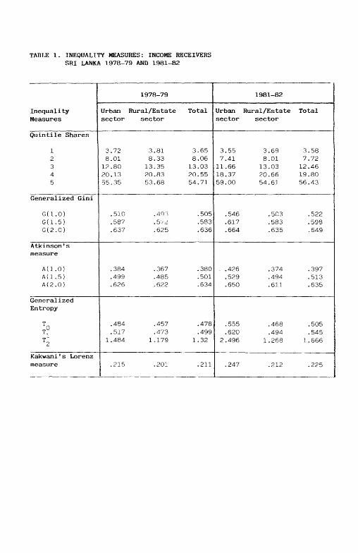
TABLE 1. INEQUALITY MEASURES: INCOME RECEIVERS SRI LANKA 1978-79 AND 1981-82
Inequality Measures
Quintile Shares
1 2 3 4 5
Generalized Gini
G(1.0) G{1.5) G(2.0)
Atkinson's measure
A(1.0) A(1.5) A(2.0)
Generalized Entropy
T
T2
Kakwani's Lorenz measure
1978-79
Urban Rural/Estate Total sector sector
3.72 3.81 3.65 8.01 8.33 8.06 12.80 13.35 13.03 20.13 20.83 20.55 55.35 53.68 54.71
.510 .493 .505
.587 .572 .583
.637 .625 .636
.384 .367 .380
.499 .485 .501
.626 .622 .634
.484 .457 .478
.517 .473 .499 1.484 1.179 1.32
.215 .201 .211
1981-82
Urban Rural/Estate Total sector sector
3.55 3.69 3.58 7.41 8.01 7.72 11.66 13.03 12.46 18.37 20.66 19.80 59.00 54.61 56.43
.546 .503 .522
.617 .583 .598
.664 .635 .649
. .426 .374 .397 .529 .494 .513 .650 .611 .635
.555 .468 .505
.620 .494 .545 2.496 1.268 1.666
.247 .212 .225

TABLE 2. TURNING POINTS FOR INVERTED U-SHAPED CURVE: SRI LANKA, INCOME RECEIVERS, 1978-79 to 1981-82
Inequality Measures
Income share of lowest
20 % population 40 % 60 % 80 %
Generalized Gini
G(1.0) G(1.5) G(2.0)
Atkinson's measure
A(1.0) A(1.5) A(2.0)
Generalized Entropy
Kakwani's Lorenz measure
1978-79 %
55.6 59.1 65.3 74.1
70.00 65.31 63.59
66.6 59.5 59.8
67.2 76.3 100.0
68.1
1981-82 %
62.3 71.2 84.3 100.0 (monot. incr.)
95.00 86.09 81.17
88.8 69.8 69.6
88.8 100.0 100.0
100.0

TABLE 3. POVERTY MEASURES: INCOME RECEIVERS SRI LANKA 1978-79 AND 1981-82
Poverty Measures
Head-count ratio
Normalized deficit
Kakwani *s Measures k equals
1.0 1.5 2.0
Decomposable poverty measures a equals
1.5 2.0 2.5 3.0
1978-79
Urban Rural/Estate Total sector sector
17.24 25.92 24.23
6.07 9.90 9.23
7.59 13.23 12.15 8.45 14.41 13.26 9.14 15.33 14.12
4.23 7.08 6.59 3.11 5.32 4.94 2.39 4.15 3.85 1.90 3.33 3.08
1981-82
Urban Rural/Estate Total sector sector
17.83 29.78 27.26
6.06 11.85 10.48
7.78 15.71 13.91 8.68 16.96 15.10 9.41 17.93 16.03
4.19 8.53 7.47 3.07 6.42 5.60 2.35 5.00 4.34 1.86 3.99 3.46

REFERENCES
Adelman, I and C.T. Morris, 1973, Economic Growth and Social Equity in Developing Countries, Stanford University Press, Stanford, California.
Ahluwalia, M.S., 1974, "Income Inequality: Some Dimensions of the Problems", in H. Chenery and others, Redistribution with Growth, Oxford University Press, London.
Ahluwalia, M.S., 1976, "Inequality, Poverty and Development", Journal of Development Economics, Vol.3, pp 307-342.
Anand, Sudhir and S.M. Ravi Kanbur, 1984, "The Kuznets Press and the Inequality-Development Relationship", Discussion Paper Series No.249, Department of Economics, University of Essex.
Anand, Sudhir and S.M. Ravi Kanbur, 1985, "Poverty under the Kuznets Process", The Economic Journal, pp 42-50.
Atkinson, A.B., 1970, "On the Measurement of Inequality", Journal of Economic Theory, Vol.2, pp 244-263.
Atkinson, A.B., 1985, "On Measurement of Poverty", Discussion paper No.90, Economic and Social Research Council Programme.
Bacha, E.L., 1977, "The Kuznets Curve and Beyond", Development Research Center, World Bank.
Chenery, H.B. and M. Syrquin, 1975, "Patterns of Development. 1950-1970", Oxford University Press, New York.
Clark, S.R., R. hemming and D. Ulph, 1981, "On Indices for Poverty Measurement", Economic Journal, Vol.91, pp 515-526.
Edirisinghe, Neville, 1985, "The food Stamp Progam in Sri Lanka: Costs. Benefits and Policy Options", International Food Policy Researcn Institute, 1776 Massachusetts Avenue, N.W., Washington D.C.
Fei, J.C.H. and G.Ranis, 1964, Development of the Labour Surplus Economy: Theory and Policy, Homewood.
Fields, G.S., 1979, "A Welfare Economic Analysis of Growth and Distribution in the Dual Economy", Quarterly Journal of Economics.
Foster, J.E., J. Greer and E. Thorbecke, 1984, "A Class of Decomposable Poverty Measures", Econometrica, Vol.52, pp 761-776.
Hadar, J. and W.R. Russell, 1969, "Rules for Ordering Uncertain Prospects", American Economic Review, Vol.59, pp 25-34.

Harris, J.R. and M. Todaro, 1970, "Migration, Unemployment and Development: A Two Sector Analysis", American Economic Review, March, Vol.60, pp 126-143.
Kakwani, N.C., 1980, "On a Class of Poverty Measures", Econometrica, Vol.48, No.2, March, pp 437-446.
Kakwani, N.C., 1980, Income Inequality and Poverty: Methods of Estimation and Policy Applications, Oxford University Press, New York.
Kakwani, N.C., 1981, "Welfare Measures: An International Comparison", Journal of Development Economics, Vol.8, pp 21-45.
Kakwani, N.C., 1984, "Welfare Ranking of Income Distributions", Advances in Econometrics, Vol.3, pp 191-213.
Kakwani, N.C., 1986, Analyzing Redistribution Policies: A Study Using Australian Data, Cambridge University Press, New York.
Kravis, I.B., 1960, "Internationa] Differences in the Distribution of Income", Review of Economics and Statistics, Vol.42, pp 408-416.
Kuznets, S., 1955, "Economic Growth and Income Inequality", American Economic Review, Vol.45, March, pp 1-28.
Lewis, W.A., 1954, "Economic Development with Unlimited Supplies of Labour", Manchester School of Economic and Social Studies, Vol.22, May, pp 139-191.
Oshima, H.T., 1962, "The International Comparison of Size Distribution of Family Incomes with Special Reference to Asia", Review of Economics and Statistics, Vol.44, pp 439-445.
Paukert, F., 1973, "Income Distribution at Different Levels of Development: A Survey of Evidence", International Labour Review, Vol.108, No.2-3.
Robinson, Sherman, 1976, "A Note on the U-Hypothesis Relating Income Inequality and Economic Development", The American Economic Review, Vol.66, June, pp 437-440.
Saith, Ashwani, 1983, "Development and Distribution: A Critique of the Cross-Country U-Hypothesis", Journal of Development Economics, Vol.13, pp 367-368.
Sen, Amartya, 1973, On Economic Inequality, Oxford: Clarendon Press.
Sen, Amartya, 1976, "Poverty: An Ordinal Approach to Measurement", Econometrica, Vol.44, No.2, March, pp 219-231.

Shorrocks, Anthony F., 1980, "The Class of Additively Decomposable Inequality Measures", Econometrica, Vol.48, No.3, pp 613-626.
Shorrocks, Anthony F., 1983, "Ranking Income Distributions", Economica.
Theil, H., 1967, Economics and Information Theory, Amsterdam: North-Holland.
Watts, H.W., 1968, "An Economic Definition of Poverty" in D-P. Moynihan (ed.), On Understanding Poverty, Basic Books: New York, pp 316-329.

Figure 1. GENERALIZED LORENZ CURVES FOR URBAN AND RURAL SECTORS: INCOME RECIPIENT UNITS IN SRI LANKA 1978-1979

Figure 2. GENERALIZED LORENZ CURVES FOR URBAN AND RURAL SECTORS: INCOME RECIPIENT UNITS I SRI LANKA 1981-1982

Figure 3. PROBABILITY DISTRIBUTION FUNCTION FOR URBAN AND RURAL SECTORS: INCOME RECIPIENT UNITS IN SRI LANKA 1978-1979

Figure 4. PROBABILITY DISTRIBUTION FUNCTION FOR URBAN AND RURAL SECTORS: INCOME RECIPIENT UNITS IN SRI LANKA 1981-1982

FIGURE 5. PLOT OF GENERALIZED LORENZ CURVES FOR TWO YEARS: 1978-79 AND 1981-82, SRI LANKA, ALL ISLAND

FIGURE 6. PLOT OF GENERALIZED LORENZ CURVE FOR TWO YEARS: 1978-79 AND 1981-82, SRI LANKA, URBAN SECTOR

FIGURE 7. PLOT OF GENERALIZED LORENZ CURVES FOR TWO YEARS: 1978-79 AND 1981-82, SRI LANKA, RURAL/ESTATE SECTOR

FIGURE 8.INEQUALITY-DEVELOPMENT RELATIONSHIP BASED ON THE INCOME-SHARE OF THE POOREST 20 % POPULATION: SRI LANKA, 1978-79

FIGURE 9.INEQUALITY-DEVELOPMENT RELATIONSHIP BASED ON THE INCOME-SHARE OF THE POOREST 20 % POPULATION: SRI LANKA, 1981-82

FIGURE 10. INEQUALITY-DEVELOPMENT RELATIONSHIP BASED ON THE INCOME-SHARE OF THE 2nd QUINTILE: SRI LANKA, 1978-79

FIGURE 11 INEQUALITY-DEVELOPMENT RELATIONSHIP BASED ON THE INCOME-SHARE OF THE 2nd QUINTILE: SRI LANKA, 1981-82

FIGURE 12 INEQUALITY-DEVELOPMENT RELATIONSHIP BASED ON THE INCOME-SHARE OF THE 3rd QUINTILE: SRI LANKA, 1978-79
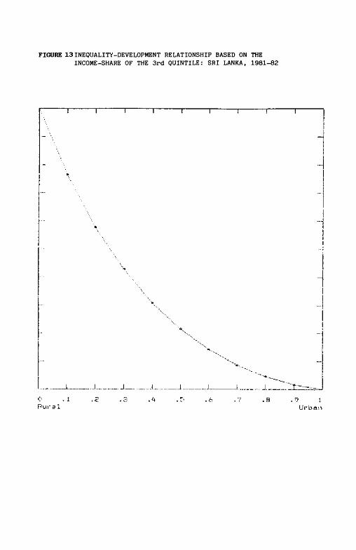
FIGURE 13 INEQUALITY-DEVELOPMENT RELATIONSHIP BASED ON THE INCOME-SHARE OF THE 3rd QUINTILE: SRI LANKA, 1981-82

FIGURE 14 INEQUALITY-DEVELOPMENT RELATIONSHIP BASED ON THE INCOME-SHARE OF THE 4th QUINTILE: SRI LANKA, 1978-79
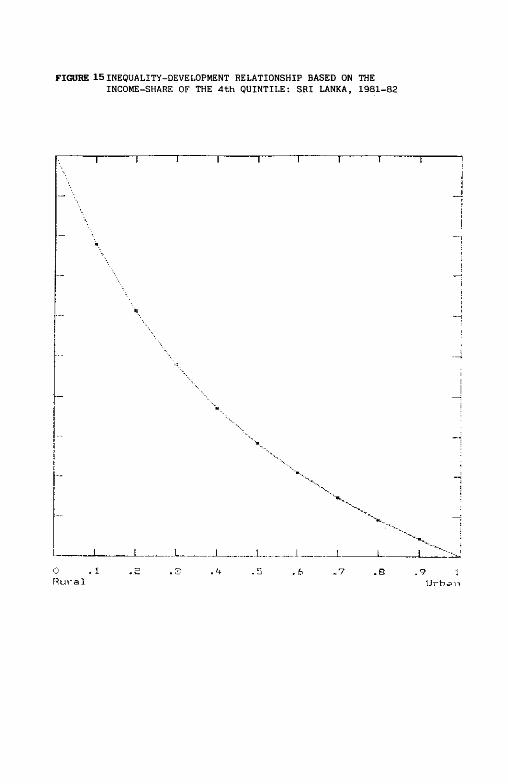
FIGURE 15 INEQUALITY-DEVELOPMENT RELATIONSHIP BASED ON THE INCOME-SHARE OF THE 4th QUINTILE: SRI LANKA, 1981-82

FIGURE 16 INEQUALITY-DEVELOPMENT RELATIONSHIP BASED ON THE INCOME-SHARE OF THE 5th QUINTILE: SRI LANKA, 1978-79

FIGURE 17 INEQUALITY-DEVELOPMENT RELATIONSHIP BASED ON INCOME-SHARE OF THE 5th QUINTILE: SRI LANKA 1981-82

FIGURE 18 INEQUALITY-DEVELOPMENT RELATIONSHIP BASED ON ATKINSON'S MEASURE FOR e = 1.0, SRI LANKA, 1978-79
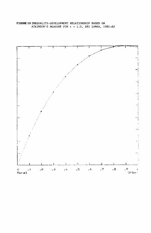
FIGURE 19 INEQUALITY-DEVELOPMENT RELATIONSHIP BASED ON ATKINSON'S MEASURE FOR e = 1.0, SRI LANKA, 1981-82
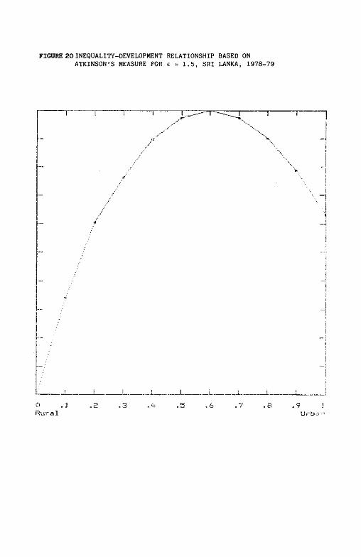
FIGURE 20 INEQUALITY-DEVELOPMENT RELATIONSHIP BASED ON ATKINSON'S MEASURE FOR e = 1.5, SRI LANKA, 1978-79

FIGURE 21 INEQUALITY-DEVELOPMENT RELATIONSHIP BASED ON ATKINSON'S MEASURE FOR e = 1.5, SRI LANKA, 1981-82

FIGURE 22 INEQUALITY-DEVELOPMENT RELATIONSHIP BASED ON ATKINSON'S MEASURE FOR e = 2.0, SRI LANKA, 1978-79

FIGURE 23 INEQUALITY-DEVELOPMENT RELATIONSHIP BASED ON ATKINSON'S MEASURE FOR e = 2.0, SRI LANKA, 1981-82
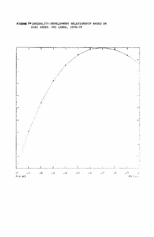
FIGURE 24 INEQUALITY-DEVELOPMENT RELATIONSHIP BASED ON GINI INDEX: SRI LANKA, 1978-79

FIGURE 25 INEQUALITY-DEVELOPMENT RELATIONSHIP BASED ON GINI INDEX: SRI LANKA, 1981-82

FIGURE 26 INEQUALITY-DEVELOPMENT RELATIONSHIP BASED ON GENERALIZED GINI INDEX FOR k = 1.5, SRI LANKA, 1978-79
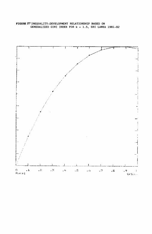
FIGURE 27 INEQUALITY-DEVELOPMENT RELATIONSHIP BASED ON GENERALIZED GINI INDEX FOR k = 1.5, SRI LANKA 1981-82

FIGURE 28 INEQUALITY-DEVELOPMENT RELATIONSHIP BASED ON GENERALIZED GINI INDEX FOR k = 2, SRI LANKA, 1978-79

FIGURE 29 INEQUALITY-DEVELOPMENT RELATIONSHIP BASED ON GENERALIZED GINI INDEX FOR k = 2, SRI LANKA, 1981-82

FIGURE 30 INEQUALITY-DEVELOPMENT RELATIONSHIP BASED ON GENERALIZED ENTROPY MEASURE T0 : SRI LANKA, 1978-79

FIGURE 31 INEQUALITY-DEVELOPMENT RELATIONSHIP BASED ON GENERALIZED ENTROPY MEASURE T0 : SRI LANKA, 1981-82

FIGURE 32. INEQUALITY-DEVELOPMENT RELATIONSHIP BASED ON GENERALIZED ENTROPY MEASURE, T1 : SRI LANKA, 1978-79

FIGURE 33. INEQUALITY-DEVELOPMENT RELATIONSHIP BASED ON GENERALIZED ENTROPY MEASURE, T1 : SRI LANKA, 1981-82