incompressible flow computations based on … · incompressible flow computations based on the...

Comparers & Srrucrures Vol. 35. No. 4, pp. 445-472, 1990

Printed in Great Britain.

00457949/90 $3.00 + 0.00 Pergamon Press plc

INCOMPRESSIBLE FLOW COMPUTATIONS BASED ON THE VORTICITY-STREAM FUNCTION

AND VELOCITY-PRESSURE FORMULATIONS

T. E. TEZDUYAR, J. LIOU and D. K. GANJOO

Department of Aerospace Engineering and Mechanics and Minnesota Supercomputer Institute, University of Minnesota, Minneapolis, MN 55455, U.S.A.

Abstract-Finite element procedures and computations based on the velocity-pressure and vorticity- stream function formulations of incompressible flows are presented. Two new multi-step velocity-pressure formulations are proposed and are compared with the vorticity-stream function and one-step formulations. The example problems chosen are the standing vortex problem and flow past a circular cylinder. Benchmark quality computations are performed for the cylinder problem. The numerical results indicate that the vorticity-stream function formulation and one of the two new multi-step formulations involve much less numerical dissipation than the one-step formulation.

1. INTRODUCTION

In this paper we focus on the finite element solution techniques and benchmark computations based on the velocity-pressure and vorticity-stream function formulations of the incompressible Navier-Stokes equations. We are interested in both steady-state and time-dependent solutions, including those which are periodic in time.

An important point to remember about the vorticity-stream function formulation is that the continuity equation is satisfied automatically and the pressure does not directly appear as an unknown in the formulation. The methods we have developed for the vorticity-stream function formulation so far are restricted to two-dimensional flows. These methods are applicable to both viscous and inviscid flows including problems with multiply-connected domains

[I, 21. The solution techniques presented here for the

velocity-pressure formulation can be extended to three-dimensional problems. We propose two new multi-step methods and compare them with the vorticity-stream function formulation and with the one-step method developed by Brooks and Hughes [3]. In all these formulations we use the streamline- upwind/Petrov-Galerkin (SUPG) method [l-3] to prevent the spurious oscillations that might appear in the presence of strong convective terms. In the velocity-pressure formulations presented in this paper we employ piecewise bilinear functions for the velocity and piecewise constant functions for the pressure.

In the one-step formulation the velocity is treated explicitly in the momentum equation. In the context of an incremental solution procedure, by eliminating the adceleration increment between the discrete momentum and continuity equations one can obtain an equation for the pressure increment alone; this equation for the pressure increment can be viewed as

a discrete Poisson equation. Several iterations can be performed to compensate for the explicit treatment of the velocity. In the one-step formulation the SUPG supplement to the weighting function is applied to all the terms in the momentum equation. If the pressure is interpolated with piecewise constant functions then the coefficient matrix of the equation for the pressure increment is symmetric and positive; however, if higher-order functions are used to interpolate the pressure, then, because of the SUPG supplement term, we cannot expect this coefficient matrix to be symmetric.

Our three-step T3 formulation starts out with a splitting scheme in which the pressure and the viscous terms are treated implicitly in the first and third steps while the convective terms are treated implicitly in the second step. This type of splitting is a special case of the kind found in the e-scheme [4]. We use the SUPG supplement only in the second step. In the current implementation the first and second steps are solved by a procedure which is very similar to the one described for the one-step formulation. However in this case the coefficient matrix of the equation for the pressure increment is symmetric and positive, independent of the kind of functions used to interpolate the pressure.

Our second multi-step scheme, which we will call the T6 formulation, is an extension of the T3 scheme. In this formulation the second step is subdivided into two sub-steps to isolate the convective terms. This way the SUPG supplement is applied only to the sub-step involving the convective terms. The first and third steps can also be subdivided into sub-steps if the ‘Stokes sub-step’ needs to be treated in a special way. In either way, again, the coefficient matrix of the equation for the pressure increment is symmetric and positive.

We consider two numerical examples: the standing vortex problem [5] and flow past a circular cylinder. The purpose of the standing vortex problem is to

446 T. E. TEZDUYAR er al.

obtain an indication of how much numerical dissipation is involved in a numerical solution technique. The second problem has been studied by several researchers in the past (see, for example, [6]); we perform benchmark quality computations for this problem and compare the results obtained with the various formulations described in this paper.

2. VELOCITY-PRESSURE AND VORTICITYSTREAM FUNCTION FORMULATIONS

Let R and (0, T) denote the spatial and temporal domains with x and t representing the coordinates associated with R and (0, T). The boundary r of the domain R may involve several internal boundaries. We consider the following velocity-pressure formulation of the incompressible Navier-Stokes equations:

P(L1u/at +u.Vu)--V.a=O on Rx (0,T) (1)

V.u=O on Rx (0,T) (2)

where p and u are the density and velocity and o is the stress tensor given as

d = -pI + 2/&u) (3)

with

c(u) = (Vu + (Vu)?)/2. (4)

Here p and p represent the pressure and viscosity while I denotes the identity tensor. Both the Dirichlet- and Neumann-type boundary conditions are taken into account as shown below

u=g on r,,

n.a=h on Tr,

(5)

(6)

where r, and f,, are mutually complementary subsets of l-.

In two-dimensional space the vorticity-stream function formulation of the incompressible Navier- Stokes equations consists of a convection-diffusion equation for the vorticity and a Poisson equation for the stream function

p(&o/& +u.Vo)--pVzw =0 on Rx (0,T) (7)

V** + 0 = 0 on R x (0, T), (8)

with the stream function and vorticity defined as

u = {a$&, -a$/%} (9)

w = aU21aX, - au, lax,. (10)

The components of the velocity vector u in the directions denoted by the unit vectors n and r can be expressed as

u,=n.u= -a+iaz (11)

U, = ‘5.~ = all/Ian. (12)

In this paper the unit vectors n and r represent the normal and tangential directions at a boundary. We consider various types of boundary conditions.

At an (external or internal) no-slip boundary the normal component of the velocity must be specified:

u, = (&)A ; (13)

for viscous flows the tangential component must also be specified:

u, = (u,),. (14)

Here (u,), and (u,), are given functions on the kth segment of the boundary F. The equivalent boundary conditions for the vorticity-stream function formulation are shown below

a+/ar = -(a,), (15)

ati /an = (u, )k. (16)

It should be noted that this form of the boundary conditions can also be used to impose a given velocity field at an upstream boundary.

Remark 1

In the vorticity-stream function formulation, for internal boundaries, in general, additional equations are needed to determine the unknown values of the stream function at such boundaries. These additional equations can be derived by integrating the equation of motion in the velocity-pressure form along each internal boundary. The interested reader can refer to [1,2] for more details on this issue.

Along a symmetry line we impose the following conditions:

11, = 0 (17)

fi au, jatt = 0. (18)

For the vorticity-stream function formulation the equivalent boundary conditions are

a*ja7 = 0 (19)

w =o. (20)

For inviscid flows the conditions (18) and (20) vanish. At a downstream boundary for the velocity-

pressure formulation we impose the traction-free conditions by specifying the stress vector to be zero, i.e.

a,=n.a.n=O (21)

a,=n.a.r=O. (22)

Incompressible flow computations 447

For the vorticity-stream function formulation, at a downstream boundary we set the normal derivative of both the vorticity and the stream function to zero. Of course this is not equivalent to the traction-free conditions of the velocity-pressure formulation, but we expect for at least hope) that if the do~stream boundary is far enough the differences will not be so significant.

To compute the pressure on the surface of an obstacfe (i-e_ an internal ~undary) in the flow field, we consider the following alternative form of the momentum equation (1)

-uxo+(I(fp)VpfvVxa,=O, (23)

where v is the kinematic viscosity. By taking the projection of the two-dimensiona version of this equation in the direction of z, we obtain

a4at + (iiz)a(ttf + ufyaz

- q$fJ + ~~/~~~/~~ + ~~~/~n = 0. (24)

We will assume that at all internal surfaces the normal component of the velocity is zero, i.e. u, = 0. For viscous fiows, by further assuming that au,/& = 0 and by integrating eqn (24) from a reference point I, to the point of interest 72, we obtain

For inviscid flows we integrate eqn (24) only with the ass~ption that u,= 0 _ _

Combining eqn (26) with eqn (12) we

1.2

obtain

(27)

Equations (25) and (27) can be used to compute the pressure at any point on an internal surface relative to a reference paint on that surface. The normal and tangential components of the stress vector can be calculated using the fo~Iowing expressions:

a,= -p (28)

a, = -_i.lcu. (29)

3. SPATIAL AND TEMPORAL DISCRETIZATKJNS

Let E denote the set of elements resulting from the finite element discretization of the computational

domain $2 into subdomains R”, e = 1,2,. . . , n,,, where n,, is the number of elements. We associate to E the finite dimensional spaces N’” and Ho’, where Hlh and Hoh represent the piecewise bilinear and piecewise constant finite element function spaces. The trial and test function spaces are given as

S/: = {uhIuhE(Hlh)n,: uh =gh on mf (30)

vl: = ~~~1~~~~‘~~~~ Wh& on r,) (311

S; =: Vi = {qhlqhE Hoh}, (32)

where n, is the number of space dimensions. The on~-ste~~~~~~ff~~o~ employed in this work is

essentially the same as the one used in [3]: find uh E S: and ph E Si such that

Here Sk is the SUPG suppiement to the weighting function dl. We use the fotfowing expression for $:

with

6k = zC*,(h/2)(uk/(l Uk Il)*Vw (34)

(35)

where the element level. Reynolds number is defined as

Re = II uk II h/(2v). (36)

The ‘element length’ h is commuted by using the expression [7j

where N, is the basis function associated with node a and ncn is the number of element nodes. For the ‘algorithmic Courant number” C,, we can use either C,, = 1 or C, = C,,, where C,, = 11 nh If Ar/h is the element level Courant number and At is the time step. Details on the selection of Czr can be found in [7].

The semi-discrete equations corresponding to eqn (33) can be written as follows:

tia+R(v)+litv-Gp=E

GTv = E,

(38)

(3%

448 T. E. TEZDLJYAR et al.

where v is the vector of unknown nodal values of uh, a is the time derivative of v, and p is the vector of nodal values of ph. Equations (38) and (39) are semi- d&zete ver_sions of eqns (1) and (2). The matrices A, N, K, and G are derived, respectively, from the time- dependent, convective, viscous, and pressure terms. The vector @ is due to the Dirichlet- and Neumann- type boundary conditions [i.e. the g and /I terms in eqns (5) and (6)], whereas the vector E is due to the Dirichlet-type boundary condition. All the arrays with a superposed tilde can be decomposed into their Galerkin and Petrov-Galerkin parts

ti=M+~, (40)

fi=N+~, (41)

ii=K+~~ (42)

c=G+Gd (43)

F=F+F,, (44)

where the subscript 6 identifies the Petrov-Galerkin contribution.

Remark 2

When the pressure is interpolated by a piecewise constant function space the matrix G, vanishes; however, in general, this does not have to be the case.

The predictor/multi-corrector time integration algorithm used for solving eqns (38) and (39) is based on the following incremental formulation:

where

M*Aa - CAp = R

G’Aa = Q,

(45)

(46)

R=p-(lha+R(v)+gv-?;p) (47)

Q = (l/(aAr))(E - G’v) (48)

. M*=lh+ccAt(dA/av+ii). (49)

The parameter LY controls the stability and accuracy of the time integration algorithm. By eliminating Aa between eqns (45) and (46) we obtain an equation for Ap alone

(Gr(M*)-‘z;)Ap = Q - GT(M*)-‘R. (50)

Once eqn (50) is solved for Ap, As can be computed by using the following expression:

Remark 3

If M* is approximated with a diagonal version of eqn (49) then the solution of eqns (50) and (51) becomes more feasible and economical. We can achieve this by approximating M* with M,,,,, where MLUMP is the lumped version of the mass matrix M. Further- more, if a piecewise constant function space is used to interpolate the pressure (see Remark 2) then the coefficient matrix of Ap in eqn (50) becomes symmetric and positive. This would facilitate the utilization of symmetric (direct or iterative) matrix solvers. For example, it might be possible, with a suitable precon- ditioning matrix, to use the conjugate gradient method [8] to solve eqn (50).

We now propose a new formulation based on the three-step Q-scheme [4]; we will formulation as the T3 formulation:

refer to this

find u~+~E(S~),+~ and P~+~ES~ such that

r

J wh.p((u;+s-u;)/(OAt)+u;~Vu;)dR cl

+ s

c(wh):4+@dCl+ qhV.uI:+8dR R s n

= s wh.h;+@, Vwhs Vi, VqhE V;; (52) rl

find ~j:+,_~e(S~)~+,_~ such that

+4+,-D. Vul:+,_,)dR+ s

e(wh):$n+odR R

+uj:+,-0 .Vuj:+,_,)-V.aj:+,]dR

= wh.h;+o dr, Vwhe V:; (53)

find II;+, E (Si),,, and pi+, E Si such that

s +P((uhn+ I - 4+ 1 -oHeAt) n

+uL-0 .Vu:+,_,)dfl

+ s e(wh):oj:+,dR+ qhV.u;+, dR n

= s wh.h;+,, VW~E Vi, Vqhc Vi. (54) rh

Remark 4

(51) The SUPG sunnlement is limited onlv to steo (53). . ~ Aa = (M*)-‘R + (M*)-‘GAP.


Remark 5

Steps (52) and (54) can be solved by a procedure which is a special case of the one described by eqns (38)-(51). In this case, however, G6 vanishes independent of the type of function space used for the pressure (see Remark 2). Therefore if M* is approximated by ML,,, then the coefficient matrix of Ap in eqn (50) becomes symmetric and positive for all combinations of the interpolation functions used for the velocity and pressure.

Remark 6

It is possible to use equal-order of interpolation functions for the velocity and pressure by adding a Petrov-Galerkin supplement to steps (52) and (54). Our preliminary computations based on such formulations exhibited no convergence difficulties and resulted in reasonable solutions for the test problem of flow past a circular cylinder at Reynolds number 100 (see [9]).

Remark 7

Equation (53) is the nonlinear step in this formulation; it can be solved by a multi-iteration implicit or explicit method. These two choices give us the implicit and explicit verisons of the T3 scheme.

As an extension of the T3 scheme, we propose another formulation which we will refer to as the T6 formulation :

find ii+,r~(S:),+, such that

+ II;. Vu:) dR

=o. VWhE vi; (55)

find II!,,, E (Si),,,, and pi+0 E Si such that

+ s c(wh):c;+OdCl + I

q*V.ul:+“dn n n

= s wh.h:+,, VW~E V!& VqhE Vi; I‘*

find iii,, _,,e(Si),,+ ,__” such that

s w”.P(@~:+, -,, - u;+nM - 3.9) AtI) do 0

+ s ~(w~):uj:+~dR n

= s

w”.h;+,,dl-, V why Vi; r*

(56)

(57)

find u~+,_~E(S&+,_~ such that

+u:+,-e .VuL-,)dQ

+4+,-o .V~f:+,_~)]dR=o, VW”E Vi; (58)

find ii + , E (Si),, + , such that

I w*.&+, -ul:+,-,)/@A0

n

+uf:+,-0 .Vuj:+,_,)dR=O, VW”E V;; (59)

find u~+,E(S&+, and P~+,ES~ such that

+ @):4+,dQ+ qhV.uj:+,dR s l-l s n

= s

wh.h;+,, VW*E Vi, Vq*E V;. (60) rl

Remark 8

We repeat Remark 4 as applied to step (58).

Remark 9

We repeat Remark 5 as applied to steps (56) and

(60).

Remark 10

It is possible to use equal-order interpolation functions for the velocity and pressure by adding a Petrov-Galerkin supplement to steps (56) and (60) (see Remark 6). Our preliminary computations based on this kind of formulation exhibited no convergence difficulties. If no Petrov-Galerkin supplement is added to steps (56) and (60) then these steps can be combined, respectively, with steps (55) and (59) with virtually no change in the overall algorithm.

Remark 11

Equation (58) is the nonlinear step in this formulation; it can be solved by a multi-iteration implicit or explicit method (see Remark 7). Steps (55), (57), and (59) are all linear and can be solved by a single-iteration implicit or a multi-iteration explicit method. In the explicit version of the T6 scheme we employ a multi-iteration explicit method in step (58) as well as in steps (55), (57), and (59). In the implicit versions of the T6 scheme, all these steps are treated implicitly.

The finite element formulation employed for the vorticity-stream function formulation is quite lengthy,

450 T. E. TEZDLJYAR et al.

Vortlclty

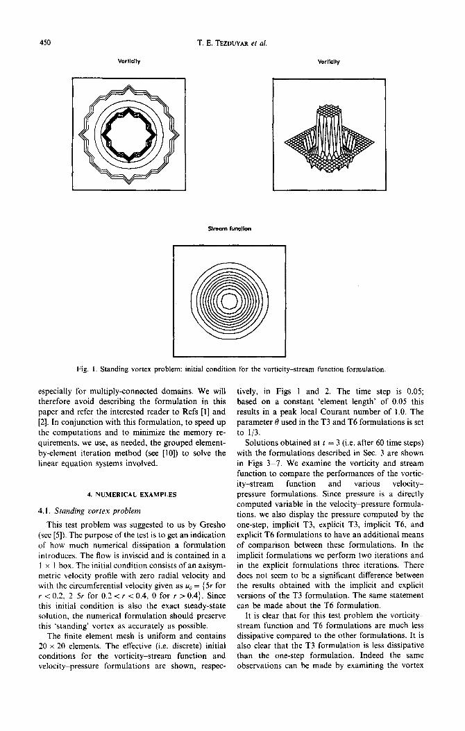
Fig. 1. Standing vortex problem: initial condition for the vorticity-stream function formulation.

especially for multiply-connected domains. We will therefore avoid describing the formulation in this paper and refer the interested reader to Refs [I] and [2]. In conjunction with this formulation, to speed up the computations and to minimize the memory re- quirements, we use, as needed, the grouped element- by-element iteration method (see [lo]) to solve the linear equation systems involved.

4. NUMERICAL EXAMPLES

4.1. Standing vortex problem

This test problem was suggested to us by Gresho (see [5]). The purpose of the test is to get an indication of how much numerical dissipation a formulation introduces. The flow is inviscid and is contained in a 1 x 1 box. The initial condition consists of an axisym- metric velocity profile with zero radial velocity and with the circumferential velocity given as u0 = { 5r for Y < 0.2, 2-5r for 0.2 < r < 0.4, 0 for r > 0.4). Since this initial condition is also the exact steady-state solution, the numerical formulation should preserve this ‘standing’ vortex as accurately as possible.

The finite element mesh is uniform and contains 20 x 20 elements. The effective (i.e. discrete) initial conditions for the vorticity-stream function and velocity-pressure formulations are shown, respec-

tively, in Figs 1 and 2. The time step is 0.05; based on a constant ‘element length’ of 0.05 this results in a peak local Courant number of 1.0. The parameter 0 used in the T3 and T6 formulations is set to l/3.

Solutions obtained at t = 3 (i.e. after 60 time steps) with the formulations described in Sec. 3 are shown in Figs 3-7. We examine the vorticity and stream function to compare the performances of the vorticity-stream function and various velocity- pressure formulations. Since pressure is a directly computed variable in the velocity-pressure formulations, we also display the pressure computed by the one-step, implicit T3, explicit T3, implicit T6, and explicit T6 formulations to have an additional means of comparison between these formulations. In the implicit formulations we perform two iterations and in the explicit formulations three iterations. There does not seem to be a significant difference between the results obtained with the implicit and explicit versions of the T3 formulation. The same statement can be made about the T6 formulation.

It is clear that for this test problem the vorticity- stream function and T6 formulations are much less dissipative compared to the other formulations. It is also clear that the T3 formulation is less dissipative than the one-step formulation. Indeed the same observations can be made by examining the vortex


velocity

-

I - llll -$ f

‘l\l’ 1.

Fig. 2. Standing vortex problem: initial condition for the velocity-pressure formulation.

452 T. E.TEZDUYAR et al.

lmpllclt TJ

lmpllcit T6

One-Step

Explkit TJ

Expllclt T6

@

0 0

Fig. 3. Solution of the standing vortex problem with various formulations: vorticity at t = 3.


lmpklt T3 tcprktt TS

Fig. 4. Solution of the standing vortex problem with various formulations: vorticity at 1 = 3.

454 T. E. TEZDUYAR et al.

knplldt T3 fiqWtT3

ImplIcit T6

Fig. 5. Solution of the standing vortex problem with various formulations: stream function at r = 3.


lmpliclt T3

ImplicIt T6 Explldt T6

Fig. 6. Solution of the standing vortex problem with various formulations: pressure at t = 3.


ImpkIt T3 Explklt 13

Imp(kit T6 Expllclt T6

Fig. 7. Solution of the standing vortex problem with various formulations: pressure at t = 3


Maximum CA,= 1.0

Maximum CA+= 0.5

0.5 1.0 I.5 2.0 2.5 i.0

Fig. 8. Solution of the standing vortex problem with various formulations: time history of the vortex kinetic energy.

kinetic energy, which is defined as vT.MLuMP.v/2. Figure 8 shows the time history of the vortex kinetic energy normalized by its initial value. For a peak local Courant number of 1.0 we see a substantial decay in the vortex kinetic energy obtained with the one-step and T3 formulations. At the end of the period of interest the vortex kinetic energy falls down to 22.7,48.5 and 48.6% for the one-step, implicit T3, and explicit T3 formulations, respectively. On the other hand we observe far less energy decay for the vorticity-stream function and T6 formulations. By the end of the test period the vorticity-stream function, implicit T6, and explicit T6 formulations retain, respectively, 99.7,97.3 and 97.8% of the initial vortex kinetic energy.

4.2. Flow past a circular cylinder

In this problem we compare the ‘steady-state’ and time-dependent solutions obtained with the vorticity- stream function, one-step, and explicit T6 formulations. We perform three iterations in the explicit T6 formulation. The dimensions of the computational domain, normalized by the cylinder diameter, are 30.5 and 16.0 in the flow and cross-flow directions, respectively. Figure 9 shows the various meshes employed in this problem. Mesh A consists of 1310 elements and 1365 nodes; around the cylinder there are 29 elements in the radial and 40 elements in the circumferential directions. Mesh B involves 5220 elements and 5329 nodes with 58 and 80 elements in the radial and circumferential directions. Mesh C contains 19,836 elements and 20,046 nodes with 116 and 156 elements in the radial and circumferential directions.

The upper and lower computational boundaries are taken as symmetry lines, as described in Sec. 2. The conditions imposed at the upstream and downstream boundaries for this type of problem are also described in Sec. 2. The Reynolds number is based on the uniform free stream velocity and the cylinder diameter. The time step used varies from one mesh to another. The parameter 8 used in the T6 formulation is set to l/3.

We first conducted a convergence study based on successive mesh refinement by examining the ‘steady- state’ solution at Reynolds number 100. Of course at this Reynolds number the ‘steady-state’ solution is not stable, and if the symmetry of the flow field is somehow perturbed then the solution becomes time- dependent and involves vortex shedding. However, in this case a ‘steady-state’ solution can be reached far before the machine truncation error perturbs the symmetry significantly. Nevertheless, we still would like to use the term ‘steady-state’ with caution.

Figure 10 shows the pressure coefficient, drag coefficient, wall vorticity, and separation angle corresponding to the ‘steady-state’ solution obtained with the vorticity-stream function formulation. Looking at these quantities we see that there is little difference between the solutions obtained with Meshes A and B; furthermore the difference between the solutions obtained with Meshes B and C is negligibly small. Figure 11 shows a similar trend for the one-step velocity-pressure formulation; in this case the differences are still small but not as small as they are in the case of the vorticity-stream function formulation. Based on this convergence study we conclude that it is reasonable to assume that the solutions obtained with Mesh B will be sufficiently accurate. Therefore for all computations that will be reported in the remainder of this paper we use Mesh B.

Next we investigated the variation of the ‘steady- state’ solution with Reynolds number by performing computations for Reynolds number 20, 40, 60, 80, and 100. Figure 12 shows the pressure and drag

458 T. E. TEZDWAR et d,

Mash A

Fig. 9. Flow past a circular cylinder: Mesh A (1310 elements and 1365 nodes); Mesh B (5220 elements and 5329 nodes); and Mesh C (19,836 elements and 20,046 nodes).


3 36.0 72.0 108.0 W.0

e

#O 36.0 72.0 IO&O u4.0 1 tJ

,O

Fig. 10. Flow past a circular cylinder at Reynolds number 100: ‘steady-state’ solution [pressure coefficient (C,), drag coefficient (C,), wall vorticity (o,), and separation angle (S,)] obtained with the vorticity- stream function formula-

tion using Meshes A, B, and C.

1 se.0 72.0 lOc..O i44.0 18

e

D 36.0 72.0 108.0 l44.0 1 e

I.0

1.0

Fig. 11. Flow past a circular cylinder at Reynolds number 100: ‘steady-state’ solution [pressure coefficient (C,), drag coefficient (C,,), wall vorticity (o,), and separation angle (@,)I obtained with the one-step formulation using Meshes

A, B, and C.


sll/_z_ 36.0 72.0 106.0 144.0 1

e

, 3b.O 7i.o Id6.0 i4i.o II

8

Fig. 12. Flow past a circular cylinder at various Reynolds numbers: ‘steady-state’ solution [pressure coefficient (c,,), drag coefficient (C,), wall vorticity (w,.), and separation angle (tl,)] obtained with the vorticity-stream function

formulation.

coefficients, wall vorticity, and separation angle obtained with the vorticity-stream function formulation. The same quantities obtained with the one-step and T6 formulations are shown in Figs 13 and 14, respectively. It is interesting to see that there is very little difference between the values obtained with the vorticity-stream function and T6 formulations. For example, for all five values of the Reynolds number the variation in the drag coefficient from one formulation to the other one is no more than 1.25%.

For Reynolds number 100 we also studied the time- dependent flow behavior by employing the vorticity- stream function, one-step, and T6 formulations. For each formulation we started with the ‘steady-state’

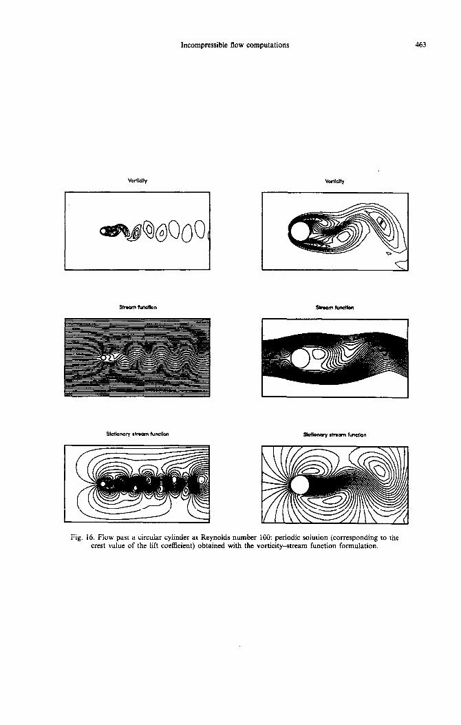
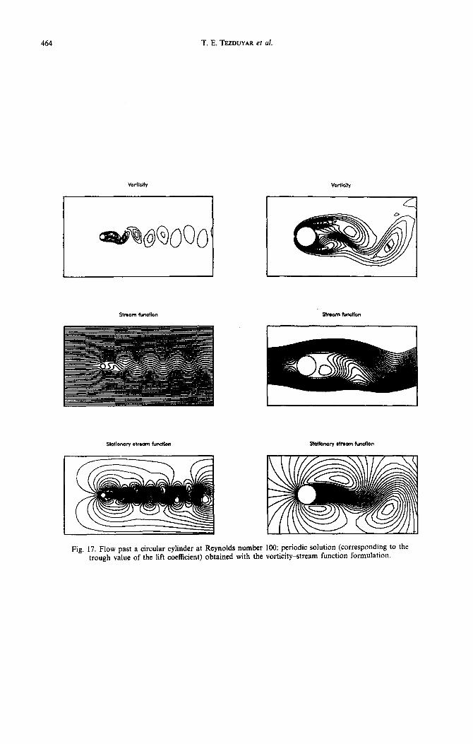
solution obtained with that formulation, and initiated the time-dependent flow by introducing a short-term perturbation to the symmetric flow field. Figure 15 shows the ‘steady-state’ solution obtained with the vorticity-stream function formulation. For the same formulation, Figs 16 and 17 show the periodic flow patterns corresponding to the crest and trough values of the lift coefficient. The ‘steady-state’ and periodic flow patterns are shown in Figs 18-20 for the one-step formulation, and in Figs 21-23 for the T6 formulation. We notice some differences in the wake patterns obtained by the three formulations. These differences are more significant between the one-step formulation and the vorticity-stream function and T6 formulations; we believe that this is because the one- step formulation is numerically more dissipative than the others. The less significant differences between the vorticity-stream function and T6 formulations might be due to the differences in the downstream boundary conditions. Finally, Figs 24 and 25 show the time history of the drag and lift coefficients obtained with the three formulations. By examining the time history of the lift coefficient, we estimate the Strouhal number to be 0.171, 0.154, and 0.173 for the vorticity- stream function, one-step, and T6 formulations, respectively.

5. CONCLUSIONS

We have presented our finite element procedures and computations based on the velocity-pressure and vorticity-stream function formulations of incompressible flows.

Two new multi-step velocity-pressure formulations have been proposed. In the T3 formulation the SUPG supplement is used only for the step in which the convective terms are treated implicitly. In the T6 formulation this supplement is further restricted to the sub-step involving only the convective terms. We compared these multi-step formulations with the vorticity-stream function and one-step velocity- pressure formulations.

Two numerical examples were picked: the standing vortex problem and flow past a circular cylinder. The purpose of the standing vortex problem was to compare the numerical dissipation characteristics of the various formulations considered. For this problem the vorticity-stream function and T6 formulations were much less dissipative than the one-step and T3 formulations. Furthermore, the T3 formulation was significantly less dissipative than the one-step formulation.

For flow past a circular cylinder we performed benchmark quality computations using the vorticity- stream function, one-step, and T6 formulations. In this problem, first we established the sufficiency of our mesh refinement by conducting a convergence study based on the successive mesh refinement. Next we computed the ‘steady-state’ solution for Reynolds number 20, 40, 60, 80, and 100. When we examined


/

0.1 0 36.0 7i.o loil.0 l4i.o 1

a

0 36.0 72.0 108.0 u4.0

e

0

.O

Fig. 13. Flow past a circular cylinder at various Reynolds numbers: ‘steady-state’ solution [pressure coefficient (C,), drag coefficient (C,), wall vorticity (w,), and separation

angle (S,)] obtained with the one-step formulation.

LEGEND 0 = Re= 20. C&.210 -----I 0 = Re.= 40, C,=1.629 A = Re= 60, Cd=1.390 + = Re= 80, C,=1.259 x = Re=lOO. C,=l.l79

1 38.0 72.0 108.0 lii.0 1 8

LEGEND 0 = Re= 20, @,=136.2 0 = f?e= 40, 8,=126.1* A = Re= 60, f3,=120.7’ + = Re= 80. 9,=116.8’ x = Re=lOO, 9,=1l4.2’

0 38.0 72.0 108.0 l44.0 1 e

1.0

3.0

Fig. 14. Flow past a circular cylinder at various Reynolds numbers: ‘steady-state’ solution [pressure coefficient (C,), drag coefficient (C,), wall vorticity (w,), and separation

angle (OS)] obtained with the T6 formulation.


Vorticity

Y

Strewn function stmm functton

I I

Fig. 15. Flow past a circular cylinder at Reynolds number 100: ‘steady-state’ solution obtained with the vorticity-stream function formulation.


Fig. 16. Flow past a circular cylinder at Reynolds number 100: periodic solution (corresponding to the crest value of the lift coefficient) obtained with the vorticity-stream function formulation.

T. E. TEZDUYAR el ai.

Shorn funclbn SfrMln funclbil

Sldbneq ha functbn

Fig. 17. Flow past a circular cylinder at Reynolds number 100: periodic solution (corresponding to the trough value of the lift coefficient) obtained with the vorticity-stream function formulation.


Votiklty

Sidkmy ctnom functkm Sbtbmry dream fundbn

Fig. 18. Flow past a circular cylinder at Reynolds number 100: ‘steady-state’ solution obtained with the one-step formulation.


Vwticity

Fig. 19. Flow past a circular cylinder at Reynolds number 100: periodic solution (corresponding to the crest value of the lift coefficient) obtained with the one-step formulation.

Incompressible Bow computations 46-l

Fig. 20. Flow past a circular cylinder at Reynolds number 100: periodic solution (corresponding to the trough value of the lift coefficient) obtained with the one-step formulation.


Vartiiiy

Shcm functleo

Fig. 2 I Flow past a circular cylinder at Reynolds number 100: ‘steady-state’ solution obtained with the T6 formulation.


Vortkity

statt0na-y hurl function

I i

Fig. 22. Flow past a circular cylinder at Reynolds number 100: periodic solution (corresponding to the crest value of the lift coefficient) obtained with the T6 formulation.

Ls 35&.-M

470 T. E. TEZDUYAR et nf.

Vorlicity

I

statbnary bfmam fundion

Fig. 23. Flow past a circular cylinder at Reynolds number 100: periodic solution (corresponding to the trough value of the lift coefficient) obtained with the T6 formulation.

Vo

rtic

ity-

stre

am

fun

ctio

n

form

ula

tio

n

1.25

On

e-st

ep

form

ula

tio

n

1.25

T6

form

ula

tio

n

1.45

1.25

1.15

0

200

400

600

600

1000

12

00

9400

Fig.

24

. Fl

ow

past

a

circ

ular

cy

linde

r at

R

eyno

lds

num

ber

100:

tim

e hi

stor

y of

th

e dr

ag

coef

fici

ent

(C,)

ob

tain

ed

resp

ectiv

ely

with

th

e vo

rtic

ity-s

trea

m

func

tion,

on

e-st

ep,

and

T6

form

ulat

ions

.

Vo

rtic

ity-

stre

om

fu

nct

ion

fo

rmu

lati

on

0.25

-0.2

5

-0.5

0 0

200

400

600

600

1000

12

00

1400

On

e-st

ep

form

ula

tio

n

0.25

-0.2

5

-0.5

0 0

200

400

600

600

4000

12

00

1400

T6

form

ula

tio

n

0.25

o-1

’ “‘

I’ II

II I

I II

I 1

I I

I I

I

i !

” I

-0.2

5-

\/ I

1 I

I I

VV

ViH

lV

-0.5

07

!

0 20

0 40

0 60

0 60

0 10

00

‘120

0 14

00

Fig.

25

. Fl

ow

past

a

circ

ular

cy

linde

r at

R

eyno

lds

num

ber

1001

Str

ouha

l nu

mbe

r (S

t)

and

the

time

hist

ory

of

the

lift

coef

fici

ent

obta

ined

, re

spec

tivel

y,

with

th

e vo

rtic

ity-s

trea

m

func

tion,

on

e-st

ep,

and

T6

form

ulat

ions

.

_,, ,-

_,

_

. ,,,

,, I-

I..“,

. “,

_

._. -

- .._

. . ._

-

_ . .

_ .,~

,”

.


the pressure and drag coefficients, wall vorticity, and separation angle, we observed very littie difference between the values obtained with these different formulations. We noticed more significant differences in the wake of the cylinder. We also studied the time-

dependent flow at Reynolds number 100. The time- dependent behavior involves vortex shedding and is,

in the long run, periodic in time. In this case the differences in the solutions obtained with different formulations were more significant. By examining the frequency and amplitude of the lift and drag varia- tions we could see that the vorticity-stream function and T6 formulations were less dissipative than the

one-step fo~ulation. Once again we note that the dissipation characteristics of a formulation are very important if we are interested in the wake and/or time-dependent behavior of this type of problems,

Ackn~~~~edgen~ents -This research was sponsored by the NASA-Johnson Space Center under contract NAS-9-17892 and by the NSF under grant MSM-8796352.

REFERENCES

T. E. Tezduyar, J. Liou and R. Glowinski, Petrov- Galerkin methods on multiply connected domains for the vorticity-stream formulation of the incompressible Navier-Stokes equations. Int. J. Numer. Meth. Fluids 8, 1269-1290 (1988). T. E. Tezduyar, Finite element formulation for the vorticity-stream function form of the incompressible

3.

4.

5.

6.

I.

8.

9.

10.

Euler equations on multiply-connoted domains. ~~rn~~l. Meth. appl. Mech. Engng 73, 331-339 (1989). A. N. Brooks and T. J. R. Hughes, Steamline-upwind/ Petrov-Galerkin formulations for convection dominated flows with particular emphasis on incompressible Navier-Stokes equation. Comput. Meth. appl. Mech. Engng 32, 199-259 (1982). M. 0. Bristeau, R. Glowinski and J. Periaux, Nu- merical methods for the Navier-Stokes equations; applications to the simulation of compressible and incompressible viscous flows. Comput. Phys. Repor 6, 73-187 (1987). P. M. Gresho and S. T. Chan, Semi-consistent mass matrix techniques for solving the incompressible Navier-Stokes equations. Lawrence Livermore National Laboratory Preprint, LJCRL-99503. M. Braza. P. Chassaina and H. H. Minh. Numerical study and’physical anal&is of the pressure and velocity fields in the near wake of a circular cylinder. J. Fluid Mech. 165, 79-130 (1986). T. E. Tezduyar and D. K. Ganjoo, Petrov-Galerkin formulations with weighting functions dependent upon spatial and temporal discretization: application to tran- sient convection diffusion problems. ~~rnput. Met/r. appl. Me& Engng 59, 49.--71 (1986). R. Glowinski, Numericuf Methods _for Nonlinear Vuriationul Problems. Springer, New York (1984). T. E. Tezduyar. J. Liou, D. K. Ganjoo and R. Glowinski, Solution techniques for incompressible flow problems. In Finite Element An&sis in Fluids (Edited by T. J. Chung and G. R. Karr), pp. 836-844. UAH Press, HuntsviIle, AL (1989). T. E. Tezduyar and J. Liou, Grouped element- by-element iteration schemes for incompressible Bow computations. Cumput. Ph~‘x Commun. 53, 441.-453 (1989).

incompressible flow computations based on … · incompressible flow computations based on the...

Documents