INCORPORATING DOMAIN KNOWLEDGE OF GENERALIZED TONIC-CLONIC

SEIZURES INTO SEIZURE ONSET DETECTOR ON AN APPLE WATCH USING

NEURAL NETWORK

by

Michael Chan

A thesis submitted to Johns Hopkins University in conformity with the requirements for the

degree of Master of Science in Engineering

Baltimore, Maryland

May, 2019

© Michael Chan 2019

All rights reserved

ii

ABSTRACT

Generalized tonic-clonic seizures (GTCS) is the most severe type of seizure that could lead to sudden

unexpected death in epilepsy (SUDEP). To solve this problem, we’ve previously built a seizure onset

detector on Apple Watch to serve as an alerting system for timely intervention. The detector was able to

achieve a sensitivity of 95%, 2 false positives per day, and a 60 seconds latency in detection. To further

optimize the development process of the detector and its performance, we constructed a machine learning

model pipeline, explored different feature sets, and incorporated domain knowledge to neural network

models. We’ve determined that spectral features outperformed handcrafted features. We’ve also designed

neural networks based on the domain knowledge by modeling time and/or frequency dynamics. In

particular, a F-LSTM/T-LSTM NN was able to reach a targeted performance of 100% sensitivity, 0.41

false positives per day, and a mean of 6.87 seconds latency in detection. In the future, we will package

our software, explore the use of other modules on Apple Watch to maximize its use, and design a

personalized detector when we have a larger dataset.

Thesis Committee Chair: Dr. Nathan E. Crone

Thesis Project Adviser and Thesis Committee Member: Dr. Shinji Watanabe

Thesis Committee Member: Dr. Sridevi V. Sarma

iii

PREFACE

I would first like to thank my thesis advisor Dr. Nathan Crone of the Neurology department at Johns

Hopkins Medicine for his mentorship and support. Dr. Crone has always been eager to discuss research

related problems with me. I am also grateful for the opportunity to explore potential research direction for

the EpiWatch project.

I would like to also my thesis committee members: Dr. Shinji Watanabe and Dr. Sridevi V. Sarma. I have

learned a lot of technical skills and domain know-how from Dr. Watanabe. I’ve enjoyed every

conversation we had because they helped incubate new ideas for this thesis. Dr. Sarma has been helpful in

providing me necessary guidance to complete this thesis.

Finally, I’d like thank my colleagues in Dr. Crone’s lab, Maxwell Collard, Samyak Shah, Daniel Candrea,

Tessy Thomas, Qinwan Rabbani, Anna Korzeniewska, Christopher Coogan, Alexander Weiss, Yujing

Wang, and Griffin Milsap for the stimulating conversations we had during lunchtime.

iv

DEDICATION

I would like to dedicate this thesis to my family and friends. Thank you for having confidence in me and

encouraging me to pursue my passion. I also dedicate this to all my teachers and professors who have

been the reason for my passion and love for science.

Finally, I would like to express my profound gratitude to my parents and friends. I’ve adapted dedication,

motivation, curiosity, critical thinking, etc. from them, which made me the mature and independent

researcher I am today. For the amazing people I will meet, for the cool stuff I will build, for the dreams

that will come true, and for the moments that I look back, I never stop.

v

TABLE OF CONTENTS

Chapter 1: Introduction .………………………………………………………………...........................1

1.1. Epilepsy, seizure, SUDEP .…………………………………….….…...…………………...…...........1

1.2. Intro to seizure onset detector .………………………………...….….…...……………………….....2

1.3. Current achievements .……….……………………………….….…...………………………........... 3

1.4. Thesis Overview .………………………..…………………….….…...………………………...........5

Chapter 2: EpiWatch Development Environment 6

2.1. Previous work .…………………………..…………………….….…...………………………...........6

2.2. Data preprocessing pipeline .…………….…………………….….…...………………………...........8

2.2.1. Stage 1 - data ingestion .………………………..………………………...….…...…………………9

2.2.2. Stage 2 - data preparation .………………………..…………………….….….……………...........10

2.2.3. Stage 3 - feature extraction.………………………..…………………….…....……………........... 11

2.2.4. Stage 4 - model training and optimization .………………………....………………………...........11

2.2.5. Stage 5 - model conversion .………………………..…………….....………………………...........12

2.3. Summary .………………………..…………………………....….…...………………………...........12

Chapter 3: Feature exploration .………………………..……….….…...………………………...........15

3.1. Introduction to different feature extraction methods .………….…......………………………...........15

3.2. Handcrafted features .………………………..…………………….….…...……….…………...........16

3.3. Spectral features .………………………..…………………….…...….…...…………………............20

vi

3.4. LSTM neural network architecture .………………………..…………..……………………...........24

3.5. Performance: sensitivity, specificity, latency, and computation time .………………………...........26

3.6. Summary .………………………..…………………….….….........................………………...........29

Chapter 4: Incorporate domain knowledge into neural network architecture .…...……………….30

4.1. Introduction .………………………..…………………….….…...……………….…………...........30

4.2. How to Domain knowledge: chirp in motion signal in GTC seizure .…………….…………...........30

4.3. Advanced seizure onset detector using neural network: LSTM that capture time and frequency

dynamics .……………………….…………………………………….……..........………………...........32

4.4. Training recipe and K-fold cross validation .……… ………..….…...………………………...........34

4.5. Performance: sensitivity, specificity, latency, computation cost .……....……………………...........35

4.6. Summary .………………………..……..…………………….….…...………………………...........37

Chapter 5: Conclusion and future directions .……… ……………………...…………………...........38

5.1. Future direction .………………………..…………………….….…...………………………...........38

5.1.1. Build Python pip packages and unit tests for maintainability .…….….……………………...........38

5.1.2. The use of microphone: detector targeted for ictal cry . ……….….……..…………...……...........38

5.1.3. The use of speaker: vocal instruction for timely intervention ………..……………………...........39

5.1.4. Evaluation of the duration of postictal generalized EEG suppression for better SUDEP risk

assessment.……………………………….....…………………….….…...………………………........... 39

5.1.5. Personalized detector .…………………………………...…….…...………………………...........40

5.2. Conclusion .………………………..…………………….……....…...………………………...........40

vii

LIST OF TABLES

Chapter 1:

1.1. Performance metrics for seizure onset detector .………………………..…………… ………...........2

Chapter 2:

2.1. Description of the notebook pipeline that trains and optimizes an iForest detector .………………...7

Chapter 3:

3.1. Definition of TP, FP, FN, and TN .………………………..…………………………………………26

3.2. Classification performances of handcrafted features and spectral features are compared …………..27

Chapter 4:

4.1. Observations on the characteristics of the chirp .………………………..…………………………...31

4.2. Feature extraction constraints based on prior knowledge about chirp .……………………………....31

4.3 Performance for different LSTM approaches .………………………..……………………………....36

viii

LIST OF FIGURES

Chapter 2:

2.1. The proposed machine learning pipeline .………………………..…………………………………..9

2.2. Data preprocessing visualization .………………………..………………………………………….10

2.3. Data is segmented using a user defined epoch size and overlap .………………………..………….11

2.4. Flow chart of CoreML model conversion .………………………..………………………………...12

2.5 Cyclical machine learning pipeline .………………………..………………………………………..13

2.6. A sample snippet of pipeline shell script with the 5 stages scheme .………………………..………14

Chapter 3:

3.1. Zero-crossing points .………………………..………………………………………………………17

3.2. Raw data and handcrafted features .………………….. ….…………………………………………19

3.3. Spectral features distribution .………………..………………………...……………………………20

3.4. Sample seizure and non-seizure data in time and frequency domain .…………………...…………21

3.5. Distributions of the spectral features before standardization of seizure and non-seizure data…….. 22

3.6. Spectrogram contracted from spectral feature vectors (1~20Hz) .…………………………... …… 23

3.7. Frequency features have a lot of information .………………………..…………………………… 24

3.8. The LSTM NN architectures for both handcrafted features and spectral features …………………25

3.9. Latency definition .………………………..………………………………………………………...26

3.10. The ROC curves and latency curves for both handcrafted and spectral feature set are compared ..28

3.11. Outputs of both detectors on all 15 seizure data stacked together.…………………………..……..28

ix

Chapter 4:

4.1. TF-LSTM NN architecture .………………………..………………………………………………..33

4.2. F-LSTM/T-LSTM NN architecture .………………………..……………………………………….34

4.3. The ROC curves and latency curves for both handcrafted and spectral feature set ………………...37

4.4. LSTM NN output for all four LSTM models ……………………………………………………….37

1

Chapter 1: Introduction

1.1. Epilepsy, SUDEP, GTC seizure

Of the 3 million Americans with active epilepsy, approximately 1 million continue to have uncontrolled

seizures even with ongoing medical therapy (Tian, 2018). While epilepsies, the seizure types experienced

by patients, and the impacts on quality of life associated with individuals’ seizures are incredibly diverse,

generalized tonic-clonic convulsions are a particular focus of study. These seizures—especially those that

are prolonged or violent—are at-risk for major complications including sudden death in epilepsy

(SUDEP), which occurs in approximately 1 in 100 patients with uncontrolled GTCS per year (Ficker et

al., 1998). While uncontrolled GTCS are particularly correlated with SUDEP (Ficker & Ficker, 2000),

recent evidence indicates that timely intervention during the course of, and immediately following, a

convulsion can substantially reduce the risk of SUDEP and other complications (Ryvlin et al., 2013).

Therefore, a great deal of recent interest has been focused on developing means of detecting GTCS in real

time, and of alerting caregivers or emergency services to these detected events (Tzallas et al., 2012).

There are a series of stages in a GTCS including aura, tonic, clonic, and postictal stages. In aura stage,

patients could experience hallucination, confusion, numbness, and distorted emotions. In tonic stage,

patients could experience epileptic cry (ictal cry), stiff body, incontinence, back arched. In clonic stage,

there will be a distinctive rhythmic motion, frothy saliva, and blinking eyes. In postictal stage, patients

will have weak limbs, exhaustion, sleepy. SUDEP normally occurs after the clonic stage, in which

patients are in or after the postictal stage. There was often breathing difficulty before death. A study in

1996 has shown that 59% of patients developed apnea and 35% developed oxygen saturation in the range

of 55% to 83% during seizures, suggesting that seizures can lead to life-threatening event such as cardiac

and respiratory dysfunction. (Nashef et al., 1996).

2

We believe that a warning device that is triggered by the characteristic movement occurring at the tonic-

clonic stage (especially clonic stage) is most helpful to prevent SUDEP, so intervention can be applied

timely by care givers. A detector needs to reach near perfect sensitivity to fully prevent SUDEP. While

100% sensitivity is relatively easy to attain, it usually comes at the cost of higher false positive rate (FPR)

and unacceptably long latency. The detector needs to have low FPR to be useful to the patients. Frequent

false alarms can greatly reduce device adherence and therefore lose its purpose. We envisioned a detector

for nocturnal monitoring at home so family members can reach the patients in time at nighttime. We also

expected usage under ambulatory setting, where patients are active and sometimes outdoor. Patients can

have a peace of mind when being alone. In both cases, latency of the detector needs to be less than 60

seconds.

Sensitivity FPR Latency

Minimum requirement > 95% < 0.2 per day < 60 seconds

Table 1.1. Performance metrics for seizure onset detector.

1.2. Intro to seizure onset detector

To reduce SUDEP, many teams have invested in designing the hardware component of seizure onset

detector for research and commercialization. Different sensors have been investigated and each shows

their strengths and weaknesses. Electroencephalogram (EEG), usually paired with video recording

(vEEG), is the most accurate method for seizure labeling since it targets the source of seizure: brain. It is

often used as a gold standard device for epileptologists to label seizure stages. However, it does limit

mobility and portable EEG is uncomfortable to wear (Bell, Walczak, Shin, & Radtke, 1997). Patients

usually feel uneasy to wear them in public. On the other hand, in-bed sensor strips are the most

comfortable alternatives with the lowest sense of presence. It can extract heart rate and respiratory rate

with its piezoelectric sensor strips. They do not limit patients’ mobility as they are not placed on the

3

patients but on top of mattress pad. Nevertheless, its inability to realize ambulatory monitoring prevents it

from becoming a universal solution for seizure onset detection. There are other electrophysiological

signals that can provide important insights such as disruptions in nervous system. Since 70% of the

patients have cardiovascular dysfunction during seizures, electrocardiogram (ECG) can be used to extract

heart rate and advanced cardiovascular information (Vandecasteele et al., 2017). Electromyography

(EMG) has good performance since limb movements caused by GTCS are distinctive from other

movement while consistent among itself (Hamer, 2003). Nevertheless, common ECG and EMG

electrodes, Ag/Cl electrodes, can cause skin irritation, so they are not ideal solution for long-term

monitoring (longer than 12 hours). Ideal sensor choice should be portable, noninvasive, and comfortable.

Wrist-worn devices have emerged in particular force, owing to their unobtrusiveness, ease of use, and the

ability to house several noninvasive sensors. While the majority of these devices utilize accelerometry as

their primary modality, several other classes of sensors have also been successful at informing seizure

detection, including heart rate data derived from photoplethysmography (PPG) data (Vandecasteele et al.,

2017), as well as sympathetic response derived from electrodermal activity (EDA) (Poh et al., 2012) and

motion features extracted from accelerometer (ACC) data (Beniczky, Polster, Kjaer, & Hjalgrim, 2013).

1.3. Current achievements

Here we introduce and test the performance of a seizure detection and alerting system, EpiWatch,

developed on a commercially available consumer wearable device, Apple Watch. Motivated by recent

evidence that suggests that the biosensor readings measured by Apple Watch are highly accurate (El-

Amrawy & Nounou, 2015), we developed a detection algorithm that fuses the movement data provided

by accelerometer with heart rate measurements computed from the built-in PPG sensor in Apple Watch.

As GTCS are relatively rare events, we utilized a novelty detection strategy called an Isolation Forest

(iForest), well-tailored to imbalanced classification problems. We built a candidate detector using a

4

dataset collected from a combination of inpatients in an epilepsy monitoring unit (EMU) and ambulatory

controls without epilepsy. In a prospective “evaluation” dataset, we measured sufficient performance to

potentially provide real-world utility as a seizure detector. Currently, we have 9 seizures labeled by

vEEG, about 2 hours of recording. Control data (non-seizure data) last about 4000 hours.

Seizure detection is done by evaluating continuous “epoch,” a 1 second worth of data. Handcrafted

features extracted from data in each epoch will be used as the input of the detector to better represent the

data. The detector, iForest, will act as an anomaly detector that determines whether an epoch represents a

normal or abnormal behavior. It is trained by feeding nearly 4000 hours of non-epileptic data. Intuitively,

any anomaly data (such as epileptic convulsion) can trigger iForest and lead to the firing of the detector.

Since the epoch is 1 second long, the output of iForest will have a detection rate of 1 detection / second.

Although this method yields high sensitivity in our preliminary testing, it can also trigger many false

positives for usual activities not related to epilepsy, such as tooth brushing or exercise. Therefore, we

introduce a subsequent mechanism to reduce the false positives: evidence accumulation. Evidence

accumulation acts as a smoothing filter. Only when the output of the evidence accumulation stage reaches

beyond threshold, the detection system will respond and follow with intervention logics (confirm user’s

conscience and alert caregivers).

Despite the success made by EpiWatch has been promising, we believe that we haven’t maximized the

use of the data collected and the superior resources Apple Watch has offered for developers. Since the

development of EpiWatch seizure detector has been in the feasibility stage, it was important to assure

whether we can build a functioning seizure detector on Apple Watch. The underlying difficulties include

sensor data intact retrieval, battery consumption, CPU usage limitation, etc. The strategy taken was to

build a minimum viable product (MVP). Through the process, we learned that data retrieval can

occasionally fail in earlier versions (Watch Series 2 and 3) while haven’t failed in the latest version

(Watch Series 4). Battery consumption hasn’t been a problem since Series 3, largely due to the more

5

efficient CPU (Apple S3 Silicon in Package) Apple developed. We also learned that we have CPU usage

to spare (we only used 8% for the current build), which opens opportunities to research in advanced

algorithms such as neural network. Note that the choices of feature extraction and detection methods are

constrained by computation resources and the size of our dataset. Although this method has been

performing well in sensitivity and slightly improve the specificity, the specificity is still not acceptable

(2/day). Evidence accumulation can certainly improve specificity, it also hinders latency significantly (it

takes at least 10 “anomaly” epochs, or 10 seconds for the detector to trigger). It is merely a crude way to

capture time dynamics: It relies on the fact that GTCS usually last more than 10 seconds. It does not learn

the characteristics of GTCS as time progresses. In addition, iForest can only output binary results, which

makes its prediction imprecise. Now that our current build has answered the feasibility question, we

should ask the next question to ourselves: can we build a high-performing seizure detector on Apple

Watch?

1.4. Thesis Overview

To move from MVP to Minimum Marketable Product (MMP), it is important to first construct a machine

learning model pipeline for efficient collaboration. The hardware and the supported API have also

improved significantly (from Watch Series 1 to Watch Series 4), we are ready to make some changes. It is

evident from the above that the current detector should be replaced with a more advanced one. To build a

more advanced algorithm, the model needs to learn the structure in the data (e.g. dynamics in frequency

and time). It should abandon evidence accumulation as there should exist better methods to reduce FPR.

As a result, there is a need to critically evaluate the feasibility and quality of different feature sets, assess

the performance mathematical models corresponding to each feature sets, and select the best model

accordingly.

6

This thesis is organized in the following order: In Chapter 2, a well-structured pipeline to perform

machine learning model production will be discussed. To advance the algorithm, our MMP will focus on

reaching the high-performing metrics found in literature (sensitivity of 90%, FPR of <0.5 per day, and

latency < 60 seconds) by optimizing feature extraction and classification separately. In Chapter 3, two

feature extraction methods, handcrafted features and spectral features, are tested and compared. In

Chapter 4, neural network models that utilize the spectral feature set and incorporate domain knowledge

in GTCS are discussed. Four variants of the long short-term memory (LSTM) neural networks come from

literature, one of the variants is proposed by the author. The four models will be tested and compared

based on their performance and computation cost. Finally, future research direction will be proposed and

explained in detail in Chapter 5.

7

Chapter 2: EpiWatch Development Environment

2.1. Previous work

EpiWatch algorithm development was started by a student researcher who developed a software pipeline

that produces a GTCS onset detector. Specifically, this pipeline performs preprocessing, feature

extraction, model training and optimization, and model serialization for mobile device deployment on

Jupyter notebooks, an open source web application that can be used to create documents that contain

code, visualizations, and text. A table that describes and evaluates this pipeline is provided below:

Purpose Export what What I learned

notebook 1: setup data retrieval from

backend, filtering,

plotting

filter parameters plots are well labeled

and organized, can

reuse the code

notebook 2: seizures inspect seizures data export seizure

descriptors back into

local database

labels (fineStart and

fineEnd) are logged by

our epileptologists

notebook 3: pull show statistics of the

data, show number of

records by user and

total data duration

(~4000 hrs)

save intermediate data

at local machine pulling data is time

intensive, this pipeline

has an efficient way to

mitigate this

notebook 4: preprocess chunk, uniformize, and

filter data export preprocessed

seizure data export seizure and non-

seizure data separately

notebook 5: extract extract all features export feature vectors uses parallelization a lot

(faster)

notebook 6: select select features (9 of

them) export selected feature

names select features based on

ease of implementation

and interpretability

notebook 7: train z score plot, train and

evaluate an iForest

detector (use CV to

further optimize), ROC

plot

export detector

parameters as JSON detector parameters are

optimized in this

notebook, many

reusable codes

Table 2.1. Description of the notebook pipeline that trains and optimizes an iForest detector.

These notebooks are great in that the code is clean and well-documented. One can easily learn this

pipeline by executing all notebooks. The plots generated are well labeled and easy to interpret, while

8

providing insights to seizure data for new developers. Nevertheless, there are a few shortcomings. First of

all, the data are exported to folder that doesn’t have traceable name. For example, data exported in

notebook 3 are called “intermediates,” which is not self-explanatory. Secondly, the notebooks can’t be

run in background nor in terminal in a single software command, which makes certain time-consuming

tasks infeasible. This is important because new seizure data is generated constantly and our dataset is still

expanding. We’d like to have a system that automatically retrain the detector frequently. The notebooks

are also hard to be maintained by nature because one needs to open the notebook and run all cells to

debug. Further, current version control tool for changes tracking such as git does not provide support for

Jupyter notebooks, which hinders collaboration. The current pipeline is sufficient for research purposes,

but it is necessary to reform it to production level.

2.2. Data preprocessing pipeline

To reform the pipeline, we tried to first learn how other fields did it. For researchers in speech

recognition, Kaldi is a highly adopted toolkit. The main purpose of this toolkit is to encourage open

source collaboration by organizing speech recognition processing steps in “stages” so researchers don’t

have to reinvent the wheel. Stage is an important feature of Kaldi because it defines clear boundary of

each processing step. For example, a researcher might be interested in how a new feature extraction

method, a processing step of speech recognition, can help a speech recognition task. This researcher can

easily replace Kaldi’s feature extraction method with his/hers own while reuse the rest of the stages in

Kaldi to produce a speech recognition system with minimal development time. Similarly, our pipeline

also adapts the stage scheme. In the script, developers can replace any of the stage with his/her own recipe

as long as the input and output data have format equivalent to that in the same stage.

In a pipeline we designed, there are 5 stages, each can be run using a single shell script in the operating

system background and unit tests were provided for maintainability. In this pipeline, each stage can have

9

its own variants. For example, stage 3 (feature extraction) can have the following variants: handcrafted

features, spectral features, convolutional autoencoder features, etc.

Figure 2.1. The proposed machine learning pipeline.

2.2.1. Stage 1 - data ingestion

In this stage, raw data is first extracted from backend (MongoDB and AWS) using metadata in a JSON

file. Raw data has problems such as uneven sampling of both accelerometer and heart rate data, data gaps,

and data overlap. These problems can be mitigated by interpolation and data slicing. The processed data is

then filtered with a bandpass filter (0.2~20 Hz) to remove DC drifting and high frequency noise.

10

Figure 2.2. Data preprocessing visualization. The first plot shows the raw data that was retrieved from the

backend with no preprocessing. The second plot is interpolated and filtered. Purple color is used to

specify the segment of a seizure occurrence.

2.2.2. Stage 2 - data preparation

In this stage, data is segmented into epochs of equal length with user defined overlaps. Each epoch will be

assigned a seizure number (i_seizure), specifying the unique recording it belongs to. This is essential to

enable k-fold cross validation testing to ensure generalizability. The epochs will be stored in a matrix with

a dimension of (Nepochs, epoch length, # of channels), where the number of channels in this matrix is 4,

including accelerometer x-axis, y-axis, z-axis and heart rate channel. In addition, a vector of classes label

(binary, sz or non-sz) for each epoch is stored, with a dimension of (Nepochs, 1), and a vector of i_seizure

label (discrete integers) for each epoch is also stored, with a dimension of (Nepochs, 1).

11

Figure 2.3. Data is segmented using a user defined epoch size and overlap.

2.2.3. Stage 3 - feature extraction

This stage performs the feature extraction. Three feature extraction methods implemented include

handcrafted features, convolutional autoencoder features, and spectral features. The specifics of these

feature sets will not be discussed here. Since we plan to employ machine learning algorithms that capture

time dynamics, we will expand the extracted features to sequence of features. As a result, we have three

more feature set: handcrafted features sequence, convolutional autoencoder features sequence, and

spectral features sequence. A process called train-validation split is performed here for K-fold cross

validation. This stage is also similar to a dimensionality reduction step, so the data exported is very

similar to that in stage 2 (with lower data dimension).

2.2.4. Stage 4 - model training and optimization

In stage 4, different models are designed, trained, and tested. These models include iForest, SVM, and

LSTM models for handcrafted features, an LSTM model for convolutional autoencoder features, and

different variants of LSTM models for spectral features. It is important to train a model without

overfitting or underfitting, but such conditions cannot be predicted prior to training. Therefore, model

performance metrics (sensitivity, false positive rate, and latency) are recorded during training to estimate

12

bias and variance of the model trained. Our goal is to train a model that yields a low bias and a low

variance.

2.2.5. Stage 5 - model conversion

This stage is the last stage of the pipeline. It is relatively simple since the CoreML API provides most of

the software abstractions necessary for machine learning model deployment. CoreML is Apple’s machine

learning framework that is optimized for on-device performance for both iOS and Watch OS systems,

which minimizes memory footprint and lower power consumption. It allows app to provide machine

learning prediction (whether a recording is a seizure or not) even when there is no network connection. In

this stage, CoreML models are generated using the models trained in Python framework, and CoreML

models can be directly imported into the EpiWatch app.

Figure 2.4. Flow chart of CoreML model conversion

2.3. Summary

We’ve identified the problems of existing pipeline and proposed a reformed pipeline. The new pipeline

allows us to expand collections of feature set and models quickly and efficiently. Exploration of feature

extraction methods, model implementation, validation, and fine-tuning are all made automatic and

therefore, less time-consuming. For these reasons, this pipeline strengthens many aspects of EpiWatch

including work described in the following section. Future direction for this pipeline is to make it data

flow cyclical rather than one-way (see Figure 2.5) This change will iterate every step to continuously

improve the accuracy and generalizability of the model. A sample shell script of the pipeline is shown in

Figure 2.6.

13

Figure 2.5 Cyclical machine learning pipeline.

14

Figure 2.6. A sample snippet of pipeline shell script with the 5 stages scheme.

15

Chapter 3: Feature exploration

3.1. Introduction to different feature extraction methods

To build a more advanced algorithm, it is important to first re-examine our feature choice. Both

accelerometer and heart rate signals contain useful information. Tachycardia is a common symptom of

many types of seizures, including GTC seizures (Zijlmans, Flanagan, & Gotman, 2002). Information

hidden in heart rate data is relatively straightforward. The features used in our current detector are heart

rate amplitude and its derivative. Although advanced heart rate features such as heart rate variability

(HRV) can potentially contribute to discriminating power of the detector, the sampling rate of our heart

rate sensor is insufficient to support such analysis. As a result, we will only explore feature extraction

methods for accelerometer data.

On the other hand, accelerometer data contains more information. Many feature extraction methods for

accelerometer data have been explored in the past. They can be divided into six groups: time domain

features, frequency domain features, continuous wavelet transform features, packet wavelet transform

features, recurrence plot analysis and entropy features (Van de Vel et al., 2016). Researchers usually

extracted as many features as possible if there is no computation limitation, and selected features using

methods like filter and wrapper to optimize performance for their task (Chandrashekar & Sahin, 2014).

Since there is computation limitation (restriction of CPU usage on Apple Watch apps imposed by Apple),

we selected features that are representative enough while computationally cheap for our current detector.

These features will be the first feature set and the baseline for our analysis. We called them the

“handcrafted features.” In our preliminary testing with the first feature set, we found that there was still

computation margin to spare. Therefore, we decided to explore a different feature set that is

computationally more expensive but offers better insights into the structure of the data, in the hope that it

will improve detector performance. In GTs, the rhythmic movement has characteristics in time,

16

frequency, and amplitude: it gets slower but stronger over time. An ideal feature set to capture this

characteristic is therefore the frequency components of the accelerometer signals, extracted through

Discrete Fourier Transform (DFT). We call these features the “spectral features.”

To validate which feature set offers better detector performance, we did not use popular feature selection

methods (e.g. univariate selection, feature importance, correlation with target, etc.) that are independent

of classification algorithms. This is because we believed the structure in data can only be extracted while

using a model that takes time dependencies into account for feature sets that do not capture time

dependencies. Therefore, we directly compared the performance of the two feature sets using the same

classification algorithm, and the winning feature set is the optimal one. In this chapter, we tested both

feature sets with bidirectional LSTM neural networks with 2 layers of 64 hidden units, 1 dropout layer,

and 1 relu activation layer, followed by linear layers and a log softmax layer to produce probability for

either class (seizure or non-seizure). The only difference in the networks is the input dimension. We

evaluated the performance according to sensitivity, specificity, latency, and computational time.

3.2. Handcrafted features

We investigated a large number of potential features derived from the 3-axis ACC and HR measurements,

including time- and frequency-domain features, as well as information-theoretic measures. Each feature

was evaluated using a custom-built visualization suite, which allowed manual inspection of each features

during observed seizures and non-seizure epochs. Given the computational constraints imposed on apps

running natively within the Apple Watch operating system, as well as the risk of overfitting from using

more numerous features, we opted for a small, easy-to-compute while interpretable set of features that

still appeared to provide meaningful information about seizures. There are 9 of them:

17

Feature 1. ACC norm, the L2-norm of the acceleration vector at each epoch, giving a picture of general

movement activity.

𝑓𝑒𝑎𝑡𝑢𝑟𝑒1 = ∑ ∑ 𝑥𝑎𝑥𝑖𝑠,𝑛2𝑁𝑛=1

2𝑎𝑥𝑖𝑠=0

Feature 2, 3, 4. x-, y-, and z-axis zero-crossings rates (ZCR), the rate of signal crossing zeros in the

accelerometer signal, in each axis. The hypothesis underlying these features’ inclusion was that

convulsive seizures entail a particular pattern of evolution in the rhythmicity of movements; hence, the

dynamics of the instantaneous frequency of the accelerometry might lend specificity to the detector. The

zero crossings rate was determined in an epoch, with a threshold to exclude spurious values generated by

noise.

𝑓𝑒𝑎𝑡𝑢𝑟𝑒2,3,4 = 𝑛𝑢𝑚𝑏𝑒𝑟 𝑜𝑓 𝑠𝑖𝑔𝑛 𝑐ℎ𝑎𝑛𝑔𝑒𝑠 𝑖𝑛 𝑎𝑛 𝑒𝑝𝑜𝑐ℎ

Figure 3.1. There are 6 zero-crossing points.

Feature 5, 6, 7. x-, y-, and z-axis ZCR derivatives, the derivative of the ZCR in the accelerometer signal,

in each axis. These features were estimated using moving average convergence/divergence (MACD), a

18

technical indicator from quantitative finance (Yazdi & Lashkari, n.d.), by taking the difference between

two exponential smoothings of the zero crossings rate data with different time constants.

𝐸𝑀𝐴𝛼[𝑡] = 𝛼 ∗ 𝐿𝐶𝑅[𝑡] + (1 − 𝛼) ∗ 𝐸𝑀𝐴[𝑡 − 1] 𝑓𝑒𝑎𝑡𝑢𝑟𝑒5,6,7 = 𝑑𝑒𝑟𝑖𝑣𝑎𝑡𝑖𝑣𝑒 𝑜𝑓 𝑍𝐶𝑅 = 𝑀𝐴𝐶𝐷[𝑡] = 𝐸𝑀𝐴𝛼=0.05 (𝑓𝑎𝑠𝑡)[𝑡]− 𝐸𝑀𝐴𝛼=0.005 (𝑠𝑙𝑜𝑤)[𝑡]

Where EMA is exponential moving average,

α is smoothing factor,

LCR is line crossing rate,

Higher α yields short-term trends, whereas lower α yields long-term trends

Feature 8. Current HR, we used nearest neighbor interpolation because the heart rate sampling frequency

was lower than the frequency of the detector’s estimate of seizure likelihood.

𝑓𝑒𝑎𝑡𝑢𝑟𝑒8 = 𝐻𝑅 [𝑡] Feature 9. HR derivative, estimated using a weighted average of differences between consecutive HR

estimates from Apple’s proprietary API within a 150 second window.

𝑓𝑒𝑎𝑡𝑢𝑟𝑒9 = 𝐻𝑅 𝑑𝑒𝑟𝑖𝑣𝑎𝑡𝑖𝑣𝑒 (𝑡) = 𝑚𝑒𝑑𝑖𝑎𝑛(𝐻𝑅[(𝑡 − 30)𝑡𝑜 𝑡 𝑠𝑒𝑐]) − 𝑚𝑒𝑑𝑖𝑎𝑛(𝐻𝑅[(𝑡 − 150)𝑡𝑜 (𝑡 − 30) 𝑠𝑒𝑐])

As a result of the feature extraction step, a feature matrix of dimension (Nepochs, 9) and a label vector of

dimension (Nepochs, 1) are generated. In the Figure 3.2, data and features of a GTC seizure recording is

shown. Features deviate from baseline during the occurrence of the seizure, suggesting that they are good

predictor for seizure labeling.

19

Figure 3.2. The top nine signals are the features extracted. The bottom four signals are the raw signal

(accel and HR). Purple region indicates the occurrence of GTC seizure labeled using vEEG.

We further look at the mean and variance of the features for seizure and non-seizure movement. This will

allow us to see how data distribution is different between the two classes, which is a good indicator for

separability of the data using these 9 features. The means and variances of features extracted from seizure

data are usually higher than that extracted from non-seizure data (shown in Figure 3.3). Although

significant difference in the means is a good thing, the difference in variance is generally not preferred.

The variances of seizure data are higher, which means that the range seizure data distribution spreads

more. In other words, the seizure features can behave very differently, and sometimes they may even look

like non-seizure data (near the end of a GTC seizure, where rhythmic movement was wearing off). Note

that the data has been standardized (zero mean and unit variance) prior to this analysis.

features

raw data

20

Figure 3.3. The means (top) and variances (bottom) of each feature are shown (no standardization).

3.3. Spectral features

Spectral features are extracted by applying Discrete Fourier Transform (DFT) on a 5 second epoch. The

DFT of a signal x may be defined by:

𝑓𝑒𝑎𝑡𝑢𝑟𝑒𝑘 = ∑ 𝑥[𝑛]𝑒𝑥𝑝 {−2𝜋𝑖 𝑘𝑛𝑁 } 𝑘 = 0, … , 𝑁 − 1𝑁−1𝑛=0

In which, featurek is the energy of kth frequency component in the signal. N is the number of samples in

the epoch. n is the signal at a certain time step. k is the index of the frequency component extracted. Since

the frequency resolution is 0.2 Hz and the Nyquist frequency is 25 Hz (sampling rate is 50 Hz), the

spectral features have the dimension of 125. From Figure 3.4, we can see strong responses in the range of

21

2-4 Hz. On the other hand, non-seizure spectral features have the highest response near DC, mainly due to

baseline drifting of accel.

Figure 3.4. Left: raw accel and HR from seizure and non-seizure recordings (5 second epoch). Right: FFT

(spectral features) of the two epochs from 0 to 25 Hz.

Human movements have a dominant frequency component ranges between 0.48 and 2.47 Hz with a mean

of 1 Hz (Mann, Wernere, & Palmer, 1989). Seizure rhythmic movements usually have a mean at 3 Hz

based on our preliminary analysis. The means of spectral features extracted from seizure data are usually

higher than that extracted from non-seizure data while their variances are similar. From Figure 3.5, the

two classes of data have good separability even without considering time dependencies. For this reason,

spectral features appear to be a better feature set than handcrafted features to capture the chirp.

22

Figure 3.5. Distributions of the spectral features before standardization of seizure and non-seizure data.

In nature, birds can make chirp sound with its tune shifting from higher frequency to lower frequency. On

spectrogram, it looks like a backward slash (Figure 3.6). We observed similar characteristic in GTCS.

GTCS start with the tonic phase, in which patient’s limbs are extended and stiffened (Lugaresi &

Cirignotta, 1981). In clonic phase, patient’s limbs start to have rhythmic movements that decrease in

frequency and increase in amplitude. Since the rhythmic movements are not pure sinusoidal, we can

observe harmonics. This unique localization of the characteristics in time and frequency make spectral

features ideal candidate for a special neural network architecture: time and frequency LSTM. In Chapter

4, we will further examine its ability to extract time and frequency dependencies.

23

Figure 3.6. Spectrogram contracted from spectral feature vectors (1~20Hz). The white lines in each

recording label the start and end of the seizure respectively. In both recordings, chirp can be observed

during the course of the seizure. In i_seizure 4, a harmonic response can be observed.

We can look at the spectrogram in a different way by treating each frequency channel as a continuous

signal as shown in Figure 3.7. The y-axis is the amplitude, x-axis is the time. The top-most channel

represents the spectral feature vector at the first time step. The bottom-most channel represents the

spectral feature vector at the last time step. We can observe the activation of seizure onset happens at near

4Hz frequency, and it gradually evolve to lower frequency near 2Hz. It is interesting to note that spectral

feature vector higher than the onset frequency does not show shifting in frequency. This is reasonable as

they could come from data unrelated to the characteristic convulsion.

24

Figure 3.7. Frequency features have a lot of information. The y axis is the amplitude, x axis is the

frequency. The top-most channel represents the earliest spectral feature vector. The bottom-most channel

represents the most recent spectral feature vector. As time progress (from top to bottom), frequency

gradually decrease while amplitude gradually increase. This is consistent with what we observed through

the video recordings.

3.4. LSTM neural network architecture

To extract time dependencies of handcrafted features and spectral features, we designed bidirectional

LSTM neural networks (NN) respectively (Figure 3.8). LSTM NN for handcrafted features has an input

dimension of 9. LSTM NN for spectral features has an input dimension of 100. Note that we had 125

spectral features with the predetermined epoch size and sampling rate, but a bandpass filter that remove

signals in irrelevant frequency bands allowed us to discard redundant spectral features (0-0.2Hz and 20-

25Hz). Both the handcrafted features and the spectral features are standardized (zero mean and unit

variance) before fed into their LSTM NNs. The LSTM NN for handcrafted features has 2 hidden layers

with 32 hidden nodes each, a dropout layer to prevent overfitting, and 2 linear layers followed by a

softmax layer to extract probability output for each time step. As a result, this LSTM NN will output a

sequence of probabilities for the two classes. Cross entropy is used to compute the loss. During training,

the network is unrolled 10 time steps for backpropagation.

25

The LSTM NN for spectral features is slightly different. It also has 2 hidden LSTM layers with 32 hidden

nodes each, a dropout layer to prevent overfitting, and 2 linear layers followed by a softmax layer to

extract probability output for each time step. However, since there are three channels for accelerometer

data, they are fed into the same LSTM layers. The output of the LSTM layers is stacked with heart rate

features (2-dimensional, current heart rate and heart rate derivative). The stacked information is then fed

into the linear layers and the softmax layer to generate a sequence of probability output. Again, cross

entropy is used to compute the loss and the network is unrolled 10 time steps for backpropagation.

Performance for both models will be shown and compared in the next section.

Figure 3.8. The LSTM NN architectures for both handcrafted features and spectral features. The number

of hidden nodes and number of layers are the same for their LSTM layers.

26

3.5. Performance: sensitivity, specificity, latency, and computation time

In this section, we will compare the classification performance using these two different feature sets. For

our application, we are most concerned with true positive rate (TPR), false positive rate (FPR), and

latency. Although these metrics on the basis of recording are better for real-world performance

assessment, evaluating these metrics on the basis of epoch could provide us better insights to model

performance. TPR is also known as sensitivity. It is the proportion of true positives (see Table 3.1) for

what true positives are false positives are) that are correctly classified. For our application, higher TPR is

preferred because it is important to capture all GTCS to prevent SUDEP. FPR is a measure that specifies

how frequently false alarms will be triggered. Lowering FPR while maintaining the same TPR gives

patient a piece of mind. Latency is measured as the difference in time between convulsion onset and

detection time (Figure 3.9). Minimizing latency can ensure timely notification to the care givers. TPR and

FPR is defined as followed:

𝑇𝑃𝑅 (𝑠𝑒𝑛𝑠𝑖𝑡𝑖𝑣𝑖𝑡𝑦) = 𝑇𝑃𝑇𝑃+𝐹𝑁 𝐹𝑃𝑅 (1 − 𝑠𝑝𝑒𝑐𝑖𝑓𝑖𝑐𝑖𝑡𝑦) = 𝐹𝑃𝑇𝑁+𝐹𝑃

predicted positive predicted negative

real positive true positive (TP) false negative (FN)

real negative false positive (FP) true negative (TN)

Table 3.1. Definition of TP, FP, FN, and TN

𝑙𝑎𝑡𝑒𝑛𝑐𝑦 = 𝑑𝑒𝑡𝑒𝑐𝑡𝑖𝑜𝑛 𝑡𝑖𝑚𝑒 − 𝑜𝑛𝑠𝑒𝑡 𝑡𝑖𝑚𝑒

Figure 3.9. Latency is defined as the time difference between detection time and seizure onset time.

27

From Table 3.2 and Figure 3.10, we can see that spectral features outperform handcrafted features in

TPR, FPR, and latency. AUROC also suggests that spectral features provide better separability for LSTM

NN since it’s closer to 1. Although the LSTM NN for spectral features have almost 3 time more trainable

parameters and almost double the CPU computation time, the computation complexity is considered

insignificant when deployed in Apple Watch.

Handcrafted features Spectral features

validation TPR 0.77688 0.83653

validation FPR 0.08450 0.00112

AUROC 0.9221 0.94980

validation mean

detection latency when

threshold = 0.5

3.2 sec 7.0 sec

trainable parameters 102 4432

prediction rate 1 prediction/sec 1 prediction/sec

Average CPU time

consumption for an

epoch

13.796 µs

78.302 µs

Table 3.2. Classification performances of handcrafted features and spectral features are compared.

28

Figure 3.10. The ROC curves and latency curves for both handcrafted and spectral feature set are

compared.

From Figure 3.11, we can see that the detector output for handcrafted features is very noisy. Although all

seizures can be captured timely, many false alarms will be triggered thus making it less useful. On the

other hand, detector output for spectral features is less noisy. If an optimal threshold is set correctly, all

seizures can be captured while no false alarm will be triggered.

Figure 3.11. Outputs of both detectors on all 15 seizure data stacked together. Top graph: LSTM NN

output for handcrafted features. Bottom graph: LSTM NN output for spectral features.

29

Note that network hyperparameters are not explicitly chosen and each neural network could have better

performance. We treat to this analysis as a feasibility study to quickly assess the representational power of

the feature sets.

3.5. Summary

In this chapter, we have introduced two feature sets, described methods to extract them from raw data,

and evaluated performance when the same classification algorithm is used. The performance of spectral

feature set is superior than that of handcrafted feature set. It also represents chirp better visually than

handcrafted feature set. In Chapter 4, we will use spectral feature and aim to design architecture to extract

time and frequency information in them.

30

Chapter 4: Incorporate domain knowledge into neural network

architecture

4.1. Introduction

In Chapter 3, we have determined that spectral features can better capture the characteristics of an

epileptic convulsion based on experimental results. The characteristics of seizure convulsion, rhythmic

movement that decrease in frequency and amplitude with time, are analogous to chirp made by birds. We

further explored the use of spectral features by designing a neural network architecture that can learn the

time and frequency dynamics of the seizure convulsion. The best approach is to use NN network to model

both time and frequency dynamics.

In this chapter, we will introduce three new LSTM architectures that capture time and/or frequency

dependencies, and T-LSTM architecture served as a baseline model for comparison. The first is called the

frequency LSTM (F-LSTM), proposed by the author, to validate that it augmented the information

provided by T-LSTM. The second is called the time-frequency LSTM (TF-LSTM), proposed for a large

vocabulary continuous speech recognition (LVCSR) task (Li, Mohamed, Zweig, & Gong, 2015) and

(Sainath & Li, 2016). The third is called frequency LSTM/time LSTM (F-LSTM/T-LSTM). It is

consisting of two parallel architectures: T-LSTM and F-LSTM. Intuition for the latter two architectures

will be discussed. Finally, the performances of these detector were evaluated. The best model will be

determined based on this performance metric.

4.2. How to incorporate domain knowledge: chirp in motion signal in GTCS

GTCS is known to have a characteristic rhythmic movement. The movement starts at the tonic and

progress at clonic stage of a GTCS and gradually dissipate as time progress. Seizure initiation starts with

high frequency bursts of action potential of a hypersynchronous neuronal population in the brain. This

31

discharging activity can spread within the brain when there is sufficient activation to recruit surrounding

neurons (Bromfield, Cavazos, & Sirven, 2006). Activity in GTCS has propagated and affected

sensorimotor cortex, starting (usually proximal arms) with sudden sustained tonic posturing, stiffening,

that could follow by vigorous involuntary limb movement (Bass et al., 1995). This movement pattern

begins at high frequency with low amplitude, and gradually evolves to pattern with lower frequency with

higher amplitude. Although the definite amplitude and frequency range can vary among patients, this type

of dynamics is true for most of the GTCS.

Before designing the architecture, we needed to first determine whether we can model such characteristics

based on the capability of our hardware. A crude preliminary testing showed that the rate of frequency

change is about 0.1~0.3 Hz/sec. Since we aimed to make a prediction every second, we picked 0.2 Hz/bin

as the frequency resolution from our spectral features in order to capture this pattern. The constraint for

epoch size (number of samples) based on this frequency resolution can be determined as follow:

𝑓𝑟𝑒𝑞𝑢𝑒𝑛𝑐𝑦 𝑟𝑒𝑠𝑜𝑙𝑢𝑡𝑖𝑜𝑛 = sampling frequencynumber of samples

0.2 𝐻𝑧 = 50 Hznumber of samples , number of samples = 250

Chirp frequency range in

a GTC seizure

Duration of

chirp

Rate of frequency

change

2-4 Hz 10-20 sec 0.13 Hz / sec

Table 4.1. Observations on the characteristics of the chirp.

Prediction rate Frequency resolution Epoch size Epoch overlap

1 pred / sec 0.2 Hz / bin 250 samples (5 sec) 80%

Table 4.2. Feature extraction constraints based on prior knowledge about chirp.

This means that the time interval of each column in the spectrogram needs to be at least 250 samples (5

seconds). Prediction rate is set at once per second because timely detection is our goal. Frequency

32

resolution, epoch size, and overlap are determined based on the observations and the predetermined

prediction rate. Since most chirps lasted 10~20 seconds, we have determined that 10 time steps (14

seconds) are sufficient to capture the dynamics since only part of chirp is needed to make the data

discriminative enough. The spectral features extracted based on these criteria were the input for the

various LSTM to be evaluated.

4.3. Advanced seizure onset detector using neural network: LSTM that capture time and frequency

dynamics

LSTM is known to be capable of learning long term relationship. Epileptic convulsion has a characteristic

pattern in time domain as well as in frequency domain as shown in the last chapter. These observations

motivated me to use LSTM to capture both time and frequency dynamics. Two papers (Li et al., 2015;

Sainath & Li, 2016) have shown Time-Frequency LSTM to perform better than convolutional LSTM

(CLDNN). CLDNN can achieve local translation invariance through local filters and pooling, which is

ideal for many image recognition tasks because image patterns are usually repetitive and do not appear at

a specific location. However, in our task, we need to determine the onset of an epileptic convulsions. The

features that represent the convulsions have very specific location (around 3 Hz). TF-LSTM allows us to

learn the characteristic time-frequency pattern instead of other similar patterns shifted in frequency

domain (e.g. 10 to 8 Hz chirp).

We will not describe the implementation of T-LSTM and F-LSTM because they will be covered in the

implementation of F-LSTM/T-LSTM. In TF-LSTM NN (Figure 4.1), we first divide the 100-dimensional

spectral feature vectors in each time step into 5 segments without overlap, each contains 20 successive

dimensional spectral features (0~4, 4~8, 8~12, 12~16, and 16~20 Hz). Each feature segment becomes the

input for each frequency step for the F-LSTM. The bidirectional F-LSTM contains two hidden layers,

each with 64 hidden units per direction. It is followed by a dropout layer and the outputs for all three axes

33

are summed, where the T-LSTM takes the summation as the input for each time step. The bidirectional T-

LSTM also contains two hidden layers, each with 64 hidden units per direction, and follows by a dropout

layer. The output for each time step is passed onto a perceptron layer for final classification.

Figure 4.1. TF-LSTM NN is consisting of two successive LSTM NN. An F-LSTM first models frequency

dynamics and a successive T-LSTM models time dynamics.

In F-LSTM/T-LSTM NN (Figure 4.2), we performed F-LSTM and T-LSTM in parallel. The F-LSTM

takes the input matrix with a dimension of 100 (frequency channel) by 10 (time step). Input for each

frequency step is a time series signal (with a size of 10). The F-LSTM contains two hidden layers, each

with 5 hidden units per direction. It is followed by a dropout layer and the output is summed for all three

axes. The T-LSTM takes same input matrix but treated data at each time step as an input (with a size of

34

100). The T-LSTM contains two hidden layers, each with 64 hidden units per direction. It is followed by

a dropout layer and the output is summed for all three axes. At each time step, heart rate features (heart

rate amplitude and its derivative) are stacked to the output. The output of the F-LSTM and the stacked

output of the T-LSTM are stacked and passed onto a perceptron layer for final classification.

Figure 4.2. F-LSTM/T-LSTM NN is consisting of two parallel architectures. F-LSTM models frequency

dynamics and T-LSTM models time dynamics. Their outputs are stacked and passed onto perceptron

layers for final classification.

4.4. Training recipe and K-fold cross validation

Training of the LSTM NN has suffered from inadequate dataset (we only have 15 seizures). When we

divide the data into training and validation sets, training data and validation data can have very different

distribution, leading to overfitting easily. To mitigate this issue, we employ a few regularization

techniques such as dropout, batch normalization, and minibatch (batch size = 64). All four models

generally have the following architecture: 1 LSTM layer with dropout. The stacked information for all

steps (in either time or frequency) is then fed into the linear layers and the softmax layer to generate a

35

sequence of probability output. Again, cross entropy is used to compute the loss and the network is

unrolled 10 time steps or 5 frequency steps for backpropagation for 5 iterations. Note that dropout

regularization is only activated during training and deactivated when evaluating on the validation.

Therefore, validation error is lower than training error. To help better diagnose generalizability of the

model, we evaluated training error again in evaluating mode (no dropout operation). We found that

training error is similar to validation error.

We also employed 5-fold validation to evaluate the models on a limited dataset. We split the dataset into

5 groups of data with similar length. For each unique group, it was treated as the validation dataset and

the remaining groups were treated as the training dataset. The performance metrics were recorded and

shown in the next section.

4.5. Performance: sensitivity, specificity, latency, computation cost

The performance of all four architectures is listed in Table 4.3. The validation TPR, FPR, AUROC, and

detection latency were all similar among the four variants of LSTM. In particular, T-LSTM NN, the only

architecture that did not model frequency dependencies, yielded the worst performance. We therefore

hypothesized that by capturing frequency dynamics, we were able to boost the performance of the

detector. Although T-LSTM can achieve good performance with low model capacity (lowest number of

trainable parameters) and the fastest CPU processing time, we should aim for a model without

consideration of computation complexity as long as it does not hinder detection latency when deployed in

Apple Watch. For F-LSTM/T-LSTM NN, all seizures were detected (TPR = 1 on patient recording level).

Its mean FPR is equivalent to 0.41 false alarms per day when the ratio of seizure and non-seizure activity

is considered. The mean latency is 6.87 seconds.

36

T-LSTM F-LSTM TF-LSTM F-LSTM/T-LSTM

validation TPR 0.7493±0.0892

0.7872±0.0911

0.7400±0.0542 0.7756±0.0775

validation FPR 0.0042±0.0042

0.0048±0.0038

0.0031±0.0011 0.0057±0.0046

AUROC 0.9688±0.0220 0.9564±0.0297 0.9777±0.0102 0.9569±0.0267

validation detection

latency when threshold

= 0.5

9.5333±1.7333

6.9333±4.4791

9.9333±1.8785

6.8667±4.6072

trainable parameters 4432 325886 5418 85702

prediction rate 1 pred / sec 1 pred / sec 1 pred / sec 1 pred / sec

Average CPU time

consumption for an

epoch

70.81 µsec 283.19 µsec 207.57 µsec 296.08 µsec

Table 4.3 Performance for different LSTM approaches. The bolded cells indicate the best performance

among the four models.

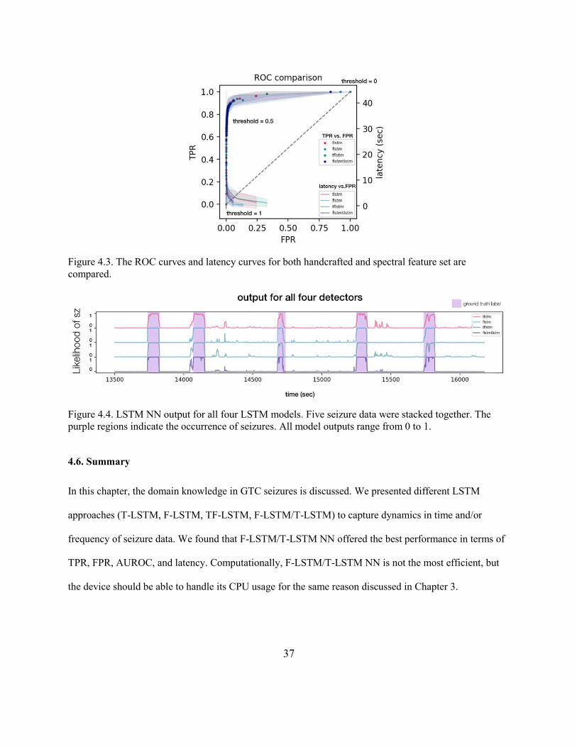
The ROC curves and latency curves show similar performance for all models (Figure 4.3). To further

examine on how each model performs, a fraction (5 seizures) of the model outputs are shown in Figure

4.4. T-LSTM NN is most susceptible to false alarms while F-LSTM NN looks closest to ground truth

label.

37

Figure 4.3. The ROC curves and latency curves for both handcrafted and spectral feature set are

compared.

Figure 4.4. LSTM NN output for all four LSTM models. Five seizure data were stacked together. The

purple regions indicate the occurrence of seizures. All model outputs range from 0 to 1.

4.6. Summary

In this chapter, the domain knowledge in GTC seizures is discussed. We presented different LSTM

approaches (T-LSTM, F-LSTM, TF-LSTM, F-LSTM/T-LSTM) to capture dynamics in time and/or

frequency of seizure data. We found that F-LSTM/T-LSTM NN offered the best performance in terms of

TPR, FPR, AUROC, and latency. Computationally, F-LSTM/T-LSTM NN is not the most efficient, but

the device should be able to handle its CPU usage for the same reason discussed in Chapter 3.

38

Chapter 5: Conclusion and future directions

5.1. Future direction

The future direction for this research project can span from open source collaboration, adaptation of new

sensors, to development of algorithm. Open source collaboration is highly encouraged since the scale of

EpiWatch research is growing as well as the team. A multi-center study for this project has just started,

which will invite more participants to contribute to the seizure data collection. As seizure data

accumulates, advanced algorithms that are only ideal for large dataset can now be developed. If the

preprocessing steps can be standardized, a lot of overhead work can be avoided. Secondly, we are also

interested in exploring the use of any available sensor on Apple Watch. Microphone is a particular

interest as patients experiencing GTCS can make a very characteristic sound: ictal cry. The snoring sound

they make once they enter the post-ictal suppression stage is a very characteristic sound pattern, which

can help extract advanced information that will be discussed in later section. On the other hand, the

speaker can be an effective tool to improve the efficacy of intervention. We envisioned EpiWatch

becoming the most recommended seizure detector. Not only we want to assist early intervention, we also

want to assess the severity of an epileptic patient. This can be done by evaluating the duration post-ictal

suppression of GTCS as it is shown to be an important risk factor for SUDEP. Finally, we believe the

seizure detector performance can be further improved by personalize the algorithm for each user type.

5.1.1. Build Python pip packages and unit tests for maintainability

In the EpiWatch team, we tried to standardized codes that are frequently used. However, this is done by

sharing the python files that contain these useful functions. These functions are still fluidic and subject to

changes, so there is a need for better methodology to develop and maintain these functions. Therefore, we

are interested in developing a python package for EpiWatch algorithm. Packaging of the python code can

be done easily through pip. On the other hand, unit tests are important as it help developers to track the

39

usability of their code without diving into the code. It makes the coding process more robust. It facilitates

changes and simplifies integration. It also provides documentation, which is missing a lot during the

development of isolation forest detector. It would be ideal to start this process before launching the

EpiWatch app with the seizure onset detector.

5.1.2. The use of microphone: detector targeted for ictal cry

The ictal cry was defined as a prolonged tonic expiratory laryngeal vocalization, or a deep guttural clonic

vocalization. It is strongly associated with epileptic GTCS and warrants inquiry when taking the history

from witnesses of a patient’s seizure (Elzawahry, Do, Lin, & Benbadis, 2010). Audio component of the

ictal cry is also very characteristic and similar across patients, making it a potential marker for seizure

onset detection. The utilization of microphone in EpiWatch app is expected to increase sensitivity and

lower FPR and latency for the detector.

5.1.3. The use of speaker: vocal instruction for timely intervention

When GTCS occur to patients, they could experience complications such as falling, suffocation, and loss

of conscience, which could danger patients’ lives in certain cases (e.g. GTCS while driving, swimming,

etc.). In these cases, care givers cannot reach the patients in time since the location of the incidents don’t

necessarily have to be close to the hospitals. It is important for people who are adjacent to the patients to

provide appropriate intervention. Simple interventions that can be instructed through vocal sound can be

very effective to prevent further serious complications such as drowning in swimming pool. Therefore,

the use of speaker for EpiWatch is of great interest to realize such need.

5.1.4. Evaluation of the duration of postictal generalized EEG suppression for better SUDEP risk

assessment

Postictal generalized EEG suppression (PGES) is a condition followed by the tonic-clone phase of a

convulsive seizure. PGES occurs more frequently after convulsive seizure arising from sleep. PGES thus

40

become an important biomarker for SUDEP since nocturnal convulsive seizure increase SUDEP risk

(Lamberts et al., 2013). A study has shown that PGES duration of greater than 20s following GTCS can

be a risk factor of SUDEP (Lhatoo et al., 2010). If EpiWatch can quantify PGES duration, it can be a risk

assessment tool in addition to its alerting capability, which helps improve epilepsy treatment strategy.

5.1.5. Personalized detector

The current seizure onset detector is trained on different patients. It is designed to generalize for GTCS

modeling capability for new patients. However, GTCS can have slightly different characteristics among

patients. Amplitude of a GTCS for an adult can be larger than that for a child. Although frequency and

time dynamics remain the same, the activation of the neurons in the LSTM NN can be different and

therefore, making the detector less sensitive, and less immediate. Therefore, we believe a personalized

detector can further improve detector performance on individuals. This task is very similar to speaker

adaptation using neural network. Specifically, this is essentially multi-task learning (a type of transfer

learning), where the source and target domains are different, but the source and target tasks are the same

(Pan & Yang, 2010). Most machine learning methods work well under the assumption that training and

testing data are drawn from the same feature space with the same distribution. Most models need to be

retrained when distribution changes. To prevent such overhead, transfer learning can be employed to

realize efficient domain adaptation. The training is done by first training the detector on GTCS from

different patients. It is then adapted to a specific patient by continuing the training process on GTCS of

that specific patient. Such NN converges much faster and does not overfit when compared to training on

only GTCS from that specific patient.

5.2. Conclusion

This paper has summarized work done by the author for EpiWatch project. It began with codebase

refactoring, in the form of a pipeline similar to Kaldi. The pipeline encourages collaboration and

41

improves maintainability. Within the framework of this pipeline, several research studies such as feature

set exploration and machine learning model architecture design can be performed efficiently. The two

feature sets explored, handcrafted features and spectral features, are fed into LSTM NN of similar

architectures for comparison. LSTM NN for spectral features outperformed handcrafted features in all

three metrics employed by the author. A more complicated LSTM NN has been designed and validated

based on the domain knowledge of GTCS. Different LSTM variants were implemented and the results

were compared using the same metrics. The F-LSTM/T-LSTM architecture author proposed helps

modeling both time and frequency dependencies, and therefore yields better performance. In the future,

we will continue to further solidify our codebase, explore the use of different sensors on Apple Watch,

assess duration of postictal suppression, and personalize the detector for better performance.

42

REFERENCES

Bass, N., Wyllie, E., Comair, Y., Kotagal, P., Ruggieri, P., & Holthausen, H. (1995). Supplementary

sensorimotor area seizures in children and adolescents. The Journal of Pediatrics, 126(4), 537–544.

https://doi.org/10.1016/S0022-3476(95)70346-2

Beniczky, S., Polster, T., Kjaer, T. W., & Hjalgrim, H. (2013). Detection of generalized tonic-clonic

seizures by a wireless wrist accelerometer: A prospective, multicenter study. Epilepsia, 54(4), e58–e61.

https://doi.org/10.1111/epi.12120

Bromfield, E. B., Cavazos, J. E., & Sirven, J. I. (2006). Basic Mechanisms Underlying Seizures and

Epilepsy. Retrieved from https://www.ncbi.nlm.nih.gov/books/NBK2510/

Chandrashekar, G., & Sahin, F. (2014). A survey on feature selection methods. Computers & Electrical

Engineering, 40(1), 16–28. https://doi.org/10.1016/j.compeleceng.2013.11.024

El-Amrawy, F., & Nounou, M. I. (2015). Are Currently Available Wearable Devices for Activity

Tracking and Heart Rate Monitoring Accurate, Precise, and Medically Beneficial? Healthcare

Informatics Research, 21(4), 315–320. https://doi.org/10.4258/hir.2015.21.4.315

Elzawahry, H., Do, C. S., Lin, K., & Benbadis, S. R. (2010). The diagnostic utility of the ictal cry.

Epilepsy & Behavior: E&B, 18(3), 306–307. https://doi.org/10.1016/j.yebeh.2010.04.041

Ficker, D. M., So, E. L., Shen, W. K., Annegers, J. F., O’Brien, P. C., Cascino, G. D., & Belau, P. G.

(1998). Population-based study of the incidence of sudden unexplained death in epilepsy. Neurology,

51(5), 1270–1274. https://doi.org/10.1212/WNL.51.5.1270

Ficker, & Ficker. (2000). Sudden unexplained death and injury in epilepsy. Epilepsia, 41(s2), S7–S12.

https://doi.org/10.1111/j.1528-1157.2000.tb01519.x

43

Lamberts, R. J., Gaitatzis, A., Sander, J. W., Elger, C. E., Surges, R., & Thijs, R. D. (2013). Postictal

generalized EEG suppression. Neurology, 81(14), 1252–1256.

https://doi.org/10.1212/WNL.0b013e3182a6cbeb

Lhatoo, S. D., Faulkner, H. J., Dembny, K., Trippick, K., Johnson, C., & Bird, J. M. (2010). An

electroclinical case-control study of sudden unexpected death in epilepsy. Annals of Neurology, 68(6),

787–796. https://doi.org/10.1002/ana.22101

Li, J., Mohamed, A., Zweig, G., & Gong, Y. (2015). LSTM time and frequency recurrence for automatic

speech recognition. 2015 IEEE Workshop on Automatic Speech Recognition and Understanding (ASRU),

187–191. https://doi.org/10.1109/ASRU.2015.7404793

Lugaresi, E., & Cirignotta, F. (1981). Hypnogenic Paroxysmal Dystonia: Epileptic Seizure or a New

Syndrome? Sleep, 4(2), 129–138. https://doi.org/10.1093/sleep/4.2.129

Mann, K. A., Wernere, F. W., & Palmer, A. K. (1989). Frequency spectrum analysis of wrist motion for

activities of daily living. Journal of Orthopaedic Research, 7(2), 304–306.

https://doi.org/10.1002/jor.1100070219

Nashef, L., Walker, F., Allen, P., Sander, J. W., Shorvon, S. D., & Fish, D. R. (1996). Apnoea and

bradycardia during epileptic seizures: relation to sudden death in epilepsy. Journal of Neurology,

Neurosurgery, and Psychiatry, 60(3), 297–300.

Pan, S. J., & Yang, Q. (2010). A Survey on Transfer Learning. IEEE Transactions on Knowledge and

Data Engineering, 22(10), 1345–1359. https://doi.org/10.1109/TKDE.2009.191

Poh, M.-Z., Loddenkemper, T., Reinsberger, C., Swenson, N. C., Goyal, S., Madsen, J. R., & Picard, R.

W. (2012). Autonomic changes with seizures correlate with postictal EEG suppression. Neurology,

78(23), 1868–1876. https://doi.org/10.1212/WNL.0b013e318258f7f1

44

Ryvlin, P., Nashef, L., Lhatoo, S. D., Bateman, L. M., Bird, J., Bleasel, A., … Tomson, T. (2013).

Incidence and mechanisms of cardiorespiratory arrests in epilepsy monitoring units (MORTEMUS): a

retrospective study. Lancet Neurol, 12(10), 966–977. https://doi.org/10.1016/S1474-4422(13)70214-X

Sainath, T. N., & Li, B. (2016, September 8). Modeling Time-Frequency Patterns with LSTM vs.

Convolutional Architectures for LVCSR Tasks. 813–817. https://doi.org/10.21437/Interspeech.2016-84

Tian, N. (2018). Active Epilepsy and Seizure Control in Adults — United States, 2013 and 2015. MMWR.

Morbidity and Mortality Weekly Report, 67. https://doi.org/10.15585/mmwr.mm6715a1

Tzallas, A. T., Tsipouras, M. G., Tsalikakis, D. G., Karvounis, E. C., Astrakas, L., Konitsiotis, S., &

Tzaphlidou, M. (2012). Automated Epileptic Seizure Detection Methods: A Review Study. Epilepsy -

Histological, Electroencephalographic and Psychological Aspects. https://doi.org/10.5772/31597

Van de Vel, A., Milosevic, M., Bonroy, B., Cuppens, K., Lagae, L., Vanrumste, B., … Ceulemans, B.

(2016). Long-term accelerometry-triggered video monitoring and detection of tonic–clonic and clonic

seizures in a home environment: Pilot study. Epilepsy & Behavior Case Reports, 5(Supplement C), 66–

71. https://doi.org/10.1016/j.ebcr.2016.03.005

Vandecasteele, K., De Cooman, T., Gu, Y., Cleeren, E., Claes, K., Paesschen, W. V., … Hunyadi, B.

(2017). Automated Epileptic Seizure Detection Based on Wearable ECG and PPG in a Hospital

Environment. Sensors, 17(10), 2338. https://doi.org/10.3390/s17102338

Yazdi, S., & Lashkari, Z. H. (n.d.). Technical analysis of Forex by MACD Indicator.

Zijlmans, M., Flanagan, D., & Gotman, J. (2002). Heart Rate Changes and ECG Abnormalities During

Epileptic Seizures: Prevalence and Definition of an Objective Clinical Sign. Epilepsia, 43(8), 847–854.

https://doi.org/10.1046/j.1528-1157.2002.37801.x

45

BIOGRAPHY

Michael Chan graduated from University of California, Los Angeles, with a Bachelor of Science degree

in Bioengineering. He conducted research under Dr. Wentai Liu’s guidance in his Biomimetic Research

Lab, where he built his favorite medical device: a noninvasive medical patch that captures both PPG and

ECG from the chest and streams to the mobile devices. Upon graduation, he joined Apple Inc. Health

Technologies Team as a biomedical R&D intern for 10 months, where he helped assess feasibility and

conduct studies for health hardware and applications of Apple Watch. He then entered Johns Hopkins

University as a Biomedical Engineering MSE student and has been a graduate researcher under Dr.

Nathan Crone’s guidance. His primary role for this research is to help progress the EpiWatch project by

utilizing various machine learning technique including neural network on the seizure onset detector. He is

still not satisfied with his accomplishments and knowledge in the field. To reach his goal, becoming a

bioengineer who can solve biomedical problems in the best possible way, he is resolved to continue his

academic journey through PhD.