Incorporating Saaty’s

Hierarchical Ranking Procedure

Into a Method for Locating

Serial Criminals

L. Carl Leinbach

Gettysburg College, USA

leinbach@gettysburg.edu

We will be exploring an interdisciplinary

subject that combines material from the

following areas and disciplines:

1.Matrix Algebra as a Method to

Quantify Individual‟s and/or

Society‟s Preferences

2. Social Psychology

3. Criminology

4. Geographic Profiling

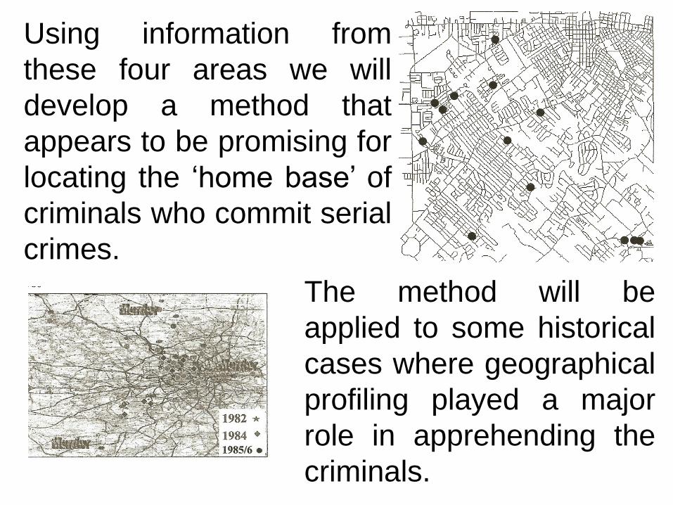
Using information from

these four areas we will

develop a method that

appears to be promising for

locating the „home base‟ of

criminals who commit serial

crimes.

The method will be

applied to some historical

cases where geographical

profiling played a major

role in apprehending the

criminals.

At the base of the method is a theorem by Perron and

Frobenius that states:

Every matrix having all positive values has an associated

dominant vector having all positive terms.

Obviously, this is beyond the scope of non university students.

However, the theorem can be easily illustrated if the students

have been introduced to matrices and vectors on the two

dimensional plane.

An example of a student activity using the Perron and

Frobenius result is available in the paper by P. Leinbach, C.

Leinbach, and J. Bőhm in Boletín #80 of Sociedad «Puig

Adam» De Profesores De Matematicas pp 23 -37

In the next few slides we will quickly show how this method is

applied to the problem at hand.

Our objective is to only illustrate what the action of a matrix of

all positive terms is when it is applied repeatedly to any

vector. This can easily be visualized in the plane.

Consider, for example, the matrix:

We will look at what happens when this matrix is applied to

the four corners of the square

given by the vectors

We will see that the square collapses to a straight line.

2

2

2

2

,

2

2

2

2

,

2

2

2

2

,

2

2

2

2

The result of the first multiplication is shown as the blue rectangle

superimposed on the original red square. Note that the rectangle

is now slanted in a particular direction and is a compressed form

of the original.

Next multiply the corner points of the blue rectangle by A or

doing the same thing by multiplying the corner points of the red

matrix by A2, we see a rectangle with a slightly different slant

and even more compressed. This rectangle is shown on the

next slide as a green rectangle.

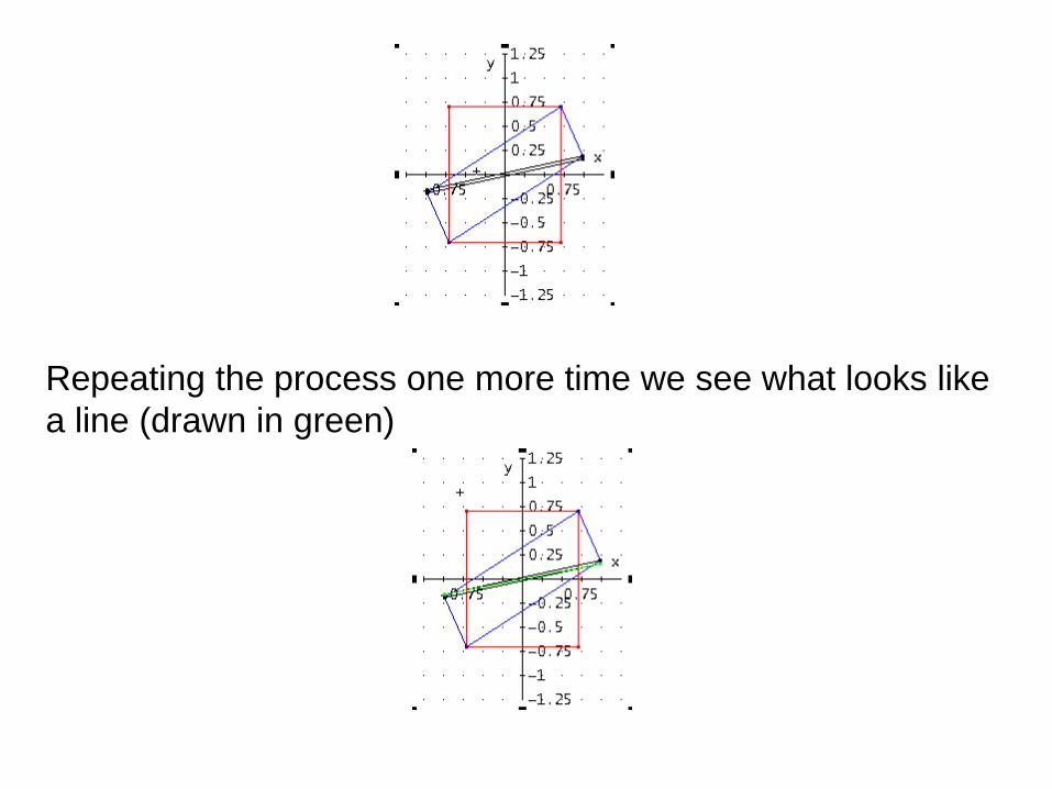
Repeating the process one more time we see what looks like

a line (drawn in green)

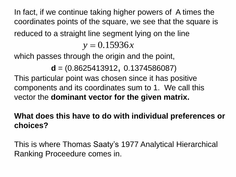
In fact, if we continue taking higher powers of A times the

coordinates points of the square, we see that the square is

reduced to a straight line segment lying on the line

which passes through the origin and the point,

d = (0.8625413912, 0.1374586087)

This particular point was chosen since it has positive

components and its coordinates sum to 1. We call this

vector the dominant vector for the given matrix.

What does this have to do with individual preferences or

choices?

This is where Thomas Saaty‟s 1977 Analytical Hierarchical

Ranking Proceedure comes in.

xy 15936.0

The basis of the AHRP is that generally people have no

trouble giving a strength of preference for one item over

another or quantizing the dominance of one entity over

another.

Humans have been doing it for years. Witness going to

the doctor‟s office: “On a scale of 1 to 10 rate your pain to

how you normally feel.” Or, in some of the more

sadistically oriented tests, “Rate this pain against the

previous pain you just experienced.”

Saaty very cleverly devised a method for creating a matrix

for a ranking between two choices to which he can apply

the Perron-Frobenius Theorem to create a vector which

gives a ranking of multiple choices and the strength of the

preference between these choices.

We consider the case of serial rapists.

Begin by categorizing different type of rapes:

I. Date Rape or Opportunistic Rape

II. Rape by more than one perpetrator

III. Use of a weapon in subduing victim

IV. Commission of a non-violent crime (burglary) at

time of rape.

V. Rape with bodily harm to victim

VI. Rape and murder of the victim

VII. Kidnapping or imprisonment and multiple rapes of

the victim.

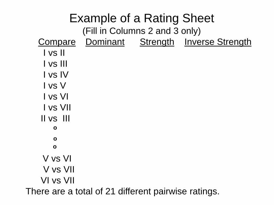
Example of a Rating Sheet(Fill in Columns 2 and 3 only)

Compare Dominant Strength Inverse Strength

I vs II

I vs III

I vs IV

I vs V

I vs VI

I vs VII

II vs IIIo

o

o

V vs VI

V vs VII

VI vs VII

There are a total of 21 different pairwise ratings.

How do we determine the value to put in column 3.

Saaty‟s guidelines are:

1 = no preference for one item over the other

3 = slightly stronger preference for one over the other

5 = an essential preference for one over the other

7 = some evidence that one is preferred over the other

9 = indisputable evidence for one over the other

Even numbers may be used if the evaluator is undecided

between two adjacent categories. A 10 is given if the

evidence is Overwhelming in the mind of the evaluator

Using the Rating Sheets, create a 7 X 7 matrix according to the

following rules:

A = (ai j) 1< i,j < 7

ai I = 1

If category j dominates category i with a preference of s,

ai j = s

else,

ai j = 1/s

The following matrix represents the consensus of a panel of „experts‟

for the seven categories of serial rape.

14/14891010

4139899

4/13/115568

8/19/15/11337

9/18/15/13/1116

10/19/16/13/1114

10/19/18/17/16/14/11

The following small Derive® 6.1 program finds the dominant vector (all

positive entries whose sum = 1) for the matrix related to the seven

categories of serial rape. The matrix is called “CM” for Consensus

Matrix.

Note that Category VI has the highest ranking (a little over 41%)

according to the consensus of the experts.

Geographic Profiling of Criminals

Described as: “An investigative support technique for

serial violent crime”

Developed at Simon Fraser University in Vancouver, BC,

Canada.

Primary work done by Kim Rossmo a student of Paul and

Patricia Brantingham at Simon Fraser

Rossmo spent several years as a constable on the

Vancouver Police force before attaining his Ph.D. at

Simon Fraser

Rossmo is now a private consultant and head of the

Center for Geospatial Intelligence and Investigation at

Texas State University, San Marcos, Texas

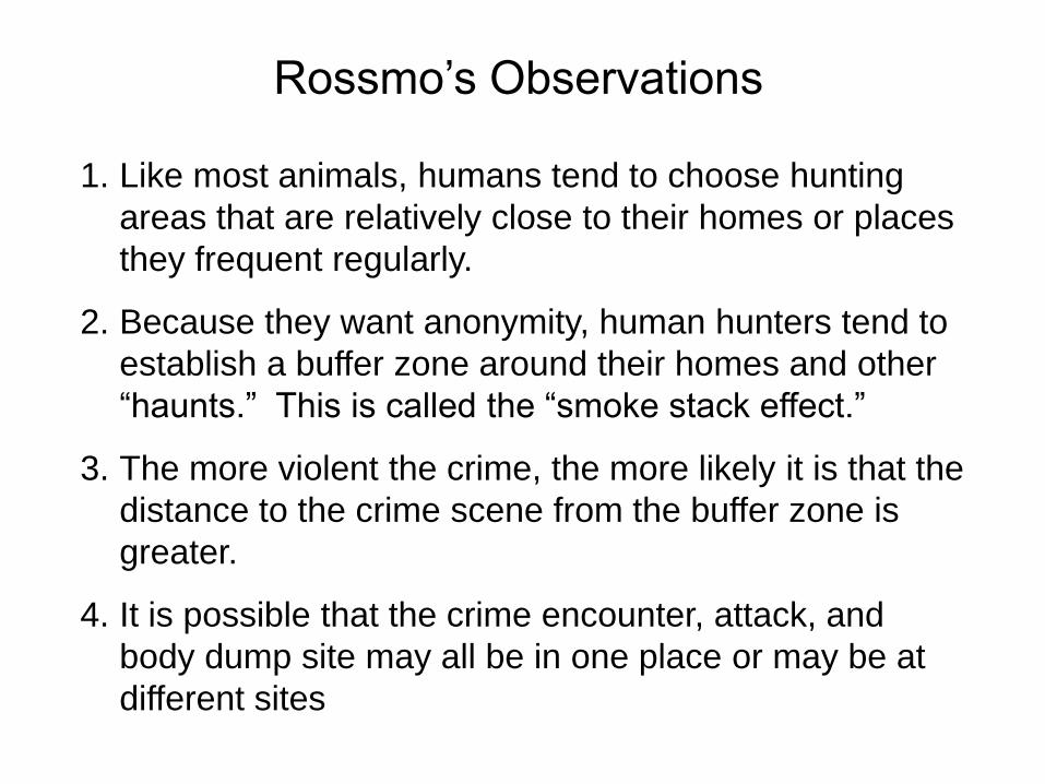
Rossmo‟s Observations

1. Like most animals, humans tend to choose hunting

areas that are relatively close to their homes or places

they frequent regularly.

2. Because they want anonymity, human hunters tend to

establish a buffer zone around their homes and other

“haunts.” This is called the “smoke stack effect.”

3. The more violent the crime, the more likely it is that the

distance to the crime scene from the buffer zone is

greater.

4. It is possible that the crime encounter, attack, and

body dump site may all be in one place or may be at

different sites

Rossmo‟s Insight

Rossmo‟s great insight was that the processes used for

making these observations could be reversed, i.e. it may

be possible to locate an area frequented by a serial

criminal from the locales of previous crime sites.

The main value of this is that it includes only a portion of

the hunting area and can make a significant reduction in

the number of suspects meeting the psychological

profile of the perpetrator of the serial crimes.

Rossmo uses a computer program, called Rigel after the

brightest star in the constellation Orion, the hunter.

The result is not an “X marks the spot,” but, rather, it

narrows down the area that most likely contains the

home, work area, or other location the perpetrator is

likely to frequent.

Rossmo‟s Procedure

1. Calculate the boundaries of the hunting area based on crime

locations.

2. For each point in the hunting area calculate the Manhattan or

“taxicab” distances to each crime scene.

3. Create a Pareto type function using distance to a crime scene as

an independent variable. If the distance is less than the radius of

the buffer zone, the function is reversed to minimize the

probability of that point being the criminals base. Do this for each

crime scene.

4. Sum the crime scene function values to produce a final score as

follows:

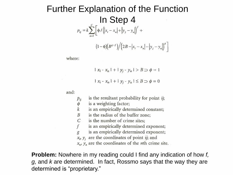
Further Explanation of the Function

In Step 4

Problem: Nowhere in my reading could I find any indication of how f,

g, and k are determined. In fact, Rossmo says that the way they are

determined is “proprietary.”

Bringing The AHRP and Geographic

Profiling Together

1. Point 3 of Rossmo‟s observations made brings to mind

using the AHRP generated dominant vector.

2. The dominant vector not only gives a ranking, but also

assigns a value to the strength of that ranking. For

example Category VI is viewed as about 2.7 times as

violent as Category V and Category VII is viewed as about

2 times as violent as Category 5 and 1½ times less violent

than Category VII.

3. The function ax for 0 < a < 1 decays in much the same way

as a Pareto function. NOTE: the larger a, the slower the

decay.

4. Some adjustment must be made for the Buffer Zone.

5. Use Derive®‟s ability to put pictures as background to

graphs to place crime scene location maps on the graph

and read off coordinates.

The Work of David Canter

David Canter a professor in the Centre for Investigative Psychology at the

University of Liverpool came into national prominence in the UK when he

helped the London Police narrow down the “home base” of the, then

unknown, “Railway Killer‟, John Duffy in 1986.

In a 2000 paper, Canter, and colleagues published a paper in the Journal

of Quantitative Criminology that examined the effectiveness of analytical

models of Geographical Profiling. In particular, they looked at models

based on the idea of a decay function of the form, . They

examined these functions for their statistical accuracy in know cases of

serial crimes.

While these functions represented the decay in the likely hood of the

criminal traveling from a particular distance to the crime scene, they did

not incorporate a buffer zone where it was less likely that the criminal

would commit the crime. The paper stated:

“To model the presence of a buffer zone, steps, areas with a B value

of 0, and plateaus of, areas of a constant B-value . . . , are inserted in

front of the exponential function.”

How I Approached the Problem

1. I basically liked Rossmo‟s insights and approach to the problem.

However, not knowing the values of f and g in his algorithm for

assigning a likely hood to points on the map left me against a stone

wall for proceeding.

2. Canter‟s exponential decay functions made a lot of sense to me for

assigning values to points outside of the buffer zone, but it did not

make sense to have a constant value inside the buffer zone.

Rossmo allowed for the (small) probabilityof an attack within this

zone.

3. The Brantingham‟s (Rossmo‟s thesis advisors at Simon Frazer) made

the observation that the serial perpetrator was, the further the

distance from the home base to the crime site.

4. Amalgamating these three points made me think of Saaty‟s AHRP

and using functions outside of the buffer zone of the form, ,

where β was related to a ranking of crime severity.

5. Inside of the buffer zone, I thought of using the reciprocal of 1 minus

the exponential that was scaled to have a value of 1 on the boundary

of the buffer zone.

I started in one dimension with a radius of 1 for the buffer zone by

graphing the DERIVE expression:

These curves have the shape that I am looking for inside the buffer

region, but need to be reflected about the line, y=x.

So, I solve for x in terms of y, and then interchange the roles of y and x

Outside of the buffer region, the curve will be a straight exponential

which equals 1 when x=B (δ in this function) and decays as x gets

further from B. The graph shows the resulting curves for x = 0.1, . . . ,0.9,

and δ = 2.5. I am only interested in the graph for positive x.

Pred(x, δ, β, α) ≔ Progα ≔ 1 - β

#5: If x ≤ δ ∧ β ≠ 1 LN(x·(α - 1)/δ + 1)/LN(α)β^(x/δ - 1)

The result has the type of shape that I am looking for.

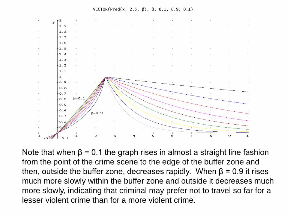
VECTOR(Pred(x, 2.5, β), β, 0.1, 0.9, 0.1)

Note that when β = 0.1 the graph rises in almost a straight line fashion

from the point of the crime scene to the edge of the buffer zone and

then, outside the buffer zone, decreases rapidly. When β = 0.9 it rises

much more slowly within the buffer zone and outside it decreases much

more slowly, indicating that criminal may prefer not to travel so far for a

lesser violent crime than for a more violent crime.

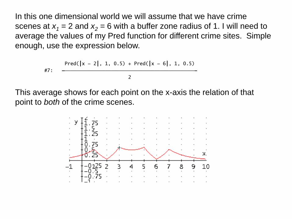
In this one dimensional world we will assume that we have crime

scenes at x1 = 2 and x2 = 6 with a buffer zone radius of 1. I will need to

average the values of my Pred function for different crime sites. Simple

enough, use the expression below.

Pred(⎮x - 2⎮, 1, 0.5) + Pred(⎮x - 6⎮, 1, 0.5) #7: ⎯⎯⎯⎯⎯⎯⎯⎯⎯⎯⎯⎯⎯⎯⎯⎯⎯⎯⎯⎯⎯⎯⎯⎯⎯⎯⎯⎯⎯⎯⎯⎯⎯⎯⎯⎯⎯⎯⎯⎯⎯⎯⎯⎯⎯

2

This average shows for each point on the x-axis the relation of that

point to both of the crime scenes.

The Case of John Duffy

We begin with the case that started it

all, it became known as the case of the

Railway Killer because of the three

murders in 1986. When Duffy started his

spree of serial rapes, it was thought that

there were 2 rapists. See photos to the

left. This threw the police off for some

time, but they finally connected the

earlier rapes that started in 1982 with

the 1986 rape/murders.

Professor David Cantor of Liverpool

University looked at the map to the left

and concentrating on Duffy‟s early

exploits and was able to find a

reasonable area for the police to look for

the perpetrator of all crimes.

Let‟s see how DERIVE, the AHRP, and I

do with the same information.

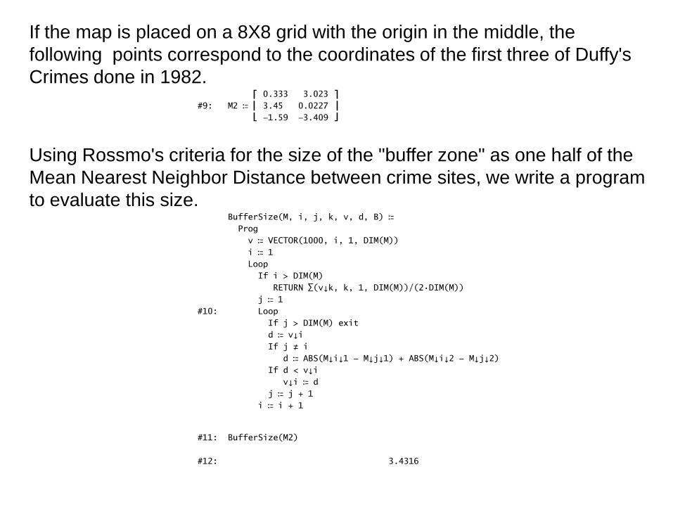
If the map is placed on a 8X8 grid with the origin in the middle, the

following points correspond to the coordinates of the first three of Duffy's

Crimes done in 1982. ⎡ 0.333 3.023 ⎤

#9: M2 ≔ ⎢ 3.45 0.0227 ⎥⎣ -1.59 -3.409 ⎦

Using Rossmo's criteria for the size of the "buffer zone" as one half of the

Mean Nearest Neighbor Distance between crime sites, we write a program

to evaluate this size.BufferSize(M, i, j, k, v, d, B) ≔ Progv ≔ VECTOR(1000, i, 1, DIM(M)) i ≔ 1 Loop If i > DIM(M)

RETURN ∑(v↓k, k, 1, DIM(M))/(2·DIM(M)) j ≔ 1

#10: Loop If j > DIM(M) exit d ≔ v↓iIf j ≠ i

d ≔ ABS(M↓i↓1 - M↓j↓1) + ABS(M↓i↓2 - M↓j↓2)If d < v↓i

v↓i ≔ d j ≔ j + 1

i ≔ i + 1

#11: BufferSize(M2)

#12: 3.4316

Given a point in the "hunting area" of the serial criminal, (x,y), we write a

function that is in the 'spirit' of Rossmo's function based on a Paereto

probability distribution, but using my Pred function. The parameter M is the

matrix of crime site locations, β is the normalized value for the 'intensity' of

this type of crime found using the AHRP, and δ is the buffer size. The

calculation uses the Manhattan Metric to determine distance.

Likelyhood(x, y, M, β, δ, i, j, d, p, s) ≔Progi ≔ 1 s ≔ 0 Loop

#13: If i > DIM(M) RETURN s/DIM(M)

d ≔ ABS(x - M↓i↓1) + ABS(y - M↓i↓2) p ≔ Pred(d, δ, β) s ≔ s + p i ≔ i + 1

We test the likely hood of two arbitrary points (0,0) and (-3.5,1.56) for crime

site locations in matrix, M2, β = 0.6, and δ = 3.05865. Note that (0,0) is a

rather likely candidate for the home base, and the second point is less likely.

#14: Likelyhood(0, 0, M2, 0.6, 3.05865)

#15: 0.8693155997#16: Likelyhood(-3.5, 1.56, M2, 0.6, 3.05865)

#17: 0.5401394059

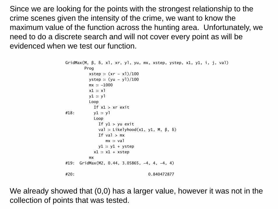
Since we are looking for the points with the strongest relationship to the

crime scenes given the intensity of the crime, we want to know the

maximum value of the function across the hunting area. Unfortunately, we

need to do a discrete search and will not cover every point as will be

evidenced when we test our function.

GridMax(M, β, δ, xl, xr, yl, yu, mx, xstep, ystep, x1, y1, i, j, val) Progxstep ≔ (xr - xl)/100 ystep ≔ (yu - yl)/100 mx ≔ -1000 x1 ≔ xl y1 ≔ ylLoop If x1 > xr exit

#18: y1 ≔ ylLoop If y1 > yu exit val ≔ Likelyhood(x1, y1, M, β, δ) If val > mx

mx ≔ valy1 ≔ y1 + ystep

x1 ≔ x1 + xstepmx

#19: GridMax(M2, 0.44, 3.05865, -4, 4, -4, 4)

#20: 0.840472877

We already showed that (0,0) has a larger value, however it was not in the

collection of points that was tested.

Let's get a 3-D view of the Likelyhood function for M2 with β = 0.44 and δ =

3.4316 showing those points where the likelyhood is above 95% of the

maximum value for the function.

#21: 0.95·0.840472877

#22: 0.7984492331

#23: Likelyhood(x, y, M2, 0.6, 3.4316)

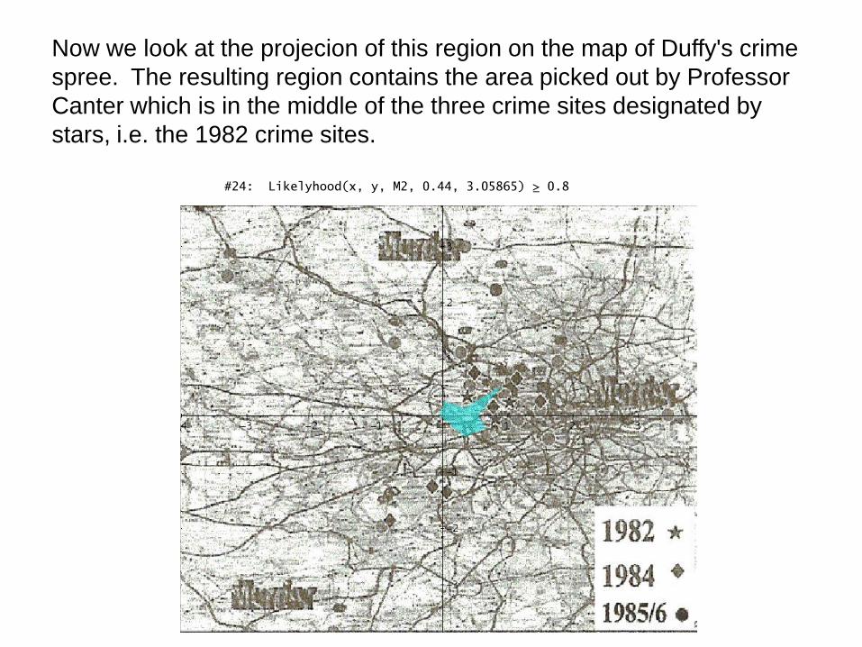
Now we look at the projecion of this region on the map of Duffy's crime

spree. The resulting region contains the area picked out by Professor

Canter which is in the middle of the three crime sites designated by

stars, i.e. the 1982 crime sites.

#24: Likelyhood(x, y, M2, 0.44, 3.05865) ≥ 0.8

The Derive® Working Environment And

The Lafayette, Louisana

South Side Rapist

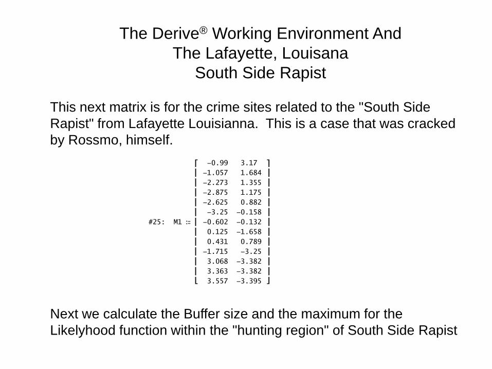
This next matrix is for the crime sites related to the "South Side

Rapist" from Lafayette Louisianna. This is a case that was cracked

by Rossmo, himself.

⎡ -0.99 3.17 ⎤⎢ -1.057 1.684 ⎥⎢ -2.273 1.355 ⎥⎢ -2.875 1.175 ⎥⎢ -2.625 0.882 ⎥⎢ -3.25 -0.158 ⎥

#25: M1 ≔ ⎢ -0.602 -0.132 ⎥⎢ 0.125 -1.658 ⎥⎢ 0.431 0.789 ⎥⎢ -1.715 -3.25 ⎥⎢ 3.068 -3.382 ⎥⎢ 3.363 -3.382 ⎥⎣ 3.557 -3.395 ⎦

Next we calculate the Buffer size and the maximum for the

Likelyhood function within the "hunting region" of South Side Rapist

#26: BufferSize(M1)

#27: 0.6512692307

#28: GridMax(M1, 0.44, 0.65127, -4, 4, -4, 4)

#29: 0.2525160807

Because this is such a small value, we will look at points that have a value of

60% of the maximum value of the Likelyhood function.

#30: 0.6·0.2525160807

#31: 0.1515096484

We now look at the 3D plot and the points that lie above 0.15.

#32: Likelyhood(x, y, M1, 0.44, 0.6512692307)

Projecting this region onto the map of the Rapist's hunting region in

Lafayette Louisiana, we get two areas that look promising. It turned out

that the rapist was a police detective who had moved from the area in the

upper left to the area in the lower right of the map during the crime spree.

#34: Likelyhood(x, y, M1, 0.44, 0.6512692307) ≥ 0.15

Jack the Ripper

Below are the regions (shown in red) selected as possibilities

for Jack‟s base of operations by Rossmo as illustrated in his

book.

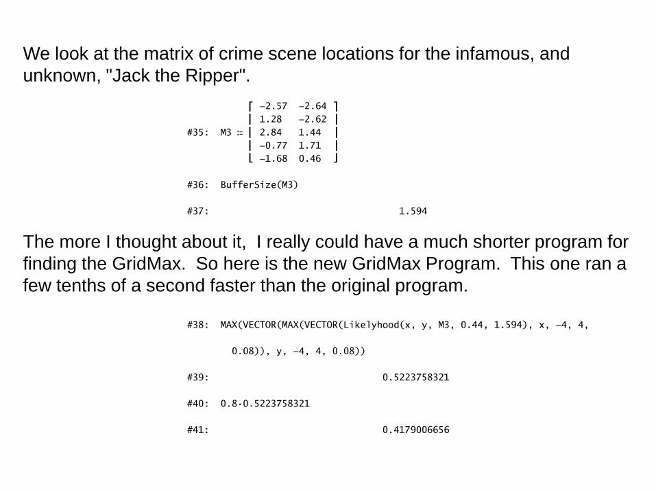
We look at the matrix of crime scene locations for the infamous, and

unknown, "Jack the Ripper".

⎡ -2.57 -2.64 ⎤⎢ 1.28 -2.62 ⎥

#35: M3 ≔ ⎢ 2.84 1.44 ⎥⎢ -0.77 1.71 ⎥⎣ -1.68 0.46 ⎦

#36: BufferSize(M3)

#37: 1.594

The more I thought about it, I really could have a much shorter program for

finding the GridMax. So here is the new GridMax Program. This one ran a

few tenths of a second faster than the original program.

#38: MAX(VECTOR(MAX(VECTOR(Likelyhood(x, y, M3, 0.44, 1.594), x, -4, 4,

0.08)), y, -4, 4, 0.08))

#39: 0.5223758321

#40: 0.8·0.5223758321

#41: 0.4179006656

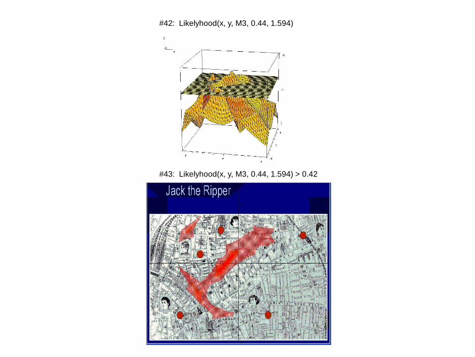
#42: Likelyhood(x, y, M3, 0.44, 1.594)

#43: Likelyhood(x, y, M3, 0.44, 1.594) > 0.42

Areas for Much More Research

1. I need to read more criminology research concerning buffer

zones and look at published numbers for different types of crimes.

2. The AHRP give values for β that are rather small. Is there a way

to maybe use Saaty‟s reasoning on comparisons to expand the

scale to β = 0.1, . . . , 0.9

3. Would it be better to adjust functions to scale of map and assign a

constant that will give a more reasonable rate of decay for the

exponential functions?

4. Is there a way that the AHRP can be used to determine Rossmo‟s

constants f, g, and k?

5. Rossmo‟s summing of probabilities represents a disjunction. I

think that Canter‟s idea of the average showing the “strength of a

relationship” makes much more sense. Does it?

6. Michael O‟Leary of Towson State University in Maryland and his

students developed a probability distribution for finding the home

base of serial criminals. This may be a promising direction.

Bibliography

1. Canter, David et al, “Predicting Serial Killers‟ Home

Base Using a Decision Support System”, Journal of

Quantitative Criminology, v 16, no 4, 2000 pp 457 - 478

2. Leinbach, Patricia y Carl, y Bőhm, Josef, “Directing Our

Suspicions (Using Matrix Algebra to organize the results

of an investigation)” , Boletín N.o 80 Sociedad «Puig

Adam» De Profesores De Matematicas , Ocober, 2008,

pp 23 – 37

3. O'Leary, Mike, “The Mathematics of Geographic

Profiling”, Journal of Investigative Psychology and

Offender Profiling, v 6, 2009, pp. 253-265

4. Rossmo, D. Kim, Geographic Profiling, CRC Press,

Bocca Raton, Florida, 2000