Graduate Theses and Dissertations Iowa State University Capstones, Theses andDissertations

2011

Incorporating uncertainty in vehicle miles traveledprojections of the National Energy ModelingSystemDavid Michael PoettingIowa State University

Follow this and additional works at: https://lib.dr.iastate.edu/etd

Part of the Mechanical Engineering Commons

This Thesis is brought to you for free and open access by the Iowa State University Capstones, Theses and Dissertations at Iowa State University DigitalRepository. It has been accepted for inclusion in Graduate Theses and Dissertations by an authorized administrator of Iowa State University DigitalRepository. For more information, please contact digirep@iastate.edu.

Recommended CitationPoetting, David Michael, "Incorporating uncertainty in vehicle miles traveled projections of the National Energy Modeling System"(2011). Graduate Theses and Dissertations. 12129.https://lib.dr.iastate.edu/etd/12129

Incorporating uncertainty in vehicle miles traveled projections

of the National Energy Modeling System

by

David Michael Poetting

A thesis submitted to the graduate faculty

in partial fulfillment of the requirements for the degree of

MASTER OF SCIENCE

Major: Mechanical Engineering

Program of Study Committee:

W. Ross Morrow, Major Professor

Baskar Ganapathysubramanian

James Bushnell

Iowa State University

Ames, Iowa

2011

Copyright © David Michael Poetting, 2011. All rights reserved.

ii

TABLE OF CONTENTS

LIST OF FIGURES ................................................................................................................. iv

LIST OF TABLES .................................................................................................................... v

LIST OF NOMENCLATURE ................................................................................................. vi

ACKNOWLEDGEMENTS .................................................................................................... vii

ABSTRACT ........................................................................................................................... viii

CHAPTER 1: INTRODUCTION ............................................................................................. 1 1.1 Background ............................................................................................................. 1

1.2 Motivation ............................................................................................................... 2 1.3 Objective ................................................................................................................. 4

CHAPTER 2: ESTIMATING THE VMT MODEL ................................................................ 6 2.1 Introduction ............................................................................................................. 6 2.2 The VMT Model ..................................................................................................... 8

2.3 Cochrane-Orcutt .................................................................................................... 10 2.4 Maximum Likelihood ........................................................................................... 11

2.5 Prais-Winsten ........................................................................................................ 13 2.6 Results ................................................................................................................... 16

CHAPTER 3: MODELING THE UNCERTAINTY IN VMT............................................... 18

3.1 Introduction ........................................................................................................... 18 3.2 Monte Carlo Simulation of VMT Trajectories ..................................................... 19

3.3 Results ................................................................................................................... 20

CHAPTER 4: DECISION-MAKING ..................................................................................... 25

4.1 Introduction ........................................................................................................... 25 4.2 The VMT Model ................................................................................................... 26 4.3 Deterministic ......................................................................................................... 28 4.4 Expected Value ..................................................................................................... 29 4.5 Markovian ............................................................................................................. 29

4.6 Probabilistic .......................................................................................................... 30 4.7 Results ................................................................................................................... 32

CHAPTER 5: CONCLUSION ............................................................................................... 38 5.1 Summary ............................................................................................................... 38 5.2 Future Work .......................................................................................................... 40

iii

APPENDIX A: VMT MODEL FOR PRAIS-WINSTEN ESTIMATION ............................. 41

APPENDIX B: VMT MODEL FOR DECISION-MAKING ANALYSIS ............................ 43

APPENDIX C: THE PROBABILISTIC VMT MODEL ....................................................... 45

REFERENCES ....................................................................................................................... 48

iv

LIST OF FIGURES

Figure 1: VMT trajectories with uncertainty in the parameters and error term. ..................... 21

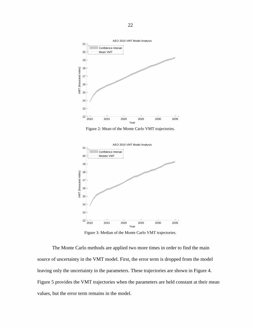
Figure 2: Mean of the Monte Carlo VMT trajectories. ........................................................... 22

Figure 3: Median of the Monte Carlo VMT trajectories......................................................... 22

Figure 4: VMT trajectories with uncertainty only in the parameters...................................... 23

Figure 5: VMT trajectories with uncertainty only in the error term. ...................................... 23

Figure 6: Projections of uncertain VMT with a fuel tax. ........................................................ 33

Figure 7: PDFs of VMT in 2020. ............................................................................................ 33

Figure 8: Mean and median VMT. ......................................................................................... 34

Figure 9: Projections of fuel consumption per licensed driver. .............................................. 35

Figure 10: Projections of fuel consumption by all US drivers................................................ 35

Figure 11: Projections of the fuel tax required to reduce VMT to the target.......................... 36

Figure 12: Projections of the total fuel tax paid each year per licensed driver. ...................... 36

v

LIST OF TABLES

Table 1: Historical data for the inputs of the VMT equation. ................................................... 7

Table 2: Parameter estimates and standard errors from three estimation techniques. ............ 16

Table 3: Projections for the VMT inputs used in the Mont Carlo simulation. ....................... 19

Table 4: Projections for the VMT inputs used in the decision-making analysis. ................... 26

vi

LIST OF NOMENCLATURE

fuel cost of driving one mile 2000 cents per mile

log

fuel economy miles per gallon

target for vehicle miles traveled per licensed driver thousand miles

per capita disposable personal income 2000 do

C

c C

E

G

I

llars

log

deterministic vehicle miles traveled per licensed driver thousand miles

probabilistic vehicle miles traveled per licensed driver thousand miles

Markovian vehicle miles traveled per license

i I

M

M

M

2

*

d driver thousand miles

log

normal random variable with mean 0 and variance

weighted summation of all previous normal random variables

fuel price 2000 cents per gallon

fuel tax 2000 cents per

m M

N

N N

P

T

0

0

gallon

vector of inputs 1

total number of years projected

subscript indicating year

vector of betas

coefficient for constant term

coefficient for cost of driving

coefficient for inco

T

M I C

C

I

x m i c

Y

y

2

* *

me

coefficient for vehicle miles traveled

serially correlated errors of AR 1 model

autocorrelation coefficient of AR 1 model

standard error variance of

standard error of

degree of certainty fo

M

N

N

r probabilistic decision making

EIA Energy Information Administration

GHG greenhouse gas

NEMS National Energy Modeling System

VMT vehicle miles traveled per licensed driver

vii

ACKNOWLEDGEMENTS

I am very grateful for the opportunity to work on this project and the academic and

personal growth I have gained from it. I was fortunate to have Ross Morrow as my major

professor. I have enjoyed working with Dr. Morrow, whose advice, guidance, and patience

has helped me become a much better student and researcher the last two years.

I want to thank my committee members Baskar Ganapathysubramanian and Jim

Bushnell for taking the time to review and discuss my research. Their advice and comments

are greatly appreciated. I would also like to acknowledge Dan Nordman, who was always

happy to meet with me and answer any questions I might have.

A heartfelt thank you goes out to my parents Gary and Kathy Poetting. All of my

accomplishments in life are a result of their endless love, support, and belief in me. Lastly, I

want to thank my fiancée Masse Carr. This thesis would not have been possible without your

love, encouragement, and patience. I cannot possibly thank you enough for everything you

have done for me.

viii

ABSTRACT

The National Energy Modeling System (NEMS) is a computational model that

forecasts the production, consumption, and prices of energy in the United States. Although

NEMS is a complex and detailed model, it does not currently represent the multitude of

uncertainties associated with the US energy system. These uncertainties need to be

communicated to policy makers in order for them to develop better-informed decisions

regarding energy policy. In this study, uncertainty is added to the vehicle miles traveled

(VMT) equation of NEMS to demonstrate the importance and benefit of uncertainty in the

model. The VMT model is derived and its uncertain parameters are estimated using

maximum likelihood estimation. A Monte Carlo simulation is performed to model the

uncertain VMT equation and demonstrate the range of possible VMT forecasts when these

uncertainties are included. This simulation shows that the deterministic forecast does not

adequately reflect all of the possible futures of VMT, which could lead policy makers to be

unintentionally misinformed about the impacts of proposed policies. Finally, it is shown how

the uncertain VMT equation could be used to help policy makers decide on the best policy to

reduce transportation greenhouse gas emissions. A target is set for VMT for each of the

projected years, and four decision-making techniques are used to calculate the fuel tax

required to reduce VMT to this specified goal. These methods could guide policy makers to

better-informed energy policy decisions, but they are only possible if some amount of

uncertainty is incorporated into the model.

1

CHAPTER 1: INTRODUCTION

1.1 Background

Energy forecasts are commonly used in the United States to predict energy use up to

25 years in the future. They provide the foundation for the energy industry, and play a vital

role in the formation of energy and environmental policy. Energy forecasts inspire research

in energy production and conversion, warn of environmental impacts such as climate change

and air pollution, and suggest the need for energy and environmental policy.

The Energy Information Administration (EIA) of the US Department of Energy has

been publishing energy forecasts in their Annual Energy Outlook (AEO) for nearly thirty

years (EIA, 2010a). In 1982, the EIA started using the Intermediate Future Forecasting

System (IFFS) to make energy predictions. The National Energy Modeling System (NEMS)

replaced the IFFS model in 1994 (EIA, 2010b). NEMS is a computer based energy-economy

modeling system that forecasts the production, consumption, conversion, and prices of

energy in the United States (EIA, 2009). It is designed to model the complex interactions of

supply and demand in US energy markets (Gabriel, Kydes, & Whitman, 2001). NEMS is

used by the EIA to gain insight on the impact of energy policies and different economic

assumptions.

NEMS is organized into a modular structure due to the diversity of energy markets.

The model consists of four end-use demand modules, four supply modules, two conversion

modules, one economic module, one international module, and a module that finds the

market equilibrium across all the NEMS modules (EIA, 2009). The modularity of NEMS

2

allows for each sector of the US energy system to use the procedures and techniques best

suited for that particular module. Each module is also divided geographically. NEMS is a

regional model because supply, demand, and other characteristics of the energy system vary

widely across the United States. Projections in the AEO 2010 span from the present to the

year 2035. The EIA believes technology, demographics, and economic conditions are

understood well enough to sufficiently represent the US energy market in this time period.

1.2 Motivation

The EIA’s projections have a significant influence on energy policy, making it

important to analyze the accuracy of NEMS. Evaluating the performance of previous energy

projections can provide insight into the possible errors connected to current projections. Error

analyses also direct researchers toward the cause of such errors, which could lead to

improvements in the model. Studies agree that NEMS has repeatedly underestimated total

energy consumption (Fischer, Herrnstadt, & Morgenstern, 2009; O'Neill & Desai, 2005;

Winebrake & Sakva, 2006). Fischer, Herrnstadt, and Morgenstern (2009) and Winebrake and

Sakva (2006) argue that it is misleading to judge the accuracy of energy projections by the

error in total energy demand, and the errors need to be broken down to the different sectors

modeled by NEMS. This approach shows that low errors for the total energy consumption

are hiding much higher errors in the individual sectors, which tend to cancel each other out

when combined. In addition, O’Neill & Desai (2005) find no evidence that suggests the

accuracy of these forecasts has improved since the EIA first began making energy

projections.

3

The limitations of energy forecasts need to be communicated to the policy makers

who rely heavily on their results to make informed policy decisions. The EIA attempts to

address this by forecasting five different scenarios: a reference case, high economic growth

case, low economic growth case, high oil price case, and low oil price case (EIA, 2009).

However, these five cases do not account for the myriad of uncertainties that lie within the

US energy system. In their research on long-term policy analysis Lempert, Popper, and

Bankes (2003) suggest hundreds to millions of scenarios are needed to span the range of

plausible outcomes in order to find the most robust policy strategy. This type of

comprehensive scenario analysis is not a practical method for a model as complex as NEMS.

Forecasts such as NEMS depend significantly on a variety of economic assumptions,

future oil prices, consumer preferences and behaviors, new technologies yet to be developed,

and numerous other inputs which are impossible to predict and inherently uncertain. If

NEMS inputs are uncertain, then NEMS forecasts must be uncertain as well. Baghelai,

Moumen, Cohen, Kydes, and Harris (1995a; 1995b) discuss techniques for characterizing the

uncertainty in NEMS, though very little has been done to put these methods to practice.

Without explicitly including uncertainties in forecasts, policy makers can be unintentionally

misinformed about the impacts of proposed policies. It is important to understand that no

forecasting model, no matter how complex, can exactly predict the future of the US energy

system. However, including uncertainty in NEMS forecasts would at least allow policy

makers to develop better-informed decisions regarding energy policy.

4

1.3 Objective

It is no secret that the world is going through a climate change, largely due to

increased emissions of greenhouse gases (GHG). Transportation sources contribute nearly a

third of the total US GHG emissions, and are responsible for half of the net increase in total

US emissions since 1990. Transportation is also the largest source of carbon dioxide (CO2)

emissions, which is the most notorious greenhouse gas (EPA, 2010). Reducing CO2

emissions from the transportation industry is a vital part of United States’ efforts to mitigate

the effect of greenhouse gases on global climate change.

Since transportation is the fastest growing source of GHG emissions, it also presents

the potential to be a leading source of GHG reductions. Several studies have been done to

determine the best policy strategies to reduce GHG emissions in the transportation sector

(DeCicco & Mark, 1998; Greene & Plotkin, 2001; McCollum & Yang, 2009; Morrow,

Gallagher, Collantes, & Lee, 2010). Based on an analysis using three scenarios of future

transportation energy use, Greene and Plotkin (2001) conclude GHG emissions would

continue to rise without dramatic increases in fuel prices. Although increasing the Corporate

Average Fuel Economy standards and using low carbon fuels slow this growth, these

strategies require some time to affect emissions due to the slow turnover of the vehicle fleet

and the slow rate of new technology development. According to McCollum and Yang

(2009), a combination of these policy scenarios are needed to make significant cuts to

transportation emissions. However, slowing the growth in vehicle miles traveled (VMT) is

the most effective way to decrease GHG emissions, and increasing the cost of driving with a

fuel tax is the only strategy that could significantly reduce VMT (Morrow et al., 2010).

5

The EIA includes projections of VMT in the Transportation Sector Module of NEMS.

While the main purpose of the Transportation Module is to project transportation energy

demand by fuel type, it also estimates vehicle stock, energy efficiency of vehicles,

deployment of new transportation technologies, and vehicle miles traveled (EIA, 2010c). The

module is divided into four modules representing different modes of travel: light-duty

vehicle, air travel, freight transport, and miscellaneous energy demand. Within the Light-

Duty Vehicle Module is the VMT Submodule, which generates a projection of the demand

for personal travel.

The purpose of this research is to incorporate uncertainty in the VMT model of

NEMS in order to help policy makers formulate better-informed decisions regarding

transportation energy policy. This starts by deriving the model and estimating its parameters

and their corresponding standard errors. Three estimation techniques are applied in order to

find the most appropriate estimation method. A Monte Carlo simulation is performed to

demonstrate the variety of VMT projections possible when uncertainty is included in the

model. Four methods are then used to determine a fuel tax that would increase the cost of

driving, thus decreasing vehicle miles traveled and CO2 emissions.

6

CHAPTER 2: ESTIMATING THE VMT MODEL

2.1 Introduction

The first step in developing an uncertain VMT model is deriving the model and

estimating its parameters. The goal is to incorporate uncertainty in the existing VMT model

without changing the structure of the model itself. Therefore, the uncertain model will look

the same as the VMT model currently used by NEMS, with the addition of an error term.

Parameter estimation is based on historical data for each of the inputs. The EIA does

not explicitly state which historical data was used when estimating the parameters for their

model. The historical data used in this parameter estimation was compiled from various

tables published by the Federal Highway Administration (FHWA, 2010) and the Bureau of

Economic Analysis (BEA, 2009). The most accurate, reliable, and comprehensive historical

data available is used here. However, this data is likely different from the data used by the

EIA, which results in different parameter estimates. The historical data used for the inputs is

given in Table 1.

Greene (2008) explains several methods that can be used to estimate the parameters

of a time series model. All of the estimation methods covered in this chapter are programmed

using MATLAB. LeSage (1999) describes how MATLAB can be used to implement various

econometric estimation techniques. In order to find the most appropriate estimation method,

three different techniques are applied to the VMT model: Cochrane-Orcutt, maximum

likelihood, and Prais-Winsten. This chapter describes each of these procedures and compares

their results to discover the preferred method.

7

year

vehicle miles

traveled per

licensed driver

(thousand miles)

per capita

disposable

personal income

(2000 dollars)

fuel cost of

driving 1 mile

(2000 cents/mile)

1966 8.603 11,827.39 10.27

1967 8.770 12,149.87 10.27

1968 9.042 12,532.69 10.29

1969 9.203 12,756.51 10.28

1970 9.350 13,072.67 10.09

1971 9.681 13,397.91 9.58

1972 9.985 13,779.33 9.24

1973 10.103 14,552.71 9.53

1974 9.531 14,483.48 11.66

1975 9.556 14,518.74 11.33

1976 9.774 14,917.30 11.16

1977 9.891 15,296.19 10.82

1978 10.175 15,842.36 10.45

1979 9.870 16,116.53 12.76

1980 9.723 16,325.56 15.07

1981 9.793 16,508.97 14.80

1982 9.836 16,621.71 12.75

1983 9.919 17,074.43 11.67

1984 10.255 18,142.93 10.77

1985 10.498 18,587.13 10.39

1986 10.681 19,071.14 7.88

1987 11.015 19,362.62 7.67

1988 11.559 20,122.50 7.17

1989 11.767 20,573.53 7.45

1990 11.929 20,877.18 7.92

1991 11.934 20,788.65 7.25

1992 12.061 21,354.14 7.03

1993 12.304 21,428.54 6.85

1994 12.434 21,839.89 6.68

1995 12.672 22,255.25 6.67

1996 12.790 22,783.76 7.00

1997 12.935 23,332.02 6.84

1998 13.126 24,397.08 5.85

1999 13.254 24,883.44 6.35

2000 13.292 25,944.00 7.77

2001 13.495 26,212.72 7.38

2002 13.557 26,751.54 6.89

2003 13.589 27,135.78 7.91

2004 13.762 27,744.67 8.93

2005 13.762 27,762.47 10.26

2006 13.732 28,465.56 11.06

2007 13.601 28,748.06 11.60

2008 13.148 28,968.01 13.17

Table 1: Historical data for the inputs of the VMT equation.

8

2.2 The VMT Model

The factors that affect vehicle miles traveled per licensed driver in year y yM are

the VMT from the previous year 1yM , per capita disposable personal income yI , and

the fuel cost of driving one mile yC . The natural logarithm of each of these inputs is taken

before inserting them into the model. To condense the notation, let the lowercase inputs

represent the natural logarithm of the actual inputs.

log

log

log

y y

y y

y y

m M

i I

c C

(2.1)

These inputs, along with their corresponding unknown parameters , create the time series

model given below.

0 1y M y I y C y ym m i c (2.2)

The EIA assumes this is a first order autoregressive, or AR(1), model. More

complicated processes are sometimes difficult to analyze and unnecessarily complex for this

research. The model should stay simple enough for policy makers to understand. The AR(1)

model is a convenient yet reasonable model to start with when the actual time series model is

unknown (Greene, 2008). An AR(1) model is defined by its serially correlated errors,

1

1 1

y y yN

(2.3)

with the assumption that 2Normal 0,yN .

9

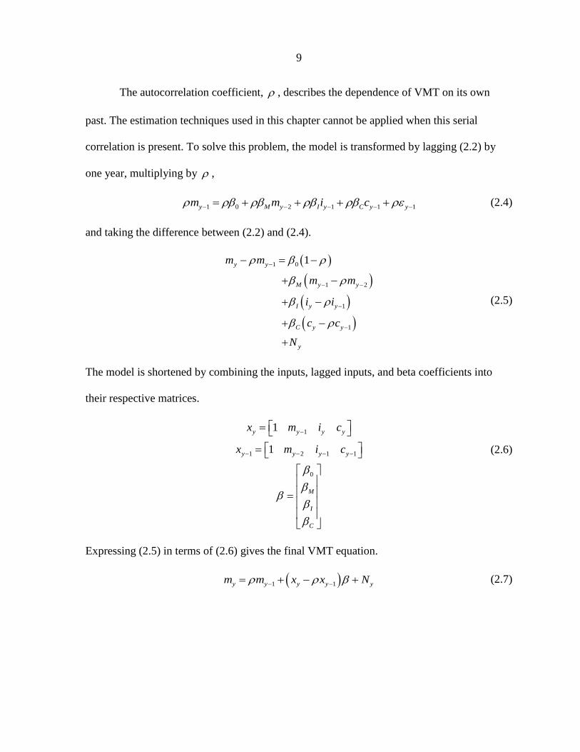
The autocorrelation coefficient, , describes the dependence of VMT on its own

past. The estimation techniques used in this chapter cannot be applied when this serial

correlation is present. To solve this problem, the model is transformed by lagging (2.2) by

one year, multiplying by ,

1 0 2 1 1 1y M y I y C y ym m i c (2.4)

and taking the difference between (2.2) and (2.4).

1 0

1 2

1

1

1y y

M y y

I y y

C y y

y

m m

m m

i i

c c

N

(2.5)

The model is shortened by combining the inputs, lagged inputs, and beta coefficients into

their respective matrices.

1

1 2 1 1

0

1

1

y y y y

y y y y

M

I

C

x m i c

x m i c

(2.6)

Expressing (2.5) in terms of (2.6) gives the final VMT equation.

1 1y y y y ym m x x N (2.7)

10

2.3 Cochrane-Orcutt

The Cochrane-Orcutt procedure (Cochrane & Orcutt, 1949) has been used to calculate

VMT since NEMS was first ran in 1994. The iterative process begins by choosing a starting

value for such as 0 . This value for is used to calculate the starred variables below.

*

1

*

1

y y y

y y y

m m m

x x x

(2.8)

Equation (2.7) is rewritten in terms of (2.8), and the normal error term is dropped.

* *

y ym x (2.9)

An ordinary least squares regression is ran on (2.9) to get an estimate for . Then (2.2) and

the estimated are used to calculate the errors and lagged errors.

1 1 1

y y y

y y y

m x

m x

(2.10)

A second ordinary least squares regression is done to estimate the correlation coefficient.

1y y (2.11)

This completes the first iteration, and the new estimate for is used in (2.8) to start the

second iteration. The procedure continues until two successive estimates for differ by less

than some predetermined value. The final is then used calculate the final estimate for .

11

2.4 Maximum Likelihood

Next, maximum likelihood estimation is used to estimate the parameters of the model.

As with all maximum likelihood estimation, this begins with calculating the likelihood

function.

1 2 1 2

1

, , ,Y

Y Y y

y

L f m m m f m f m f m f m

(2.12)

Using the fact that 2Normal 0,yN the distribution of ym is calculated to be

2

22

2

1

2

yF

yf m e

(2.13)

where

1 1,y y y y yF F m m x x (2.14)

When attempting to maximize the likelihood function it is often computationally easier to

minimize the negative log-likelihood function. Substituting (2.13) into (2.12) and taking the

negative logarithm yields

1

2

21

log log

1log 2 log

2 2

Y

y

y

Y

y

y

L f m

YY F

(2.15)

The first derivative of (2.15) with respect to is

2

21

log 1 1 Y

y

y

LY F

(2.16)

Since 0, , the 1 factor in front can be dropped when solving log 0L .

12

2

1

log 10

Y

y

y

LF

Y

(2.17)

The partial derivatives of (2.15) with respect to the rest of the parameters are given below.

1 121

210

2 121

121

12

log 1

log 11

log 1

log 1

log 1

Y

y y y

y

Y

y

y

Y

y y y

yM

Y

y y y

yI

y y y

C

LF x m

LF

LF m m

LF i i

LF c c

1

Y

y

(2.18)

Just as before, the 21 factor cannot force the partial derivatives in (2.18) to equal zero.

Dropping this term from (2.18) gives the conditions which must be satisfied in order for the

negative log-likelihood function to be minimized.

1 1

1

10

2 1

1

1

1

1

1

log0 0

log0 1 0

log0 0

log0 0

log0 0

Y

y y y

y

Y

y

y

Y

y y y

yM

Y

y y y

yI

Y

y y y

yC

LF x m

LF

LF m m

LF i i

LF c c

(2.19)

Finding the parameters that satisfy (2.19) simplifies to minimizing the following function.

13

2

1

1

2

Y

y

y

F

(2.20)

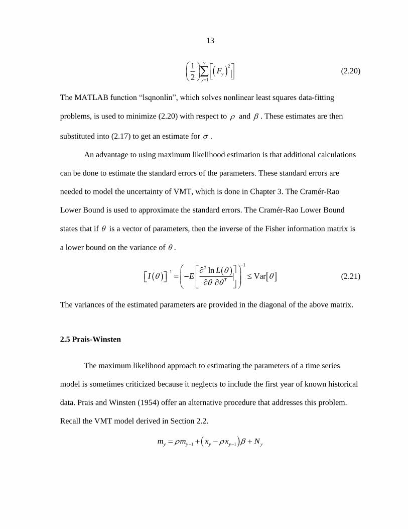
The MATLAB function “lsqnonlin”, which solves nonlinear least squares data-fitting

problems, is used to minimize (2.20) with respect to and . These estimates are then

substituted into (2.17) to get an estimate for .

An advantage to using maximum likelihood estimation is that additional calculations

can be done to estimate the standard errors of the parameters. These standard errors are

needed to model the uncertainty of VMT, which is done in Chapter 3. The Cramér-Rao

Lower Bound is used to approximate the standard errors. The Cramér-Rao Lower Bound

states that if is a vector of parameters, then the inverse of the Fisher information matrix is

a lower bound on the variance of .

12

1 lnVar

T

LI E

(2.21)

The variances of the estimated parameters are provided in the diagonal of the above matrix.

2.5 Prais-Winsten

The maximum likelihood approach to estimating the parameters of a time series

model is sometimes criticized because it neglects to include the first year of known historical

data. Prais and Winsten (1954) offer an alternative procedure that addresses this problem.

Recall the VMT model derived in Section 2.2.

1 1y y y y ym m x x N

14

The Prais-Winsten procedure uses a different model for the first year of data, thus one more

year of the historical data can be utilized. The model for the first year of data is explained in

Appendix A.

11 1

2

1 1

1

2,3,...,y y y y y

Nm x

m m x x N y Y

(2.22)

Estimating the parameters of this model is more complicated than the maximum likelihood

procedure due to the transformed model for the first year, but it essentially requires the same

steps. The process starts by calculating the distribution of ym .

221 1

2

2

2

12

21 2

2

2

1

2

1 2,3,...,

2

y

m x

F

y

f m e

f m e y Y

(2.23)

These distributions are used to calculate the negative log-likelihood function.

1

2

2

22

1 12

2

22

log log log

1log 2 log log 1

2 2

1 1

2

1

2

Y

y

y

Y

y

y

L f m f m

YY

m x

F

(2.24)

Again, the negative log-likelihood function is minimized by setting each of its partial

derivatives equal to zero and simplifying.

15

222

1 1

2

1log

0

Y

y

y

m x FL

Y

(2.25)

22

1 1 1 122

2

1 1

20

2

0 1 1 2 1

2

2

1 1 1 1

log0 0

1

log0 1 1 0

log0 1 0

log0 1

Y

y y y

y

Y

y

y

Y

y y y

yM

y y y

I

Lm x F x m

Lm x F

Lm m x F m m

Li m x F i i

2

2

1 1 1 1

2

0

log0 1 0

Y

y

Y

y y y

yC

Lc m x F c c

(2.26)

Solving the above system of equations does not simplify to the minimization of a less

complicated equation, as is the case with the maximum likelihood method. The MATLAB

function “fsolve” is used to simultaneously solve the system of equations in (2.26) for and

. These estimates are then inserted into (2.25) to estimate . Again, (2.21) is used to

approximate the standard errors of each of the parameters.

16

2.6 Results

Parameter Estimates (standard errors)

ρ β0 βM βI βC σ

Cochrane- 0.3158 -0.6991 0.5582 0.1971 -0.0768 -

Orcutt - - - - - -

Maximum 0.3158 -0.6991 0.5582 0.1971 -0.0768 0.0121

Likelihood (0.1486) (0.0028) (0.0011) (0.0003) (0.0012) (0.0013)

Prais- 0.7032 -1.6264 0.2932 0.3590 -0.0930 0.0123

Winsten (0.1034) (0.0061) (0.0026) (0.0006) (0.0028) (0.0013)

Table 2: Parameter estimates and standard errors from three estimation techniques.

The results from the previous sections are compiled in Table 2. Unlike Cochrane-Orcutt,

the maximum likelihood and Prais-Winsten procedures both produce an estimate for .

Furthermore, the Cramér-Rao Lower Bound can be used to estimate the standard errors of

maximum likelihood and Prais-Winsten parameter estimates. The estimate for plays an

important role in Chapter 4, and the standard errors are necessary to model the uncertainty in

the parameters in Chapter 3. Bootstrapping methods could be used to estimate the standard

errors of the Cochrane-Orcutt parameters, but these estimates would be less accurate and

require more work. For these reasons, Cochrane-Orcutt is not a suitable parameter estimation

method for this research.

The maximum likelihood and Prais-Winsten methods both provide accurate estimates

for the parameters and standard errors. Prais-Winsten requires the same procedure as

maximum likelihood, with the addition of a different model for the first year of known

historical data. The parameters from both estimation methods were used in the VMT model

to show how the model compares to the historic VMT. From these VMT estimates, the sum

17

of the squared residuals for maximum likelihood and Prais-Winsten parameters were

calculated to be 1.70 and 2.36 respectively. This suggests the parameters from maximum

likelihood estimation produce VMT estimates closer to the historic VMT than those of Prais-

Winsten estimation. It seems as though Prais-Winsten makes an assumption to fix a

negligible problem, and only makes the procedure more complex and less accurate.

Therefore, maximum likelihood is the best estimation method for the VMT equation.

18

CHAPTER 3: MODELING THE UNCERTAINTY IN VMT

3.1 Introduction

The VMT equation is currently treated as a deterministic equation in NEMS. Each of

its parameters and inputs are considered known values for every year of the projection.

Therefore, each time the equation is run it will produce exactly the same output. In reality,

the only inputs that are known for certain are the VMT, income, and cost of driving from the

years before the projection is made. The rest of the inputs and parameters are uncertain and

have a probability distribution associated with them. The maximum likelihood parameter

estimates and their standard errors from Chapter 2 provide the necessary statistics to add

uncertainty to the parameters and the error term yN of the VMT model.

In this chapter a Monte Carlo simulation is performed to model the uncertain VMT

equation and demonstrate the range of VMT forecasts possible when these uncertainties are

no longer ignored. In a Monte Carlo simulation the uncertain inputs are randomly drawn

from their respective probability distributions, and then inserted into the model to calculate

an output. This is repeated hundreds or even thousands of times to produce a range of

possible outcomes (Gentle, 2002).

Forecasts of income and cost of driving are needed to forecast VMT. Projections from

the AEO 2010 are used for income, and the values for the cost of driving are calculated from

AEO 2010 projections of fuel price and fuel economy (EIA, 2010a). This data is given in

Table 3.

19

year

vehicle miles

traveled per

licensed driver

(thousand miles)

per capita

disposable

personal income

(2000 dollars)

fuel cost of

driving 1 mile

(2000 cents/mile)

2008 12.856 36,477.45 8.76

2009 13.011 36,827.67 6.23

2010 13.024 36,323.47 6.65

2011 13.040 36,572.77 6.70

2012 13.050 37,123.80 7.00

2013 13.033 37,430.14 7.53

2014 13.034 38,271.42 7.72

2015 13.060 39,197.26 7.73

2016 13.104 40,085.74 7.78

2017 13.236 40,980.68 7.78

2018 13.299 41,945.42 7.78

2019 13.456 43,038.44 7.73

2020 13.619 44,267.97 7.70

2021 13.787 45,393.19 7.62

2022 13.953 46,403.06 7.59

2023 14.118 47,360.42 7.53

2024 14.284 48,315.73 7.45

2025 14.446 49,269.13 7.42

2026 14.605 50,227.85 7.39

2027 14.762 51,203.41 7.36

2028 14.834 52,172.23 7.38

2029 14.915 53,120.66 7.38

2030 15.089 54,065.87 7.32

2031 15.170 54,910.88 7.33

2032 15.256 55,767.50 7.35

2033 15.428 56,635.37 7.34

2034 15.506 57,543.41 7.37

2035 15.587 58,473.52 7.41

Table 3: Projections for the VMT inputs used in the Mont Carlo simulation.

3.2 Monte Carlo Simulation of VMT Trajectories

Before beginning the Monte Carlo simulation each uncertain component of the model

is assigned an appropriate probability distribution. By definition, the error is a normally

distributed random variable with a mean of zero. Its standard deviation is , which is

estimated in Chapter 2. The maximum likelihood estimation in Chapter 2 also provides the

20

mean and standard deviations of the remaining parameters. It is tempting to designate each of

the parameters with normal distributions, but they all have restrictions that need to be

addressed. In Section 2.2 is defined to be between -1 and 1 for an AR(1) model. A normal

distribution is used for while ensuring the random numbers do not exceed these limits,

which is extremely rare in this case. The rest of the parameters have restrictions on their sign.

An increase in income would cause people to drive more, so I must be positive. An

increase in the cost of driving would cause people to drive less, so C must be negative. The

same logic shows that M must be positive and 0 must be negative. A log normal

distribution is used to generate random numbers for each of these parameters. The log normal

distribution produces positive random variables with the desired mean and standard

deviation. The opposite of the log normal random variables is used for C and 0 .

In the Monte Carlo simulation, random numbers are generated for the parameters and

error from their respective distributions. In each projection only one random variable is

drawn for every parameter. However, 26 normal errors are generated because a new

independent error is needed for each year of the projection. These numbers are used in (2.5)

to calculate one VMT trajectory. New random variables are then drawn and the process is

repeated.

3.3 Results

Figure 1 shows 100 VMT trajectories that were plotted in MATLAB from a Monte

Carlo simulation. The black lines indicate a 90% trajectory interval. That is, 90% of the

21

projections for each year fall within the black lines. Ninety-nine percent confidence intervals

were also added to the upper and lower limits of the trajectory interval.

Figure 1: VMT trajectories with uncertainty in the parameters and error term.

Figure 1 illustrates the variety of possible VMT forecasts when uncertainty is added

to the model. It is clear that the EIA’s deterministic forecast does not adequately reflect all of

the possible futures of VMT. This range of projections needs to be communicated to policy

makers in order to help them make informed policy decisions.

The mean and median of the 100 trajectories are also plotted with 99% confidence

intervals in Figure 2 and Figure 3. The mean and median plots are nearly equal, and have

very narrow 99% confidence intervals. These are both signs that the mean and median

estimates are very reliable. The thin confidence interval is especially impressive because it

was constructed from only 100 trajectories, which is a relatively small sample for a Monte

Carlo simulation.

2010 2015 2020 2025 2030 203512

13

14

15

16

17

18

19

20

21

Year

VM

T (

thousand m

iles)

AEO 2010 VMT Model

VMT Trajectories

Confidence Interval

Trajectory Interval

22

Figure 2: Mean of the Monte Carlo VMT trajectories.

Figure 3: Median of the Monte Carlo VMT trajectories.

The Monte Carlo methods are applied two more times in order to find the main

source of uncertainty in the VMT model. First, the error term is dropped from the model

leaving only the uncertainty in the parameters. These trajectories are shown in Figure 4.

Figure 5 provides the VMT trajectories when the parameters are held constant at their mean

values, but the error term remains in the model.

2010 2015 2020 2025 2030 203512

13

14

15

16

17

18

19

20

21

Year

VM

T (

thousand m

iles)

AEO 2010 VMT Model Analysis

Confidence Interval

Mean VMT

2010 2015 2020 2025 2030 203512

13

14

15

16

17

18

19

20

21

Year

VM

T (

thousand m

iles)

AEO 2010 VMT Model Analysis

Confidence Interval

Median VMT

23

Figure 4: VMT trajectories with uncertainty only in the parameters.

Figure 5: VMT trajectories with uncertainty only in the error term.

Both models span approximately the same range of outcomes, as their 90% trajectory

intervals are very similar. However, Figure 5 clearly shows more variability within the

trajectories. This is because a new normal random variable is drawn for the error term each

year of the trajectory, while only one set of parameters is used for every year of a trajectory.

2010 2015 2020 2025 2030 203512

13

14

15

16

17

18

19

20

21

Year

VM

T (

thousand m

iles)

AEO 2010 VMT Model

VMT Trajectories

Confidence Interval

Trajectory Interval

2010 2015 2020 2025 2030 203512

13

14

15

16

17

18

19

20

21

Year

VM

T (

thousand m

iles)

AEO 2010 VMT Model

VMT Trajectories

Confidence Interval

Trajectory Interval

24

After comparing Figure 1 and Figure 5 it seems as though the error term alone

accounts for nearly all the uncertainty in the model. Simply adding a normal error term to the

model, while keeping the rest of the parameters and inputs deterministic, would include

enough uncertainty to guide policy makers in their decision-making.

25

CHAPTER 4: DECISION-MAKING

4.1 Introduction

This chapter shows how the uncertain VMT equation can be used to help policy

makers decide on the best policy to reduce transportation GHG emissions. Increasing the cost

of driving with a fuel tax is the only way to significantly reduce VMT, which must be done

to decrease GHG emissions. Including a fuel tax in the model allows policy makers to have

some control over the VMT projections. A target is set for VMT for each of the projected

years, and a fuel tax is calculated to reduce VMT to this specified target.

NEMS currently projects VMT per licensed driver to grow by 20% between 2010 and

2035. The driving population is expected to rise by 27% over the same time span. This

results in a 52% increase in total VMT from 2010 to 2035, and a 1.7% increase in total VMT

each year (EIA, 2010a). The target is set to allow for a 1.2% increase in total VMT each year.

This small change could lead to half a billion less miles driven by the US population in the

year 2035 alone. The following sections explain four decision-making techniques for

calculating the fuel tax required to keep VMT below this goal.

Once again, forecasts from the AEO 2010 are used for the inputs of this model (EIA,

2010a). The projections for VMT and income are the same as those used in Chapter 3, but

more details are needed for the cost of driving in this chapter. The projections used are given

in Table 4.

26

year

vehicle miles

traveled per

licensed driver

(thousand miles)

per capita

disposable

personal income

(2000 dollars)

fuel price

(2000 cents/gal)

fuel economy

(miles/gal)

fuel cost of

driving 1 mile

(2000 cents/mile)

2008 12.856 36,477.45 182.29 20.80 8.76

2009 13.011 36,827.67 130.39 20.92 6.23

2010 13.024 36,323.47 140.07 21.06 6.65

2011 13.040 36,572.77 142.28 21.23 6.70

2012 13.050 37,123.80 150.13 21.46 7.00

2013 13.033 37,430.14 163.62 21.72 7.53

2014 13.034 38,271.42 169.91 22.02 7.72

2015 13.060 39,197.26 172.83 22.35 7.73

2016 13.104 40,085.74 176.69 22.71 7.78

2017 13.236 40,980.68 179.82 23.13 7.78

2018 13.299 41,945.42 183.20 23.55 7.78

2019 13.456 43,038.44 185.35 23.99 7.73

2020 13.619 44,267.97 187.97 24.43 7.70

2021 13.787 45,393.19 189.55 24.86 7.62

2022 13.953 46,403.06 191.93 25.28 7.59

2023 14.118 47,360.42 193.63 25.70 7.53

2024 14.284 48,315.73 194.44 26.11 7.45

2025 14.446 49,269.13 196.67 26.51 7.42

2026 14.605 50,227.85 198.83 26.89 7.39

2027 14.762 51,203.41 200.76 27.26 7.36

2028 14.834 52,172.23 203.72 27.62 7.38

2029 14.915 53,120.66 206.46 27.97 7.38

2030 15.089 54,065.87 207.18 28.30 7.32

2031 15.170 54,910.88 209.60 28.60 7.33

2032 15.256 55,767.50 212.27 28.89 7.35

2033 15.428 56,635.37 214.19 29.17 7.34

2034 15.506 57,543.41 216.86 29.44 7.37

2035 15.587 58,473.52 220.24 29.70 7.41

Table 4: Projections for the VMT inputs used in the decision-making analysis.

4.2 The VMT Model

The same VMT model derived in Section 2.2 is used here; however, it is transformed

into a version more suitable for this decision-making work. A fuel tax is added to this

transformed model as part of the cost of driving. So,

y y

y

y

P TC

E

(4.1)

27

where yP is the price of one gallon of fuel,

yT is the tax per gallon of fuel, and yE is the

average fuel economy.

Both the deterministic and probabilistic VMT models are utilized. Let yM be the

deterministic model and let yM be the probabilistic model. The two models are derived in

Appendix B and given below.

0 1 1

2 1 1

I CM

M

y y y y

y y

y y y y

M I P TM T e

M I E C

(4.2)

0 1 1

2 1 1

I CM

y

M

Ny y y y

y y

y y y y

M I P TM T e e

M I E C

(4.3)

The parameters are held constant at their mean values in these models, so (4.3) includes three

uncertain variables: 1yM , 2yM , and yN . These uncertainties need to be combined into one

error term for each of the decision-making techniques, so the following probabilistic VMT

model is used instead of (4.3).

*

0 1 1

2 1 1

I CM

y

M

Ny y y y

y y

y y y y

M I P TM T e e

M I E C

(4.4)

The new error term, *

yN , is a weighted summation of all the previous normal errors. The

derivation of (4.4) and *

yN is given in Appendix C.

28

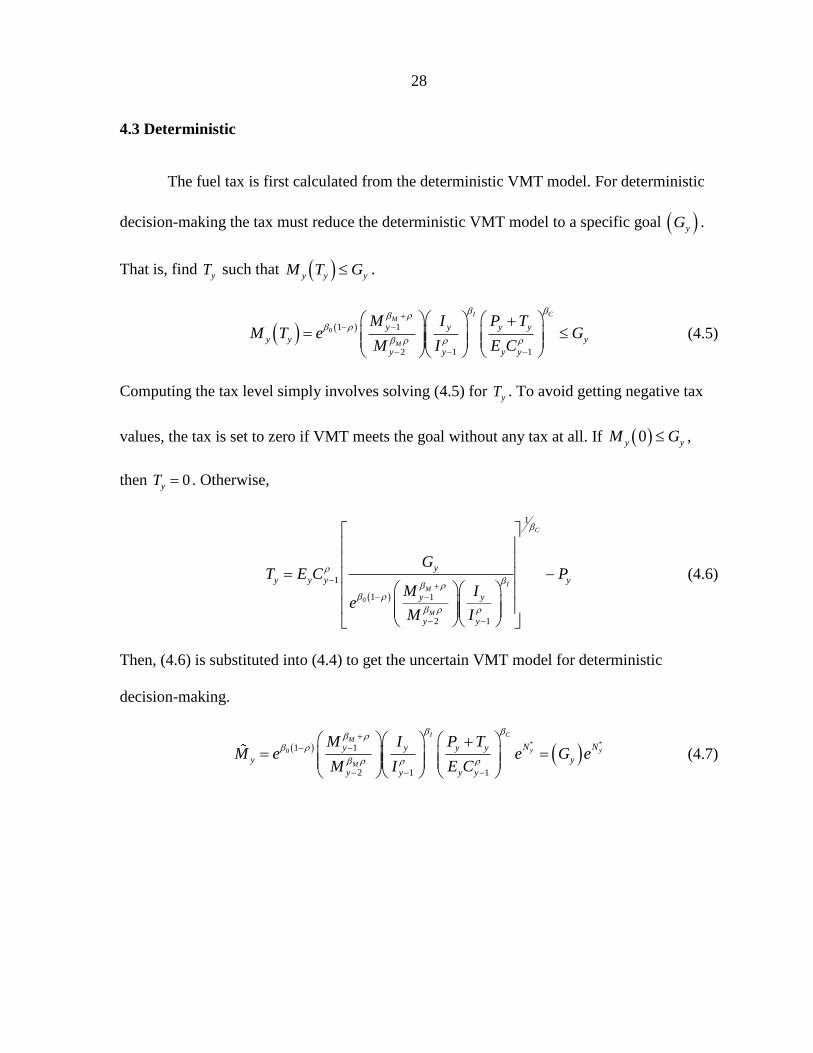
4.3 Deterministic

The fuel tax is first calculated from the deterministic VMT model. For deterministic

decision-making the tax must reduce the deterministic VMT model to a specific goal yG .

That is, find yT such that y y yM T G .

0 1 1

2 1 1

I CM

M

y y y y

y y y

y y y y

M I P TM T e G

M I E C

(4.5)

Computing the tax level simply involves solving (4.5) for yT . To avoid getting negative tax

values, the tax is set to zero if VMT meets the goal without any tax at all. If 0y yM G ,

then 0yT . Otherwise,

0

1

1

1 1

2 1

C

IM

M

y

y y y y

y y

y y

GT E C P

M Ie

M I

(4.6)

Then, (4.6) is substituted into (4.4) to get the uncertain VMT model for deterministic

decision-making.

* *0 1 1

2 1 1

I CM

y y

M

N Ny y y y

y y

y y y y

M I P TM e e G e

M I E C

(4.7)

29

4.4 Expected Value

Expected value decision-making consists of calculating the fuel tax necessary to force

the expected value of the uncertain VMT model to meet the goal. So, find yT such that

y y yE M T G

.

*

0 1 1

2 1 1

I CM

y

M

Ny y y y

y y y

y y y y

M I P TE M T e E e G

M I E C

(4.8)

If 0y yE M G , then 0yT . Otherwise,

*

0

1

1

1 1

2 1

C

IM

y

M

y

y y y y

Ny y

y y

GT E C P

M Ie E e

M I

(4.9)

Again, substituting this into (4.4) yields the probabilistic VMT model.

* *0

*

1 1

2 1 1

I CM

y y

My

N Ny y y y y

yN

y y y y

M I P T GM e e e

M I E C E e

(4.10)

4.5 Markovian

For Markovian decision-making the tax is found from the Markov chain yM . A

Markov chain is a discrete-time random process with the Markov property; the future state of

the process depends only on the present state, and not on the past. Let yM be the Markov

30

process defined below where yM is probabilistic, but considered a known variable in the

equation for yM . Then find yT such that y y yM T G .

0 1 1

2 1 1

I CM

M

y y y y

y y y

y y y y

M I P TM T e G

M I E C

(4.11)

If 0y yM G , then 0yT . Otherwise,

0

1

1

1 1

2 1

C

IM

M

y

y y y y

y y

y y

GT E C P

M Ie

M I

(4.12)

This time the tax is substituted into (4.3) to arrive at the uncertain VMT model.

0 1 1

2 1 1

I CM

y y

M

N Ny y y y

y y

y y y y

M I P TM e e G e

M I E C

(4.13)

4.6 Probabilistic

In probabilistic decision-making the policy maker is allowed to choose , the

certainty at which the target is met. Let 0.90 . Then a tax is found that gives a 90%

chance of meeting the goal. That is, find yT such that y y yP M T G .

31

*0

*

*

1 1

2 1 1

*

*

11 erf

2 2

I CM

y

M

y y

y

y

Ny y y y

y y y y

y y y y

y y y

T

N

y yN

y y

y

M I P TP M T G P e e G

M I E C

P N T

f n dn

F T

T

(4.14)

where

0 1 1

2 1 1

log log

I CM

M

y y y y

y y y

y y y y

M I P TT G e

M I E C

(4.15)

Then, (4.14) is solved for the tax level. If 0y yP M G , then 0yT . Otherwise,

0

*

* -1

1

1

1 1 * -1

2 1

11 erf

2 2

2 erf 2 1

exp 2 erf 2 1

C

IM

M

y y

y

y y y

y

y y y y

y y

y

y y

T

T

GT E C P

M Ie

M I

(4.16)

Substituting this tax into (4.4) gives the uncertain VMT model for probabilistic decision-

making.

32

*0

*

1 1

2 1 1

* -1exp 2 erf 2 1

I CM

y

M

y

Ny y y y

y

y y y y

Ny

y

M I P TM e e

M I E C

Ge

(4.17)

4.7 Results

Several plots are made to compare the results from each of the decision-making

techniques. In all of the figures in this section it appears as though there is no line for

deterministic decision-making, but this is not the case. In each figure the plots for

deterministic and expected value decision-making are so nearly identical that the expected

value plot covers up the deterministic plot. The deterministic and expected value equations

for VMT and the tax level are identical except for one term, the mean of the log normal

random variable *yN

e . Since *

1yNE e

, this term has almost no effect on the calculations.

Figure 6 shows an uncertain VMT projection from each of the methods. The

projection from probabilistic decision-making is below the other three projections, and

consistently below the target. In this particular figure the Markovian projection is similar to

the deterministic and expected value projections, and the three of them are mostly above the

target line. However, recall that these are uncertain VMT projections. New projections for

VMT will be plotted each time the MATLAB program is run. Because of this, the probability

density function (PDF) of VMT is plotted in Figure 7 to show the relative likelihood of VMT

violating the target in a given year.

33

Figure 6: Projections of uncertain VMT with a fuel tax.

Figure 7: PDFs of VMT in 2020.

Figure 7 shows projections from probabilistic decision-making are the most likely to

meet the target. The selection of in the probabilistic method can be graphically seen here,

because 90% of the probabilistic PDF is less than the target. The remaining three PDFs are

centered on the target, which shows their means are very close to the target. The Markovian

PDF is narrower than the deterministic and expected value PDFs. This suggests VMT

2010 2015 2020 2025 2030 20351.26

1.28

1.3

1.32

1.34

1.36

1.38

1.4x 10

4 How much will I drive each year?

Year

Mile

s

Target

Deterministic

Expected Value

Markovian

Probabilistic

11 11.5 12 12.5 13 13.5 14 14.5 150

0.5

1

1.5

2

2.5What is the PDF of VMT?

VMT ( thousand miles )

Target

Deterministic

Expected Value

Markovian

Probabilistic

34

projections from Markovian decision-making tend to be closer to the target. All of the PDFs

appear symmetric, indicating the mean and median of each method are very similar. Figure 8

gives a closer look at how the mean and median of each decision-making method compares

to the target. The mean and median from deterministic, expected value, and Markovian

decision-making fall right on the target line. In fact, the deterministic median, expected value

mean, and Markovian median are not plotted in Figure 8 because, by definition, they are

exactly equal to the target.

Figure 8: Mean and median VMT.

The purpose of this chapter is to show how the uncertain VMT equation can be used

to help policy makers decide on the best policy to reduce transportation GHG emissions.

Although projecting GHG emissions is beyond the scope of this research, emissions can be

represented by the amount of fuel consumed. Figure 9 and Figure 10 show projections for the

fuel consumed by each driver and by the entire US population.

2010 2015 2020 2025 2030 20351.26

1.28

1.3

1.32

1.34

1.36

1.38

1.4x 10

4 Will I meet the target?

Year

Mile

s

Target

Deterministic Mean VMT

Expected Value Median VMT

Markovian Mean VMT

Probabilistic Mean VMT

Probabilistic Median VMT

35

Figure 9: Projections of fuel consumption per licensed driver.

Figure 10: Projections of fuel consumption by all US drivers.

All four decision-making techniques project fuel consumption per licensed driver to

steadily decrease. It is especially rewarding to see that total US fuel consumption is also

expected to decline over time. Even though the US population, and therefore the number

vehicles being driven, will undoubtedly increase every year, the uncertain VMT model still

predicts total fuel consumption to decrease.

2010 2015 2020 2025 2030 2035440

460

480

500

520

540

560

580

600

620How much gasoline will I consume each year?

Year

Gallo

ns

Deterministic

Expected Value

Markovian

Probabilistic

2010 2015 2020 2025 2030 20351.38

1.4

1.42

1.44

1.46

1.48

1.5

1.52

1.54

1.56x 10

11 How much gasoline will everyone consume each year?

Year

Gallo

ns

Deterministic

Expected Value

Markovian

Probabilistic

36

Figure 10 provides evidence that a fuel tax would reduce GHG emissions. However,

this environmental benefit would come at a significant cost to drivers. Figure 11 gives the

fuel tax necessary for VMT to meet the specified target mileage. As expected, probabilistic

decision-making provides the highest projections of fuel tax. The total amount each driver

can expect to spend on the fuel tax ever year is plotted in Figure 12.

Figure 11: Projections of the fuel tax required to reduce VMT to the target.

Figure 12: Projections of the total fuel tax paid each year per licensed driver.

2010 2015 2020 2025 2030 20350

5

10

15How much tax will I pay for every gallon of gasoline?

Year

2000 d

olla

rs p

er

gallo

n

Deterministic

Expected Value

Markovian

Probabilistic

2010 2015 2020 2025 2030 20351000

2000

3000

4000

5000

6000

7000How much will I pay for taxes each year?

Year

2000 d

olla

rs

Deterministic

Expected Value

Markovian

Probabilistic

37

All four of the decision-making techniques discussed in this chapter achieve the

primary goal: a tax is calculated that effectively reduces VMT to a specified target, which

decreases the amount of transportation GHG emissions. Probabilistic decision-making is the

most drastic of the four methods. It projects the highest fuel tax, lowest VMT, and lowest

fuel consumption. However, it also allows policy makers to have the most control over the

VMT projections because any degree of certainty can be used. If the fuel tax seems too

extreme, then the target could be raised or the degree of certainty lowered to produce more

desirable forecasts. These methods could guide policy makers to better-informed policy

decisions, but they are only possible if some amount of uncertainty is incorporated into the

model.

38

CHAPTER 5: CONCLUSION

5.1 Summary

The National Energy Modeling System (NEMS) is a computational model that

forecasts the production, consumption, and prices of energy in the United States. Policy

makers rely heavily on NEMS forecasts to make informed energy policy decisions. These

forecasts depend significantly on a variety of economic assumptions, future oil prices,

consumer preferences and behaviors, new technologies yet to be developed, and numerous

other uncertain inputs. The uncertainties in NEMS need to be communicated to policy

makers in order for them to develop better-informed decisions regarding energy policy.

Part of the Transportation Module of NEMS projects the demand for personal travel

through its vehicle miles traveled (VMT) equation. In this research, uncertainty is added to

the VMT model as a prototype to demonstrate the importance and benefit of uncertainty in

NEMS. This starts with deriving the model and estimating its parameters. In order to find the

most appropriate estimation method, three different techniques are applied to the VMT

model: Cochrane-Orcutt, maximum likelihood, and Prais-Winsten. The maximum likelihood

and Prais-Winsten techniques are both preferred over Cochrane-Orcutt because they both

produce an estimate for , and the Cramér-Rao Lower Bound can be used to estimate the

standard errors of their parameters. Even though Prais-Winsten estimation attempts to

improve upon maximum likelihood estimation, its parameter estimates are found to fit the

historical data with less accuracy. Therefore, maximum likelihood is the best estimation

method for the VMT equation.

39

The maximum likelihood parameter estimates and their standard errors provide the

necessary statistics to add uncertainty to the parameters and the error term of the VMT

equation. A Monte Carlo simulation is performed to model the uncertain VMT equation and

demonstrate the range of possible VMT forecasts when these uncertainties are included. The

100 trajectories that are modeled suggest the NEMS deterministic forecast does not

adequately reflect all of the possible futures of VMT. Two more Monte Carlo simulations are

done to find the main source of uncertainty in the VMT model. This reveals that the error

term alone accounts for most of the uncertainty in the model. Simply adding a normal error

term to the model, while keeping the rest of the parameters and inputs deterministic, would

adequately represent the uncertainties present in the VMT model.

Transportation sources contribute nearly a third of the total US greenhouse gas

(GHG) emissions. Decreasing VMT is the most effective way to decrease GHG emissions,

and significant reductions in VMT can only be achieved by increasing the cost of driving

with a fuel tax. A target is set for VMT for each of the projected years, and four decision-

making techniques are used to calculate the fuel tax required to reduce VMT to this specified

goal. Deterministic, expected value, and Markovian decision-making all have a mean and

median very close or identical to the target. Their VMT projections meet the target about half

of the time. Probabilistic decision-making projects the highest fuel tax, lowest VMT, and

lowest fuel consumption. It also allows policy makers to decide the probability of the

projection meeting the target. All four decision-making techniques calculate a fuel tax that

reduces VMT to the target and decreases fuel consumption, thus reducing GHG emissions.

This demonstrates that an uncertain VMT equation can be used to help policy makers decide

on the best policy to reduce transportation GHG emissions.

40

5.2 Future Work

The Monte Carlo simulation used in Chapter 3 is an effective and practical method

for the purposes of this research. Only one uncertain equation is modeled, and only 100

random samples of the model are taken. If uncertainty was included in NEMS at a larger

scale, then Monte Carlo methods would no longer be practical. NEMS is a detailed and

complex model. Monte Carlo sampling from all of NEMS uncertain inputs would require far

too much computation time. Gentle (2002) describes faster sampling methods such as quasi-

random, importance, and Latin Hypercube sampling. However, even these methods require

too many evaluations of NEMS to be reasonable solutions. If uncertainty was included in

large portions of NEMS then stochastic collocation strategies must be applied to model this

uncertainty. Sparse grid collocation could model the uncertainty in NEMS with fast

convergence and without changing the current deterministic code (Ganapathysubramanian &

Zabaras, 2008).

41

APPENDIX A: VMT MODEL FOR PRAIS-WINSTEN ESTIMATION

The VMT model used in Prais-Winsten estimation is given below.

11 1

2

1 1

1

2,3,...,y y y y y

Nm x

m m x x N y Y

The Prais-Winsten model is unique in that it uses a different model for the first year of

known historical data. To derive this equation, start with the time series model for the first

year and repeatedly substitute in for y (2.3).

1 1 0 1

2

1 1 0 1

1 1 0 1

1 1

0

k

k

k

k

k

m x N

x N N

x N N

x N

(A.1)

The last term here is also a normal variable. So let 1 1

0

ˆ k

k

k

N N

where

2

1 2ˆ Normal 0,

1N

. The VMT model then becomes

2

1 1 1 1 2

2

2 2 1 2 2

2

1

ˆ ˆ Normal 0,1

Normal 0,

Normal 0,Y Y Y Y Y

m x N N

m x N N

m x N N

(A.2)

42

Notice that the normal error in the model for the first year has a different variance then the

rest of the normal errors. Prais-Winsten “corrects” this problem by making the assumption

2

1 1ˆ1 N N where 2

1 Normal 0,N . The final VMT model then becomes

2 2 2

1 1 1 1

2

2 2 1 2 2

2

1

1 1 Normal 0,

Normal 0,

Normal 0,Y Y Y Y Y

m x N N

m x N N

m x N N

(A.3)

43

APPENDIX B: VMT MODEL FOR DECISION-MAKING ANALYSIS

This appendix shows how the VMT model used in Chapter 2 is converted into the

VMT model used in Chapter 4. Only the probabilistic VMT model is derived here. The

deterministic model is derived exactly the same way, except there is no error term at the end

of the model. This may seem like a trivial review of algebra and logarithmic identities, but it

is important to see that the two models are the same, though they look very different.

1 0

1 2

1

1

1y y

M y y

I y y

C y y

y

m m

m m

i i

c c

N

(B.1)

1 0

1 2

1

1

log log 1

log log

log log

log log

y y

M y y

I y y

C y y

y

M M

M M

I I

C C

N

(B.2)

0

1 2

1

1

log 1

log log

log log

log log

y

M y M y

I y I y

C y C y

y

M

M M

I I

C C

N

(B.3)

44

0

1 2

1

1

log 1

log log

log log

log log

M M

I I

C C

y

y y

y y

y y

y

M

M M

I I

C C

N

(B.4)

1

0

2 1 1

log 1 log log logCM I

CM I

y y y

y y

y y y

M I CM N

M I C

(B.5)

1

0

2 1 1

log 1 logCM I

CM I

y y y

y y

y y y

M I CM N

M I C

(B.6)

0 1 1

2 1 1

CM I

y

CM I

Ny y y

y

y y y

M I CM e e

M I C

(B.7)

0 1 1

2 1 1

I CM

y

M

Ny y y

y

y y y

M I CM e e

M I C

(B.8)

0 1 1

2 1 1

I CM

y

M

Ny y y y

y

y y y y

M I P TM e e

M I E C

(B.9)

45

APPENDIX C: THE PROBABILISTIC VMT MODEL

Recall the deterministic (4.2) and probabilistic (4.3) VMT models used in Chapter 4

and derived in Appendix B.

0 1 1

2 1 1

I CM

M

y y y y

y

y y y y

M I P TM e

M I E C

0 1 1

2 1 1

I CM

y

M

Ny y y y

y

y y y y

M I P TM e e

M I E C

The three uncertain inputs of the probabilistic model need to be combined into one error term

for some of the analysis done in Chapter 4. To ease the notation, condense all of the

deterministic inputs of the probabilistic model into one term y .

1

2

M

y

M

Ny

y y

y

MM e

M

(C.1)

Now let 0M be the actual VMT from the year before the projection is made. Similarly, let

00M be the actual VMT from two years before the projection is made. Then the equation for

the first projected year is

101 1

00

M

M

NMM e

M

(C.2)

Notice that if the deterministic model was being used here its equation would be the same

except for the error term. So the probabilistic model can be written in terms of the

deterministic model.

46

101 1 1 1

00

M

M

NMM M M e

M

(C.3)

The equation for the second year is then calculated from (C.1), and (C.2) is substituted into

the model to get rid of the uncertainty in VMT.

2

2

1

2

2 2

2 1

12 2

0

01

00

2

0

02 1

00

M

M

M

M M

M M

M

M M

M M

M M

N

N

N

N N

MM e

M

Me

Me

M

Me

M

(C.4)

Again, this probabilistic equation is written in terms of its corresponding deterministic

equation.

2 2

2 102 2 1 2 2

00

M M

M M

M M

N NMM M M e

M

(C.5)

The same process is done to get an equation for the third year.

3

2 2

2 22 1

2

3

1

2 2

3 2 2 3

2 2

2

23 3

1

02 1

00

3

01

00

03 2 1

00

M

M

M M M

M M M M

M M

M M

MM

M

M M M

M M M

M M M

N

N N

N

N

MM e

M

Me

Me

Me

M

M

M

2 23 2 1

2

M M MN N Ne

(C.6)

47

2 2

3 2 1

3 3

M M MN N NM M e

(C.7)

At this point a pattern can be seen for the probabilistic VMT equation and its log normal

error. Let *

yN be the normal random variable such that

*1

*2

*3

*

1 1

2 2

3 3

y

N

N

N

N

y y

M M e

M M e

M M e

M M e

(C.8)

Substituting (4.2) into (C.8) yields the uncertain VMT model that is used in Chapter 4.

*0 1 1

2 1 1

I CM

y

M

Ny y y y

y

y y y y

M I P TM e e

M I E C

(C.9)

The new normal error *

yN is defined as follows.

1

2

2 2

3

3 2 2 3

4

1

1

1

M

M M

M M M

yy j j

y M

j

Q

Q

Q

Q

Q

(C.10)

*

1 1 1

*

2 1 2 2 1

*

3 1 3 2 2 3 1

*

4 1 4 2 3 3 2 4 1

*

1

1

y

y i y i

i

N Q N

N Q N Q N

N Q N Q N Q N

N Q N Q N Q N Q N

N Q N

(C.11)

48

REFERENCES

Baghelai, C., Moumen, F., Cohen, M., Kydes, A., & Harris, C. M. (1995a). Uncertainty in

the National Energy Modeling System I: Method Development. Journal of Energy

Engineering , 121 (3), 108-124.

Baghelai, C., Moumen, F., Cohen, M., Kydes, A., & Harris, C. M. (1995b). Uncertainty in

the National Energy Modeling System II: Analysis of Results. Journal of Energy

Engineering , 121 (3), 125-148.

Beach, C. M., & MacKinnon, J. G. (1978). A Maximum Likelihood Procedure for

Regression with Autocorrelated Errors. Econometrica , 46, 51-58.

Bureau of Economic Analysis. (2009, October). All NIPA Tables. Retrieved March 2011,

from http://www.bea.gov/national/nipaweb/SelectTable.asp?Selected=N

Cochrane, D., & Orcutt, G. H. (1949). Application of Least Spuares Regression to

Relationships Containing Auto-Correlated Error Terms. Journal of the American

Statistical Association , 44, 32-61.

DeCicco, J., & Mark, J. (1998). Meeting the energy and climate challenge for transportation

in the United States. Energy Policy , 26, 395-412.

Energy Information Administration. (2010a). Annual Energy Outlook 2010: With Projections

to 2035. Department of Energy, Washington D.C.

Energy Information Administration. (2010b, May). Annual Energy Outlook 2010. Retrieved

March 2011, from http://www.eia.gov/oiaf/archive/aeo10/index.html

Energy Information Administration. (2010c). Transportation Sector Module of the National

Energy Modeling System: Model Documentation 2010. Department of Energy,

Washington D.C.

Energy Information Administration. (2009). The National Energy Modeling System: An

Overview 2009. Department of Energy, Washington D.C.

Environmental Protection Agency. (2010, September). Transportation and Climate.

Retrieved March 2011, from http://www.epa.gov/otaq/climate/index.htm

Federal Highway Administration. (2010, December). Highway Statistics Publications.

Retrieved March 2011, from http://www.fhwa.dot.gov/policy/ohpi/hss/hsspubs.cfm

49

Fischer, C., Herrnstadt, E., & Morgenstern, R. (2009). Understanding errors in EIA

projections of energy demand. Resource and Energy Economics , 31, 198-209.

Gabriel, S. A., Kydes, A. S., & Whitman, P. (2001). The National Energy Modeling System:

A large-scale energy-economic equilibrium model. Operations Research , 49 (1), 14-

25.

Ganapathysubramanian, B., & Zabaras, N. (2008). A seamless approach towards stochastic

modeling: Sparse grid collocation and data driven input models. Finite Elements in

Analysis and Design , 44, 298-320.

Gentle, J. E. (2002). Elements of Computational Statistics. New York, NY: Springer Science

+ Business Media.

Greene, W. H. (2008). Econometric Analysis (6th ed.). Upper Saddle River, NJ: Pearson

Prentice Hall.

Greene, D. L., & Plotkin, S. E. (2001). Energy futures for the US transport sector. Energy

Policy , 29, 1255-1270.

Lady, G. M. (2010). Evaluating long term forecasts. Energy Economics , 32, 450-457.

Lempert, R. J., Popper, S. W., & Bankes, S. C. (2003). Shaping the next one hundred years:

new methods for quantitative, long-term policy analysis. Santa Monica, CA: RAND.

LeSage, J. P. (1999). Applied Econometrics using MATLAB. University of Toledo,

Department of Economics.

McCollum, D., & Yang, C. (2009). Achieving deep reductions in US transport greenhouse

gas emissions: Scenario analysis and policy implications. Energy Policy , 37, 5580-

5596.

Morrow, W. R., Gallagher, K. S., Collantes, G., & Lee, H. (2010). Analysis of policies to

reduce oil consumption and greenhouse gas emissions from the US transportation

sector. Enegy Policy , 38, 1305-1320.

O'Neill, B. C., & Desai, M. (2005). Accuracy of past projections of US energy consumption.

Energy Policy , 33, 979-993.

Prais, S. J., & Winsten, C. B. (1954). Trend Estimators and Serial Correlation. Cowles

Commission Discussion Paper: Statistics No. 383, Chicago.

Winebrake, J. J., & Sakva, D. (2006). An evaluation of errors in US energy forecasts: 1982-

2003. Energy Policy , 34, 3475-3483.