incorporation of inconel-718 material test data into

14th

International LS-DYNA Users Conference Session: Aerospace

June 12-14, 2016 1-1

Incorporation of Inconel-718 material test data into

material model input parameters for *MAT_224

Stefano Dolci1, Kelly Carney1, Leyu Wang1, Paul Du Bois2 and Cing-Dao Kan1

1Center for Collision Safety and Analysis, George Mason University, Fairfax, VA

2Consulting Engineer, Northville, MI

Abstract A research team from George Mason University, Ohio State University, NASA and FAA has

developed material data and analytical modeling that allows for precise input of material data into

LS-DYNA® using tabulation and the *MAT_224 material model. The input parameters of this model

are based on data from many experimental coupon tests including tension, compression, impact,

shear and biaxial stress states. The material model also includes temperature and strain rate effects.

This research effort involves the incorporation of the Inconel-718 material test data into the material

model. This requires the development and validation of a set of material constants for this particular

alloy, utilizing the tabulated input method of material model *MAT_224 in LS-DYNA with

consideration given to strain rate and temperature.

Alloy Inconel-718 is a precipitation hardenable nickel-based alloy designed to display exceptionally

high yield, tensile and creep-rupture properties at temperatures up to 1300°F. The sluggish age-

hardening response of alloy 718 permits annealing and welding without spontaneous hardening

during heating and cooling. This alloy has been used for jet engine and high-speed airframe parts

such as wheels, buckets, spacers, and high temperature bolts and fasteners.

*MAT_224 is an elastic-plastic material with arbitrary stress versus strain curve(s) and arbitrary

strain rate dependency, all of which can be defined by the user. Thermo-mechanical and

comprehensive plastic failure criterion can also be defined for the material. This requires a process

of test data reduction, stability checks, and smoothness checks to insure the model input can reliably

produce repeatable results. Desired curves are smooth and convex in the plastic region of the stress

strain curves.

Session: Aerospace 14th

International LS-DYNA Users Conference

1-2 June 12-14, 2016

Introduction Inconel718 is an important engineering material widely used in aerospace applications.

However, current constitutive models fall short in predicting the plastic and failure behavior of

this material under various strain rates. One reason for this may be the high dependency of the

properties of Inconel sheet on the manufacturing process and, hence, on the thickness of the

sheet. This research effort, therefore, involves the development and validation of a set of material

constants utilizing the tabulated input method of material model *MAT_224 in LS-DYNA with

consideration given to strain rate and temperature, specifically for a rolled ½-inch Inconel-718

sheet. *MAT_224 is an elastic-plastic material model with arbitrary stress versus strain curve(s)

and arbitrary strain rate dependency, all of which can be defined by the user. Thermo-mechanical

and comprehensive plastic failure criterion can also be defined for the material. [1]

The deformation portion of the Inconel-718 *MAT_224 inputs are based on the results of

uniaxial tensile testing conducted by Ohio State University [3][4][13] under plane stress

conditions at varying strain rates and temperatures. Material model development and validation

procedures are herein included as a reference for similar study.

Methodology Many factors contribute to the variations of Inconel-718 measured material properties, including,

but not limited to, the manufacturing and post-manufacturing processes, the test specimen

orientation in regards to plate grain direction, etc. To minimize some of these discrepancies, the

material studied here is Inconel-718 ½-inch plate manufactured by a sole company.

The ½-inch rolled plate metal Inconel-718 material is modeled using *MAT_224 in LS-DYNA.

This is an isotropic elasto-thermo-visco-plastic constitutive relationship which states that stress is

dependent on strain, strain rate and temperature:

),,( Tijijijij

Equation 1

Where ij is stress, ij is strain, ɛ̇ij is the strain rate, and T is the temperature. In the elastic

region, the Jaumann rate of the stress tensor,

ij, is obtained as a linear function of elastic strain

rates; this is a generalization of hypo-elasticity:

p

ijijij

p

kkkkij 2

Equation 2

Here ɛ ̇ p

ij are the components of the plastic strain rate tensor and and µ are Lamé constants.

Young's modulus, E, and Poisson's ratio, , may be converted by:

)23(E

Equation 3

)(2

Equation 4

14th


June 12-14, 2016 1-3

The material response in the plastic region is determined by a von Mises-type yield surface in a

six-dimension stress space that can expand and/or contract due to strain hardening, rate effects

and thermal softening:

),,(),,( TT p

eff

p

effy

p

ij

p

ijyijvm

Equation 5

Where vm is the von Mises stress, ɛ p

eff is the equivalent plastic strain and ɛ ̇ p

eff is the equivalent

plastic strain rate. As the material is assumed isotropic, the dependency of the yield surface upon

plastic strain and plastic strain rate can be expressed purely as a function of the second invariant

of each tensor. Note that states on the yield surface are plastic, whereas states below the yield

surface are elastic. Mathematically this is expressed as follows:

0),,(

0

0),,(

T

T

p

eff

p

effyijvm

p

eff

p

eff

p

eff

p

effyijvm

Equation 6

The plastic strain rates are determined by associated flow leading to the well-known plastic

incompressibility condition typical of metals:

03

1

k

p

kk

ij

vmp

eff

p

ij

Equation 7

Common Elastic-Plastic Modeling Revisited A review of common plastic material modeling procedures will demonstrate the limitations and

error that can be introduced in the process. What follows is a detailed review, including typical

assumptions, of the typical elastic-plastic material modeling procedure.

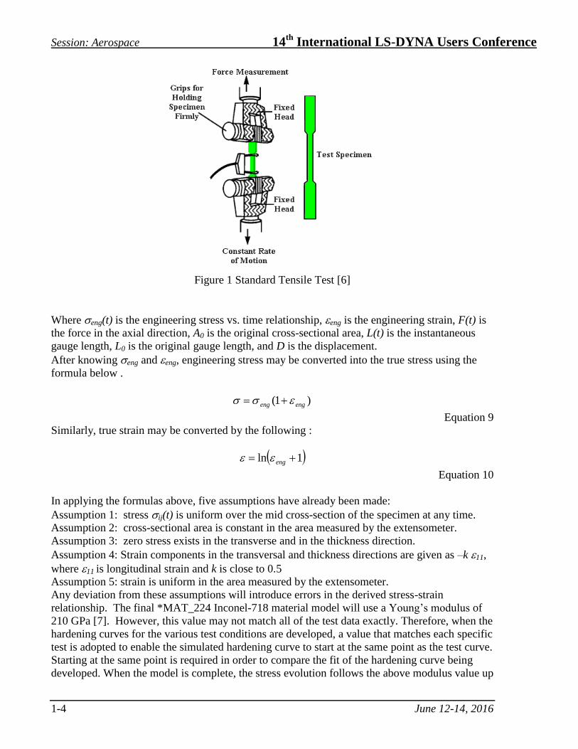
The material modeling begins with a standardized tensile test. A dog-bone specimen under a

constant grip speed is pulled in a test machine (Figure 1). Two measurements are recorded, the

force vs. time relationship, F (t), is measured with the tensile machine, and the displacement vs.

time relationship, D (t), is measured by a gauge or an extensometer fixed to the specimen. The

force vs. displacement curve is then generated by cross-plotting these two curves.

After acquiring the force vs. displacement curve, simple formulas are used to calculate

engineering stress and engineering strain.

00

0

0

L

tD

L

LtLt

A

tFt

eng

eng

Equation 8



1-4 June 12-14, 2016

Figure 1 Standard Tensile Test [6]

Where eng(t) is the engineering stress vs. time relationship, eng is the engineering strain, F(t) is

the force in the axial direction, A0 is the original cross-sectional area, L(t) is the instantaneous

gauge length, L0 is the original gauge length, and D is the displacement.

After knowing eng and eng, engineering stress may be converted into the true stress using the

formula below .

)1( engeng

Equation 9

Similarly, true strain may be converted by the following :

1ln eng

Equation 10

In applying the formulas above, five assumptions have already been made:

Assumption 1: stress ij(t) is uniform over the mid cross-section of the specimen at any time.

Assumption 2: cross-sectional area is constant in the area measured by the extensometer.

Assumption 3: zero stress exists in the transverse and in the thickness direction.

Assumption 4: Strain components in the transversal and thickness directions are given as –k 11,

where 11 is longitudinal strain and k is close to 0.5

Assumption 5: strain is uniform in the area measured by the extensometer.

Any deviation from these assumptions will introduce errors in the derived stress-strain

relationship. The final *MAT_224 Inconel-718 material model will use a Young’s modulus of

210 GPa [7]. However, this value may not match all of the test data exactly. Therefore, when the

hardening curves for the various test conditions are developed, a value that matches each specific

test is adopted to enable the simulated hardening curve to start at the same point as the test curve.

Starting at the same point is required in order to compare the fit of the hardening curve being

developed. When the model is complete, the stress evolution follows the above modulus value up

14th


June 12-14, 2016 1-5

to the proportional limit departure point for the different hardening curves, depending upon stress

state, rate and temperature.

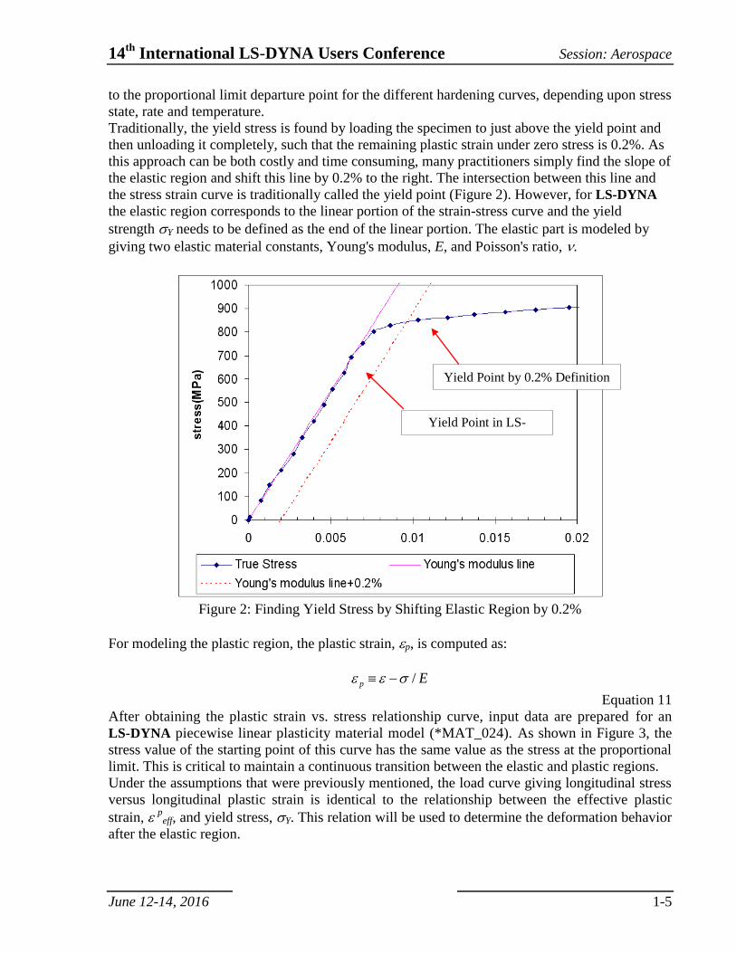
Traditionally, the yield stress is found by loading the specimen to just above the yield point and

then unloading it completely, such that the remaining plastic strain under zero stress is 0.2%. As

this approach can be both costly and time consuming, many practitioners simply find the slope of

the elastic region and shift this line by 0.2% to the right. The intersection between this line and

the stress strain curve is traditionally called the yield point (Figure 2). However, for LS-DYNA

the elastic region corresponds to the linear portion of the strain-stress curve and the yield

strength Y needs to be defined as the end of the linear portion. The elastic part is modeled by

giving two elastic material constants, Young's modulus, E, and Poisson's ratio, .

Figure 2: Finding Yield Stress by Shifting Elastic Region by 0.2%

For modeling the plastic region, the plastic strain, p, is computed as:

Ep /

Equation 11

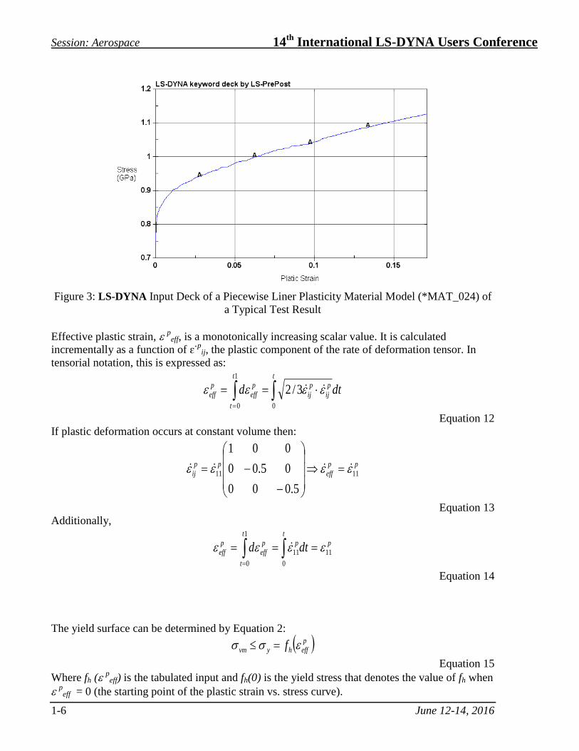
After obtaining the plastic strain vs. stress relationship curve, input data are prepared for an

LS-DYNA piecewise linear plasticity material model (*MAT_024). As shown in Figure 3, the

stress value of the starting point of this curve has the same value as the stress at the proportional

limit. This is critical to maintain a continuous transition between the elastic and plastic regions.

Under the assumptions that were previously mentioned, the load curve giving longitudinal stress

versus longitudinal plastic strain is identical to the relationship between the effective plastic

strain, peff, and yield stress, Y. This relation will be used to determine the deformation behavior

after the elastic region.

Yield Point in LS-

DYNA

Yield Point by 0.2% Definition



1-6 June 12-14, 2016

Figure 3: LS-DYNA Input Deck of a Piecewise Liner Plasticity Material Model (*MAT_024) of

a Typical Test Result

Effective plastic strain, peff, is a monotonically increasing scalar value. It is calculated

incrementally as a function of ɛ̇ p

ij, the plastic component of the rate of deformation tensor. In

tensorial notation, this is expressed as:

dtd

t

p

ij

p

ij

t

t

p

eff

p

eff 0

1

0

3/2

Equation 12

If plastic deformation occurs at constant volume then:

pp

eff

pp

ij 1111

5.000

05.00

001

Equation 13

Additionally,

p

t

p

t

t

p

eff

p

eff dtd 11

0

11

1

0

Equation 14

The yield surface can be determined by Equation 2:

p

effhyvm f

Equation 15

Where fh (p

eff) is the tabulated input and fh(0) is the yield stress that denotes the value of fh when

peff = 0 (the starting point of the plastic strain vs. stress curve).

14th


June 12-14, 2016 1-7

The effective stress according to von Mises, vm, is defined as follows:

222222 666)()()(2

1zxyzxyxzzyyxvm

Equation 16

It can be observed that it is identical to the longitudinal stress under conditions of uniaxial

tension:

0

000

000

001

111111

vmij

Equation 17

Violations of Common Assumptions The common method for modeling elastic-plastic materials presented in the previous section is

invalid after the necking point because at least three out of five assumptions are violated.

Assumption 1 is still considered valid because the stress ij(t) varies little over the cross-

sectional area at any time.

Assumption 4 is still valid because the material remains isotropic and plastically incompressible

after onset of the plastic instability.

Assumption 2 is invalid, as the cross-sectional area is much smaller in the localized region after

necking and therefore not a constant in the region spanned by an extensometer.

Assumption 3 is invalid, as transversal stresses will develop after the onset of necking and

additional stresses in the thickness direction will develop after the onset of local necking.

Consequently, after necking the specimen is no longer in a uniaxial stress condition.

Before necking, under uniaxial stress conditions, the only non-zero stress component is the axial

stress, l:

lvm

l

000

000

00

Equation 18

After necking, a transverse stress, t, appears because the material will resist shrinking in the

transverse direction:

lvmt

l

000

00

00

Equation 19

As the local necking develops we see additional stresses in the thickness direction, tt:

lvm

tt

t

l

00

00

00

Equation 20

An accurate measurement of l can be obtained by applying the instantaneous necking cross-

sectional area (measured by digital imaging) in the stress calculation. It is, however, not possible



1-8 June 12-14, 2016

to measure the transverse stress, t, nor the thickness stress, tt. Therefore, vm is generally

unknown after necking. If the uniaxial stress assumption is still applied (assume vm ≈ t after

necking) and this false von Mises stress vs. effective plastic strain relationship is used to define

the behavior of material, then the simulation result will deviate from the real test.

Assumption 5 is invalid because the strain is not uniform within the measuring distance of the

extensometer. After the onset of necking, the neck will have a higher strain than the rest of the

part. An accurate measurement of strain the region of necking can be obtained via a digital image

correlation (DIC).

Stress Strain Relationship after Necking In order to create an accurate material model and simulate the tensile test in LS-DYNA, the

method used is as follows: Start by estimating several post-necking plastic stress-strain curves as

input by extrapolating the curve before necking. Then compare the simulation force vs.

displacement curve with test results and pick the input curve that gives the closest match. Note

that the complete specimen geometry must be precisely modeled by measuring the actual

specimen, rather than using the design values on the blueprint. Also note that at this stage in the

process, the strain rate effect is not considered in the simulation. Next, input a single stress-strain

curve associated with a particular strain rate, thereby making the material model strain rate

independent. In other words, at this point in the modeling process, the material model will

behave the same no matter the loading speed, as long as inertia effects are sufficiently small.

Because of this strain rate independence, the simulation can be performed with an arbitrary

(higher) loading speed instead of the actual loading speed that was used in the test, allowing for a

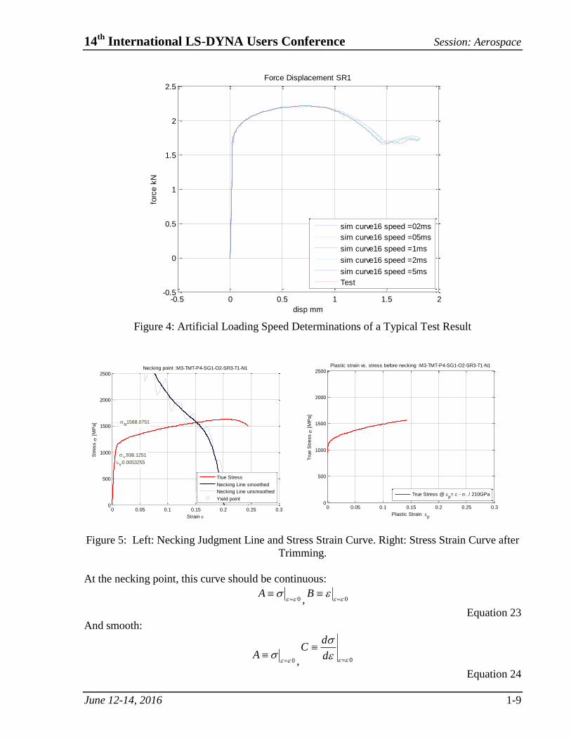
much shorter simulation time. To safely implement the method, one must run several simulations

to determine a good artificial loading speed in the simulation (Figure 4).

The rate-independent material model will have a dynamic effect if loaded at a very high speed

due to the inertia effects. Therefore, start with a high loading speed of 10 m/s and gradually

reduce it to the point where further reduction no longer changes the results. Use that final speed

for loading the simulation; in this case, it is 1 m/s.

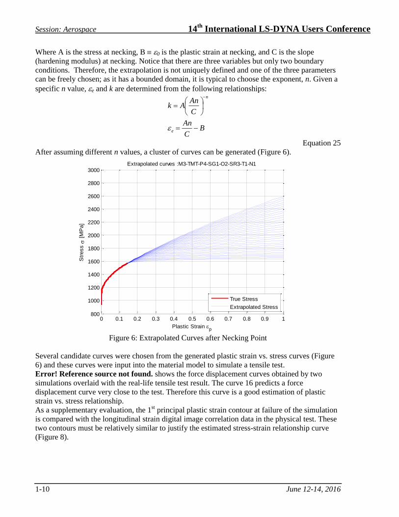
The necking point is identified by making the assumption that necking occurs at maximum load .

The necking point is given by the intersection between the true strain versus true stress curve and

its own derivative. So necking occurs where the true stress is equal to the tangent modulus:

d

d

)(

Equation 21

The hardening curves are extrapolated after necking using the following formula:

npek

Equation 22

Where k, e, and n are fitting parameters and the exponent n is expected to vary between 0 and 1

as the hardening curve is expected to be monotonically increasing and to have a monotonically

decreasing tangent.

After the necking point is determined, only the part of the strain-stress curve before necking is

used for further processing (Figure 5).

14th


June 12-14, 2016 1-9

-0.5 0 0.5 1 1.5 2-0.5

0

0.5

1

1.5

2

2.5Force Displacement SR1

disp mm

forc

e k

N

sim curve16 speed =02ms





Test

Figure 4: Artificial Loading Speed Determinations of a Typical Test Result

0 0.05 0.1 0.15 0.2 0.25 0.30

500

1000

1500

2000

2500Necking point :M3-TMT-P4-SG1-O2-SR3-T1-N1

Strain

Str

ess

[M

Pa]

N1568.0751

N0.15187

Y

938.1251

Y

0.0053255

True Stress

Necking Line smoothed

Necking Line unsmoothed

Yield point

0 0.05 0.1 0.15 0.2 0.25 0.30

500

1000

1500

2000

2500Plastic strain vs. stress before necking :M3-TMT-P4-SG1-O2-SR3-T1-N1

Plastic Strain p

Tru

e S

tress

[M

Pa]

True Stress @ p= - . / 210GPa

Figure 5: Left: Necking Judgment Line and Stress Strain Curve. Right: Stress Strain Curve after

Trimming.

At the necking point, this curve should be continuous:

0

A

, 0

B

Equation 23

And smooth:

0

A

, 0

d

dC

Equation 24



1-10 June 12-14, 2016

Where A is the stress at necking, B 0 is the plastic strain at necking, and C is the slope

(hardening modulus) at necking. Notice that there are three variables but only two boundary

conditions. Therefore, the extrapolation is not uniquely defined and one of the three parameters

can be freely chosen; as it has a bounded domain, it is typical to choose the exponent, n. Given a

specific n value, e and k are determined from the following relationships:

BC

An

C

AnAk

e

n

Equation 25

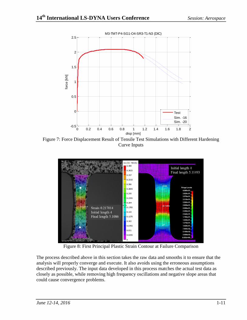
After assuming different n values, a cluster of curves can be generated (Figure 6).

0 0.1 0.2 0.3 0.4 0.5 0.6 0.7 0.8 0.9 1800

1000

1200

1400

1600

1800

2000

2200

2400

2600

2800

3000Extrapolated curves :M3-TMT-P4-SG1-O2-SR3-T1-N1

Plastic Strain p

Str

ess

[M

Pa]

True Stress

Extrapolated Stress

Figure 6: Extrapolated Curves after Necking Point

Several candidate curves were chosen from the generated plastic strain vs. stress curves (Figure

6) and these curves were input into the material model to simulate a tensile test.

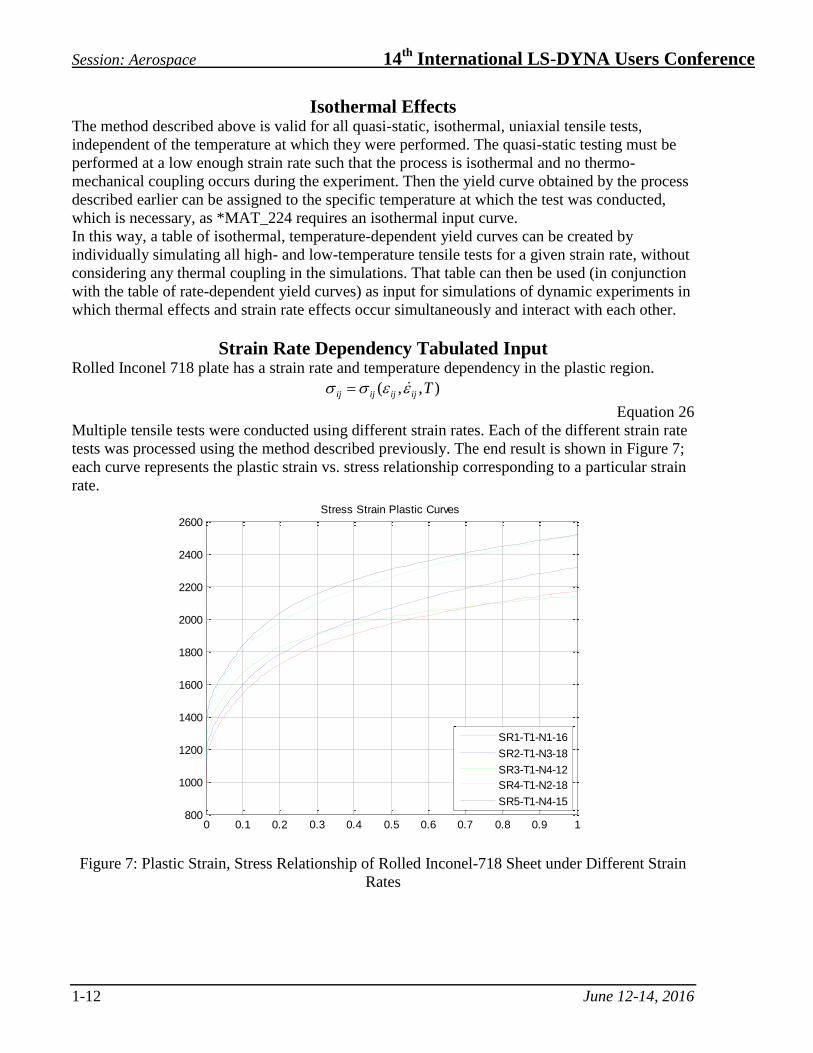
Error! Reference source not found. shows the force displacement curves obtained by two

simulations overlaid with the real-life tensile test result. The curve 16 predicts a force

displacement curve very close to the test. Therefore this curve is a good estimation of plastic

strain vs. stress relationship.

As a supplementary evaluation, the 1st principal plastic strain contour at failure of the simulation

is compared with the longitudinal strain digital image correlation data in the physical test. These

two contours must be relatively similar to justify the estimated stress-strain relationship curve

(Figure 8).

14th


June 12-14, 2016 1-11

0 0.2 0.4 0.6 0.8 1 1.2 1.4 1.6 1.8 2-0.5

0

0.5

1

1.5

2

2.5M3-TMT-P4-SG1-O4-SR3-T1-N3 (DIC)

disp [mm]

forc

e [

kN

]

Test

Sim. -16

Sim. -20

Figure 7: Force Displacement Result of Tensile Test Simulations with Different Hardening

Curve Inputs

Figure 8: First Principal Plastic Strain Contour at Failure Comparison

The process described above in this section takes the raw data and smooths it to ensure that the

analysis will properly converge and execute. It also avoids using the erroneous assumptions

described previously. The input data developed in this process matches the actual test data as

closely as possible, while removing high frequency oscillations and negative slope areas that

could cause convergence problems.



1-12 June 12-14, 2016

Isothermal Effects The method described above is valid for all quasi-static, isothermal, uniaxial tensile tests,

independent of the temperature at which they were performed. The quasi-static testing must be

performed at a low enough strain rate such that the process is isothermal and no thermo-

mechanical coupling occurs during the experiment. Then the yield curve obtained by the process

described earlier can be assigned to the specific temperature at which the test was conducted,

which is necessary, as *MAT_224 requires an isothermal input curve.

In this way, a table of isothermal, temperature-dependent yield curves can be created by

individually simulating all high- and low-temperature tensile tests for a given strain rate, without

considering any thermal coupling in the simulations. That table can then be used (in conjunction

with the table of rate-dependent yield curves) as input for simulations of dynamic experiments in

which thermal effects and strain rate effects occur simultaneously and interact with each other.

Strain Rate Dependency Tabulated Input Rolled Inconel 718 plate has a strain rate and temperature dependency in the plastic region.

),,( Tijijijij

Equation 26

Multiple tensile tests were conducted using different strain rates. Each of the different strain rate

tests was processed using the method described previously. The end result is shown in Figure 7;

each curve represents the plastic strain vs. stress relationship corresponding to a particular strain

rate.

0 0.1 0.2 0.3 0.4 0.5 0.6 0.7 0.8 0.9 1800

1000

1200

1400

1600

1800

2000

2200

2400

2600Stress Strain Plastic Curves

SR1-T1-N1-16

SR2-T1-N3-18

SR3-T1-N4-12

SR4-T1-N2-18

SR5-T1-N4-15

Figure 7: Plastic Strain, Stress Relationship of Rolled Inconel-718 Sheet under Different Strain

Rates

14th


June 12-14, 2016 1-13

Strain Rate Is Not a Constant Initially, the strain rate is assumed to be either the nominal strain rate of the test, or the grip

speed divided by the initial length of the sample covered by the extensometer. However, this

assumption is incorrect, and there are two reasons. First, it is easy to show that:

dt

dl

tlt

dt

d

)(

1)(

Equation 27

Consequently, the strain rate is not constant under constant grip loading speed. Although the

strain rate is uniform over the sample until necking occurs, it varies (decreases) with time if the

grip speed is constant.

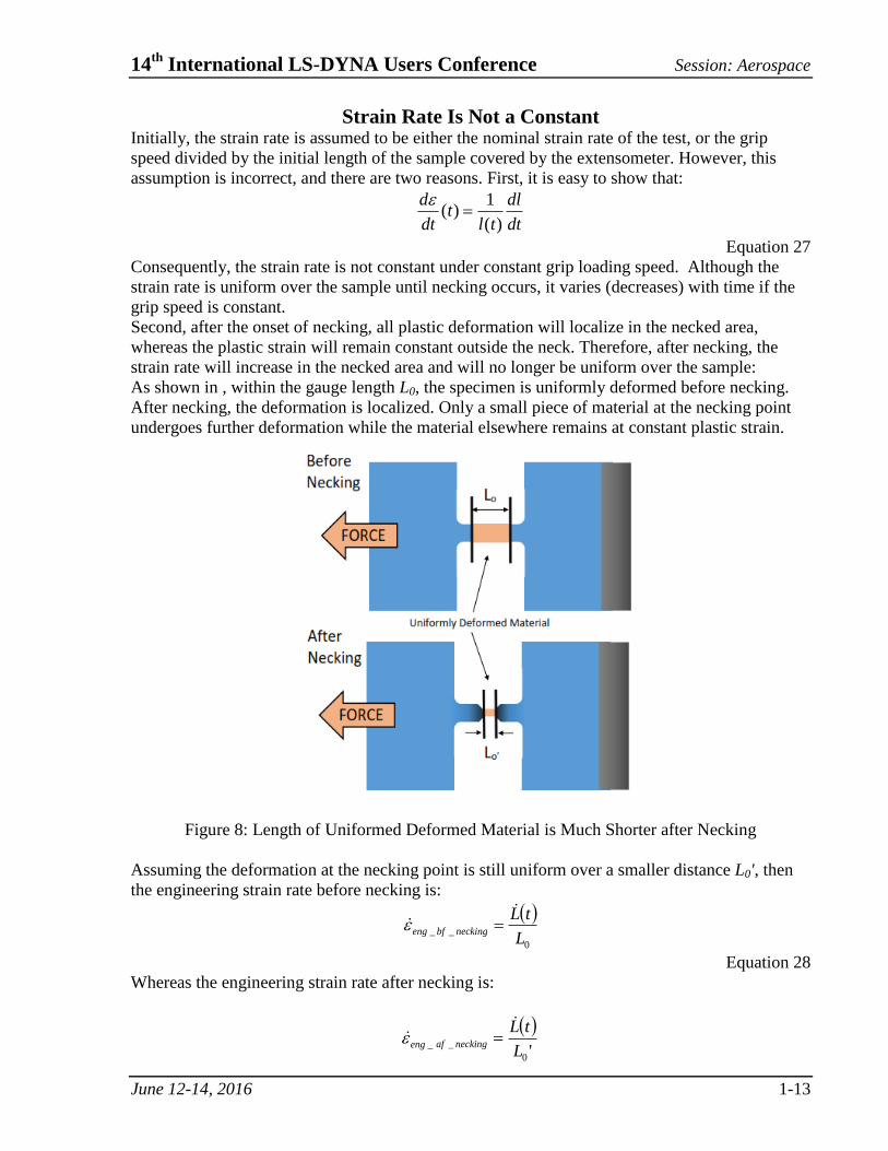
Second, after the onset of necking, all plastic deformation will localize in the necked area,

whereas the plastic strain will remain constant outside the neck. Therefore, after necking, the

strain rate will increase in the necked area and will no longer be uniform over the sample:

As shown in , within the gauge length L0, the specimen is uniformly deformed before necking.

After necking, the deformation is localized. Only a small piece of material at the necking point

undergoes further deformation while the material elsewhere remains at constant plastic strain.

Figure 8: Length of Uniformed Deformed Material is Much Shorter after Necking

Assuming the deformation at the necking point is still uniform over a smaller distance L0', then

the engineering strain rate before necking is:

0

__L

tLneckingbfeng

Equation 28

Whereas the engineering strain rate after necking is:

'0

__L

tLneckingafeng

0

__L

tLneckingbfeng



1-14 June 12-14, 2016

Equation 29

And consequently it is shown that the engineering strain rate will increase considerably in the

necked area:

neckingbfengneckingafeng

LL

____

00 '

Equation 30

The same tendency is true for the true strain rate, although somewhat more difficult to show.

Other variations in the testing procedure (e.g. non-constant grip speed, non-fixed boundary

conditions, etc.) may also influence the strain rate value and cause the nominal strain rate to

deviate from the physical value. Therefore, the measured displacement time history from the test

must be input into the numerical model to accurately simulate the strain rates that occurred in

each test.

High Strain Rate Sensitivity As described in the previous section, the strain rate in a test with localization is not a constant.

Localization is especially early and extreme in the higher strain rate Inconel-718 tests. The strain

rate in the region of localization may reach values significantly above the nominal strain rate for

the specimen. As a result, tension test data must be supplemented with synthetic curves

generated using rate sensitivity trends from tension and compression tests. The compression tests

reached much higher strain rates than the tension test but, due to friction and boundary

conditions, complete stress-strain curves are difficult to derive from compression tests.

Therefore, synthetic curves are created using a combination of information from the compression

and tension tests. These synthetic curves are combined with the stress-strain curves derived

directly from the tension tests. The tests referenced below were performed by Ohio State

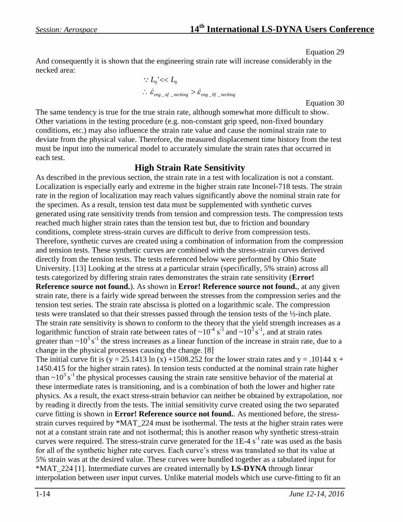
University. [13] Looking at the stress at a particular strain (specifically, 5% strain) across all

tests categorized by differing strain rates demonstrates the strain rate sensitivity (Error!

Reference source not found.). As shown in Error! Reference source not found., at any given

strain rate, there is a fairly wide spread between the stresses from the compression series and the

tension test series. The strain rate abscissa is plotted on a logarithmic scale. The compression

tests were translated so that their stresses passed through the tension tests of the ½-inch plate.

The strain rate sensitivity is shown to conform to the theory that the yield strength increases as a

logarithmic function of strain rate between rates of ~10-4

s-1

and ~103 s

-1, and at strain rates

greater than ~103

s-1

the stress increases as a linear function of the increase in strain rate, due to a

change in the physical processes causing the change. [8]

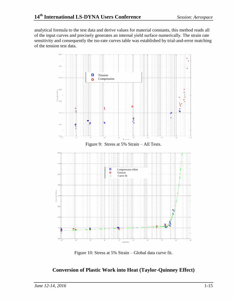
The initial curve fit is (y = 25.1413 ln (x) +1508.252 for the lower strain rates and y = .10144 x +

1450.415 for the higher strain rates). In tension tests conducted at the nominal strain rate higher

than ~103

s-1

the physical processes causing the strain rate sensitive behavior of the material at

these intermediate rates is transitioning, and is a combination of both the lower and higher rate

physics. As a result, the exact stress-strain behavior can neither be obtained by extrapolation, nor

by reading it directly from the tests. The initial sensitivity curve created using the two separated

curve fitting is shown in Error! Reference source not found.. As mentioned before, the stress-

strain curves required by *MAT_224 must be isothermal. The tests at the higher strain rates were

not at a constant strain rate and not isothermal; this is another reason why synthetic stress-strain

curves were required. The stress-strain curve generated for the 1E-4 s-1

rate was used as the basis

for all of the synthetic higher rate curves. Each curve’s stress was translated so that its value at

5% strain was at the desired value. These curves were bundled together as a tabulated input for

*MAT_224 [1]. Intermediate curves are created internally by LS-DYNA through linear

interpolation between user input curves. Unlike material models which use curve-fitting to fit an

14th


June 12-14, 2016 1-15

analytical formula to the test data and derive values for material constants, this method reads all

of the input curves and precisely generates an internal yield surface numerically. The strain rate

sensitivity and consequently the iso-rate curves table was established by trial-and-error matching

of the tension test data.

Figure 9: Stress at 5% Strain – All Tests.

Figure 10: Stress at 5% Strain – Global data curve fit.

Conversion of Plastic Work into Heat (Taylor-Quinney Effect)

Tension

Compression

Compression offset

Tension

Curve fit



1-16 June 12-14, 2016

In the higher rate tests within the localized region of necking, there is not sufficient time for

conduction to carry away the heat generated by the plastic deformation, and so the process

becomes adiabatic. This adiabatic process causes a significant increase in the temperature of the

specimen locally and governs the behavior at larger strains. As a result, the simulation of the

tension tests is sensitive to the amount of energy generated by the plastic work, which is

converted into thermal energy.

The percentage of plastic work that is converted into thermal energy is defined by the Taylor-

Quinney coefficient, typically signified as β. Research by Ravichandran [9] and Rosakis Error!

Reference source not found. yielded values for the Taylor-Quinney coefficient for α-titanium

which were not constant, but were a function of both strain rate and, to a lesser extent, plastic

strain. Additionally, [9] and Error! Reference source not found. also present variable values of

β’s for Al2024, which are a strong function of plastic strain. The capability to input a variable β

in *MAT_224 is available, but no published data for the Taylor-Quinney coefficient for Inconel-

718 is available. Independent measurements of temperature rise in high rate deformation are

planned by OSU, but are not yet available. Therefore, a constant β value of .8, which best

matched the stress-strain test behavior exhibited in the tension tests, was determined through

trial-and-error.

With this information, a fully coupled thermal solution using *MAT_224 in LS-DYNA could be

performed. This simulates the conduction of thermal energy away from highly strained elements.

Without including conduction, temperatures will rise more in the simulations than in tests,

leading to non-physical analytical results. This non-physical result will be very small in high

rate, short duration simulations, and can be safely ignored. In simulations where both high rate

and low rate loading takes place simultaneously and significant strains are introduced into

elements at a lower rate (i.e. longer duration simulation, such as full engine blade loss) as well as

at high rates, including conduction may be required for accurate analysis.

Material Model Creation by Simulation of Mechanical Property Tests

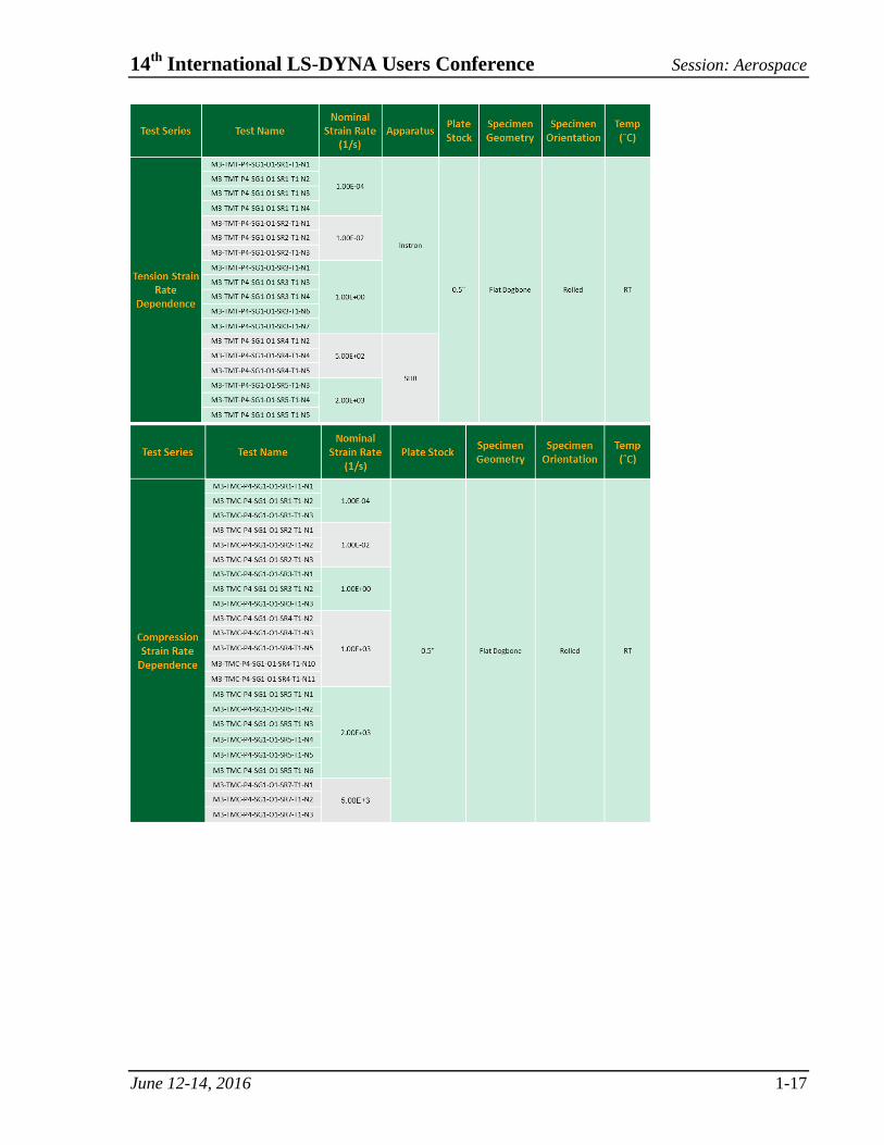
Test Data The test data includes time, force and displacement information. Every test comes with a CAD

image showing the exact specimen dimensions from measurement. A DIC imagine taken at the

time of failure (the last data point of the test data) is also included. The tests in Table 1 are

provided by Ohio State University [13].

14th


June 12-14, 2016 1-17



1-18 June 12-14, 2016

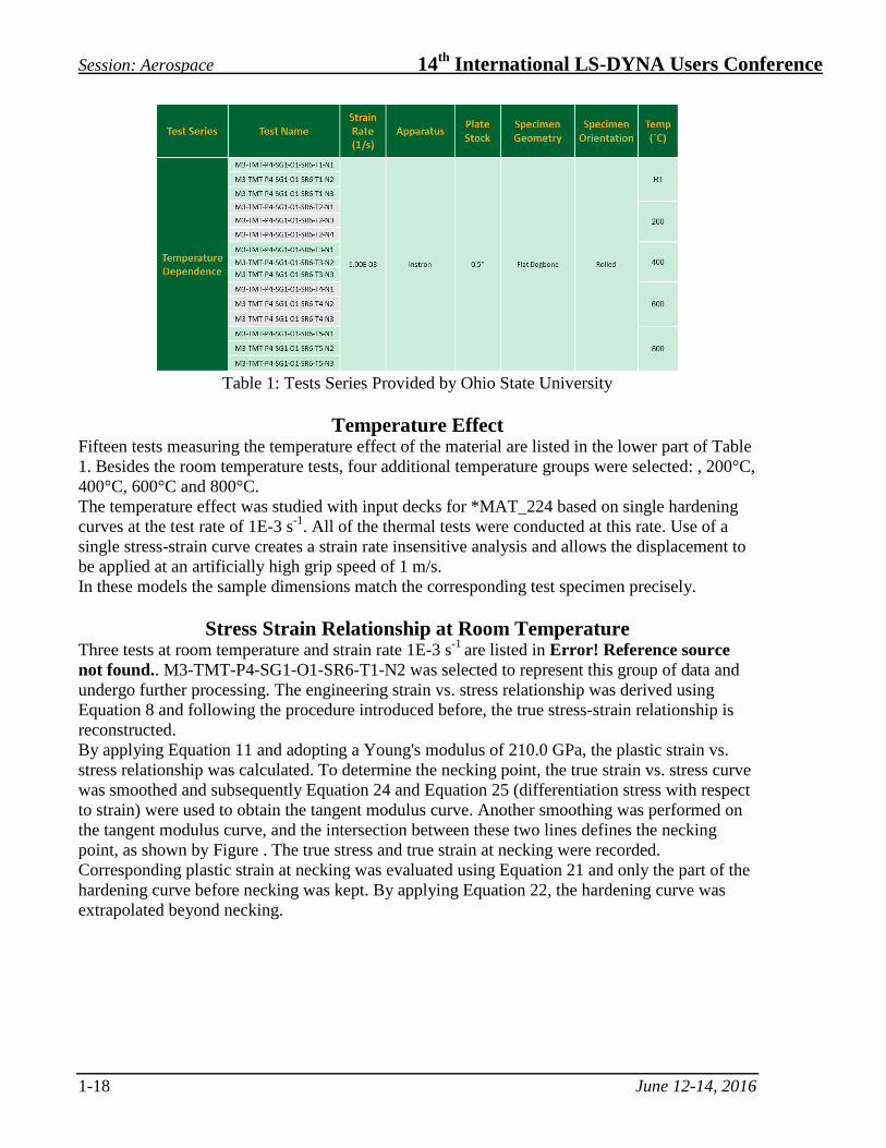
Table 1: Tests Series Provided by Ohio State University

Temperature Effect Fifteen tests measuring the temperature effect of the material are listed in the lower part of Table

1. Besides the room temperature tests, four additional temperature groups were selected: , 200°C,

400°C, 600°C and 800°C.

The temperature effect was studied with input decks for *MAT_224 based on single hardening

curves at the test rate of 1E-3 s-1

. All of the thermal tests were conducted at this rate. Use of a

single stress-strain curve creates a strain rate insensitive analysis and allows the displacement to

be applied at an artificially high grip speed of 1 m/s.

In these models the sample dimensions match the corresponding test specimen precisely.

Stress Strain Relationship at Room Temperature Three tests at room temperature and strain rate 1E-3 s

-1 are listed in Error! Reference source

not found.. M3-TMT-P4-SG1-O1-SR6-T1-N2 was selected to represent this group of data and

undergo further processing. The engineering strain vs. stress relationship was derived using

Equation 8 and following the procedure introduced before, the true stress-strain relationship is

reconstructed.

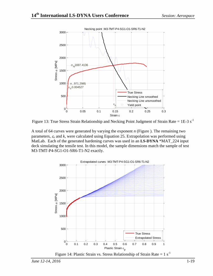
By applying Equation 11 and adopting a Young's modulus of 210.0 GPa, the plastic strain vs.

stress relationship was calculated. To determine the necking point, the true strain vs. stress curve

was smoothed and subsequently Equation 24 and Equation 25 (differentiation stress with respect

to strain) were used to obtain the tangent modulus curve. Another smoothing was performed on

the tangent modulus curve, and the intersection between these two lines defines the necking

point, as shown by Figure . The true stress and true strain at necking were recorded.

Corresponding plastic strain at necking was evaluated using Equation 21 and only the part of the

hardening curve before necking was kept. By applying Equation 22, the hardening curve was

extrapolated beyond necking.

14th


June 12-14, 2016 1-19

0 0.05 0.1 0.15 0.2 0.25 0.30

500

1000

1500

2000

2500

3000Necking point :M3-TMT-P4-SG1-O1-SR6-T1-N2

Strain

Str

ess

[M

Pa]

N1697.4136

N0.14454

Y

971.2985

Y

0.004527

True Stress

Necking Line smoothed

Necking Line unsmoothed

Yield point

Figure 13: True Stress Strain Relationship and Necking Point Judgment of Strain Rate = 1E-3 s

-1

A total of 64 curves were generated by varying the exponent n (Figure ). The remaining two

parameters, e and k, were calculated using Equation 25. Extrapolation was performed using

MatLab. Each of the generated hardening curves was used in an LS-DYNA *MAT_224 input

deck simulating the tensile test. In this model, the sample dimensions match the sample of test

M3-TMT-P4-SG1-O1-SR6-T1-N2 exactly.

0 0.1 0.2 0.3 0.4 0.5 0.6 0.7 0.8 0.9 10

500

1000

1500

2000

2500

3000Extrapolated curves :M3-TMT-P4-SG1-O1-SR6-T1-N2

Plastic Strain p

Str

ess

[M

Pa]

True Stress

Extrapolated Stress

Figure 14: Plastic Strain vs. Stress Relationship of Strain Rate = 1 s

-1



1-20 June 12-14, 2016

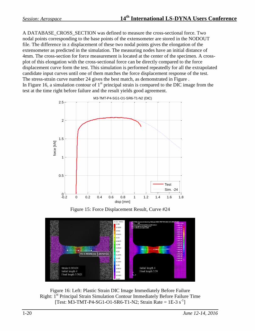
A DATABASE_CROSS_SECTION was defined to measure the cross-sectional force. Two

nodal points corresponding to the base points of the extensometer are stored in the NODOUT

file. The difference in z displacement of these two nodal points gives the elongation of the

extensometer as predicted in the simulation. The measuring nodes have an initial distance of

4mm. The cross-section for force measurement is located at the center of the specimen. A cross-

plot of this elongation with the cross-sectional force can be directly compared to the force

displacement curve form the test. This simulation is performed repeatedly for all the extrapolated

candidate input curves until one of them matches the force displacement response of the test.

The stress-strain curve number 24 gives the best match, as demonstrated in Figure .

In Figure 16, a simulation contour of 1st principal strain is compared to the DIC image from the

test at the time right before failure and the result yields good agreement.

-0.2 0 0.2 0.4 0.6 0.8 1 1.2 1.4 1.6 1.80

0.5

1

1.5

2


disp [mm]

forc

e [

kN

]

Test

Sim. -24

Figure 15: Force Displacement Result, Curve #24

Figure 16: Left: Plastic Strain DIC Image Immediately Before Failure

Right: 1st Principal Strain Simulation Contour Immediately Before Failure Time

[Test: M3-TMT-P4-SG1-O1-SR6-T1-N2; Strain Rate = 1E-3 s-1

]

14th


June 12-14, 2016 1-21

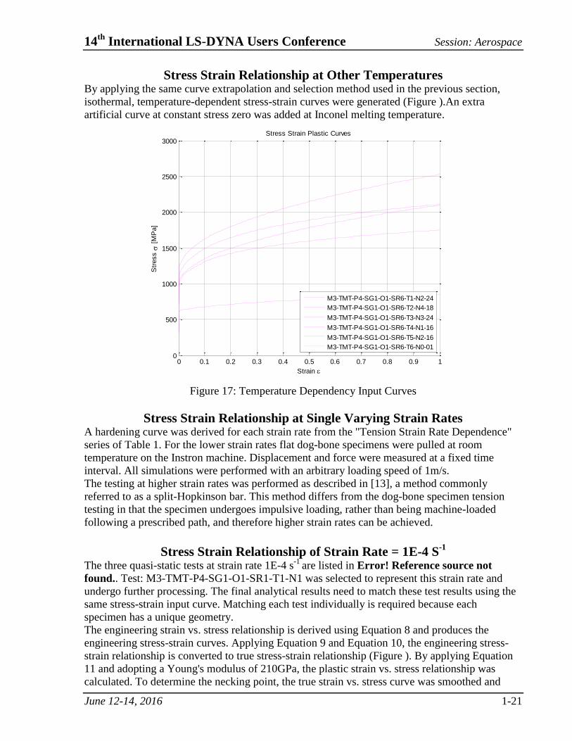
Stress Strain Relationship at Other Temperatures By applying the same curve extrapolation and selection method used in the previous section,

isothermal, temperature-dependent stress-strain curves were generated (Figure ).An extra

artificial curve at constant stress zero was added at Inconel melting temperature.

0 0.1 0.2 0.3 0.4 0.5 0.6 0.7 0.8 0.9 10

500

1000

1500

2000

2500

3000Stress Strain Plastic Curves

Strain

Str

ess

[M

Pa]

M3-TMT-P4-SG1-O1-SR6-T1-N2-24






Figure 17: Temperature Dependency Input Curves

Stress Strain Relationship at Single Varying Strain Rates A hardening curve was derived for each strain rate from the "Tension Strain Rate Dependence"

series of Table 1. For the lower strain rates flat dog-bone specimens were pulled at room

temperature on the Instron machine. Displacement and force were measured at a fixed time

interval. All simulations were performed with an arbitrary loading speed of 1m/s.

The testing at higher strain rates was performed as described in [13], a method commonly

referred to as a split-Hopkinson bar. This method differs from the dog-bone specimen tension

testing in that the specimen undergoes impulsive loading, rather than being machine-loaded

following a prescribed path, and therefore higher strain rates can be achieved.

Stress Strain Relationship of Strain Rate = 1E-4 S-1

The three quasi-static tests at strain rate 1E-4 s

-1 are listed in Error! Reference source not

found.. Test: M3-TMT-P4-SG1-O1-SR1-T1-N1 was selected to represent this strain rate and

undergo further processing. The final analytical results need to match these test results using the

same stress-strain input curve. Matching each test individually is required because each

specimen has a unique geometry.

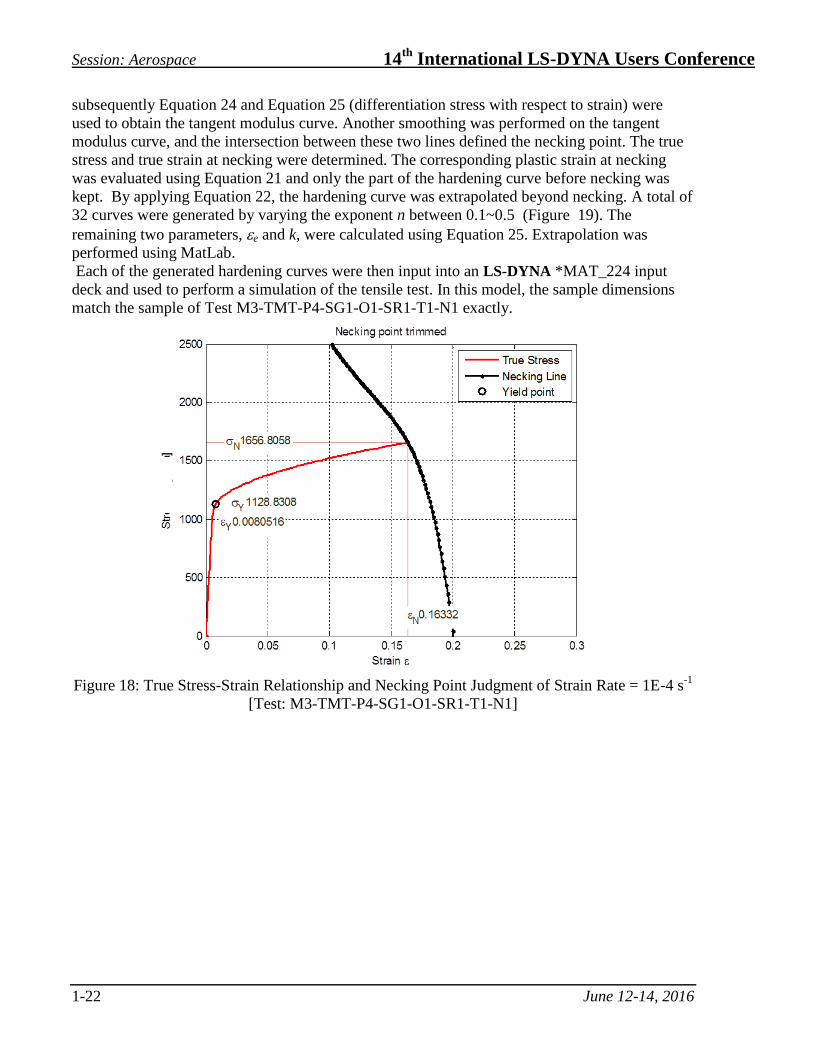
The engineering strain vs. stress relationship is derived using Equation 8 and produces the

engineering stress-strain curves. Applying Equation 9 and Equation 10, the engineering stress-

strain relationship is converted to true stress-strain relationship (Figure ). By applying Equation

11 and adopting a Young's modulus of 210GPa, the plastic strain vs. stress relationship was

calculated. To determine the necking point, the true strain vs. stress curve was smoothed and



1-22 June 12-14, 2016

subsequently Equation 24 and Equation 25 (differentiation stress with respect to strain) were

used to obtain the tangent modulus curve. Another smoothing was performed on the tangent

modulus curve, and the intersection between these two lines defined the necking point. The true

stress and true strain at necking were determined. The corresponding plastic strain at necking

was evaluated using Equation 21 and only the part of the hardening curve before necking was

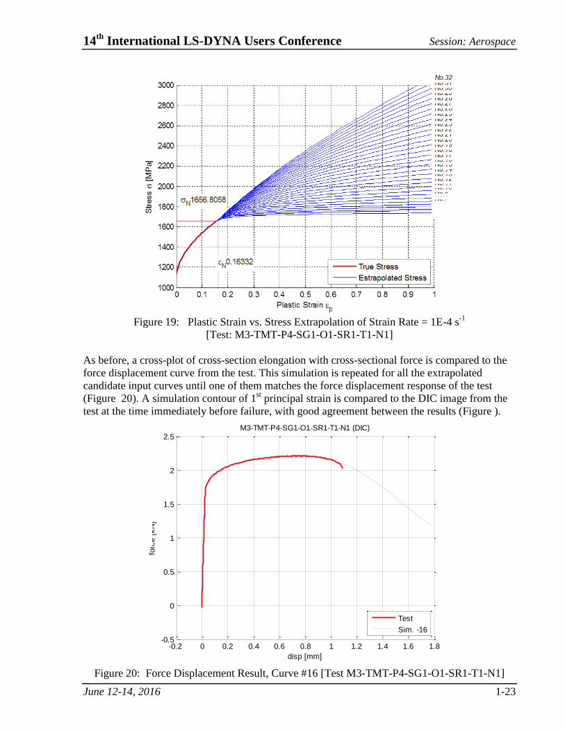
kept. By applying Equation 22, the hardening curve was extrapolated beyond necking. A total of

32 curves were generated by varying the exponent n between 0.1~0.5 (Figure 19). The

remaining two parameters, e and k, were calculated using Equation 25. Extrapolation was

performed using MatLab.

Each of the generated hardening curves were then input into an LS-DYNA *MAT_224 input

deck and used to perform a simulation of the tensile test. In this model, the sample dimensions

match the sample of Test M3-TMT-P4-SG1-O1-SR1-T1-N1 exactly.

Figure 18: True Stress-Strain Relationship and Necking Point Judgment of Strain Rate = 1E-4 s

-1

[Test: M3-TMT-P4-SG1-O1-SR1-T1-N1]

14th


June 12-14, 2016 1-23

Figure 19: Plastic Strain vs. Stress Extrapolation of Strain Rate = 1E-4 s

-1


As before, a cross-plot of cross-section elongation with cross-sectional force is compared to the

force displacement curve from the test. This simulation is repeated for all the extrapolated

candidate input curves until one of them matches the force displacement response of the test

(Figure 20). A simulation contour of 1st principal strain is compared to the DIC image from the

test at the time immediately before failure, with good agreement between the results (Figure ).

-0.2 0 0.2 0.4 0.6 0.8 1 1.2 1.4 1.6 1.8-0.5

0

0.5

1

1.5

2


disp [mm]

forc

e [

kN

]

Test

Sim. -16

Figure 20: Force Displacement Result, Curve #16 [Test M3-TMT-P4-SG1-O1-SR1-T1-N1]



1-24 June 12-14, 2016

Figure 21: Left: Plastic Strain DIC Image Immediately Before Failure

Right: 1st Principal Strain Simulation Contour Immediately Before Failure

[Test 1: M3-TMT-P4-SG1-O1-SR1-T1-N1; Strain Rate = 1E-4 s-1

]

Stress Strain Tabulated Input of Multiple Strain Rates and Temperatures The typical method for creating the higher strain rate curves using each high rate test, one at a

time, was not feasible with Inconel-718. The *MAT_224 input curves in the iso-rate table must

be at constant temperature and at a constant strain rate. Neither of these conditions was satisfied

by the Inconel-718 tests, as explained previously. Also as explained before, the process

employed for creating the higher rate stress-strain curves required combining information from

higher rate compression tests with lower, constant strain rate tension tests. An iso-thermal

constant strain rate curve needs to be used as a base-line for the synthetic high strain rate

hardening curves. The stress-strain curve at the strain rate of 1E-4 s-1

was used as the base-line in

the iso-rate table, with an off-set appropriate to match the strain rate sensitivity curve. A trial-

and-error process was performed, wherein both the magnitude of the stresses in the transition and

higher strain rate regions, and the Taylor-Quinney coefficient, β, were varied simultaneously.

Each of the tests was analyzed multiple times, until a satisfactory match to all of the test data was

achieved. Many iterations were performed before this satisfactory match was achieved. (Note

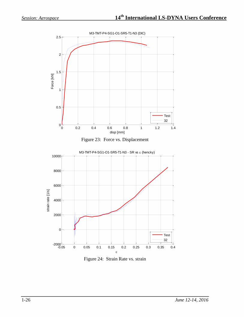
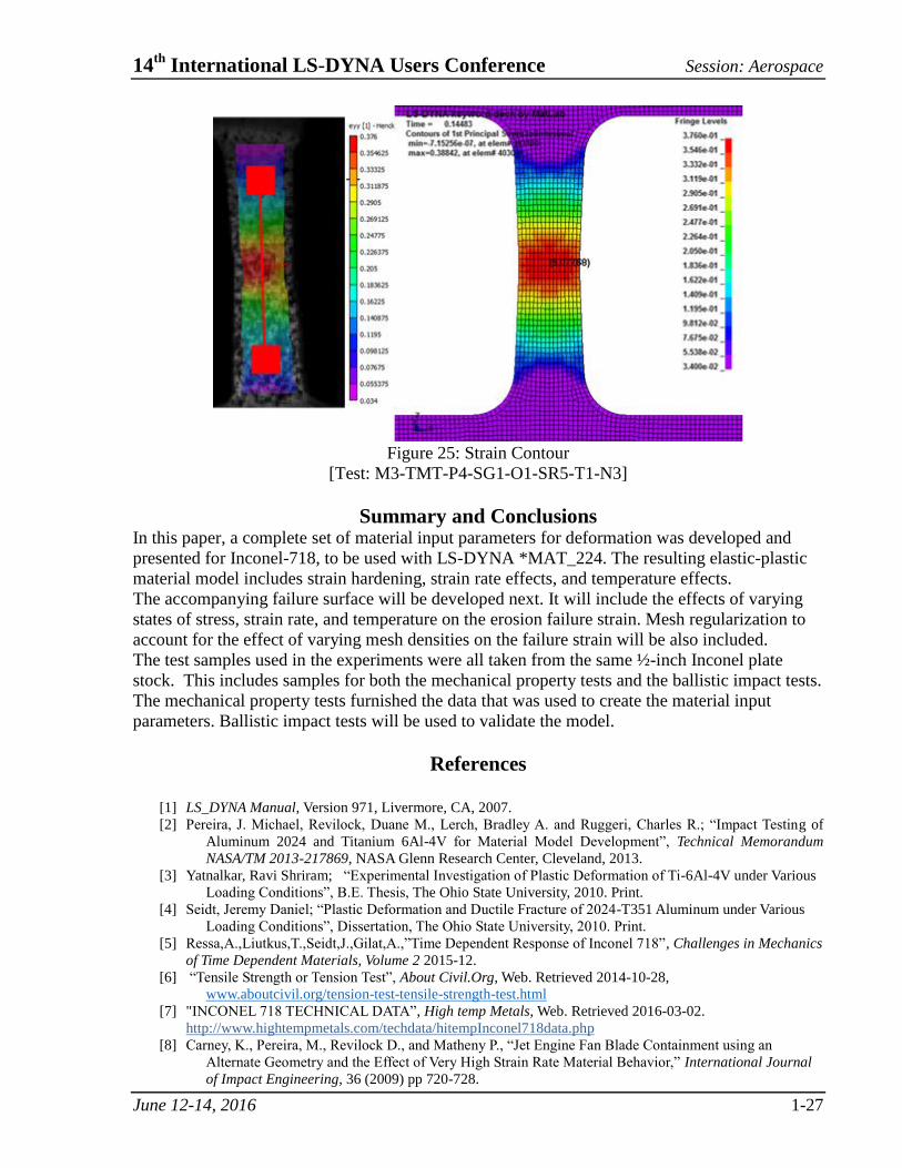
that in Figures 23 and 24 the curve labeled 32 refers both to the simulation using the final strain

rate sensitivity curve, and that 32 iterations were required before a match to all test data was

achieved.)

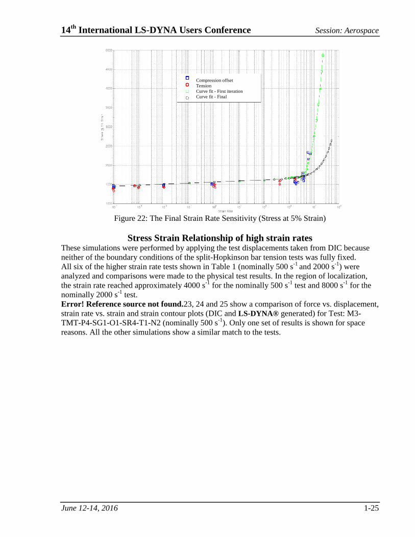
The initial and final strain rate sensitivity curve, used to offset the base stress-strain curves,

resulting from the trial-and-error process is shown in Figure 22. The final strain rate sensitivity

curve shown was used to offset the base curve and to create all the iso-rate and iso-thermal input

curves. Force vs. displacement, strain rate vs. strain and plastic strain DIC Image vs. principal

strain rate from the simulations were also used for comparison between simulations and tests.

14th


June 12-14, 2016 1-25

Figure 22: The Final Strain Rate Sensitivity (Stress at 5% Strain)

Stress Strain Relationship of high strain rates These simulations were performed by applying the test displacements taken from DIC because

neither of the boundary conditions of the split-Hopkinson bar tension tests was fully fixed.

All six of the higher strain rate tests shown in Table 1 (nominally 500 s-1

and 2000 s-1

) were

analyzed and comparisons were made to the physical test results. In the region of localization,

the strain rate reached approximately 4000 s-1

for the nominally 500 s-1

test and 8000 s-1

for the

nominally 2000 s-1

test.

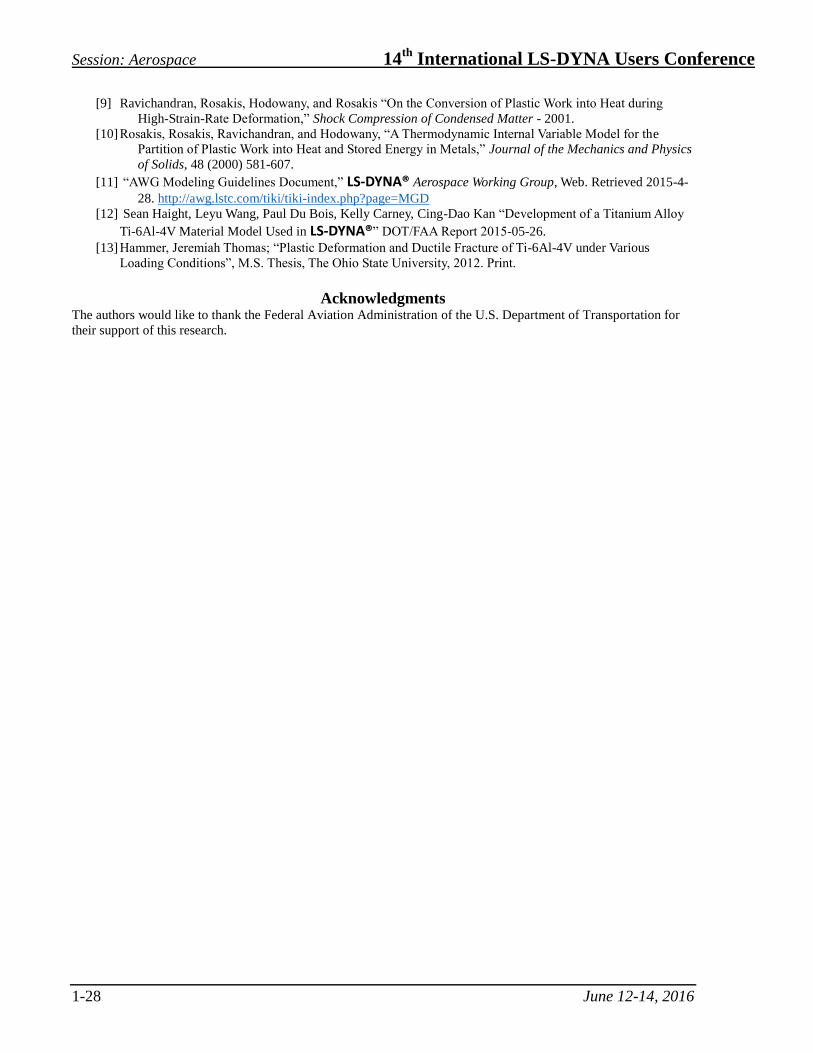
Error! Reference source not found.23, 24 and 25 show a comparison of force vs. displacement,

strain rate vs. strain and strain contour plots (DIC and LS-DYNA® generated) for Test: M3-

TMT-P4-SG1-O1-SR4-T1-N2 (nominally 500 s-1

). Only one set of results is shown for space

reasons. All the other simulations show a similar match to the tests.

Compression offset

Tension

Curve fit - First iteration

Curve fit - Final



1-26 June 12-14, 2016

0 0.2 0.4 0.6 0.8 1 1.2 1.40

0.5

1

1.5

2


disp [mm]

Forc

e [

kN

]

Test

32

Figure 23: Force vs. Displacement

-0.05 0 0.05 0.1 0.15 0.2 0.25 0.3 0.35 0.4-2000

0

2000

4000

6000

8000

10000M3-TMT-P4-SG1-O1-SR5-T1-N3 - SR vs (hencky)

str

ain

rate

[1/s

]

Test

32

Figure 24: Strain Rate vs. strain

14th


June 12-14, 2016 1-27

Figure 25: Strain Contour


Summary and Conclusions In this paper, a complete set of material input parameters for deformation was developed and

presented for Inconel-718, to be used with LS-DYNA *MAT_224. The resulting elastic-plastic

material model includes strain hardening, strain rate effects, and temperature effects. The accompanying failure surface will be developed next. It will include the effects of varying

states of stress, strain rate, and temperature on the erosion failure strain. Mesh regularization to

account for the effect of varying mesh densities on the failure strain will be also included. The test samples used in the experiments were all taken from the same ½-inch Inconel plate

stock. This includes samples for both the mechanical property tests and the ballistic impact tests.

The mechanical property tests furnished the data that was used to create the material input

parameters. Ballistic impact tests will be used to validate the model.

References

[1] LS_DYNA Manual, Version 971, Livermore, CA, 2007.

[2] Pereira, J. Michael, Revilock, Duane M., Lerch, Bradley A. and Ruggeri, Charles R.; “Impact Testing of

Aluminum 2024 and Titanium 6Al-4V for Material Model Development”, Technical Memorandum

NASA/TM 2013-217869, NASA Glenn Research Center, Cleveland, 2013.

[3] Yatnalkar, Ravi Shriram; “Experimental Investigation of Plastic Deformation of Ti-6Al-4V under Various

Loading Conditions”, B.E. Thesis, The Ohio State University, 2010. Print.

[4] Seidt, Jeremy Daniel; “Plastic Deformation and Ductile Fracture of 2024-T351 Aluminum under Various

Loading Conditions”, Dissertation, The Ohio State University, 2010. Print.

[5] Ressa,A.,Liutkus,T.,Seidt,J.,Gilat,A.,”Time Dependent Response of Inconel 718”, Challenges in Mechanics

of Time Dependent Materials, Volume 2 2015-12.

[6] “Tensile Strength or Tension Test”, About Civil.Org, Web. Retrieved 2014-10-28,

www.aboutcivil.org/tension-test-tensile-strength-test.html

[7] "INCONEL 718 TECHNICAL DATA”, High temp Metals, Web. Retrieved 2016-03-02.

http://www.hightempmetals.com/techdata/hitempInconel718data.php

[8] Carney, K., Pereira, M., Revilock D., and Matheny P., “Jet Engine Fan Blade Containment using an

Alternate Geometry and the Effect of Very High Strain Rate Material Behavior,” International Journal

of Impact Engineering, 36 (2009) pp 720-728.

http://www.aboutcivil.org/tension-test-tensile-strength-test.html



1-28 June 12-14, 2016

[9] Ravichandran, Rosakis, Hodowany, and Rosakis “On the Conversion of Plastic Work into Heat during

High-Strain-Rate Deformation,” Shock Compression of Condensed Matter - 2001.

[10] Rosakis, Rosakis, Ravichandran, and Hodowany, “A Thermodynamic Internal Variable Model for the

Partition of Plastic Work into Heat and Stored Energy in Metals,” Journal of the Mechanics and Physics

of Solids, 48 (2000) 581-607.

[11] “AWG Modeling Guidelines Document,” LS-DYNA® Aerospace Working Group, Web. Retrieved 2015-4-

28. http://awg.lstc.com/tiki/tiki-index.php?page=MGD

[12] Sean Haight, Leyu Wang, Paul Du Bois, Kelly Carney, Cing-Dao Kan “Development of a Titanium Alloy

Ti-6Al-4V Material Model Used in LS-DYNA®” DOT/FAA Report 2015-05-26.

[13] Hammer, Jeremiah Thomas; “Plastic Deformation and Ductile Fracture of Ti-6Al-4V under Various

Loading Conditions”, M.S. Thesis, The Ohio State University, 2012. Print.

Acknowledgments The authors would like to thank the Federal Aviation Administration of the U.S. Department of Transportation for

their support of this research.

http://awg.lstc.com/tiki/tiki-index.php?page=MGD

incorporation of inconel-718 material test data into

Documents