increased thermal robustness of turbine...
TRANSCRIPT

Department of Product and Production Development
CHALMERS UNIVERSITY OF TECHNOLOGY
Gothenburg, Sweden 2014
Increased Thermal Robustness of
Turbine Structure
Master´s thesis in Product Development
MATTIAS LARSSON
SEBASTIAN MARKLUND

II

III
Increased Thermal Robustness of
Turbine Structure
MATTIAS LARSSON
SEBASTIAN MARKLUND
Department of Product and Production Development
CHALMERS UNIVERSITY OF TECHNOLOGY
Gothenburg, Sweden 2014

IV
Increased Thermal Robustness of Turbine Structure
MATTIAS LARSSON
SEBASTIAN MARKLUND
© Mattias Larsson, Sebastian Marklund, 2014
Master´s Thesis
Department of Product & Production Development
Division of Product Development
Chalmers University of Technology
SE-41296 Gothenburg
Sweden
Phone +46 31 772 1000
Cover:
The Turbine Structure (Aerospace, 2014)
Chalmers Reproservice
Gothenburg, Sweden 2014

V
Increased Thermal Robustness of Turbine Structure
Master´s Thesis in Product Development
MATTIAS LARSSON
SEBASTIAN MARKLUND
Department of Product & Production Development
Division of Product Development
Chalmers University of Technology
SE-41296 Gothenburg
Sweden
Abstract
This report is a result of the master´s thesis work carried out in corporation with GKN
Aerospace Engine Systems in Trollhättan, Sweden and the department program at Chalmers
University of Technology in Gothenburg, Sweden, during the spring of 2014.
During the development of a jet engine, changes on the system level can have a great impact
on components manufactured by GKN. In previously developed jet engines it has been found
that increased temperatures have shortened the life span of the Turbine Structure, this due to a
design that is sensitive to thermal variation.
In this thesis a method for identification and reduction of sensitivity to thermal variation is
developed. The methods investigated are based on Robust Design theory and statistical
models. Design of Experiments is used for investigating how variance in the thermal zones is
affecting the stress levels in the TS.
To be able to withstand changes in thermal loads, statistical methods have been investigated
and implemented in order to design aerospace engine components towards an increased
thermal robustness.
The TS was divided into four thermal zones that were varied according to different
experimental design plans. A Taguchi L9 experimental plan was carried out and all
combinations of the varied temperature inputs were simulated in ANSYS to achieve the
corresponding temperatures in the thermal zones. These temperatures were then used as input
to the structural simulation that shows corresponding stresses in the TS.
The Design of Experiment results showed that main effects derive from the thermal zones 2
and 3. Geometrical variations together with variation in thermal boundary conditions were
also studied to determine what the most sensitive geometrical parameters were. With the
correct set up of experimental design and statistical methods, further investigation on the
geometry impact of thermal variation can be studied.
A methodology regarding analysis of Design of Experiment data was established throughout
this thesis work. Procedures for automated investigation of areas of interest were evaluated as
support for more efficient analysis of thermal robustness.

VI
Acknowledgements
This report is a result of the master thesis work made by Mattias Larsson and Sebastian
Marklund at the Department of Product and Production Development at Chalmers University
of Technology. We wish to thank our supervisors, Dr. Johan Lööf at GKN Aerospace and
Associate Professor Lars Lindkvist at Chalmers University of Technology. Their assistance in
form of planning and revising supported this project to stay on track to reach the set up goals.
Without the expertise and dedication from GKN employees this thesis had not been able to
reach the highly valued results. We especially want to thank Carlos Arroyo for his excellence
in aerothermodynamics engineering that helped and supported the work throughout the whole
project. Carlos constructed the foundation that made this work possible.
We also want to thank Richard Sävenå and Visakha Raja for their brilliance in solid
mechanics engineering. This thesis work was made possible only with Richard’s and
Visakha’s knowledge, help in programming and help with simulation setup.
Finally we want to thank Petter Andersson for his guidance throughout this work, with the
support in interpreting the data and set up of statistical aids.
Gothenburg, 2014
Mattias Larsson & Sebastian Marklund

1
Table of contents
Explanation to abbreviations ....................................................................................................................................... 4
1. Introduction .................................................................................................................................................................... 5
1.2 Company Description .......................................................................................................................................... 5
1.3 Background ............................................................................................................................................................. 6
1.4 Purpose and Aim ................................................................................................................................................... 7
1.5 Research questions .............................................................................................................................................. 7
1.6 Delimitations .......................................................................................................................................................... 8
1.7 Secrecy ...................................................................................................................................................................... 8
1.8 Structure of the report ........................................................................................................................................ 9
2. Theory ............................................................................................................................................................................. 10
2.1 Jet engine functionality ..................................................................................................................................... 10
2.2 Turbine Structure ............................................................................................................................................... 12
2.3 Thermal management ....................................................................................................................................... 13
2.3.1 Conduction .................................................................................................................................................... 13
2.3.2 Convection ..................................................................................................................................................... 13
2.3.3 Radiation ........................................................................................................................................................ 14
2.3.4 Thermal expansion .................................................................................................................................... 14
2.4 Robust Design Methods .................................................................................................................................... 15
2.4.1 Robust Design .............................................................................................................................................. 15
2.4.2 Taguchi method .......................................................................................................................................... 16
2.5 Experimental design .......................................................................................................................................... 17
2.5.1 Design of Experiment ............................................................................................................................... 17
2.5.2 Design of Experiments methodologies .............................................................................................. 20
2.5.3 Taguchi Methods ........................................................................................................................................ 25
2.6 Response surface methodology .................................................................................................................... 29
2.6.1 Neural Network Function ....................................................................................................................... 30
2.7 Regression theory ............................................................................................................................................... 31
2.8 Statistical correlation ........................................................................................................................................ 32
2.9 Analysis of variance (ANOVA) ....................................................................................................................... 33
2.9.1 Verification and Validation ..................................................................................................................... 34
2.9.2 Fischer F-test ................................................................................................................................................ 34

2
2.9.3 P-Value ............................................................................................................................................................ 34
2.10 Selection of Experimental Design .............................................................................................................. 36
3. Method ............................................................................................................................................................................ 37
3.1 Literature studies ............................................................................................................................................... 37
3.2 Data Acquisition .................................................................................................................................................. 37
3.4 Development process ........................................................................................................................................ 38
3.5 Thermal analysis ................................................................................................................................................. 39
3.6 Structural analysis .............................................................................................................................................. 39
3.7 Post processing of simulation data and use of statistical methods ................................................ 40
3.8 Geometrical variation ....................................................................................................................................... 40
4. Results ............................................................................................................................................................................. 41
4.1 Selection of process parameters ................................................................................................................... 41
4.2 Thermal Management ....................................................................................................................................... 42
4.3 Experimental plan .............................................................................................................................................. 44
4.4 Positioning of nodes .......................................................................................................................................... 45
4.5 Simulation setup ................................................................................................................................................. 46
4.6 Temperature and stress distributions ....................................................................................................... 48
4.6.1 Thermal distribution ................................................................................................................................. 48
4.6.2 Stress distributions.................................................................................................................................... 48
4.7 Analysis of the results ....................................................................................................................................... 49
4.8 Scatter plots .......................................................................................................................................................... 50
4.9 Normal probability plot ................................................................................................................................... 51
4.10 Temperature gradient plots......................................................................................................................... 52
4.11 Main effects plots ............................................................................................................................................. 54
4.12 Effect of thermal zones .................................................................................................................................. 56
4.13 Correlation .......................................................................................................................................................... 58
4.14 Response surface methodology ................................................................................................................. 58
4.14.1 Analysis of Variance................................................................................................................................ 59
4.14.2 Linear model .............................................................................................................................................. 60
4.14.3 Interaction model .................................................................................................................................... 61
4.14.4 Purequadratic model .............................................................................................................................. 62
4.14.5 Quadratic model ....................................................................................................................................... 63
4.15 Box-Behnken setup ......................................................................................................................................... 67
4.16 Geometry variation.......................................................................................................................................... 70
4.16.1 Interpolated nodes .................................................................................................................................. 70

3
4.16.2 Determining sensitive parameters ................................................................................................... 71
4.16.4 Robustness plots ...................................................................................................................................... 72
5. Discussion ...................................................................................................................................................................... 74
5.1 Improvement of analysis procedure ........................................................................................................... 75
6. Sources of error........................................................................................................................................................... 77
7. Conclusion ..................................................................................................................................................................... 78
8. Developed methodology for investigation of thermal robustness ........................................................ 80
9. Further work ................................................................................................................................................................ 81
10. References .................................................................................................................................................................. 83
Appendix I .......................................................................................................................................................................... 86
Appendix II......................................................................................................................................................................... 87
Appendix III ....................................................................................................................................................................... 88
Appendix IV ....................................................................................................................................................................... 89
Appendix V ......................................................................................................................................................................... 90

4
Explanation to abbreviations
EWB – Engineering Workbench
NTL – Newton’s Third Law of motion
LPC – Low Pressure Compressor
HPC – High Pressure Compressor
LPT – Low Pressure Turbine
HPT – High Pressure Turbine
TS – Turbine Structure
TBH – Tail Bearing Housing
TRF – Turbine Rear Frame
BC – Boundary Condition
DoE – Design of Experiments
DoF – Degrees of Freedom
GKN – GKN Aerospace Engine Systems
ANSYS – Fluid dynamics and solid mechanics simulation software
MATLAB – Mathematical and statistical software
MINITAB – Statistical software
LE – Leading Edge
TE – Trailing Edge
ModeFrontier – Multi-objective optimization software
CUMFAT – Analysis for determination of component life and fatigue

5
1. Introduction
This introductory chapter presents GKN together with the description of the background and
current situation to the problem area. The introduction also explains the purpose of this thesis
and its goal definitions. A description of the limitations and structure of the thesis report are
also presented.
1.2 Company Description
GKN Aerospace Sweden AB is the parent company for the division GKN Aerospace Engine
Systems within the GKN Group. GKN Aerospace serves a global customer base and operates
in Europe and North America. The company is one of the world´s independent tier supplier to
the global aviation industry, with GKN as a global leader in the aero structures and engine
components manufacturing for both the military and civil market. With over 100 years of
aerospace experience, extensive knowledge utilization and advanced manufacturing
technologies, GKN delivers high-valuable integrated assemblies in both metallic and
composite materials. (Aerospace, 2014)
The company has approximately 12 000 employees distributed in more than 35 facilities
across four continents. The GKN Aerospace AB headquarters is located in Trollhättan, where
manufacturing of engine components and the development of the Turbine Structure is taking
place.
GKNs vision and goals are to get an even broader range of product families within the core
structures, engine assemblies, transparencies and niche technology markets. The design and
manufacture of high level integrated aircraft assemblies and sub-assemblies for OEM´s and
Tier One customers. Finally GKN strives for an expansion into adjacent markets with similar
product technologies and manufacturing capabilities. (Aerospace, 2014)
“GKN Aerospace is committed to being the best value solution for our customers worldwide
to meet aerospace and defense needs” (Aerospace, 2014)

6
1.3 Background
In the modern world with an increasingly extensive global competitive market, shortened lead
times in product developments is not only a recommendation, it is a vital key for success. The
development time reflects how responsive the company can be to competitive forces and
technological developments. It also tells how quickly the company receives the economic
returns from the project´s resource and time efforts (Ulrich, 2011).
During the development of a jet engine, changes on the system level can have a great impact
on components manufactured by GKN. Due to aim of shortened lead times the need of early
decisions in the development phase are of great importance. The resulting costs of changes in
the development phase are heavily dependent on in which part of the progress stage the
changes are made. Changes made at an early stage in the development phase are substantially
more affordable than major changes made late in the process, which often result in an
exponentially increased total cost for implementation of the new procedures.
In previously developed jet engines it has been found that increased temperatures have
shortened the life span of the TS and this due to a design that is sensitive to thermal variation.
To be able to withstand changes in thermal loads, statistical methods need to be incorporated
in order to design aerospace engine components towards an increased thermal robustness. To
gain thermal robustness it is important to explore alternative design configurations with
respect to thermal uncertainties. In negotiation with GKN customers there is a need for
engineering know how, trade off curves etc. as support, when providing powerful arguments
in new engine programs. To account for these challenges there is a demand to develop robust
methods and simulation support in early phases of the product development cycle.
As a part of decreasing lead times in product development at GKN and to make the product
development processes more effective the company has started a work team called
Engineering Workbench, hereafter called (EWB). EWBs´ main function is to create a cross
functional team from different engineering disciplines. EWD also supports a more effective
exchange of important information across the engineering disciplines at GKN.
7
1.4 Purpose and Aim
As described in the previous chapter the urge for early decision making in the development
process is a key factor for success in the modern global competitive market. This quest for
early decision making requires that the decisions are based on facts, which in turn has to be
based on qualitative available information. To gain this important information at an early
stage in the innovation process reliable and effective methods are invaluable. One important
part of this thesis is to explore the possibilities for implementation of these methodologies to
gain valuable knowledge at an early stage in the development process. This research is closely
connected to the improvement capabilities of the EWB group at GKN.
The purpose of this thesis is to explore and understand what impact a variation in boundary
conditions has on important design properties in the development phase. A methodology is
needed for identifying sensitive parameters and how variation in boundary conditions is
treated. The task is to define possible methods and tools that should be used to improve
engineering efficiency and utilization of statistical tools to decrease sensitivity on GKN
developed components when changes are made on the system level on the TS.
Definition of a set-based approach is needed in order to get knowledge about how robust the
TS are to changes made on the system level. The thesis should result in a more engineering
efficient way to handle variations in boundary conditions and parameters in early
development phases.
1.5 Research questions
This thesis will regard the following three research questions. The outline of the thesis is
based on these questions.
1. How to identify key design parameters that are coupled to thermal variation?
This research question will address how key design parameters can be identified and
how these are treated during the ongoing development project.
2. How is it possible to in an efficient way handle variations in key design
parameters during ongoing development projects?
This question will address how a methodological approach can be implemented to
obtain a robust design with respect to thermal and geometric attributes.
3. How can Design of Experiments (DoE) be implemented to improve thermal
robustness in an early phase of the development project?
This question will address how design of experiment can be implemented in
multidisciplinary simulations in order to improve thermal robustness in early stages of
product development.

8
1.6 Delimitations
Limited resources in terms of time, budget and knowledge makes it necessary to establish
boundaries of the thesis project performed at GKN. Research will be done on one single
component in the engine, the TS, and not additional parts of the engine. Examination and
analysis will be made on already existing models at GKN. Tests and implementations will not
be evaluated and examined through an economical point of view. Delimitations will also be
done to only include those parameters that affect the investigated component. Also the
investigation should be on a low level of detail in the component, with only the most
important parameters included for observation. Some geometric features are also fixed and
should not be taken into consideration when investigating variation of geometric parameters.
The mentioned features will be described at a later stage. The tools and methods used are
limited to the software and tools available at GKN.
1.7 Secrecy
Due to secrecy reasons the authors of this report are bound to follow laws and regulations
under confidentiality agreement with GKN. For this reason, results and conclusions have been
removed in the public version of this thesis. Data has been normalized, figures are modified,
reduced in quantity and names of variables have been changed. Valid results are given in the
internal report available at GKN.

9
1.8 Structure of the report
The structure of this thesis report is outlined in a scientific format referred to Chalmers
standard form for master thesis reports. The report will be subdivided into the following
sections.
Chapter 1. Provides a presentation of GKN Aerospace Engine systems and the description
of the relevant problem which is the basis for this master thesis. The goal and scopes for this
project are presented in terms of research questions, together with delimitations and
assumptions.
Chapter 2. Contains the introduction of jet engine theory, a description of the examined
component and the related thermal issues. This chapter also describes the tools and methods
used to succeed with the ongoing work.
Chapter 3. Explains the method of how this thesis work was carried out. The method
describes how the theory and methodologies earlier presented are meant to be implemented in
the ongoing thesis work.
Chapter 4. Presents what methodologies that were used in this master thesis and what tools
that were finally implemented. The chapter also presents the results derived from the thesis
work.
Chapter 5. Reflects on how well the results derived in this work answer the research
questions. The chapter deals with the discussion about the generated results, and debates
about how relevant the findings are in an engineering manner.
Chapter 6. Presents the sources of error that was found throughout the thesis work.
Chapter 7. Presents the conclusions drawn from the derived results of this thesis work.
Chapter 8. Presents the developed methodology that is to be used when investigating thermal
robustness.
Chapter 9. Presents future work that can be followed by this thesis work.
Chapter 10. Presents the list of references
Chapter 11. List of all appendices.

10
2. Theory
This chapter contains the introduction of jet engine theory, a description of the examined
component and the related thermal issues. It also describes the tools and methods used to
succeed with the ongoing work.
2.1 Jet engine functionality
The imminent majority of today’s commercial airplanes use jet engine propulsion. “Jet
engine” is a broad definition of a variety of engines using Newton’s laws of motion saying
that for every action of force there is an equal and opposite reaction force. Jet engine, in
common parlance, may also be referring to as “internal combustion air breathing jet engine”.
In a jet engine air is accelerated through the engine and gives the air a change in momentum.
From NTL this translates to the thrust equation
𝐹 = ṁ(𝑉0 − 𝑉1) (2.1)
Where ṁ is the mass flow rate of air and V0,1 is the relative speed before and after the jet
engine. From this it is also clear that the purpose of the engine is to produce large volumes of
exhaust gasses that move at high velocity. Figure 2.1 below shows a basic view over a civil
bypass jet engine. Air first enters the front facing fan that sucks in air to feed the compressors.
The airstream enters the low pressure compressor (LPC). In this stage the larger quantity of
air enters the bypass canal for direct thrust. Small volumes of air, typically around 10%
depending on engine set-up, enter the jet engine core for later ignition. After the LPC the air
is further compressed in the high pressure compressor (HPC) to a stage where the pressure
ratio is between 20:1 and 80:1, much depending on how many stages of blades that is present
in the first two compressor stages.
Figure 2.1. PW1000G jet engine sectors.

11
To overcome the aerodynamic drag of an airplane the thrust needs to be larger than the
aerodynamic drag. The compressor raises the pressure of the incoming air and forces the air
towards the combustion chamber. To create a higher velocity of the exhaust gasses fuel is
mixed with the compressed air in the combustion system and a light spark ignites the air-fuel
mixture. The ignited fuel mixture then expands with high pressure and accelerates through the
turbines of the engine. A fraction of this energy is used to produce thrust. The hot gasses from
the combustor enter the high pressure turbine (HPT), and the HPT extracts the energy
produced in the combustor by transforming the energy to kinetic energy. In the same way as
the compressor, the turbine consists of rotating discs of blades and static vanes. Turbine
blades transform the pressurized stream of gasses from the combustion into kinetic energy
that is used to produce thrust and compression. In a two-axial bypass engine the kinetic
energy from the HPT is used for compression in the HPC. This since the HPC is mounted on
the same shaft as the HPT, see figure 2.1. After the HPT the hot gasses enter the low pressure
turbine (LPT). The LPT is mounted on the same shaft as the fan and the LPC. The extracted
energy from this stage is used to produce thrust at the fan and for compression of air in the
LPC. All of the remaining energy blows out as exhaust gasses at the exit nozzle at back of the
jet engine, but between these stages the jet stream passes the Turbine Structure (TS). The TS
is also often called tail bearing housing (TBH) or turbine rear frame (TRF) and this
component is the topic of this thesis and will explained further in the following chapters.
In a commercial jet engine the exhaust gasses only produce a small amount of thrust where
the larger proportions of thrust is produced from the fan that pushes large volumes of air
around the core of the engine into the bypass canal. This air flow is also called “by pass air”.
This configuration is optimized for the most fuel efficient flight cycle and is therefore more
fuel efficient than for example a military jet engine that demands rapid changes in altitude and
speed. In military engines all of the air from the fan enters the engine core for combustion and
all of the thrust is gained from the exhaust of these gasses. Figure 2.2 shows a common
turbojet for military purposes. This configuration on the other hand requires large volumes of
fuel, but produces larger thrust.
Figure 2.2. Cross-section view of a military jet engine.

12
2.2 Turbine Structure
This report will consider some of the problems that occur in the TS during normal operating
conditions. The TS can most easily be seen as an exhaust to the jet engine. It is mounted on
the airplane wing and carries a large proportion of the weight of the jet engine, see figure 2.3.
The part has to withstand high temperatures that arise due to exposure of hot exhaust gasses,
but also the forces from aerodynamic drag that is created when the TS redirect the jet stream
that exits the LPT. The TS also functions as a tail bearing house that holds the bearing for the
jet engine shafts and has numerous interfaces to different parts of the jet engine. Some of the
interfaces that can easily be seen are the interfaces to the LPT, the wing, the tail cone and the
bearings, but the TS also contains important hydraulic and electrical tubing as well as sensors
for the engine control system.
Figure 2.3 The Turbine Structure (TS)
In figure 2.3 a TS can be seen with a configuration of 14 struts (also called vanes) that are
used to redirect the jet stream exiting the LPT. The struts are often hollow and contain
hydraulics and electrical tubing. In some engine configurations the struts are also internally
cooled in the same way as for the turbine blades in order to reduce the temperature and
thermal expansion of the struts. The center structure consists of the hub that also provides
structural support for the rotor bearings and the hub cone. On top of the TS there are for this
engine three mount lugs that holds the engine to the airplane’s wings. The mount lugs is
placed on the outer case of the TS and the whole structure is welded together by industrial
robots.

13
2.3 Thermal management
Thermal management will in this report regard thermal zones bordering the Turbine Structure
(TS) and the thermal boundary conditions that act on the TS during operation. GKN
Aerospace has found that the TS suffer from a lowered life due to high sensitivity of low
cycle fatigue during the flight cycle. This occurs mainly when the airplane is at idle phase
between flights. During idle the temperatures exiting from the LPT increases. A simple, but
ill-considered, conclusion would be that this is the cause of the problem, but when looking
closer the problem becomes more complex. Many different cavities can found within the TS.
All of these cavities have different temperatures during the flight cycle and the temperatures
varies with changes in a range of variables such as altitude, airspeed, humidity, air
temperature, air density and thrust.
Computerized simulations can be performed in order to evaluate how a jet engine performs
during operation. Disciplines in fluid dynamics and heat transfer are used to calculate how
variations in surrounding temperatures affect stress distributions in the TS. In order to
understand the underlying processes of this phenomenon fundamental principles of heat
transfer are needed.
Heat transfer focuses on the energy transfer that occurs due to temperature gradients between
areas of different temperature levels. Heat transfer occurs as a result of three different
mechanisms, conduction, convection and radiation (Kutz, 2009).
2.3.1 Conduction
This mechanism focuses on the transfer of energy through direct contact between molecules
and therefore the transfer of energy between areas of high temperatures to the areas of lower
temperatures. A substance ability to transfer energy through conduction is represented by the
constant of thermal conductivity ĸ. The thermal conductivity varies for different materials and
is often denoted in material specifications. The fundamental relationship for heat transfer is
termed Fourier’s law of heat conduction. For a three-dimensional expression of the heat
transfer over time, the following heat diffusion equation is used (Kutz, 2009):
∂
∂x(k
∂T
∂x) +
∂
∂y(k
∂T
∂y) +
∂
∂z(k
∂T
∂z) + q = ρcp
∂
∂x
∂T
∂t (2.2)
Where cp is the specific heat capacity and ρ the density of the material. q denotes the internal
heat generation. cp and ρ are tabulated data given by material specifications.
2.3.2 Convection
This mechanism focuses on the transfer of energy that is being transferred through a motion
of a fluid. The heat transfer rate can be described by Newton’s law of cooling and is denoted:
q = hA(T1 − T2) (2.3)
Where h is the heat transfer coefficient and A is the surface area (Kutz, 2009).

14
2.3.3 Radiation
This mechanism focuses on the transfer of energy that occurs through electromagnetic waves
or through photons. The radiation mechanism is not contributory to rising temperature levels
and is not considered further.
2.3.4 Thermal expansion
When a material experiences a change in temperature, the material wants to expand due to
increased atomic vibration. The linear thermal expansion equation is written:
∆ℰ = ℰ0⍺(T1 − T0) (2.4)
Where ℰ is thermal expansion and ⍺ is the thermal expansion coefficient (Lundh, 2000). ℰ
and ⍺ are tabulated data given by material specifications. Hookes Law states that the stress is
equal to the thermal expansion multiplied with the elastic modulus E
σ = Eε (2.5)
This implies that the change in temperature raises the thermal expansion, which leads to an
increased stress level in the component.

15
2.4 Robust Design Methods This chapter describes the fundamentals of robust design and its principles. Different tools implemented in the philosophy of robust design are described.
“Validation requires documented evidence that a process consistently conforms to
requirements. It requires that you first obtain a process that can consistently conform to
requirements and then that you run studies demonstrating that this is the case. Statistical
tools can aid in both tasks.” (Taylor, 1991)
2.4.1 Robust Design
One definition of a robust process or product is the ability to perform as intended even during
non-ideal conditions. The term noise is used to describe uncontrolled variation in the process
that may affect the outcome or performance. The activity in engineering development
processes that aims at minimizing this sensitivity to uncontrolled variations that may affect
performance is called “Robust design”.
The goal is to find the combination of which parameters and what numerical values they
should range between, that generates the least sensitive to uncontrolled variation. An
experimental approach is used to find these robust points.
Figure 2.4. Well selected inputs make the output less sensitive to the variation of the input.
(Taylor, 1991)

16
As shown in figure 2.4, a more robust design results in less variation and higher quality, but
without additional costs. There exists a variety of tools for identifying key inputs and the
sources of variation. One of those is Analysis of variance (ANOVA), which is a statistical
study including statistical methods to determining if significant differences exist between
populations. (Taylor, 1991). ANOVA is further described in chapter 2.12.
Robust design methods refer to the different methods of selecting the optimal values for
inputs. As shown in figure 2.4, when nonlinear relationships exist between inputs and outputs,
a careful selection of inputs makes the outputs less sensitive to a variation in these inputs.
This means that the distribution of variation can stay the same, but with less impact on the
outputs.
2.4.2 Taguchi method
The modern robust design methodologies has its origin from the 1950s and the Japanese
engineer Genichi Taguchis ideas regarding improving quality by minimizing the negative
effects of variation, rather than trying to eliminate the variation itself.
Taguchi divides the inputs in three different categories; noise factors, signal factors and
control factors. These three inputs are all affecting the output or response. The noise factors
are representing the type of variation that is uncontrollable in the process. The relation is
shown in figure 2.5. (Forslund, 2012)
Figure 2.5. Visualizes the parameter diagram of a product, process or a system.
The utilization of noise and control factors are very suitable when it comes to investigation of
real processes. In computer simulations though the experiments are deterministic, which
means that all parameters are controllable, even the noise factors. (Forslund, 2012)

17
2.5 Experimental design
Experimental design is used to discover and examine the relationship between inputs and
output. The definition of an experimental approach is the treatment of a group of parameters
with the interest in observing the impact of the response. The construction and execution of
the experiments has of course a major impact on the credibility in the results, which makes
the validation of the experiment design extremely important.
To show the relationship between inputs and output a response surface can be used to
graphically display an estimated equation from the simulated response and thereafter be able
to predict the response from a change in input. (Ulrich, 2011)
2.5.1 Design of Experiment
This chapter will explain the methodology of Design of Experiments, hereafter also called
DoE, and its use.
Introduction to DoE
In the product development phase early decisions usually have a significant impact on later
project results. A cornerstone in a successful product development is to base decisions on
facts and making the right choices early in the concept phase. Therefore knowledge
accumulation has to be done at an early stage in the development phase but also in an
effective and rapid way. A method for gathering this early knowledge is set up of experiments
to provide information regarding important design and process parameters. The experiments
needs to be planned and executed in a structured way to achieve best possible products and
processes at the lowest cost. This form of controlled experiments gives an empirical base for
decision making when examining parameters and their effect on output results. It is also an
important tool to significantly reduce the time required for the experimental investigation.
The procedure is efficient for finding multiple parameters effect on the investigated
performance, as well to study each parameters individual to see which factor that has more or
less influence on the performance. (Ulrich, 2011)
“Design of experiments (DOE) is a systematic, rigorous approach to engineering problem-
solving that applies principles and techniques at the data collection stage so as to ensure the
generation of valid, defensible, and supportable engineering conclusions. In addition, all of
this is carried out under the constraint of a minimal expenditure of engineering runs, time,
and money.” (NIST, 2013a)
Design of Experiments is a method for assessing and quantifying the robustness in a design.
The utilization of DoE as a method for analyzing variation in design parameters is an
effective way to gain knowledge about how these parameters affect the robustness of the
product. (Aerospace, u.d.)
Statistical Design of Experiments is a method for managing variation while learning the most
from limited resources in what factors influence performance. Performing the correct DoE is
an efficient utilization of available resource to gain required knowledge. (Simpson, 2013)

18
The initial step of DoE is to determine what the objectives of the experiment plan are, and
selecting the correct parameters or factors to study. A well designed experiment plan extracts
maximum information obtained from the required experimental effort.
To better understand the fundamental properties of DoE, the different steps when developing
the design of experiment plan and the interpretation of results will be explained hereafter.
The basic structure for all DoE’s follows these seven steps:
1. Set objectives
2. Select process variables
3. Set up of experimental plan
4. Execution of the experiment design
5. Screening to find important factors
6. Analyze and interpret the results
7. Use results or repeat the process
Set objectives
This initial step defines what are the objectives are for the experiment. This question answers
what should be examined, and what kind of result that are needed to make relevant
conclusions. This is a very critical step and therefore a great understanding is required before
initiating an analysis.
Select process variables
Examine which input and output parameters that are important. This is made from a cause and
effect analysis and engineering experience. This step is very crucial for the outcome of the
DoE, where a bad choice of parameters will affect the total credibility of the results.
Set up of experimental plan
The way the experimental plan is set up depends on what the objectives is for the experiments
and what number and type of factors that will be investigated. At this step number of factors
(parameters) and how they will be varied is set up in an experimental plan matrix. Different
methods are used for varying the factors in different combinations. This will be further
explained later.
Execution of the experiment design
Run the experiments according to the set up experiment plan. Depending on the experiments
this step may be very time consuming and require a lot of resources. A well-defined
experiment plan can therefore save substantially recourses as time and costs.
Screening to find important factors
With help of the results obtained from the experiments contrasts and the effect of each factor
and its interactions will be calculated. This effect shows how strongly a variance in a certain
input parameter is affecting the output response.

19
Analyze and interpret the results
Statistical analysis needs to be done on the results to find out how likely it is that a certain
factor really influence an output. This will be further described in chapter 3.7.
Use results or repeat the process
When the results are validated and proved one can draw conclusions from the analyzed
results. Are the effects reliable and the right factors chosen, or should the experiments be
repeated with another configuration? Maybe the first set up of experiments was to discover
main effects in a screening design, and now a more in depth understanding is needed with a
design for response surface. (NIST, 2013b)
20
2.5.2 Design of Experiments methodologies
This chapter describes relevant DoE design setups and their aim.
Factorial Design
In Design of Experiments the full factorial experiment plan is method for examine two or
more parameters or “factors”, each with different set of values or “levels“. According to the
setup of the experiment plan then all possible combinations of these factors and their
interactions are examined.
The number of experiments run for a full factorial defines by the number of levels of the
factors squared by number of factors chosen, for example a two level – 4 factor design need
24 = 16 runs. All fractional designs can be expressed as the notation𝐼𝑘−𝑝 , where I is the
amount of levels for each factors, k represents the amount of factors and p the fraction of the
full factorial that is used. The term p defines the amount of generators, in other words the
number of effects and interactions that can’t be estimated entirely independent of each other.
Often a full factorial design is too comprehensive to be feasible in an economically or time
consuming perspective. Through “engineering experience” the designer can carefully choose
to remove some (often the majority) of the combinations, to make the experimental plan more
compact. (Ulrich, 2011)
When making statistical analysis of generated results from factorial experiments, the Sparsity-
Of-Effects Principle states the model often is dominated by main effects and low order
interactions. This gives that main effects and two-factor interactions will result in the most
significant responses in a factorial experiment, and the sparsity-of-effects principle actually
refers to the thought that only a few effects in a factorial experiment plan will be significant.
(Wu. C.F. Jeff, 2000)
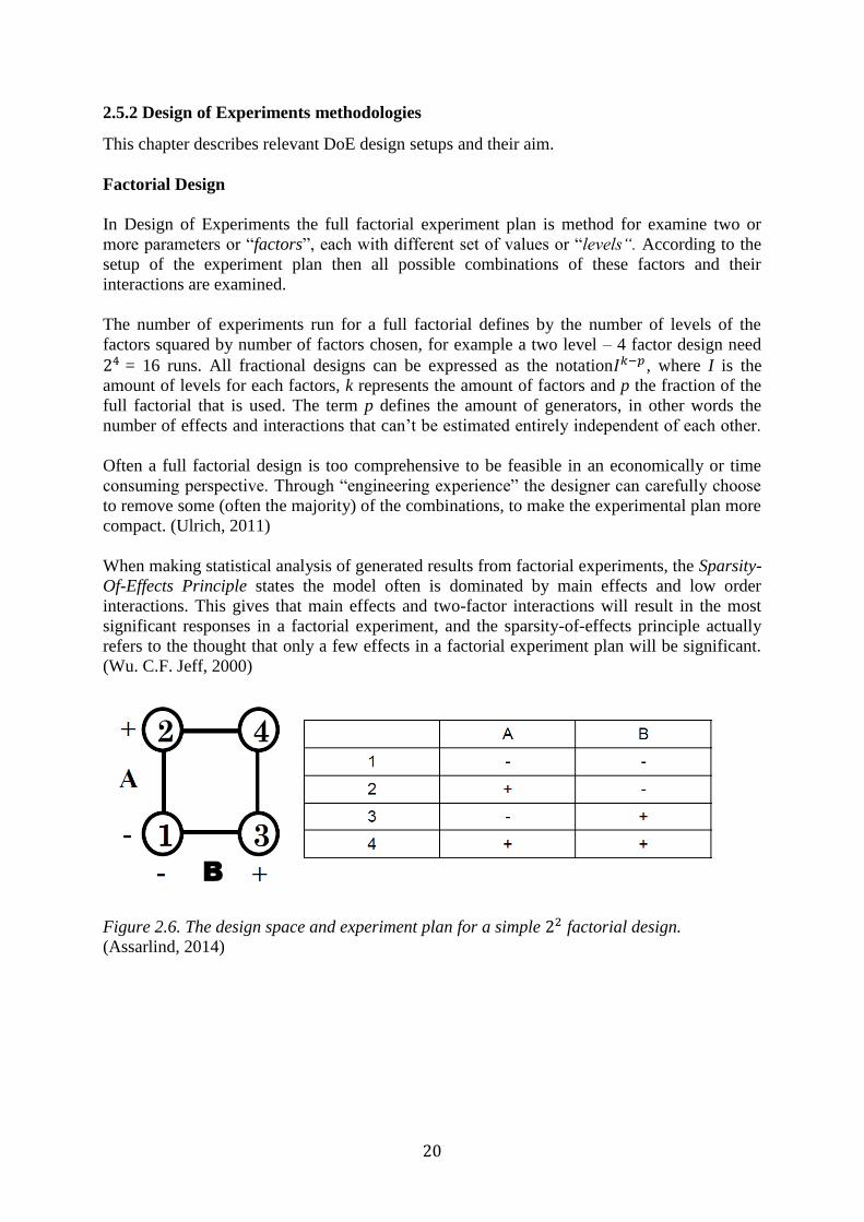
Figure 2.6. The design space and experiment plan for a simple 22 factorial design.
(Assarlind, 2014)

21
Factor effects in DoE
The main effect is the average effect of increasing the level of one factor from lower to higher
value in the design matrix. The effect corresponds to the influence that a change in level for a
certain factor has on the response. The effects are calculated as the difference between the
averages of responses when the factors are, respectively, set at higher and lower levels. The
interaction effects can be described as the effect of one factor influenced by the levels of
another factor.
The corresponding calculation of effects for both factors and their interaction for the example
in figure 2.6, are illustrated in figure 2.7;
𝑙𝐴 = 𝑦2+ 𝑦4
2 -
𝑦1+ 𝑦3
2 𝑙𝐵 =
𝑦3+ 𝑦4
2 -
𝑦1+ 𝑦2
2 𝑙𝐴𝐵 =
𝑦1+ 𝑦4
2 -
𝑦2+ 𝑦3
2 (2.6)
Figure 2.7. The corresponding effects for the two factors and their interaction.
In practice higher order levels than two is rarely used, since response surface methodology is
a more efficient way to investigate the correlation between factors and the corresponding
response. It is also hard and very inefficient to use a design for more than two levels,
compared to the response surface designs. (Assarlind, 2014)
A full saturated fractional design can investigate, at most, 2𝑛 -1 factors; for example, seven
factors needs 8 experiments.
22
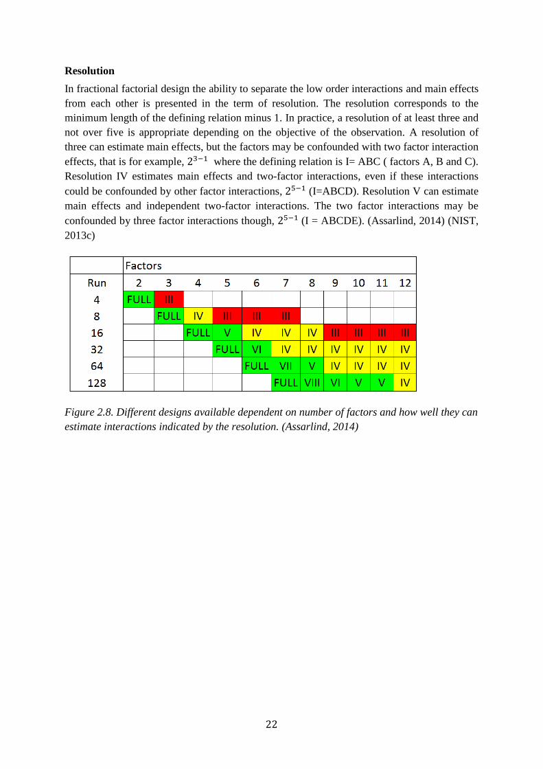
Resolution
In fractional factorial design the ability to separate the low order interactions and main effects
from each other is presented in the term of resolution. The resolution corresponds to the
minimum length of the defining relation minus 1. In practice, a resolution of at least three and
not over five is appropriate depending on the objective of the observation. A resolution of
three can estimate main effects, but the factors may be confounded with two factor interaction
effects, that is for example, 23−1 where the defining relation is I= ABC ( factors A, B and C).
Resolution IV estimates main effects and two-factor interactions, even if these interactions
could be confounded by other factor interactions, 25−1 (I=ABCD). Resolution V can estimate
main effects and independent two-factor interactions. The two factor interactions may be
confounded by three factor interactions though, 25−1 (I = ABCDE). (Assarlind, 2014) (NIST,
2013c)
Figure 2.8. Different designs available dependent on number of factors and how well they can
estimate interactions indicated by the resolution. (Assarlind, 2014)

23
Orthogonal Arrays
A correct set up factorial designs allow unbiased estimates of effects of factors and
interactions because these are orthogonal to each other. An Orthogonal design gives that the
effect of one factor is cancelled out by averaging for other factors. The cross product of the
design matrix with itself is diagonal. An example of an orthogonal design is shown in figure
4.5, in the appearance of a L9 Taguchi design.
The full factorial can be split into two saturated designs, which are exemplified in figure 2.9.
They both represent a fractional factorial design that corresponds to a full factorial when
added together.
Figure 2.9. The saturated design with three factors and four experiments is the half of a full
factorial design. Both subsets above are orthogonal. (Buydens, u.d.)
Figure 2.10. The two corresponding experiment plans for the subsets from figure 2.9.
Another rule when dealing with statistical experiments is that the factorial experiments should
be in a randomized order to eliminate the impact of bias on the experimental results.
(Buydens, u.d.)
24
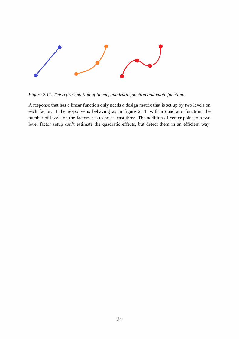
Figure 2.11. The representation of linear, quadratic function and cubic function.
A response that has a linear function only needs a design matrix that is set up by two levels on
each factor. If the response is behaving as in figure 2.11, with a quadratic function, the
number of levels on the factors has to be at least three. The addition of center point to a two
level factor setup can’t estimate the quadratic effects, but detect them in an efficient way.

25
2.5.3 Taguchi Methods
In Japan during the 50s and 60s, Dr. Genichi Taguchi developed techniques for DoE and
implemented several key ideas for experimental design. Taguchi´s parameter design offers an
efficient and systematical approach to optimize design for performance.
The Taguchi designs are similar to the fractional factorial designs, with a standardized set of
orthogonal arrays, but with the implementation of two array matrices for each designed
experiment. The Taguchi design methods are popular when it comes to screening objectives.
(NIST, 2013d)
Taguchi´s design for experiments uses two major tools;
1. Signal to Noise ratio, where control factors and noise factors are separated. The
control factors represent the parameters that can be controlled and varied by the
engineer. Noise factors represent the variation that emerges in for example
manufacturing, and are uncontrolled.
2. The use of orthogonal arrays, which accommodates many design factors
simultaneously. The purpose of the orthogonal array is to investigate as many factors
as possible, with as minimum effort as possible.
A common tool stressed in Taguchi methods is the S/N ratio or, Signal-to-Noise ratio. The
desired values are named signal while undesired values are called noise. The noise factors are
manipulated to create variation, and from the results the control factors can be chosen to
minimize the effect from the generated disturbance, i.e. a more robust design.
There are three categories of the S/N ratio:
1. Nominal the best: 𝑆
𝑁= 10log
ỹ
𝑠𝑦2
In this case a nominal value provides the best characteristics. A specific value is most
desired, and both smaller and larger values are worse.
2. Smaller the better: S/N = −10log1/ƞ(∑𝑦2)
In this case a smaller S/N ratio provides the best characteristics. The ideal value is
zero.
3. Larger the better: S/N = −10log1/ƞ(∑(1 /𝑦2))
In this case a smaller S/N ratio provides the best characteristics. The ideal value is
zero.

26
Table 2.1. Choice of Taguchi “L-designs” dependent on number of factors and levels
The well-known Taguchi orthogonal arrays are the “L´s”. For example, with four factors and
three levels the orthogonal array Taguchi L9 is chosen. See table 2.1 for different
combinations.
Table 2.2. The orthogonal arrays are shown for the yellow, blue and red combinations.
Experiment A B C D
1 1 1 1 1
2 1 2 2 2
3 1 3 3 3
4 2 1 2 3
5 2 2 3 1
6 2 3 1 2
7 3 1 3 2
8 3 2 1 3
9 3 3 2 1

27
2.5.4 Box Behnken
Box Behnken is an efficient design for estimation of first and second order interactions and is
suitable for response surface methodology, invented by Georg E.P Box and Donald Behnken
in the 1960.The setup of a Box Behnken design require some guidelines stated below.
At least three levels are required for Box Behnken, and the factors are leveled as “+1”, “0”
and “-1”. The design appropriate for a quadratic model, as stated, consisting the product of
two factors.
The experiment plan can be considered as a combination of a two level fractional or full
factorial designs, but with an incomplete block design. Each block is designed with a certain
number of factors are varied with all combinations, while the remaining factors are kept at the
nominal value.
Figur 2.13. The Box-Behnken design with spherical design space.
As can be seen in figure 2.13, the design space in Box-Behnken consists of sphere that
protrudes throug the original design space box. Each midpoint of the box is tangential to the
surface of the sphere. This design leads to fewer run than a original center composite design
with the same amount of factors, which makes Box Behnken less expensive. (NIST, 2013e)
Table 2.2 The setup of different Box Behnken designs. Number of factors
Number of factors varied in each block
Number of blocks
Factorial points in each block
Total runs with one center point
Number of coefficients in quadratic model
3 2 3 4 13 10
4 2 6 4 25 15
5 2 10 4 41 21
6 3 6 8 49 28
7 4 7 8 57 36

28
2.5.5 Placket-Burman Design
When interactions between factors are negligible, the idea of Placket-Burman Design is to
find a sequence of experiments where all combinations of levels for any couple of factors or
parameters, are presented the same number of times throughout the experiment plan.
Placket-Burman is very efficient way of screening between a large set of controlled factors,
but only when the main effects are of interest. The reason why Placket-Burman is suitable for
screening is because main factors are, in general, confounded with two factor interactions.
This makes Placket-Burman as a design method very economically for detecting large main
effects, but with the assumptions that interactions are negligible in comparison with the major
main effects. When applying the Placket Burman Design the Pareto principle is present,
which means that the assumption is made that only a few of the factors are considered
contributing with major main effects. This makes Placket Burman the ultimately screening
design, when a few major factors need to be identified. (NIST, 2013f)
Placket- Burmans are so called cyclic designs, where the matrix is generated by one line of
“+” and “-“, with the next line including same sequence, but shifted by one position with the
last line is “+” only.
Figure 2.14. Example of Placket Burman where 11 factors and their main effects are
examined with 12 runs.

29
2.6 Response surface methodology
Response surface methodology is a collection of mathematical and statistical methods that are
used to develop an empirical model of a response. Usually response surface methods are used
when the objective is to optimize a response or to predict the outcome of a certain input
setting of the process. (Mukhopadhyay, 2010).
𝑦 = 𝑓(𝑥1, 𝑥2, 𝑥3, 𝑥4) + ℰ (2.7)
Where y is the response and 𝑥1, 𝑥2, 𝑥3, 𝑥4 are temperatures at different points. ℰ represents the
noise or error in the response. Response functions are usually approximated with a low-order
polynomial with a first order model. A multiple linear approximation model are written as
𝑦 = 𝛽0 + 𝛽1𝑥1 + 𝛽2𝑥2 + 𝛽3𝑥3 + 𝛽4𝑥4 + ℰ (2.8)
The lack of fit of any model can be calculated from statistics or by graphical analysis of the
results. There is often curvature in a response and in those cases a higher degree of
polynomial are applied to the approximation model. A second-order model takes curvature
into account by taking interaction effects between the factors into consideration
𝑦 = 𝛽0 + ∑𝑖=1𝑘 𝛽𝑖𝑥𝑖 + ∑𝑖=1
𝑘 𝛽𝑖𝑖𝑥𝑖2 + ∑∑𝑖<𝑗𝛽𝑖𝑗𝑥𝑖𝑥𝑗 + ℰ (2.9)
For a complete description of the process an even more detailed approximation model can be
used, but this is highly unusual since a response surface of second-degree are often accurate
enough for small regions of the response surface. A full cubic model with all possible terms
can be seen down below
𝑦 = 𝛽0 + ∑𝑖=1𝑘 𝛽𝑖𝑥𝑖 + ∑𝑖=1
𝑘 𝛽𝑖𝑖𝑥𝑖2 + ∑∑𝑖<𝑗𝛽𝑖𝑗𝑥𝑖𝑥𝑗 + ∑∑∑𝑖<𝑗<𝑘𝛽𝑖𝑗𝑘𝑥𝑖𝑥𝑗𝑥𝑘 + ℰ (2.10)
Where 𝛽𝑖𝑗𝑘 are regression coefficients and 𝑥𝑖𝑗𝑘are factor inputs. In order to estimate curvature
in the system a three-level design is needed and in order to get the most efficient results a
proper design matrix with appropriate experimental runs are needed. (NIST, 2013d). Figure
2.15 illustrates how fitted lines change with increasing polynomial order of the approximation
model.
Figure 2.15. Linear-, quadratic- and cubic line fittings.

30
2.6.1 Neural Network Function
Sometimes it is desirable to combine several individual sets of simulation data to create a
response function. A method that makes this possible is the Neural Network Function that
maps numeric input to a set of output targets. The method is feasible when a need of
combining different sets of data, and the data is established for different purposes originally.
MATLAB and ModeFrontier has a Neural Network toolbox which can be used for data
fittings, but also other applications than such as clustering, pattern recognition, dynamic
system modeling and control. In MATLAB, the application assists in selecting data, create the
network and evaluate the performance with mean square error and regression analysis.
A so called two-layer feed-forward network with sigmoid hidden interconnections and linear
output neurons is created. This network can fit multi-dimensional mapping problems given
consistent data and enough neurons in its hidden layer. The network in MATLAB is trained
with a background propagation algorithm, and in ModeFrontier a genetic algorithm is used to
create the neural network response function shown in figure 2.16 (MathWorks, 2014).
Figure 2.16. The two-layer feed forward network used in MATLAB

31
2.7 Regression theory
The approximation models mentioned in previous chapter are often regarded as regression
models. Regression is a statistical method used to estimate the relationship between input
variables and the output response. Regression can be applied in both linear, nonlinear and
multiple manners depending on the amount of input factors. When model assumptions have
been made, the coefficients of the model need to be estimated. The most common method is
the least-square regression model since this method effectively captures factor effects as well
as interaction effects while being insensitive to model error such as coefficient variance.
(Simpson, 2013). The least square regression method seeks to minimize the squared error
calculated from the residuals and the total variance
𝑅2 = 1 − 𝑆𝑟/𝑆𝑡 (2.11)
The 𝑆𝑡 value represents the total variance of the response;
𝑆𝑡 = ∑ (ỹ𝑖
𝑛𝑖=1 − ӯ
𝑖)² (2.12)
where ӯ is the mean value of the response vector. A model with low R2 value does not
guarantee that the model fits the response data well, which also means that the model doesn’t
represent the real process in a satisfying way. Another value often used in close relation to 𝑅2
is the 𝑅𝑎𝑑𝑗2 which is the adjusted value. The 𝑅𝑎𝑑𝑗
2 value increases when significant terms are
added to the model and decreases when they are removed. Thus if insignificant terms are
added to the regression model, the increase of 𝑅𝑎𝑑𝑗2 is small. 𝑅𝑎𝑑𝑗
2 should be close to 𝑅2 to
ensure a good approximation model.
𝑅𝑎𝑑𝑗2 = 1 − (
𝑛−1
𝑛−𝐷𝑂𝐹) (1 − 𝑅2) (2.13)
Where n is the number of experiment and DOF is the degrees of freedom in the
approximation model. The least-square regression method is calculated differently depending
on the approximation model used in the scientific investigation. A linear regression model
seeks to minimize the following
𝑆𝑟 = ∑ (ỹ𝑖
𝑛𝑖=1 − 𝑦𝑖)² = ∑ (ỹ
𝑖𝑛𝑖=1 − 𝛽0 − 𝛽1𝑥1 − 𝛽2𝑥2 − 𝛽3𝑥3 − 𝛽4𝑥4)² (2.14)
Where ỹi is the measured response from the experiment and yi are the response given by the
linear approximation model. Often when there are four independent factors there are
interaction effects between these that contribute to the response. A quadratic model with
interactions instead seeks to minimize
𝑆𝑟 = ∑ (ỹ𝑖
𝑛𝑖=1 − 𝑦𝑖)² = ∑ (ỹ
𝑖𝑛𝑖=1 − 𝛽0 + 𝛽𝑖𝑥𝑖 + 𝛽𝑖𝑖𝑥𝑖
2 + ∑∑𝑖<𝑗𝛽𝑖𝑗𝑥𝑖𝑥𝑗)² (2.15)
The same correlation exists for the cubic approximation model, but will not be mentioned
further here, since higher degree polynomials would result in the danger of over-fitting the
model.
Results of the least-square regression analysis for different approximation models can be seen
in table 4.12. It is theoretically possible to create a model that fits the data exactly. However

32
this will result in a highly oscillating function that cannot be used to predict how the response
is affected by a change in input variables in an effective way (Simpson, 2013).
Determination of test points in matrices depends on the assumed polynomial order of the
assumed mathematical model that is to be used for the response function. The polynomial
order can often be determined from historical testing or by consulting engineers with first-hand knowledge and experience within the area of focus.
2.8 Statistical correlation
Correlation is a statistical technique often used when the purpose is to identify the degree of
relationship between two variables i.e. it tells the degree to which two variables tend to move
together. The correlation coefficient r is calculated by
r =∑(x−x̅)(y−y̅)
nσxσy (2.16)
where n is the sample size i.e. the size of the response vector, x is the factor and the respective
factor mean value, y is the response vector and the respective response mean value. σx, σy is
the square root of the factor and response variance (Benjamin S. Blanchard, 1990)
σx = √∑ x2 − (∑ x)2 (2.17)
σy = √∑ y2 − (∑ y)2 (2.18)

33
2.9 Analysis of variance (ANOVA)
Together with the equations mentioned in section 2.7 and 2.8 it is possible to analyze the
relationship between response and input. This sort of analysis is called an ANOVA analysis.
The purpose of analysis of variance, or ANOVA, is to test the difference between means
when there are several populations in an experiment. It is a statistically based decision tool
that is helpful to derive the significance of all main factors and their respective interactions.
(Rama Rao. S, 2012).
The ANOVA table for a simple linear regression model looks as follows:
Table 2.3. Typical ANOVA table
Source DOF SS MS F P-value
Model k SS(model) MS(model) F(model)
Factor k-1 SS(factor) MS(factor) F(factor)
Error n-k SS(error) MS(error)
Total n-1 SS(total)
The second column in ANOVA tables shows the degrees of freedom for a factor i.e. the
amount of other possible combinations of each factor. Where k is the number of levels used in
the experimental plan and n are the number of experiments. An ANOVA analysis can also be
applied to evaluate a regression model to determine the accuracy of the model. In such cases
the DOF for the complete model is represented by the amount of factors included within the
model. For any regression model with k factors and for any experiment with n observations,
the degree of freedom is calculated as shown in table 2.4.
Table 2.4 Degrees of freedom in ANOVA analysis
Source DOF
Model k
Error n-(k+1)
Total n-1
The SS column shows the sum of squares and is calculated in the same manner as in the least
square regression method presented in eq. (2.12) and (2.13). The total sum of squares become
𝑆𝑆𝑇𝑜𝑡𝑎𝑙 = 𝑆𝑆𝑀𝑜𝑑𝑒𝑙 + 𝑆𝑆𝐸𝑟𝑟𝑜𝑟 (2.19)

34
The third column MS shows the mean sum of squares and is calculated in the same way as the
sum of squares, but divided with the number of experiments and thus shows the mean sum of
squares for the theoretical regression model and for the residuals. (Meier, 2013)
2.9.1 Verification and Validation
The goal of a simulation model is to represent the reality as accurate as possible. Simulation
models have an increasing importance in modern product development, and works as tool for
decisions-making. In especially the aerospace industry, simulation and other computer aided
tools plays a significant role in the development of the product. (Forslund, 2012)
When using the models and the results established from them, is it important that the
information generated is “correct” and really explains the reality in an expected way. The
term validation is here used to express how well the simulation model, and the results based
on it, really represents the reality (Forslund, 2012). In this thesis no validation of the actual
simulation data will be considered, but the awareness must be there when interpreting the
results. Nevertheless, validation in form of statistical methods and tools has to be carried out
on data that are underlying the decisions made through this project.
Verification refers to the evaluation if an internal process complies with specifications or
requirements, in contrast to validation that refers to the assurance that the process meets
stakeholder’s interests.
2.9.2 Fischer F-test
The F-test provides useful statistics that shows the statistical significance of the regression
coefficients. The F-test is a test function for the null hypothesis that shows if there is no linear
relationship between the factors. (Norrby, 2012). The F statistics is calculated in the following
manner
𝐹 =𝑀𝑆𝑚𝑜𝑑𝑒𝑙
𝑀𝑆𝑒𝑟𝑟𝑜𝑟=
𝑆𝑆𝑚𝑜𝑑𝑒𝑙/𝐷𝑂𝐹𝑚𝑜𝑑𝑒𝑙
𝑆𝑆𝑒𝑟𝑟𝑜𝑟/𝐷𝑂𝐹𝑒𝑟𝑟𝑜𝑟 (2.20)
A model or a factor with high F-value that exceeds the critical value will show that there is a
significant effect that is unlikely due to chance. (Winter, 2014). The critical value can be
found in tabulated data when given the DOF values of the numerator and denominator of the
F ratio.
2.9.3 P-Value
The P-value is another method used to evaluate the relationship between factor input and the
response and thereby prove the statistical contribution of each factor. The significance of the
F value is called the P-value and tells the probability of the model statistic being as extreme as
the one observed given that the null hypothesis is true (NIST, 2012a)
𝐻0 : 𝛽1 = 0 (2.21)
The alternative hypothesis is that each of the regression coefficients is different from zero:
H1 : β1 ≠ 0 (2.22)

35
The p-value for which the null hypothesis is rejected is determined by the level of
significance. A common value for the level of significance is α = 5 %, which means that a
p-value lower than 0.05 indicates that the predictor has meaningful effect to the model and
that the null hypothesis, eq. 2.21, can be rejected. (NIST, 2012a)

36
2.10 Selection of Experimental Design
The choice of what experimental plan to use depends on the objective of the experiments, and
the number of factors to be investigated at different levels.
Comparative objective
A comparative objective is if several factors are investigated, but the goal is to make decisions
based on only one priority factor, where the question of interest is whether the factor is
significant or not. The significance of a factor means whether or not a change in the response
is related to different levels of that factor. If this criterion is the main goal of the experiments
that means it is a comparative problem, and therefore needs a comparative design solution.
Screening objective
A screening objective is preferable when the primary purpose is to identify a few important
factors out of many less important ones.
Response Surface objective
Response surface objective is relevant when the experiment design aims at estimate
interaction and even quadratic effects. These designs are suitable when the goal is to find
improved or optimal process settings, finding errors or process problems in weak points and
making a process more robust against external and uncontrollable variation.
Optimal fitting of a regression model objective
When optimal fitting of a regression is the objective, the aim is to model the response as a
mathematical function of a few continuous factors when sufficient model parameters are
desired. This is called a regression design.
Number of
factors
Comparative
objective
Screening
objective
Response
surface
objective
1 One-factor
completely
randomized
design
-
-
2 -4 Randomized
block design
Full or
fractional
factorial
Box
Behnken
5 or more Randomized
block design
Fractional
factorial or
Placket-
Burman
Screen first
to reduce
number of
factors
Figure 2.15. A guideline for selection of experimental design
When it comes to decision making regarding which experimental design to use, there is
several factors to take into account. The extent of the design is a critical factor when limited
resources in terms of time and cost are crucial. The other aspect of this is, what the cost is to
choose the wrong, or more often, a too simple design poor of information. (NIST, 2013g)

37
3. Method
3.1 Literature studies
In order to achieve an understanding of the component and gain required knowledge in the
area of design of experiment, statistics as well as thermal- and structural analysis, literature
studies had to be done. Literature search was done using search engines on the Internet,
Chalmers library and internal documentation search at GKN Aerospace Engine Systems.
Interviews with experts at GKN Aerospace provided valuable information about the
component and the related problems that it was facing.
3.2 Data Acquisition
In order to simulate normal flight conditions data has been collected from temperature
measurements at different positions around the TS. To reduce simulation time the flight cycle
has been reduced to only consider crucial time steps. The flight cycle measurements were
provided by the original engine manufacturer. The data provides a foundation to all
simulation work that was made in this thesis. How this data is used is mentioned further in
chapter 3.5 Thermal analysis.
CAD models were provided by GKN in order to get reliable simulations. The CAD models
were of different composition where some features were width, height and length that had
been altered between the different model configurations. This will be mentioned further in
chapter 3.6 Structural analysis.
3.3 Software research
All simulations were done using ANSYS. The simulation setup for both thermal and
structural analyses as well as post processing of results are presented further in the following
chapters of this thesis. The computer program MATLAB was used for post processing of the
results. MATLAB provided useful functions and the ability to plot the results in a convenient
way. The built-in functions and statistical features of MATLAB 2014a supported fast
evaluation of the data when implementing regression and ANOVA analysis. MINITAB,
ModeFrontier and Microsoft Excel was also used to derive important conclusion from
simulation data and is useful software when working with design of experiments.

38
3.4 Development process
The team working with the development of the TS at GKN Aerospace is a multidisciplinary
team of engineers with different expertise and responsibilities. In order to improve concepts
and gain a higher level of technological readiness the team works in a highly iterative manner
in order to test and evaluate different concepts. The concepts have a highly demanding
specification that needs to be met in order to meet the high certification requirements put on
commercial jet engines. EWB evaluates a set of design definitions by performing analyses
and post processing the results. Data from all simulations are gathered to be examined and
evaluated. The product development process of the multidisciplinary team can be seen in
appendix I, only for the internal report, and shows what input and output each process has.
The process chart has a strong focus on thermal analysis since the goal of this thesis is to
increase the thermal robustness of the component.
The development chart is based on interviews with several of GKN employees working in the
EWB start platform. A start platform is created based on findings from earlier designs and a
system model of the jet engine. Altogether this becomes a design study. In the next stage the
team decides what they want to analyze. A hypothesis is created and several different
geometries are tested in an iterative manner. In the next step a mesh is created and provided as
input for the thermal analysis, the structural analysis as well as for stiffness- and weld
analysis. Subsequent processes run parallel with each other and all the results are collected in
a final database which shows trend curves or response surfaces that are used for providing
reliable feedback for the specific design case. A so called CUMFAT analysis is performed
subsequently of the structural analysis in order to determine the component life. The OEM
performance group is the abbreviation for the informative data input given by the original
engine manufacturer. A large effort of the process chart was put on the generation of thermal
input that is provided for the thermal analysis and this will be further described in the
following section.

39
3.5 Thermal analysis
As seen in appendix II the process chart contains the all through process of generating the
thermal input. OEM provides data from any given flight cycle supported with measured
temperatures at several points in the jet engine. This is compiled to a complete LCF mission
showing engine parameters versus time for the given flight mission.
Calculations of airflow, heat transfer coefficients and heat are needed to apply appropriate
thermal loads. This is implemented by several computer macros that eventually provide
ANSYS input tables with interpolated temperature that are applied on all the surfaces of the
CAD model. The flight cycle provided by OEM is divided into a certain amount of time steps
that are chosen by experience. Many time steps require long simulation time or high computer
power, but in the contrary fewer time steps require shorter simulation time and provide
possibilities for multiple simulations at the same time.
3.6 Structural analysis
The structural analysis is performed subsequently to the thermal analysis since it requires a
thermal result file as input. The thermal result file is applied on the model and the model is
locked in its six DOF. ANSYS is also used for this analysis and it calculates elongation and
stress levels emerging from thermal expansion at all nodes in the whole model. The result
files consist of this information and are used for subsequent post processing of the results.

40
3.7 Post processing of simulation data and use of statistical methods
Evaluation of simulation and DoE data should be performed systematically and in iterative
fashion. This section describes how post processing operation is performed for evaluation of
DoE data given from structural and thermal analysis. The overall process that was used is
presented in figure 3.1 and shows the DoE analysis flowchart. The process follows a
methodology presented by NIST Handbook of Statistical Methods (NIST, 2012b)
3.8 Geometrical variation
To investigate the geometrical variation based on data from older models a neural network
function was generated in MATLAB. With aid from a neural network function the data set of
varied geometrical models together with the thermal results were mapped as numeric input to
a set of output targets. The results derived from the neural network were used for
investigation of geometrical and thermal factors.
Figure 3.1. DOE analysis flowchart

41
4. Results
This chapter presents the derived results from the thesis work.This chapter also describes how the theory and methodologies earlier presented was implemented in the ongoing thesis
work.
4.1 Selection of process parameters
An initial research was started to fully understand the presented thermal problem. To gain this
knowledge a research study in literature and utilization of internal information was conducted.
A mapping of the product development process was made as mentioned in section 3.4. The
mapping helped to understand what matters that were actually needed to address. The
investigation supported the creation of the research question of this thesis report. Following
the procedure of DOE related work mentioned in chapter 2.5, a cause and effect analysis was
performed in order to establish the important process parameters to be included in the
analysis. A fishbone diagram, shown in figure 4.1 was used to gain an understanding of the
underlying causes of stress in the TS. As it can be seen the diagram spreads into four main
sectors.
Figure 4.1 Fishbone diagram showing root causes of stress.
Geometric attributes
This sector covers all the geometrical variables that change the topology and positioning of all
the parts in the TS.

42
Loads
This sector covers both the outer forces that act on the TS and the thermal loads emerging
from the hot gasses exiting the low pressure turbine. No consideration to mechanical loads
was taken during this analysis. The analysis focused on investigating how thermal boundary
conditions (Thermal loads) affected stress distributions in the TS.
Material
This section regards the material parameters used for the analysis. There are the Young’s
modulus, Poisons ratio and the alpha value, for all of which was not investigated during this
thesis work.
Model uncertainties
Model uncertainties originate from what constraints that was used when building the model. It
also covers the definition of loads and how these are applied to the simulation model and at
last there are model uncertainties emerging from the use of different mesh sizes and shell
models.
4.2 Thermal Management
As presented in chapter 2.2, the TS is a rotational symmetric component and consists of 14
struts, 11 regular and 3 mount struts, see figure 2.3. When studying the TS it early stood clear
that the area of focus had to be reduced in order to grasp the problem in an efficient way. It
has been mentioned that GKN experienced shortened life and crack initiation at weld
positions. It was therefore decided that the area of research should concern welds around strut
sections of the TS. The load bearing mount struts are especially important for this study,
where the most stress sensitive area should be investigated. Therefore the examined strut is
one of the load bearing mount struts shown in figure 4.2
Figure 4.2 Mount strut position on the TS

43
One of the major concerns when it comes to simulation is the limitations in time and
processing capacity, which demands an efficient set up of the model. The thermal zones
surrounding the TS were divided into four zones. The main zones are the gas canal, the
secondary airflow (bleed air), the nacelle and the hub cavity. The arrangement of the thermal
zones can be seen in figure 4.3.
Figure 4.3. The figure shows a side view cross section of the TS and illustrates a side view of
one of the 14 struts.
As seen in the figure different temperatures act on each surface of the TS cross section. The
nacelle is a cavity outside the case of the TS and the secondary airflow are a cavity of air
emerging within the core of the jet engine. In this report the mentioned temperatures will be
named as thermal boundary conditions or thermal BC’s. Temperature measurements for each
surface were provided by GKN and as mentioned earlier they are measurements from a real
flight cycle. Thermal BC’s were interpolated between measurement points and was provided
as ANSYS input tables for thermal analysis as described in chapter 3.5 Thermal analysis.

44
4.3 Experimental plan
The TS is now sectional divided into a segment including one bearing mount strut, see figure 4.3. The selected four thermal zones shown in figure 4.2 could now be used as four different input factors for the upcoming experimental study. To investigate each zones effect and contribution to the resulting stresses in the TS, a design of experiment plan was set up. As an initial study and for the purpose of investigating the thermal robustness of the TS, consideration was only taken to the thermal loads. The division of the TS into four thermal zones now served as four factors for a DoE design. The initial set up was a screening design, where the goal was to identify the main effects (i.e. the effect each factor has on the output response) of the chosen factors. The initial idea was to test the factors at three levels, to be able to identify a quadratic response. This together with four factors generates a Taguchi L9 design, according to table 2.1. The experimental setup is presented in figure 4.5.
Experiment Run A B C D
1 -1 -1 -1 -1
2 -1 0 0 0
3 -1 1 1 1
4 0 -1 0 1
5 0 0 1 -1
6 0 1 -1 0
7 1 -1 3 0
8 1 0 -1 1
9 1 1 0 -1
Figure 4.5. The design set up for Taguchi L9
An early assumption for the thermal variation in the experimental plan was 28K. Literature
studies suggest that this temperature level should be
∆𝑇 = µ + 3𝜎 (4.1)
Where µ is the mean temperature value of all the measurements and 𝜎 is the standard
deviation of all measurements (Vilmart, 2010)
Temperatures are varied between -1, 0 and +1. The assumption was made that the temperature difference established represented a realistic variation in the input parameters from OEM .The complete Taguchi L9 temperature table contains data measurements from a real flight cycle, but will not be shown here for confidential reasons. The data collected from a real flight cycle consists of over 400 time steps distributed from engine start until engine shut down. To minimize simulation time the original data were interpolated and narrowed down to 41 representative time steps.
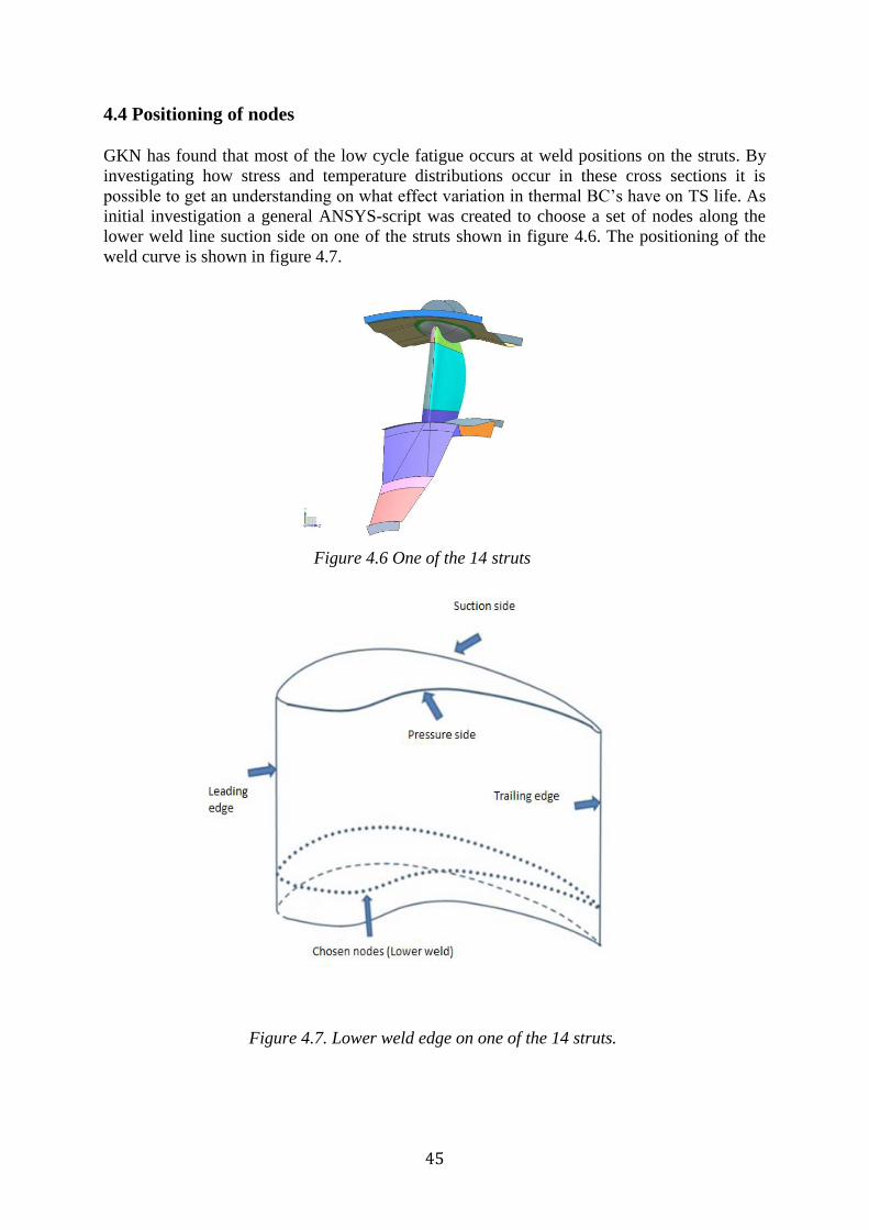
45
4.4 Positioning of nodes
GKN has found that most of the low cycle fatigue occurs at weld positions on the struts. By
investigating how stress and temperature distributions occur in these cross sections it is
possible to get an understanding on what effect variation in thermal BC’s have on TS life. As
initial investigation a general ANSYS-script was created to choose a set of nodes along the
lower weld line suction side on one of the struts shown in figure 4.6. The positioning of the
weld curve is shown in figure 4.7.
Figure 4.6 One of the 14 struts
Figure 4.7. Lower weld edge on one of the 14 struts.
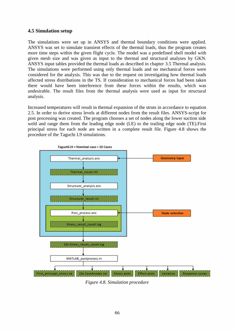
46
4.5 Simulation setup
The simulations were set up in ANSYS and thermal boundary conditions were applied.
ANSYS was set to simulate transient effects of the thermal loads, thus the program creates
more time steps within the given flight cycle. The model was a predefined shell model with
given mesh size and was given as input to the thermal and structural analyses by GKN.
ANSYS input tables provided the thermal loads as described in chapter 3.5 Thermal analysis.
The simulations were performed using only thermal loads and no mechanical forces were
considered for the analysis. This was due to the request on investigating how thermal loads
affected stress distributions in the TS. If consideration to mechanical forces had been taken
there would have been interference from these forces within the results, which was
undesirable. The result files from the thermal analysis were used as input for structural
analysis.
Increased temperatures will result in thermal expansion of the struts in accordance to equation
2.5. In order to derive stress levels at different nodes from the result files. ANSYS-script for
post processing was created. The program chooses a set of nodes along the lower suction side
weld and range them from the leading edge node (LE) to the trailing edge node (TE).First
principal stress for each node are written in a complete result file. Figure 4.8 shows the
procedure of the Taguchi L9 simulations.
Figure 4.8. Simulation procedure

47
As it can be seen in figure 4.8 the post process script generates result files for each load case
simulation performed in order of the Taguchi L9 table presented in chapter 4.3. All results
files were then compiled using MATLAB in the MATLAB post process program file. This
program was also used to generate response curves, plots of the results, effect plots and to
calculate related statistics. To this purpose MINITAB and Excel were also used which will be
described later in this report.

48
4.6 Temperature and stress distributions
This section will describe the findings from the thermal and structural analyses performed in
ANSYS.
4.6.1 Thermal distribution
When performing a thermal analysis on the nominal model some interesting observations
could be seen. When the TS is exposed to hot gasses from the jet stream exiting the LPT, the
struts rapidly begin to heat and expand in contrary to the outer shell and the hub that is still
cold. Temperature also reaches its highest levels in stages of take-off and there are clear signs
of cyclic temperature levels between idle phase and take-off. Figure 4.11 in the following
section shows how this affect stress in one of the struts.
4.6.2 Stress distributions
In the initial stage a structural analysis was performed in order to get a better understanding of
what processes that are taking place during the flight cycle. An example from the structural
analysis is shown in figure 4.9 and shows stress distributions in the TS for one time step and
for one of the thermal load cases. When the structure is heated the hub tends to rotate due to
the thermal expansion taking place in all struts as can be seen in figure 4.9 below. The
thermal expansion in the figure is heavily enhanced to show a tendency that eventually leads
to buckling of the TS.
Figure 4.9 Skewed Turbine Structure.
ANSYS result files provided stress measurements for all direction as well as von Mises
stresses in all nodes. Von Mises stresses provides a value without direction and is therefore
not as important for crack initiation. First principal stress was chosen due to the fact that it has
a direction and is always pointing in the direction of which the stress has the highest levels. It
is therefore a favorable quantity to observe when evaluating risk for crack initiation.

49
4.7 Analysis of the results
Reflecting back on the basic procedure of DOE analysis presented in chapter 2.5 and
especially analysis and interpretation of the results, several steps was used in order to examine
the data.
The first steps of the result analysis were simply visual examination of the data. Scatter plots
was used to interpret any linearity in the response vector. Surface plots were used to identify
what section of the weld edge that had the highest stress levels during the whole flight cycle.
Figure 4.10 shows a surface plot of one of the 10 thermal load cases that was applied to the
model. The Taguchi L9 experimental plan only consist of 9 runs, but an additional nominal
load case with only zeroes was also included in the experimental plan. The X- and Y-axis
shows node numbers along the suction side weld on the TS and flight cycle ranging from
take-off to landing of the airplane. As it can be seen there are valleys with low stress
amplitudes in the middle of weld edge. The highest stress amplitudes occur in the beginning
of the flight cycle and can be found close to the leading edge or close to the trailing edge of
the vane. This supports that in future post processing operations it is beneficial to only study
the nodes furthest to the leading edge and to the trailing edge of the strut.
Figure 4.10. First principal stress on suction side weld vs. flight cycle

50
4.8 Scatter plots
Scatter plots were created using MATLAB and was used to derive conclusion regarding linear
relationships between the response and the zone temperatures. The scatter plot in figure 4.11
shows that temperature differences in zones are related to a response, but the linearity is
somewhat unclear. There are some tendencies that show a stress front for temperature
increase in zone 2. Temperatures in zone 1 and 4 are clustered in the same way and shows
that these zones share some relationship. In zone 3 it can be seen that there is a tendency to a
non-linear relationship between zone 3 temperatures and the stress in the LE node. Zone1, 3
and 4 shows that there’s an outlier clusters of stress measurements in all of these plots. In
overall there was proof that variation in stress amplitudes depended on temperature levels, but
there was still unknown what the underlying causes of variation were.
Figure 4.11. Scatter plots showing stress as a function of temperature in the different thermal zones.

51
4.9 Normal probability plot
A normal probability plot was used in order to assess if data was normally distributed. The
plot of the standard deviations of our response in figure 4.12 showed that there was a spread
in data at stresses over the 0.06 normalized stress level and that there was undesirable noise
within the process. There are high fluctuations in stress levels over the whole flight cycle and
the normal probability plot indicates that there are departures from the normality condition. A
conclusion that can be drawn from the plot is that normal distribution is not a good model for
these data measurements since there are nonlinear patterns in the results.
Figure 4.12 Normal probability plot

52
4.10 Temperature gradient plots
When having analyzed the data to this point it stood clear that it had to be some underlying
process that caused variation in the response. A hypothesis was that there could in fact be
linear relationships in temperature gradients. The key issue was then to identify temperature
gradients that drive stress increase in the weld. Temperature gradients were calculated using
MATLAB and plotted against stress levels in LE node. The result of this procedure can be
seen in figure 4.13. Temperature gradient between zone 1 and zone 2 shows some linear
relationships or a cluster of points emerging after a specific increase in delta T. Temperature
gradients between zone 1 and zone 2, zone 1 and zone 3, zone1 and zone 4 as well as zone 3
and zone 4 show no sign of linear relationship. Temperature gradients between zone 2 and
zone 3 shows a linear relationship with increasing stress levels in relation to temperature, but
there are still clustered outliers departing from the rest of the results. A nonlinear relationship
can be seen for temperature gradients between zone 2 and zone 4.
Conclusions that could be drawn from these results were that there was no clear evidence of
specific temperature gradients causing stress increase in LE node. There is also a large
variation in the response which indicates that there are other factors causing stress increase in
the node. At this point another hypothesis was that there are transient effects within the flight
cycle causing “lag” in the stress amplitudes. There is a transient effect between air
temperature and actual stress increase emerging from thermal expansion in the TS. It was
Figure 4.13. Temperature gradients between thermal zones.

53
therefore decided to analyze steady state points within the flight cycle that have a fully
developed flow and the transient effects have been overcome.
To account for transient effects occurring along the flight cycle, MATLAB was used to
reduce the flight cycle to study steady state points. Figure 4.14 shows temperature gradient
plots for reduced flight cycle and doesn’t show any signs of linearity. The data points are
randomly distributed within the intervals of temperature difference. It is therefore difficult to
develop any kind of model that fits to these data points.
Figure 4.14. Temperature gradients between thermal zones for reduced flight cycle

54
4.11 Main effects plots
To gain a further in depth understanding of the data a main effect plot was created in
MINITAB in order to identify the most important factor in the experiment. The main effect
function calculates the shift in average response as the experiment moves from minus to plus
in the experimental plan. The factor with the largest shift is the most important factor and the
one with the least are the least important. (NIST, 2012c). The main effects from the different
thermal zones are shown in figure 4.15. As it can be seen zone 1 and zone 2 has the most
important effect to stress increase when increasing temperature. Zone 4 has the largest
negative effect thus an increase in temperature in this zone causes decreasing stress levels.
The factor with the least important effect is zone 3 which also has a negative effect on stress
amplitudes in the LE node.
Figure 4.15. Main effect plots corresponding LE for the different thermal zones
In close relation to the main effect plot there is the interaction plot which shows the effect of
interactions between each thermal zone as the experimental plan moves from minus one to
plus one. The interaction plot includes both interaction effects between two factors as well as
main effects. Figure 4.16 shows how mean stress levels change depending on the interaction
between the thermal zones. Interactions with steep lines show that the factor is more
important than for factors with flat lines. The interaction plot provided good understanding on
how the thermal zones interact as the temperature levels change. For example it can be seen
that for an interaction between zone 1 and zone 2 (T1 & T2), an increase in temperature in the
gas canal (T2) will increase the stress in LE node if keeping the nacelle temperature at
nominal temperature or at a 28K increase. On the other hand the stress will decrease if the
nacelle temperature is lowered. The interaction plots may seem easy to interpret but
confounding between factors and interactions needs to be taken into consideration in order to
avoid deceptive information regarding the process.

55
Figure 4.16. Interaction plot corresponding LE for the different thermal zones
After having investigated the LE node it was of interest to evaluate if the same relationship
could be seen for the trailing edge node. A main effect plot considering the stress at the TE
node shows a significant effect for the zones T2 and T4, as seen in figure 4.17. T2 has a
positive influence on the response and T4 has similar effect but negative. The effects of T1
and T3 are now less significant. A specific defined limit for what is considered a contributing
effect is represented as the P-value described in chapter 4.14.1.
Figure 4.17. Main effect plots corresponding LE for the different thermal zones

56
The interaction plot shows how a temperature difference in any of the thermal zones affect the
mean stress values derived from the TE node. For example, It can be seen in figure 4.18 that
the stress are decreasing when T2 is held constant for all levels, when T4 the temperature in
zone 4 are increased.
Figure 4.18. Interaction plot corresponding TE for the different thermal zones
By help of these graphs it is easier to interpret how a specific temperature gradient will
change stress levels in the TS. By only looking at the temperature gradient plots it is difficult
to understand that the stress levels in each plot are a combined result emerging from
temperature gradients between all zones. Distinguishing the power of certain temperature
gradients are therefore easier by help of interaction plots.
4.12 Effect of thermal zones
In order to get a greater understanding of how the main effects (eq. 2.6) change during the
whole flight cycle, effect plots were created using MATLAB. The effect of all thermal zones
was calculated for all previously mentioned nodes, load cases and for the whole flight cycle
according to the method described in chapter 3. Figure 4.19 shows how the effect varies at
node 1 along the suction side weld of the mount strut during the whole flight cycle. Referring
to the different zones mentioned in section 4.1, Zone 1 and Zone 2 has large positive impact
on first principal stress in node 1. Zone 3 and 4 on the other hand provides a large negative
effect. The effect curves for this geometry have been calculated for all nodes on the suction
side weld. In a later stage it will be possible to analyze any predefined weld or edge that is of
interest for the analysist.

57
Figure 4.19. Main Effect levels at the LE node.

58
4.13 Correlation
The correlation coefficients between the thermal zones and the stress in the leading edge node
were calculated in MINITAB using eq. 2.15. Table 4.1 shows the correlation coefficient for
the different zones. The correlation coefficient only tells to what range two variables tend to
move together and thus it can be seen that there is a strong correlation for increasing stress
when increasing the temperature in the gas canal. The least correlation exists between stress
and temperature levels in the bleed air cavity of zone 3.
Table 4.1. Correlation table
Correlation: T1; T2; T3; T4; Stress
T1 T2 T3 T4
T2 0,709
T3 0,866 0,614
T4 0,921 0,715 0,851
Stress 0,385 0,618 0,078 0,249
4.14 Response surface methodology
When having evaluated the data without seeing any clear relationship the next step was to
develop a theoretical model of the data. This section will regard the creation of a theoretical
model that is evaluated through statistical tools in order to create a response function that
matches simulation results. The theoretical models were used to create response surfaces that
could be used for optimization and interpretation of stress amplitudes under certain load
conditions.
The built in statistical toolbox package of the mathematical software MATLAB was used do
derive the coefficients of the approximation models and especially to derive response surface
fits. The functions fitlm and anova were used to in a fast and effective way evaluate different
approximation models, by providing the useful statistics mentioned in chapter 2.12. The
regression models that were evaluated were linear, interaction, quadratic and a pure quadratic
model. The multiple linear regression models are given by eq. (2.7) through (2.10).

59
4.14.1 Analysis of Variance
An analysis of variance was conducted in order to interpret what thermal zones that gave the
largest statistical effect over the whole experiment. The ANOVA analysis uses statistical
calculations presented in chapter 2.9. Results from the analysis derived from the LE node are
shown in the table 4.2.
Table 4.2 SumSq DF MeanSq F pValue
__________ ___ __________ ______ _________
x1 1.6874e+16 1 1.6874e+16 7.2969 0.0071976
x2 1.4406e+16 1 1.4406e+16 6.2294 0.012961
x3 1.0586e+16 1 1.0586e+16 4.5777 0.032987
x4 2.0609e+16 1 2.0609e+16 8.9115 0.0030056
Error 9.3659e+17 405 2.3126e+15
From these results it could be derived that zone 3 has the least significant effect on the stress
in the LE node. Most significant is zone 4, the hub cavity.
The analysis was also performed on the trailing edge node shown below in table 4.3
Table 4.3 SumSq DF MeanSq F pValue
__________ ___ __________ __________ __________
x1 4.1862e+12 1 4.1862e+12 0.00097499 0.97511
x2 5.788e+16 1 5.788e+16 13.48 0.00027335
x3 4.0686e+14 1 4.0686e+14 0.09476 0.75837
x4 5.1452e+16 1 5.1452e+16 11.983 0.00059388
Error 1.7389e+18 405 4.2936e+15
The results showed that the significance of zone 2 and zone 4 had increased while
significance of zone 1 and zone 3 had reduced. The analysis showed that zone 2 (gas canal)
had the greatest effect on stress in all nodes along the weld edge. Significance of zone 1
(nacelle) and zone 3 (bleed air cavity) tends to reduce when analysing nodes closer to the
trailing edge.

60
4.14.2 Linear model
A linear regression model was first evaluated for fit against the simulation data. The model
was written as according to eq. 2.8 and was calculated for the LE node. The ANOVA analysis
showed the following relationship.
Table 4.4 SumSq DF MeanSq F pValue
__________ ___ __________ ______ __________
x1 1.8804e+17 1 1.8804e+17 268.4 1.2023e-46
x2 2.8796e+17 1 2.8796e+17 411.04 1.3627e-63
x3 1.7298e+17 1 1.7298e+17 246.9 8.8005e-44
x4 6.8319e+16 1 6.8319e+16 97.518 9.466e-21
Error 2.8373e+17 405 7.0058e+14
MATLAB function regstats calculated R2, Adjusted R2 , F-statistics and P-value and these are
shown in the table 4.12 . The ANOVA analysis, table 4.4 showed that for a linear regression
model all terms become significant and should therefore be included in the model.
The linear model and instead using the TE node as response vector will show the following
relationship.
Table 4.5 SumSq DF MeanSq F pValue
__________ ___ __________ ______ __________
x1 1.487e+17 1 1.487e+17 108.54 1.1227e-22
x2 5.3009e+17 1 5.3009e+17 386.91 6.0228e-61
x3 1.2375e+17 1 1.2375e+17 90.323 1.8094e-19
x4 3.2522e+16 1 3.2522e+16 23.737 1.5871e-06
Error 5.5487e+17 405 1.3701e+15
As same as before it could be seen from table 4.5 that all terms in the model were significant.
MATLAB function regstats calculated R2, Adjusted R2 , F-statistics and P-value and these are
shown in the table 4.12 in the same manner as before.

61
4.14.3 Interaction model
An interaction model according to eq. 4.2 for LE node will produce the following ANOVA
table.
𝑦 = 𝛽0 + ∑𝑖=1𝑘 𝛽𝑖𝑥𝑖 + ∑∑𝑖<𝑗𝛽𝑖𝑗𝑥𝑖𝑥𝑗 + ℰ (4.2)
Table 4.6 SumSq DF MeanSq F pValue
__________ ___ __________ ______ __________
x1 8.6449e+16 1 8.6449e+16 206.24 5.397e-38
x2 2.357e+17 1 2.357e+17 562.32 3.3801e-78
x3 9.1351e+16 1 9.1351e+16 217.94 1.1654e-39
x4 5.0756e+16 1 5.0756e+16 121.09 8.9297e-25
x1:x2 1.5078e+16 1 1.5078e+16 35.973 4.4884e-09
x1:x3 6.0501e+15 1 6.0501e+15 14.434 0.00016782
x1:x4 1.1204e+15 1 1.1204e+15 2.673 0.10285
x2:x3 1.5676e+16 1 1.5676e+16 37.398 2.2977e-09
x2:x4 1.8287e+16 1 1.8287e+16 43.627 1.2717e-10
x3:x4 2.0423e+15 1 2.0423e+15 4.8724 0.027859
Error 1.6725e+17 399 4.1916e+14
MATLAB function regstats calculated R2, Adjusted R2 , F-statistics and P-value was
calculated in the same way as before and these are shown in table 4.12. The ANOVA analysis
for this model shows that the interaction term between zone 1 and zone 4 is greater than the 5
% significance level and it could therefore be neglected for further evaluation if the model
was to be chosen at a later stage.
For the TE node the following relationship is present.
Table 4.7 SumSq DF MeanSq F pValue
__________ ___ __________ ______ __________
x1 3.6702e+16 1 3.6702e+16 50.656 5.1475e-12
x2 4.7152e+17 1 4.7152e+17 650.79 7.7372e-86
x3 2.8025e+16 1 2.8025e+16 38.68 1.2615e-09
x4 5.701e+16 1 5.701e+16 78.684 2.4713e-17
x1:x2 2.011e+16 1 2.011e+16 27.756 2.2565e-07
x1:x3 1.4148e+15 1 1.4148e+15 1.9527 0.16307
x1:x4 6.5401e+15 1 6.5401e+15 9.0266 0.0028287
x2:x3 2.6212e+16 1 2.6212e+16 36.178 4.0756e-09
x2:x4 1.4411e+16 1 1.4411e+16 19.889 1.0683e-05
x3:x4 5.7552e+15 1 5.7552e+15 7.9432 0.0050671
Error 2.8909e+17 399 7.2454e+14
MATLAB function regstats calculated R2, Adjusted R2 , F-statistics and P-value was
calculated in the same way as before and these are shown in table 4.12. Table 4.7 show that
relationships are switched when evaluating the trailing edge node. The interaction term
between zone 1 and zone 3 becomes insignificant and could therefore be neglected at a later
stage.

62
4.14.4 Purequadratic model
A purequadratic regression model was also chosen for evaluation. The model is the same
equation 2.9 but without interaction terms, and thus only include the quadratic terms. The
ANOVA analysis, table 4.8, shows the following relationship for the different thermal zones
and stress in the LE node.
Table 4.8 SumSq DF MeanSq F pValue
____________ ___ ___________ _________ _________
x1 1.18093e+17 1 1.18093e+17 232.229 1.08027e-41
x2 2.19456e+17 1 2.19456e+17 431.559 1.34588e-65
x3 9.88822e+16 1 9.88822e+16 194.451 2.59821e-36
x4 3.94765e+16 1 3.94765e+16 77.630 3.80246e-17
x1^2 1.94543e+16 1 1.94543e+16 38.256 1.53051e-09
x2^2 5.33518e+16 1 5.33518e+16 104.916 5.01636e-22
x3^2 8.86640e+15 1 8.86640e+15 17.435 3.64828e-05
x4^2 1.03436e+16 1 1.03436e+16 20.340 8.52217e-06
Error 2.03916e+17 401 508519187481845
MATLAB function regstats calculated R2, Adjusted R2 , F-statistics and P-value was
calculated in the same way as before and these are shown in the table 4.12. All the terms in
this model proved to be significant since all terms are below the 5% threshold.
The analysis of the TE node showed the following relationship.
Table 4.9 SumSq DF MeanSq F pValue
__________ ___ __________ ______ __________
x1 6.5722e+16 1 6.5722e+16 72.727 3.0785e-16
x2 4.4541e+17 1 4.4541e+17 492.88 8.4648e-72
x3 3.4044e+16 1 3.4044e+16 37.672 2.0126e-09
x4 4.0305e+16 1 4.0305e+16 44.6 8.0836e-11
x1^2 8.4603e+15 1 8.4603e+15 9.3619 0.0023642
x2^2 1.5098e+17 1 1.5098e+17 167.07 3.436e-32
x3^2 2.8105e+15 1 2.8105e+15 3.11 0.078573
x4^2 5.0251e+16 1 5.0251e+16 55.607 5.5222e-13
Error 3.6238e+17 401 9.0369e+14
MATLAB function regstats calculated R2, Adjusted R2 , F-statistics and P-value was
calculated in the same way as before and these are shown in table 4.12 for later evaluation.
The ANOVA analysis, table 4.12, shows that the quadratic term of zone 3 is insignificant and
could therefore be neglected at a later stage.

63
4.14.5 Quadratic model
A quadratic regression model was also implemented in accordance to eq. 2.9. The analysis
shows that all the interaction has significant effect since the p-value is less than the
significance level of 5 %.
Table 4.10 SumSq DF MeanSq F pValue
__________ ___ __________ _______ __________
x1 9.2496e+16 1 9.2496e+16 241.59 7.5398e-43
x2 2.2838e+17 1 2.2838e+17 596.5 5.9254e-81
x3 9.2333e+16 1 9.2333e+16 241.17 8.606e-43
x4 4.8265e+16 1 4.8265e+16 126.07 1.4118e-25
x1:x2 4.2532e+15 1 4.2532e+15 11.109 0.00094021
x1:x3 2.4873e+15 1 2.4873e+15 6.4967 0.011185
x1:x4 2.7738e+14 1 2.7738e+14 0.72449 0.39519
x2:x3 1.0561e+16 1 1.0561e+16 27.584 2.4642e-07
x2:x4 1.2227e+15 1 1.2227e+15 3.1936 0.074694
x3:x4 4.9735e+15 1 4.9735e+15 12.99 0.00035311
x1^2 1.9939e+14 1 1.9939e+14 0.5208 0.47093
x2^2 2.6226e+14 1 2.6226e+14 0.68501 0.40837
x3^2 8.6875e+15 1 8.6875e+15 22.691 2.6766e-06
x4^2 6.3212e+15 1 6.3212e+15 16.511 5.8383e-05
Error 1.5123e+17 395 3.8286e+14
MATLAB function regstats calculated R2, Adjusted R2 , F-statistics and P-value was
calculated in the same way as before and these are shown in table 4.12. The ANOVA table
shows terms with underlined insignificant values. These could be neglected at a later stage
when full model evaluation has been made.
For the TE node the ANOVA table for the quadratic model looks as following.
Table 4.11 SumSq DF MeanSq F pValue
__________ ___ __________ _______ __________
x1 4.0925e+16 1 4.0925e+16 59.11 1.196e-13
x2 4.4178e+17 1 4.4178e+17 638.09 1.7487e-84
x3 3.1812e+16 1 3.1812e+16 45.947 4.4364e-11
x4 5.4737e+16 1 5.4737e+16 79.06 2.1768e-17
x1:x2 5.4058e+15 1 5.4058e+15 7.8079 0.0054553
x1:x3 3.1301e+15 1 3.1301e+15 4.521 0.0341
x1:x4 1.1036e+15 1 1.1036e+15 1.594 0.2075
x2:x3 1.8752e+16 1 1.8752e+16 27.085 3.1369e-07
x2:x4 1.6204e+14 1 1.6204e+14 0.23404 0.62881
x3:x4 2.8604e+15 1 2.8604e+15 4.1314 0.042762
x1^2 1.6139e+15 1 1.6139e+15 2.331 0.12762
x2^2 7.1464e+14 1 7.1464e+14 1.0322 0.31027
x3^2 3.8911e+15 1 3.8911e+15 5.6201 0.018235
x4^2 6.3408e+15 1 6.3408e+15 9.1584 0.0026379
Error 2.7348e+17 395 6.9235e+14
MATLAB function regstats calculated R2, Adjusted R2 , F-statistics and P-value was
calculated in the same way as before and these are shown in table 4.12. The ANOVA

64
analysis, table 4.11, shows terms with underlined insignificant values. These could be
neglected at a later stage when full model evaluation has been made. The interaction term
between zone 1 and zone 4, zone 2 and zone 4, squared term of zone 1 and zone 2 all proved
to be insignificant.
Table 4.12
Summary R-square Adjusted R-square F-statistics P-value
Linear model (LE) 0.716000212648254 0.713195276476879 2.5526e+02 2.8921e-109
Linear model (TE) 0.699850211128788 0.696885768769566 2.3608e+02 2.0674e-104
Interaction model (LE) 0.832596603228597 0.828401029374677 1.9844e+02 4.6304e-148
Interaction model (TE) 0.843620359329262 0.839701070089394 2.1524e+02 6.1138e-154
Purequadratic model (LE) 0.795892838160611 0.791820874832144 1.9545e+02 2.9643e-133
Purequadratic model (TE) 0.803977001184381 0.800066317916240 2.0558e+02 9.2465e-137
Quadratic model (LE) 0.848629044854405 0.843263998342916 1.5817e+02 3.9337e-152
Quadratic model (TE) 0.852065989304816 0.846822758546000 1.6251e+02 4.3182e-154
The regression models show that we have the least fit in a linear model and the best fit in a
quadratic model with 𝑅2 = 0.8521 as seen in table 4.12. The ANOVA table also shows that
there are some insignificant factors that can be discarded from the model since they show a
probability greater than the 5% significance level. An interaction factor between zone 1 and
zone 4, between zone 2 and zone 4, as well as quadratic factors of zone 1 and zone 2, can be
discarded since the p-value is greater than 0,05. Before reducing the model it was important to
know if the residuals are normally distributed around zero.
It was seen in table 4.11 that some terms in the model could be neglected due to their
insignificance. The reduced LE node model then became
𝑦 = 𝛽0 + ∑𝑖=1𝑘 𝛽𝑖𝑥𝑖 + 𝛽5𝑥1𝑥2 + 𝛽6𝑥1𝑥3 + 𝛽7𝑥2𝑥3 + 𝛽8𝑥3𝑥4 + 𝛽9𝑥3
2 + 𝛽10𝑥42
The reduced model for the TE node was also the same since same terms was reduced from the
model. A new ANOVA analysis was conducted which showed that the terms for zone 1 and
zone 4, as well as interaction term for zone 1 and zone 3 were insignificant for the model and
thus could be neglected.
Table 4.13
Summary R-square Adjusted R-square F-statistics P-value
1st reduced model(LE) 0.8395 0.8354 208.6213 1.1425e-151
1st reduced model(TE) 0.8491 0.8454 224.5952 4.7907e-157
2nd reduced model(LE) 0.8368 0.8346 344.9113 2.5905e-155
2nd reduced model(TE) 0.8408 0.8389 421.8732 7.2820e-158
The results from these analyses, table 4.13, revealed that reduced models did produce better
F-values with greater significance. The critical F-value for a model of 6 terms and 410
observations was found in tabulated data for a 5 % significance level giving
𝐹(0.05,5,405) = 2.236. The F-value for the second reduced model of both LE and TE node are
much larger than the critical value thus the null hypothesis can be rejected. A lack of fit test
was used to evaluate the model. The residuals from a fitted model tell a lot about how well the
model performs. If the residuals behave randomly without any curvature it is a sign that the

65
model fits the data well (NIST, 2012d). If not it might be beneficial to transform the response
data as mentioned in the DoE analysis flowchart. A residual plot, shown in figure 4.20, for
run order revealed the following relationship for the 2nd reduced model of the LE node.
Figure 4.20. Residual plot for second reduced model of LE node
As seen the residuals behave randomly and thus the model behaves well. The relationship was
also shared with the model of the TE node. A normal distribution plot of the errors can also
help to determine if the model behaves in a stable way. Deviations from the normality will in
that case show that the model is unstable as also mentioned by (NIST, 2012e). A normal
probability check of the residuals was conducted and the result is seen in figure 4.21 which
show that the residuals are placed along the normality, and thus it is a stable model.

66
Figure 4.21. Normal probability plot for second reduced model of LE node
For the TE node there was deviating residuals at larger stresses, as seen in figure 4.22, thus
indicating that the model behaves somewhat more unstable at the higher stress levels.
Figure 4.22. Normal probability plot for second reduced model of TE node

67
The stresses in the LE node could be described with the following approximation model, but
there is still lack of fit in the model since the 𝑅2 value is 0.8368
𝑦𝐿𝐸 = 107( 7.5553 − 0.0416x2 + 0.0001x1x2 + 0.0001x2x3 + 0.0002x3x4 − 0.0002x32
− 0.0001x42)
The stresses in the TE node could in the same way be described with the following
approximation model, but there is still lack of fit in the model since the 𝑅2 value is 0.8408
𝑦𝑇𝐸 = 105( −9.051𝑥2 + 8.8817𝑥4 + 0.0057𝑥1𝑥2 + 0.0263𝑥2𝑥3 − 0.0196𝑥32 − 0.0111𝑥4
2)
4.15 Box-Behnken setup
The initial screening design with a modified Taguchi L9 gave the contributing main effects
from the four tested factors. Next step was to investigate higher order interactions and
establish a response surface model to evaluate the relationship between the input parameters
(temperature) and output response (stress). For this the Taguchi design was inadequate
because of the saturated design, where not enough experiments are generated to evaluate
those interactions. The approximation models were also inadequate as response functions and
thus more experimental runs were needed in order to determine more appropriate models.
With few experimental runs it was also difficult to determine what temperature differences
that were important stress drivers. When looking at the main effect plots in figure 4.15 and
4.17 it can also be seen that the center points of each factor deviates from the average of the
response, which indicate that there is some curvature in the system. Thus a response surface
experimental plan is advisable as also seen in figure 2.15.
Figure 4.23. The proposed Box Behnken design matrix, with 3 center points, unblocked.

68
In the same manner as before the analysis was now performed with 27 different thermal load
cases. A main effect plot was studied for LE node using MINITAB. The results are shown in
figure 4.24.
Figure 4.24. Main effect plot from Box-Behnken analysis.
The main effects were investigated in the same manner as described in earlier sections of this
report. It could be seen that the largest contributing positive effects came from zone 1 and
zone 2. The contributing negative effect came from zone 3 and zone 4. The next logical step
was to look at the two-way interaction effects from an interaction plot, shown in figure 4.25.
Analyzing how the thermal zones interact with each other showed that the lines within the
interaction plot are parallel to each other. This was an indication that there are no interaction
effects between the thermal zones.

69
Figure 4.25. Interaction plot from Box-Behnken analysis
A quadratic model as described in eq. 2.9 was used as input for ANOVA analysis and
stepwise regression as described in section 4.14. Insignificant terms within the model were
removed due to their insignificance in the same manner as earlier stated. The results of the
ANOVA analysis are summarized in table 4.14.
Table 4.14
Summary R-square Adjusted R-square F-statistics P-value
BB quadratic model(LE) 0.8588 0.8570 474.4818 ~ 0
BB quadratic model(TE) 0.8611 0.8593 483.4674 ~ 0
BB reduced model (LE) 0.8587 0.8571 553.8805 ~ 0
BB reduced model (TE) 0.8609 0.8592 520.3571 ~ 0
From this analysis it could be seen that the R-square and adjusted R-square values slightly
increased and less terms were removed from the reduced model. The F-values increased
compared to the second reduced model that was derived from simulation data from the
Taguchi L9 analysis. Since the values did not get close enough to 1, this indicated that there
were other underlying effects that also produced stress other than just temperature. The
distribution of the residuals was also studied and verified that the model behaved well as also
mentioned in section 4.15.5.
The stresses in the LE node derived from the data provided by Box Behnken could be
described with an approximation model with 13 terms, but there is still lack of fit in the model
since the 𝑅2 value is 0.8587
The stresses in the TE node could in the same way be described with an approximation model
with 14 terms, but there is still lack of fit in the model since the 𝑅2 value is 0.8609.

70
4.16 Geometry variation
In order to identify what geometrical attributes that were insensitive regarding thermal
variation, a geometry study was performed with the Taguchi L9 approach. The geometrical
study was performed in the same sequence as before, but for all changes in geometry there
was a Taguchi L9 thermal analysis as input.
The study only focused on six features that were changed in between models for a total set of
41 geometries. Additional to the 41 geometries there were 10 thermal simulations performed
for a total of 410 simulations in ANSYS. The output file was written as a text file for easy
post processing operations. The geometry input table can be seen in appendix V, but is not
available in the public version of this report due to confidential reasons. Figure 4.26 shows
what geometrical attributes that was varied in the geometrical DoE study.
Figure 4.26. Definition of geometrical factors
The axial chord at 0% defines the length of the axial chord at the lower weld edge and 50% represents the length of the chord when positioned in the middle of the strut. The same relationship is present for the maximum thickness at 0 % and 50%. Lean angle of the strut and the camber angle are also geometrical factors that were considered in the study.
4.16.1 Interpolated nodes
The mesh of the CAD models varies between geometries, thus placing nodes at different
positions along the weld for each simulation. Instead of writing all consecutive stresses for all
nodes along the weld it was therefore determined that a fixed set of observation points should
be written into the result file. This proves useful when different geometries are evaluated and

71
thus the result file will always contain the set of interpolated observation points. The amount
of observation points was for this analysis determined to be 11.
4.16.2 Determining sensitive parameters
The result file from ANSYS simulations was evaluated in MATLAB and Excel for
determination of sensitive geometrical parameters. MATLAB constructed a complete table
showing how geometrical and thermal factors varied as input for the analysis. The program
then identified the max stress of the LE node and the TE node during the whole flight cycle.
A neural network function, mentioned in chapter 2.6.1 was implemented in Mode Frontier to
combine the two DoE experimental plans. The results are visualized later in this section.
Mode Frontier also produces a Pareto chart and visualizes it in the following way. This type
of chart shows quantitative values of the effects in relative terms, as well as cumulative
percentage for all the effects. The Pareto chart shows how large effect a factor or
combinations of factors have on the result. The results are presented as bars for each factor,
thus the largest bar having the largest effect on the results.
Figure 4.27. Pareto Chart of main effects for all parameters tested.
Figure 4.27 chart shows that the largest effect is produced from zone 2 and the thickness of
the strut at 50 % have the least effect on the results. The line represents the cumulative
percentage of the effects and thus increases as effects are added together. Before interpreting
these results as the reality, consideration has to be taken to the creation of the neural network.
Validation of the fit of the response function is important for further use of this methodology.
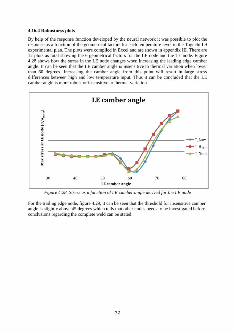
72
4.16.4 Robustness plots
By help of the response function developed by the neural network it was possible to plot the
response as a function of the geometrical factors for each temperature level in the Taguchi L9
experimental plan. The plots were compiled in Excel and are shown in appendix III. There are
12 plots as total showing the 6 geometrical factors for the LE node and the TE node. Figure
4.28 shows how the stress in the LE node changes when increasing the leading edge camber
angle. It can be seen that the LE camber angle is insensitive to thermal variation when lower
than 60 degrees. Increasing the camber angle from this point will result in large stress
differences between high and low temperature input. Thus it can be concluded that the LE
camber angle is more robust or insensitive to thermal variation.
Figure 4.28. Stress as a function of LE camber angle derived for the LE node
For the trailing edge node, figure 4.29, it can be seen that the threshold for insensitive camber
angle is slightly above 45 degrees which tells that other nodes needs to be investigated before
conclusions regarding the complete weld can be stated.
30 40 50 60 70 80
Ma
x s
tre
ss a
t L
E n
od
e [σ
/σ
no
rm]
LE camber angle
LE camber angle
T_Low
T_High
T_Nom

73
Figure 4.29. Stress as a function of LE camber angle derived for the TE node
The same methodology can be used to investigate the remaining geometrical factors shown in
appendix III. A large span between low and high temperature reveals that the particular
geometrical setting is sensitive to variation in temperature and therefore the topology needs to
be defined with caution.
0 20 40 60 80 100Ma
x s
tre
ss a
t T
E n
od
e [
σ/σ
no
rm]
LE camber angle
LE camber angle
T_low
T_high
T_nom
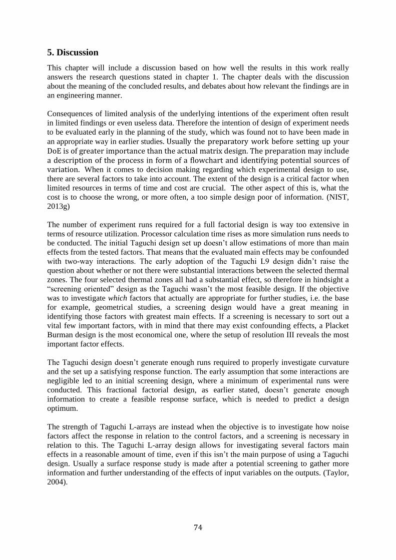
74
5. Discussion
This chapter will include a discussion based on how well the results in this work really
answers the research questions stated in chapter 1. The chapter deals with the discussion
about the meaning of the concluded results, and debates about how relevant the findings are in
an engineering manner.
Consequences of limited analysis of the underlying intentions of the experiment often result
in limited findings or even useless data. Therefore the intention of design of experiment needs
to be evaluated early in the planning of the study, which was found not to have been made in
an appropriate way in earlier studies. Usually the preparatory work before setting up your DoE is of greater importance than the actual matrix design. The preparation may include a description of the process in form of a flowchart and identifying potential sources of variation. When it comes to decision making regarding which experimental design to use,
there are several factors to take into account. The extent of the design is a critical factor when
limited resources in terms of time and cost are crucial. The other aspect of this is, what the
cost is to choose the wrong, or more often, a too simple design poor of information. (NIST,
2013g)
The number of experiment runs required for a full factorial design is way too extensive in
terms of resource utilization. Processor calculation time rises as more simulation runs needs to
be conducted. The initial Taguchi design set up doesn’t allow estimations of more than main
effects from the tested factors. That means that the evaluated main effects may be confounded
with two-way interactions. The early adoption of the Taguchi L9 design didn’t raise the
question about whether or not there were substantial interactions between the selected thermal
zones. The four selected thermal zones all had a substantial effect, so therefore in hindsight a
“screening oriented” design as the Taguchi wasn’t the most feasible design. If the objective
was to investigate which factors that actually are appropriate for further studies, i.e. the base
for example, geometrical studies, a screening design would have a great meaning in
identifying those factors with greatest main effects. If a screening is necessary to sort out a
vital few important factors, with in mind that there may exist confounding effects, a Placket
Burman design is the most economical one, where the setup of resolution III reveals the most
important factor effects.
The Taguchi design doesn’t generate enough runs required to properly investigate curvature
and the set up a satisfying response function. The early assumption that some interactions are
negligible led to an initial screening design, where a minimum of experimental runs were
conducted. This fractional factorial design, as earlier stated, doesn’t generate enough
information to create a feasible response surface, which is needed to predict a design
optimum.
The strength of Taguchi L-arrays are instead when the objective is to investigate how noise
factors affect the response in relation to the control factors, and a screening is necessary in
relation to this. The Taguchi L-array design allows for investigating several factors main
effects in a reasonable amount of time, even if this isn’t the main purpose of using a Taguchi
design. Usually a surface response study is made after a potential screening to gather more
information and further understanding of the effects of input variables on the outputs. (Taylor,
2004).

75
When deciding what nodes that was to be chosen for analysis it quickly became clear that area
of analysis had to be reduced in order to grasp the problem. The response function developed
in this report does only provide a model for stress amplitudes in the leading edge node.
Taking other nodes into consideration will change the composition of the model, but this
report suggest a methodological approach on how such a model can be created.
When looking on a main effect plot it is important to remember that the plot only shows
results in terms of data means and does not represent the actual effect at a certain time step in
the flight cycle. Another time step will most certain show another relationship for the main
effects. A better understanding was gained by interpreting the effect of different thermal
zones in each time step for all nodes along the suction side weld.
The effect of the thermal zones cannot be estimated independently from each other, in conflict
with the assumptions for the initial DoE set up. The interaction plots for the Taguchi L9
experimental plan showed that there were interactions between the thermal zones, but the
additional study with the Box-Behnken experimental plan showed that there weren’t any
interaction effects, which provided a puzzling result. Nevertheless the Taguchi L9 interaction
plots cannot be trusted since there are confounding effects within the experimental plan. For
future work there should be an initial DoE without confounding factors to detect main effects
and at least second order interactions. This was presented with the presented Box-Behnken set
up. With few experimental runs it was difficult to determine what temperature differences that
were the most significant stress drivers. The data behaved stochastic and thus it was difficult
to see any patterns in the plotted data. Further experimentation and a larger experimental plan
with no confounding effect are needed to search for these stress drivers in a beneficial way.
Validation test runs needs to be performed in order to be sure that the model behaves as
predicted. One also needs to evaluate to what level the R-squared statistics actually answers
whether a model is good or not. An overall consensus in the engineering society is that a high
R-square and a low P-value guarantees that you have a good model, which in fact is not
always the case. It is important to analyze how the residuals are distributed and perform test
runs with other data in order to verify that the model behaves well. A model for the reduced
flight cycle was not considered in this thesis, but is also an interesting area of investigation.
5.1 Improvement of analysis procedure
Together with the experienced engineers in the EWB group an analysis procedure was
developed which significantly reduced simulation time and facilitated the post processing of
data. A Python-script was written that performs all analyses in an automated way and gathers
the results in a collected result file. Procedures on how to interpret DoE data have been
presented which eases post processing of the DoE data in a structured way. Predefined edges
and lines have been implemented in the CAD models to ease the choice of nodes in the
ANSYS-scripts. The new predefined edges are shown in figure appendix IV.
The thermal analyses can also be performed in stationary mode which also saves simulation
time to a tenth of the original. For an initial study based on DoE related work this is a
beneficial way to shorten the simulation time.
The use of MATLAB showed weaknesses in automatic post processing since MATLAB code
could not be executed on a remote server. The graphical interface had to be used to run the

76
scripts which hampered post processing operations. Other software might function in a more
beneficial way, which needs to be investigated.
The use of R-square statistics needs to be performed with caution. The overall consensus
regarding the R-square and the P-value is that a high R-square and low P-value automatically
shows that the model is good, which is not the actual case. A low R-square value can be
calculated for a model that actually fits the data well and a high R-square value can be
calculated for a model that does not fit the data at all. Similar relationships exist for the P-
value. A low p-value does not necessary mean that the model has a good fit. A further
analysis of the residuals and the actual F-value gives a greater understanding of the model and
are powerful techniques for model evaluation. Validations test runs are also needed to make
sure that the model behaves well.

77
6. Sources of error
The simulations performed in this thesis work used predefined finite element models with
predefined mesh sizes. The results of this analysis could have been more precise if another
mesh size had been used. If smaller elements had been used the results would have been more
precise with the drawback of longer simulation time. The finite element method models used
in the analysis were shell models which try to replicate solid models by applying stiffness to
each element. A solid FEM model would on the other hand increase the simulation time. No
consideration has been taken to how stiffness is affected by increasing temperature levels.
Thus the effect of changing material properties has not been investigated.
The initial settings for thermal variation set points was ±28K, based on engineering
experience and considered feasible in line with knowledge from earlier projects. (Arroyo,
2014)
A different approach for this would be to set the levels for the temperature variance as a limit
at a certain distance from the standard deviation of the thermal distribution. A suggestion is
the setting for ∆𝑇 as;
∆𝑇 = µ + 3𝜎
Here µ is the mean temperature value of data and 𝜎 is the standard deviation.
The applied temperatures for the analyses are based on air temperatures in the different
thermal zones and originally from OEM, which is the “source of variation”. The transient
temperatures that occur between the air temperature and the actual temperature in the metal
surfaces will affect the results. If calculations are made directly from metal temperatures more
reliable results would have been obtained for the stresses. For this particular study the air
temperatures represent the input data from OEM, which makes it relevant as the investigated
variance parameters. Next question may be if the received OEM data really is best suited as
base for a DoE, where a distinct effect from a certain parameter is wanted. Maybe a heavier
weighting (larger values on the selected levels) of the original data or a more “extreme” data
would have uncovered effects and behaviors that are hard to discover with the current data
from a real flight cycle.
The choice of DoE setup in this thesis work is not fully investigated and there may be better
design settings. A different design setup is suggested in future works, but everything depends
on what one wants to accomplish with the study and what the objective is. As discussed, the
initial choice of a Taguchi design left out some important information that could have been
investigated at an earlier stage.

78
7. Conclusion
Consequences of limited analysis of the underlying intentions of the experiment often result
in limited findings or even useless data. Therefore the intention of the experiment and a clear
objective of the study need to be evaluated early in the planning of the experimental design
set up.
The conflict between the economic benefits of running factorial screening designs and the
lack of information about possible two-factor interactions is ultimately a question of priorities
and what the impact may be if the interpreted results are not correct. As stated in discussion
chapter, the Taguchi design methods have the benefits that you can sort the experimental plan
in controllable and uncontrollable variation. This was used as an initial approach to the
project, but later the idea of Taguchi design was considered unnecessary because of the
insight that in computer simulations the experiments are deterministic, which means that all
parameters are controllable, even the noise factors (Forslund, 2012). This leads to the
conclusion that the Taguchi L9 could be replaced with a regular suitable fractional factorial
design, if the main effects are of interest and a screening design is needed. For a highly
saturated factorial screening the Placket Burman design is more feasible when it comes to the
investigation of many factors, and the so called Pareto principle applies. Pareto principle
states that, in relation to the investigation of factors, that around 80% of the effects comes
from 20% of the factors, even called “law of the vital few” or “the principle of factor
sparsity”. The Pareto principle is applicable when it comes to the investigation of many
different factors, where it is most likely only some of the factors that have substantial effect.
This could be the case when you, for example, have a lot of different geometrical parameters
to try out. For future work there should be an initial DoE without confounding factors to
detect main effects and at least second order interactions if this is the objective of the study.
The investigated effect plots from the different thermal zones indicated a non-linear behavior,
which indicate that Designs of Experiments with at least three levels should be used to
investigate this even further. A model that best describe what type of curvature that is present
within the response is needed.
A study of a Box-Behnken design was conducted which showed that the models were slightly
improved, but that there were still an insignificant fit against the response data. Conclusion
that could be drawn from this was that there are other factors contributing to increased stress
levels other than only temperature gradients. The Box-Behnken experimental plan showed
equal results in main effects as the Taguchi L9 experimental plan.
During the initiating phases of this thesis work it was early found that there was no
standardized way of investigating stress levels at different welds on the TS. The nodes on the
lower suction side weld edge had to be picked manually in ANSYS, making it time
consuming to investigate other weld edges or positions of interest on the TS.
The factors with substantial main effects are chosen for a more in depth analysis in response
surface methodology where it is possible to study the factors with help of statistical tools such
as regression and ANOVA analysis. The results can also be used for optimization purposes.
The performed screening design also confirms this with the given results in 4.17.3. Which
implies that in our system, there are a few driving factors as can be seen in figure 4.17. As
presented in the figure with help of the Neural Network Function the axial chord length has a

79
large effect on the generated stress level, and should therefore be further investigated in
additional studies. There are confounding effects within the response function which also
needs to be addressed before using the Neural Network Function for decision making
purposes. The geometrical study does not consider maximum or minimum stresses at other
positions in the TS and the neural network function has not been evaluated for its lack of fit.
From the geometrical study it could also be concluded that the LE chamber angle is more
robust or insensitive to thermal variation for degrees lower than 60. The curvature within the
robustness plots can be a result of the interpolation occurring within the neural network
function. Therefore the threshold for insensitive geometrical factors settings needs to be
investigated further before conclusions regarding overall robustness can be stated.
A large span between low and high temperature reveals that the particular geometrical setting
is sensitive to variation in temperature and therefore the topology needs to be defined with
caution.
ANSYS-script, Python-script and post processing code has been written that supports further
investigation of other welds at predefined nodes in the TS. It was also not possible to use
MATLAB for the automated post processing operations, which will be mentioned in
following chapters.

80
8. Developed methodology for investigation of thermal robustness
Addressing the research question in this thesis report the major outcome of this thesis is the
methodology implemented and investigated during this work. The following procedures serve
as a suitable approach on how to increase thermal robustness of the TS:
1. Gather information about the problem and investigate what thermal loads those are to
be studied.
2. Define the objectives of the study, determine what experiment approach is appropriate
and select the process variables. The result of design of experiment is much depending
on what choices that are made on this level. A support for additional DoE studies has
been created and recommendations for different experimental plans have been shown
that serve different experimental purposes.
3. Predefined node positions which support possibility to investigate different geometries
and different weld or edges on the struts have been created.
4. An automated analysis procedure developed for the purpose of performing many
experimental runs in a short time are always needed. Simulation time can be shortened
by the use of ANSYS-script, Python-scripts and automated post processing operations
mentioned in this thesis report. Automated generation of BC-tables also support in the
reduction of simulation time.
5. The key design parameters can be identified by analysing main effect plots and
interaction plots, but the key issue is that the chosen experimental plan has to be
chosen with care, depending on what objective you have with the study. If a large set
of potential parameters needs to be investigated, a screening design may be
appropriate to distinguish key parameters for further, more in-depth investigation.
When those important factors are identified, a surface response objective may be
appropriate to get a more extensive understanding of the behaviors of those parameters
and their effects.
6. Regression or ANOVA analysis can be performed to develop response functions that
can be used in many ways to answer the objectives of the experiment.
7. The method used for the geometrical attributes can be used to gather knowledge on
how to increase robustness with respect to thermal and geometric attributes. Neural
network functions serve as a good way of identifying which geometrical parameters
that are sensitive together with the effects of the thermal zones and is also beneficial
for combining results from several studies.
8. This thesis work suggests DoE experimental plans that can be used for screening and
development of response functions all of which are applicable early in the product
development processes.

81
9. Further work
Suggestions for further work are here presented, based on conclusions drawn from this thesis
work.
A methodology was developed to be able to analyse several predefined welds. Unfortunately
these welds could not be studied within this thesis due to the lack of time for multiple studies.
In the interest of GKN it would be beneficial to study how thermal BC’s affect stress
distribution along all of these welds. It would support a better understanding of the design and
also prove beneficial in terms of optimizing the component. For this work the material data
wasn’t specified to simulate a real weld, which in some way should be the goal for future
studies. Weld simulations could be implemented and data from such simulations could be
used in further studies.
Validation test runs need to be implemented in the future to validate that the response
function works as anticipated.
The DoE analysis process, that has been presented, is an extensive and iterative process. It is
reprehensible to draw conclusion based on experimental results if the experimental plan itself
from which the runs are generated are incorrect processed. A methodology for analysis of
DoE data has been presented as well as techniques that can be used for development of a
response function. Stepwise regression can be used to develop response functions for different
response variables of choice by using the DoE analysis flowchart. A single response function
including data measurements from several nodes from the model have not been developed,
but would be of high interest for a follow up on this thesis. A response function that shows
stress as a function of several observation points at different positions on the TS is well suited
for multi-objective optimization purposes. That is as long as the underlying DoE analysis
have been done in a correct way and that reasonable conclusions have been made, a work that
has been much regarded in this thesis, but needs further investigation.
As stated in conclusion, today the BC-tables that correspond the input from OEM, have to be
updated manually if changes are needed. In the future an easy-operated automatic update of
the BC-tables is appropriate for a more efficient iterative process. A proposal is
implementations of BC-tables in the python-script, where a single command could be used to,
for example, change the weightings of all temperatures. In this thesis work the data from a
real flight cycle was used, but in further projects the practitioner may want to use more
extreme data, or custom made data to investigate certain interests.
All of the work related to MATLAB was done in the graphical interface of the software.
Today, post processing is made manually in this interface which doesn’t support a fast
evaluation of the results. In order to speed up post processing, investigation is needed to
answer if it is possible to use MATLAB on a remote server for post processing purposes.
Other software’s might be more useful for this purpose and those need to be investigated and
weighted against their pros and cons. Some built in functions of the MATLAB code doesn’t
support other DoE setups than Taguchi L9. There are many possibilities for improvements of
the post processing MATLAB code.
In this study the main effects for the geometry parameters were generated from ModeFrontier,
but in future studies a correct design of experiment set up should be implemented. Design set
ups suitable for future research could be Latin Hypercube, space filling or Definitive

82
screening design in Jmps, to name a few. The current Python-script works well for a Taguchi
L9 design, but still needs further work to implement other experimental designs. During this
project a wide range of software was utilized, but the potential of this software should be
more investigated. To name an example the comparison between MINITAB and Jmp, for
DoE generation and statistical tools, should be investigated. Even the exploration of other, not
utilized software, should be made in future projects.
To minimize simulation time, in future studies, only the temperature difference with the
highest impact on stress levels should be chosen as a factor. For example, an increase in the
temperature difference between Zone 2 and Zone 4 has strong correlation with higher stresses
in the component, and should therefore be tested as the only contributing factor in the DoE
setup. This factor would then be given a high or a low value, and through how distinct the
interaction effect is, to each different geometrical factor, one can investigate which
geometrical configuration would result in a high sensitivity to generated stresses.
83
10. References
Aerospace, G., 2014. GKN. [Online] Available at: http://www.gkn.com/aerospace/aboutus/Pages/Vision-and-strategy.aspx
Aerospace, G., 2014. GKN. [Online] Available at: http://www.gkn.com/aerospace/aboutus/Pages/default.aspx
Aerospace, G., u.d. VOLS:10072673, Trollhättan: GKN Aerospace Engine Systems.
Arroyo, C., 2014. Aerothermaldynamics engineer [Intervju] (Februari 2014).
Assarlind, D. M., 2014. Quality and Operations Mangement [Intervju] (14 May 2014).
Benjamin S. Blanchard, W. J. F., 1990. System Engineering and Analysis. 2nd Edition red. New Jersey: Prentice-Hall, Inc..
Buydens, L., u.d. Webchem.science.ru.nl. [Online] Available at: http://www.webchem.science.ru.nl/cgi-bin/Stat/XPD/xpd2.pl
Forslund, A., 2012. Optimization of Geometric Robustness of Aero Structures in Early Design Phases, Gothenburg: Department of Product and Production Development, Chalmers University of Technology.
Kuehl, R. O., 2000. Design of Experiments: Statistical Principles of Research Design and Analysis. 2nd red. Pacific Grove, USA: Duxbury, Thomson Learning.
Kutz, M., 2009. Eshbach's Handbook of Engineering Fundamentals. Fifth Edition red. u.o.:John Wiley & Sons..
Lundh, H., 2000. Grundläggande hållfasthetslära. Third Edition red. Stockholm: Instant Book AB.
MathWorks, 2014. MathWorks Inc.. [Online] Available at: http://www.mathworks.se/products/neural-network/description3.html [Used 31 May 2014].
Meier, L., 2013. Statistical and Numerical Methods for Chemical Engineers. [Online] Available at: http://stat.ethz.ch/~meier/teaching/cheming/cheming-e-part-II.pdf [Used 26 May 2014].
Mukhopadhyay, A. I. K. a. S., 2010. Response Surface Methodology. WIREs Computional Statistics, Volym 2, pp. 128-149.
NIST, 2012. Engineering Statistics Handbook. [Online] Available at: http://www.itl.nist.gov/div898/handbook/pri/section5/pri593.htm [Used 19 May 2014].
NIST, 2012g. NIST/SEMATECH e-Handbook of Statistical. [Online] Available at: http://www.itl.nist.gov/div898/handbook/prc/section1/prc131.htm [Used 28 May 2014].

84
NIST, 2012h. NIST/SEMATECH e-Handbook of Statistical Methods. [Online] Available at: http://www.itl.nist.gov/div898/handbook/pmd/section4/pmd44.htm [Used 03 June 2014].
NIST, 2012i. NIST/SEMATECH e-Handbook of Statistical Methods. [Online] Available at: http://www.itl.nist.gov/div898/handbook/pmd/section4/pmd445.htm [Used 03 June 2014].
NIST, 2012. NIST/SEMATECH e-Handbook of Statistical Methods. [Online] Available at: http://www.itl.nist.gov/div898/handbook/pri/section4/pri43.htm [Used 31 May 2014].
NIST, 2012. NIST/SEMATECH e-Handbook of Statistical Methods. [Online] Available at: http://www.itl.nist.gov/div898/handbook/pri/section4/pri41.htm [Used 31 May 2014].
NIST, 2013a. NIST/SEMATECH e-Handbook of Statistical Methods.. [Online] Available at: http://www.itl.nist.gov/div898/handbook/pmd/section3/pmd31.htm [Used 2014].
NIST, 2013b. NIST/SEMATECH e-Handbook of Statistical Methods. [Online] Available at: http://www.itl.nist.gov/div898/handbook/pri/section1/pri13.htm [Used 2014].
NIST, 2013c. NIST/SEMATECH e-Handbook of Statistical Methods. [Online] Available at: http://www.itl.nist.gov/div898/handbook/pri/section3/pri3344.htm [Used 04 June 2014].
NIST, 2013d. NIST/SEMATECH e-Handbook of Statistical Methods. [Online] Available at: http://www.itl.nist.gov/div898/handbook [Used 10 May 2014].
NIST, 2013e. NIST/SEMATECH e-Handbook of Statistical Methods. [Online] Available at: http://www.itl.nist.gov/div898/handbook/pri/section3/pri3362.htm
NIST, 2013f. NIST/SEMATECH e-Handbook of Statistical Methods.. [Online] Available at: http://www.itl.nist.gov/div898/handbook/pri/section3/pri335.htm [Used 2014].
NIST, 2013. NIST/SEMATECH e-Handbook of Statistical Methods. [Online] Available at: http://www.itl.nist.gov/div898/handbook/pri/section3/pri33.htm [Used 2014].
NIST, 2013. NIST/SEMATECH e-Handbook of Statistical Methods. [Online] Available at: http://www.itl.nist.gov/div898/handbook/prc/section4/prc43.htm [Used 2014].
Norrby, P., 2012. Prediction of coast-down test results, Gothenburg: Chalmers University of Technology.

85
Rama Rao. S, P. G., 2012. Application of Taguchi methods and ANOVA in optimization of process parameters for metal removal rate in electrochemical machining of Al/5%SiC composites. International Journal of Engineering Research and Applications (IJERA), Vol.2(Issue 3), pp. 192-197.
Simpson, J. R. S. &. C. M. &. G. T. H., 2013. Gudielines for Planning and Evidence for Assessing a Well-Designed Experiment. i: Quality Engineering. Eglin, Florida: Taylor & Francis, pp. 25:4, 333-355.
Taylor, D. W., 1991. Optimization and Variation Reduction in Quality. u.o.:McGraw-Hill.
Taylor, D. W., 2004. Quality Management Systems - Process Validation Guidance, u.o.: The Global Harmonization Task Force.
Ulrich, K. &. E. S., 2011. Product Design and Development. 5 red. u.o.:McGraw-Hill Higher.
Vilmart, T., 2010. Probabilistic Life Prediction of an Airplane Engine Component, Gothenbyrg, Sweden: Chalmers university of Technology.
Winter, B., 2014. The F distribution and the basic principle behind ANOVAs. [Online] Available at: http://www.bodowinter.com/tutorial/bw_anova_general.pdf [Used 30 May 2014].
Wu. C.F. Jeff, H. M., 2000. Experiments: Planning, analysis, and parameter deisgn optimization. i: New York: Wiley: u.n., p. 112.

86
Appendix I
CONFIDENTIAL MATERIAL

87
Appendix II
CONFIDENTIAL MATERIAL

88
Appendix III
CONFIDENTIAL MATERIAL

89
Appendix IV
CONFIDENTIAL MATERIAL

90
Appendix V
CONFIDENTIAL MATERIAL