increasing lifetime of oil production tubings
TRANSCRIPT

Increasing Lifetime ofOil Production Tubings
Wiener Neustadt, May 2007 David Doppelreiter

Department of General, Analytical and Physical
Chemistry,University of Leoben
David Doppelreiter May 2007
Increasing Lifetime of Oil Production Tubings

Acknowledgement
I would like to express my gratitude to my care Assoc. Prof. Dr. Gregor Mori for giving me the opportunity to write this thesis on the department of General, Analytical and Physical Chemistry at the University of Leoben in cooperation with the OMV AG.
I would also like to thank my advisor Dr. Markus Oberndorfer, Expert in the field of corrosion and Head of the Laboratory of Exploration and Production at OMV Exploration & Production GmbH for his help and support during my work on this project. Many thanks are extended to Dr. Wolfgang Havlik and DI Karin Thayer, who always supported me in different kinds of questions during this project.
I also owe thanks to the whole team of the Laboratory for Exploration and Production for their overall support, especial Mr. Leopold Steinmayer for his technical support during the testing procedure and Mag. Wolfgang Hujer for analysing my samples via Scanning Electron Microscope.
Furthermore I express my special gratitude to my parents for the possibility to go for this study and their fantastic support during it. Finally I would like to thank my girlfriend Irene for her great help in many difficult times and her delightful encouragements during the last years in several parts of my life and for carefully reviewing the manuscript.
David Doppelreiter Table of contents
I
Table of contents
1 Introduction 12 Oil production with subsurface sucker rod pumps 5
2.1 Subsurface sucker rod pump 5
2.2 Corrosion in subsurface sucker rod pumps 9
2.3 Lining of tubing - swagelining 11
2.4 Tribology of polymer materials 13
2.4.1 What means tribology? 13
2.4.2 Contact mechanics between solids 15
2.4.3 Friction and wear of polymers 23
2.4.3.1 Classification of polymers 24
2.4.3.2 Structure and properties of thermoplastic materials 24
2.4.3.3 Thermoplastic materials 31
2.4.3.4 Adhesion 34
2.4.3.5 Friction 36
2.4.3.6 Wear 42
2.4.3.7 Abrasive Particles 47
3 Experimental Operation 523.1 Materials 52
3.1.1 Polymers for lining 52
3.1.2 Couplings 58
3.1.3 Rod centralizer 60
3.2 The pilot plant 61
3.3 Testing procedure 63
3.4 Testing parameters 63
3.5 Evaluation of materials and specimens 65
3.5.1 Shore D Durometer 65
3.5.2 Chromatic coding confocal sensor 66
3.5.3 Evaluation by Mathematika 67
3.5.4 Scanning electron microscopy 68
3.5.5 Tensile testing 69

David Doppelreiter Table of contents
II
3.5.6 Heat-Chemical Treatment 70
4 Results 714.1 Measured values by the use of chromatic coding confocal sensor 71
4.2 Measured values by the use of a shore (D) durometer 75
4.3 Measured values by the use of a tensile testing machine 75
4.4 Values given by Borealis 75
4.5 Calculated values 75
4.6 Interrelationship of results and different polymer properties 75
4.7 Scanning Electron Microscopy 75
5 Discussion 755.1 Sliding contact of polymer samples versus spray metal couplings 75
5.2 Sliding contact of polymer samples versus spray metal couplings
including sand particles in the medium 75
5.3 Sliding contact of polymer samples versus polyamide rod centralizer 75
5.4 Sliding contact of polymer samples versus polyamide rod centralizer
including sand particles in the medium 75
6 Conclusion 757 Outlook 758 Appendix 75
8.1 Appendix A 75
9 Literature 75

David Doppelreiter Introduction
1
1 Introduction
After a successful drilling job and if the natural pressure of the deposit is not high enough the well goes into production by an artificial lifting system. The oil production in Austria (OMV) is characterized by a wide variety of conveyor techniques. The most popular technique (> 60%) to lift crude oil on the continent is the subsurface sucker rod pump. In Europe more than 90% of all wells are equipped with this kind of artificial lift method. The reason for this popularity is the operating efficiency, the flexibility and the broad application as well as the uncomplicated and rapid installation. But there are also problems due to corrosion and wear causing well-failures, especially of tubings (most common and expensive failure), strings and pumps, and consequently production loss and work over costs.
For understanding the problems it is necessary to view more detailed the lifted medium, the characteristic of a borehole, and the sucker rod unit. The lifted medium (crude oil) is placed in a reservoir rock (sandstone) and is a mixture of oil, water and sand. Therefore it is a very corrosive medium for the metal parts in a sucker rod pump due to the formation water with its content of chlorides, sulfides and dissolved gases (H2S, CO2 or SO2). The appearance of sand particles (0-1%) which are generated due to the inflow of the oil mixture to the pump is shortening lifetime and can be more dramatically if wrong acidizing destroys the formation. The deviation of boreholes is causing more wearing contact of the rod, coupling and the tubing wall and produces more abrasion. Because of the high depth of a well (2 - 3km) and the resulting high length of the rod, a rod centralizer is essential to minimize the deformation and thus increases lifetime.
The average runtime of one sucker rod pump in Austria is currently about 1200 days and has been increasing dramatically in the past 50 years. For instance the runtime in 1958 was about 80 days. Due to the development of specific technology improvements the lifetime of sucker rod units increased especially in the 80ies up to now. This success was achieved by corrosion protection with proper inhibitors, by optimization of tubing, sucker rod and coupling (e.g. spray metal) materials, sand wires, and by a consequent corrosion monitoring.Increasing lifetime would save a great amount of money and would raise the oil production enormously in case of using approximately 10.000 sucker rod units by the OMV (covering Austria and Romania).

David Doppelreiter Introduction
2
As mentioned before tubing failures are the most common and expensive ones. The actual root cause of tubing failures has been a synergistic effect of both the rods wearing on the tubing wall coupled with the electrochemical attack of the environment. This is apparent because neither the calculated wear rates nor the measured corrosion rates alone would allow such rapid metal loss of the tubing wall in such a short time period.In the last years sucker rod completions using tubings with thermoplastic liner pipes were successfully installed to avoid corrosion at the tubing generally. The better corrosive properties of the polymers are contrary to unknown tribological properties under contact with couplings of different roughness (0,1 - 3µm) and rod centralizer.Apart from better corrosion properties and therefore increasing lifetime even more benefits appear like less consumption of electricity (15-20%) due to decreased friction, applicability in used tubings as well as less paraffin wax segregation as a result of minimized temperature loss.
Because of all these promising benefits this thesis should examine the wear behaviour of different thermoplastic polymers through tribological tests under real conditions (oil, water, salt and sand) in a pilot plant.
The following pictures should give a small and fast overlook about the sucker rod pump unit and the common problems during operation (see Figure 1.1).

David Doppelreiter Introduction
3

David Doppelreiter Introduction
4
Figure 1.1: Overlook about a subsurface sucker rod pumping unit and the common problems during operation.
David Doppelreiter Oil production with subsurface sucker rod pumps
5
2 Oil production with subsurface sucker rod pumps
2.1 Subsurface sucker rod pump
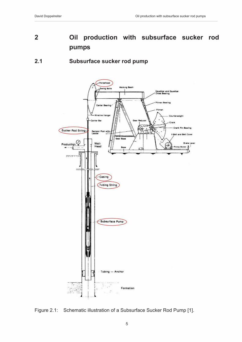
Figure 2.1: Schematic illustration of a Subsurface Sucker Rod Pump [1].
David Doppelreiter Oil production with subsurface sucker rod pumps
6
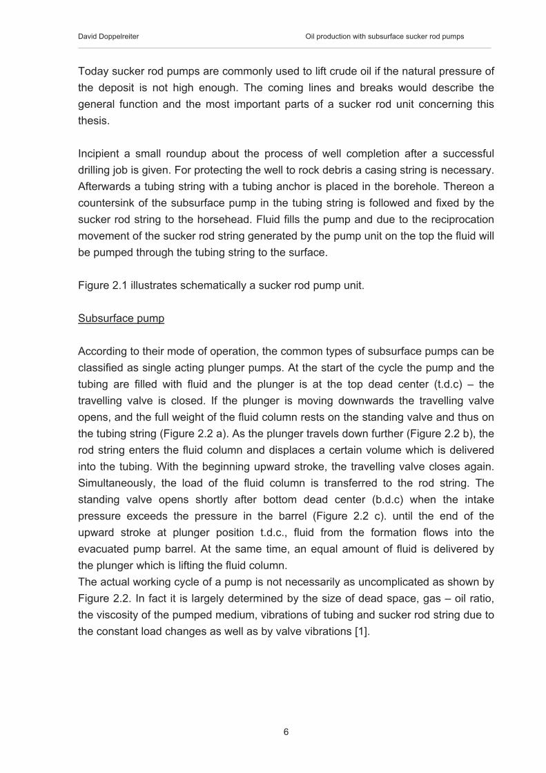
Today sucker rod pumps are commonly used to lift crude oil if the natural pressure of the deposit is not high enough. The coming lines and breaks would describe the general function and the most important parts of a sucker rod unit concerning this thesis.
Incipient a small roundup about the process of well completion after a successful drilling job is given. For protecting the well to rock debris a casing string is necessary. Afterwards a tubing string with a tubing anchor is placed in the borehole. Thereon a countersink of the subsurface pump in the tubing string is followed and fixed by the sucker rod string to the horsehead. Fluid fills the pump and due to the reciprocation movement of the sucker rod string generated by the pump unit on the top the fluid will be pumped through the tubing string to the surface.
Figure 2.1 illustrates schematically a sucker rod pump unit.
Subsurface pump
According to their mode of operation, the common types of subsurface pumps can be classified as single acting plunger pumps. At the start of the cycle the pump and the tubing are filled with fluid and the plunger is at the top dead center (t.d.c) – the travelling valve is closed. If the plunger is moving downwards the travelling valve opens, and the full weight of the fluid column rests on the standing valve and thus on the tubing string (Figure 2.2 a). As the plunger travels down further (Figure 2.2 b), the rod string enters the fluid column and displaces a certain volume which is delivered into the tubing. With the beginning upward stroke, the travelling valve closes again. Simultaneously, the load of the fluid column is transferred to the rod string. The standing valve opens shortly after bottom dead center (b.d.c) when the intake pressure exceeds the pressure in the barrel (Figure 2.2 c). until the end of the upward stroke at plunger position t.d.c., fluid from the formation flows into the evacuated pump barrel. At the same time, an equal amount of fluid is delivered by the plunger which is lifting the fluid column. The actual working cycle of a pump is not necessarily as uncomplicated as shown by Figure 2.2. In fact it is largely determined by the size of dead space, gas – oil ratio, the viscosity of the pumped medium, vibrations of tubing and sucker rod string due to the constant load changes as well as by valve vibrations [1].

David Doppelreiter Oil production with subsurface sucker rod pumps
7
Figure 2.2: Schematic drawing of a pumping cycle [1]. Top dead center (t.d.c) Bottom dead center (b.d.c)
Sucker rod string, couplings and centralizers
The sucker rod string is connecting the pumping unit on the top and the subsurface pump which is anchored in the reservoir. Each rod (depending on the shaft diameter) has a length of about 9000 mm and is interconnected with steel couplings (Figure 2.3). In compliance with API Specification 11B, sucker rods are only distinguished by tensile strength values (different steel grades). Sucker rod centralizers (or protectors) are used for centralizing the rod string, during the reciprocation movement in the tubing string, and for mechanical removal of paraffin deposits. The rod centralizers are made of high wear resistant polyamide (including Teflon for improving friction behaviour) which shows excellent anti-frictional properties and absolute resistance to oil and water attack at temperatures up to 100°C max. After careful preparation of the rods without damaging its surface, centralizers are sprayed on at temperatures close to 300°C. The following protectors are sprayed on at a stroke length distance but offset by 45°.Because of reciprocation movement and borehole deviations the couplings and the protectors are in sliding contact with the inside wall of the tubing string. This is resulting in friction (energy loss) and wear (material loss). In the past years OMV was

David Doppelreiter Oil production with subsurface sucker rod pumps
8
testing different types of couplings to reduce friction and wear for the tubing wall as well as for the coupling itself. After these steps the new type of coupling (spray metal coupling) shows less roughness (Ra = 0,1 µm) and much higher corrosion resistance compared to the old unalloyed coupling (Ra = 3 µm). [1]
Figure 2.3: Rod connection via coupling [1].
Figure 2.4: Rod centralizer [1]
Tubing string
Already during drilling operations it is necessary to install a casing string to protect the well from difficult well sections and other problems like leaching, chunking and unwanted disruptions from the rock mass. The accruing annulus between casing and rock mass will be filled up with cement. This cementation is necessary for a body contact between the casing and the rock mass to transfer forces, for corrosion prevention and for the isolation of permeable formations.

David Doppelreiter Oil production with subsurface sucker rod pumps
9
After a finished drilling operation and an installed casing a tubing string is inserted for conveying the medium. The subsurface pump and the rod string are placed inside of the tubing string (Figure 2.1) and after starting the pumping unit aboveground oil production is beginning.
Figure 2.5: Tubings (OMV tube storage Prottes, Austria)
2.2 Corrosion in subsurface sucker rod pumps
Corrosion is the reaction of the material with its environment that yields to a degradation of the material. Type of the reaction can be chemical, electrochemical and physical. In many cases corrosion is the inversion of metallurgy. Corrosion reactions of metals in most cases consist of two half reactions:
An oxidation, which is the corrosion process,
Me � Me2+ + 2 e- (Equ. 2.1)
and a reduction of an oxidant e.g.,
2 H+ + 2 e- � H2 (Equ. 2.2)

David Doppelreiter Oil production with subsurface sucker rod pumps
10
Oxidation takes place at the anode, reduction at the cathode. Chemical corrosion occurs, when both reactions happen at the same place while in the case of electrochemical corrosion both reactions are separated. A distance of some atomic layers is sufficient [2].
In petroleum operations corrosion is inevitable. The formation water with its content of chlorides, sulfides and dissolved gases (H2S, CO2 or SO2) which is pumped up with the oil represents an ideal electrolyte. Due to potential differences of individual materials, an electrical current starts to flow which is proportional to the metal removal at the anode. In field operation the following major types of corrosion occur:
� Uniform corrosion � Pitting corrosion � Galvanic corrosion between metals of different types and alloying
composition� Intergranular corrosion � Stress corrosion cracking � Erosion corrosion � Crevice corrosion
The formation of areas with different potential (anode, cathode) and consequently the flow of electric current and the occurrence of corrosion phenomena is the result of a number of causes:
� Surface damages (e.g. wrench nicks, hammer marks, scores) � Insufficient material homogeneity � Increased material stresses due to local plastic deformation � Damages to corrosion inhibiting coating � Lubricant residue [1]
Because of the inevitable corrosion due to formation water it is necessary to find solutions to protect the production equipment. One opportunity is the introduction of inhibitor substances into the lifted medium to guard the equipment from corrosion during production operations. An inhibitor is a substance which retards or slows down a chemical reaction. Thus, a corrosion inhibitor, when added to an environment, decreases the rate of attack by the environment on a metal. Corrosion inhibitors are commonly added in small amounts to acids, cooling waters, steams and other environments, either continuously or intermittently to prevent serious corrosion. It would be awkward to include
David Doppelreiter Oil production with subsurface sucker rod pumps
11
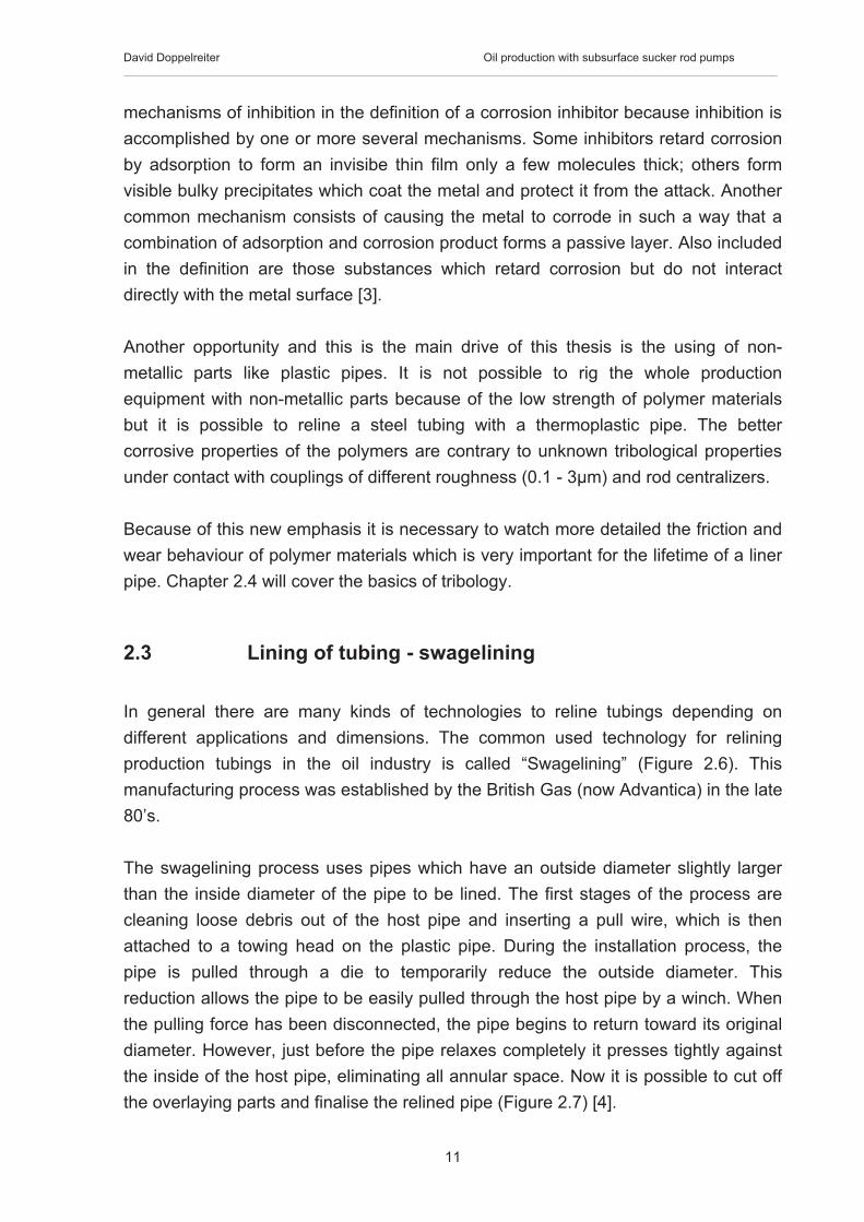
mechanisms of inhibition in the definition of a corrosion inhibitor because inhibition is accomplished by one or more several mechanisms. Some inhibitors retard corrosion by adsorption to form an invisibe thin film only a few molecules thick; others form visible bulky precipitates which coat the metal and protect it from the attack. Another common mechanism consists of causing the metal to corrode in such a way that a combination of adsorption and corrosion product forms a passive layer. Also included in the definition are those substances which retard corrosion but do not interact directly with the metal surface [3].
Another opportunity and this is the main drive of this thesis is the using of non-metallic parts like plastic pipes. It is not possible to rig the whole production equipment with non-metallic parts because of the low strength of polymer materials but it is possible to reline a steel tubing with a thermoplastic pipe. The better corrosive properties of the polymers are contrary to unknown tribological properties under contact with couplings of different roughness (0.1 - 3µm) and rod centralizers.
Because of this new emphasis it is necessary to watch more detailed the friction and wear behaviour of polymer materials which is very important for the lifetime of a liner pipe. Chapter 2.4 will cover the basics of tribology.
2.3 Lining of tubing - swagelining
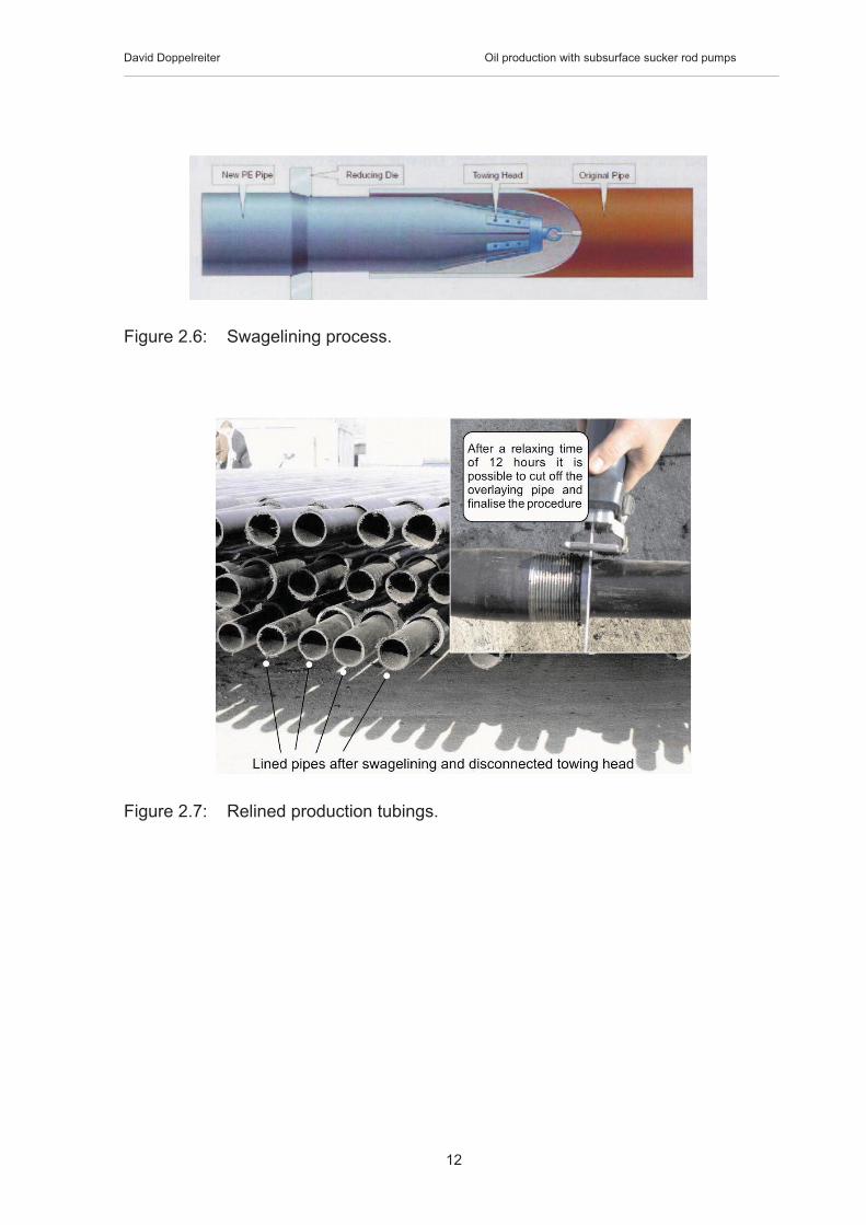
In general there are many kinds of technologies to reline tubings depending on different applications and dimensions. The common used technology for relining production tubings in the oil industry is called “Swagelining” (Figure 2.6). This manufacturing process was established by the British Gas (now Advantica) in the late 80’s.
The swagelining process uses pipes which have an outside diameter slightly larger than the inside diameter of the pipe to be lined. The first stages of the process are cleaning loose debris out of the host pipe and inserting a pull wire, which is then attached to a towing head on the plastic pipe. During the installation process, the pipe is pulled through a die to temporarily reduce the outside diameter. This reduction allows the pipe to be easily pulled through the host pipe by a winch. When the pulling force has been disconnected, the pipe begins to return toward its original diameter. However, just before the pipe relaxes completely it presses tightly against the inside of the host pipe, eliminating all annular space. Now it is possible to cut off the overlaying parts and finalise the relined pipe (Figure 2.7) [4].
David Doppelreiter Oil production with subsurface sucker rod pumps
12
Figure 2.6: Swagelining process.
Figure 2.7: Relined production tubings.

David Doppelreiter Oil production with subsurface sucker rod pumps
13
Figure 2.8: Relining process for OMV AG.
2.4 Tribology of polymer materials
2.4.1 What means tribology?
Tribology, which focuses on friction, wear and lubrication of interacting surfaces in relative motion (sliding, rolling, drilling, etc.) is a new field of science defined in 1967 by a committee of the organization for Economic Cooperation and Development [5]. The word “Tribology” is derived from the greek word “tribos” meaning rubbing, thus the literal translation would be the science of rubbing. It is only the name “Tribology“ that is relatively new, because interest in the constitute parts of tribology, like friction and wear, is older than recorded history [6]. The economical aspects of tribology are enormous in industrial states since the beginning of the 20th century. For this reason the knowledge in all areas of the tribology has expanded tremendously. Figure 2.9 shows a rough estimate (in billion

David Doppelreiter Oil production with subsurface sucker rod pumps
14
Figure 2.9: The various mechanical surface interaction phenomena included in the field of tribology [7].
of U.S. dollars) of the economic importance of each principal tribological topic, together with the amount of the gross national product of an industrial state that is dissipated in the various tribological processes. In United States the amounts dissipated added up to about $ 200 billion in 1985 - wear accounting three-quarters of the total [7]. In other words friction, wear and corrosion consume 4.5% of the gross national product of an industrial state [10]. Another usefull overview gives Figure 2.10. It represents the number of ways in which material objects lose their usefulness [7]. It is easy to see the importance of protecting objects from wear and corrosion because these are the main mechanism for material failures.
Figure 2.10: The causes of loss of usefulness of material objects with a percentage estimate of the economic importance of each [7].
David Doppelreiter Oil production with subsurface sucker rod pumps
15
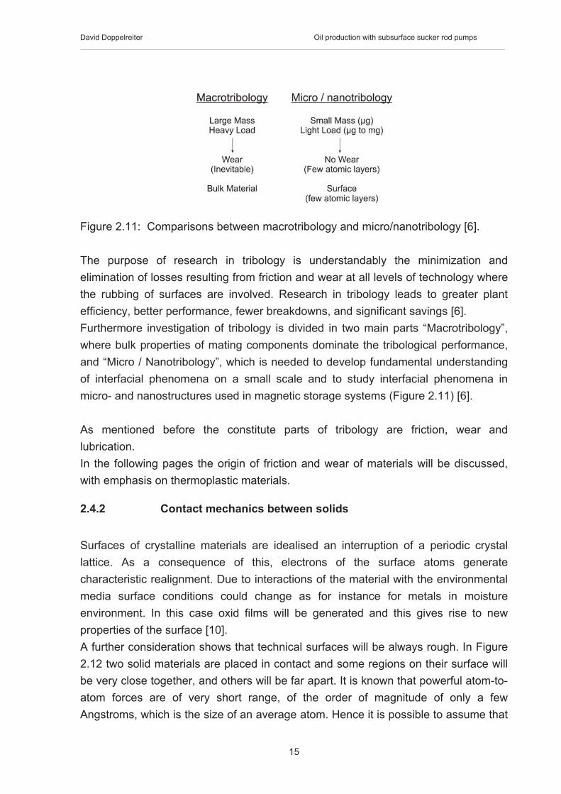
Figure 2.11: Comparisons between macrotribology and micro/nanotribology [6].
The purpose of research in tribology is understandably the minimization and elimination of losses resulting from friction and wear at all levels of technology where the rubbing of surfaces are involved. Research in tribology leads to greater plant efficiency, better performance, fewer breakdowns, and significant savings [6]. Furthermore investigation of tribology is divided in two main parts “Macrotribology”, where bulk properties of mating components dominate the tribological performance, and “Micro / Nanotribology”, which is needed to develop fundamental understanding of interfacial phenomena on a small scale and to study interfacial phenomena in micro- and nanostructures used in magnetic storage systems (Figure 2.11) [6].
As mentioned before the constitute parts of tribology are friction, wear and lubrication.In the following pages the origin of friction and wear of materials will be discussed, with emphasis on thermoplastic materials.
2.4.2 Contact mechanics between solids
Surfaces of crystalline materials are idealised an interruption of a periodic crystal lattice. As a consequence of this, electrons of the surface atoms generate characteristic realignment. Due to interactions of the material with the environmental media surface conditions could change as for instance for metals in moisture environment. In this case oxid films will be generated and this gives rise to new properties of the surface [10]. A further consideration shows that technical surfaces will be always rough. In Figure 2.12 two solid materials are placed in contact and some regions on their surface will be very close together, and others will be far apart. It is known that powerful atom-to-atom forces are of very short range, of the order of magnitude of only a few Angstroms, which is the size of an average atom. Hence it is possible to assume that

David Doppelreiter Oil production with subsurface sucker rod pumps
16
all the interaction take place at those regions between the surfaces at which there is atom-to-atom contact. These regions will be referred to as “junctions”, and the sum of the areas of all the junctions constitute the “real area” of contact Ar. The total interfacial area, consisting of both the real area of contact and those regions that appear as if contact might have been made there, will be denoted as the “apparent area” of contact Aa [7].
Figure 2.12: Schematic view of an interface, showing the apparent (Aa) and real (Ar)areas of contact
Size of the real area of contact
In view of the fact that the nature of the interaction between two surfaces is determined by the real area of contact, it is necessary to derive as much information as possible about the size of the real area [7].In the early studies of contacts between the real surfaces it was assumed that since the contact stresses between asperities are very high the asperities must deform plastically. This assumption was consistent with Amonton’s law of friction, which states that the friction force is proportional to the applied load, providing that this force is also proportional to the real contact area. However, later on it was shown that the contacting asperities, after an initial plastic deformation, attain a certain shape where the deformation is elastic. It has been demonstrated on a model surface made up of large irregularities approximated by spheres with a superimposed smaller set of spheres which where supporting an even smaller set (Figure 2.14), that the relationship between load and contact area is almost linear despite the contact being elastic. It was found that a nonlinear increase in area with load at an individual contact is compensated by the increasing number of contacts. A similar tendency was also found for real surfaces with random topography. It therefore became clear that Amonton’s law of friction is also consistent with elastic deformations taking place

David Doppelreiter Oil production with subsurface sucker rod pumps
17
at the asperities providing that the surface exhibits a complex hierarchical structure so that several scales of microcontact can occur [5].
Elastic Deformation (Hertzian theory, 1881)
The elastic contact deformation of spherical bodies is described by the theory of Hertz on condition of pure elastic materials, idealized flat surfaces and a static normal load. Moreover the bases of calculation for the contact cylinder-cylinder (line-contact) and ball-ball (point-contact) are assembled (Figure 2.13). Due to this a calculation of the basic magnitudes, like the nominal elastic contact area, the normal pressure distribution and the maximum surface pressure, in case of elastic contact deformation for line- and pointcontacts can be evaluated [10].
Figure 2.13: Bases of calculation for pure elastic contact deformation by Hertz [10]
This theory of highly idealized flat surfaces was advanced from Achard (1953) through the model of a rough surface approximated by a serious of hierarchically superimposed spherical asperities (Figure 2.14). Although this model is oversimplified too it shows that the real area of contact Ar is directly proportional to the normal load and given by

David Doppelreiter Oil production with subsurface sucker rod pumps
18
CN
r EFconstA ��
����� (Equ. 2.3)
FN: normal load E: reduced Young’s Modulus of the contact materials C: factor depends on the model 45/445/4 C
Furthermore mathematical analysis of Greenwood and Tripp showed that the number of microcontacts is approximately proportional to the normal load the real area of contact is proportional the number of microcontacts and
therefore proportional to the normal load; Ar = const. FN
the average size of a microcontact is not depending on the normal load. The basic for less wear are pure elastic deformed microcontacts. [10]
Figure 2.14: Contact between idealized rough surface approximated by a serious of hierarchically superimposed spherical asperities and a perfectly smooth surface [5]
Viscoelastic Deformation
For the contact of viscoelastic materials like polymers it is necessary to add rheological models to the elastic contact deformation. Bodies are called viscoelastic if they exhibit simultaneously time-independent elastic properties and time-dependent viscous properties. This behaviour can be modelled by two simple combinations of springs and dashpots. The connection of spring (Hookean body) and dashpot (Newtonian liquid) in series leads to the Maxwell element (for relaxations) and in parallel to the Voigt-Kelvin element (for retardations). Both models describe linear viscoelasticity since they combine stresses, deformations and deformation rates linearly. Additional combinations of springs and dashpots lead to more complicated elements, for example, the Burgers element (4-parameter element) as a Maxwell
1st order 2nd order
3rd order

David Doppelreiter Oil production with subsurface sucker rod pumps
19
element and a Voigt-Kelvin element in series as you can see in the following figure [11].
Figure 2.15: Viscoelastic deformation described by the Burger model [10].
The spring with the Young’s modulus E0 describes the pure elastic condition whereas the time-dependent viscoelastic component is described by the Voigt-Kelvin element due to a spring (relaxation modul Er) and a dashpot (viscosity �r). The relaxation time � indicates the time after which the stress is reduced to 36.8% of its original value. In addition to the viscoelastic element a viscoplastic component with the viscosity �o
can take effect too. For uniaxial stress 0 a total deformation �total = �l/l0 is given by the following parts and equations:
rveltot ���� ��� (Equ. 2.4)
elastic deformation 0
0
Eel � � (Equ. 2.5)
viscoelastic deformation
��
���
��
��
�t
r
r
E exp1
0 (Equ. 2.6)
viscoplastic deformation 0
0 *� � t
v � (Equ. 2.7)

David Doppelreiter Oil production with subsurface sucker rod pumps
20
Via an asymptote to the resulting �total curve the relaxation modul Er and the relaxation time can be determined. As a result of this the viscoelastic contact deformation of viscoelastic materials can be estimated (negligible viscoplasticity) by a summation of the elastic and viscoelastic components. Thereby the Young’s modulus E0 of the viscoelastic component would be displaced by a term including relaxationmodul Er and relaxation time �. The total contact deformation � for viscoelastic materials during load in a pointcontact (Figure 2.13) is shown by the following lines (Czicho, 1985) [10]:
�total = �el + �r (Equ. 2.8) �
�el … Hertzian theory (Figure 2.13)
�r … Hertzian theory with r
t
E
e
E
���
����
��
�
��1
1
0
3/2
3/1
2
2
3/23/1
2'0 16
19
169
Nr
t
Ntotal FRE
eF
RE�����
�
�
�����
�
����
����
��
���
���
��
��
� (Equ. 2.9)
2
22
1
21
'111EEE�� �
��
� (Equ. 2.10)
�1, �2: poisson ratio E1, E2: Young’s moduli R: ball radius E’: reduced Young’s modulus
Although these formulas are very simplified their approximations are really suitable [10].
Plastic Deformation
For the transition from elastic to plastic deformation different criterions were developed. The index of plasticity is given by Greenwood und Williams (1966):
2/1*'
* ���
����
����
����
��
� �
HE (Equ. 2.11)

David Doppelreiter Oil production with subsurface sucker rod pumps
21
E’: reduced Young’s modulus of the contact partners H: Hardness
�: standard deviation of the roughnesshill distribution �: average radius of the roughnesshills
As a result of this criteria the index of plasticity � < 0.6 describes an elastic and � > 1 a plastic contact deformation. Due to detailed analysis of the conditions and results of a plastic contact deformation similar conclusions like for the elastic contact deformation were established:
the real area of contact is proportional to the normal load FN
increasing normal load FN results in increasing real area of contact through an increase of the number of microcontacts. The average size of a microcontact is constant [10]
Contact mechanics between solids including adhesion
The previous handling of contact procedures dealed only with the pure contact mechanic based on the Hertzian theory. A special analysis of the elastic contact of spherical bodies with idealized flat surface and adhesion - characterised by the interface energy � - was made by Johnson, Kendall and Roberts (1971). This analysis showed that due to adhesion a release force is necessary, independent of the normal load, to disconnect the contact partners:
� !!��� rFN 23 (Equ. 2.12)
Figure 2.16: Hertzian contact between two spheres including adhesion [10]

David Doppelreiter Oil production with subsurface sucker rod pumps
22
Now the contact ranges, in consequence of adhesion, over a bigger area with compression stress in the middle and a tensile stress at the border. Fuller and Tabor (1975) showed that the influence of adhesion at the contact deformation is depending on the roughness. Magnitudes of surface roughness where adhesion more or less disappears are Ra ~ 1 µm for Van der Waals materials and Ra ~ 5 nm for hard materials [10].
Material effort for normal force load
The Hertzian theory is the basis for the calculation of the material effort by the contact of curved surfaces. In Figure 2.17 a the contact tensions, the maximum shear stresses as well as the comparison stresses of von Mises and Tresca are represented. The maximum of the comparison stresses of von Mises and Tresca are below the surface. The dependence of the material effort due to geometry (line- or pointcontact) is shown in Figure 2.17 b [10].
Figure 2.17: Material effort due to normal force load [10]
Material effort for normal- and tangential force load
Because of friction forces superposition of normal and tangential loads will occur. Due to this superposition, under otherwise similar conditions like before, an increase of the material effort and an asymmetry of the stress fields in the counterparts will appear. The gradient of the comparison stress in case of line-contact under pure normal force load (f=0) as well as for superimposed friction with friction factors of f=0.1, f=0.2 and f=0.3 is shown in Figure 2.18
a b

David Doppelreiter Oil production with subsurface sucker rod pumps
23
Figure 2.18 Standardised comparison stress for normal load (f=0) and for superimposed normal and tangential load (f=0.1; 0.2; 0.3) (line-contact cylinder/cylinder) [10]
Already for friction factors f=0.2 the comparison stress at the surface reaches the similar value of the comparison stress-maximum below the surface. In case of f=0.3 the comparison stress at the surface is considerable bigger as below the interface area. Similar to the yield criterion of von Mises and Tresca it is shown for pure normal load the plastic deformation is starting below the interface area whereas for superimposed tangential force through friction forces plastic deformation is moving to the surface. More influencing variables concerning tangential forces are temperature, kinematic, residual stresses, surface roughness and boundary layers [10].
2.4.3 Friction and wear of polymers
Polymers have some friction and wear properties that cannot be obtained by any group of materials. For example, the materials with minimum friction coefficients are polymers. In addition, the high chemical stability of many polymer molecules leads to a surface which is not considerably changed by reactions with the environment, such as oxidation. The differences between polymers and other materials originate primarily from the fact that, because of their particular molecular structure, a different set of physical properties dominates this system. These differences cannot be understood without some knowledge of the microstructure of polymeric materials, in particular of thermoplastic (semi-crystalline) polymers like polyethylene’s or polypropylene’s [12].

David Doppelreiter Oil production with subsurface sucker rod pumps
24
2.4.3.1 Classification of polymers
Polymers are divided into three parts, thermoplastics, elastomers and thermosets (Figure 2.19).The largest portions of polymers used in petroleum industry are thermoplastics. Thermoplastics consists of a crystalline and amorphous region and corresponds to different morphology, which will be discussed later on.Elastomers are crosslinked polymers, which can be stretched easily to high extensions and contract when the applied stress is released. Thermosets are rigid materials. These network polymers are restricted in chain motion, because of the high level of crosslinking.
Figure 2.19: Polymer classification
2.4.3.2 Structure and properties of thermoplastic materials
Polymer is a term used to describe large molecules consisting of repeating structural units, or monomers, connected by covalent chemical bonds. The term is derived from the Greek words: “polys” meaning “many”, and “meros” meaning “parts”. A key feature that distinguishes polymers from other molecules is the repetition of many identical, similar, or complementary molecular subunits in these chains. These subunits, the monomers, are small molecules of low to moderate molecular weight, and are linked to each other during a chemical reaction called polymerization [14]. Figure 2.20 shows the molecular subunit, monomer, C2H4 and the resulting polyethylene chain after polymerization.

David Doppelreiter Oil production with subsurface sucker rod pumps
25
Figure 2.20: (a) Ethene molecule C2H4 linked to each other during chemical reaction to a (b) polymer – polyethylene chain [14]
Figure 2.21: (a) coiled structure (L = average distance between chain ends) for amorphous materials (b) semi-crystalline structure (black points indicate the start and the end of the macromolecules) [12][15]
Influence of polymerization on thermoplastic materials
The degree of polymerization of a macromolecule denotes the number of monomeric units in a macromolecule. As mentioned above a polymer consists of many macromolecules which may or may not have the same degree of polymerization. If the polymer is non-uniform with respect to the degree of polymerization of its molecules, then it has a distribution of degrees of polymerization which can be described by a distribution function.Degrees of polymerization are important theoretical quantities. They cannot be measured directly and have to be calculated from experimentally determined molar masses M or molecular weights MW.The molecular weight MW is the mass of one molecule of that substance, relative to the unified atomic mass unit u (equal to 1/12 the mass of one atom of carbon-12).
a b
a b
David Doppelreiter Oil production with subsurface sucker rod pumps
26
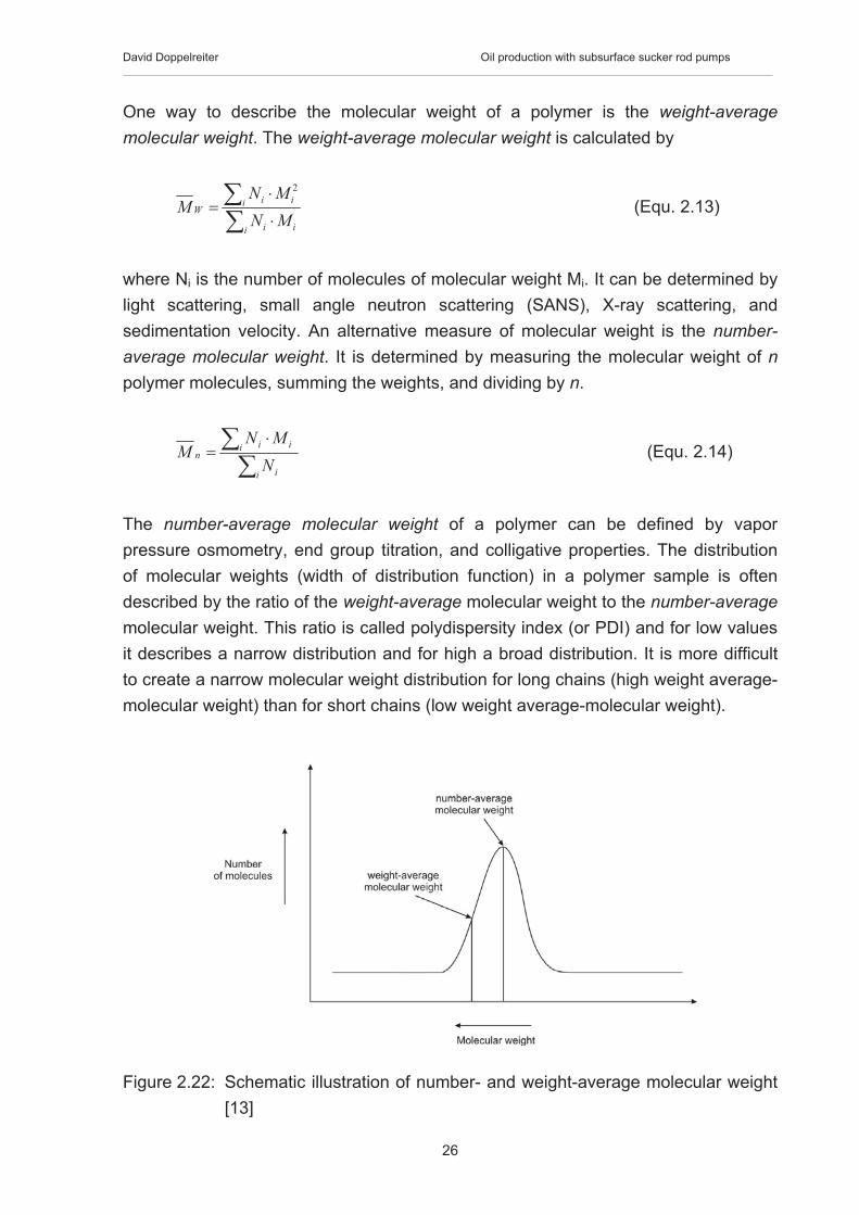
One way to describe the molecular weight of a polymer is the weight-average molecular weight. The weight-average molecular weight is calculated by
""
!
!�
i ii
i iiW
MNMN
M2
(Equ. 2.13)
where Ni is the number of molecules of molecular weight Mi. It can be determined by light scattering, small angle neutron scattering (SANS), X-ray scattering, and sedimentation velocity. An alternative measure of molecular weight is the number-average molecular weight. It is determined by measuring the molecular weight of npolymer molecules, summing the weights, and dividing by n.
"" !
�i i
i iin
NMN
M (Equ. 2.14)
The number-average molecular weight of a polymer can be defined by vapor pressure osmometry, end group titration, and colligative properties. The distribution of molecular weights (width of distribution function) in a polymer sample is often described by the ratio of the weight-average molecular weight to the number-averagemolecular weight. This ratio is called polydispersity index (or PDI) and for low values it describes a narrow distribution and for high a broad distribution. It is more difficult to create a narrow molecular weight distribution for long chains (high weight average-molecular weight) than for short chains (low weight average-molecular weight).
Figure 2.22: Schematic illustration of number- and weight-average molecular weight [13]

David Doppelreiter Oil production with subsurface sucker rod pumps
27
The molecular weight is influencing different properties of a thermoplastic polymer. Low molecular weight is resulting in:
� less strength � less rigidity � higher creeping during sustained loading � less wear resistance � less impact strength � worse form stability
The molecular weight distribution shows for broad distribution similar effects. High low-molecular rates will soften the material and an easy sliding of the polymer chains is possible. This is resulting in e.g. good processibility compared to worse longtime properties, however a narrow molecular weight distribution with high rates of high-molecular chains shows worse processibility but better mechanical longtime properties.The branching factor, with his great impact on crystallinity, is influenced by the polymerization too as well as the tactivity (see Figure 2.23, Figure 2.25) [11,15]. Low density polyethylene (PE-LD) materials show high branching factors in comparison to high density polyethylene (PE-HD) materials.
Table 2.1: Effect of molecular weight on thermal properties of PE
Number of CH2-CH2
units
MolecularWeight (MW)
Softeningtemperature
°C
Character of Polymer
at 25°C
1 30 -169 Gas 6 170 -12 Liquid 35 1000 37 Grease
140 4000 93 Wax 250 7000 98 Hard wax 430 12000 104 Plastic 750 21000 110 Plastic 1350 38000 112 Plastic

David Doppelreiter Oil production with subsurface sucker rod pumps
28
Figure 2.23: Schematic illustration of different branching factors of PE [15].
Molecular structure
Many aspects of the frictional behaviour of polymers are directly related to themolecular structure. Straight, stiff molecules must be distinguished from those which have the tendency to coil. Straight molecules are able to form crystals while coiled, branched molecules can only form glassy (amorphous) structures. Some chains form helices, as, for example, PTFE. Its large F-atoms cause great stiffness, which in turn leads to a high crystallinity, in spite of the weakness of the intermolecular bonds.
Thermoplastic materials are mixtures of crystalline and glassy regions. The elementary crystalline element is the folded lamella. These lamellae in turn are stacked into packages, surrounded and tied together by non-crystalline portions of the microstructure (Figure 2.21). Cohesion between molecules increases with degree of crystallization. Some of the special arrangements are the microcrystalline structure and the spherulitic structure (Figure 2.25 a,b). Cohesion of polyethylene (PE) is predominantly due to their high crystallinity, while their specific intermolecular bonds are relatively weak because of a symmetric molecule structure.The molecule itself can be symmetric or asymmetric, depending on the position of the side groups (Figure 2.24). A consequence of asymmetric shape of the molecule is the formation of net electric dipole moments, which in turn form the basis for strong intermolecular bonding. All strength thermoplastic polymers are characterized by the existence of strong dipoles (PVC, PE) or of still stronger hydrogen bonds (PA).

David Doppelreiter Oil production with subsurface sucker rod pumps
29
Figure 2.24: Molecular structure – influence of different types of intermolecular bonding on surface energy and cohesion [12]
Figure 2.25: (a) Fine crystalline PP quenched from 220°C to 20°C; (b) Coarse spherulitic PP, furnace cooled from 220°C to 130°C, 4h, quenched to 20°C; (c) Isotactic and atactic configuration of PP molecules [12]
Side groups can be arranged in a disordered or ordered way (tacticity) (Figure 2.25 c). High tacticity favors crystallisation. In symmetric molecules the dipole moments of the individual bonds compensate each other so that the bonds between individual molecules become relatively weak (see PE). This weakness of the intermolecular bond coincides with a low surface energy of the material. The strongest intermolecular bond is caused by cross-linking (covalent bonds linking one polymer chain to another), which is effective in thermosetting polymers, elastomers, and cements. The existence of this type of bond excludes the possibility of plastic deformation. The strength of unsaturated bonds in the surface will determine the surface energy. High cohesion between molecules is favored by high density of strong bonds.In an intermediate range of temperature and strain rate all thermoplastic materials can deform plastically, and, as a consequence, the molecules become aligned. During sliding, the maximum amount of deformation in the surface can surpass the one obtained in tensile test. The structure is then characterized by a high degree of molecular alignment in the direction of sliding. An important case is the coarse spherulitic structures in which small molecular-weight portions have been rejected during crystallisation, so that the boundary regions between the spherulites are
a b c

David Doppelreiter Oil production with subsurface sucker rod pumps
30
amorphous. The amount of the crystallinity and therefore cohesion is high inside the spherulites. [12] It has been theorized for some time that reducing the spherulite size of crystalline polymers should improve their wear resistance. The basic argument for this is that the size of wear particles produced is proportional to the spherulite size. Spherulites of crystalline material in a polymer are separated by layers of more brittle amorphous material. According to the model shown in (Figure 2.26), wear particles form by crack development between spherulites and their size is similar to that of the spherulites. [5]
Figure 2.26 Influence of the spherulite size on wear rate [5]
Bulk physical properties
The bulk properties of polymers are much different from those of metals in two respects. Mechanical properties vary over a wide range, from high elastic modulus and brittle behaviour at low temperatures through work hardening and relatively tough or rubber-elastic behaviour at intermediate temperature, to viscous behaviour at still higher temperatures. Low heat conductivity together with the low melting temperatures of most of the polymers leads to the particular sensitivity of all experimental results with respect to temperature, velocity of sliding, and load. This is one reason for a low degree of reproducibility of experimental results and the wide range of data found in the literature [12].

David Doppelreiter Oil production with subsurface sucker rod pumps
31
2.4.3.3 Thermoplastic materials
Polyethylene (PE)
Polyethylene is a semi-crystalline thermoplastic (2.4.3.1) commodity heavily used in consumer products. It is a polymer consisting of long chains of the monomer ethylene which is shown in Fehler! Verweisquelle konnte nicht gefunden werden..
Figure 2.27: Molecular structure of the monomer ethylene C2H4
Polyethylene is classified into several different categories based mostly on its density and branching. The mechanical properties of PE depend significantly on variables such as the extent and type of branching, the crystal structure, and the molecular weight.
� UHMWPE (ultra high molecular weight PE) is polyethylene with a molecular weight numbering in the millions, usually between 3.1 and 5.67. The high molecular weight results in less efficient packing of the chains into the crystal structure as evidenced by densities less than high density polyethylene. The high molecular weight results in a very tough material. Because of its outstanding toughness, cut, wear and excellent chemical resistance, UHMWPE is used in a wide diversity of applications.
� HDPE (high density PE) is defined by a density of greater or equal to 0.941 g/cc. HDPE has a low degree of branching (Figure 2.23) and thus stronger intermolecular forces and tensile strength.
� MDPE (medium density PE) is defined by a density range of 0.926 – 0.940 g/cc. MDPE shows better stress cracking resistance as well as less notch sensibility than HDPE.

David Doppelreiter Oil production with subsurface sucker rod pumps
32
� LDPE (low density PE) is defined by a density range of 0.910 – 0.940 g/cc. LDPE has a high degree of short and long chain branching (Figure 2.23), which means that the chains do not pack into the crystal structure as well. It has therefore less strong intermolecular forces and these result in a lower tensile strength but increased ductility. The high degree of branches with long chains gives molten LDPE unique and desirable flow properties.
� LLDPE (linear low density PE) is defined by a density range of 0.915 – 0.925 g/cc. It is substantially a linear polymer with significant numbers of short branches. LLDPE has higher tensile strength, higher impact and puncture resistance than LDPE.
� PEX is a medium- to high density polyethylene containing cross-linked bonds introduced into the polymer structure, changing the thermoplast into an elastomer. The high-temperature properties of the polymer are improved, its flow is reduced and its chemical resistance is enhanced.
Polypropylene (PP)
Polypropylene is as well as polyethylene a semi-crystalline thermoplastic material with an intermediate level of crystallinity between that of low density polyethylene (LDPE) and high density polyethylene (HDPE). Although the crystallinity is less than HDPE it is much more brittle and has a higher melting point. The crystallinity is strongly influenced by the tactivity of the molecular chain through the position of the CH3 groups. Fehler! Verweisquelle konnte nicht gefunden werden. shows the chemical structure of propylene.
Figure 2.28: Molecular structure of the monomer propylene C3H6.
The following table should give a small outline about the different properties of polyethylene and polypropylene.
David Doppelreiter Oil production with subsurface sucker rod pumps
33
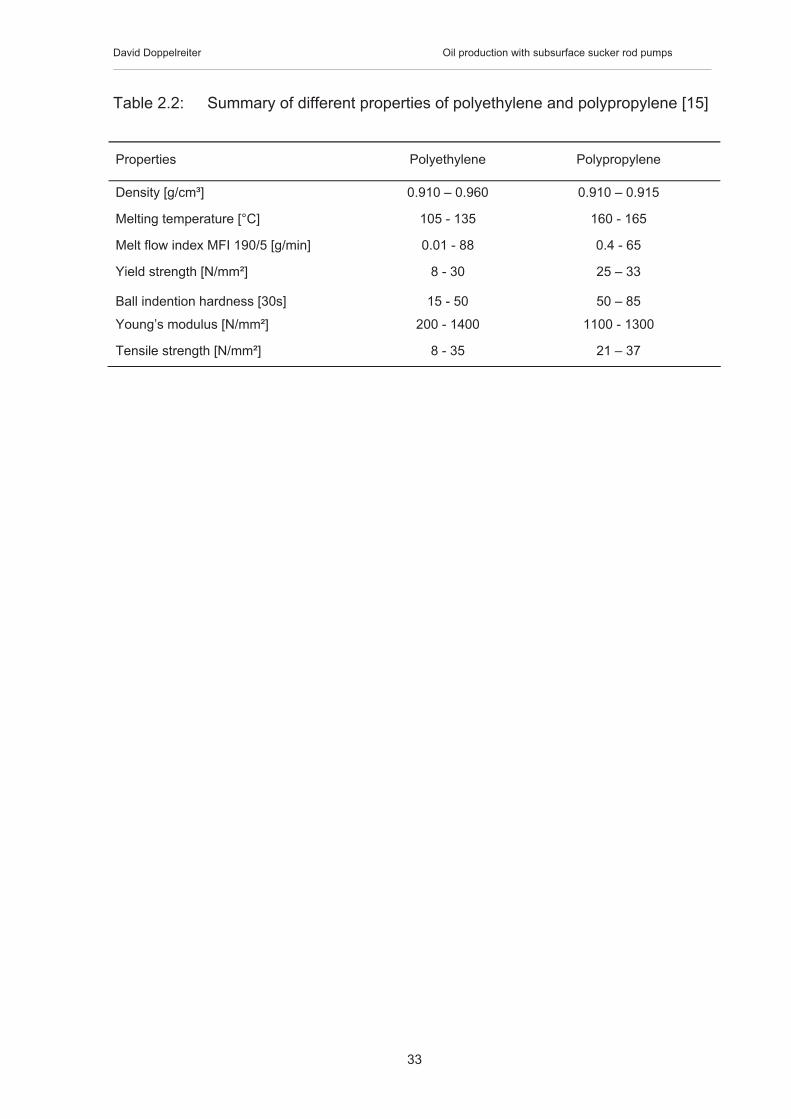
Table 2.2: Summary of different properties of polyethylene and polypropylene [15]
Properties Polyethylene Polypropylene
Density [g/cm³] 0.910 – 0.960 0.910 – 0.915
Melting temperature [°C] 105 - 135 160 - 165
Melt flow index MFI 190/5 [g/min] 0.01 - 88 0.4 - 65
Yield strength [N/mm²] 8 - 30 25 – 33
Ball indention hardness [30s] 15 - 50 50 – 85
Young’s modulus [N/mm²] 200 - 1400 1100 - 1300
Tensile strength [N/mm²] 8 - 35 21 – 37

David Doppelreiter Oil production with subsurface sucker rod pumps
34
2.4.3.4 Adhesion
It is evident in Table 2.3 that the surface energy, , of polymeric materials can vary over a wide range because of differences in molecular structure. The phenomenon of adhesion is due principally to the reaction of surfaces and the formation of interfaces in the real area of contact Ar. The change of the surface energy � is given by
dfadABBOAO *#�$��� (Equ. 2.15)
where AO, BO are the surface energies when the materials A, B have clean surfaces , AB is the surface energy of an AB interface (interfacial energy: required energy to enlarge the interface about 1m²), fad is the adhesion force per unit area and d is the intermolecular spacing. An attractive or a repulsive adhesion force can result:
dfad
�# (Equ. 2.16)
If two interfaces of like materials are brought into touch, an interface must form. It is identical with a kind of grain boundary containing only intermolecular bonds. For two different materials an intermolecular phase-boundary forms. The energy depends on the specific energies of the original surfaces and on that of the newly formed interface. If the interface is a “grain-boundary”, its energy, AA, is usually much smaller than that of the original surfaces, AO. For a given energy of the grain-boundary, AA, or interface, AB, the resulting adhesive force is small, if the original surface energies were small.
Table 2.3: Melting point, glass transition temperature, heat conductivity, and surface energy of several materials [12]

David Doppelreiter Oil production with subsurface sucker rod pumps
35
From the balance of specific energies several useful conclusions can be obtained for the adhesive forces which act between different combinations of materials:
fad is maximum, if similar materials with high surface energies are brought into contact or react. This is the case for high melting temperature materials, if their surfaces are not modified by reactions with their environment.
fad is minimum if two materials with low surface energies react and if these two materials produce an interface with high energy. Very low surface energies are found in polymeric materials with a symmetrical molecular structure such as PTFE and PE (see Table 2.3)
The interfacial energy AB increases with increasing difference in the nature of the bonding between two components A and B. Consequently, adhesion decreases in the following sequence: materials which form strong bonds �equal materials � different materials with mutual miscibility � materials which are not miscible but of similar type of bonding � materials of different type of bonding which are immiscible. Examples of the last-mentioned case are many combinations of metals and polymers in which little possibility for chemical bonding exists during sliding. Therefore combinations of PTFE or PE with steel, titanium and other alloys are frequently found [12].

David Doppelreiter Oil production with subsurface sucker rod pumps
36
2.4.3.5 Friction
Friction is originally the resistance against deformation. This means the power of resistance against material deformation at the beginning (static friction) and/or for the upkeep (dynamic friction) of a relative motion. In microscopic scale friction bases on processes which dissipate kinetic energy due to interactions between sliding bodies. Because of many different tribological conditions it is necessary to classify different types of friction:
Solid-Friction: friction between completely dry solids Dry-Friction: Friction with boundary layer Liquid-Friction: Counterparts are fully separated through a hydrostatic or
hydrodynamic liquid film Gas-Friction: Counterparts are fully separated through a aerostatic or
aerodynamic gaseous film Mixed-Friction: a parallel existence of Solid-Friction and Liquid- or Gas-Friction
Furthermore friction is a very complex act which should be appropriate an energy balance divided into the following terms:
Energy initiation � Contact between surfaces � Creation of the real area of contact
Energy transformation (Figure 2.29) � Adhesion processes � Deformation processes
Energy dissipation � Thermal processes � Energy absorption � Energy emission [10]
Friction mechanisms
Friction mechanisms are based on elementary processes (adhesion & deformation) in the real area of contact. After the results of the contact mechanic it is shown that the number of microcontacts increases approximately linear with the normal force. Every microcontact display an elementary motion resistance and therefore it is giving the following approach:
Friction force FR ~ number of microcontacts ~ normal force FN

David Doppelreiter Oil production with subsurface sucker rod pumps
37
The outcome of this is the friction law of Amonton-Coulomb (1699, 1785)
NR FF *%� (Equ. 2.17)
µ: Factor of proportionality
The Friction mechanisms could be arranged in the simplified illustration (Figure 2.29):
Figure 2.29: Simplified illustration of the basic friction mechanisms [10]
If friction is caused exclusively by adhesion and decohesion in the interface, the friction coefficient µ is defined as follows:
Nad
adNadR FHfAfFµF
ad*** ��� (Equ. 2.18)
However, decohesion of adhesive bonds is rarely the only contribution to friction. Only for low surface energies and very low compressive force, FN, is the frictional force determined by the adhesive tension, fad, and the effective asperity area, A. In this case A is reciprocally proportional to hardness for a certain range of forces.From this discussion it is evident that the coefficient of friction is determined by at least two materials properties – namely, the surface energy and the hardness. Figure 2.30 indicates the correlation between these two properties. For lower roughness the surface energy of the materials is determining the friction coefficient but in case of higher roughness the influence of adhesion due to the surface energies decreases and the friction coefficient is now determined by the hardness of each material. This statement applies to thermosetting materials which are not able to deform plastically,

David Doppelreiter Oil production with subsurface sucker rod pumps
38
and for which energy dissipated by elastic deformation can be neglected. When both adhesion (µad) and deformation (µdef) contribute to friction, the friction force is given by
NdefadNR FFF *)(* %%% ��� (Equ. 2.19)
Figure 2.30: Dependence of friction coefficient µ and roughness for a) elastic materials and b) less elastic materials [9]
In the case of thermoplastics, the frictional shear force which acts in the surface is usually higher than the critical shear stress needed to induce plastic deformation in the surface material. In this case deformation energy is dissipated and the surface is modified by molecular rearrangement. The molecules are aligned in the direction of sliding and considerable amounts of work hardening occur in this direction. In many cases the energy dissipated by plastic deformation will surpass far the energy used for decohesion of adhesive bonds in the surface. Consequently plastic deformation of the surface zone dominates the frictional force. This is always the case for abrasive friction, i.e. for hard particles plowing and cutting a surface. The change of surface structure, which causes work hardening, can lead to a decreasing coefficient of friction due to the increase of hardness and a decrease of the effective area. The effect of anisotropy of the surface energy may also contribute to the change of the friction coefficient with surface deformation. The surface energy should decrease slightly as a result of molecular realignment parallel to the surface. This effect is under investigation and is not yet completely clarified. The coefficient of friction increases with increasing surface energy of the polymeric material. Therefore it can be stated that, in contrast to metals in the atmosphere (shielding oxide layers), the coefficient of friction of the polymer is partly determined by its surface energy. As in metals it is also affected by the plastic deformation behaviour of the surface. In polymers oxidation of the surface plays a role in unsaturated molecular structures like those found in some elastomers. Large dipole moments will favour the tendency for formation of adhesive layers of water on the surface. Thus, shielding of the polymer surface can occur when high surface energy
a b

David Doppelreiter Oil production with subsurface sucker rod pumps
39
polymers are exposed to a humid environment. This effect is well known for PA and its relatively low friction coefficient is explained by the lubricating effect of its water layer.In addition to adhesive friction at asperities and mechanically activated plastic deformation with work hardening of the surface, a transition to viscous flow or melting occurs at higher temperatures. Before the transition to viscous flow a maximum coefficient of friction, which can lead to stick-slip behaviour, is sometimes found. This is due to surface softening, desorption of the water layer, and subsequent sticking of larger surface areas. It may be noted that the maximum of µ is most pronounced in materials of high surface energy (PA), while for low surface energy materials (PTFE, PE) the maximum, and therefore the tendency for stick-slip, is less pronounced or is absent.After the effect of surface energy and deformation behaviour on the coefficient of friction has been demonstrated, the question should be raised whether the original morphology of the polymer is important for friction. Mixtures of PP molecules of different tactivity may serve as the first example of such effects. Admixture of atactic molecules is associated with a reduced tendency for crystallisation and therefore reduced cohesion. The coefficient of friction increases with the portion of atactic molecules. This effect can be explained by the decreasing hardness of material containing higher portions of atactic molecules. The dependence of the coefficient of friction on morphology is qualitatively different if the polymer is rubbed against a material like steel which has different surface roughness. In the case of low surface roughness, a thin, highly deformed work-hardened layer can be form in the surface of the polymer. The amount of work hardening is more pronounced when the original hardness of the material is low. For the case of higher surface roughness this layer is removed by the abrasive wear more rapidly than it is re-formed. Therefore the original bulk mechanical properties (without surface work hardening) of the material become decisive for the coefficient of friction. This is an example of conditions for which the wear mechanism has a strong effect on friction. The maximum amount of deformation is limited by the surface fracture. In the case of brittle polymers the frictional force can induce cracking after small or negligible amounts of plastic deformation. In this case, only a limited amount of energy can be absorbed by plastic deformation before crack deformation occurs. Under these conditions a transition to a lower friction coefficient is expected which is partially determined by crack formation and crack extension energy. For polymers this situation can be achieved either at very low test temperatures (T << TG) or for mechanically heterogeneous materials. The latter case is demonstrated by the localized rupture of spherulite boundaries after negligible amount of deformation in

David Doppelreiter Oil production with subsurface sucker rod pumps
40
the interior of the spherulites themselves. The friction coefficient for this morphology is low, especially if hard spherulites are built from isotactic molecules which provide a high amount of crystallinity [12].
Adhesion component in sliding friction
The adhesion (2.4.3.4) component can be dropped down from values f ~ 0.1-0.6, under normal atmosphere and loads, to values smaller than f ~ 0.05 under conditions of mixed friction due to chemical active lubricants or rather to values f > 1 under ultra-high vacuum especially for sliding friction of metals.
Deformation component in sliding friction
The component of deformation is in particular high at the beginning of a relative motion between the counterparts and is characterized by the static friction coefficient (f ~ 0.4-0.75). The influence of the deformation component is getting weaker after levelling the original asperities (see Figure 2.31).
Crenation component in sliding friction
Normal values for the friction coefficient in the case of crenation are about f ~ 0.4. Higher values can be reached by a big penetration of wear debris and lower values will appear due to no wear debris in the interface between the two counterparts or if a very soft surface is rubbing against a hard and very smooth surface.
Figure 2.31 Schematic diagram of the run-in behaviour of pure thermoplastic materials [8]

David Doppelreiter Oil production with subsurface sucker rod pumps
41
Summarized it is to say that sliding friction under real conditions is always a superposition of the different friction components and therefore it is not possible to give any theoretical valuation. The determination of friction coefficients in a technical application is just possible through experimental readings [10].

David Doppelreiter Oil production with subsurface sucker rod pumps
42
2.4.3.6 Wear
Wear can be defined as the removal of material of a solid surface during relative motion. After the results of the contact mechanic (2.4.2) it is demonstrated that the real area of contact is approximately proportional to the normal load FN and furthermore the number of demands of micro contacts during sliding motion is increasing directly with the sliding distance. If every demands of the micro contacts results in wear debris the following approach is given:
Wear volume WV ~ normal load FN
Wear volume WV ~ sliding distance x Wear volume WV ~ wear factor k [mm³/Nm] by Archard
xFkW NV !!� (Equ. 2.20)
Wear is a result of elementary interactions between surfaces and these can be divided in the following parts:
� Interactions which are created by strength, stress or energy. These interactions lead to crack formation or extension and material separation of the contact partners and are characterized by the wear mechanisms “surface fatigue” and “abrasion”.
� Atomic and molecular interactions, which refer to chemical bondings in the contact area, are summarized by the wear mechanisms “adhesion”and “corrosive wear” [10].
Figure 2.32: Summary of wear mechanisms [10]

David Doppelreiter Oil production with subsurface sucker rod pumps
43
Surface fatigue
In many well lubricated contacts adhesion between two surfaces is negligible, yet there is still a significant rate of wear. This wear is caused by deformations sustained by the asperities and surface layers when the asperities of opposing surfaces make contact. Contacts between asperities accompanied by very high local stresses are repeated a large number of times in the course of sliding or rolling, and wear particles are generated by fatigue propagated cracks, hence the term “fatigue wear”. Wear under these conditions is determined by the mechanics of crack initiation, crack growth and fracture. If a crack cannot form at the surface it will form some distance below the surface where the stress field (Figure 2.18) is still sufficiently intense for significant crack growth [5].
Figure 2.33: Schematic illustration and an example of surface fatigue wear [5,10]
Abrasion
Abrasion appears if one of the counterparts is much harder and rougher than the other one or if hard debris are in the interface between two surfaces. Onto Figure 2.34 abrasion can be divided into 4 different sub-processes:
� Micro-ploughingCharacterized by a strong plastic deformation but without a material removal.
� Micro-chippingA chip is generated ahead an abrasive hard particle whose volume is equivalent to the wear chamfer.
� Micro-cracking

David Doppelreiter Oil production with subsurface sucker rod pumps
44
Occur above a critical force especially at brittle materials along the wear chamfer.
� Micro-fatigueIn consequence of repeated micro-ploughing demands on the surface material removal happen. This process is to assign to surface fatigue [10].
Figure 2.34: Schematic illustration of abrasion mechanisms. The ratio between micro-ploughing and micro-chipping can be described by the fab factor [10]
Adhesion
Most solids will adhere on contact with another solid to some extend provided certain conditions are satisfied. Adhesion between two objects casually placed together is not observed because intervening contaminant layers of oxygen, water and oil are generally present. Adhesion is also reduced with increasing surface roughness (see 2.4.2) or hardness of the contacting bodies. Actual observations of adhesion became possible after the development of high vacuum systems which allowed surfaces free of contaminants to be prepared. Adhesion and sliding experiments performed under high vacuum showed a totally different tribological behaviour of many common materials from that observed in open air.Adhesive wear is a very serious form of wear characterized by high wear rates and a large unstable friction coefficient.

David Doppelreiter Oil production with subsurface sucker rod pumps
45
Corrosive wear
Corrosive and oxidative wear occur in a wide variety of situations both lubricated and unlubricated. The fundamental cause of these forms of wear is a chemical reaction between the worn material and a corroding medium which can be either a chemical reagent, reactive lubricant or even air. Corrosive wear is a general term relating to any form of wear dependent on a chemical or corrosive process whereas oxidative wear refers to wear caused by atmospheric oxygen. Both these forms of wear share the surprising characteristic that a rapid wear rate is usually accompanied by a diminished coefficient of friction. This divergence of friction and wear is a very useful identifier of these wear processes [5].
Table 2.4 is summarising all the different wear problems as mentioned above.
Table 2.4 Models for the different wear mechanisms [10]
Surface fatigue component
Abrasioncomponent
Adhesioncomponent
Corrosive wear component
xFH
cW NV !!!!
�1
2��� xF
HW NV !!!
&!�
1tan2
xFH
KW NV !!!�1 x
vF
HdkW N
V !!!!
�²²'''(

David Doppelreiter Oil production with subsurface sucker rod pumps
46
Wear of polymers
A comparison of metals and polymers indicates that because of their very low hardness the wear rate of polymers is always higher than that of common materials. If different polymers are compared, it should be expected that for low friction forces acting in the surface, a low wear rate is the consequence. This is contradicted by the fact that the material with the lowest surface energy and lowest friction force; PTFE, shows the highest wear rate. The wear rate of PA, with its higher friction force, is much smaller. These observations indicate that for materials with low surface energy the strength of intermolecular bonds is so weak that separation is easy even by moderate friction forces. This antagonistic characteristic of friction and wear of polymers limits their application. It is a challenge to search for molecular structures and morphological effects by which both wear and friction can be minimized. This is, however, difficult to achieve, because weak intermolecular bonds are the prerequisites for a low surface energy, and therefore low friction. Strong bonds are required for high cohesion in the interior and high wear resistance. At the present stage of development one uses a species of molecules which form bonds that are relatively weak, because of its symmetrical molecular structure, but not too weak (PE). In HDPE a maximum bond density is achieved by crystallization, and entanglement is achieved by ultra-high molecular weights. An ideal material should have a structure with weak bonds acting through the surface and with strong ones in the interior. A material that preserves this structure while it is worn is not at present in sight. There is, however, a wide scope for improvements of the wear resistance by modifying molecules and molecular arrangements.
For very brittle materials the wear rate is controlled by the fracture toughness, while for ductile materials it is determined by the deformation processes preceding separation. There will be a transition for materials with an intermediate fracture toughness, for which maximum wear resistance can be expected. The transition point depends strongly on the wear system. The effect of fracture energy is mostly negligible for sliding on polished surfaces, while it becomes important for abrasion and for impact during erosion of polymers with low and even intermediate fracture toughness [12].

David Doppelreiter Oil production with subsurface sucker rod pumps
47
2.4.3.7 Abrasive Particles
Characterization and Classification of Abrasive Particles
Abrasive particles or grits are an inherent feature of many tribological systems. Two major factors controlling the abrasivity of a particle are its size and sharpness. It is intuitively felt that, in addition to hardness and size, particle shape plays an important role in abrasion. While it is relatively easy to quantify particle size, the numerical description of particle sharpness or angularity (sharpness describes the shape of the particle or surface protrusions in terms of its potential to abrade or erode) is much more difficult and determining the particle shape effects on abrasive wear rate is not an easy task. This is because wear depends on many different variables and the particle shape effect is often masked by stronger effects of other system variables. Particle shape in relation to abrasive or erosive wear is described by particle angularity or sharpness. Laboratory tests have confirmed that with the increase in the particle angularity there is a significant increase in abrasive or erosive wear rates. Work conducted on abrasive and erosive wear has demonstrated that any measure of particle abrasivity must include particle angularity.Traditionally, qualitative descriptors of particle visual appearance such as “spherical”, “semi-rounded”, “semi-angular” or “angular” have been used to classify and differentiate among various groups of abrasive particles. Typical shape parameters, often called shape factors, usually included in the image analysis software are the aspect ratio (width/length or sometimes length/width), roundness, form factor, convexity, elongation, etc. Shape factors have been developed for general particle description, without specific considerations relevant to the particle abrasivity. They describe the tendency of a particle to deviate from an ideal shape of a sphere. However, these parameters do not provide satisfactory information about the particle angularity since they do not indicate how sharp the particle protrusions or asperities are. So it has been quickly realized that abrasive particles require numerical descriptors that include the measure of sharpness (or angularity) of particle protrusions.
The ability of an abrasive particle to abrade depends strongly on its orientation to the wearing surface (or angle of attack). For example, an elongated particle with sharp ends oriented along its longer axis to the wearing surface will not cause much damage. The situation will change when this longer axis is perpendicular to the wearing surface. Thus, a new technique (CFA – Cone Fit Analysis) involving angularity measurement at every orientation of the particle projection and over a

David Doppelreiter Oil production with subsurface sucker rod pumps
48
large range of penetration depth has been developed. In this way, the statistical description of particle sharpness as a function of penetration depth is obtained. As the particle abrasiveness depends on the portion of the particle forced to penetrate and abrade the wearing surface, the severity of abrasion depends on particle orientation. Based on this notion, very abrasive particles might be represented by cones with a large angle of attack, while mildly abrasive particles may be represented by cones with a small angle of attack.The classical abrasion model is schematically illustrated in Figure 2.35, where a single cone-shaped asperity with an angle of attack & is pushed against and abrades a flat surface. Two areas shown in Figure 2.35 are of interest to CFA: the projected penetration area ) and the groove area A. The projected penetration area ) is defined as the intersection of the cone with the theoretically planar wear surface, while the groove area A is the orthogonal projection of the cone in the traversal direction. According to this model, the wear volume V is proportional to load P, sliding distance L and the tangent of the attack angle &, and inversely proportional to hardness H. The analysis of abrasive particles by CFA involves using a specially developed computer program to calculate ) and A areas for cones fitted to digitized particle profiles. The effect of particle orientation is included in the calculation.
Figure 2.35: Schematic illustration of the projected penetration area ) and groove Area A concept [16]
The average groove area AAV calculated for all orientations is then plotted against the penetration area (load) resulting in the CFA curve (also called the groove function). The gradient of the groove function (defined in CFA as an angularity ratio *���+�,�)) is related to the abrasivity of the particles tested. Linear character of the CFA curve indicates that particle protrusions behave like cones. For most particle types, the

David Doppelreiter Oil production with subsurface sucker rod pumps
49
gradient of the CFA curve increases with increasing penetration depth, suggesting that the wear rate should also exhibit a rise with increasing load or decreasing hardness. CFA curves of six types of real abrasives are shown in Figure 2.36. The gradient of the curves indicates that glass beads are the least abrasive (the lowest gradient) and crushed alumina is the most abrasive (the highest gradient). However, the non-linearity of the curves shown in Figure 2.36 a suggests that the real particle protrusions differ in shape from a perfect cone.
Figure 2.36: a) CFA curves for typical abrasive grits. The grits were sieved to 150-300 µm size range b) Relationship between two-body abrasive wear rate and the average angularity ratio *AV of abrasives calculated by CFA [16]
The average angularity ratio *AV can then be used to find an average value of the asperity angle of attack:
)(tan 1 *AVP !�& � (Equ. 2.21)
It can be seen from Figure 2.36 b that the average angularity ratio calculated correlates well with the experimental two-body abrasion wear data. Despite the apparent progress, it had been realized that the CFA must suffer some inaccuracy due to the inadequate approximation of asperity shapes by cones, as real particle asperities are generally not conical. A modified technique, called sharpness analysis, was subsequently developed. This technique is more accurate as it uses the full integration of the particle boundary to determine the groove area and provides more detailed consideration of the averaging process and statistical variability of
a b

David Doppelreiter Oil production with subsurface sucker rod pumps
50
shape and size. The sharpness * is defined again as the ratio of the groove area A to the projected area ) as schematically illustrated in Figure 2.37. As natural particles may exhibit vastly different sharpness, depending on the penetration depth and orientation, the concept of average sharpness has been incorporated in the SA technique [16].
Figure 2.37: Schematic illustration of the sharpness * concept for conical (CFA) and realistic asperities (SA) [16]
Particle Size Effect in Abrasive Wear
It is generally accepted that the particle size effect begins to manifest itself at particle sizes below 100 µm.
Figure 2.38: Effect of particle size on wear rate in two-body abrasion. Quartz particles, average of two tests plotted, 200 mm/s sliding speed, 9 mm (diameter) chalk pin. [16]

David Doppelreiter Oil production with subsurface sucker rod pumps
51
This trend can be observed in Figure 2.38 where the wear rates of chalk begin to decline when the quartz particle sizes drop below 150 µm for all three loads used in testing.The interpretation of the apparent reduction in wear rate with the decreasing particle size is far from consistent. Some authors attribute this to the increased particle roundness with decreased particle size, while other suggest a material strengthening mechanism, often called the “strain gradient effect”, at reduced scales. Similar strengthening is observed in micro- and nanoindentation tests. This effect can be observed at indentation diameters below 50 µm. With the reduction in indentation size down to 1 µm, the strength of the material, defined as the ratio of force to indentation area, can double or even triple. The argument that the smaller particles are more rounded is often not supported by microscopic examination of real particles. It was found, e.g. for quartz particles ranging in size from 40 to 250 µm, that it is virtually impossible to notice any increase in roundness with decreasing size of particles.In real contacts between two – body abrasive wear only a small number of the most exposed asperity peaks support load. Large valleys remain between the contacting asperity points and, under low loads, they can act as a reservoir for debris accumulation. The wear debris clogging the valleys can play a substantial role in separating the surfaces, and mitigating wear. This becomes more likely as the particle size decreases. However, for the clogging theory to be plausible for the explanation of the particle size effect a stronger relationship between the load, material hardness and wear rate would be expected but this is not the case. It is possible that with increased load and asperity penetration, debris are more effectively cleared into the surface valleys. As it would be expected, increasing load produces more debris but at the same time it compresses them. The wear debris are then pushed out of the way during the abrasive contact. The combination of these effects may explain why the critical particle size effect is not more strongly pronounced with increasing load as illustrated in Figure 2.38 [16]. Deterioration of abrasive grits as the cause of wear rate decrease is proposed in another work [17]. It is argued that smaller particles endure abrasive contact for a relatively greater displacement and are therefore more prone to deterioration. It seems that the end effect of particle attrition is similar to the effect of clogging. Considering all the evidence presented above, it appears that a combination of various mechanisms may contribute to the particle size effect, i.e. clogging/deterioration mechanisms and the scale-dependent strengthening of the abraded material [16].

David Doppelreiter Experimental
52
3 Experimental Operation
3.1 Materials
For describing the wear behaviour of polymer materials against different counterparts like couplings and rod centralizers two different polyolefin materials of different molecular structures were tested against two different species of couplings (unalloyed steel coupling, spray metal coupling) and one kind of polyamide rod centralizer.
3.1.1 Polymers for lining
As mentioned before two different types of “mass polymers” were tested concerning their wear behaviour. These two types of polyolefin were polyethylene (PE) and polypropylene (PP) samples of different molecular structures. The reason for testing polyolefin materials is based on their low price, easy production and their good friction and wear behaviour. Because of these arguments polyolefin materials are consequently of big interest for the new technology of relined production tubing.The following table should give a short illustration of the price range of several polymer materials.
Table 3.1: Price area per kilogram polymer granulate in € (2003) [15]
Polymer Euro €
PE 0.50 - 1.75
PP 0.50 – 2.50
PS 0.85 - 1.30
PVC 0.55 - 1.40
PA 6 2.50 - 6.00
PA 6.6 3.00 - 6.50
PA 11 7.50 - 11.50
PTFE ca. 12.50
PEEK ca. 60.00

David Doppelreiter Experimental
53
Tested types of HDPE
Most of the polyolefin products derived from Borealis except 3 types. Hostalen CRP 100 (HDPE) originates from Basell, DiscroPlex PE 3408 (HDPE) and one type of polypropylene stem from Chevron Phillips Chemical Company.
Borstar® HE 3490-LS: It is a black, bimodal (against each other displaced molecular weight dispersion curves), high density polyethylene classified as a MRS 10.0 material (PE 100). Dispersed carbon black gives outstanding UV resistance. Long term stability is ensured by stabilisation system. (Company: Borealis)
Borstar® HE 3493-LS: It is a natural, bimodal, high density polyethylene classified as a MRS 10.0 material (PE 100). It is just deviating from HE 3490-LS due to the absence of dispersed carbon. (Company: Borealis)
Bostar® HE 3470-LS: It is a black, bimodal, high density polyethylene classified as a MRS 8.0 (PE 80). Dispersed carbon black gives outstanding UV resistance. Long term stability is ensured by stabilisation system. (Company: Borealis)
BoarcoatTM HE 3450: It is a black high density polyethylene. It contains fine dispersed carbon particles to ensure weathering resistance. It is recommended as top coat in steel pipe coating. (Company: Borealis)
Hostalen® CRP 100: It is a black high density polyethylene with high melt viscosity for extrusion, injection and compression moulding. The product is classified as PE 100 and provides excellent stress cracking resistance properties combined with a very good long term hydrostatic strength. (Company: Basell)
DriscoPlex® PE 3408: Western Falcon black pipe; Black coloured high density polyethylene. (Company: Chevron Phillips Chemical Company)

David Doppelreiter Experimental
54
MG 9641: High Density Polyethylene for injection moulding. applications include crates, trays, boxes and housewares where good rigidity and impact strength is required. (Company: Borealis)
Material 17: Prototype - natural high density polyethylene not used for sale yet. (Company: Borealis)
Table 3.2: General properties of high density polyethylenes [18]
PolymerDensity '�[kg/m³]
weight average-molecular weight
Mw [g/mol]
number average-molecular weight
Mn [g/mol]
MFR*[g/10min]
Hardness [Shore]
Yieldstrength** [N/mm²]
HE 3490-LS 950 329000 6714 0.25 65 23.3
HE 3493-LS 950 330000 7000 not available 64 23.66
HE-3470-LS 946 329000 6714 0.3 64 20.23
HE 3450 942 not available not available 2 62 16.99
CRP 100 959 not available not available 0.2 60 19.43
PE 3408 Western Falcon
Black Pipe 955 not available not available not available 64 18.89
MG 9641 964 not available not available not available 63 22.65
Material 17 952 370000 10000 2.5 65 21.12
*Melt flow rate (190°C / 5kg) **(50 mm/min)

David Doppelreiter Experimental
55
Tested types of MDPE
Bostar® ME 3440-01: Black coloured, bimodal medium density polyethylene classified as a MRS 8.0 (PE 80). (Company: Borealis)
Table 3.3: General properties of medium density polyethylene [18]
PolymerDensity '�[kg/m³]
weight average-molecular weight
Mw [g/mol]
number average-molecular weight
Mn [g/mol]
MFR*[g/10min]
Hardness [Shore]
Yieldstrength **
[N/mm²]
ME 3440-01 951 329000 6714 0.85 65 17.53
*Melt flow rate (190°C / 5kg) **(50 mm/min)
Tested types of LLDPE
BoreceneTM FM 5270: Unimodal, metallocene low density polyethylene grade intended for production of packaging film. It has excellent optical properties in combination with good stiffness. (Company: Borealis)
BoreceneTM FM 5220: Unimodal, metallocene low density polyethylene grade intended for production of packaging film. It has excellent optical properties in combination with great puncture resistance and sealing strength. (Company: Borealis)
FG 5190: Butene based LLDPE grade intended for production of packaging film with high puncture resistance and strength. (Company: Borealis)
Material 4: Prototype – natural linear low density polyethylene not used for sale yet. (Company: Borealis)

David Doppelreiter Experimental
56
Table 3.4: General properties of linear low density polyethylenes [18]
PolymerDensity '�[kg/m³]
weight average-molecular weight
Mw [g/mol]
number average-molecular weight
Mn [g/mol]
MFR*[g/10min]
Hardness [Shore]
Yieldstrength **
[N/mm²]
FM 5270 927 144000 46452 1.3 55 11.70
FM 5220 922 162000 55862 1.3 55 10.16
FG 5190 919 133000 29556 1.2 53 8.58
Material 4 934 140000 46000 1.2 58 13.86
*Melt flow rate (190°C / 2.16kg) **(50 mm/min)
Tested types of PP
BA 202 E: It is a high melt strength polypropylene block copolymer for foam extrusion, to be used in addition with a foaming agent. It is recommended as thermal insulation for steel pipe coating in offshore applications. (Company: Borealis)
BorECOTM BA 212 E: It is a high molecular weight, low melt flow rate polypropylene block copolymer with very high stiffness and impact strength. It is recommend for solid wall and structured wall non-pressure pipes fittings and chambers, thin-walled corrugated pipes and profiles. (Company: Borealis)
BorECOTM BA 222 E: It is a high molecular weight, low melt flow rate polypropylene block copolymer with superior stiffness and excellent impact strength. It is a PP-HM (polypropylene high modulus) material. It is recommended for solid wall non-pressure piping especially in underground drainage and sewerage and soil and waste applications. (Company: Borealis)
RA 130 E – 8427: It is a grey, high molecular weight, low melt flow rate polypropylene random copolymer compound with good flexibility. It is recommended for house hot and cold water
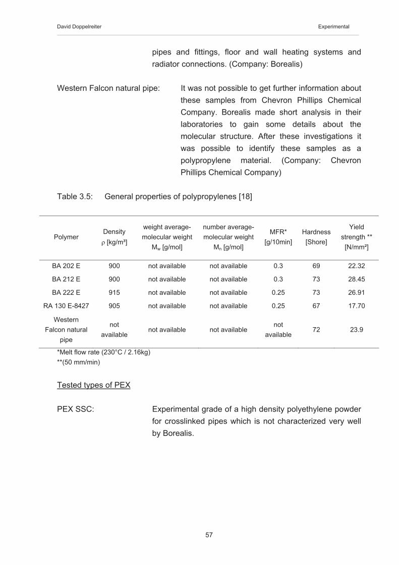
David Doppelreiter Experimental
57
pipes and fittings, floor and wall heating systems and radiator connections. (Company: Borealis)
Western Falcon natural pipe: It was not possible to get further information about these samples from Chevron Phillips Chemical Company. Borealis made short analysis in their laboratories to gain some details about the molecular structure. After these investigations it was possible to identify these samples as a polypropylene material. (Company: Chevron Phillips Chemical Company)
Table 3.5: General properties of polypropylenes [18]
PolymerDensity '�[kg/m³]
weight average-molecular weight
Mw [g/mol]
number average-molecular weight
Mn [g/mol]
MFR*[g/10min]
Hardness [Shore]
Yieldstrength **
[N/mm²]
BA 202 E 900 not available not available 0.3 69 22.32
BA 212 E 900 not available not available 0.3 73 28.45
BA 222 E 915 not available not available 0.25 73 26.91
RA 130 E-8427 905 not available not available 0.25 67 17.70
Western Falcon natural
pipe
notavailable
not available not available not
available72 23.9
*Melt flow rate (230°C / 2.16kg) **(50 mm/min)
Tested types of PEX
PEX SSC: Experimental grade of a high density polyethylene powder for crosslinked pipes which is not characterized very well by Borealis.

David Doppelreiter Experimental
58
Table 3.6: General properties of PEX [18]
PolymerDensity '�[kg/m³]
weight average-molecular weight
Mw [g/mol]
number average-molecular weight
Mn [g/mol]
MFR*[g/10min]
Hardness [Shore]
Yieldstrength **
[N/mm²]
PEX SSC 946 254000 87000 not
available61 20.74
**(50 mm/min)
3.1.2 Couplings
Two different types of couplings were used in the abrasion tests:
� Unalloyed steel couplings (Class T) and � Spray metal couplings (Class SM).
The goals of this study were the characterization of the wear behaviour of different polymers under sliding contact with spray metal couplings (Figure 3.1). A previous diploma thesis [19] had the emphasis to characterise the wear behaviour of polymer materials under contact with unalloyed steel couplings (Figure 3.1) and therefore it was necessary during this work to test the pairing polymer/unalloyed steel coupling if completely new materials had to be analysed.
Unalloyed steel coupling
The following table illustrates some specification details about unalloyed steel couplings.
Table 3.7: Specification of unalloyed steel couplings [20]
Tensile strength [MPa] max Sulphur content [%] Hardness [HRA] Roughness Ra [µm]
min. 655 0.05 56 - 62 < 3.125

David Doppelreiter Experimental
59
Spray metal coupling (Class SM)
Thermal sprayed metal coatings are depositions of metal which has been melted immediately prior to projection onto the substrate. The metals and application systems used vary but most applications result in thin coatings applied to surfaces requiring improvement to their corrosion or abrasion resistance properties [21].
Table 3.8: Specification of spray metal couplings [20]
Tensile strength [MPa]
max. Sulphur content [%]
SubstrateMaterial
Hardness [HRA]
Coating Hardness
[HV200]
Thickness of the coating
[mm]
Roughness Ra
[µm]
min. 655 0.05 56 - 62 min. 595 0.254 – 0.508 < 1.575
Figure 3.1: Illustration of an unalloyed steel- and spray metal coupling. These couplings are used in sucker rod pumps by OMV. Although the specification allows a surface roughness for spray metal couplings till ~1.6µm, OMV is using polished types with a roughness of ~ 0.1µm.

David Doppelreiter Experimental
60
3.1.3 Rod centralizer
Only one type of rod centralizer (polyamide) is used in sucker rod pumps by the OMV and therefore just this kind was tested. Chapter 2.1 gives a general description about rod centralizers and Figure 2.4 illustrates such a type. It was not possible to get much more information about the technical specification so
Table 3.9 will just give a basic outline about the properties of polyamide materials. Teflon is mixed into the polyamide matrix for reducing frictional forces.
Table 3.9: General properties of polyamide materials
PolymerDensity��'�[kg/m³]
weight average-molecular weight
Mw [g/mol]
number average-molecular weight
Mn [g/mol]
MFR*[g/10min]
Hardness [Shore]
Yieldstrength [N/mm²]
PA 6 1130 not available not available not
available74 40

David Doppelreiter Experimental
61
3.2 The pilot plant
The test facility simulates a translative movement of the sucker rod coupling or rod centralizer against the polymer lined tubing string under real conditions. For shortening the experimental time it is convenient to change the movement from translative to rotation by higher rotation speeds. Figure 3.2 shows the pilot plant from different perspectives.
Figure 3.2: Different pictures of the pilot plant in the OMV laboratory.

David Doppelreiter Experimental
62
For simulating the movement (rotation) two box column drills with variable rotation speed are used. These drilling machines are installed in basin 1 (made of aluminium) which is filled with the testing fluid. The polymer test samples are fixed on the stainless steel plates which are in connection with the power drill. Due to immiscibility of water and oil a circulating pump is standing in basin 1 for mixing the fluid during the whole testing procedure. Because of simulating real conditions it is necessary to keep a constant temperature (50°C) of the fluid and therefore a heating element is installed. Because of evaporation it is necessary to cover basin 1 with caps to reduce the loss of fluid and thus to keep a constant ratio between water / oil / salt / (sand). For reducing stench an extractor hood is directly placed above the pilot plant. The introduction of sand particles in the oil / water / salt mixture to simulate all real conditions made a modification of the pilot plant necessary. Due to centrifugal forces of the rotating plates it is not possible to place the sand particles between the couplings (or centralizer) and polymer plates. To solve this problem small metal pipes are installed (connected with the circulating pump) which inject the mixed medium directly under the centre of the polymer plates (Figure 3.3). After testing the fluid need to be filled in basin 2 and from this bin the water / oil / salt / (sand) mixture is pumped to a waste oil container.
Figure 3.3: Installed metal pipes for injecting sand-fluid mixture.

David Doppelreiter Experimental
63
3.3 Testing procedure
Due to the formation of different corrosion and abrasion products during a previous testing procedure it is essential to clean the whole pilot plant to get equal conditions for the next test run.Afterwards it is necessary to modify the polymer samples which arrive as quadratic plates from Borealis. For modifying the samples they are cut via jigsaw into round layouts. These modified plates are fixed through two metal rings (inner and outer ring) to the steel plate.Now two couplings (or centralizer) are placed at the bottom of each box column drill and are tightened quite strong so they cannot loose up during testing operation.Next step is the correct adjustment of the height of each drilling machine (see Figure 3.2; 5) and the mounting of both levers with the right lead weights.Finally basin 1 is filled with the raw oil / water / salt / (sand) mixture and the circulating pump is started to intersperse the medium. The heating element is activated and if good dissolving and right temperature is given the box column drills can be started.
3.4 Testing parameters
In field operations the stroke rate of a sucker rod pump is approximately 8 times per minute (depends on the inflow rate of the medium to pump). That means the coupling (or centralizer) passes the same place of the tubing 16 times per minute.The box column drill is set by a rotation speed of 345 rpm and a running time of 5 days and 21 hours. This testing procedure should simulate 127 days in field. For testing the counterpart polymer / unalloyed steel coupling or polymer / centralizer a force of 65 kg is loaded (separated on two couplings or centralizer) which comply a well deviation of 7° in field. In case of polymer / spray metal coupling the load is doubled.A fluid temperature of 50°C is kept and controlled by a heating unit to simulate equivalent conditions as you can find it in existing oil wells. The following tables show in detail the ratio of ingredients of the medium which is containing water, oil, salt and sand (sand was not used in all tests).
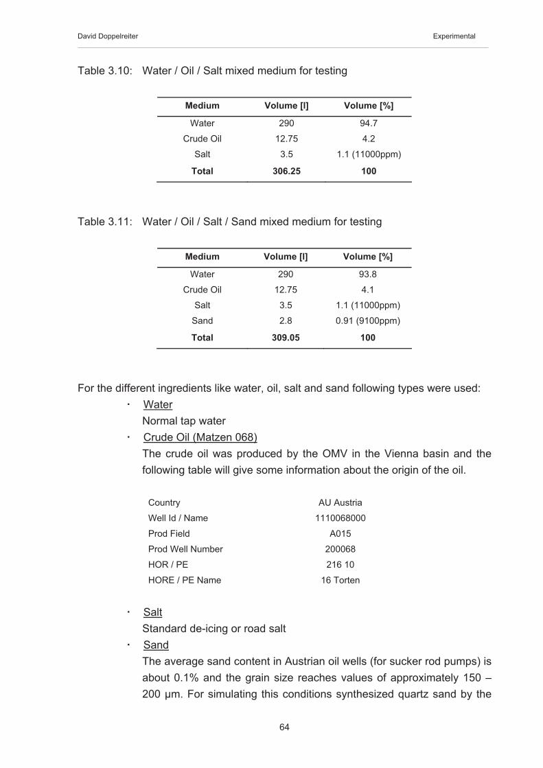
David Doppelreiter Experimental
64
Table 3.10: Water / Oil / Salt mixed medium for testing
Medium Volume [l] Volume [%]
Water 290 94.7
Crude Oil 12.75 4.2
Salt 3.5 1.1 (11000ppm)
Total 306.25 100
Table 3.11: Water / Oil / Salt / Sand mixed medium for testing
Medium Volume [l] Volume [%]
Water 290 93.8
Crude Oil 12.75 4.1
Salt 3.5 1.1 (11000ppm)
Sand 2.8 0.91 (9100ppm)
Total 309.05 100
For the different ingredients like water, oil, salt and sand following types were used: � Water
Normal tap water � Crude Oil (Matzen 068)
The crude oil was produced by the OMV in the Vienna basin and the following table will give some information about the origin of the oil.
Country AU Austria
Well Id / Name 1110068000
Prod Field A015
Prod Well Number 200068
HOR / PE 216 10
HORE / PE Name 16 Torten
� Salt Standard de-icing or road salt
� Sand The average sand content in Austrian oil wells (for sucker rod pumps) is about 0.1% and the grain size reaches values of approximately 150 – 200 µm. For simulating this conditions synthesized quartz sand by the

David Doppelreiter Experimental
65
company “Quarzwerke Österreich” was used for the testing procedure. Following data, like average grain size and the chemical composition of the quartz grains, were determined by the OMV laboratory (see appendix A)
3.5 Evaluation of materials and specimens
3.5.1 Shore D Durometer
A Durometer is one of several ways to indicate the hardness of a material, defined as the material's resistance to permanent indentation. It is measuring, like many other hardness tests, the depth of an indentation in the material created by a given force on a standardized presser foot. This depth is dependent on the hardness of the material, its viscoelastic properties, the shape of the presser foot, and the duration of the test. Shore durometer allows for a measurement of the initial indentation, or the indentation after a given period of time. The basic test requires applying the force in a consistent manner, without shock, for 15 seconds, and measuring the depth of the indentation. There are several scales of durometer, used for materials with different properties. The two most common scales, using slightly different measurement systems, are the A and D scales (Figure 3.4). The A scale is for softer plastics, while the D scale is for harder ones.
Durometer Indenting foot Applied force (g)
Type A Hardened steel rod 1.1 mm – 1.4 mm dia, with a truncated
35° cone, 0.79 mm dia 822
Type D Hardened steel rod 1.1 mm – 1.4 mm dia, with a 30°
conical point, 0.1 mm radius tip 4550
These tests are a useful measure of relative resistance to indentation of various grades of polymers. However, the Shore Durometer hardness test does not serve well as a predictor of other properties such as strength or resistance to scratches, abrasion, or wear, and should not be used alone for product design specifications. The correlation between Shore hardness and flexibility holds for similar materials, especially within a series of grades from the same product line, but this is an empirical and not a fundamental relationship [22].

David Doppelreiter Experimental
66
Figure 3.4: Correlation between two Shore Durometer hardness scales [22]
3.5.2 Chromatic coding confocal sensor
After testing the polymer surface (wear track) was analyzed by a special apparatus called MicroProf®. For determining the surface contours white light is scanning the top of the sample and an internal passive optic, using chromatic aberration, splits the white light into different colours (corresponding to different wavelengths). A miniaturized spectrometer detects the colour of the light reflected by the sample and determines the position of the focus point (Figure 3.5). By an internal calibration table the vertical position is measured on the sample surface.
Figure 3.5: Measuring principle of a chromatic sensor [23]
For measuring the tested polymer sample it is necessary to divide the plate into 4 equal pieces. Afterwards each of these pieces are put on the x-y table of the

David Doppelreiter Experimental
67
MicroProf® and a measurement normal to the wear track is done by white light (one-dimensional in x-direction). The units of the diagram axes are 9.91821*10-8 m (z-scale) and 8*10-2 m (x-scale).
Figure 3.6: MicroProf® apparatus for analysing surface topography.
3.5.3 Evaluation by Mathematika
The values given by the chromatic coding confocal sensor must be analyzed concerning area wear rate per year [mm²/a] (ARW). Because of stress and elevated temperatures during the test procedure the polymer samples get twisted (Figure 3.7) and therefore interpretation is getting harder. It is necessary to create a virtual surface and therefore Mathematika, a math program, is used. Due to this program it is possible to approximate the original gradient of the surface by the use of a polynomial grade 7. After generating this new function the evaluation of the AWR was possible (material loss due to wear). The area wear rate [mm2] per 127 days is exactly the difference of areas of these two curves (measured and fitted curve). To achieve the area wear rate per year [mm²/a] it is necessary to multiply the acquired area wear rate [mm²] per 127 days by the factor 2.87 (365/127).

David Doppelreiter Experimental
68
Figure 3.7: Topography of a polymer surface after sliding against an unalloyed steel coupling. This graphic shows clearly the curved character of the polymer surface.
3.5.4 Scanning electron microscopy
The scanning electron microscope (SEM) is a type of electron microscope capable of producing high-resolution images of a sample surface. Due to the manner in which the image is created, SEM images have a characteristic three-dimensional appearance and are useful for judging the surface structure of the sample. In a typical SEM, electrons are thermionically emitted from a tungsten cathode and are accelerated towards an anode. The electron beam, which typically has an energy ranging from a few hundred eV to 50 keV, is focused by one or two condenser lenses into a beam with a very fine focal spot sized 1 nm to 5 nm. The beam passes through pairs of scanning coils in the objective lens, which deflect the beam horizontally and vertically so that it scans in a raster fashion over a rectangular area of the sample surface. When the primary electron beam interacts with the sample, the electrons loose energy by repeated scattering and absorption within a teardrop-shaped volume of the specimen known as the interaction volume, which extends from less than 100 nm to around 5 µm into the surface. The size of the interaction volume depends on the beam accelerating voltage, the atomic number of the specimen and the specimen's density. The energy exchange between the electron beam and the

David Doppelreiter Experimental
69
sample results in the emission of electrons (secondary electrons) and electromagnetic radiation which have to be detected to produce an image.For non-conducting materials, like polymers, electrostatic charge is appearing (caused by the electron beam). For avoiding the electrostatic charge an evaporation with gold atoms is necessary [26].
3.5.5 Tensile testing
Most of the mechanical properties of a material can be extracted from a tensile test. In a tensile test, a sample is strained at a constant rate and the stress needed to maintain this strain rate is measured. The stress and strain can either be measured in terms of engineering stress and strain or true stress and strain. The elastic modulus, the ultimate tensile stress, the fracture stress, the modulus of toughness, and the modulus of resilience can all be determined during a tensile test.
Figure 3.8: a) Modified shape of the test specimen b) Picture of Tensile Testing Machine.
The tests for this work were done by the ASTM standard D 638-00 for “Standard test
a b

David Doppelreiter Experimental
70
method for tensile properties of plastics”. Due to the absence of a standardized test specimen it was necessary to take a modified shape (Figure 3.8 a). The testing speed was 50 mm/min and the test was stopped at a strain rate of 450%.
3.5.6 Heat-Chemical Treatment
Due to elevated temperatures (50°C) and the presence of hydrocarbon during operation in field, paging of the polymer is expected and therefore tests in autoclaves were done. The polymer samples were aged for exactly one week (7 days) at 70°C and 10 bar CO2 in a mixture of 50% oil, 50% water and 1% salt. Geometrical values, Shore D Hardness, mechanical properties and the weight were measured before and after testing.
Figure 3.9: a) Image of the autoclave cabinet. The autoclaves rotates with a speed of 2 rpm b) Graphic of test specimen and the positions of measurements.
a b

David Doppelreiter Results
71
4 Results
4.1 Measured values by the use of chromatic coding confocal sensor
Figure 4.1 illustrates the area wear rate per year [mm²/a] (AWR) of 19 different polymer materials after sliding against unalloyed steel couplings (Ra~3µm). Most of the data were acquired in a previous work [19] but during this thesis new materials were tested (Western Falcon Natural & Black Pipe, CRP 100 and PEX SSC). CRP 100 is currently used as liner in production tubings in Rumanian fields whereas Western Falcon pipes are used in the United States (Chevron field) since 10 years. The materials are in increasing order of AWR. The worst results were obtained by the linear low density polyethylene materials followed by some polypropylenes and one medium density polyethylene. The best results were achieved by high density polytehylenes, especially by a cross-linked polyethylene.
Figure 4.2 shows the AWR of 16 polymer materials after sliding against Spray Metal Couplings (Ra~0.1µm). 3 polymers were not tested due to limited amount of time. The testing parameters were 345 rpm, 50°C, and a load of 130 kg.The materials are again in increasing order of AWR. Due to the low roughness of the Spray Metal Couplings a decreasing of the AWR is possible by factor ~10 to ~50. Especially for linear low density polyethylenes an improvement by the factor ~50 is reached. The order of the materials is changing too in comparison to Figure 4.1. Materials with higher tensile strength, higher yield strength and higher hardness, like polypropylenes, are now much better in the ranking than before. This could be explained by the big problem to evaluate these samples. The low roughness of Spray Metal Couplings produced very low rates of wear which had to be measured and due to the higher load (130 kg) material was creeping in the contact area. This was resulting in shoulders at the in- and outside of the contact area and was measured by the chromatic coding confocal sensor. Because of the higher stiffness of polypropylenes the shoulders were smaller compared to that of polyethylenes.
In Figure 4.3 the same testing parameters, like in Figure 4.2, were used except the addition of sand particles (9100 ppm) to the fluid mixture of water, oil, and salt. As expected the AWR raised up namely by the factor ~ 10 to ~ 100 (for PEX SSC). A bit surprising is the backslide in ranking of cross-linked PEX SSC.

David Doppelreiter Results
72
Figure 4.4 demonstrates the values of AWR by the use of Polyamide Rod Centralizer as sliding contact partner for 3 different polymer materials. They were tested by a velocity of 345 revolutions per minute, 50°C, and a load of 65 kg. The values are 20 to 100 and 500 to 1000 times higher than to Figure 4.1 and Figure 4.2. This dramatic change in wear rates will be explained in chapter 5.3.
Figure 4.5 presents the same pairing and testing parameters like Figure 4.4, apart from addition of 9100 ppm sand. Due to sand particles still higher wear rates occur.
Figure 4.6 is summarising all test results gained during the thesis by the pilot plant. The polymer materials are ordered by the reached values in Figure 4.1. Polymer Materials with sliding contact to spray metal couplings without sand showed the lowest wear rate (0.05 [mm²/a]) in contrast to the sliding contact with Polyamide Rod Centralizers with sand (130 [mm²/a]).

David Doppelreiter Results
73
Figure 4.1: Sliding contact of different polymer materials and unalloyed steel couplings (Ra~3µm) at 345 rpm, 50°C, and a load of 65 kg.
Figure 4.2: Sliding contact of different polymer materials and spray metal couplings (Ra~0.1µm) at 345 rpm, 50°C, and a load of 130 kg.
0,55 2,71
2,90
3,13
3,14
3,70
3,77
4,26
4,74
5,05
5,77
5,83
5,92 7,92
8,70
24,1
0
29,7
7
64,4
3
88,6
1
0102030405060708090
100
PEX
SSC
HE
3493
-LS
Wes
tern
Fal
con
NP
BA 2
02 E
HE
3490
-LS
MG
964
1
HE
3470
Mat
eria
l 17
BA 2
12 E
CR
P 10
0
HE
3450
ME
3440
BA 2
22 E
Mat
eria
l 4
Wes
tern
Fal
con
BP
FM 5
270
RA
130
E
FM 5
220
FG 5
190
Polymer
Are
a w
ear r
ate
[mm
²/a]
0,05
0,05 0,
10 0,12 0,14
0,15 0,
24 0,27 0,32 0,
40
0,40
0,58 0,
63 0,69
1,07
1,70
0,00
0,20
0,40
0,60
0,80
1,00
1,20
1,40
1,60
1,80
PEX
SSC
BA 2
12 E
HE
3490
-LS
Wes
tern
Fal
con
BP
BA 2
22 E
BA 2
02 E
HE
3493
-LS
Wes
tern
Fal
con
NP
Mat
eria
l 17
MG
964
1
HE
3470
Mat
eria
l 4
CR
P 10
0
HE
3450
FM 5
220
FG 5
190
Polymer
Are
a w
ear r
ate
[mm
²/a]

David Doppelreiter Results
74
Sliding Contact of different Polymer Materials and Spray Metal Coupling (incl. sand particles)
2,53
5,26
8,37
9,88
11,26
13,24
0
2
4
6
8
10
12
14
HE 3493-LS Western Falcon BP MG 9641 BA 202 E Western Falcon NP PEX SSC
Polymer
Are
a w
ear r
ate
[mm
²/a]
Figure 4.3: Sliding contact of different polymer materials and spray metal couplings (Ra~0.1µm) at 345 rpm, 50°C, a load of 130 kg, and 9100 ppm sand.
Sliding Contact of different Polymer Materials and Polyamide Rod Centralizer
57,7062,15
73,89
0
10
20
30
40
50
60
70
80
PEX SSC HE 3493-LS BA 202 E
Polymer
Are
a w
ear r
ate
[mm
²/a]
Figure 4.4: Sliding contact of different polymer materials and polyamide rod centralizer (Ra~5µm) at 345 rpm, 50°C, and a load of 65 kg.

David Doppelreiter Results
75
Figure 4.5: Sliding contact of different polymer materials and polyamide rod centralizer (Ra~5µm) at 345 rpm, 50°C, a load of 65 kg, and 9100 ppm sand
Sliding Contact of different Polymer Materials and Polyamide Rod Centralizer (incl. sand particles)
94,90102,40
124,50
0,00
20,00
40,00
60,00
80,00
100,00
120,00
140,00
PEX SSC BA 202 E HE 3493-LS
Polymer
Are
a w
ear r
ate
[mm
²/a]

Dav
id D
oppe
lreite
r
Res
ults
76
Figu
re 4
.6:
Sum
mar
y of
all
test
ed p
olym
ers
unde
r diff
eren
t con
ditio
ns.
All t
este
d po
lym
ers
unde
r diff
eren
t con
ditio
ns
0,55
2,71
2,90
3,13
3,14
3,70
3,77
4,26
4,74
5,05
5,77
5,83
5,92
7,92
8,70
24,10
29,77
64,43
88,61
0,05
0,24
0,27
0,15
0,10
0,40
0,40
0,32
0,05
0,63
0,69
0,14
0,58
0,12
1,07
1,70
13,24
2,53
11,26
9,88
8,37
5,26
57,70
62,15
73,89
94,90
124,50
102,40
020406080100
120
140
PEX SSC
HE 3493-LS
Western Falcon NP
BA 202 E
HE 3490-LS
MG 9641
HE 3470
Material 17
BA 212 E
CRP 100
HE 3450
ME 3440
BA 222 E
Material 4
Western Falcon BP
FM 5270
RA 130 E
FM 5220
FG 5190
Poly
mer
Area wear rate [mm²/a]
unal
loye
d S
teel
Cou
plin
gS
pray
Met
al C
oupl
ing
Spr
ay M
etal
Cou
plin
g (in
cl. S
and
parti
cles
)P
olya
mid
e R
od C
entra
lizer
Pol
yam
ide
Rod
Cen
traliz
er (i
ncl. S
and
parti
cles)
David Doppelreiter Results
77
4.2 Measured values by the use of a shore (D) durometer
Figure 4.7 indicates the values of Shore D Hardness of all tested polymer materials under standardized conditions (25°C on air) ASTM D 2240 before (green bar) and after (orange bar) heat-chemical treatment. Heat-chemical treatment was achieved in autoclaves (see chapter 3.5.6) during 7 days at 70°C and 10 bar CO2 in a mixture of 50% oil, 50% water and 1% salt. The polymers are in decreasing order of Shore D Hardness (before treatment) and as expected polypropylenes have the highest values followed by high density polyethylene and the taillight is presented by linear low density polyethylene. The orange bar shows the Shore D hardness data after the heat-chemical treatment. This treatment was not done for each polymer sample because of a tight time-window for using the autoclave cabinet at OMV laboratories. Polypropylene materials still keep the highest values for hardness followed by high density polyethylene materials.
In Figure 4.8 the decrease of Shore D Hardness in [%] due to Heat-Chemical Treatment is shown. An interesting aspect is the high loss of hardness [%] for polypropylene materials. The following chapters will indicate this behaviour of polypropylene materials for tensile strength and yield strength.

David Doppelreiter Results
78
Figure 4.7: Shore D hardness of tested polymer materials before (green bar) and after (orange bar) heat-chemical treatment
Figure 4.8: Decrease of Shore D Hardness in [%] due to Heat-Chemical Treatment.
Shore D Hardness be fore and afte r Heat-Chemical Treatment73 73 72 69 67 65 65 65 65 64 64 64 63 62 60 58
55 55 53
59 59 58
50
54 52 54 52 51 51 53
48
52
46
0
10
20
30
40
50
60
70
80
BA 2
12 E
BA 2
22 E
Wes
tern
Fal
con
NP
BA 2
02 E
RA
130
E
PEX
SSC
HE
3490
-LS
Mat
eria
l 17
ME
3440
HE
3493
-LS
HE
3470
Wes
tern
Fal
con
BP
MG
964
1
HE
3450
CR
P 10
0
Mat
eria
l 4
FM 5
270
FM 5
220
FG 5
190
Polymer
Shor
e D
Har
dnes
s
Shore D Hardness before Heat-Chemical Treatment Shore D Hardness af ter Heat-Chemical Treatment
Decrease of Shore D Hardness due to Heat-Chemical Treatment
27,5
22,6
20,7
20,3
20,3
20 19,4
19,2
19,2
18,8
16,9
16,9
15,9
13,3
0
5
10
15
20
25
30
BA 2
02 E
HE
3450
Mat
eria
l 4
HE
3470
Wes
tern
Fal
con
BP
HE
3490
-LS
Wes
tern
Fal
con
NP
BA 2
12 E
BA 2
22 E
HE
3493
-LS
Mat
eria
l 17
PEX
SSC
MG
964
1
CR
P 10
0
Polymer
Dec
reas
e of
Sho
re D
Har
dnes
s [%
]

David Doppelreiter Results
79
4.3 Measured values by the use of a tensile testing machine
All the values in this chapter were acquired by the method described in chapter 3.5.5.
Figure 4.9 demonstrates the tensile strength before and after the heat-chemical treatment (3.5.6). The order of the polymer materials before treatment is similar to that of Figure 4.7. Polypropylene materials show the highest values followed by high density polyethylenes and linear low density polyethylenes. Due to heat-chemical treatment the tensile strength values of the polymers dropped down but still kept the position in the ranking.Figure 4.10 indicates the decrease of tensile strength due to heat–chemical treatment with high values for high density polyethylenes with lower density. MG 9641 with its very high density shows the lowest change in tensile strength.
Figure 4.11 presents the yield strength for different polymer materials. Again the polypropylenes reached the highest values followed by high density polyethylenes. After the heat-chemical treatment a big change of the values happened as for instance at BA 202E. It drops down from 22.32 MPa to 6.8 MPa and is therefore now the polymer with the lowest value. This dramatic change of values is better demonstrated in Figure 4.12.
Figure 4.12 clearly shows the decrease in yield strength after treatment. It displays the decrease of yield strength in [%] due to treatment of the different polymer materials. All polypropylenes lost their high values in yield strength and also there place in ranking. For instance BA 202 E lost nearly 70% of its yield strength followed by BA 222 E and BA 212 E. Because of the good creep behaviour of polypropylene materials during testing with spray metal couplings (double load) this new results should be borne in mind. Probably the testing time in the pilot plant is not long enough to minimize the yield strength values like it happened in the heat-chemical treatment tests. If polypropylene materials are chosen as liner material this behaviour should be more investigated.
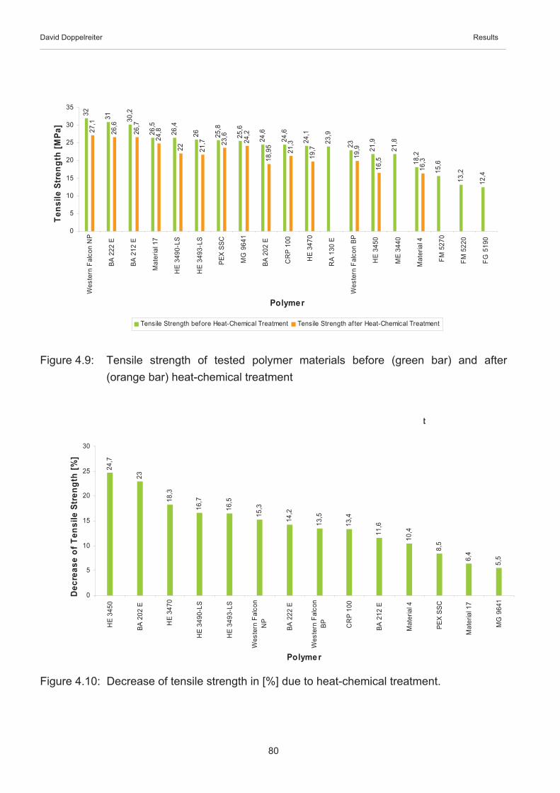
David Doppelreiter Results
80
Figure 4.9: Tensile strength of tested polymer materials before (green bar) and after (orange bar) heat-chemical treatment
Figure 4.10: Decrease of tensile strength in [%] due to heat-chemical treatment.
Decrease of Tensile Strength due to Heat-Chemical Treatment
24,7
23
18,3
16,7
16,5
15,3
14,2
13,5
13,4
11,6
10,4
8,5
6,4
5,5
0
5
10
15
20
25
30
HE
3450
BA 2
02 E
HE
3470
HE
3490
-LS
HE
3493
-LS
Wes
tern
Fal
con
NP
BA 2
22 E
Wes
tern
Fal
con
BP CR
P 10
0
BA 2
12 E
Mat
eria
l 4
PEX
SSC
Mat
eria
l 17
MG
964
1
Polymer
Dec
reas
e of
Ten
sile
Str
engt
h [%
]Tensile Strength be fore and afte r Heat-chemical Treatment
32 31 30,2
26,5
26,4
26 25,8
25,6
24,6
24,6
24,1
23,9
23 21,9
21,8
18,2
15,6
13,2
12,4
27,1
26,6
26,7
24,8
22 21,7 23
,6
24,2
18,9
5
21,3
19,7
19,9
16,5
16,3
0
5
10
15
20
25
30
35
Wes
tern
Fal
con
NP
BA 2
22 E
BA 2
12 E
Mat
eria
l 17
HE
3490
-LS
HE
3493
-LS
PEX
SSC
MG
964
1
BA 2
02 E
CR
P 10
0
HE
3470
RA
130
E
Wes
tern
Fal
con
BP
HE
3450
ME
3440
Mat
eria
l 4
FM 5
270
FM 5
220
FG 5
190
Polymer
Tens
ile S
tren
gth
[MPa
]
Tensile Strength before Heat-Chemical Treatment Tensile Strength af ter Heat-Chemical Treatment

David Doppelreiter Results
81
28,4
5
26,9
1
23,9
23,6
6
23,3
22,6
5
22,3
2
21,1
2
20,7
4
20,2
3
19,4
3
18,8
9
17,7
17,5
3
16,9
9
13,8
6
11,7
10,1
6
8,85
13,4
11,7 13
,4 14,1
14,5 16
,9
6,8
18,9
14,2
10,9 12
,3
10,8
10,4
10,8
0
5
10
15
20
25
30BA
212
E
BA 2
22 E
Wes
tern
Fal
con
NP
HE
3493
-LS
HE
3490
-LS
MG
964
1
BA 2
02 E
Mat
eria
l 17
PEX
SSC
HE
3470
CR
P 10
0
Wes
tern
Fal
con
BP
RA
130
E
ME
3440
HE
3450
Mat
eria
l 4
FM 5
270
FM 5
220
FG 5
190
Polymer
Yiel
d st
reng
th [M
Pa]
Yield strength before Heat-Chemical Treatment Yield strength after Heat-Chemical Treatment
Figure 4.11: Yield strength of tested polymer materials before (green bar) and after (orange bar) heat-chemical treatment
Figure 4.12: Decrease of yield strength in [%] due to heat-chemical treatment
69,5
56,5
52,9
46,1
43,9
42,8
40,4
38,8
37,8
36,7
31,5
25,4
22,1
10,5
0
10
20
30
40
50
60
70
80
BA 2
02 E
BA 2
22 E
BA 2
12 E
HE
3470
Wes
tern
Fal
con
NP
Wes
tern
Fal
con
BP
HE
3493
-LS
HE
3450
HE
3490
-LS
CR
P 10
0
PEX
SSC
MG
964
1
Mat
eria
l 4
Mat
eria
l 17
Polymer
Dec
reas
e of
yie
ld s
tren
gth
[%]

David Doppelreiter Results
82
4.4 Values given by Borealis
Figure 4.13 points the density of the different types of polymers. The highest densities are reached by high density polyethylene compared to the low values by polypropylene. This is caused by the different chemical composition of this two dissimilar types of polymers (see chapter 3.1.1).
In Figure 4.14 the weight average-molecular weight (Mw) data (see chapter 2.4.3.2) of some polymer materials (polyethylene) is shown. Unfortunately not all values of the weight average-molecular weight for the other types of polymer materials were available (by Borealis) and therefore it was not possible to complete this chart. High density polyethylene possesses the highest values for weight average-molecular weight, which is the biggest difference between high and low density polyethylene.
The number average-molecular weight (Mn) is shown in Figure 4.15 and just a few values were available like in Figure 4.14 (but for the same types of polymers). Now the low density polyethylene presents higher values and this indicates a narrow distribution of molecular weights.
Figure 4.16 shows some values for abrasion determined by a Taber test. The placing of many polymer materials does not correlate with the results made by abrasion testing in OMV laboratories.

David Doppelreiter Results
83
Figure 4.13: Density of different polymer materials except Western Falcon Natural pipe.
Figure 4.14: Weight average – molecular weight [g/mol] for some polymer materials (polyethylene). All data provided by Borealis.
Weight Average-Molecular Weight
3700
00
3300
00
3290
00
3290
00
3290
00
2540
00
1620
00
1440
00
1400
00
1330
00
0
50000
100000
150000
200000
250000
300000
350000
400000
Mat
eria
l 17
HE
3493
-LS
HE
3490
-LS
HE
3470
ME
3440
PEX
SSC
FM 5
220
FM 5
270
Mat
eria
l 4
FG 5
190
Polymer
wei
ght a
vera
ge -
Mol
ecul
ar W
eigh
t [g
/mol
]Density of different Polymer Materials
964
959
955
952
951
950
950
946
946
942
934
927
922
919
915
905
900
900
860
880
900
920
940
960
980
MG
964
1
CR
P 10
0
Wes
tern
Fal
con
BP
Mat
eria
l 17
ME
3440
HE
3490
-LS
HE
3493
-LS
PEX
SSC
HE
3470
HE
3450
Mat
eria
l 4
FM 5
270
FM 5
220
FG 5
190
BA 2
22 E
RA
130
E
BA 2
12 E
BA 2
02 E
Polymer
Den
sity
[kg/
m³]

David Doppelreiter Results
84
Figure 4.15: Number average – molecular weight [g/mol] for some polymer materials (polyethylene). All data provided by Borealis.
Figure 4.16: Taber abrasion values for some polymer materials
Number Average - M olecular Weight
8700
0
5586
2
4645
2
4600
0
2955
6
1000
0
7000
6714
6714
6714
0
10000
20000
30000
40000
50000
60000
70000
80000
90000
100000PE
X SS
C
FM 5
220
FM 5
270
Mat
eria
l 4
FG 5
190
Mat
eria
l 17
HE
3493
-LS
HE
3490
-LS
HE
3470
ME
3440
Polymer
num
ber a
vera
ge -
Mol
ecul
ar W
eigh
t [g
/mol
]
3,3
8,3 9,3 10
,5 12
14,1
14,4 15
,9
16 16,8
1
18,2
39,7
0
5
10
15
20
25
30
35
40
45
PEX
SSC
HE
3490
-LS
Mat
eria
l 4
HE
3450
Wes
tern
Falc
on B
P
HE
3493
-LS
MG
964
1
FG 5
190
BA 2
12 E
FM 5
220
Wes
tern
Falc
on N
P
Mat
eria
l 17
Polymer
Tabe
r Abr
asio
n

David Doppelreiter Results
85
4.5 Calculated values
The crystallinity as well as the polydispersity index (PDI) was calculated by following equations:
Crystallinity [25]:
���
����
�����
����
�
���
����
�����
����
�
�
ac
aCP
''
''11
11
(Equ. 4.1)
Table 4.1 Density of amorphous ('a) and crystalline ('c) phase of polyethylene and polypropylene
PolymerDensity 'a [kg/m³]
Density 'c
[kg/m³] Polyethylene 853 1004
Polypropylene 850 950
Polydispersity Index (PDI):
n
w
MM
PDI � (Equ. 4.2)
Figure 4.17 presents the crystallinity of all tested polymer materials except Western Falcon Natural Pipe. For this type of polymer no density value was available therefore a determination of the crystallinity was not possible.
Figure 4.18 demonstrates the calculated values of the Polydispersity Index (PDI). This index illustrates the broadness of the molecular weight distribution of a polymer material. As already mentioned in Figure 4.15 the high values for the number average-molecular weight for LLDPE in comparison to the weight average-molecular weight results in low values for the PDI. This means simultaneously a narrow distribution of the molecular weight. The opposite result is shown for HDPE and therefore a broad distribution is obtained. This conclusion should result in less wear for LLDPE due to the narrow distribution but Figure 4.1 indicates the opposite. This could be explained by the low weight average-molecular weight of LLDPE
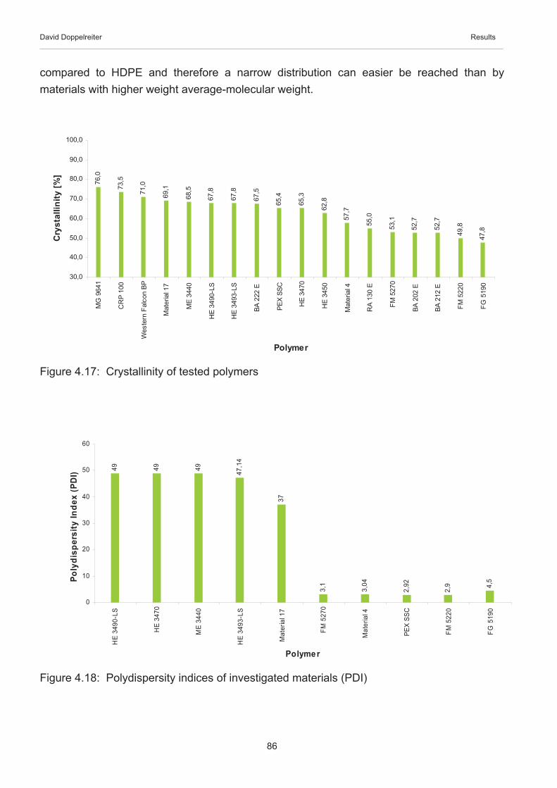
David Doppelreiter Results
86
compared to HDPE and therefore a narrow distribution can easier be reached than by materials with higher weight average-molecular weight.
Figure 4.17: Crystallinity of tested polymers
Figure 4.18: Polydispersity indices of investigated materials (PDI)
Polydispersity
49 49 49 47,1
4
37
3,1
3,04
2,92
2,9 4,
5
0
10
20
30
40
50
60
HE
3490
-LS
HE
3470
ME
3440
HE
3493
-LS
Mat
eria
l 17
FM 5
270
Mat
eria
l 4
PEX
SSC
FM 5
220
FG 5
190
Polymer
Poly
disp
ersi
ty In
dex
(PD
I)
Crystallinity
76,0
73,5
71,0
69,1
68,5
67,8
67,8
67,5
65,4
65,3
62,8
57,7
55,0
53,1
52,7
52,7
49,8
47,8
30,0
40,0
50,0
60,0
70,0
80,0
90,0
100,0
MG
964
1
CR
P 10
0
Wes
tern
Fal
con
BP
Mat
eria
l 17
ME
3440
HE
3490
-LS
HE
3493
-LS
BA 2
22 E
PEX
SSC
HE
3470
HE
3450
Mat
eria
l 4
RA
130
E
FM 5
270
BA 2
02 E
BA 2
12 E
FM 5
220
FG 5
190
Polymer
Cry
stal
linity
[%]

David Doppelreiter Results
87
4.6 Interrelationship of results and different polymer properties
The following charts indicate some results due to the physical properties of the different polymer materials.
Figure 4.19 illustrates the coherence between the AWR of all polymer materials (polyethylene and polypropylene) and the yield strength. The AWR was determined by the use of spray metal couplings as counterpart, a rotation of 345 rpm, a load of 130 kg and a temperature of 50°C. A clearly dependence is shown by this chart – high values for yield strength results in low AWR. This big dependence of the AWR can be explained by the low factor of abrasion due to the smooth surface of the spray metal coupling. Because of the high load of 130 kg during the testing procedure the polymer materials started to creep at the in- and outside of the wear track. This shoulders were bigger for soft materials as for harder. So for the use of spray metal couplings abrasion is very low and therefore the material with the lowest tendency to creep will be the best. More information about the wear mechanism will be found in chapter 5.
Figure 4.20 represents the AWR against the tensile strength. Polymer materials with higher tensile strength showed the best wear behaviour.
As expected due to the relation between hardness and tensile strength or yield strength Figure 4.21 is displaying the similar behaviour of polymers like in Figure 4.19 or Figure 4.20. Polymers with higher hardness showed less creep and therefore less AWR.
Figure 4.22 is again presenting the relation between AWR and shore D hardness. Unlike Figure 4.21 the values for the AWR were determined by the use of sand particles in the medium. Therefore materials with lower hardness showed better wear behaviour than harder one. This can be explained through the higher chance for sand grains to embed in the surface of the material.
Figure 4.23 shows the relationship between the yield strength and the weight average-molecular weight of polyethylene materials (only these data were available by Borealis). Higher weight average-molecular weight indicates longer chains resulting in more physical cross-links and better mechanical and long-time properties. Due to the dependency of long-time behaviour on the weight average–molecular weight more information on polypropylene materials are required. This chart shows, as described in literature, a higher value for yield strength by increasing weight average-molecular weight data.

David Doppelreiter Results
88
For tensile strength versus weight average-molecular weight Figure 4.24 illustrates a similar profile like Figure 4.23.
In Figure 4.25 density is plotted versus yield strength for polyethylene and polypropylene. For both species the values for yield strength are higher with increasing density. Because of differences in chemical structure polypropylene always has lower values of density than polyethylene.
Density versus tensile strength for polyethylene and polypropylene materials is plotted in Figure 4.26. An equal tendency like in Figure 4.25 can be found namely increasing tensile strength with higher density values.
Figure 4.27 demonstrates the dependency of the density and the decrease of the yield strength due to heat-chemical treatment for tested polymer materials. This decrease is indirect proportional to the density and materials with low density values like polypropylene showed the highest decrease followed by linear low density polymers. This high decrease is an important topic in case of creep. As mentioned above polypropylene materials reached the lowest AWR by the use of spray metal couplings due to less creep but this can be changed if this materials loose their stiffness during operation in field as simulated during testing procedure.
Similar behaviour can be found in Figure 4.28 where density is plotted against the decrease of tensile strength due to heat-chemical treatment. Polymers with higher density values show more resistance to decrease than polymers with low density values.
Figure 4.29 ratifies the assumption that materials with low density are more susceptible for swelling due to heat-chemical treatment. The swelling was determined by the difference of the weight before and after treatment. This result correlates well with Figure 4.27 and Figure 4.28 and indicates, that swelling is depending on density and strongly affects the mechanical properties of low density materials.

David Doppelreiter Results
89
0,00
0,20
0,40
0,60
0,80
1,00
1,20
1,40
1,60
1,80
0 5 10 15 20 25 30
Yield strength [MPa]
Are
a w
ear r
ate
[mm
²/a]
Figure 4.19: AWR, due to sliding contact of different polymer materials on spray metal couplings (Ra~0.1µm) at 345 rpm, 50°C, and a load of 130 kg, is plotted against the Yield strength.
0,00
0,20
0,40
0,60
0,80
1,00
1,20
1,40
1,60
1,80
0 5 10 15 20 25 30 35
Tensile Strength [MPa]
Are
a w
ear r
ate
[mm
²/a]
Figure 4.20: AWR, due to sliding contact of different polymer materials on spray metal couplings (Ra~0.1µm) at 345 rpm, 50°C, and a load of 130 kg, is plotted against the Tensile strength.

David Doppelreiter Results
90
0,00
0,20
0,40
0,60
0,80
1,00
1,20
1,40
1,60
1,80
50 55 60 65 70 75
Shore D Hardness
Are
a w
ear r
ate
[mm
²/a]
Figure 4.21: AWR, due to sliding contact of different polymer materials on spray metal couplings (Ra~0.1µm) at 345 rpm, 50°C, and a load of 130 kg, is plotted against the Shore D Hardness.
0
2
4
6
8
10
12
14
62 63 64 65 66 67 68 69 70 71 72 73
Shore D Hardness
Are
a w
ear r
ate
[mm
²/a]
Figure 4.22: AWR, due to sliding contact of different polymer materials on spray metal couplings (Ra~0.1µm) including sand particles at 345 rpm, 50°C, and a load of 130 kg, is plotted against the Shore D Hardness.

David Doppelreiter Results
91
0
5
10
15
20
25
30
0 50000 100000 150000 200000 250000 300000 350000 400000
weight average-molecular weight [g/mol]
Yiel
d st
reng
th [M
Pa]
polyethylene
Figure 4.23: Yield strength against weight average-molecular weight of polyethylene materials.
0
5
10
15
20
25
30
0 50000 100000 150000 200000 250000 300000 350000 400000
weight average-molecular weight [g/mol]
Tens
ile S
tren
gth
[MPa
]
polyethylene
Figure 4.24: Tensile strength against weight average-molecular weight of polyethylene materials.

David Doppelreiter Results
92
890
900
910
920
930
940
950
960
970
0 5 10 15 20 25 30 35 40
Yield strength [MPa]
Den
isty
[kg/
m³]
polyethylene polypropylene
Figure 4.25: Density versus yield strength for polyethylene (green) as well as for polypropylene (orange) materials.
880
890
900
910
920
930
940
950
960
970
0 5 10 15 20 25 30 35 40
Tensile Strength [MPa]
Den
sity
[kg/
m³]
polyethylene polypropylene
Figure 4.26: Density versus tensile strength for polyethylene (green) as well as for polypropylene (orange) materials.
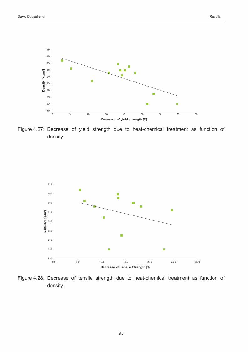
David Doppelreiter Results
93
890
900
910
920
930
940
950
960
970
980
0 10 20 30 40 50 60 70 80
Decrease of yield strength [%]
Den
sity
[kg/
m³]
Figure 4.27: Decrease of yield strength due to heat-chemical treatment as function of density.
890
900
910
920
930
940
950
960
970
0,0 5,0 10,0 15,0 20,0 25,0 30,0
Decrease of Tensile Strength [%]
Den
sity
[kg/
m³]
Figure 4.28: Decrease of tensile strength due to heat-chemical treatment as function of density.

David Doppelreiter Results
94
890
900
910
920
930
940
950
960
970
0 2 4 6 8 10 12 14
Increase of weight [%]
Den
sity
[kg/
m³]
Figure 4.29: Increase of weight due to heat-chemical treatment against density.

David Doppelreiter Results
95
4.7 Scanning Electron Microscopy
The following surface images were taken by the SEM in the OMV laboratories (3.5.4). Pictures of the wear track generated by sliding contact to spray metal couplings, with or without sand, or polyamide rod centralizer, with or without sand, were made of each tested polymer. Images of polymer surfaces damaged by the use of unalloyed steel couplings were gained thus a previous work [19]. Further images were made of used sand (Quarzwerke Österreich) and original produced sand out of a formation.
The different polymer species showed basically 4 different types of wear tracks depending on the counterpart (spray metal coupling or rod centralizer) and the appearance of sand particles. This prediction is supported by a significant change in wear rates by the use of different counterparts. Therefore these 4 different types are shown in the following pictures.
Figure 4.30 shows the wear track of the high density polyethylene HE 3490-LS by the use of spray metal couplings without sand particles. No appreciable abrasion mechanism occurs but the presence of many small holes indicate surface fatigue as wear mechanism. The diameter of these holes is approximately 10 µm. For linear low density polyethylene materials the number of holes is smaller by the same diameter.
In Figure 4.31 spray metal couplings were used including sand particles. As expected the damage of surface increased as mentioned in Figure 4.3 by the change of wear mechanism from fatigue to abrasion. Beside the wear track generated by abrasion in the center of picture 1, beam wear occurs. This wear mechanism is caused by a sand beam which is injected by small metal pipes (see Figure 3.3) directly under the polymer plate in the pilot plant. Picture 2 and 3 show the embedded sand grains the polymer matrix. This happens due to the high hardness difference between spray metal couplings and the liner material. Because of this mechanism the damage of the polymer material can be reduced.
Figure 4.32 is a SEM image of the wear track by the use of polyamide rod centralizer without sand. For this combination of materials abrasion is the main wear mechanism. This can be explained by the weakness of the intermolecular bonds of polymer materials compared to metals. The origin for this kind of wear mechanism is the weakness of the intermolecular bonds of polymer materials compared to metals. The reason for less wear by sliding against spray metal couplings is the high hardness of the spray metal layer due to no wear debris occur. In case of sliding against polyamide rod centralizer this high hardness can not be obtained by this kind of material and thus friction forces generate wear debris. These great amounts of wear particles which are formed during the whole testing period are responsible

David Doppelreiter Results
96
for the dramatic high rate of abrasion and can only be dropped by a completely new type of rod centralizer.
Figure 4.33 demonstrates the wear track by the use of polyamide rod centralizer including sand particles. The wear mechanism is similar to Figure 4.32 namely abrasion. Unlike in Figure 4.31 the sand grains are not embedded. This can be explained by the lower hardness difference between the centralizer and the liner material and therefore higher wear rates are obtained.
Figure 4.34 and Figure 4.35 represent two different types of sand. Figure 4.34 shows the tested kind of sand (“Quarzwerke Österreich”) which was used for testing. Figure 4.35 displays an originally produced sand from the Vienna basin. The produced sand shows wider distribution of the grain size and lower angularity than the used one. This wider distribution indicates maybe more problems for the liner material due to the dependence of the abrasivity of a particle from its size. Bigger grains will cause more damage than smaller ones (2.4.3.7). Also important for the abrasivity of a particle is its angularity or sharpness and as indicated in Figure 4.36 the shape of the produced sand grains is spheroidal. This spheroidal shape indicates less abrasivity and therefore less damage to the polymer. So it is not possible to predict which type of sand will be more or less abrasive for the liner material due to the different size distribution and angularity.

David Doppelreiter Results
97
Figure 4.30: Wear track generated by the use of spray metal couplings without sand particles (HE 3490-LS).

David Doppelreiter Results
98
Figure 4.31: Wear track generated by the use of spray metal couplings with sand particles. As we can see in picture 2 and 3 some sand particles are embedded in the polymer matrix (HE 3490-LS).

David Doppelreiter Results
99
Figure 4.32: Wear track generated by the use of polyamide rod centralizer (HE 3490-LS).

David Doppelreiter Results
100
Figure 4.33: Wear track generated by the use of polyamide rod centralizer with sand particles (HE 3490-LS).

David Doppelreiter Results
101
Figure 4.34: SEM picture of used sand for testing (Quarzwerke Österreich)
Figure 4.35: Original produced sand of the vienna basin. The original sand shows much lower angularity and a wider size distribution than the used one.

David Doppelreiter Results
102
Figure 4.36: A higher magnification of the originally produced sand indicates clearly the low angularity of this type of sand.

David Doppelreiter Discussion
103
5 Discussion
The emphasis of this work was the determination of the wear behaviour for different polymer species in sliding contact to spray metal couplings. Furthermore some tests including sand particles in the medium were conducted and the behaviour in sliding contact to polyamide rod centralizers was analyzed. Due to all these tests big differences in the wear behaviour occurred as shown in Figure 4.6. Sliding contact with spray metal couplings without sand particles showed the lowest AWR followed by unalloyed steel couplings (without sand) and spray metal couplings with sand particles. The taillight was represented by the sliding contact with polyamide rod centralizers. The next lines should be used for the discussion of these different results.
5.1 Sliding contact of polymer samples versus spray metal couplings
The low values of wear rate in Figure 4.2 are based on the smooth and very hard surface of the coupling. As mentioned in chapter 2.4.3 polymers have some friction properties that can not be obtained by any group of materials. These good friction properties are based on the low surface energy due to the weak intermolecular bonds separation is easy even by moderate friction. Therefore polymers are very susceptible in case of wear. Especially in case of high roughness of harder materials against polymers they get destroyed quite fast by abrasion. In Figure 2.30 very low roughness, as it is the case for spray metal couplings, should result again in higher friction coefficient due to increasing contact area and therefore higher values for adhesion. But because of the low surface energies of the polymers and the presence of an oxide layer on the spray metal surface and an oil, water mixture, as lubricant, adhesion is negligible. This fact results in weak friction forces demanding the polymer surface and therefore less wear. In case of this combination the marginal roughness of the coupling (Ra~0.1) causes slight deformation on the polymer surface which can cause surface fatigue. This wear mechanism is approved by different SEM images of the wear tracks (see Figure 4.30). As well as low adhesion the high surface hardness of the spray metal layer is very important for less wear. By reason of this high hardness no wear debris is generated and therefore no abrasion will occur. Due to these mechanisms wear is more or less eliminated and the differences in AWR of polymer species are smaller compared to unalloyed steel couplings ([19] or Figure 4.1). The performance of all tested polymer species was highly influenced by the tendency to creep because of the high load (130 kg) during testing and the low wear rates. By reason of
David Doppelreiter Discussion
104
very low wear rates the appearance of creep shoulders on the in- and outside of the wear track influenced the evaluation much stronger than in tests with high abrasion rates (e.g.: sliding contact against polyamide rod centralizer). Therefore materials with high stiffness reached the best values by the use of spray metal couplings but these results are relativised by the heat-chemical treatment tests (4.3). In these tests most of the materials with high stiffness, especially polypropylene, lost their high values for yield strength or tensile strength due to swelling and thus a large observation of all test results is required before any decision about the choice of a liner material can be made.Summarized it can be said that an application of spray metal couplings is necessary by the use of relined production tubings to minimize the mechnical wear damage during operation and to reach a maximum lifetime.
5.2 Sliding contact of polymer samples versus spray metal couplings including sand particles in the medium
As for every tribology system sand grains are responsible for higher damage of contact area and thus decreasing lifetime. By use of spray metal couplings as sliding contact to a polymer sample in a fluid including sand particles the wear mechanism changes from fatigue to abrasion, resulting in an increase of wear rates and a contraction of lifetime. But as claimed in literature polymer and rubber materials show more abrasion-resistance against solid particles than metals due to embedding of solid particles. By the inspection of the SEM pictures this embedding of sand grains can be observed as well as the abrasion mechanisms, like micro-ploughing or micro chipping (2.4.3.6), if no embedding can be reached. Due to high differences in hardness between spray metal coupling and polymer material a high grade of embedding can be reached and therefore a low damage of polymer surface can be obtained (see Figure 4.31).Polymer materials with lower hardness showed lower abrasion values (Figure 4.22) than harder ones but more tests need to be done to assure these results. Because of the high impact of size, hardness and sharpness or angularity of the particles on abrasion (2.4.3.7) further tests including original formation sand would be necessary.
5.3 Sliding contact of polymer samples versus polyamide rod centralizer
After promising results for spray metal couplings the wear behaviour of polymer materials in sliding contact to polyamide rod centralizers was wasteful. The AWR were 1000 times higher than for spray metal couplings.The origin of these big wear rates is the weakness of the intermolecular bonds of polymer materials compared to metals. As mentioned above the reason for less wear by sliding

David Doppelreiter Discussion
105
against spray metal couplings is the hardness of the spray metal layer. In case of sliding against polyamide rod centralizer this high hardness can not be obtained by this kind of material and thus friction forces generate a lot of wear debris. These great amounts of wear particles which are formed during the whole testing period are responsible for the dramatic high rate of abrasion and can only be dropped by a completely new type of rod centralizer (see Figure 4.32).
5.4 Sliding contact of polymer samples versus polyamide rod centralizer including sand particles in the medium
Due to the addition of sand particles the values for the AWR (Figure 4.22) are higher. Not only the creation of wear particles during sliding contact between the polyamide rod centralizer and the polyolefin tubing material but also the sand particles are responsible for the high damage of the materials and therefore an adoption into field is not imaginable.
Finally it can be said that the application of relined tubings is very promising by the use of spray metal couplings and an abdication of rod centralizers. If rod centralizers are required much more investigation is necessary to reduce the abrasion for the tubing material.
David Doppelreiter Conclusion
106
6 Conclusion
Relined tubings indicate a very promising new technology for increasing lifetime of sucker rod pumps and therefore reduced workover and production costs. By the use of relined production tubings a lot of requirements must be achieved by the liner material like high resistance against abrasion, high resistance against elevated temperatures, good long-time properties, a low price of the raw material, and an easy producibility. Many abrasion and heat-chemical treatment tests (see chapter 4) were realized in the OMV laboratories to characterize the different materials concerning these requirements. The most important topic was the wear behaviour of the different polymer materials against 3 different types of sliding contact partners like unalloyed steel couplings, spray metal couplings and polyamide rod centralizers followed by the evaluation of long-time properties of these materials.16 different polyolefin materials were tested concerning their wear behaviour in sliding contact to unalloyed steel couplings (Ra~3µm) by a previous [19] and 3 during this work.The best materials were distinguished by their high density (for polyethylene), high crystallinity and high molecular weight. The main goal of this work was the characterisation of the wear behaviour under sliding contact to spray metal couplings (Ra~0.1µm) which is shown in Figure 4.2.16 different materials were tested with the best results for PEX SSC (polyethylene) and BA 202 E (polypropylene) materials. By the use of spray metal couplings the wear rate dropped down by the factor ~10 to ~50 despite the double load of 130 kg. This can be explained by the low roughness of the spray metal coupling and the low adhesion forces between the coupling and the polymer due to the low surface energy of the polymer material, an oxidlayer on the spray metal surface and the presence of an oil-water mixture as lubricant as well as the high hardness of the spray metal layer and thus no wear particle appearance. In case of this combination just the marginal roughness of the coupling (Ra~0.1) introduces lowly deformation into the polymer surface which can cause surface fatigue and this wear mechanism is approved by different SEM images of the wear tracks. These data provide successful oil production with increasing lifetime of tubings. The introduction of sand grains results in higher wear rates by a change of the wear mechanism from fatigue to abrasion. Out of these tests it is not really possible to quantify the impact on lifetime so maybe longer testing periods in the pilot plant or tests in field would lead to more significant results. The used sand particles from “Quarzwerke Österreich” have more or less the same size distribution but other values for the sharpness or angularity (SEM images) than sand grains out of real formations. For further tests the used sand should be displaced by real sand particles out of formations.
David Doppelreiter Conclusion
107
The application of polyamide rod centralizer should be neglected because of dramatic high damages on the liner material (Figure 4.4). The big difference of spray metal couplings to polyamide rod centralizer concerning wear behaviour against the liner material is the different type of material. Polyamide is a polymer and therefore lower intermolecular forces can be achieved compared to metallic materials. Due to this difference even small friction forces between the liner (polyethylene or polypropylene) and the rod centralizer (polyamide) material can lead to a high amount of wear particles. These wear particles are the reason for the extremely high abrasion rates. The addition of sand particles intensifies the wear by the factor ~2. Since the liner materials are not only demanded by friction and wear, the presence of elevated temperatures, hydrocarbons and water also limits the long-time properties. Some tests in autoclaves (3.5.6) were made for one week by the use of an oil-water mixture, 10 bar CO2 and elevated temperatures of 70°C. The results are summarized in Figure 4.25 to Figure 4.29.
On closer examination of some important test results there is no polymer which scored similar well or bad in all of these different tests like it is indicated in Figure 6.1. Therefore an average of all test results (4 different kinds of tests – see Figure 6.1) of all different polymers (just this species where these 4 different tests were made) was calculated and is shown in Figure 6.2. PEX SSC, a high density polyethylene and cross-linked prototype, reached after addition of all different results the first place followed by 4 species of high density polyethylene materials.
Finally it can be said, that if the technology of relined tubings will get any possibility for application in oil production the use of high density cross-linked polyethylene as liner material is essential for a successful operation.

David Doppelreiter Conclusion
108
12
34
56
78
910
1112
1314
1
9
5
14
12
4
23
8
67
13
1011
3
5
11
78
13
109
21
12
4
6
14
4
11
5
8
1314
7
9
1
3
10
2
4
6
0
2
4
6
8
10
12
14
16
PEX
SSC
BA 2
12 E
HE
3490
-LS
Wes
tern
Falc
on B
P
BA 2
22 E
BA 2
02 E
HE
3493
-LS
Wes
tern
Falc
on N
P
Mat
eria
l 17
MG
964
1
HE
3470
Mat
eria
l 4
CR
P 10
0
HE
3450
Polymer
Ran
king
[num
ber]
Ranking - Polymer vs. spray metal couplingRanking - Polymer vs. unalloyed steel coupling
Ranking - Decrease of tensile strength due to heat-chemical treatmentRanking - Decrease of yield strength due to heat-chemical treatment
Figure 6.1: Ranking of different types of polymers for different types of testing procedures.
1
2 2
3
4
5
6
7
8 8
9
10
11
12
0
2
4
6
8
10
12
14
PEX
SSC
Mat
eria
l 17
MG
964
1
HE
3490
-LS
HE
3493
-LS
BA 2
12 E
Wes
tern
Fal
con
NP
Mat
eria
l 4
CR
P 10
0
Wes
tern
Fal
con
BP BA 2
02 E
BA 2
22 E
HE
3470
HE
3450
Polymer
Ran
king
[num
ber]
Figure 6.2: Summarized ranking due to addition of each ranking

David Doppelreiter Outlook
109
7 Outlook
A lot of polymers were characterized in the past months on their resistance to abrasion and elevated temperatures under simultaneous chemical treatment. After summarizing all results high density cross-linked polyethylene showed the best performance and therefore more different species of these materials should be tested in the future.Furthermore tests including sand particles are necessary but by the addition of original sand out of formations unlike the synthetic sand used during this work. The use of a polyamide rod centralizer in relined tubings has to be neglected due to the high damage for the liner material as shown in Figure 4.4. If rod centralizers are still required in sucker rod units a lot of investigation has to be done to create a new type of centralizer to reduce the abrasion rates for the polyolefin liner material.

Dav
id D
oppe
lreite
r
A
ppen
dix
110
8 A
ppen
dix
8.1
App
endi
x A
Figu
re 8
.1:
Che
mic
al a
naly
se b
y O
MV
labo
rato
ry o
f use
d sa
nd (c
ompa
ny Q
uarz
wer
ke Ö
ster
reic
h)
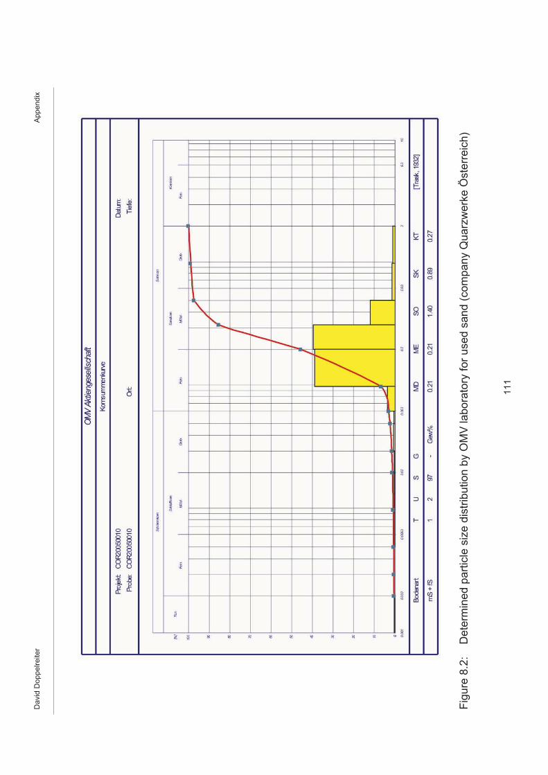
Dav
id D
oppe
lreite
r
A
ppen
dix
111
Figu
re 8
.2:
Det
erm
ined
par
ticle
siz
e di
strib
utio
n by
OM
V la
bora
tory
for u
sed
sand
(com
pany
Qua
rzw
erke
Öst
erre
ich)

David Doppelreiter Literature
112
9 Literature
[1] SBS Ölfördergeräte: “Erdölförderung mit Gestängetiefpumpen”, Vereinigte Edelstahlwerke AG, Ternitz, 1984, p. 10-58, 100
[2] G. Mori: “Skriptum zur Vorlesung Korrosionskunde”, Institut für Allgemeine und Analytische Chemie, Leoben, 2003, p. 4
[3] NACE TPC Publication No. 5: “Corrosion Control in Petroleum Production”, National Association of Corrosion Engineers, Houston, 1979, p. 47 – 53
[4] Advantica Ltd.: “Performance Review: The best lining system in the world”, Ashby Road, Loughborough, Leictershire LE 11 3GL, England, http://www.advantica.biz, December 2006
[5] G. W. Stachowiak, A. W. Bachelor: “Engineering Tribology”, Butterworth-Heinemann, 2001, p. 1-8, 447-478, 483-527, 533-568, 571-590, 619-663
[6] B. Bushan: in “Handbook of Micro / Nano Tribology”, (ed. B. Bushan), CRC Press LLC, 1999, p. 3-81.
[7] Ernest Rabinowicz: “Friction and Wear of Materials”, John Wiley & Sons, Inc, 1995, p. 1-14, 44-65
[8] H. Uetz, J. Wiedemayer: “Tribologie der Polymere”, Carl Hanser Verlag, München – Wien, 1985, p. 95
[9] G. Fleischer: “Grundlagen zu Reibung und Verschleiß”, VEB Deutscher Verlag für Grundstoffindustrie, Leipzig, 1978, p. 141
[10] H. Czichos, K. H. Habig: ”Tribologie – Handbuch“, Vieweg & Sohn Verlag, Wiesbaden, 2003, p. 19-74, 81-108, 113-160
[11] Hans-Georg Elias: „An Introduction to Polymer Science“, VCH Verlagsgesellschaft mbH, Weinheim, 1997, p. 23-32, 344-354

David Doppelreiter Literature
113
[12] E. Hornbogen, K. Schäfer: in „Fundamentals of friction and wear of materials“, (ed. D. A. Rigney), American Society for Metals, 1981, p. 409-438
[13] University of Southern Mississippi, http://www.pslc.ws/mactest/weight.htm,January 2007
[14] Wikipedia Foundation, Inc., http://en.wikipedia.org/wiki/Polyethylene, January 2007
[15] P. Eyerer, P. Elsner, Th. Hirth: “Die Kunststoffe und ihre Eigenschaften”, Springer-Verlag Berlin Heidelberg, 2005, p. 455-603
[16] G.W. Stachowiak, D.V. de Pellegrin, P. Podsiadlo: „Wear-Materials, Mechanims and Practice“, (ed. G.W. Stachowiak), John Wiley & Sons Ltd, Chichester, 2005, p. 339-365
[17] Larssen – Basse: “Some Effects of Specimen Size of Abrasive Wear”, Wear, 19, 1972, 27-35
[18] Borealis, http://www.boralisgroup.com, February 2007
[19] R. Sonnleitner: “Enhanced Performance of Sucker Rod Pumps”, Leoben, May 2006
[20] API Specification 11B: “Specification of Sucker Rods”, American Petroleum Institute, twenty-sixth edition, January 1998
[21] http://www.corrosion.com/thermal-sec1.html, January 2007
[22] MatWeb, http://www.matweb.com/reference/shore-hardness.asp, January 2007
[23] Fries Research & Technology GmbH, http://www.frt-gmbh.com/frt/upload/pdf_en /FRT_Brochure_EN.pdf, January 2007
[24] Annual Book of ASTM Standards Volume 08.01: “Standard Test Method for Tensile Properties of Plastics”, ASTM D638-00, ASTM, West Conshocken, 2001

David Doppelreiter Literature
114
[25] National Science Foundation, Camille and Henry Dreyfus Foundation, PCOL faculty, http : // faculty . uscupstate . edu / llever / Polymer % 20Resources /Density.htm # percent, January 2007
[26] Wikipedia Foundation, Inc., http://en.wikipedia.org/wiki/Scanning_electron_ microscope, January 2007