increasing returns and all that (antweiler and trefler, 2002)
TRANSCRIPT

8/3/2019 Increasing Returns and All That (Antweiler and Trefler, 2002)
http://slidepdf.com/reader/full/increasing-returns-and-all-that-antweiler-and-trefler-2002 1/59
1%(5:25.,1*3$3(56(5,(6
,1&5($6,1*5(78516$1'$//7+$7
$9,(:)52075$'(
:HUQHU$QWZHLOHU
'DQLHO7UHIOHU
:RUNLQJ3DSHU
KWWSZZZQEHURUJSDSHUVZ
1$7,21$/%85($82)(&2120,&5(6($5&+
0DVVDKXVHWWV$YHQXH
&DPEULGJH0$
2WREHU
:HKDYHEHQHILWHGIURPWKH.RPPHQWVRIHQ$UURZ'RQ'DYLV0HO)XVV*HQH*URVVPDQ(OKDQDQ
+HOSPDQ'DOH-RUJHQVRQ3DXOUXJPDQ5L.KDUG/LSVH\$QJHOR0HOLQR$ULHO3DNHV1DWKDQ5RVHQEHUJ
6.RWW7D\ORUDQG'DYLG:HLQVWHLQDVZHOODVVHPLQDUSDUWL.LSDQWVDW&,$5+DUYDUG0,77RURQWR8%&
DQG<DOH$ORQJWKH\HDUSDWKRIGDWD.ROOH.WLRQZHKDYH.KDONHGXSGHEWVWR&KULV7KRUQEHUJIRUROGHU
&36GDWDWR5REHUW%DUURDQG-RQJ:KD/HHIRUHGX.DWLRQGDWDWR5RJHU7KHLUULHQRI6WDWLVWL.V&DQDGDIRU
WUDGHGDWDWR5REHUW6XPPHUVDQG$ODQ+HVWRQIRUWKH3HQQ:RUOG7DEOHVDQGWRRXUUHVHDU.KDVVLVWDQWV
$OEHUWR,VJXW+XLZHQ/DL$WD0D]DKHUL%ULGJHW2¶6KDXJQHVV\DQG$QLQG\R6HQ:HDUHSDUWL.XODUO\
LQGHEWHGWRWKHUHIHUHHV5HVHDU.KZDVVXSSRUWHGE\1DWLRQDO6.LHQ.H)RXQGDWLRQJUDQW6%57KHYLHZVH[SUHVVHGDUHWKRVHRIWKHDXWKRUVDQGQRWQH.HVVDULO\WKRVHRIWKH1DWLRQDO%XUHDXRI(.RQRPL.
5HVHDU.K
E\:HUQHU$QWZHLOHUDQG'DQLHO7UHIOHU$OOULJKWVUHVHUYHG6KRUWVH.WLRQVRIWH[WQRWWRH[.HHG
WZRSDUDJUDSKVPD\EHTXRWHGZLWKRXWH[SOL.LWSHUPLVVLRQSURYLGHGWKDWIXOO.UHGLWLQ.OXGLQJQRWL.HLV
JLYHQWRWKHVRXU.H
8/3/2019 Increasing Returns and All That (Antweiler and Trefler, 2002)
http://slidepdf.com/reader/full/increasing-returns-and-all-that-antweiler-and-trefler-2002 2/59
,QUHDVLQJ5HWXUQVDQG$OO7KDW$9LHZ)URP7UDGH
:HUQHU$QWZHLOHUDQG'DQLHO7UHIOHU
1%(5:RUNLQJ3DSHU1R
2WREHU-(/1R))'
$%675$&7
'RVDOHHRQRPLHVRQWULEXWHWRRXUXQGHUVWDQGLQJRILQWHUQDWLRQDOWUDGH"'RLQWHUQDWLRQDO
WUDGHIORZVHQRGHLQIRUPDWLRQDERXWWKHH[WHQWRIVDOHHRQRPLHV"7RDQVZHUWKHVHTXHVWLRQVZH
H[DPLQHWKHODUJHODVVRIJHQHUDOHTXLOLEULXPWKHRULHVWKDWLPSO\+HOSPDQ.UXJPDQYDULDQWVRIWKH
9DQHNIDWRURQWHQWSUHGLWLRQ8VLQJDQDPELWLRXVGDWDEDVHRQ RXWSXWWUDGHIORZVDQGIDWRU
HQGRZPHQWVZHILQGWKDWVDOHHRQRPLHVVLJQLILDQWO\LQUHDVHRXUXQGHUVWDQGLQJRIWKHVRXUHV
RIRPSDUDWLYHDGYDQWDJH)XUWKHUWKH+HOSPDQ.UXJPDQIUDPHZRUNSURYLGHVDUHPDUNDEOHOHQV
IRUYLHZLQJWKHJHQHUDOHTXLOLEULXPVDOHHODVWLLWLHVHQRGHGLQWUDGHIORZV,QSDUWLXODUZHILQG
WKDWDWKLUGRIDOOJRRGVSURGXLQJLQGXVWULHVDUHKDUDWHUL]HGE\VDOH7KHPRGDOUDQJHRIVDOH
HODVWLLWLHVIRUWKLVJURXSLVDQGWKHHRQRP\ZLGHVDOHHODVWLLW\LV,PSOLDWLRQV
DUHGUDZQIRUWKHWUDGHDQGZDJHVGHEDWHVNLOOELDVHGVDOHHIIHWVDQGHQGRJHQRXVJURZWK
:HUQHU$QWZHLOHU 'DQLHO7UHIOHU
8QLYHUVLW\RI%ULWLVK&ROXPELD 8QLYHUVLW\RI7RURQWR)DXOW\RI&RPPHUHDQG%XVLQHVV$GPLQ 'HSDUWPHQWRI(RQRPLV
0DLQ0DOO 6W*HRUJH6WUHHW
9DQRXYHU%&97= 6XLWH
&DQDGD 7RURQWR2106*
7HO &DQDGD
)D[ 7HO
ZHUQHU#SDLILRPPHUHXED )D[
WUHIOHU#KDVVXWRURQWRD
DQG1%(5

8/3/2019 Increasing Returns and All That (Antweiler and Trefler, 2002)
http://slidepdf.com/reader/full/increasing-returns-and-all-that-antweiler-and-trefler-2002 3/59
Over the last 20 years, general equilibrium models of international trade featuring increasing re-
turns to scale have revitalized the international trade research agenda. Yet general equilibrium
econometric work remains underdeveloped: it has been scarce, only occasionally well-informed
by theory, and almost always devoid of economically-meaningful alternative hypotheses. There
are exceptions of course. These include Helpman (1987), Hummels and Levinsohn (1993, 1995),
Brainard (1993, 1997), Harrigan (1993, 1996), and Davis and Weinstein (1996). However, this list
is as short as the work is hard. The complexity of general equilibrium, increasing returns to scale
predictions has deflected empirical research of the kind that is closely aligned with theory.
Surprisingly, one empirically tractable prediction remains overlooked, despite the fact that it is
central to the approach of Helpman and Krugman (1985). We are referring to a variant of Vanek’s
(1968) factor content of trade prediction. In its Helpman-Krugman form the factor content of trade
depends critically on the extent of scale returns in each industry. Scale matters because it deter-
mines both the pattern of trade and the amount of factors needed to produce observed trade flows.
As Helpman and Krugman showed, their variant of the Vanek prediction comes out of a very large
set of increasing returns models and so provides a robust way of evaluating these models. Yet re-
markably, this increasing returns to scale factor content prediction has not been explored empir-
ically. We know that the Heckscher-Ohlin-Vanek factor content prediction performs poorly e.g.,
Trefler (1995). Yet there has not been one iota of evidence that the Helpman-Krugman class of
models performs better. Exploring this uncharted region is our first goal.
The second and more important goal of this paper is to quantify the extent of increasing returns
to scale in the context of a general equilibrium model of international trade. This forces us to part
1
8/3/2019 Increasing Returns and All That (Antweiler and Trefler, 2002)
http://slidepdf.com/reader/full/increasing-returns-and-all-that-antweiler-and-trefler-2002 4/59
company with the existing scale literature which focuses on estimating scale effects separately for
each industry. Instead, we must seek a radically different general equilibrium strategy. It is as
follows. The Helpman-Krugman variant of the Vanek prediction imposes a precise relationship
between the elasticities of scale in each industry and a particular set of data on trade, technology,
and factor endowments. We search for elasticities of scale that make this relationship fit best. Like
cosmologists searching the heavens for imprints of the big bang, we are searching the historical
record on trade flows for imprints of scale as a source of comparative advantage.
There are two reasons why 15 years of research has largely escaped exposure to general equi-
libriumeconometricwork. As noted, one is the complexity of general equilibriumpredictions. The
other is the lack of the internationally comparable cost data needed to make inferences about scale.
Surprisingly, both problems are resolved by shifting the focus from trade in goods to the factorcon-
tent of trade. Comparative costs are so obviously the basis of international trade that no amount of
evidence to the contrary would dislodge this view. That is, trade flows from low-cost exporters to
high-cost importers. It should therefore be possible to use trade flow data to make inferences about
international cost differences. What makes this possibility so attractive is that detailed trade flow
data are available even where no cost data exist. Factor content calculations transparently structure
the problem of inferring costs from trade data. Remember that the factor content of trade is just a
set of derived demands for the factor inputs used to produce observed trade flows. By Shephard’s
lemma, these demands can be integrated back to obtain costs. That is, factor content predictions
provide a way of inferring international cost differences from trade flows.
Just as you cannot squeeze water from a stone, you cannot infer costs without extensive data.
2

8/3/2019 Increasing Returns and All That (Antweiler and Trefler, 2002)
http://slidepdf.com/reader/full/increasing-returns-and-all-that-antweiler-and-trefler-2002 5/59
For this paper we have constructed a new and remarkable database covering all internationally
traded, goods-producing industries (27 in manufacturing and 7 outside of manufacturing) for 71
countries over the period 1972-1992. The database contains bilateral trade and gross output by in-
dustry, country, and year as well as factor endowments by country and year. The most difficult part
of this project has been the two years spent on database construction.
Our conclusions are as follows. When restricting all industries to have the same scale elasticity
our method yields a precisely estimated scale elasticity of 1.05. This is small for mark-up mod-
els (Rotemberg and Woodford 1992), arguably large for endogenous growth models, and certainly
large for hysteretic models. However, there is considerable heterogeneity among industries. For
about a third of all industries the data are not sufficiently informative for making inferences about
scale. For another third of all industries, we estimateconstant returns to scale. That is, allowing for
scale in these industries does not add much to our understanding of the cost basis for trade flows.
For the remaining third of all industries, including such industries as pharmaceuticals and machin-
ery, we find strong evidence of increasing returns to scale. For this group, our general equilibrium
scale estimates have a modal range of 1.10-1.20. Scale is central to understanding trade for these
industries.
At this stage, an important caveat is in order. We will be working with industry-level data, not
plant-leveldata. Thus, we will be finding a relationship between industryoutput and trade-revealed
industry costs. This relationship may be partly induced by underlying plant-level scale economies.
However, it may also be induced by industry-level externalities (e.g., Paul and Siegel 1999) and,
for the most technologicallydynamic industries, by new process technologies that are embodied in
3
8/3/2019 Increasing Returns and All That (Antweiler and Trefler, 2002)
http://slidepdf.com/reader/full/increasing-returns-and-all-that-antweiler-and-trefler-2002 6/59
an increasedscale of operation(e.g., Rosenberg 1982, 1994). To smooth the exposition, we use the
term ‘scale’ to include both themany familiar sources of scale as well as industry-levelexternalities
and scale-biased technical change. Whence the ‘All That’ of our title. This point is developed in
section 3.4.
The reader with no trade interests may want to skip section 1 (a data preview) and skim section
2 (trade theory and econometric identification). The estimating equation appears in section 2.4
(equation 12). The core empirical work appears in section 3, especially tables 3 and 4. Sensitivity
analysis appears in section 4.
1. Preliminaries
1.1. The Data
The database constitutes one of the most, if not the most, comprehensivedescriptions of the global
trading environment ever assembled. Its construction consumed two years of intensive work. The
data have four dimensions. (i) Countries. There are 71 countries covering the entire development
spectrum. See appendixtable A.1fora list of countries. (ii) Industries. There are 34 industries cov-
ering virtually the entire tradeables or goods-producing sector. 27 of these are 3-digit ISIC manu-
facturing industries. The remaining industries are non-manufacturing industries ranging fromlive-
stock to electricity generation. A list of industries appears in the tables below. (iii) Factors. There
are 11 factors: capital stock (Summersand Heston1991), 4 levels of educational attainment (Barro
and Lee 1993), 3 energy stocks (coal reserves, oil and gas reserves, and hydroelectric potential),
and 3 types of land (cropland, pasture, and forests). (iv) Years. There are 5 years: 1972, 1977,
4
8/3/2019 Increasing Returns and All That (Antweiler and Trefler, 2002)
http://slidepdf.com/reader/full/increasing-returns-and-all-that-antweiler-and-trefler-2002 7/59
1982, 1987, and 1992.
The database contains the following: (i) deflated bilateral trade and deflated gross output by
country, industry, and year, (ii) factor endowments and income by country and year, and (iii)
double-deflated input-output relations by year for the United States. See appendix A for database
details. Finer details will appear as a separate paper when the database is made publicly available.
1.2. Data Preview
The single most important fact supporting the use of increasing returns models is the presence of
intra-industry trade, that is, of trade in similar products. Models by Krugman (1979), Helpman
(1981), and Ethier (1982) were designed to explain such trade. (Though note that Davis (1995,
1997) provides Ricardian andHeckscher-Ohlinexplanationsof intra-industry trade.) Figure1 plots
each country’s 1992 imports and exports of Instruments against its output of the Instruments in-
dustry (ISIC 385). A country’s imports from the rest of the world appear as a point above the axis
and a country’s exports to the rest of the world appear below the axis. Imports, exports, and out-
put are scaled by the country’s gross domestic product (gdp). The main point about the picture is
that countries with large imports also have large exports. This is intra-industry trade and has been
well-documented. What is surprising is how extensiveit is both for large and smallproducers. This
may be the graphical counterpart to Hummels and Levinsohn’s (1993, 1995) result about how well
monopolistic competition models perform for poor countries. Another surprise is the mirror-like
quality across the horizontal axis. Some of this is entrepot trade as in the case of Singapore, but
symmetry extends to all countries. One gets no sense of the specialization that lies at the heart of
theories of comparative advantage. A possible explanation is offshore sourcing of parts, a phe-
5
8/3/2019 Increasing Returns and All That (Antweiler and Trefler, 2002)
http://slidepdf.com/reader/full/increasing-returns-and-all-that-antweiler-and-trefler-2002 8/59
nomenon which we term ‘intra-mediate’ trade.
Does this pattern hold for bilateral trade as well? Figure 2 plots bilateral trade in instruments
for cases where the U.S. is the importer (top panel) or exporter (bottom panel). For example, the
‘HKG’ observation in the upper right plots U.S. imports from Hong Kong against Hong Kong out-
put. The data are scaled by the gdp of the (non-U.S.) producer country. Remarkably, symmetry
persists even at the bilateral level. Another feature of the data is a point made by Harrigan (1996).
The bilateral monopolistic competition model predicts that country i’s imports from country j will
be proportional to j’s output (Helpman and Krugman 1985). Harrigan re-writes this as a log regres-
sion of bilateral imports on output, that is, as the regression line plotted in the top panel of figure
2 (though without gdp scaling). He obtains a slope of 1.2 and an R§
of 0.7. The similar figure 2
statistics - a slope of 1.4 and an R§
of 0.5 - reinforce how robust Harrigan’s results are. An odd
feature stemming from symmetry is that the regression line in the bottom panel of figure 2 also fits
well (a slope of 0.6 and an R§
of 0.4). This means that the United States exports instruments to
big producers of instruments. This is not a prediction that comes out of the standard monopolis-
tic competition model. It is consistent with multinational sourcing of intermediate parts (Brainard
1993, 1997 and Feenstra and Hanson 1996a, 1996b, 1997).
Increasing returns models often predict extreme patterns of specialization andregional concen-
tration of industry. A measure of regional concentration is the Herfindahl index defined as ¨ ©
§
©
where
©
is country
’s share of world production of good
. Table 1 reports the Herfindahl index
for 1992. Note from the ‘1992-1972’ column that the index has fallen over time in almost all in-
dustries. This is the globalization trend that has received so much attention. The most simplistic
6
8/3/2019 Increasing Returns and All That (Antweiler and Trefler, 2002)
http://slidepdf.com/reader/full/increasing-returns-and-all-that-antweiler-and-trefler-2002 9/59
modelof scale returns predicts that increasing returns to scale industries will be geographically spe-
cialized and thus appear at the top of the table 1 list. Not surprisingly, Instruments and Machinery
appear near the top. Footwear and Leather Products - a priori constant returns industries - appear
near thebottomof thelist as expected. Thetable reports threecommonly used, albeitweak, proxies
of scale. Theseare describedin thenotes to table 1. Thereis a weak correlationbetween thesemea-
sures and the Herfindahl index. Further inspection of the table reveals unexpected industries near
the topandbottom of the list. Coal MiningandPulp andPaperarenatural resource-or endowment-
based industries. Their position near the top is consistent with scale returns as well as with the
Heckscher-Ohlin model. We also constructed Krugman’s (1991) population-scaled Herfindahl in-
dex. By this measure natural resource-based industries topped the list of regionally concentrated
industries. Clay and Cement Products bottom out the list because of high transport costs. Thus,
scale returns in its simplest form explains some of the regional concentration of production, but
endowments, trade restrictions, and transport costs also contribute.
2. Theory and Estimating Equation
2.1. The Vanek Prediction with Increasing Returns to Scale
Vanek’s factor content prediction transparently structures the problem of inferring unavailable cost
and scale-elasticity information from available trade flow data. In this section we review the well-
known observation that Vanek’s factor content prediction may hold for both constant and increas-
ing returns to scale technologies (Helpman and Krugman 1985). We then follow Trefler (1996) in
deriving a definition of the factor content of trade that is theoretically consistent with existing data.
7

8/3/2019 Increasing Returns and All That (Antweiler and Trefler, 2002)
http://slidepdf.com/reader/full/increasing-returns-and-all-that-antweiler-and-trefler-2002 10/59
Let " " " %
index countries and' " " " 2
index factors. Let4 5
© be the endowment of
factor'
in country. In any international cost comparison, which is our main aimhere, inputs must
be measured in internationally comparable units of quality or productivity. Let7 5
©
be the produc-
tivity of factor'
in country
relative to the United States.4
5
© 9
7 5
©
4 5
© is country’s endowment
measured in productivity-adjusted units. Let 4
5 A
9 C
©
7 5
©
4 5
© be the productivity-adjusted world
factor endowment. Let E
© be ’s share of world income. Country is said to be abundant in factor
'if its share of productivity-adjusted world endowments exceeds its share of world consumption:
4
5
© F
4
5 A H
E
© or4
5
© P
E
©
4
5 A H Q
.
LetS
© T be country’s consumption of final goods produced in country
V. Let
S A
T
9 C
©
S
© T be
the world’s consumption of final goods produced in country V . Country ’s imports of final goods
from V are just S
© T . However, it is useful to introduce additional notation for imports: Y `
© T9
S
© T
for b V
andY `
© © 9
Q
. Exports of final goods aref `
© 9
¨ T i
p
© S
T © . LetY r
©
andf r
©
be country’s
imports and exports of intermediate inputs, respectively. The ‘u’ and ‘
v’ superscripts distinguish
between final consumption and intermediate inputs. All the vectors in this paragraph arew x
vectors wherew
is the number of goods.
Let 5
© be the x w
choice-of-techniques vector. A typical element gives the amount of factor
' required both directly and indirectly (in an input-output or general equilibriumsense) to produce
one dollar of a good. Let
5
© 9
7 5
©
5
© be the productivity-adjusted choice-of-techniques vector.
TheVanek prediction is a prediction of theform4 5
©
P
E
©
C
T
4 5
T
2 5
©
where2 5
©
is some measure
of the factor content of trade. To move towards such a prediction we assume that factor markets
8
8/3/2019 Increasing Returns and All That (Antweiler and Trefler, 2002)
http://slidepdf.com/reader/full/increasing-returns-and-all-that-antweiler-and-trefler-2002 11/59
clear nationally. This assumption alone implies the following equation:
4
5
© P
E
©
4
5 A
2
5
©
5
© (1)
where
5
©
9 C
T
5
T
S
© T
P
E
©
S A
T (2)
2
5
© 9
5
©
f
`
© P C
T
5
T
Y
`
© T
5
©
f r
©P
Y r
©
P
E
©
C
T
5
T
f r
TP
Y r
T
. (3)
AppendixB providesa simplederivation of equation(1). Aside from using factor market-clearing,
the derivation is purely algebraic andbased entirelyon manipulation of input-output identities. For
our purpose, which is to consistently estimate scale elasticities, we do not need to interpret equa-
tions (1)-(3). All we will need is that the residuals
5
© satisfy a familiar econometric orthogonality
condition. However, equation (1) does have an interpretation. Under the strong assumption that
5
©
Q
, equation (1) is the Vanek prediction. By way of an extended aside, we turn to this inter-
pretation.
Under the standard Heckscher-Ohlin-Vanek (HOV) assumptions, the
5
©
are internationally
identical and, with identical homothetic preferences and internationally common goods prices,
consumption satisfies the conditionC
T
S
© T
E
©
C
T
S A
T . Hence,
5
©
Q
and the Vanek prediction
holds. Under the assumptions of many increasing returns to scale models, there will be interna-
tional specialization of production. Even though the
5
©
will not be internationally identical, the
usual HOV consumption conditionC
T
S
© T
E
©
C
T
S A
T is again enough to generate
5
©
Q
.1 In-
1Let country
be the only producer. Then j
vanishes for k
m
and the usual HOV consumption condition
9
8/3/2019 Increasing Returns and All That (Antweiler and Trefler, 2002)
http://slidepdf.com/reader/full/increasing-returns-and-all-that-antweiler-and-trefler-2002 12/59
ternational specialization of production is associated with scale returns (Helpman and Krugman
1985, chapter 3), exogenous international technology differences (Davis 1995), failure of factor
price equalization (Deardorff 1979 and Davis and Weinstein 1998), or a mix of these (Markusen
and Venables 1998).
More intriguing is the possibility that the
5
© might vanish even without production specializa-
tion or internationally identical
5
©
. In models with taste for variety (Krugman 1979) or ideal-type
preferences (Helpman 1981), each country buys every final good from every other country in pro-
portion to its size. Mathematically,S
© T
E
©
S A
T o
V. Thus, if two countries produce cheese, all
countries buy from both producers, not just one producer. Note thatS
© T
E
©
S A
T applies only to fi-
nal goods, not intermediate inputs. With S
© T
E
©
S A
T ,
5
©
Q
and the Vanekprediction holds. The
observation that the Vanek prediction holds for a large class of increasing returns to scale models
is one of the central insights in Helpman and Krugman (1985).2
There is a potential disconnect between our industry-level empirical work and the models of
the previous paragraph which feature internal returns to scale. One issue is whether with internal
returns to scale there will be an industry-level relationship between output and output per unit of
input. The answer is yes. The only exception is the CES utility case, but as Lancaster (1984) and
many others have noted, one does not want to take this case seriously for empirical work. A sec-
ond issue is whether our industry-level data allow us to distinguish between internal and external
reduces to j
m
j . Likewise, reduces to z
¤
j {
j }
j
m
.2Note that in the absence of trade in intermediate inputs, the condition
j
m
jis just the regression line
plotted in the top panel of figure 2 and examined so thoroughly by Harrigan (1996). This follows from the facts that
output
equals world demand
and consumption j
equals imports j
. Plugging
m
and j
m
j
into
j
m
j
yields
j
m
j
. Thus,
j
m
j
is implicit in much of the literature on monopolistic
competition and gravity equations.
10
8/3/2019 Increasing Returns and All That (Antweiler and Trefler, 2002)
http://slidepdf.com/reader/full/increasing-returns-and-all-that-antweiler-and-trefler-2002 13/59
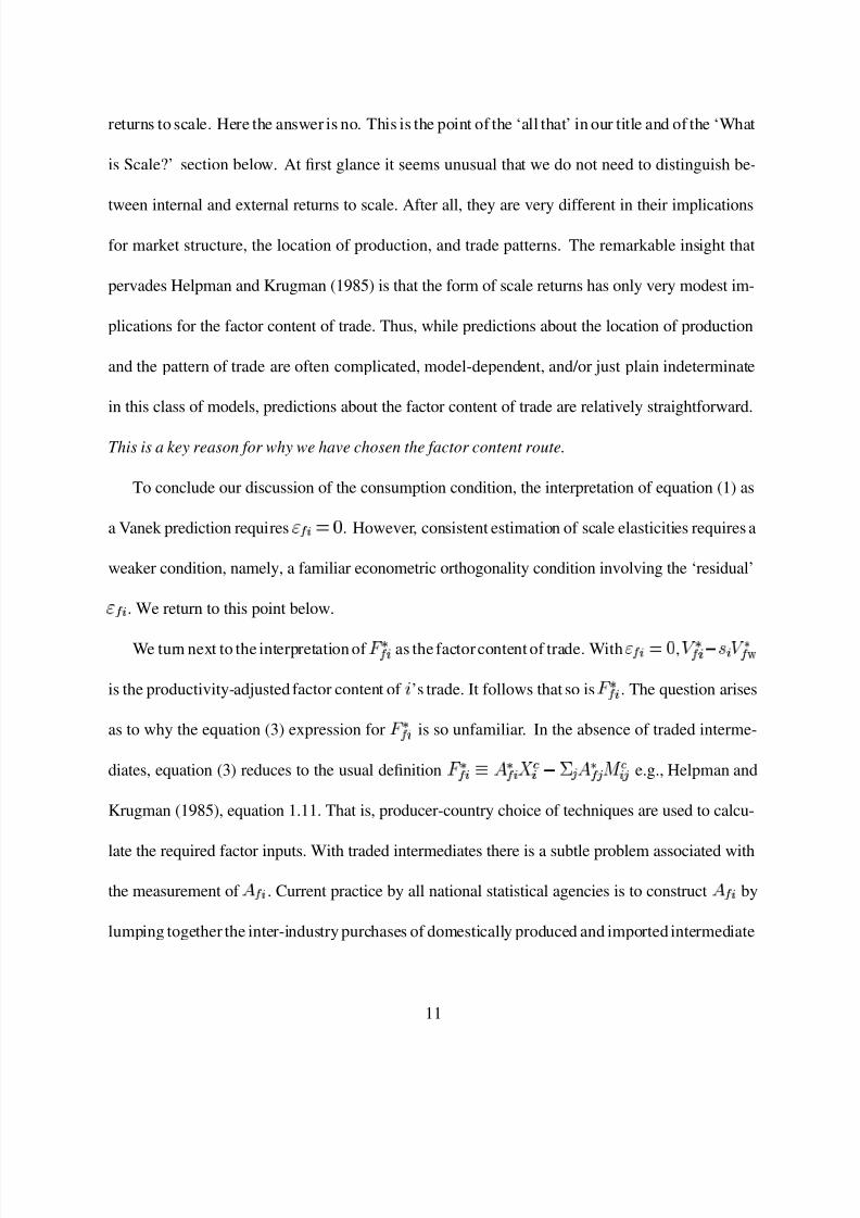
returns to scale. Here the answer is no. This is the point of the ‘all that’ in our title and of the ‘What
is Scale?’ section below. At first glance it seems unusual that we do not need to distinguish be-
tween internal and external returns to scale. After all, they are very different in their implications
for market structure, the location of production, and trade patterns. The remarkable insight that
pervades Helpman and Krugman (1985) is that the form of scale returns has only very modest im-
plications for the factor content of trade. Thus, while predictions about the location of production
and the pattern of trade are often complicated, model-dependent, and/or just plain indeterminate
in this class of models, predictions about the factor content of trade are relatively straightforward.
This is a key reason for why we have chosen the factor content route.
To conclude our discussion of the consumption condition, the interpretation of equation (1) as
a Vanek prediction requires
5
©
Q
. However, consistent estimation of scale elasticities requires a
weaker condition, namely, a familiar econometric orthogonality condition involving the ‘residual’
5
© . We return to this point below.
We turn next to the interpretation of 2
5
©
as the factorcontent of trade. With
5
©
Q
,4
5
© P
E
©
4
5 A
is the productivity-adjusted factor content of ’s trade. It follows that so is
2
5
©
. The question arises
as to why the equation (3) expression for2
5
©
is so unfamiliar. In the absence of traded interme-
diates, equation (3) reduces to the usual definition 2
5
© 9
5
©
f`
© P C
T
5
T
Y`
© T
e.g., Helpman and
Krugman (1985), equation 1.11. That is, producer-country choice of techniques are used to calcu-
late the required factor inputs. With traded intermediates there is a subtle problem associated with
the measurement of 5
© . Current practice by all national statistical agencies is to construct 5
© by
lumping together the inter-industry purchases of domestically produced and imported intermediate
11
8/3/2019 Increasing Returns and All That (Antweiler and Trefler, 2002)
http://slidepdf.com/reader/full/increasing-returns-and-all-that-antweiler-and-trefler-2002 14/59
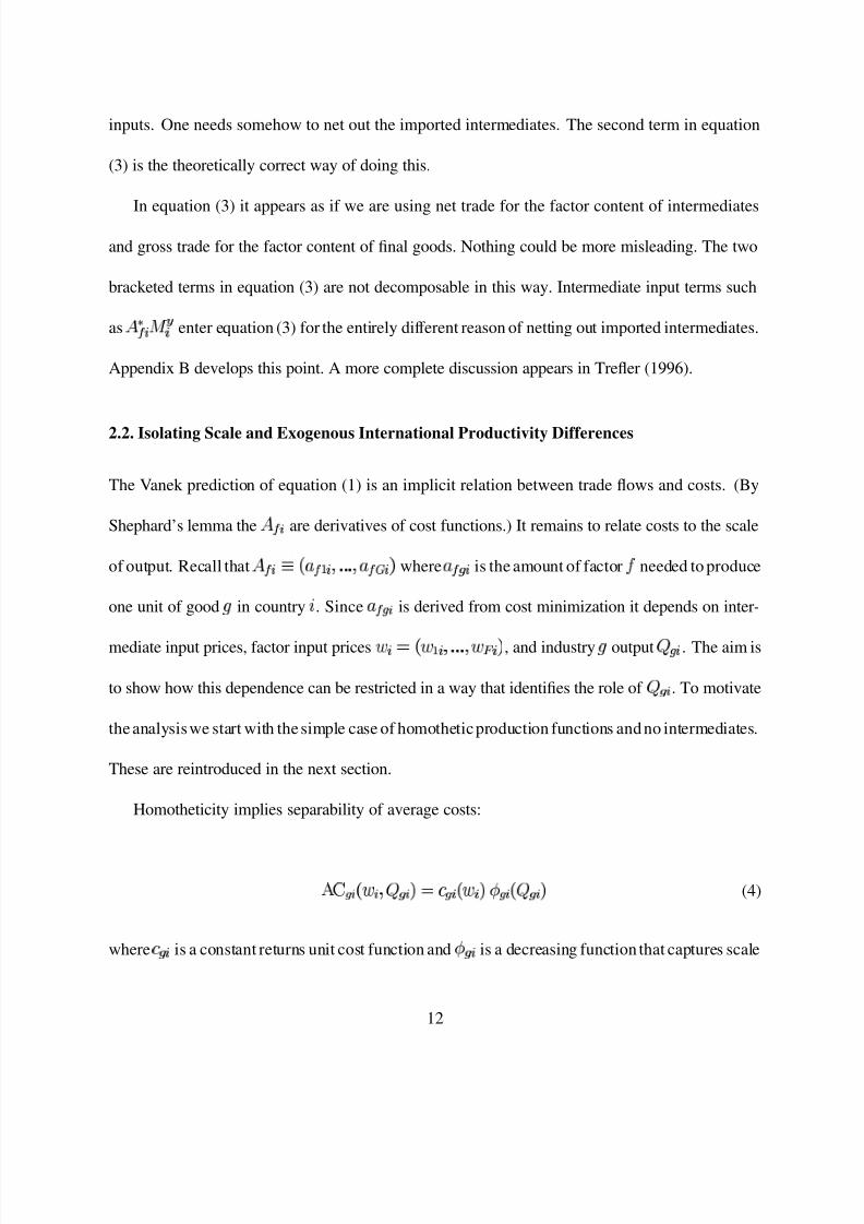
inputs. One needs somehow to net out the imported intermediates. The second term in equation
(3) is the theoretically correct way of doing this.
In equation (3) it appears as if we are using net trade for the factor content of intermediates
and gross trade for the factor content of final goods. Nothing could be more misleading. The two
bracketed terms in equation (3) are not decomposable in this way. Intermediate input terms such
as
5
©
Y r
©
enter equation (3) for the entirely different reason of netting out imported intermediates.
Appendix B develops this point. A more complete discussion appears in Trefler (1996).
2.2. Isolating Scale and Exogenous International Productivity Differences
The Vanek prediction of equation (1) is an implicit relation between trade flows and costs. (By
Shephard’s lemma the 5
© are derivatives of cost functions.) It remains to relate costs to the scale
of output. Recall that 5
©
9
5
©
" " "
5
© where
5
© is the amount of factor'
needed to produce
one unit of good
in country. Since
5
© is derived from cost minimization it depends on inter-
mediate input prices, factor input prices
©
©
" " "
© , and industry output
© . The aim is
to show how this dependence can be restricted in a way that identifies the role of
© . To motivate
the analysiswe start with the simple case of homotheticproduction functions and no intermediates.
These are reintroduced in the next section.
Homotheticity implies separability of average costs:
©
©
©
u
©
©
©
© (4)
whereu
© is a constant returns unit cost function and
© is a decreasing function that captures scale
12
8/3/2019 Increasing Returns and All That (Antweiler and Trefler, 2002)
http://slidepdf.com/reader/full/increasing-returns-and-all-that-antweiler-and-trefler-2002 15/59
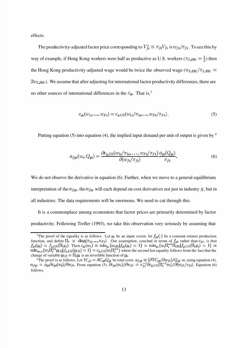
effects.
The productivity-adjusted factor price corresponding to4
5
©9
7 5
©
4 5
© is 5
©
F
7 5
© . To see this by
way of example, if Hong Kong workers were half as productive as U.S. workers (7
§
) then
the Hong Kong productivity-adjusted wage would be twice the observed wage (
F
7
). We assume that after adjusting for international factor productivity differences, there are
no other sources of international differences in the u
© . That is,3
u
©
©
" " "
©
u
¡ ¢
©
F
7
©
" " "
©
F
7
© . (5)
Putting equation (5) into equation (4), the implied input demand per unit of output is given by4
5
©
©
©
¥
u
¡ ¢
©
F
7
©
" " "
©
F
7
©
¥
5
©
F
7 5
©
©
©
7 5
©
"(6)
We do not observe the derivative in equation (6). Further, when we move to a general equilibrium
interpretation of the
5
© , the
5
© will each depend on cost derivatives not just in industry
, but in
all industries. The data requirements will be enormous. We need to cut through this.
It is a commonplace among economists that factor prices are primarily determined by factor
productivity. Following Trefler (1993), we take this observation very seriously by assuming that
3The proof of the equality is as follows. Let
be an input vector, let
{ ª
be a constant returns production
function, and define « ¬ ® ° ² ´
{ µ ¶
· ¸ ¸ ¸ ·
µ »
. Our assumption, couched in terms of
rather than ¼
, is that
{
m
½ ¾ ¿
{
«
. Then
¼
{ Á
¬ Ã ° Å Æ Ç É
Á
Ê
{
m Ë Ì m
à ° Å Æ Ç É
Á
« Í
¶
«
Ê
½ ¾ ¿
{
«
m Ë Ì m
à ° Å Æ Ï Ð É
Á
« Í
¶
¾ ¿Ê
½ ¾ ¿
{
¾ ¿
m Ë Ì m
¼ ½ ¾ ¿
{ Á
« Í
¶
where the second last equality follows from the fact that the
change of variable ¾ ¿ ¬ «
is an invertible function of
.4The proof is as follows. Let TC
m Ó Ô
be total costs. Ö± ¬
{ × Ø
Ô
Ù
× Á
Ù or, using equation (4),
Ö
m Ú
×
¼
{ Á
Ù
× Á
. From equation (5),
×
¼
{ Á
Ù
× Á
m
µ
Í
¶
×
¼ ½ ¾ ¿
{
«Í
¶
Á
Ù
× { Á
Ù
µ
. Equation (6)
follows.
13
8/3/2019 Increasing Returns and All That (Antweiler and Trefler, 2002)
http://slidepdf.com/reader/full/increasing-returns-and-all-that-antweiler-and-trefler-2002 16/59
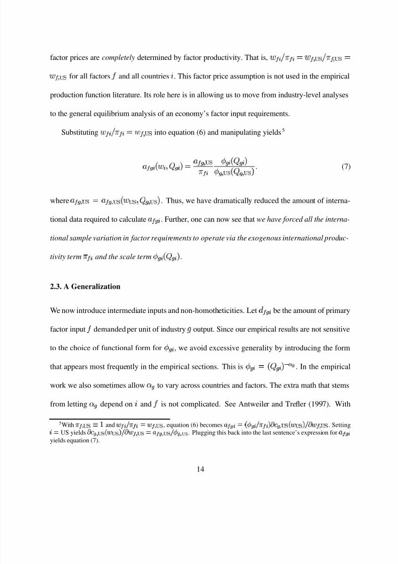
factor prices are completely determined by factor productivity. That is, 5
©
F
7 5
©
5 ¡ ¢
F
7 5 ¡ ¢
5 ¡ ¢for all factors
'and all countries
. This factor price assumption is not used in the empirical
production function literature. Its role here is in allowing us to move from industry-level analyses
to the general equilibrium analysis of an economy’s factor input requirements.
Substituting 5
©
F
7 5
©
5 ¡ ¢ into equation (6) and manipulating yields5
5
©
©
©
5
¡ ¢
7 5
©
©
©
¡ ¢
¡ ¢
. (7)
where
5
¡ ¢
5
¡ ¢
¡ ¢
¡ ¢
. Thus, we have dramatically reduced the amount of interna-
tional data required to calculate
5
© . Further, one can now see that we have forced all the interna-
tional sample variation in factor requirements to operate via the exogenous international produc-
tivity term7 5
© and the scale term
©
© .
2.3. A Generalization
We now introduce intermediate inputs and non-homotheticities. LetÜ 5
© be the amount of primary
factor input'
demanded per unit of industry
output. Since our empirical results are not sensitive
to the choice of functional form for
© , we avoid excessive generality by introducing the form
that appears most frequently in the empirical sections. This is
©
© Ý Þ ß . In the empirical
work we also sometimes allowà
to vary across countries and factors. The extra math that stems
from lettingà
depend on
and'
is not complicated. See Antweiler and Trefler (1997). With
5Withµ
½ ¾ ¿
¬
Ë andÁ
Ù
µ
m
Á
½ ¾ ¿ , equation (6) becomes Ö
m
{
Ú
Ù
µ
×
¼ ½ ¾ ¿
{ Á
¾ ¿ Ù
× Á
½ ¾ ¿ . Setting
á
m US yields×
¼ ½ ¾ ¿
{ Á
¾ ¿ Ù
× Á
½ ¾ ¿
m
Ö ½ ¾ ¿
Ù
Ú
½ US. Plugging this back into the last sentence’s expression forÖ
yields equation (7).
14
8/3/2019 Increasing Returns and All That (Antweiler and Trefler, 2002)
http://slidepdf.com/reader/full/increasing-returns-and-all-that-antweiler-and-trefler-2002 17/59
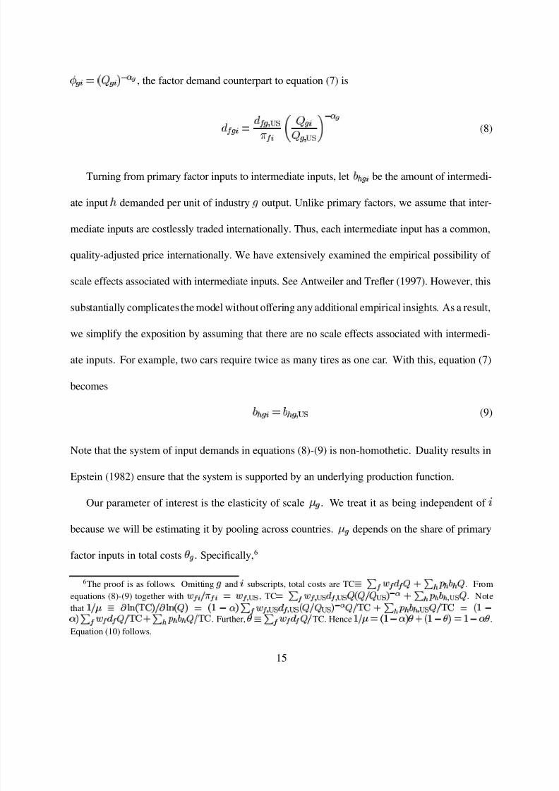
©
© Ý Þ
ß , the factor demand counterpart to equation (7) is
Ü 5
©
Ü 5
¡ ¢
7 5
©
â
©
¡ ¢ ã
Ý Þß
(8)
Turning from primary factor inputs to intermediate inputs, letä å
© be the amount of intermedi-
ate inputæ
demanded per unit of industry
output. Unlike primary factors, we assume that inter-
mediate inputs are costlessly traded internationally. Thus, each intermediate input has a common,
quality-adjusted price internationally. We have extensively examined the empirical possibility of
scale effects associated with intermediate inputs. See Antweiler and Trefler (1997). However, this
substantially complicates the model without offering any additional empirical insights. As a result,
we simplify the exposition by assuming that there are no scale effects associated with intermedi-
ate inputs. For example, two cars require twice as many tires as one car. With this, equation (7)
becomes
ä å
©
ä å
¡ ¢
(9)
Note that the system of input demands in equations (8)-(9) is non-homothetic. Duality results in
Epstein (1982) ensure that the system is supported by an underlying production function.
Our parameter of interest is the elasticity of scaleç
. We treat it as being independent of
because we will be estimating it by pooling across countries.ç
depends on the share of primary
factor inputs in total costs è
. Specifically,6
6The proof is as follows. Omitting é andá
subscripts, total costs are TC¬
¨
Á
ê ë
¨ í î
í ï í
. From
equations (8)-(9) together withÁ
Ù
µ
m
Á
½ ¾ ¿ , TC m
¨
Á
½ ¾ ¿
ê
½ ¾ ¿
{
Ù ¾ ¿
Í ð
ë
¨ í
î
íï
í
½ ¾ ¿
. Note
that Ë
Ù ñ¬
× ò
Å
{ Ø
Ô
Ù
× ò
Å
{
m
{
Ë
} ó
¨
Á
½ ¾ ¿ê
½ ¾ ¿
{
Ù ¾ ¿
Í ð
Ù
Ø
Ô
ë
¨í î
íï
í
½ ¾ ¿ Ù
Ø
Ô m
{
Ë
}
ó
¨
Á
ê
Ù
Ø
Ô
ë
¨í î
í ï í
Ù
Ø
Ô . Further,ô
¬
¨
Á
ê
ÙTC. Hence Ë
Ù ñ
m
{
Ë
} ó ô ë
{
Ë
} ô
m Ë
} ó ô.
Equation (10) follows.
15

8/3/2019 Increasing Returns and All That (Antweiler and Trefler, 2002)
http://slidepdf.com/reader/full/increasing-returns-and-all-that-antweiler-and-trefler-2002 18/59
ç
P
à
è
Ý
. (10)
With intermediate inputs,
5
© must be defined as the total factor requirements (direct plus in-
direct in an input-output sense) needed to bring one unit of good
to final consumers. In matrix
notation total factor requirements are defined in theusual input-output wayas 5
©
9 ÷
5
©
øP ù
© Ý
where÷
5
©
Ü 5
©
" " " Ü 5
© andù
© is thew x w
-matrix whose
æ
element isä å
© . We can now
state the main result of this section about how
5
©
varies with output and observed data.
Theorem 1. Input demand equations (8)-(9) imply
5
©
ç
9
7 5
©
5
©
÷
5 ¡ ¢ ü
©
¡ ¢ ý ç
øP ù
¡ ¢
Ý
(11)
where ç
9
ç " " " ç
and ü
©
¡ ¢ ý ç
is a w x w diagonal matrix whose th element is
â
©
¡ ¢ã
Ý ¢ß ¤ ¦
¢
ß ¨ ß ¤
.
The proof is straightforward.7 Theorem 1 provides a parameterization of scale effects that is con-
sistent with our general equilibrium trade theories.
7Start withµ
¹ z ¬
µ
{
}
Í
¶ . From equations (8) and (10),µ
ê1
m
ê ½ ¾ ¿
{
Ù ½ ¾ ¿
Í ð
m
ê ½ ¾ ¿
{
Ù ½ ¾ ¿
¶
Í " $
% "
. Hence,µ
m
½ ¾ ¿ ' . From equation (9),{
}
Í
¶m
{
} ¾ ¿
Í
¶ .
Hence µ
z
m
½ ¾ ¿ '
{
} ¾ ¿
Í
¶
as required.
16
8/3/2019 Increasing Returns and All That (Antweiler and Trefler, 2002)
http://slidepdf.com/reader/full/increasing-returns-and-all-that-antweiler-and-trefler-2002 19/59
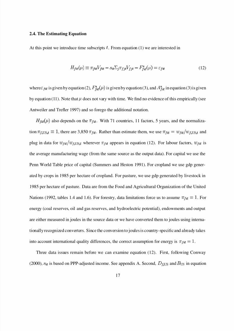
2.4. The Estimating Equation
At this point we introduce time subscripts 1 . From equation (1) we are interested in
2
5
© 3
ç
9
7 5
© 3
4 5
© 3
P
E
© 3
C
T
7 5
T 3
4 5
T 3
P
2
5
© 3
ç
5
© 3 (12)
where
5
© 3 is given by equation(2), 2
5
© 3
ç
is givenby equation(3), and
5
© 3
in equation(3) is given
by equation (11). Note thatç
does not vary with time. We find no evidence of this empirically (see
Antweiler and Trefler 1997) and so forego the additional notation.
2
5
© 3
ç
also depends on the7 5
© 3 . With 71 countries, 11 factors, 5 years, and the normaliza-
tion7 5 ¡ ¢
3
9
, there are 3,850
7 5
© 3 . Rather than estimate them, we use7 5
© 3
5
© 3
F
5 ¡ ¢
3 and
plug in data for 5
© 3
F
5 ¡ ¢
3 wherever 7 5
© 3 appears in equation (12). For labour factors, 5
© 3 is
the average manufacturing wage (from the same source as the output data). For capital we use the
Penn World Table price of capital (Summers and Heston 1991). For cropland we use gdp gener-
ated by crops in 1985 per hectare of cropland. For pasture, we use gdp generated by livestock in
1985 per hectare of pasture. Data are from the Food and Agricultural Organization of the United
Nations (1992, tables 1.4 and 1.6). For forestry, data limitations force us to assume7 5
© 3
. For
energy (coal reserves, oil and gas reserves, and hydroelectric potential), endowments and output
are either measured in joules in the source data or we have converted them to joules using interna-
tionally recognized converters. Since the conversion to joules is country-specificand already takes
into account international quality differences, the correct assumption for energy is7 5
© 3
.
Three data issues remain before we can examine equation (12). First, following Conway
(2000),E
© 3 is based on PPP-adjusted income. See appendix A. Second,÷
5 ¡ ¢and
ù
¡ ¢in equation
17

8/3/2019 Increasing Returns and All That (Antweiler and Trefler, 2002)
http://slidepdf.com/reader/full/increasing-returns-and-all-that-antweiler-and-trefler-2002 20/59
(11) andè
in equation (10) use U.S. data. The source data are described in appendix A. Third,
we need to know the share of trade that is intermediate inputs trade. For example, we observe
f `
© 3
fr
© 3
, but notf `
© 3
orf
r
© 3
separately. Appendix C details our method for allocating trade into
its intermediate and final goods components. We were initially concerned that our estimates of ç
would be sensitive to our allocationmethod. This turns out to be a misplaced concern. To persuade
the reader of this, appendixC also reports estimates of scale for many different allocation methods.
We summarize by noting some differences between our general equilibrium approach and ex-
isting partial equilibrium approaches to estimating scale returns in a cross-country setting. On the
input side, data on industry-level inputs are notoriously bad or non-existent e.g., labour inputs by
educational attainment. While partial equilibrium approaches must use such data, our approach al-
lows us to use national-level aggregates. These aggregates are typically more reliable. In addition,
our approacheasily allows us to model international differences in input productivities i.e., the7 5
© .
On the output side, we are able to shift some of the burden off of gross output data and onto trade
flow data. Real gross output data suffer a number of serious problems, especially for poorer coun-
tries. In contrast, trade flow data are more accurate, measured in dollars, and with the approximate
assumption of equal prices across countries, correspondmore directly to physical quantities. Thus,
the general equilibrium approach allows us to exploit alternative and somewhat more reliable data
sources.
18

8/3/2019 Increasing Returns and All That (Antweiler and Trefler, 2002)
http://slidepdf.com/reader/full/increasing-returns-and-all-that-antweiler-and-trefler-2002 21/59
3. Results
We re-write equation (12) as our final estimating equation
2
5
© 3
ç
7
5
© 3
8
©
@
5
© 3 (13)
where the following holds.2
5
© 3
ç
is defined in equation (12). The 7
5
© 3 are generalized least
squares (GLS) corrections with factor-year and country-year components. Appendix D describes
the 7
5
© 3 in detail.
5
© 3 of equations (2) and (12) is now written as the sum of two components,
5
© 3
F
7
5
© 3
8
©
@
5
© 3 . The 8
© are country fixed effects and the@
5
© 3 are independently and identically
distributed disturbances with mean zero. We estimate equation (13) using maximum likelihood
(ML), non-linear least squares (NLS), and non-linear two-stage least-squares (NL2SLS) estima-
tors. These are reviewed in the next section.
3.1. Preliminary Estimation
To fix ideas about the specification we start with the strong assumption that all industries exhibit
the same degree of scale economies. We will relax this shortly. We pool across all 71 countries, all
11 factors, and all 5 years to give us B C
Q D
observations. The 5 years are 1972, 1977, 1982, 1987,
and 1992.
Table 2 reports the estimated scale elasticities for a variety of estimators. We start with the ML
and NLS estimators. They are distinguished by their use of exogeneity assumptions. In general
equilibrium almost everything is endogenous including endowments of physical and human capi-
19
8/3/2019 Increasing Returns and All That (Antweiler and Trefler, 2002)
http://slidepdf.com/reader/full/increasing-returns-and-all-that-antweiler-and-trefler-2002 22/59
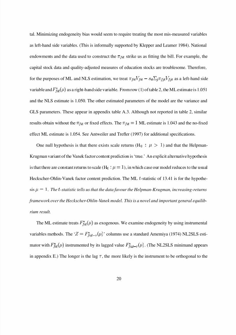
tal. Minimizing endogeneity bias would seem to require treating the most mis-measured variables
as left-hand side variables. (This is informally supported by Klepper and Leamer 1984). National
endowments and the data used to construct the7 5
© 3
strike us as fitting the bill. For example, the
capital stock data and quality-adjusted measures of education stocks are troublesome. Therefore,
for the purposes of ML and NLS estimation, we treat 7 5
© 3
4 5
© 3
P
E
© 3
C
T
7 5
T 3
4 5
T 3 as a left-hand side
variableand 2
5
© 3
ç
as a right-handside variable. Fromrow (1) of table 2, the ML estimate is 1.051
and the NLS estimate is 1.050. The other estimated parameters of the model are the variance and
GLS parameters. These appear in appendix table A.3. Although not reported in table 2, similar
results obtain without the7 5
© 3 or fixed effects. The7 5
© 3
ML estimate is 1.043 and the no-fixed
effect ML estimate is 1.054. See Antweiler and Trefler (1997) for additional specifications.
One null hypothesis is that there exists scale returns (H GH ç
H
) and that the Helpman-
Krugman variant of the Vanek factorcontent prediction is ‘true.’ An explicit alternative hypothesis
is that there are constant returns to scale (HGH ç
), in which case our model reduces to the usual
Heckscher-Ohlin-Vanek factor content prediction. The ML 1 -statistic of 13.41 is for the hypothe-
sisç
. The 1 -statistic tells us that the data favour the Helpman-Krugman, increasing-returns
framework over the Heckscher-Ohlin-Vanek model. This is a novel and important general equilib-
rium result.
The ML estimate treats 2
5
© 3
ç
as exogenous. We examine endogeneity by using instrumental
variables methods. The ‘Q
2
5
©
3
Ý R
ç
’ columns use a standard Amemiya (1974) NL2SLS esti-
mator with2
5
© 3
ç
instrumented by its lagged value2
5
©
3
Ý R
ç
. (The NL2SLS minimand appears
in appendix E.) The longer is the lag S , the more likely is the instrument to be orthogonal to the
20
8/3/2019 Increasing Returns and All That (Antweiler and Trefler, 2002)
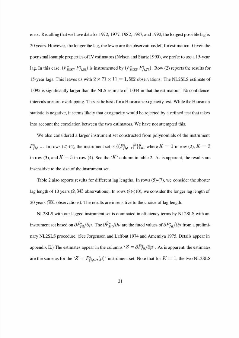
http://slidepdf.com/reader/full/increasing-returns-and-all-that-antweiler-and-trefler-2002 23/59
error. Recalling that we have data for 1972, 1977, 1982, 1987, and 1992, the longest possible lag is
20 years. However, the longer the lag, the fewer are the observations left for estimation. Given the
poor small-sample properties of IV estimators (Nelson and Startz 1990), we prefer to use a 15-year
lag. In this case,
2
5
©
T
U
2
5
©
V
§
is instrumented by
2
5
©
U
§
2
5
©
U
U
. Row (2) reports the results for
15-year lags. This leaves us with
xW
x
DY
observations. The NL2SLS estimate of
1.095 is significantly larger than the NLS estimate of 1.044 in that the estimators’ 1% confidence
intervals arenon-overlapping. This is thebasis for a Hausman exogeneity test. While the Hausman
statistic is negative, it seems likely that exogeneity would be rejected by a refined test that takes
into account the correlation between the two estimators. We have not attempted this.
We also considered a larger instrument set constructed from polynomials of the instrument
2
5
©
3
Ý R
. In rows (2)-(4), the instrument set is a
2
5
©
3
Ý R
b c e
b
p
where f in row (2), f
B
in row (3), and f
D
in row (4). See the ‘ f ’ column in table 2. As is apparent, the results are
insensitive to the size of the instrument set.
Table 2 also reports results for different lag lengths. In rows (5)-(7), we consider the shorter
lag length of 10 years (
B i Bobservations). In rows (8)-(10), we consider the longer lag length of
20 years ( Wp
observations). The results are insensitive to the choice of lag length.
NL2SLS with our lagged instrument set is dominated in efficiency terms by NL2SLS with an
instrument set based on¥
q
2
5
© 3 F
¥
ç . The¥
q
2
5
© 3 F
¥
ç are the fitted values of ¥
2
5
© 3 F
¥
ç from a prelimi-
nary NL2SLS procedure. (See Jorgenson and Laffont 1974 and Amemiya 1975. Details appear in
appendix E.) The estimates appear in the columns ‘ Q
¥
q
2
5
© 3 F
¥
ç’. As is apparent, the estimates
are the same as for the ‘ Q 2
5
©
3
Ý R
ç
’ instrument set. Note that for f
, the two NL2SLS
21
8/3/2019 Increasing Returns and All That (Antweiler and Trefler, 2002)
http://slidepdf.com/reader/full/increasing-returns-and-all-that-antweiler-and-trefler-2002 24/59
estimates are mathematically equivalent.
The bottom line from table 2 is that there is evidence of modest scale economies at the aggre-
gate level no matter how one tackles estimation. The elasticity estimate of 1.051 is well within the
bounds of what has been reported in the U.S. time series literature (e.g., Basu 1995 and Basu and
Fernald 1997). Against our conclusion of statistically significant scale returns must be weighed the
economically small size of the estimated ç . A 1% rise in output is associated with a 0.05% fall in
average costs. Further, a country operating at a tenth of U.S. levels has only 14% higher average
costs.8 Of course, in dynamic models such as those displaying endogenous growth and especially
hysteresis,ç "
Q D
can have important consequences.
The factor demand implications of ç "
Q D
are much larger than the average cost impli-
cations. From equation (8), the elasticity of factor demand per unit of output is à . From the last
footnote,ç "
Q D
implies
à
Q
" p. That is, a 1% rise in output leads to a 0.18% fall in demand
for primary inputs per unit of output. Further, a country operating at a tenth of U.S. output levels
uses 51%
"
Q
Ý s
T
P
more productivity-adjusted factor inputs per unit of output. Thus, from
the perspective of factor endowments theory even this small scale estimate is very important. We
will see that it has some implications for the ‘mystery of missing trade’ (Trefler 1995).
8Dropping é andá
subscripts, 0.05% follows from the fact that× ò
ÅAC Ù
× ò
Å
m
× ò
ÅTC Ù
× ò
Å }
Ë m Ë
Ù ñ }
Ë m
}
¸
u . 14% is calculated as follows. From AC{
m v
Á
ê ë
v
í
î
í ï í and equations (8)-(9), AC{
m
{
Ù ¾ ¿
Í ð
v
Á
½ ¾ ¿
ê ½ ¾ ¿ ë
v
í
î
í ï í
½ ¾ ¿ . Using ô ¾ ¿
m v
Á
½ ¾ ¿
ê ½ ¾ ¿ Ù AC
{
¾ ¿ yields AC{
Ù AC{
¾ ¿
m
{
Ù ¾ ¿
Í ð
ô ë
{
Ë
} ô . With
ô
m
¸y
(see appendix A) and
ñ
m Ë
¸
u Ë , equation (10) impliesó
m
¸
Ë . Hence
AC{
Ù AC{
¾ ¿
m Ë
¸
Ë
.
22

8/3/2019 Increasing Returns and All That (Antweiler and Trefler, 2002)
http://slidepdf.com/reader/full/increasing-returns-and-all-that-antweiler-and-trefler-2002 25/59
3.2. Industry-Level Analysis
General equilibrium estimation is complicated. We have found it computationally infeasible to
simultaneously estimate separate scale elasticities for all 34 industries. Fortunately, there are other
paths to interesting results. Consider the following iterative three-step procedure:
1. Rank industries by the size of their scale elasticities. In thefirst iteration this ranking is based
on external information. In subsequent iterations it is taken from the output of the previous
iteration.
2. Pick a particular industry, place all industries higher in the ranking in one group and all
industries lower in the ranking in another group. Industry
sits in a separate, third group.
Use ML to estimate equation (13) subject to the restriction that all industries within a group
share a common scale elasticity. This yields scale estimatesq
ç
,q
ç
, andq
ç
for the
high, low, and
groups, respectively.9
3. Repeat step 2 for each. This yields a set of scale estimates a
q
ç
c
p
. Return to step 1
using a
q
ç
c
p
to rank industries.
Since thechoice of initial rank does not matter, we deferdescriptionof this choice to the‘Sensitivity
Analysis’ section. In that section we also note that there are no algorithm convergence issues.
Table 3 reports theq
ç
for the specification with 71 countries, 11 factors, and 5 years. In the
table industries are classified into four groups. The increasing returns to scale (IRS) group contains
those industries withq
ç
that are significantly greater than unity at the 1% level. (Instruments is
9Since the lowest ranked industry can never be in theé
group, its elasticity is given byñ
for the case where
both the low and é groups each have only 1 industry. A similar detail applies to the highest ranked industry.
23
8/3/2019 Increasing Returns and All That (Antweiler and Trefler, 2002)
http://slidepdf.com/reader/full/increasing-returns-and-all-that-antweiler-and-trefler-2002 26/59
an exception, but we include it because it is significant in every other specification examined in
the ‘Sensitivity Analysis’ section.) We distinguish between manufacturing and natural resources
because the natural resource scale estimates may reflect not only scale, but also Heckscher-Ohlin
misspecification. Theconstantreturns to scale (CRS) group containsthose industries withq
ç
that
are insignificantly different from unity at the 1% level. In a few cases, such as electricity where
q
ç
"
Q
i and 1
Q
"
Y
W , being in the CRS group really means that scale returns are imprecisely
estimated. The ‘Non-Robust’ group collects industries for which scale is not robustly estimated.
Robustness will be made precise in the ‘Sensitivity Section’ section below.
Table 3 shows a number of striking patterns. First, the constant returns to scale industries are
all sensible. These include Apparel, Leather, and Footwear. Second, the industries estimated to
display scale returns are also all sensible. These include Pharmaceuticals, Electric and Electronic
Machinery, and Non-Electrical Machinery.
To get a handle on magnitudes, consider a scale elasticity of 1.15. This implies that a 1% rise
in output leads to a 0.13% fall in average cost. Further, a country operating at a tenth of U.S. levels
faces 55% higher average costs. These are large numbers.
How do our results compare to existing partial equilibrium production function-based esti-
mates? Tybout (2000) surveyed studies for many developing countries and found little evidence
of scale returns. This is a key finding. He partly attributed it to the fact that “small firms in de-
veloping countries tend not to locate in those industries where they would be at substantial cost
disadvantage relative to larger incumbents” (Tybout 2000, page 19). This squares readily with our
finding of constant returns to scale in all low-end manufacturing industries. The evidence of scale
24
8/3/2019 Increasing Returns and All That (Antweiler and Trefler, 2002)
http://slidepdf.com/reader/full/increasing-returns-and-all-that-antweiler-and-trefler-2002 27/59
from middle-income countries is less clear cut. Using Chilean plant-level data for 8 industries,
Levinsohn and Petrin (1999) estimated scale returns from value-added production functions that
are never less than 1.20 and reach as high 1.44. Using Mexican plant-level data, Tybout and West-
brook (1995) obtained almost no evidence of scale for large plants. It is not immediately clear
that our results are inconsistent with Tybout and Westbrook: we find constant returns for many in-
dustries and increasing returns primarily for industries not examined by them. For rich countries,
Harrigan (1999) found no evidence of scale in cross-country regressions. However, many other
OECD country studies point clearly to the existence of scale returns. Paul and Siegel (1999) es-
timated industry-level scale returns in the range of 1.30 for many U.S. manufacturing industries.
Estimates closer to our mode of 1.15 are common in OECD studies e.g., Fuss and Gupta (1981)
for Canada and Griliches and Ringstad (1971) for Norway. Thus, our general equilibrium results
are consistent with some, though not all of the existing partial equilibrium benchmarks.
3.3. Grouped Results
A drawback to the approach of the last section is that we did not simultaneously estimate each
industry’s scale elasticity. The estimation algorithm is only partially simultaneous. Further, we
did not deal with endogeneity. To address these issues we follow table 3 in classifying industries
into three groups: IRS, CRS, and Non-Robust.10 We then estimate the model under the assumption
that scale elasticities are the same within each group, but different between groups. Note that the
IRS group includes both manufacturing and natural resource-based IRS industries. Disaggregation
10Theclassification of industries into these 3 groups is slightly different from that reported in table 3. This is a minor
point; however, we cannot properly explain it until after we have laid out the criteria for being in the ‘Non-Robust’
group. See the ‘Sensitivity Analysis’ section below.
25
8/3/2019 Increasing Returns and All That (Antweiler and Trefler, 2002)
http://slidepdf.com/reader/full/increasing-returns-and-all-that-antweiler-and-trefler-2002 28/59
of the IRS group into manufacturing and natural resources adds little to the analysis.
The top panel of table 4 reports the results for the usual specification with 71 countries and 11
factors. The NL2SLS estimator uses the preferred instrument set from row 3 of table 2. That is, it
uses the2
5
©
3
Ý R
ç
instrument set with a f B
polynomial order and a 15-year lag length. This
leaves us with only the years 1987 and 1992. We do not report any of the other specifications that
appeared in table 2 since this would be too repetitive. Instead, we report the results for the sample
consisting only of our 23 OECD members. (See table A.1 for a list of these countries and the end
of appendix A for a discussion of how the world is defined with 23 countries.) From the bottom
panel of table 4, the 23-country results are very similar to the 71-country results, though somewhat
less significant. The reduced significance arises from having eliminated an important source of
sample variation, namely, trade with non-OECD countries such as Hong Kong and Singapore. For
23 countries, the Hausman
§
test statistic of 490 strongly supports the hypothesis of endogeneity.
The conclusions from table 4 are clear. The IRS group is always estimated to have significant
scale returns. As in table 2, the NL2SLS estimate is larger than its ML counterpart which assume
exogeneity. The CRS group is always estimated to have a scale elasticity that is insignificantly
different from unity. For the Non-Robust group, almost by definition, the conclusion depends on
theestimation method. Overall, the table 4 results are whollyconsistent with theestimatesreported
in tables 2-3. By implication we must abandon empirical models that treat all industries as if they
were subject exclusively to either constant or increasing returns. Both play an important role for
understanding the sources of comparative advantage.
26
8/3/2019 Increasing Returns and All That (Antweiler and Trefler, 2002)
http://slidepdf.com/reader/full/increasing-returns-and-all-that-antweiler-and-trefler-2002 29/59
3.4. What is Scale?
As discussed in the introduction, we are using scale (and ‘all that’) to mean something more than
just plant-level economies. For one, scale likely includes industry-level externalities. By way of
example, growth of the Petroleum Refining industry was accompanied by the development of a
host of specialized inputs including specialized engineering firms, industry-sponsored institutes,
and specialized machinery manufacturers. Paul and Siegel (1999) argued that more than half of
the relationship between cost and scale in U.S. manufacturing is due to such industry-level exter-
nalities. To the extent that this holds worldwide, it implies that a portion of what we are calling
‘scale’ is actually industry-level externalities.
Also, scale likely includes aspects of dynamic international technology differences. In table 3,
the industries with the largest scale estimates are often those where technical change has been most
rapid e.g., Pharmaceuticals. New goods often engender new process technologies and these new
process technologies are often embodied in larger plants. As Rosenberg (1982, 1994) has tirelessly
argued:
“In this respect it is much more commonthan it ought to be to assume that the exploita-
tion of the benefits of large-scale production is a separate phenomenon independent of
technological change. In fact, larger plants typically incorporate a number of techno-
logical improvements ...” (Rosenberg 1994, page 199)
While it is important conceptually to distinguish between scale and dynamic technical change, the
fact that technical change is the hand maiden of scale makes this distinction empirically problem-
atic. Even with the unusually detailed McKinsey data, Baily and Gersbach (1995) were forced
to lump international technology differences together with scale as inseparable sources of global
27
8/3/2019 Increasing Returns and All That (Antweiler and Trefler, 2002)
http://slidepdf.com/reader/full/increasing-returns-and-all-that-antweiler-and-trefler-2002 30/59
competition. In short, for the most dynamic industries, available data do not allow us to distinguish
between scale and scale-biased technical change. This is a critical area for future research.
Is it possible that our scale estimates also capture more traditional or static international tech-
nology differences? At the most obvious level the answer is no. Our7 5
© explicitly capture the
most important static international technology differences. A more subtle approach to answering
the question is as follows. Suppose that country is particularly efficient at producing a good in
the sense of having a large ratio of output to employment. By Ricardian comparative advantage,
the country will expand output of the industry. Looking across countries for a single industry, the
larger is the level of industry output, the larger is the ratio of output to employment. The careless
researcher will incorrectly attribute this correlation to increasing returns to scale. Obviously we
have not been careless. However, to dispel any possible confusion we make the following obser-
vations.
The first observation draws on an analogy between our general equilibrium econometric work
and the econometrics of production functions.11 Static international technology differences can
be thought of as unobserved productivity shocks that effect decisions about both inputs and out-
puts. They therefore induce endogeneity bias in regressions of output on inputs (e.g., Griliches and
Mairesse 1995). The techniques commonly used to control for unobserved productivity shocks
are fixed effects and IV estimators. These are exactly the econometric techniques we have used
throughout this paper. These techniques provided no evidence that our scale estimates are arti-
11We hasten to add that the analogy with partial equilibrium production function estimation only goes so far. In our
general equilibrium setting, observations have a factor dimension and data from all industries enter into each obser-
vation. See equation (13).
28
8/3/2019 Increasing Returns and All That (Antweiler and Trefler, 2002)
http://slidepdf.com/reader/full/increasing-returns-and-all-that-antweiler-and-trefler-2002 31/59
facts of unobserved international productivity differences.12
The second observation about the correct interpretation of our results comes from the cross-
industry distribution of our scale estimates. In the Ricardian interpretation, all relatively low-cost
producers are large producers. That is, static international technology differences will masquerade
as scale effects in all industries, be it Pharmaceuticals or Apparel. If so, we should have estimated
significant scale effects in every industry. We found nothing of the sort. To the contrary, we found
strong evidence of constant returns to scale in many industries e.g., Apparel. We thus find the Ri-
cardian interpretation untenable.
To summarize this section, our scale estimates likely capture plant-level scale, industry-level
externalities, and scale-biasedtechnical change. However, the idea that our estimates of increasing
returns to scale are really static international technology differences in disguise has about as much
life in it as old Ricardo himself.
4. Sensitivity Analysis
In assigning industries to the IRS and CRS groups, we have been using a stringent set of criteria:
the inference of increasing or constant returns was required to be robust across a wide variety of
specifications. Industries thatdid notmeetthe criteriawereunceremoniouslydumpedinto the Non-
Robust group. This section reviews the sensitivity analysis underlying our robustness criteria. In
12To the contrary, the IV estimates were sometimes larger than the ML estimates. This IV-ML ranking deserves
further consideration. In a production function setting, endogeneity bias is usually taken to mean that the coefficient
on labour is upward-biased and the coefficient on less variable inputs such as capital are downward biased (Olley and
Pakes 1996). It need not imply that the sum of the coefficients (i.e., the scale elasticity) is upward biased. Indeed,
Levinsohn and Petrin (1999) found that a modified Olley-Pakes solution to endogeneity bias raises the estimate of
scale in 3 of 8 Chilean industries examined. Thus, there is nothing terribly unusual about our IV-ML ranking.
29

8/3/2019 Increasing Returns and All That (Antweiler and Trefler, 2002)
http://slidepdf.com/reader/full/increasing-returns-and-all-that-antweiler-and-trefler-2002 32/59
the interests of space, the discussion is terse.
There are three issues to be clarified before robustness can be fully defined. The first deals with
whether the results depend on the initial ranking of industries used to kick off the section 3.2 esti-
mation algorithm. Consider table 5. Results in the ‘Initial Rank: Baseline’ column with 71 coun-
tries and 11 factors reproduce the table 3 results. A single asterisk indicates thatq
ç
is greater
than unity at the 1% level, two asterisks indicate 1
H D
and three asterisks indicate 1
H
Q
. The
baseline initial rank uses an initial ranking that is an average of industries’ capital-intensity and
skill-intensity ranks. See the last column of table 1. Results in the ‘Initial Rank: Alternative’ col-
umn use an initial ranking based on the scale parameters reported in Paul and Siegel (1999).13 The
baseline and alternative initial ranks are very different. The correlation is only 0.13. It is therefore
re-assuring that the scale estimates produced by the two initial ranks are almost identical. That is,
the table 3 results are insensitive to the initial ranking.
The second robustness issue deals with parameter stability across a variety of specifications.
Table 3 reports results for the specification with 71 countries, 11 factors, and 5 years. For robust-
ness, we require similar results from a specification using only the 23 OECD countries in our sam-
ple. We also require similar results from a specification that places more weight on capital and
labour and less weight on land and energy i.e., a specification with 7 factors (aggregate land, ag-
gregate energy, capital, and 4 types of labour). The last two columns of table 5 provide the scale
estimates for these two specifications.
13Paul and Siegel (1999) work at a higher level of aggregation (19manufacturing industries). We thereforerepeated
their scale elasticity values at the disaggregated level (27 manufacturing industries) where necessary. For industries
not covered by Paul and Siegel (7 non-manufacturing industries), we set the scale elasticities to unity. In the case of
ties we used information from the baseline initial rank.
30

8/3/2019 Increasing Returns and All That (Antweiler and Trefler, 2002)
http://slidepdf.com/reader/full/increasing-returns-and-all-that-antweiler-and-trefler-2002 33/59
Looking across the four table 4 specifications, the following emerges. There is considerable
stability across specifications for the ‘IRS - Manufacturing’ industries and somewhat less stability
for the ‘IRS - Natural Resources’ industries. The least amount of stability is for the ‘Non-Robust’
category. It is composed of industries that display significant increasing returns in one specifica-
tion and constant returns in another. By definition, the Non-Robust group displays the greatest
instability. Table 5 over-represents instability by omitting the CRS industries listed in table 3. By
definition of the CRS group, its member industries always display constant returns (insignificant
q
ç
). Hence scale estimates for this group are very stable across specifications.
Before turning to our last robustness issue we will need to comment on the convergence of
our section 3.2 algorithm. All the results reported in this paper are based on 10 iterations of the
algorithm. To examine convergence, at least for the table 3 specification, we allowed the algorithm
to runtheextra twoweeksneeded to complete 20 iterations. The results were unchanged from those
reported in table 3. Thus, we have restricted ourselves to 10 iterations of the algorithm.
The third and last robustness issue arises from the fact that the estimation algorithm converges
to a cycling pattern for some industries. For example, in the baseline initial rank specification with
71 countries and 11 factors, the Basic Chemicals and Plastic Products industries either both display
increasing returns (as in odd iterations of our algorithm) or both display constant returns (as in even
iterations). Cycling could never happen in traditional industry-by-industryproduction function es-
timation and captures in an obvious way the fact that we are estimating scale returns in a general
equilibrium setting. In tables 3 and 5, the cycling industries are added to the Non-Robust group.
In the absence of cycling it does not matter whether we report the 9 1æ
or 10 1æ
iterations. Thus, for
31
8/3/2019 Increasing Returns and All That (Antweiler and Trefler, 2002)
http://slidepdf.com/reader/full/increasing-returns-and-all-that-antweiler-and-trefler-2002 34/59
the IRS category we only report the 10 1æ
iteration. For those Non-Robust industries that cycle, it
does matter which iteration we report. In order to keep the table manageable, for the Non-Robust
group we report the average value of
q
ç
across the 91
æ
and 101
æ
iterations.
The classification of industries is based on robustness across specifications. However, for a
given specification some of the Non-Robust industries properly belong in the CRS or IRS groups.
In table 5, these CRS and IRS industries are indicated by the absence of an entry and by a , re-
spectively. These Non-Robust industries are classified accordingly in table 4. For example, in the
table 4 specification with 71 countries, Furniture and Fixtures is included in the CRS group.
We can now explain exactly how industries are classified. For each industry consider the 8
estimates of ç
that come from4 specifications (the 4 columnheadings in table 5) and 2 iterations
of our algorithm (the 9 1æ and 10 1
æ iterations). If all 8 of theseq
ç
are insignificant at the 1%
level then the industry is classified as CRS. If all 8 of theseq
ç
always exceed unity and do so
significantly at least once, then the industry is classified as IRS. If the industry fails to meet either
criteria then it is classified as Non-Robust.14 This scheme ensures that only the most robust results
appear in the CRS and IRS groups.
To conclude, table 5 pointedly illustrates two important features of our work. First, for about
a third of all industries, the data are simply not informative about scale economies. These are the
industries that appear in the Non-Robust group. Second, our criteria for classifying an industry as
CRS or IRS is that the inference about scale is the same across many different specifications. For
14This classification criterion is for manufacturing industries. For natural resource-based industries the criterion is
the same except that we omit from consideration the specification with 71 countries and 7 factors. With energy and
land endowments so heavily aggregated, the 7-factor data convey very little information about natural resource-based
industries. This can be seen from table 5.
32
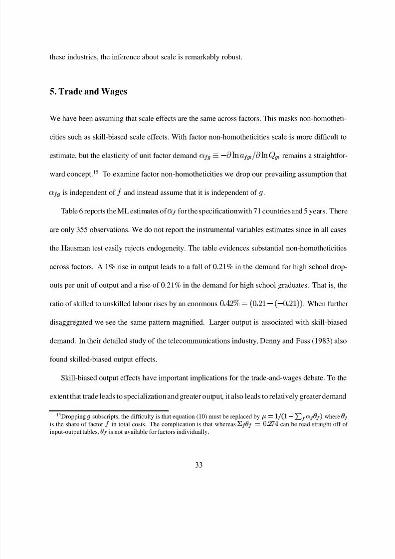
8/3/2019 Increasing Returns and All That (Antweiler and Trefler, 2002)
http://slidepdf.com/reader/full/increasing-returns-and-all-that-antweiler-and-trefler-2002 35/59
these industries, the inference about scale is remarkably robust.
5. Trade and Wages
We have been assuming that scale effects are the same across factors. This masks non-homotheti-
cities such as skill-biased scale effects. With factor non-homotheticities scale is more difficult to
estimate, but the elasticity of unit factor demandà 5
9 P
¥
5
©
F
¥
© remains a straightfor-
ward concept.15 To examine factor non-homotheticities we drop our prevailing assumption that
à 5
is independent of '
and instead assume that it is independent of
.
Table 6 reports theML estimates of à 5 for thespecificationwith 71 countriesand 5 years. There
are only 355 observations. We do not report the instrumental variables estimates since in all cases
the Hausman test easily rejects endogeneity. The table evidences substantial non-homotheticities
across factors. A 1% rise in output leads to a fall of 0.21% in the demand for high school drop-
outs per unit of output and a rise of 0.21% in the demand for high school graduates. That is, the
ratio of skilled to unskilled labour rises by an enormousQ
" i
k
Q
"
P
P
Q
"
. When further
disaggregated we see the same pattern magnified. Larger output is associated with skill-biased
demand. In their detailed study of the telecommunications industry, Denny and Fuss (1983) also
found skilled-biased output effects.
Skill-biased output effects have important implications for the trade-and-wages debate. To the
extent that trade leads to specializationand greater output, it also leads to relatively greater demand
15Droppingé
subscripts, the difficulty is that equation (10) must be replaced byñ
m Ë
Ù
{
Ë
}
¨
ó
ô
where
ô
is the share of factor
in total costs. The complication is that whereas v
ô
m
¸ y can be read straight off of
input-output tables,ô
is not available for factors individually.
33
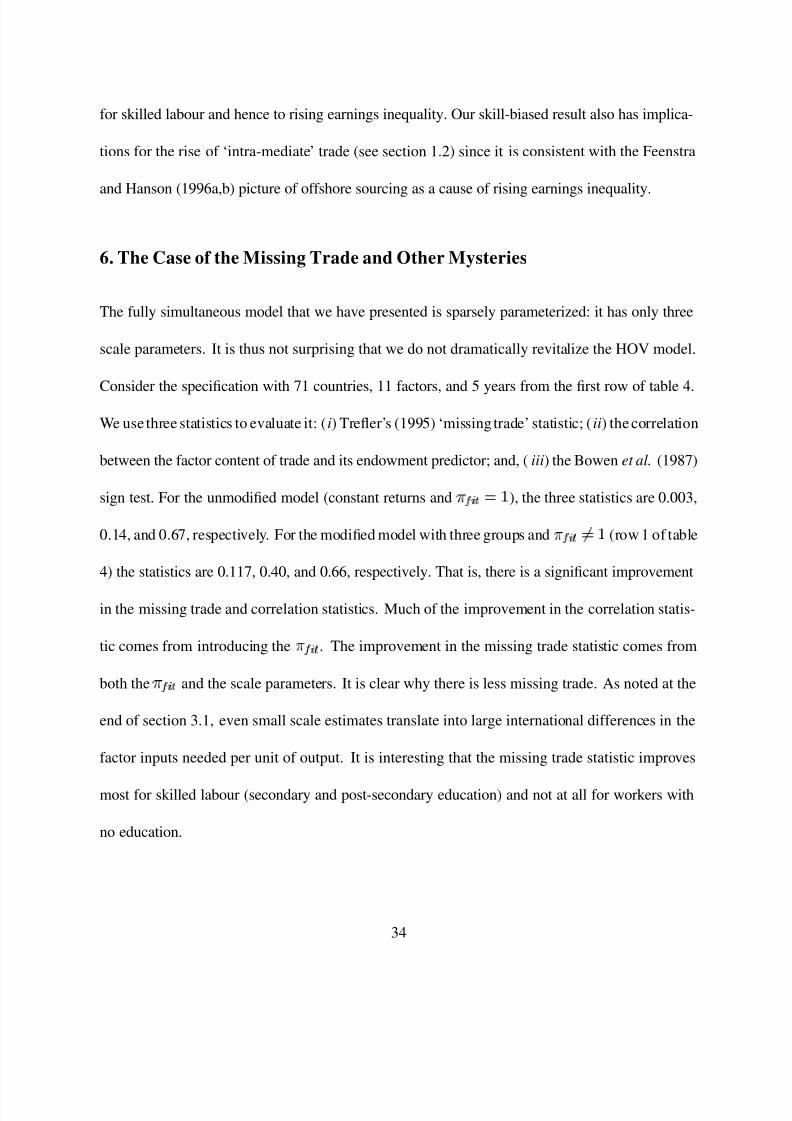
8/3/2019 Increasing Returns and All That (Antweiler and Trefler, 2002)
http://slidepdf.com/reader/full/increasing-returns-and-all-that-antweiler-and-trefler-2002 36/59
for skilled labour and hence to rising earnings inequality. Our skill-biased result also has implica-
tions for the rise of ‘intra-mediate’ trade (see section 1.2) since it is consistent with the Feenstra
and Hanson (1996a,b) picture of offshore sourcing as a cause of rising earnings inequality.
6. The Case of the Missing Trade and Other Mysteries
The fully simultaneous model that we have presented is sparsely parameterized: it has only three
scale parameters. It is thus not surprising that we do not dramatically revitalize the HOV model.
Consider the specification with 71 countries, 11 factors, and 5 years from the first row of table 4.
We use three statistics to evaluate it: (i) Trefler’s (1995) ‘missing trade’ statistic; (ii) the correlation
between the factor content of trade and its endowment predictor; and, (iii) the Bowen et al. (1987)
sign test. For the unmodified model (constant returns and 7 5
© 3
), the three statistics are 0.003,
0.14, and 0.67, respectively. For the modified model with three groups and7 5
© 3
b (row 1 of table
4) the statistics are 0.117, 0.40, and 0.66, respectively. That is, there is a significant improvement
in the missing trade and correlation statistics. Much of the improvement in the correlation statis-
tic comes from introducing the7 5
© 3 . The improvement in the missing trade statistic comes from
both the 7 5
© 3 and the scale parameters. It is clear why there is less missing trade. As noted at the
end of section 3.1, even small scale estimates translate into large international differences in the
factor inputs needed per unit of output. It is interesting that the missing trade statistic improves
most for skilled labour (secondary and post-secondary education) and not at all for workers with
no education.
34

8/3/2019 Increasing Returns and All That (Antweiler and Trefler, 2002)
http://slidepdf.com/reader/full/increasing-returns-and-all-that-antweiler-and-trefler-2002 37/59
7. Conclusions
Do scale economies contribute to our understanding of the factor content of trade? To answer
this question we examined Helpman and Krugman’s variant of the Vanek factor content prediction.
The prediction is particularly interesting in that it arises from a large class of general equilibrium,
increasing returns to scale models. To examine the prediction, we proposed an estimating equation
that is tightly allied to the theory. Theequationembodies three determinantsof trade: endowments,
exogenous international productivitydifferences (7 5
© ), and increasing returns to scale. Admittedly,
this list is incomplete. However, in our quest for truly general equilibrium estimates of scale, the
requirement of tractability forced us to limit our consideration to only these three determinants
of trade. This said, our empirical results strikingly demonstrate that scale economies must figure
prominently for any understanding of the factor content of trade.
We also asked a second question. What does international trade reveal about the extent of scale
economies? Much less of our formal structure was needed to answer this second question. Con-
sistent estimation of scale economies primarily requires a standard orthogonality condition on the
5
© of equation (2). While the economics of this condition are not entirely clear, it is no surprise
that less structure is needed for estimator consistency. After all, the guiding empirical insight of
this paper is that trade movesfrom low-cost exporters to high-cost importers. By implication, trade
data must convey information about costs and scale elasticities.
Just as you cannot squeeze water from a stone, you cannot infer scale without extensive data.
To this end, we constructed a unique and comprehensive database on trade flows, output, and fac-
tor endowments for 71 countries over the 1972-92 period. Even with this detailed data, we were
35
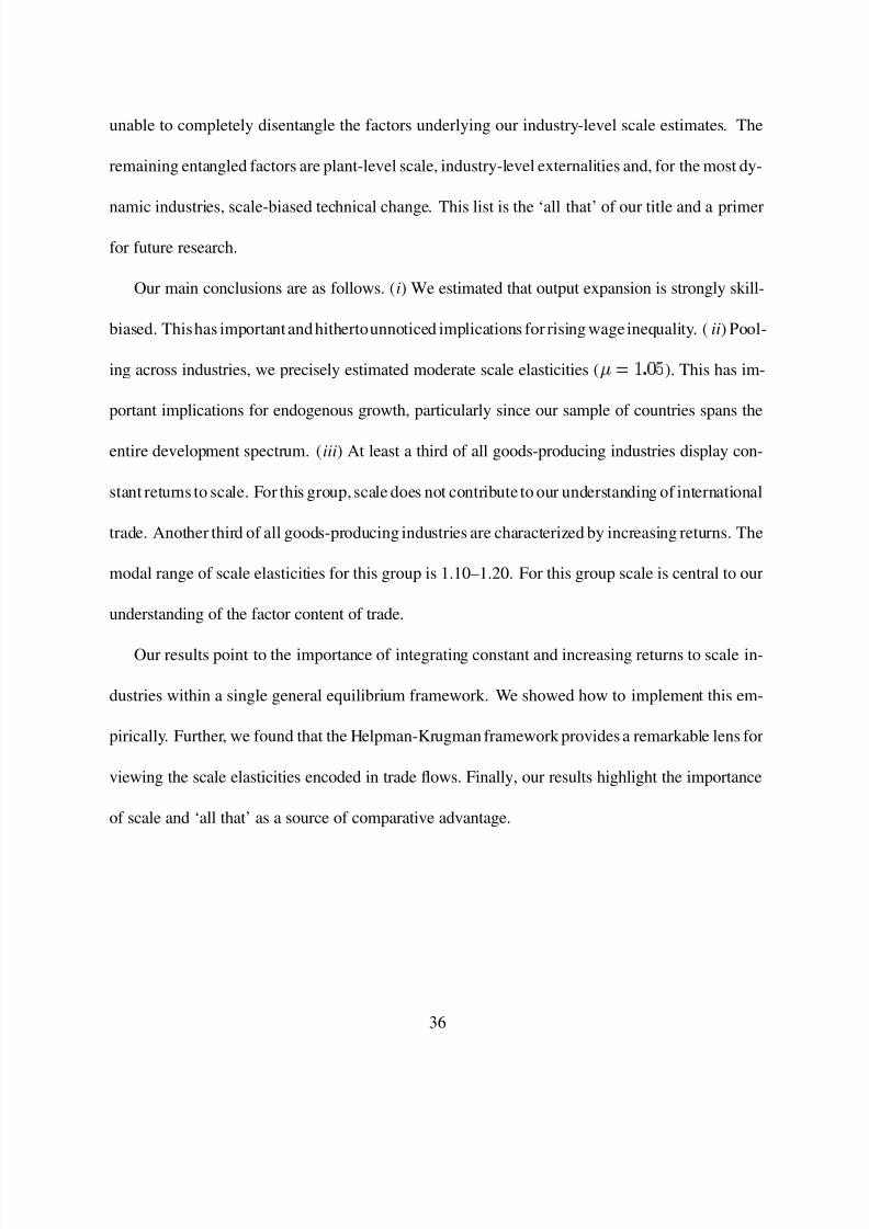
8/3/2019 Increasing Returns and All That (Antweiler and Trefler, 2002)
http://slidepdf.com/reader/full/increasing-returns-and-all-that-antweiler-and-trefler-2002 38/59
unable to completely disentangle the factors underlying our industry-level scale estimates. The
remaining entangled factors are plant-level scale, industry-level externalities and, for the most dy-
namic industries, scale-biased technical change. This list is the ‘all that’ of our title and a primer
for future research.
Our main conclusions are as follows. (i) We estimated that output expansion is strongly skill-
biased. Thishas important and hithertounnoticed implications for rising wage inequality. (ii) Pool-
ing across industries, we precisely estimated moderate scale elasticities (ç "
Q D
). This has im-
portant implications for endogenous growth, particularly since our sample of countries spans the
entire development spectrum. (iii) At least a third of all goods-producing industries display con-
stant returns to scale. For this group, scale does not contribute to our understanding of international
trade. Another third of all goods-producing industries are characterized by increasing returns. The
modal range of scale elasticities for this group is 1.10–1.20. For this group scale is central to our
understanding of the factor content of trade.
Our results point to the importance of integrating constant and increasing returns to scale in-
dustries within a single general equilibrium framework. We showed how to implement this em-
pirically. Further, we found that the Helpman-Krugman framework provides a remarkable lens for
viewing the scale elasticities encoded in trade flows. Finally, our results highlight the importance
of scale and ‘all that’ as a source of comparative advantage.
36

8/3/2019 Increasing Returns and All That (Antweiler and Trefler, 2002)
http://slidepdf.com/reader/full/increasing-returns-and-all-that-antweiler-and-trefler-2002 39/59
Appendix
A. Data and Their Sources
Data on endowments are constructed as follows. Capital stocks are from Summers and Heston
(1991). When available, we used the capital stock series. Otherwise, we used Leamer’s (1984)
double declining balance method applied to investment. Educational-attainment in the population
is from Barro and Lee (1993). We updated it to 1992. Energy is the sum of joule-equivalent re-
serves of hard coal, soft coal, crude oil, natural gas, and hydroelectric potential. Data are from the
World Resources Institute diskette and other minor sources. Land is the sum of cropland, pasture,
and forests as reported in FAO diskettes. All endowments are stocks, not flows.
For each country, industry, and year we have assembled data on international trade and produc-
tion. Table A.1 lists the countries in thedatabase. (SouthKorea was inadvertentlyomitted from our
group of 23 OECD countries.) Trade data are from the Statistics Canada “World Trade Database.”
Production data are from the UNIDO INDSTAT production data base, from the UN General Indus-
trial Statistics (including its earlier incarnations), and from other minor sources. Our 34 industries
completely cover the tradeables sector except for metal mining, non-metal mining, and miscella-
neous manufacturing. These three have no sensible production data because of aggregation prob-
lems. As a result they are included in the analysis, but are treated as constant returns to scale in-
dustries
ç
so that the estimating equations are independent of their data. We also applied the
sameç
constraint to the Crude Petroleum and Natural Gas industry for the 23-country results
in table 4. This makes little difference to the results, but seemed the sensible way to deal with trade
flows given that (i) the 23-country group omits the major oil producers and (ii) the 23-countryq
ç
for Crude Petroleum and Natural Gas is ç "
Q
. Manufacturing output was converted into 1987
U.S. dollars using IFS and PWT exchange rate data, PWT PPPs, and BEA industry-level price in-
dexes. Agricultural output was converted using FAO data. Other non-manufacturing output was
in physical units.
The U.S. choice-of-techniques matrices are fromvarious sources.ä å
¡ ¢in equation (9) is from
the benchmark input-output tables (1972, 1977, 1982, 1987, and 1992). TheÜ 5
¡ ¢in equation (8)
37
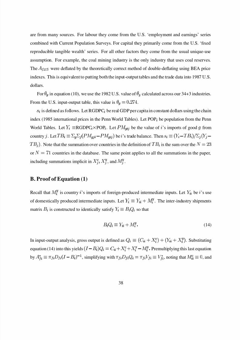
8/3/2019 Increasing Returns and All That (Antweiler and Trefler, 2002)
http://slidepdf.com/reader/full/increasing-returns-and-all-that-antweiler-and-trefler-2002 40/59
are from many sources. For labour they come from the U.S. ‘employment and earnings’ series
combined with Current Population Surveys. For capital they primarily come from the U.S. ‘fixed
reproducible tangible wealth’ series. For all other factors they come from the usual unique-use
assumption. For example, the coal mining industry is the only industry that uses coal reserves.
The 5 ¡ ¢
were deflated by the theoretically correct method of double-deflating using BEA price
indexes. This is equivalent to putting both the input-output tables and the trade data into 1987 U.S.
dollars.
Forè
in equation (10), we use the 1982 U.S. value of è
calculated across our 34+3 industries.
From the U.S. input-output table, this value isè
Q
"
Wi.
E
© is defined as follows. Let RGDPC© be real GDP per capita in constant dollars using the chain
index (1985 international prices in the Penn World Tables). Let POP© be population from the Penn
World Tables. Let n
©
9
RGDPC©
xPOP© . Let o
Y
© T be the value of ’s imports of good
from
country V . Let
ù
©
9 C
C
T
oY
T ©
P
oY
© T be ’s trade balance. Then E
©
9
n
©
P
ù
©
F C
T
n
T
P
ù
T . Note that the summation over countries in the definition of
ù
© is the sum over the%
B
or % W countries in the database. The same point applies to all the summations in the paper,
including summations implicit in f `
T
f r
T
, and Y r
T
.
B. Proof of Equation (1)
Recall thatY r
©
is country’s imports of foreign-produced intermediate inputs. Let n
© © be’s use
of domestically produced intermediate inputs. Let n
©
9
n
© ©
Yr
©
. The inter-industry shipments
matrixù
© is constructed to identically satisfy n
©
9 ù
©
© so that
ù
©
©
9
n
© ©
Y r
©
"(14)
In input-output analysis, gross output is defined as
©
9
S
© ©
f `
©
n
© ©
f r
©
. Substituting
equation (14) into this yields ø P ù
©
©
S
© ©
f `
©
f r
©P
Y r
©
"Premultiplying this last equation
by
5
© 9
7 5
©
÷
5
©
ø P ù
© Ý
, simplifying with7 5
©
÷
5
©
©
7 5
©
4 5
©
9
4
5
©
, noting thatY
`
© © 9
Q
, and
38
8/3/2019 Increasing Returns and All That (Antweiler and Trefler, 2002)
http://slidepdf.com/reader/full/increasing-returns-and-all-that-antweiler-and-trefler-2002 41/59
adding to the resultC
T i
p
©
5
T
S
© T
P C
T
5
T
Y `
© T
Q
yields
4
5
©
2
`
5
©
5
©
fr
©
P
Yr
©
C
T
5
T
S
© T (15)
where2 `
5
© 9
5
©
f `
© P C
T
5
T
Y `
© T
. Summing equation (15) across countries
and multiplying by
E
© yields
E
©
4
5 A
E
©
C
T
2
`
5
T
E
©
C
T
5
T
fr
T
P
Yr
T
E
©
C
T
5
T
S A
T . (16)
Subtracting equation (16) from equation (15) and usingC
T
2 `
5
T
Q
yields equation (1).
By the usual input-output logic, the delivery of one unit of final demand requiresG ø P ù
© Ý
units of gross output. Sinceù
© includes imported intermediates (see equation 14), the required
gross output includes foreign-produced intermediates. 5
©
9 ÷
5
©
ø P ù
© Ý
is thus the amount of
factor'
that would have been used to produce the required gross output had the required output all
been produced domestically. Since, roughly speaking,Y
r
©
of it was produced abroad, using 5
©
inflates the factor content of trade by an amount 5
©
Y r
©
. The equation(3) factorcontent expression
corrects for this by including terms likeP
5
©
Yr
©
.
C. Trade in Intermediate Inputs
In this appendix we investigate the role of our assumption about the share of trade that is trade in
intermediate inputs. LetY
`
© T 3
andY
r
© T 3
be country’s imports of good
from country
Vin year 1
for final goods and intermediate inputs, respectively. We observeY
© T 3
9
Y`
© T 3
Yr
© T 3
, but not
Y`
© T 3
orY r
© T 3
. The problem is to choose an appropriate value for the share of intermediate inputs
in total trade,
© T 3
9
Yr
© T 3
F
Y
© T 3 .
We begin by noting that the bulk of world trade is trade in intermediate inputs so that we might
conservatively expect the
© T 3 to exceed one half. Consider Canada-U.S. bilateral trade since we
are most familiar with these data. Careful examination of these data reveals that at least two thirds
of it is intermediates trade.16 This conclusion is consistent with the aggregate numbers. For the
16Government of Canada (1997) reports the averageof imports and exports for the followingcategories. Consumer
goods account for 7% of trade. None of this is intermediate inputs. Machinery and industrial goods account for 42%
39
8/3/2019 Increasing Returns and All That (Antweiler and Trefler, 2002)
http://slidepdf.com/reader/full/increasing-returns-and-all-that-antweiler-and-trefler-2002 42/59
United States in 1987, intermediate inputs plus private investment as a percentage of gross output
was 53%. The percentage is higher for the goods-producing tradeable sector i.e., for the industries
that concern us. Thus, we expect
© T 3 to exceed one half on average. We emphasize that one half
is a conservative number.
We next turn to our choice of
© T 3 . Let
¡ ¢
3 , n
¡ ¢
3 , andø
¡ ¢
3 be U.S. gross output, in-
termediate inputs, and investment in industry in year 1 . We assume that
© T 3 equals
© T 39
n
¡ ¢
3
ø
¡ ¢
3
F
¡ ¢
3 .
© T 3
ranges from 0.28 to 1.00 across our 34 industries and 5 years.
Table A.2 explores the sensitivity of our results to different choices of
© T 3 . The first row of
the table reports the ML estimateq
çfor the model with 71 countries, 11 factors, 5 years, and our
baselineassumption
© T 3
© T 3
. It is the sameq
ças in the first row of table 2. The secondrow uses
a
© T 3 that is halfway between
© T 3 and unity. The third row uses a
© T 3 that is halfway between
© T 3
and zero. It is clear that such radical changes in the choice of
© T 3 make little difference to
our estimates of scale.
The remaining rows of table A.2 set
© T 3 to a constant. It is our strong contention that
© T 3
averaged across industries should exceedone half. From table A.2, allowing
© T 3 to fall to one half
makes no difference toq
ç . Further, the loglikelihood value declines monotonically as
© T 3 moves
from unity to zero. This suggests, as expected, that the model fits the data better for large values
of
© T 3
. To conclude, our results are robust to a wide range of assumptions about the allocation of
trade between intermediate inputs and final goods.
D. GLS Variance Parameters
Theestimating equation (13) involvesa GLScorrection 7
5
© 3 . We parameterize 7
5
© 3 as 7
5
© 3
9
E
© 3
7
5
3
where E
© 3
is a control for country size and 7
5
3 is a control for factor size. is a parameter to be
of trade. All of this is intermediate inputs. Automotive goods account for 29% of trade. From the Canadian 1988input-output tables, under half of this or 12% is trade in parts. Parts are intermediate inputs. Assuming conservatively
that no finished automotive goods are intermediate inputs (e.g., treating trucks as final goods), only 12% of automotive
trade is intermediate inputs. ‘Other’ goods account for 23% of trade. ‘Other’ goods is dominated by forestry products
which in turn is primarily used as intermediates in the construction industry. We conservatively assume that only half
or 11% of ‘Other’ goods trade is intermediate inputs. The sum of 42% plus 12% plus 11% is 65%. That is, at least
two-thirds of Canada-U.S. trade is intermediates trade.
40

8/3/2019 Increasing Returns and All That (Antweiler and Trefler, 2002)
http://slidepdf.com/reader/full/increasing-returns-and-all-that-antweiler-and-trefler-2002 43/59
estimated. 7
5
3 is defined as the cross-country variance of 2
5
© 3
ç
F
E
© 3
where2
5
© 3 is defined
in equation (12). G
was chosen by an iterative procedure: pick an initial G, estimate the model
to obtain anq
, set G
equal toq
, and repeat until G
converges toq
. It quickly became clear that
theq
always lie in the tight interval
Q
" p
Q
" C B
. As a result, we set G equal to 0.9 for all the
estimates reported in the paper. (Setting G
to 0.80 or 1.00 makes no difference.) Theq
for the ML
specifications in tables 2 and 4 appear in table A.3. All of them are close to 0.90. Theq
underlying
the table 3 estimates vary between 0.85 and 0.93 across the 34 industries.
For NLS and NL2SLS, one typically replaces with a consistent estimate. We chose
Q
" C.
Allowing the variance to vary additionally across factors and years or introducing factor fixed
effects makes no difference to the estimates. For one, the effect of scaling by 7
5
3 is that factors
have similar variances in each year. For another,2
5
© 3
ç
has a zero mean for each factor.
E. Details of the NL2SLS Estimators
Let 1 " " " 1 G be the years lost as a result of instrumenting using lagged regressors. We are
interested in ‘within’ estimators. Let 5
© 3 be any variable and let be an operator that transforms
5
© 3 by subtracting off its mean across all factors' " " " 2
and years 1 1 G
" " " . That is,
5
© 3
9
5
© 3
P C
5 z
C
3
z{
3
5 z
© 3
z
F
2
P
1G
.
The NL2SLS estimator is based on Amemiya (1974). Consider the ‘ Q 2
5
©
3
Ý R
ç
’ esti-
mator. From equation (13), let
@
ç
be the2 %
P
1G
x vector formed by stacking the
@
5
© 3
ç
2
5
© 3
ç
F
7
5
© 3 . Let Q
e
5
© 3
ç
9|
2
5
©
3
Ý
3
ç
F
7
5
© 3 } } }
2
5
©
3
Ý
3
ç
F
7
5
© 3
e
be the x f
vector of instruments. Let Q
e
ç
be the corresponding2 %
P
1G
x fmatrix
of stacked instruments. The ‘ Q 2
5
©
3
Ý R
ç
’ estimator minimizes
@
ç
o
e
ç
@
ç
where
o
e
ç
9
Q
e
Q
e
Q
e Ý
Q
e . Let ç
e
G
be the minimizer. Since Q
e
ç
is a function of ç , the in-
struments must be simultaneously estimated along with the rest of the model. That is, NL2SLS is
a 1-stage estimator, not a 2-stage one.
Consider the ‘¥
q
2
5
© 3 F
¥
ç’ estimator. Let be the dimension of
ç, define the gradient
w 5
© 3
ç
9
¥
2
5
© 3 F
¥
ç
F
7
5
© 3 , and letw
ç
be the2 %
P
1G
x matrix of stacked
w 5
© 3
ç
. In the first
stage, instrumentw
ç
e
G
by Q
e
ç
e
G
to obtainq
w
9
o
e
ç
e
G
w
ç
e
G
. In thesecond stage,minimize
41
8/3/2019 Increasing Returns and All That (Antweiler and Trefler, 2002)
http://slidepdf.com/reader/full/increasing-returns-and-all-that-antweiler-and-trefler-2002 44/59
@
ç
o
ç
e
G
@
ç
where o
ç
e
G
9
q
w
q
w
q
w
Ý
q
w
. Denote the minimizer byç
e
. In table 2,
ç
e
dependson f only viaç
e
G
. Also, the table2 conclusions are robust to expandingtheinstrument
setq
wto include polynomials and cross-products of
q
w.17
1 -statistics for the two NL2SLS estimators are based on the covariance matricesq
7
§
w
ç
e
G
o
e
ç
e
G
w
ç
e
G
Ý
andq
7
§
w
ç
e
o
ç
e
G
w
ç
e
Ý
whereq
7 is the model standard error (based
on unprojectedresiduals, of course). The Hausman test is basedon the difference between theNLS
and NL2SLS estimates.
17In table 2, the standard errors of the two NL2SLS estimators are similar and occasionally the ‘×
q
¤
Ù
×
ñ’ stan-
dard errors are (unexpectedly) larger. When squares and cross-products of q
are included in the instrument set, the
‘×
q
¤
Ù
×
ñ’ standard errors are always lower, but not significantly so.
42
8/3/2019 Increasing Returns and All That (Antweiler and Trefler, 2002)
http://slidepdf.com/reader/full/increasing-returns-and-all-that-antweiler-and-trefler-2002 45/59
References
Amemiya, Takeshi (1974) “The Nonlinear Two-Stage Least-Squares Estimator,” Journal of
Econometrics, 2 (2), 105–110.
(1975) “The Nonlinear Limited-Information Maximum-Likelihood Estimator and the Mod-ified Nonlinear Two-Stage Least-Squares Estimator,” Journal of Econometrics, 3 (4), 375–
386.
Antweiler, Werner and Daniel Trefler (1997) “Increasing Returns and All That: A View From
Trade.” Mimeo, University of Toronto.
Baily, Martin Neil and Hans Gersbach (1995) “Efficiency in Manufacturing and the Need for
Global Competition,” Brookings Papers on Economic Activity, Microeconomics, 307–358.
Barro, Robert and Jong-Wha Lee (1993) “International Comparisons of Educational Attain-
ment,” Journal of Monetary Economics, 32 (3), 363–394.
Basu, Susanto (1995) “Procyclical Productivity: Increasing Returns or Cyclical Utilization?,”
Quarterly Journal of Economics, 111 (3), 719–751.
and John G. Fernald (1997) “Returns to Scale in U.S. Production: Estimates and Implica-
tions,” Journal of Political Economy, 105 (2), 249–279.
Bowen, Harry P., Edward E. Leamer, and Leo Sveikauskas (1987) “Multicountry, Multifactor
Tests of the Factor Abundance Theory,” American Economic Review, 77 (5), 791–809.
Brainard, S. Lael (1993) “An Empirical Assessment of the Factor Proportions Explanation of
Multinational Sales.” NBER Working Paper #4580.
(1997) “An Empirical Assessment of the Proximity/Concentration Tradeoff between Multi-
national Sales and Trade,” American Economic Review, 87 (4), 520–540.
Conway, Patrick J. (2000) “The Case of the Missing Trade and other Mysteries: Comment.”
Mimeo, University of North Carolina.
Davis, Donald R. (1995) “Intra-industry Trade: A Heckscher-Ohlin-Ricardo Approach,” Journal
of International Economics, 39 (3-4), 201–226.
(1997) “Critical Evidence on Comparative Advantage? North-North Trade in a Multilateral
World,” Journal of Political Economy, 105 (5), 1051–1060.
and David E. Weinstein (1996) “Does Economic Geography Matter for International Spe-
cialization?” NBER Working Paper #5706.
and (1998) “An Account of the Global Factor Content of Trade.” NBER WorkingPaper
#6785.
43
8/3/2019 Increasing Returns and All That (Antweiler and Trefler, 2002)
http://slidepdf.com/reader/full/increasing-returns-and-all-that-antweiler-and-trefler-2002 46/59
Deardorff, Alan V. (1979) “Weak Links in the Chain of Comparative Advantage,” Journal of In-
ternational Economics, 9 (2), 197–209.
Denny, Michael and Melvyn Fuss (1983) “TheEffectsof Factor Prices andTechnologicalChange
on the Occupational Demand for Labor: Evidence from Canadian Telecommunications,”
Journal of Human Resources, 18 (2), 161–176.
Epstein, Larry G. (1982) “Integrability of Incomplete Systems of Demand Functions,” Review of
Economic Studies, 49 (3), 411–425.
Ethier, Wilfred J. (1982) “National and International Returns to Scale in the Modern Theory of
International Trade,” American Economic Review, 72 (3), 389–405.
Feenstra, Robert C. and Gordon H. Hanson (1996a) “Foreign Investment, Outsourcing, and
Relative Wages,” in Robert C. Feenstra, Gene M. Grossman, and Douglas A. Irwin, eds., The
Political Economy of Trade Policy: Papers in Honor of Jagdish Bhagwati , Cambridge MA:
MIT Press.
and (1996b) “Globalization, Outsourcing, and Wage Inequality,” American Economic
Review Papers and Proceedings, 86 (2), 240–245.
and (1997) “Foreign Direct Investment and Relative Wages: Evidence from Mexico’s
Maquiladoras,” Journal of International Economics, 42 (3-4), 371–193.
Food and Agricultural Organization of the United Nations (1992) “Intercountry Comparisons
of Agricultural Output and Productivity: Revised Methodology and Empirical Results,” FAO
Quarterly Bulletin of Statistics, 5 (4), iii–vi.
Fuss, Melvyn A. and V. K. Gupta (1981) “A Cost Function Approach to the Estimation of Min-imum Efficient Scale, Returns to Scale, and Suboptimal Capacity,” European Economic Re-
view, 15 (2), 123–135.
Government of Canada (1997) “NAFTA: A Partnership at Work.” Department of Foreign Affairs
and International Trade, http://www.dfait-maeci.gc.ca/nafta-alena/what2-e.asp.
Griliches, Zvi and Jacques Mairesse (1995) “Production Functions: The Search for Identifica-
tion.” NBER Working Paper #5067.
and Vidar Ringstad (1971) Economies of Scale and the Form of the Production Function:
An Econometric Study of Norwegian Manufacturing Establishment Data, Amsterdam: North
Holland.
Harrigan, James (1993) “OECD Imports and Trade Barriers in 1983,” Journal of International
Economics, 35 (1-2), 91–111.
(1996) “Openness to Trade in Manufactures in the OECD,” Journal of International Eco-
nomics, 40 (1-2), 23–39.
44

8/3/2019 Increasing Returns and All That (Antweiler and Trefler, 2002)
http://slidepdf.com/reader/full/increasing-returns-and-all-that-antweiler-and-trefler-2002 47/59
(1999) “Estimationof Cross-Country Differences in IndustryProduction Functions,” Journal
of International Economics, 47 (2), 267–93.
Helpman, Elhanan (1981) “International Trade in the Presence of Product Differentiation,
Economies of Scale and Monopolistic Competition: A Chamberlin-Heckscher-Ohlin Ap-
proach,” Journal of International Economics, 11 (3), 305–340.
(1987) “Imperfect Competition and International Trade: Evidence from Fourteen Industrial
Countries,” Journal of the Japanese and International Economies, 1 (1), 62–81.
and Paul R. Krugman (1985) Market Structure and Foreign Trade, Cambridge, MA: MIT
Press.
Hummels, David and James Levinsohn (1993) “Product Differentiation as a Source of Compar-
ative Advantage?,” American Economic Review Papers and Proceedings, 83 (2), 445–449.
and (1995) “International Trade and Monopolistic Competition: Reconsidering the Ev-
idence,” Quarterly Journal of Economics, 110 (3), 799–836.
Jorgenson, Dale W. and Jean-Jacques Laffont (1974) “Efficient Estimation of Nonlinear Simul-
taneous Equations with Additive Disturbances,” Annals of Economic and Social Measure-
ment , 3 (4), 615–640.
Klepper, Steven and Edward E. Leamer (1984) “Consistent Sets of Estimates for Regressions
with Errors in All Variables,” Econometrica, 52 (1), 163–183.
Krugman, Paul R. (1979) “Increasing Returns, Monopolistic Competition, and International
Trade,” Journal of International Economics, 9 (4), 469–479.
(1991) Geography and Trade, Cambridge, MA: MIT Press.
Lancaster, Kelvin (1984) “Protection and Product Differentiation,” in Henryk Kierzkowski, ed.,
Monopolistic Competition and International Trade, Oxford: Oxford University Press.
Leamer, Edward E. (1984) Sources of International Comparative Advantage: Theory and Evi-
dence, Cambridge, MA: MIT Press.
Levinsohn, James and Amil Petrin (1999) “When Industries Become More Productive, Do
Firms? Investigating Productivity Dynamics.” Mimeo, University of Michigan.
Markusen, James R. and Anthony J. Venables (1998) “Multinational Firms and the New Trade
Theory,” Journal of International Economics, 46 (2), 183–203.
Nelson, Charles R. and Richard Startz (1990)“Some Further Results on theExactSmallSample
Properties of the Instrumental Variables Estimator,” Econometrica, 58 (4), 967–976.
Olley, G. Steven and Ariel Pakes (1996) “The Dynamics of Productivity in the Telecommunica-
tions Equipment Industry,” Econometrica, 64 (6), 1263–1297.
45
8/3/2019 Increasing Returns and All That (Antweiler and Trefler, 2002)
http://slidepdf.com/reader/full/increasing-returns-and-all-that-antweiler-and-trefler-2002 48/59
Paul, Catherine J. Morrison and Donald S. Siegel (1999) “Scale Economies and Industry Ag-
glomeration Externalities: A Dynamic Cost Function Approach,” American Economic Re-
view, 89 (2), 272–290.
Rosenberg, Nathan (1982) Inside the Black Box: Technology and Economics, Cambridge: Cam-
bridge University Press.
(1994) Exploring the Black Box: Technology, Economics, and History, Cambridge: Cam-
bridge University Press.
Rotemberg, Julio and Michael Woodford (1992) “Oligopolistic Pricing and the Effects of Ag-
gregate Demand on Economic Activity,” Journal of Political Economy, 100 (6), 1153–1207.
Summers, Robert and Alan Heston (1991) “The Penn World Table (Mark 5): An Expanded Set
of International Comparisons, 1950-1988,” Quarterly Journal of Economics, 106 (2),327–68.
Trefler, Daniel (1993) “International Factor Price Differences: Leontief was Right!,” Journal of
Political Economy, 101 (6), 961–987.
(1995) “The Case of the Missing Trade and Other Mysteries,” American Economic Review,
85 (5), 1029–1046.
(1996) “The Structure of Factor Content Predictions.” Mimeo, University of Chicago.
Tybout, James R. (2000) “Manufacturing Firms in Developing Countries: How Well Do They
Do, and Why?,” Journal of Economic Literature, 38 (1), 11–44.
and M. Daniel Westbrook (1995) “Trade Liberalization and the Dimensions of Efficiency
Change in Mexican Manufacturing Industries,” Journal of International Economics, 39 (1-2),53–78.
Vanek, Jaroslav (1968) “The Factor Proportions Theory: The N-Factor Case,” Kyklos, 21, 749–
56.
46
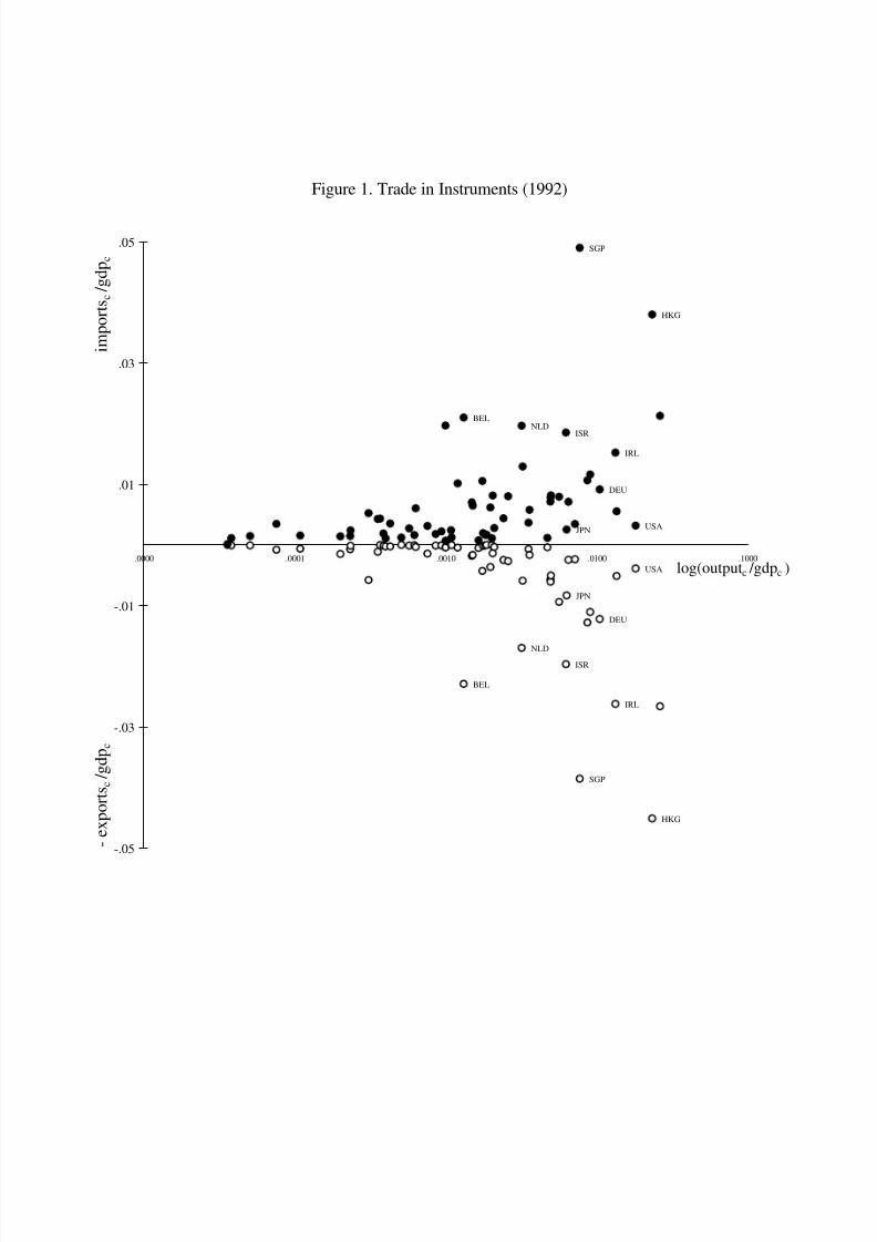
8/3/2019 Increasing Returns and All That (Antweiler and Trefler, 2002)
http://slidepdf.com/reader/full/increasing-returns-and-all-that-antweiler-and-trefler-2002 49/59
Figure 1. Trade in Instruments (1992)
BEL
NLDISR
JPN
SGP
DEU
IRL
USA
HKG
BELNLD
ISR
JPN
SGP
DEU
IRL
USA
HKG
-.05
-.03
-.01
.01
.03
.05
.0000 .0001 .0010 .0100 .1000
- e x p o r t s c / g d p c
i m p o r t s c / g d p c
log(outputc /gdpc )

8/3/2019 Increasing Returns and All That (Antweiler and Trefler, 2002)
http://slidepdf.com/reader/full/increasing-returns-and-all-that-antweiler-and-trefler-2002 50/59
Figure 2. U.S. Bilateral Trade in Instruments (1992)
HKGIRL
DEUSWE
SGP
JPN
IRL
DEU
SGP
JPN
HKG
.00001 .00011 .00101 .01001 .10001
l o g
( i m p o r t s U S / g d p c )
l o g ( e x p o r t s U S / g d p c )
log(outputc /gdpc )
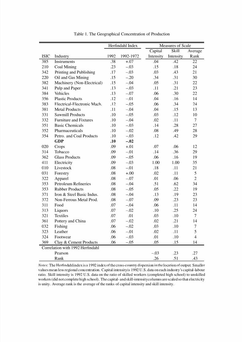
8/3/2019 Increasing Returns and All That (Antweiler and Trefler, 2002)
http://slidepdf.com/reader/full/increasing-returns-and-all-that-antweiler-and-trefler-2002 51/59
Table 1. The Geographical Concentration of Production
Herfindahl Index Measures of Scale
Capital Skill Average
ISIC Industry 1992 1992-1972 Intensity Intensity Rank
385 Instruments .38 +.07 .04 .42 22
210 Coal Mining .23 –.03 .15 .18 24
342 Printing and Publishing .17 –.03 .03 .43 21
220 Oil and Gas Mining .15 –.20 .34 .31 30
382 Machinery (Non-Electrical) .15 –.04 .05 .31 22
341 Pulp and Paper .13 –.03 .11 .21 23
384 Vehicles .13 –.07 .06 .30 22
356 Plastic Products .12 –.01 .04 .16 14
383 Electrical-Electronic Mach. .12 –.05 .06 .34 24
381 Metal Products .11 –.04 .04 .15 13
331 Sawmill Products .10 –.05 .03 .12 10
332 Furniture and Fixtures .10 –.04 .02 .11 7351 Basic Chemicals .10 –.03 .14 .28 27
352 Pharmaceuticals .10 –.02 .08 .49 28
354 Petro. and Coal Products .10 –.03 .12 .42 29
GDP .10 –.02
020 Crops .09 +.01 .07 .06 12
314 Tobacco .09 –.01 .14 .36 29
362 Glass Products .09 –.05 .06 .16 19
411 Electricity .09 –.03 1.00 1.00 35
010 Livestock .08 –.01 .18 .11 21
031 Forestry .08 +.00 .02 .11 5
322 Apparel .08 –.07 .01 .06 2353 Petroleum Refineries .08 –.04 .51 .62 34
353 Rubber Products .08 –.05 .05 .22 19
371 Iron & Steel Basic Indus. .08 –.04 .13 .19 23
372 Non-Ferrous Metal Prod. .08 –.07 .09 .23 23
311 Food .07 –.04 .06 .11 14
313 Liquors .07 –.02 .10 .25 24
321 Textiles .07 –.01 .03 .10 7
361 Pottery and China .07 –.02 .02 .21 14
032 Fishing .06 –.02 .03 .10 7
323 Leather .06 –.01 .02 .11 5
324 Footwear .06 –.03 .01 .10 4
369 Clay & Cement Products .06 –.05 .05 .15 14
Correlation with 1992 Herfindahl
Pearson –.03 .23 .27
Rank .26 .51 .43
Notes: The Herfindahlindexis a 1992 indexof thecross-country dispersion in the locationof output. Smaller
values mean less regional concentration. Capital intensityis 1992 U.S.data on each industry’s capital-labour
ratio. Skill intensity is 1992 U.S. data on the ratio of skilled workers (completed high school) to unskilled
workers (did not complete high school). The capital- andskill-intensitycolumns are scaledso that electricity
is unity. Average rank is the average of the ranks of capital intensity and skill intensity.

8/3/2019 Increasing Returns and All That (Antweiler and Trefler, 2002)
http://slidepdf.com/reader/full/increasing-returns-and-all-that-antweiler-and-trefler-2002 52/59
T a b l e 2 . T h e E l a s t i c i t y o f S c a l e f o r D i f f e r e n t E s t i m a t o r s : P o o l i n g A c r o s s I n d u s t r i e s
M L
N L S
N L 2 S
L S
N L 2 S L S
R o w
Y e a r s
t
t
L a g L e n g t h
K
t
t
( 1 )
1 9 7 2 - 9 2
1 . 0 5 1
1 3 . 4 1
1 . 0 5 0
1 2 . 5 6
( 2 )
1 9 8 7 - 9 2
1 . 0 4 5
6 . 7 5
1 . 0 4 4
6 . 1 1
1 5 Y e a r s
1
1 . 0 9 5
1 4 . 0 3
1 . 0 9 5
1 4 . 0 3
( 3 )
3
1 . 0 9 8
1 5 . 0 5
1 . 0 9 5
1 4 . 1 3
( 4 )
5
1 . 0 9 8
1 5 . 2 3
1 . 0 9 5
1 4 . 2 4
( 5 )
1 9 8 2 - 9 2
1 . 0 4 8
9 . 4 7
1 . 0 4 7
8 . 6 7
1 0 Y e a r s
1
1 . 0 8 8
1 6 . 6 7
1 . 0 8 8
1 6 . 6 7
( 6 )
3
1 . 0 9 1
1 7 . 9 1
1 . 0 8 8
1 6 . 8 9
( 7 )
5
1 . 0 9 0
1 7 . 8 2
1 . 0 8 8
1 7 . 0 5
( 8 )
1 9 9 2
1 . 0 3 7
3 . 5 8
1 . 0 3 7
3 . 2 1
2 0 Y e a r s
1
1 . 0 9 8
9 . 0 0
1 . 0 9 8
9 . 0 0
( 9 )
3
1 . 0 9 8
9 . 6 5
1 . 0 9 8
9 . 6 6
( 1 0 )
5
1 . 0 6 5
4 . 8 0
1 . 0 8 4
7 . 5 9
N o t e s : a . T
h i s t a b l e r e p o r t s e s t i m a t e s o f t h e e l a s t i c i t y o f s c a l e
f o r t h e c a s e w h e r e a l l i n d u s t r i e s a r e a s s u m e d t o s h a r e a c o m m
o n
.
t i s t h e t - s t a t i s t i c f o r t h e h y p o t h e s i s o f c o n s t a n t r e t u r n s t o s c a l e (
= 1 ) .
b . E a c h e s t i m a t e u s e s a l l 7 1 c o u n t r i e s a n d a l l 1 1 f a c t o r s . T h e 1 1 f a c t o r s a r e c a p i t a l , 4 t y
p e s o f l a b o u r ( n o e d u c a t i o n , p r i m a r y e
d u c a -
t i o n , s e c o n d a r y e d u c a t i o n , a n d p o s t - s e c o n d a r y e d u c a t i o n ) , 3 t y p e s o f l a n d ( c r o p l a n d , p a s
t u r e , a n d f o r e s t ) , a n d 3 t y p e s o f e n e r g y
( c o a l
r e s e r v e s , o i l a n d g a s r e s e r v e s , a n d h y d r o e l e c t r i c p o t e n t i a l ) . T h e n u m b e r o f y e a r s
u s e d v a r i e s a c r o s s s p e c i fi c a t i o n s . W e u s e
e v e r y
fi f t h y e a r o f d a t a o v e r t h e p e r i o d i n d i c a t e d i n t h e ‘ Y e a r s ’ c o l u m n . T h e n u m b e r o f o b s e r v
a t i o n s i s
.
c . T h e N L 2 S L S c o l u m n s r e p o r t t h e i n s t r u m e n t a l
v a r i a b l e s r e s u l t s . T h e
ª
¬
-
®
i n s t r u m e n t s e t u s e s l a g s o f o r d e r
g i v e n
b y t h e ‘ L a g L e n g t h ’ c o l u m n . T h e i n s t r u m e n t s e t
a l s o i n c l u d e s p o l y n o m i a l s o f t h e
ª
¬
-
®
w h e r e t h e p o l y n o m i a l o r d e r i s
g i v e n
b y t h e ‘ K ’ c o l u m n . T h e m o r e c o m p l i c a t e d
°
±
°
i n s t r u m e n t s e t c o n s i s t s o f fi t t e d v a l u e s o f t h e
°
±
°
o b t a i n e d f r o m a
p r e l i m i n a r y N L 2 S L S p r o c e d u r e . S e e a p p e n d i x E
f o r d e t a i l s .
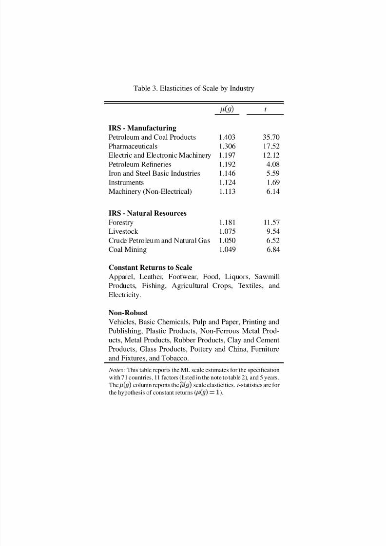
8/3/2019 Increasing Returns and All That (Antweiler and Trefler, 2002)
http://slidepdf.com/reader/full/increasing-returns-and-all-that-antweiler-and-trefler-2002 53/59
Table 3. Elasticities of Scale by Industry
²³ µ · t
IRS - Manufacturing
Petroleum and Coal Products 1.403 35.70
Pharmaceuticals 1.306 17.52
Electric and Electronic Machinery 1.197 12.12
Petroleum Refineries 1.192 4.08
Iron and Steel Basic Industries 1.146 5.59
Instruments 1.124 1.69
Machinery (Non-Electrical) 1.113 6.14
IRS - Natural Resources
Forestry 1.181 11.57
Livestock 1.075 9.54
Crude Petroleum and Natural Gas 1.050 6.52
Coal Mining 1.049 6.84
Constant Returns to Scale
Apparel, Leather, Footwear, Food, Liquors, Sawmill
Products, Fishing, Agricultural Crops, Textiles, andElectricity.
Non-Robust
Vehicles, Basic Chemicals, Pulp and Paper, Printing and
Publishing, Plastic Products, Non-Ferrous Metal Prod-
ucts, Metal Products, Rubber Products, Clay and Cement
Products, Glass Products, Pottery and China, Furniture
and Fixtures, and Tobacco.
Notes: This table reports the ML scale estimates for the specification
with 71 countries, 11 factors (listed in the note to table 2), and 5 years.
The ¹º ¼ ¾ column reports the ¿¹
º ¼ ¾ scale elasticities. t -statistics are for
the hypothesis of constant returns ( ¹º ¼ ¾ À Á ).
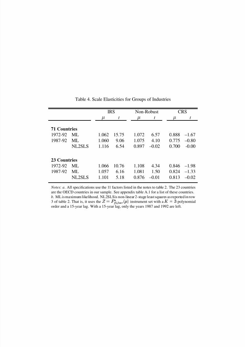
8/3/2019 Increasing Returns and All That (Antweiler and Trefler, 2002)
http://slidepdf.com/reader/full/increasing-returns-and-all-that-antweiler-and-trefler-2002 54/59
Table 4. Scale Elasticities for Groups of Industries
IRS Non-Robust CRS²
t ²
t ²
t
71 Countries
1972-92 ML 1.062 15.75 1.072 6.57 0.888 –1.67
1987-92 ML 1.060 9.06 1.075 4.10 0.775 –0.80
NL2SLS 1.116 6.54 0.897 –0.02 0.700 -0.00
23 Countries
1972-92 ML 1.066 10.76 1.108 4.34 0.846 –1.98
1987-92 ML 1.057 6.16 1.081 1.50 0.824 –1.33
NL2SLS 1.101 5.18 0.876 –0.01 0.813 –0.02
Notes: a. All specifications use the 11 factors listed in the notes to table 2. The 23 countries
are the OECD countries in our sample. See appendix table A.1 for a list of these countries.
b. MLis maximum likelihood. NL2SLSis non-linear 2-stage least squares as reported in row
3 of table 2. That is, it uses the ÃÀ Å Æ
È
É Ê Ë Í
º¹ ¾
instrument set with a ÏÀ Ñ
polynomial
order and a 15-year lag. With a 15-year lag, only the years 1987 and 1992 are left.

8/3/2019 Increasing Returns and All That (Antweiler and Trefler, 2002)
http://slidepdf.com/reader/full/increasing-returns-and-all-that-antweiler-and-trefler-2002 55/59
Table 5. Sensitivity Analysis: ²³ µ · for Different Specifications
Countries Ó =71 Ó =71 Ó =23 Ó =71
Factors Ô =11 Ô =11 Ô =11 Ô =7
Initial Rank Baseline Alternative Baseline BaselineIRS - Manufacturing
Petroleum and Coal Products 1.40ÕÕ Õ
1.40 ÕÕ Õ
1.38 ÕÕ Õ
1.38 ÕÕ Õ
Pharmaceuticals 1.31 ÕÕ Õ 1.30 Õ
Õ Õ 1.33 ÕÕ Õ 1.28 Õ
Õ Õ
Electric and Electronic Machinery 1.20Õ
Õ Õ
1.20Õ
Õ Õ
1.18Õ
1.19Õ
Õ Õ
Petroleum Refineries 1.19Õ
1.19Õ
1.20 1.20Õ
Iron and Steel Basic Industries 1.15ÕÕ
1.08 1.00 1.14 Õ
Instruments 1.12 1.15Õ
1.24Õ
Õ
1.22Õ
Õ Õ
Machinery (Non-Electrical) 1.11Õ
Õ
1.10Õ
1.15Õ
Õ
1.12Õ
Õ
IRS - Natural Resources
Forestry 1.18 ÕÕ Õ
1.18 ÕÕ Õ
1.05 Õ 1.18 ÕÕ Õ
Livestock 1.08 ÕÕ
1.08 ÕÕ
1.15 ÕÕ Õ
1.02
Crude Petroleum & Natural Gas 1.05 ÕÕ
1.05 ÕÕ
1.01 1.06 ÕÕ
Coal Mining 1.05 ÕÕ 1.05 Õ
Õ 1.05 ÕÕ 0.97
Non-Robust
Vehicles 1.02 1.02 1.09 0.97
Basic Chemicals 1.06 1.06 1.20 Ö 1.02
Pulp and Paper 1.15 1.12 1.19 Ö
Printing and Publishing 1.00 1.01
Plastic Products 1.11 1.08 1.28 Ö 1.06
Non-Ferrous Metal Products 1.24 Ö
Metal Products 1.02 1.00 1.02
Rubber Products 1.23 Ö 0.99 Ö 1.13 1.24 Ö
Clay and Cement Products 1.07 1.03 1.03
Glass Products 1.02 1.02 1.00 1.02
Pottery and China 0.83 0.83 1.01
Furniture and Fixtures 0.76
Tobacco 1.08
Notes: a. This table reports the ML scale estimates ¿¹º ¼ ¾
. There are 71 countries in the sample, 23 of which are
OECD members. The 11 factors are listed in the note to table 2. The 7 factors aggregate the 3 land factors and
aggregate the 3 energy factors. All 5 years of data are used.
b. The ‘Baseline’ initial rank columns initiate theestimation algorithmwith a ranking based on industries’ capital
and skill intensities. The ‘Alternative’ initial rank column initiates the algorithm with a ranking based on scale
elasticities from Paul and Siegel (1999).
c. A Æ indicates significance at the 1% level ( ×Ø Ù Ú Û Ü
). ÆÆ
and ÆÆ Æ
indicate ×Ø Û
and ×Ø Á á
, respectively.
d . For the IRS groups, the data are from the 10th iteration. For the Non-Robust group, the data are averages of
the 9th and 10th iterations. No t -statistics are reported for the Non-Robust group.
e. For the Non-Robust group an empty cell denotes constant returns (insignificant ¹º ¼ ¾
) in both iterations. A â
denotes increasing returns (significant ¹º ¼ ¾
) in both iterations.
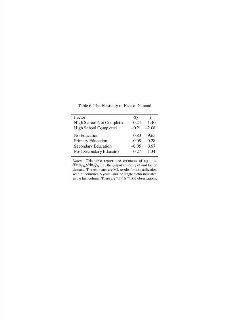
8/3/2019 Increasing Returns and All That (Antweiler and Trefler, 2002)
http://slidepdf.com/reader/full/increasing-returns-and-all-that-antweiler-and-trefler-2002 56/59
Table 6. The Elasticity of Factor Demand
Factor ãä
t
High School Not Completed 0.21 1.40
High School Completed –0.21 –2.08
No Education 0.83 9.65
Primary Education –0.08 –0.28
Secondary Education –0.05 –0.67
Post-Secondary Education –0.27 –1.34
Notes: This table reports the estimates of æ
È
À
çè é ê
Èì
í
çè é î
ì
i.e., the output elasticity of unit factor
demand. The estimates are ML results for a specificationwith 71 countries, 5 years, and the single factor indicated
in the first column. There are ïÁ ð Û À Ñ Û Û observations.
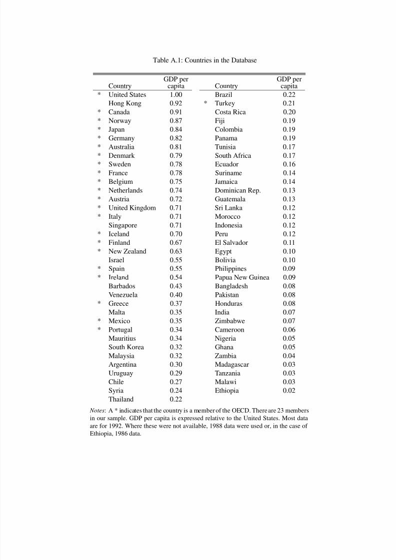
8/3/2019 Increasing Returns and All That (Antweiler and Trefler, 2002)
http://slidepdf.com/reader/full/increasing-returns-and-all-that-antweiler-and-trefler-2002 57/59
Table A.1: Countries in the Database
GDP per GDP perCountry capita Country capita
* United States 1.00 Brazil 0.22Hong Kong 0.92 * Turkey 0.21
* Canada 0.91 Costa Rica 0.20
* Norway 0.87 Fiji 0.19
* Japan 0.84 Colombia 0.19
* Germany 0.82 Panama 0.19
* Australia 0.81 Tunisia 0.17
* Denmark 0.79 South Africa 0.17
* Sweden 0.78 Ecuador 0.16
* France 0.78 Suriname 0.14
* Belgium 0.75 Jamaica 0.14
* Netherlands 0.74 Dominican Rep. 0.13
* Austria 0.72 Guatemala 0.13
* United Kingdom 0.71 Sri Lanka 0.12
* Italy 0.71 Morocco 0.12
Singapore 0.71 Indonesia 0.12
* Iceland 0.70 Peru 0.12
* Finland 0.67 El Salvador 0.11
* New Zealand 0.63 Egypt 0.10
Israel 0.55 Bolivia 0.10
* Spain 0.55 Philippines 0.09
* Ireland 0.54 Papua New Guinea 0.09
Barbados 0.43 Bangladesh 0.08
Venezuela 0.40 Pakistan 0.08* Greece 0.37 Honduras 0.08
Malta 0.35 India 0.07
* Mexico 0.35 Zimbabwe 0.07
* Portugal 0.34 Cameroon 0.06
Mauritius 0.34 Nigeria 0.05
South Korea 0.32 Ghana 0.05
Malaysia 0.32 Zambia 0.04
Argentina 0.30 Madagascar 0.03
Uruguay 0.29 Tanzania 0.03
Chile 0.27 Malawi 0.03
Syria 0.24 Ethiopia 0.02Thailand 0.22
Notes: A * indicates that the country is a member of the OECD. Thereare 23 members
in our sample. GDP per capita is expressed relative to the United States. Most data
are for 1992. Where these were not available, 1988 data were used or, in the case of
Ethiopia, 1986 data.
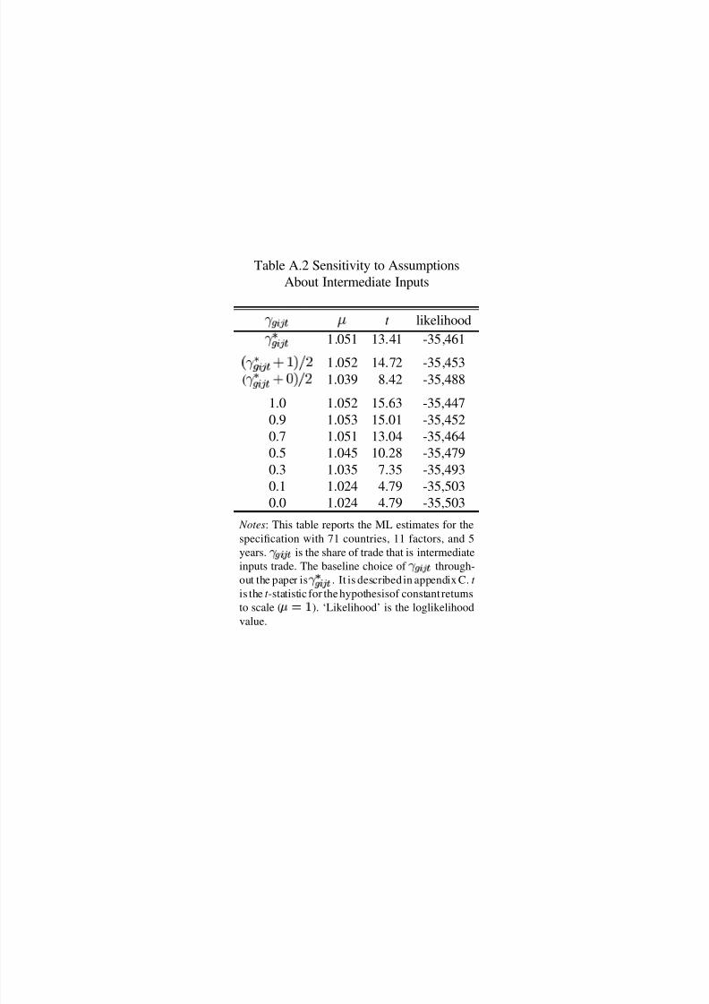
8/3/2019 Increasing Returns and All That (Antweiler and Trefler, 2002)
http://slidepdf.com/reader/full/increasing-returns-and-all-that-antweiler-and-trefler-2002 58/59
Table A.2 Sensitivity to Assumptions
About Intermediate Inputs
òó ô õ ö ² t likelihood
ò
Õ
óô õ ö 1.051 13.41 -35,461
³ò
Õ
óô õ ö ÷ ø
·ú û 1.052 14.72 -35,453
( ò
Õ
óô õ ö ÷ ü
·ú û 1.039 8.42 -35,488
1.0 1.052 15.63 -35,447
0.9 1.053 15.01 -35,452
0.7 1.051 13.04 -35,464
0.5 1.045 10.28 -35,479
0.3 1.035 7.35 -35,493
0.1 1.024 4.79 -35,503
0.0 1.024 4.79 -35,503
Notes: This table reports the ML estimates for thespecification with 71 countries, 11 factors, and 5
years. ý
ì
þ Êis the share of trade that is intermediate
inputs trade. The baseline choice of ý
ì
þ Êthrough-
out the paper is ýÆ
ì
þ Ê
. It is describedin appendix C. t
is the t -statistic for thehypothesisof constant returns
to scale ( ¹À Á
). ‘Likelihood’ is the loglikelihood
value.
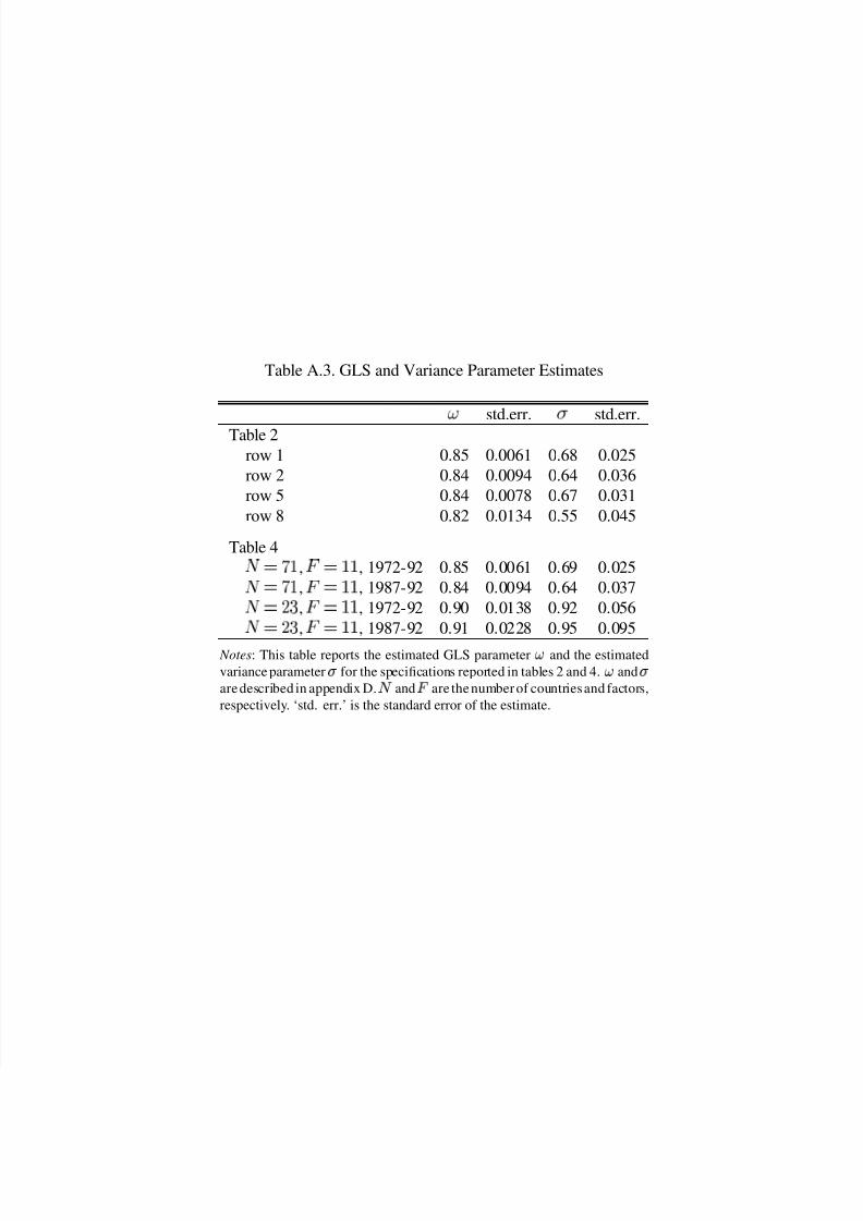
8/3/2019 Increasing Returns and All That (Antweiler and Trefler, 2002)
http://slidepdf.com/reader/full/increasing-returns-and-all-that-antweiler-and-trefler-2002 59/59
Table A.3. GLS and Variance Parameter Estimates
¡ std.err. ¢ std.err.
Table 2
row 1 0.85 0.0061 0.68 0.025
row 2 0.84 0.0094 0.64 0.036
row 5 0.84 0.0078 0.67 0.031
row 8 0.82 0.0134 0.55 0.045
Table 4
Ó£
¥
ø , Ô£
øø , 1972-92 0.85 0.0061 0.69 0.025
Ó£
¥
ø , Ô£
øø , 1987-92 0.84 0.0094 0.64 0.037
Ó£
û§ , Ô
£
øø , 1972-92 0.90 0.0138 0.92 0.056
Ó£
û§ , Ô
£
øø , 1987-92 0.91 0.0228 0.95 0.095
Notes: This table reports the estimated GLS parameter©
and the estimated
variance parameter
for the specifications reported in tables 2 and 4.©
and
aredescribed in appendix D.
and Å are thenumber of countriesand factors,
respectively. ‘std. err.’ is the standard error of the estimate.