Noname manuscript No.(will be inserted by the editor)

Incremental Development of Software Quality PredictionModels

First Author · Second Author

Received: date / Accepted: date

Abstract The identification of fault-prone modules has a significant impact on softwarequality assurance. In addition to prediction accuracy, one of the most important goals is todetect fault prone modules as early as possible in the development life cycle. Requirements,design, and code metrics have been successfully used for predicting fault-prone modules.In this paper, we investigate the benefits of the incremental development of software qual-ity models. We compare the performance of these models as the volume of data and theirlife cycle origin (design, code, or their combination) evolve during project development. Weanalyze fourteen data sets from publicly available software engineering data repositories.These data sets offer both design as well as code metrics. Using a number of modeling tech-niques and statistical significance tests, we confirm that increasing the volume of trainingdata improves model performance. Further, models built from code metrics typically outper-form those that are built using design metrics only. However, both types of models prove tobe useful as they can be constructed in different phases of the life cycle. Code-based modelscan be used to improve the effectiveness of assigning verification and validation activitieslate in the development life cycle. We also conclude that models that utilize a combina-tion of design and code level metrics outperform models which use either one metric setexclusively.

Keywords Design metrics, Code metrics, Software quality prediction, Model performanceevaluation

1 Introduction

The accuracy of software quality models, which identify the modules where faults mayhide, has not improved significantly over the past decade. Menzies et. al. call this the “ceil-ing effect.” [34]. Despite intensive research, the current generation of models is not finding

F. Authorfirst addressTel.: +123-45-678910Fax: +123-45-678910E-mail: fauthor@example.com

S. Authorsecond address

2

new information in the data sets available in public repositories, such as PROMISE [9]and NASA MDP [3]. Therefore, we hypothesize that future fault prediction research shouldchange its focus from designing better modeling algorithms towards improving (a) the in-formation content of the training data, or (b) the model evaluation functions which wouldinject additional knowledge regarding context in which software is used into the modelingprocess. This paper explores option (a) by thoroughly evaluating the information contentoffered by design level and code level metrics.

Recently, we have had success with augmenting code metrics with features extractedfrom requirements documents via lightweight text parsing [25]. When modeling was ap-plied to features extracted from both code and requirements, we observed a remarkableimprovement in the probability of correctly detecting fault-prone modules while reducingthe probability that a fault-free module is wrongly classified as fault-prone. While these re-sults are promising, the conclusions were based on a limited sample size. We had accessto requirements metrics from only three defect data sets. Nevertheless, we hypothesize thatusing metrics that reflect software artifacts from different phases in the life cycle offer theopportunity for improving the performance of fault prediction models. When it comes to theavailability of design level and code level metrics, public repositories offer a much largernumber of data sets, allowing us to analyze this hypothesis.

A decade ago, Zhao et. al. explored the differences between fault prediction modelsdeveloped using code level and design level metrics [56]. They conclude that “the designmetrics are as good as the code metrics; little improvement can be achieved if both designmetrics and code metrics are used...”. However, their conclusions were drawn from the dataanalysis from a single software project using only one fault prediction modeling technique(logistic regression). One of our goals is to reexamine their conclusion. In this study, we use14 publicly available project data sets. Each of these projects offers both design and staticcode metrics. We built fault prediction models using each metrics set separately (modelsdenoted as design and code, respectively), as well as from a combined metrics data set(denoted as all). Unlike Zhao et. al., we will utilize five modeling techniques frequentlyused in the current research.

If the conclusion from [56], which states that “design metrics are as good as code met-rics” holds, the implication is that software projects should build fault prediction models assoon as the design metrics become available. Further, if “little improvement can be achievedif both design metrics and code metrics are used”, updating design-based models makes nosense. However, this paper will demonstrate that incremental development of fault predic-tion models is beneficial and should not be ignored. In this paper, incremental developmentimplies that models are updated as the project artifacts are developed and their metrics be-come available. Our results show that models benefit from the increased size of the trainingdata as well as from the ability to combine design and code metrics.

The remainder of the paper is organized as follows. Section 2 describes the data sets andmetrics used in the study. Section 3 outlines the experimental design in terms of the chosenmodeling techniques, selected evaluation methods, and the statistical testing procedure. Sec-tion 4 presents the experimental results and discusses their implications. Section 5 providesa background of related work, and Section 6 concludes with a summary and future work.

3

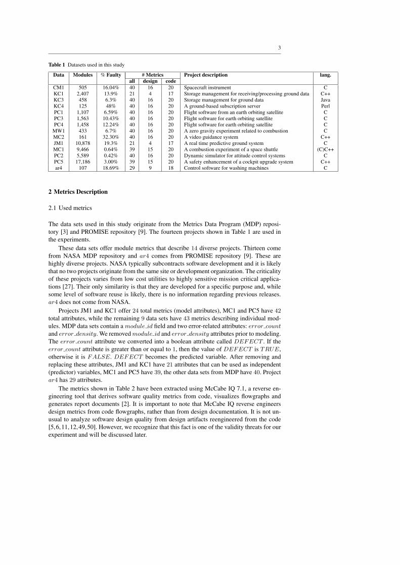
Table 1 Datasets used in this study

Data Modules % Faulty # Metrics Project description lang.all design code

CM1 505 16.04% 40 16 20 Spacecraft instrument CKC1 2,407 13.9% 21 4 17 Storage management for receiving/processing ground data C++KC3 458 6.3% 40 16 20 Storage management for ground data JavaKC4 125 48% 40 16 20 A ground-based subscription server PerlPC1 1,107 6.59% 40 16 20 Flight software from an earth orbiting satellite CPC3 1,563 10.43% 40 16 20 Flight software for earth orbiting satellite CPC4 1,458 12.24% 40 16 20 Flight software for earth orbiting satellite C

MW1 433 6.7% 40 16 20 A zero gravity experiment related to combustion CMC2 161 32.30% 40 16 20 A video guidance system C++JM1 10,878 19.3% 21 4 17 A real time predictive ground system CMC1 9,466 0.64% 39 15 20 A combustion experiment of a space shuttle (C)C++PC2 5,589 0.42% 40 16 20 Dynamic simulator for attitude control systems CPC5 17,186 3.00% 39 15 20 A safety enhancement of a cockpit upgrade system C++ar4 107 18.69% 29 9 18 Control software for washing machines C

2 Metrics Description

2.1 Used metrics

The data sets used in this study originate from the Metrics Data Program (MDP) reposi-tory [3] and PROMISE repository [9]. The fourteen projects shown in Table 1 are used inthe experiments.

These data sets offer module metrics that describe 14 diverse projects. Thirteen comefrom NASA MDP repository and ar4 comes from PROMISE repository [9]. These arehighly diverse projects. NASA typically subcontracts software development and it is likelythat no two projects originate from the same site or development organization. The criticalityof these projects varies from low cost utilities to highly sensitive mission critical applica-tions [27]. Their only similarity is that they are developed for a specific purpose and, whilesome level of software reuse is likely, there is no information regarding previous releases.ar4 does not come from NASA.

Projects JM1 and KC1 offer 24 total metrics (model attributes), MC1 and PC5 have 42total attributes, while the remaining 9 data sets have 43 metrics describing individual mod-ules. MDP data sets contain a module id field and two error-related attributes: error countand error density. We removed module id and error density attributes prior to modeling.The error count attribute we converted into a boolean attribute called DEFECT . If theerror count attribute is greater than or equal to 1, then the value of DEFECT is TRUE,otherwise it is FALSE. DEFECT becomes the predicted variable. After removing andreplacing these attributes, JM1 and KC1 have 21 attributes that can be used as independent(predictor) variables, MC1 and PC5 have 39, the other data sets from MDP have 40. Projectar4 has 29 attributes.

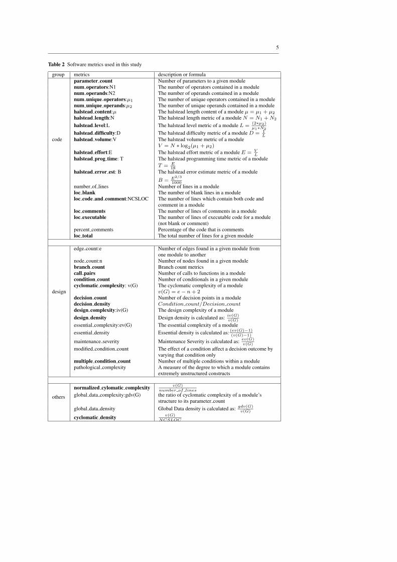
The metrics shown in Table 2 have been extracted using McCabe IQ 7.1, a reverse en-gineering tool that derives software quality metrics from code, visualizes flowgraphs andgenerates report documents [2]. It is important to note that McCabe IQ reverse engineersdesign metrics from code flowgraphs, rather than from design documentation. It is not un-usual to analyze software design quality from design artifacts reengineered from the code[5,6,11,12,49,50]. However, we recognize that this fact is one of the validity threats for ourexperiment and will be discussed later.

4

In all the data sets available metrics are classified into three groups: design, code, andother, as indicated in Table 2. What separates design metrics from code metrics is theopportunity to extract them from design specification diagrams such as UML. For exam-ple, Ohlsson and Alberg extract design metrics from Formal Description Language (FDL)graphs [43]. Their design metrics include node count, branch count, and McCabe cyclo-matic complexity measures [33], also produced by McCabe IQ tool. McCabe complexitymetrics are also used as design metrics in [56], the study that provides motivation and apoint of comparison for this research. As a quick reminder, if graph G represents module’sflowgraph, its cyclomatic complexity v(G) is calculated as v(G) = e−n +2, where e is thenumber of edges and n is the number of nodes.

The code metrics in our study are the features that can only be extracted from the sourcecode. Static code metrics, such as num operators, num operands, and Halstead metricsare calculated from program statements [19]. In this paper, other metrics are those relatedto both the design and code. Most data sets have four metrics we classified as other. We donot use other metrics in isolation to build models, but we include them in the experimentsin which fault prediction models are developed from all available attributes.

ar4 is the only data set that does not come from the MDP collection. This data sethas 29 attributes including nine design metrics, eighteen code metrics, and two metricsclassified as other. Although the names of some of the ar4 metrics are different fromMDP, they in fact are equivalent to a subset of metrics used in the MDP repository. Forexample, metrics “total loc”, “unique operands”, and “halstead time” in ar4 correspond to“loc total”,“num operands”, and “halstead prog time” in MDP. The metrics describing ar4project are presented in bold font in Table 2.

3 Experimental Design

As a reminder to readers, the goal of our experiments is support for the conjuncture thatthe incremental development of fault prediction models throughout the design and imple-mentation phases of the life cycle. There are two interesting aspects of incremental modeldevelopment:

1. Utilization of the increasing size of the training data set, and2. Timely (sequential) utilization of design and code metrics.

To reach these goals, we will compare the performance of models derived from:

– different percentages of data for model development (training): 10%, 25%, 50%, 75%,and 90%. In each experiment, the reminder of the data set will be used for model evalu-ation.

– different metric groups: design, code, and all.

The data sets we used do not include development schedule information. Therefore,we cannot faithfully emulate the actual “arrival” schedule of modules and their metrics.However, we will deploy cross-validation, the statistical practice of randomly partitioning asample of data into two subsets: training and testing subset ten times. Reporting the medianresult from the ten experiments should minimize the impact a development sequence couldhave on the prediction results. The predicted variable is DEFECT , that is, the models pre-dict whether a module is likely to contain fault(s). As mentioned earlier, we will deployfive well known classification algorithms for software quality prediction, listed in Table 3.These classification algorithms have consistently been recommended to practitioners and

5

Table 2 Software metrics used in this study

group metrics description or formula

code

parameter count Number of parameters to a given modulenum operators:N1 The number of operators contained in a modulenum operands:N2 The number of operands contained in a modulenum unique operators:µ1 The number of unique operators contained in a modulenum unique operands:µ2 The number of unique operands contained in a modulehalstead content:µ The halstead length content of a module µ = µ1 + µ2

halstead length:N The halstead length metric of a module N = N1 + N2

halstead level:L The halstead level metric of a module L = (2∗µ2)µ1∗N2

halstead difficulty:D The halstead difficulty metric of a module D = 1L

halstead volume:V The halstead volume metric of a moduleV = N ∗ log2(µ1 + µ2)

halstead effort:E The halstead effort metric of a module E = VL

halstead prog time: T The halstead programming time metric of a moduleT = E

18halstead error est: B The halstead error estimate metric of a module

B = E2/3

1000number of lines Number of lines in a moduleloc blank The number of blank lines in a moduleloc code and comment:NCSLOC The number of lines which contain both code and

comment in a moduleloc comments The number of lines of comments in a moduleloc executable The number of lines of executable code for a module

(not blank or comment)percent comments Percentage of the code that is commentsloc total The total number of lines for a given module

design

edge count:e Number of edges found in a given module fromone module to another

node count:n Number of nodes found in a given modulebranch count Branch count metricscall pairs Number of calls to functions in a modulecondition count Number of conditionals in a given modulecyclomatic complexity: v(G) The cyclomatic complexity of a module

v(G) = e− n + 2decision count Number of decision points in a moduledecision density Condition count/Decision countdesign complexity:iv(G) The design complexity of a moduledesign density Design density is calculated as: iv(G)

v(G)

essential complexity:ev(G) The essential complexity of a moduleessential density Essential density is calculated as: (ev(G)−1)

(v(G)−1)

maintenance severity Maintenance Severity is calculated as: ev(G)v(G)

modified condition count The effect of a condition affect a decision outcome byvarying that condition only

multiple condition count Number of multiple conditions within a modulepathological complexity A measure of the degree to which a module contains

extremely unstructured constructs

others

normalized cylomatic complexity v(G)number of lines

global data complexity:gdv(G) the ratio of cyclomatic complexity of a module’sstructure to its parameter count

global data density Global Data density is calculated as: gdv(G)v(G)

cyclomatic density v(G)NCSLOC

6

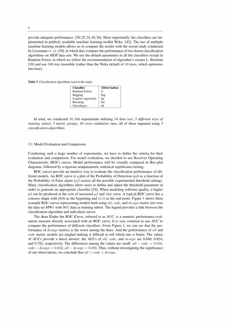
provide adequate performance [30,25,34,20,26]. More importantly, the classifiers are im-plemented in publicly available machine learning toolkit Weka [42]. The use of multiplemachine learning models allows us to compare the results with the recent study conductedby Lessmann et. al. [30], in which they compare the performance of two dozen classificationalgorithms on MDP data sets. We use the default parameters in all the classifiers except inRandom Forest, in which we follow the recommendation of algorithm’s creator L. Breiman[10] and use 500 tree ensemble (rather than the Weka default of 10 trees, which optimizesrun-time).

Table 3 Classification algorithms used in the study.

Classifier AbbreviationRandom Forest rfBagging bagLogistic regression lgiBoosting bstNaivebayes nb

In total, we conducted 10, 500 experiments utilizing 14 data sets, 5 different sizes oftraining subset, 3 metric groups, 10 cross validation runs, all of these repeated using 5classification algorithms.

3.1 Model Evaluation and Comparison

Conducting such a large number of experiments, we have to define the criteria for theirevaluation and comparison. For model evaluation, we decided to use Receiver OperatingCharacteristic (ROC) curves. Model performance will be visually compared in Box-plotdiagrams, followed by a rigorous nonparametric statistical significance testing.

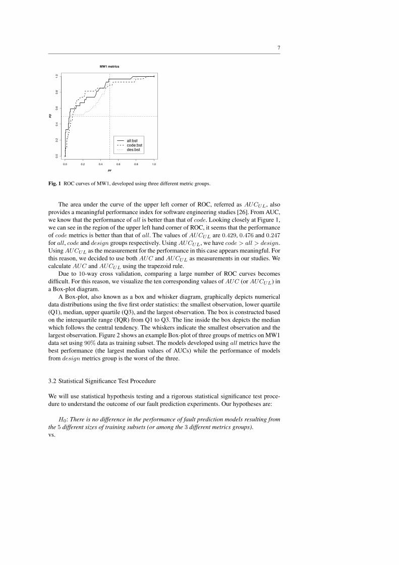
ROC curves provide an intuitive way to evaluate the classification performance of dif-ferent models. An ROC curve is a plot of the Probability of Detection (pd) as a function ofthe Probability of False alarm (pf ) across all the possible experimental threshold settings.Many classification algorithms allow users to define and adjust the threshold parameter inorder to generate an appropriate classifier [54]. When modeling software quality, a higherpd can be produced at the cost of increased pf and vice versa. A typical ROC curve has aconcave shape with (0,0) as the beginning and (1,1) as the end point. Figure 1 shows threeexample ROC curves representing models built using all, code, and design metric sets overthe data set MW1 with 90% data as training subset. The legend provides a link between theclassification algorithm and individual curves.

The Area Under the ROC Curve, referred to as AUC, is a numeric performance eval-uation measure directly associated with an ROC curve. It is very common to use AUC tocompare the performance of different classifiers. From Figure 1, we can see that the per-formance of design metrics is the worst among the three. And the performance of all andcode metric models are tangled making it difficult to tell which one is better. The valuesof AUCs provide a direct answer: the AUCs of all, code, and design are 0.840, 0.824,and 0.782, respectively. The differences among the values are small: all − code = 0.016,code− design = 0.042, all − design = 0.058. Thus, without investigating the significanceof our observations, we conclude that all > code > design.

7

0.0 0.2 0.4 0.6 0.8 1.0

0.0

0.2

0.4

0.6

0.8

1.0

MW1 metrics

PF

PD

all:bstcode:bstdes:bst

Fig. 1 ROC curves of MW1, developed using three different metric groups.

The area under the curve of the upper left corner of ROC, referred as AUCUL, alsoprovides a meaningful performance index for software engineering studies [26]. From AUC,we know that the performance of all is better than that of code. Looking closely at Figure 1,we can see in the region of the upper left hand corner of ROC, it seems that the performanceof code metrics is better than that of all. The values of AUCUL are 0.429, 0.476 and 0.247for all, code and design groups respectively. Using AUCUL, we have code > all > design.Using AUCUL as the measurement for the performance in this case appears meaningful. Forthis reason, we decided to use both AUC and AUCUL as measurements in our studies. Wecalculate AUC and AUCUL using the trapezoid rule.

Due to 10-way cross validation, comparing a large number of ROC curves becomesdifficult. For this reason, we visualize the ten corresponding values of AUC (or AUCUL) ina Box-plot diagram.

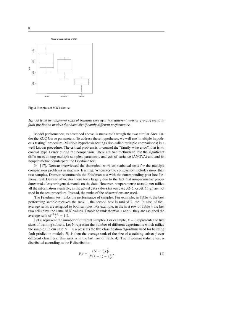
A Box-plot, also known as a box and whisker diagram, graphically depicts numericaldata distributions using the five first order statistics: the smallest observation, lower quartile(Q1), median, upper quartile (Q3), and the largest observation. The box is constructed basedon the interquartile range (IQR) from Q1 to Q3. The line inside the box depicts the medianwhich follows the central tendency. The whiskers indicate the smallest observation and thelargest observation. Figure 2 shows an example Box-plot of three groups of metrics on MW1data set using 90% data as training subset. The models developed using all metrics have thebest performance (the largest median values of AUCs) while the performance of modelsfrom design metrics group is the worst of the three.

3.2 Statistical Significance Test Procedure

We will use statistical hypothesis testing and a rigorous statistical significance test proce-dure to understand the outcome of our fault prediction experiments. Our hypotheses are:

H0: There is no difference in the performance of fault prediction models resulting fromthe 5 different sizes of training subsets (or among the 3 different metrics groups).vs.

8

all:bst code:bst des:bst

0.78

0.80

0.82

0.84

Three groups metrics of MW1

AUC

Fig. 2 Boxplots of MW1 data set

Hα: At least two different sizes of training subset(or two different metrics groups) result infault prediction models that have significantly different performance.

Model performance, as described above, is measured through the two similar Area Un-der the ROC Curve parameters. To address these hypotheses, we will use “multiple hypoth-esis testing” procedure. Multiple hypothesis testing (also called multiple comparisons) is awell-known procedure. The critical problem is to control the “family-wise error”, that is, tocontrol Type I error during the comparison. There are two methods to test the significantdifferences among multiple samples: parametric analysis of variance (ANOVA) and and itsnonparametric counterpart, the Friedman test.

In [17], Demsar overviewed the theoretical work on statistical tests for the multiplecomparisons problems in machine learning. Whenever the comparison includes more thantwo samples, Demsar recommends the Friedman test with the corresponding post-hoc Ne-menyi test. Demsar advocates these tests largely due to the fact that nonparametric proce-dures make less stringent demands on the data. However, nonparametric tests do not utilizeall the information available, as the actual data values (in our case AUC or AUCUL) are notused in the test procedure. Instead, the ranks of the observations are used.

The Friedman test ranks the performance of samples. For example, in Table 4, the bestperforming sample receives the rank 1, the second best is ranked 2, etc. In case of ties,average ranks are assigned to both samples. For example, in the first row of Table 4 the lasttwo cells have the same AUC values. Unable to rank them as 1 and 2, they are assigned theaverage rank of 1+2

2 = 1.5.Let k represent the number of different samples. For example, k = 5 represents the five

sizes of training subsets. Let N represent the number of different experiments which utilizethe samples. In our case N = 5 represents the five classification algorithms used for buildingfault prediction models. Rj is then the average rank of the size of a training subset j overdifferent classifiers. This rank is in the last row of Table 4). The Friedman statistic test isdistributed according to the F-distribution:

FF =(N − 1)χ2

F

N(k − 1)− χ2F

, (1)

9

Table 4 Comparison of fault prediction models on PC3 design metrics. The values inside the parenthesesare the ranks.

10% 25% 50% 75% 90%bag 0.66(5) 0.704(4) 0.733(3) 0.734(1.5) 0.734(1.5)bst 0.659(5) 0.698(4) 0.724(3) 0.728(2) 0.736(1)log 0.625(5) 0.704(4) 0.727(3) 0.734(2) 0.738(1)nb 0.635(5) 0.688(3) 0.682(4) 0.695(2) 0.703(1)rf 0.676(5) 0.694(4) 0.728(2) 0.721(3) 0.733(1)

rank 5.0 3.8 3.0 2.1 1.1

with k − 1 and (k − 1)(N − 1) degrees of freedom where χ2F = 12N

k(k+1) [ΣjR2j −

k(k+1)2

4 ].The critical value of F-distribution can be found in any statistical book.

If the null hypothesis of Friedman test is rejected, the Nemenyi test is further used as theafter-the-fact test. The performance of two samples is significantly different if their averageranks differ by at least the Critical Difference, denoted by CD:

CD = qα

√k(k + 1)

6N, (2)

where qα is the critical value of the Studentized range statistic divided by√

2, provided inDemsar’s paper [17].

The procedure is illustrated through an example as follows. Table 4 lists median valuesof AUC from models built from five different sizes as training subset(10%, 25%, 50%, 75%and 90%) using five classification algorithms using project PC3 design metrics. The rank ofeach cell is indicated inside the parenthesis along with the actual AUC value. The averagerank is listed in the last row. In the Friedman test, we use ranks instead of the actual values.

In this paper, we use the 95% confidence interval (α = 0.05) as a threshold to judgethe significance. The Friedman test and the Nemenyi test are implemented in the statisticalpackage R (http://www.r-project.org/). First, the Friedman test calculates the F distribution:χ2

F = 12∗55(5+1) [(5.02 + 3.82 + 3.02 + 2.12 + 1.12 − 5(5+1)2

4 )] = 18.12

FF =(5−1)χ2

F

5(5−1)−χ2F

= (5−1)∗18.125(5−1)−18.12 = 38.55.

With five training subsets and 5 classifiers, FF is distributed according to the F distributionwith 5 − 1 = 4 and (5 − 1)(5− 1) = 16 degrees of freedom. The critical value of F (4, 16)for α = 0.05 is 3.01. Because 3.01 < 38.55, we reject the null-hypothesis and conclude thatthere is significant difference among models developed from different sizes of the trainingdata on PC3. The critical value of qα is 2.728 [17], consequently:

CD = qα

√k(k+1)

6N = 2.728

√5(5+1)

6∗5 = 2.728.

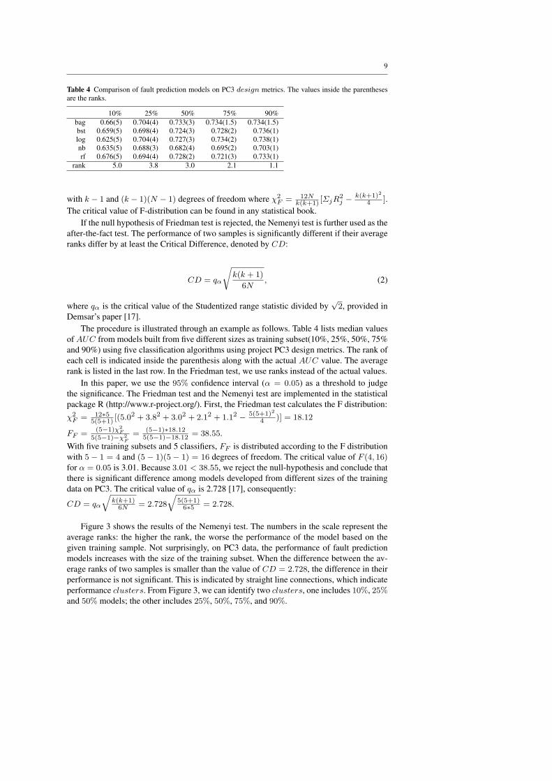
Figure 3 shows the results of the Nemenyi test. The numbers in the scale represent theaverage ranks: the higher the rank, the worse the performance of the model based on thegiven training sample. Not surprisingly, on PC3 data, the performance of fault predictionmodels increases with the size of the training subset. When the difference between the av-erage ranks of two samples is smaller than the value of CD = 2.728, the difference in theirperformance is not significant. This is indicated by straight line connections, which indicateperformance clusters. From Figure 3, we can identify two clusters, one includes 10%, 25%and 50% models; the other includes 25%, 50%, 75%, and 90%.

10

Fig. 3 Comparison of models which use different training subset sizes on PC3 design metrics, using Demsar’sprocedure.

4 Experimental Results

4.1 Increasing the Size of Training Set

One of the questions that repeatedly surfaces in discussions about fault prediction modelingdeals with the amount of data needed to build reasonably accurate models. The question isnot critical when models from earlier releases are used in the quality assurance of the newversion or product release. Presumably, such systems are part of the product line and faultprediction models from earlier releases are adequate for the new release [44]. However,when an organization develops one-of-a-kind system or the first system release with nosubstantial history (and limited reuse), the amount of data needed to develop the model isthe real issue in practice. This is certainly the case for most of the projects described in theNASA MDP repository. We will not directly address the ”minimal” data set requirementfor model development. Rather, following the idea of incremental model development, wewould like to know the rate of model improvement as additional modules and their metricsdescriptors become available.

For these reasons, we compare the performance of models generated using five trainingsubset, containing 10%, 25%, 50%, 75%, and 90% of project modules. Although these pro-portions represent different sizes of training data for different projects, they match realisticmilestones in the development life cycle.

We will test the following statistical hypotheses:H0: The size of the model’s training set has no influence on model performancevs.Hα: Some (at least two) models developed using different training subset sizes result insignificantly different model performance.

For this experiment, we utilize 14 data sets, 5 different training subsets, 3 groups ofmetrics, 5 classifiers and two measurement methods of AUC and AUCUL, summarized in420 box-plot diagrams. Each box-plot diagram reports the median result from 10 cross val-idation repetitions of each experiment. Due to the sheer volume of information, Demsar′s

11

statistical analysis procedure [17] will provide acceptable summarization of results. The re-sults are shown separately for models that utilize design metrics only, code metrics only,and all metrics.

The general trends to be reported are not surprising:

– 10% training subset results in the weakest performance.– In most cases, the “best” performance can be expected from models which use 90% of

data for training. Unfortunately, these models are the least useful as only 10% of themodules are left for fault prediction.

– Models increase their performance as the size of the training data set grows. However,these increases are rather minimal and statistical significance must be considered.

A more detailed analysis of the experimental results, including their statistical signifi-cance and practical implications follows.

4.1.1 Design metrics models

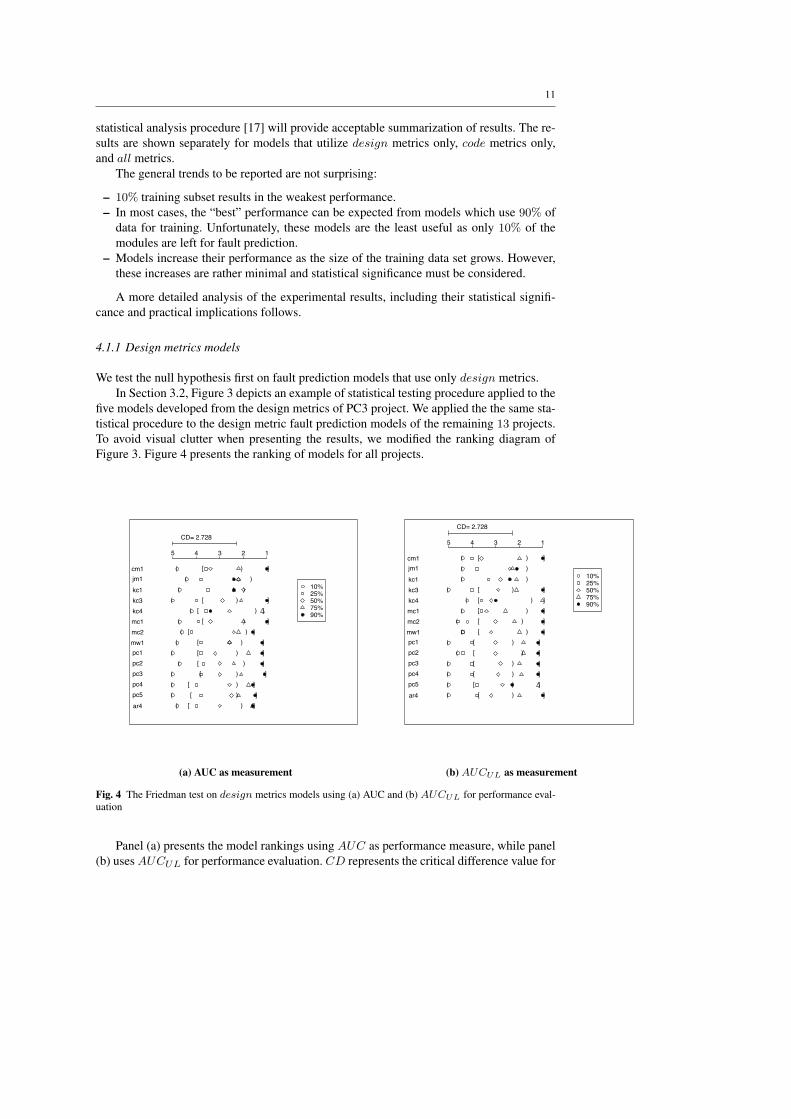
We test the null hypothesis first on fault prediction models that use only design metrics.In Section 3.2, Figure 3 depicts an example of statistical testing procedure applied to the

five models developed from the design metrics of PC3 project. We applied the the same sta-tistical procedure to the design metric fault prediction models of the remaining 13 projects.To avoid visual clutter when presenting the results, we modified the ranking diagram ofFigure 3. Figure 4 presents the ranking of models for all projects.

CD= 2.728

12345

cm1 )( [ ]jm1 )(kc1 )(kc3 )( [ ]kc4 )( [ ]mc1 )( [ ]mc2 )( [ ]mw1 )( [ ]pc1 )( [ ]pc2 )( [ ]pc3 )( [ ]pc4 )( [ ]pc5 )( [ ]ar4 )( [ ]

10%25%50%75%90%

CD= 2.728

12345

cm1 )( [ ]jm1 )(kc1 )(kc3 )( [ ]kc4 )( [ ]mc1 )( [ ]mc2 )( [ ]mw1 )( [ ]pc1 )( [ ]pc2 )( [ ]pc3 )( [ ]pc4 )( [ ]pc5 )( [ ]ar4 )( [ ]

10%25%50%75%90%

(a) AUC as measurement (b) AUCUL as measurement

Fig. 4 The Friedman test on design metrics models using (a) AUC and (b) AUCUL for performance eval-uation

Panel (a) presents the model rankings using AUC as performance measure, while panel(b) uses AUCUL for performance evaluation. CD represents the critical difference value for

12

this statistical test: if the difference between two ranks is greater than the value of CD, theyare statistically different, otherwise, they are not.

Referring to the graphic in Figure 4 the higher the rank (on a horizontal scale from 1 to5) the worse the performance of the model. To account for the statistical significance, weenclose the five models from each project into the two pairs of brackets. Each bracket pairencloses the distance equivalent to the value of CD = 2.728. The round brackets enclosemodels which form a performance cluster with the worst performing model (typically themodel which trains from the 10% subset). We will call this cluster the lower rank cluster.The square brackets enclose the performance cluster which includes the best performingmodel (typically inferred from the 90% subset). This will be our higher rank cluster. Thesebracket pairs replace the horizontal lines from Figure 3.

Let us look closely into the performance of the five models built from cm1 in Figure 4(a).For the increasing sizes of training subsets, the corresponding ranks are 4.8, 3.6, 3.4, 2.2,and 1. These ranks form two performance clusters. Models built from 25%, 50%, and 75%subsets are in the intersection between the lower and higher performance rank clusters. Thefault prediction models for projects jm1 and kc1 exhibit no statistically significant differ-ences regardless of the size of the training subset. Therefore, they are all included in a singleperformance rank cluster. The models for all other projects form two performance rank clus-ters. It is also interesting to note that in project kc4, the best performing model is developedusing 75% of modules for training. In smaller projects (kc4 contains only 125 modules),training from 90% may result in over-fitting.

The summary of design metrics based models evaluated through AUCUL, from Fig-ure 4(b), is similar:

1. In 2 data sets, jm1 and kc1, there is no significant difference amongst the 5 models.2. In 6 data sets the lower cluster includes models built from 10% to 50% of data. These

projects are kc3, pc1, pc2, pc3, pc4, ar4.3. In 4 data sets the lower cluster includes models built from 10% to 75% of data. These

projects are cm1, mc1, mc2, and mw1.4. In kc4 and pc5, models which used 75% of data for training ranked the best.5. In 3 data sets the higher cluster includes models built from 25% to 90% of data. These

projects are kc4, mc1, and pc5.6. In 9 data sets the higher cluster includes models built from 50% to 90% of data. These

projects are cm1, kc3, mc2, mw1, pc1, pc2, pc3, pc4, and ar4.

These results indicate that the model evaluation using AUC and AUCUL are, generally,very similar. Minor differences appear in average ranks and clustering, but they are not likelyto impact our conclusions. Further, there are never more than two performance clusters.Therefore, more detailed result comparisons in Table 5 and in Figure 5 will describe only10%, 50%, and 90% training subsets, and use AUC for model evaluation.

Table 5 shows median values of AUC and variances for 10%, 50%, and 90% train-ing subsets. The median value is rounded to two digits, variance to 4 digits. The last threecolumns show the percentage increase in model performance. If the performance increases,the value positive. Table 5 provides a closer look into the actual performance differencesbetween models. The gains in fault prediction vary from project to project and they are gen-erally difficult to anticipate. Clearly, the significance results indicate that building only oneor two models over the development life cycle, given that only design metrics are utilized,should be sufficient. Figure 5 visualizes the corresponding box-plot diagrams.

13

Table 5 Median and variance of 10%, 50%, and 90% training subset models from design metrics, measuredby AUC

data m10% v10% m50% v50% m90% v90%m50%m10%

− 1m90%m10%

− 1m90%m50%

− 1

cm1 0.54 0.0035 0.57 0.002 0.6 0.0133 5.56% 11.11% 5.26%jm1 0.66 9e-04 0.67 8e-04 0.66 0.0013 1.52% 0 -1.49%kc1 0.72 0.0027 0.73 9e-04 0.73 0.0028 1.39% 1.39% 0kc3 0.61 0.0194 0.74 0.0121 0.77 0.017 21.31% 26.23% 4.05%kc4 0.75 0.0109 0.78 0.0017 0.76 0.0175 4% 1.33% -2.56%mc1 0.53 0.0054 0.62 0.0091 0.68 0.0214 16.98% 28.3% 9.68%mc2 0.6 0.0087 0.63 0.0035 0.63 0.0271 5% 5% 0mw1 0.66 0.0163 0.76 0.0038 0.78 0.0282 15.15% 18.18% 2.63%pc1 0.57 0.0067 0.66 0.0028 0.69 0.0118 15.79% 21.05% 4.55%pc2 0.5 0.0269 0.67 0.0174 0.75 0.0503 34% 50% 11.94%pc3 0.65 0.0033 0.73 8e-04 0.73 0.0041 12.31% 12.31% 0pc4 0.73 0.0029 0.78 0.001 0.78 0.0036 6.85% 6.85% 0pc5 0.94 9e-04 0.95 1e-04 0.95 3e-04 1.06% 1.06% 0ar4 0.62 0.0185 0.7 0.0085 0.72 0.0803 12.9% 16.13% 2.86%

1 5 9

0.4

0.6

0.8

1.0

cm1

AUC

1 5 9

0.4

0.6

0.8

1.0

jm1

AUC

1 5 9

0.4

0.6

0.8

1.0

kc1

AUC

1 5 9

0.4

0.6

0.8

1.0

kc3AU

C

1 5 9

0.4

0.6

0.8

1.0

kc4

AUC

1 5 9

0.4

0.6

0.8

1.0

mc1

AUC

1 5 9

0.4

0.6

0.8

1.0

mc2

AUC

1 5 9

0.4

0.6

0.8

1.0

mw1

AUC

1 5 9

0.4

0.6

0.8

1.0

pc1

AUC

1 5 9

0.4

0.6

0.8

1.0

pc2

AUC

1 5 9

0.4

0.6

0.8

1.0

pc3

AUC

1 5 9

0.4

0.6

0.8

1.0

pc4

AUC

1 5 9

0.4

0.6

0.8

1.0

pc5

AUC

1 5 9

0.4

0.6

0.8

1.0

ar4

AUC

Fig. 5 Box-plots of 10%, 50%, and 90% training subset models built from design metrics, measured byAUC. On x-axis, “1” stands for 10%; “5” stands for 50%; “9” stands for 90%.

14

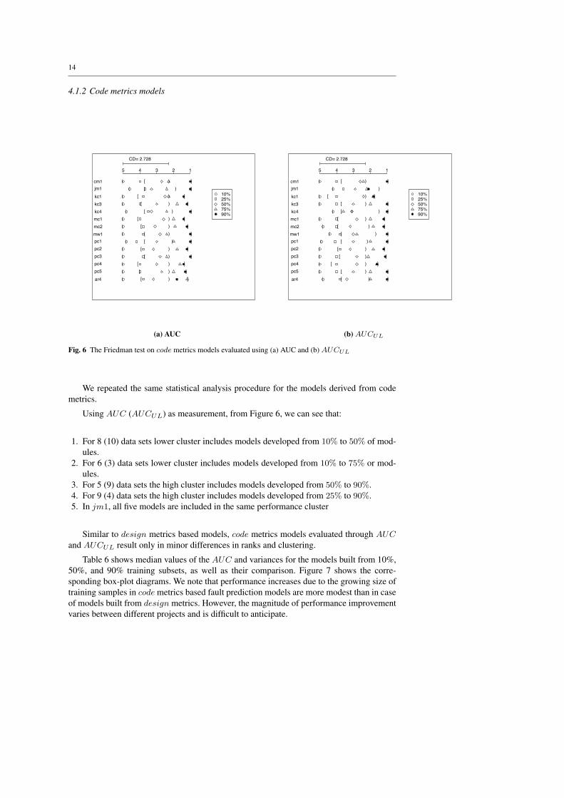
4.1.2 Code metrics models

CD= 2.728

12345

cm1 )( [ ]jm1 )( [ ]kc1 )( [ ]kc3 )( [ ]kc4 )( [ ]mc1 )( [ ]mc2 )( [ ]mw1 )( [ ]pc1 )( [ ]pc2 )( [ ]pc3 )( [ ]pc4 )( [ ]pc5 )( [ ]ar4 )( [ ]

10%25%50%75%90%

CD= 2.728

12345

cm1 )( [ ]jm1 )(kc1 )( [ ]kc3 )( [ ]kc4 )( [ ]mc1 )( [ ]mc2 )( [ ]mw1 )( [ ]pc1 )( [ ]pc2 )( [ ]pc3 )( [ ]pc4 )( [ ]pc5 )( [ ]ar4 )( [ ]

10%25%50%75%90%

(a) AUC (b) AUCUL

Fig. 6 The Friedman test on code metrics models evaluated using (a) AUC and (b) AUCUL

We repeated the same statistical analysis procedure for the models derived from codemetrics.

Using AUC (AUCUL) as measurement, from Figure 6, we can see that:

1. For 8 (10) data sets lower cluster includes models developed from 10% to 50% of mod-ules.

2. For 6 (3) data sets lower cluster includes models developed from 10% to 75% or mod-ules.

3. For 5 (9) data sets the high cluster includes models developed from 50% to 90%.4. For 9 (4) data sets the high cluster includes models developed from 25% to 90%.5. In jm1, all five models are included in the same performance cluster

Similar to design metrics based models, code metrics models evaluated through AUCand AUCUL result only in minor differences in ranks and clustering.

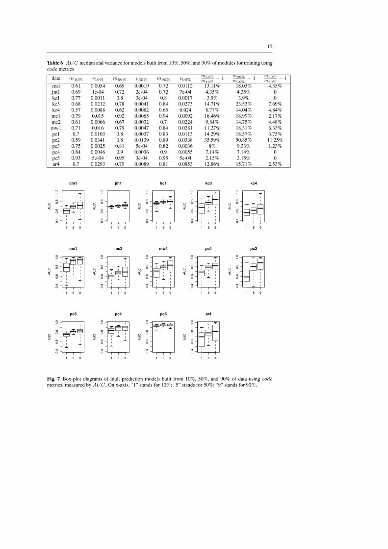
Table 6 shows median values of the AUC and variances for the models built from 10%,50%, and 90% training subsets, as well as their comparison. Figure 7 shows the corre-sponding box-plot diagrams. We note that performance increases due to the growing size oftraining samples in code metrics based fault prediction models are more modest than in caseof models built from design metrics. However, the magnitude of performance improvementvaries between different projects and is difficult to anticipate.

15

Table 6 AUC median and variance for models built from 10%, 50%, and 90% of modules for training usingcode metrics

data m10% v10% m50% v50% m90% v90%m50%m10%

− 1m90%m10%

− 1m90%m50%

− 1

cm1 0.61 0.0054 0.69 0.0019 0.72 0.0112 13.11% 18.03% 4.35%jm1 0.69 1e-04 0.72 2e-04 0.72 7e-04 4.35% 4.35% 0kc1 0.77 0.0011 0.8 3e-04 0.8 0.0017 3.9% 3.9% 0kc3 0.68 0.0212 0.78 0.0041 0.84 0.0273 14.71% 23.53% 7.69%kc4 0.57 0.0088 0.62 0.0082 0.65 0.024 8.77% 14.04% 4.84%mc1 0.79 0.015 0.92 0.0065 0.94 0.0092 16.46% 18.99% 2.17%mc2 0.61 0.0066 0.67 0.0032 0.7 0.0224 9.84% 14.75% 4.48%mw1 0.71 0.016 0.79 0.0047 0.84 0.0281 11.27% 18.31% 6.33%pc1 0.7 0.0103 0.8 0.0037 0.83 0.0113 14.29% 18.57% 3.75%pc2 0.59 0.0341 0.8 0.0139 0.89 0.0338 35.59% 50.85% 11.25%pc3 0.75 0.0025 0.81 5e-04 0.82 0.0036 8% 9.33% 1.23%pc4 0.84 0.0046 0.9 0.0036 0.9 0.0055 7.14% 7.14% 0pc5 0.93 5e-04 0.95 3e-04 0.95 5e-04 2.15% 2.15% 0ar4 0.7 0.0293 0.79 0.0089 0.81 0.0853 12.86% 15.71% 2.53%

1 5 9

0.4

0.6

0.8

1.0

cm1

AUC

1 5 9

0.4

0.6

0.8

1.0

jm1

AUC

1 5 9

0.4

0.6

0.8

1.0

kc1

AUC

1 5 9

0.4

0.6

0.8

1.0

kc3AU

C

1 5 9

0.4

0.6

0.8

1.0

kc4

AUC

1 5 9

0.4

0.6

0.8

1.0

mc1

AUC

1 5 9

0.4

0.6

0.8

1.0

mc2

AUC

1 5 9

0.4

0.6

0.8

1.0

mw1

AUC

1 5 9

0.4

0.6

0.8

1.0

pc1

AUC

1 5 9

0.4

0.6

0.8

1.0

pc2

AUC

1 5 9

0.4

0.6

0.8

1.0

pc3

AUC

1 5 9

0.4

0.6

0.8

1.0

pc4

AUC

1 5 9

0.4

0.6

0.8

1.0

pc5

AUC

1 5 9

0.4

0.6

0.8

1.0

ar4

AUC

Fig. 7 Box-plot diagrams of fault prediction models built from 10%, 50%, and 90% of data using codemetrics, measured by AUC. On x-axis, “1” stands for 10%; “5” stands for 50%; “9” stands for 90%.

16

CD= 2.728

12345

cm1 )( [ ]jm1 )(kc1 )( [ ]kc3 )( [ ]kc4 )( [ ]mc1 )( [ ]mc2 )( [ ]mw1 )( [ ]pc1 )( [ ]pc2 )( [ ]pc3 )( [ ]pc4 )( [ ]pc5 )( [ ]ar4 )( [ ]

10%25%50%75%90%

CD= 2.728

12345

cm1 )( [ ]jm1 )(kc1 )( [ ]kc3 )( [ ]kc4 )( [ ]mc1 )( [ ]mc2 )( [ ]mw1 )( [ ]pc1 )( [ ]pc2 )( [ ]pc3 )( [ ]pc4 )( [ ]pc5 )( [ ]ar4 )( [ ]

10%25%50%75%90%

(a) AUC as measurement (b) AUCUL as measurement

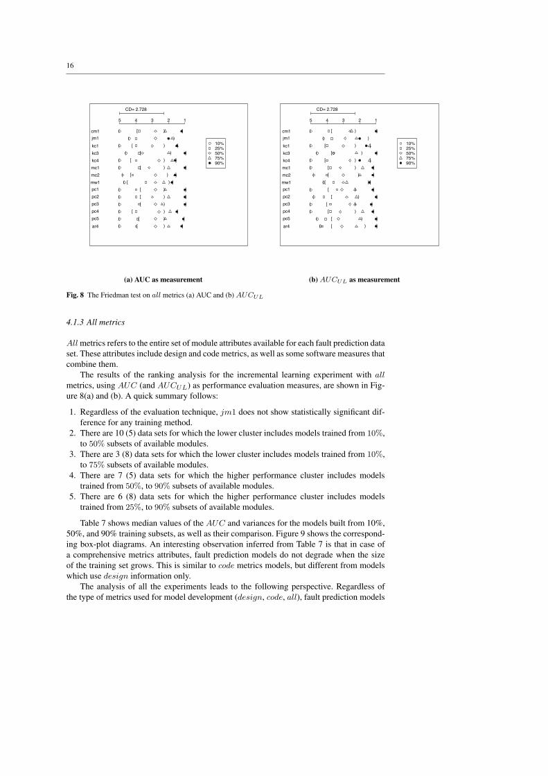
Fig. 8 The Friedman test on all metrics (a) AUC and (b) AUCUL

4.1.3 All metrics

All metrics refers to the entire set of module attributes available for each fault prediction dataset. These attributes include design and code metrics, as well as some software measures thatcombine them.

The results of the ranking analysis for the incremental learning experiment with allmetrics, using AUC (and AUCUL) as performance evaluation measures, are shown in Fig-ure 8(a) and (b). A quick summary follows:

1. Regardless of the evaluation technique, jm1 does not show statistically significant dif-ference for any training method.

2. There are 10 (5) data sets for which the lower cluster includes models trained from 10%,to 50% subsets of available modules.

3. There are 3 (8) data sets for which the lower cluster includes models trained from 10%,to 75% subsets of available modules.

4. There are 7 (5) data sets for which the higher performance cluster includes modelstrained from 50%, to 90% subsets of available modules.

5. There are 6 (8) data sets for which the higher performance cluster includes modelstrained from 25%, to 90% subsets of available modules.

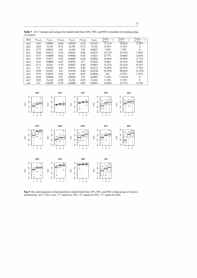
Table 7 shows median values of the AUC and variances for the models built from 10%,50%, and 90% training subsets, as well as their comparison. Figure 9 shows the correspond-ing box-plot diagrams. An interesting observation inferred from Table 7 is that in case ofa comprehensive metrics attributes, fault prediction models do not degrade when the sizeof the training set grows. This is similar to code metrics models, but different from modelswhich use design information only.

The analysis of all the experiments leads to the following perspective. Regardless ofthe type of metrics used for model development (design, code, all), fault prediction models

17

Table 7 AUC median and variance for models built from 10%, 50%, and 90% of modules for training usingall metrics

data m10% v10% m50% v50% m90% v90%m50%m10%

− 1m90%m10%

− 1m90%m50%

− 1

cm1 0.61 0.0054 0.69 0.0019 0.72 0.0112 13.11% 18.03% 4.35%jm1 0.69 1e-04 0.72 2e-04 0.72 7e-04 4.35% 4.35% 0kc1 0.77 0.0011 0.8 3e-04 0.8 0.0017 3.9% 3.9% 0kc3 0.68 0.0212 0.78 0.0041 0.84 0.0273 14.71% 23.53% 7.69%kc4 0.57 0.0088 0.62 0.0082 0.65 0.024 8.77% 14.04% 4.84%mc1 0.79 0.015 0.92 0.0065 0.94 0.0092 16.46% 18.99% 2.17%mc2 0.61 0.0066 0.67 0.0032 0.7 0.0224 9.84% 14.75% 4.48%mw1 0.71 0.016 0.79 0.0047 0.84 0.0281 11.27% 18.31% 6.33%pc1 0.7 0.0103 0.8 0.0037 0.83 0.0113 14.29% 18.57% 3.75%pc2 0.59 0.0341 0.8 0.0139 0.89 0.0338 35.59% 50.85% 11.25%pc3 0.75 0.0025 0.81 5e-04 0.82 0.0036 8% 9.33% 1.23%pc4 0.84 0.0046 0.9 0.0036 0.9 0.0055 7.14% 7.14%% 0pc5 0.93 5e-04 0.95 3e-04 0.95 5e-04 2.15% 2.15% 0ar4 0.7 0.0293 0.79 0.0089 0.81 0.0853 12.86% 15.71% 2.53%

1 5 9

0.4

0.6

0.8

1.0

cm1

AUC

1 5 9

0.4

0.6

0.8

1.0

jm1

AUC

1 5 9

0.4

0.6

0.8

1.0

kc1

AUC

1 5 9

0.4

0.6

0.8

1.0

kc3AU

C

1 5 9

0.4

0.6

0.8

1.0

kc4

AUC

1 5 9

0.4

0.6

0.8

1.0

mc1

AUC

1 5 9

0.4

0.6

0.8

1.0

mc2

AUC

1 5 9

0.4

0.6

0.8

1.0

mw1

AUC

1 5 9

0.4

0.6

0.8

1.0

pc1

AUC

1 5 9

0.4

0.6

0.8

1.0

pc2

AUC

1 5 9

0.4

0.6

0.8

1.0

pc3

AUC

1 5 9

0.4

0.6

0.8

1.0

pc4

AUC

1 5 9

0.4

0.6

0.8

1.0

pc5

AUC

1 5 9

0.4

0.6

0.8

1.0

ar4

AUC

Fig. 9 Box-plot diagrams of fault prediction models built from 10%, 50%, and 90% of data using all metrics,measured by AUC. On x-axis, “1” stands for 10%; “5” stands for 50%; “9” stands for 90%.

18

should be built as early as an initial set of modules becomes available. Using 10% of projectmodules for this purpose results in models that are statistically as good as those developedfrom 50% or sometimes even 75% of project modules. Larger training set generally helpsimprove model performance, but the cost of incremental model rebuilding should be com-pared with the performance benefits. When justified, model rebuilding does not need to bea continual or a frequent activity. Rather, models could be built early and, possibly, updatedat the mid point of the development.

These experiments further revealed that, in general, AUC and AUCUL offer similarperformance evaluation indices. For this reason, in the remaining experiments, we will onlyreport AUC.

4.2 Comparison of design, code, and all metrics models

The increase in size of available data for model definition is only one aspect in the incre-mental development of fault prediction models. The other opportunity comes from the factthat design artifacts and their metrics are typically available before the modules are imple-mented and code metrics can be computed. In rapid prototyping or agile processes, a fewmodules will be developed, implemented and tested in the first few process cycles. Theirfault proneness status can be used to build models predicting the quality of design or codeartifacts. Therefore, the question of comparing the performance of fault prediction modelsbuilt from different types of metrics is important.

To guide statistical analysis comparing design, code, and all metrics based models, wedefine the following hypotheses:H0: There is no difference in the performance of fault prediction of models developed usingthe three metrics groups.vs.Hα: Fault prediction models built from (at least) one of the three metrics groups offer sig-nificantly different performance.

The lesson learned in the previous section is that fault prediction models do not needfrequent updates. For this reason, we decided it will be sufficient to compare design, code,and all models built from 10% and 50% of the modules only.

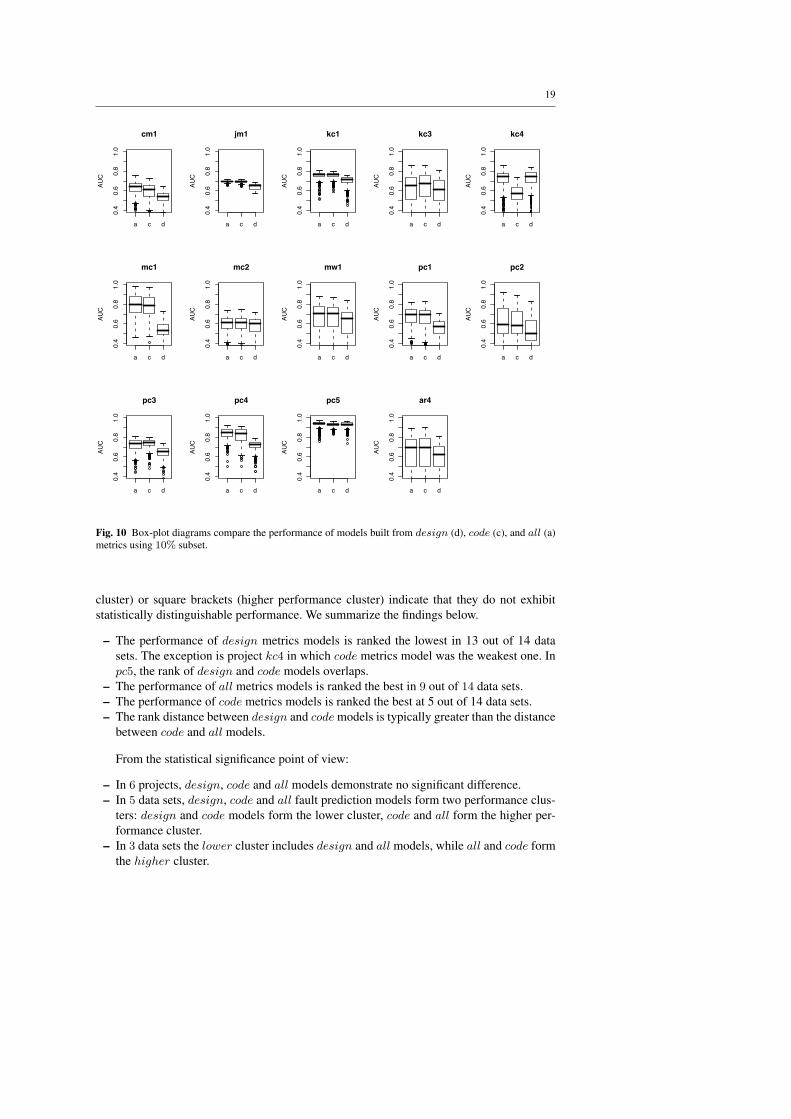
Figure 10 depicts box-plot diagrams for experiments with all the 14 data sets. The di-agrams compare the performance of models which use design, code, and all metrics builtfrom 10% subsets. The performance measure in these experiments is AUC. The box-plotsindicate that the majority of models built from all metrics outperform those built from codemetrics, which in turn outperform design metrics models. The statistical significance ofthese results will be tested following the Demsar’s procedure [17]. It is worth mention-ing here that the reported performance reflects models which use all five classification al-gorithms. While there are differences between classification algorithms, reporting medianAUC across all of them (following 10-way cross validation of each) minimizes the impactof the classifier and emphasizes the inherent properties of metrics data sets. We study theimpact of classification algorithms in the next section, but if Lessman’s results [30] arecorrect, models developed using different algorithms are not likely to have statistically sig-nificant performance differences.

Following the notation introduced earlier, Figure 11 introduces performance clustersbased on the value of the Critical Distance, which for this experiment assumes value CD =1.48. Enclosure of two or more models within either round brackets (lower performance

19

a c d

0.4

0.6

0.8

1.0

cm1

AUC

a c d

0.4

0.6

0.8

1.0

jm1

AUC

a c d

0.4

0.6

0.8

1.0

kc1

AUC

a c d

0.4

0.6

0.8

1.0

kc3

AUC

a c d

0.4

0.6

0.8

1.0

kc4

AUC

a c d

0.4

0.6

0.8

1.0

mc1

AUC

a c d

0.4

0.6

0.8

1.0

mc2

AUC

a c d

0.4

0.6

0.8

1.0

mw1

AUC

a c d

0.4

0.6

0.8

1.0

pc1

AUC

a c d

0.4

0.6

0.8

1.0

pc2

AUC

a c d

0.4

0.6

0.8

1.0

pc3

AUC

a c d

0.4

0.6

0.8

1.0

pc4

AUC

a c d

0.4

0.6

0.8

1.0

pc5

AUC

a c d

0.4

0.6

0.8

1.0

ar4

AUC

Fig. 10 Box-plot diagrams compare the performance of models built from design (d), code (c), and all (a)metrics using 10% subset.

cluster) or square brackets (higher performance cluster) indicate that they do not exhibitstatistically distinguishable performance. We summarize the findings below.

– The performance of design metrics models is ranked the lowest in 13 out of 14 datasets. The exception is project kc4 in which code metrics model was the weakest one. Inpc5, the rank of design and code models overlaps.

– The performance of all metrics models is ranked the best in 9 out of 14 data sets.– The performance of code metrics models is ranked the best at 5 out of 14 data sets.– The rank distance between design and code models is typically greater than the distance

between code and all models.

From the statistical significance point of view:

– In 6 projects, design, code and all models demonstrate no significant difference.– In 5 data sets, design, code and all fault prediction models form two performance clus-

ters: design and code models form the lower cluster, code and all form the higher per-formance cluster.

– In 3 data sets the lower cluster includes design and all models, while all and code formthe higher cluster.

20

CD= 1.48

123

cm1 ( )[ ]jm1 ( )[ ]

kc1 ( )

kc3 ( )[ ]

kc4 ( )[ ]

mc1 ( )[ ]

mc2 ( )

mw1 ( )pc1 ( )[ ]pc2 ( )pc3 ( )[ ]pc4 ( )[ ]pc5 ( )

ar4 ( )

descodall

Fig. 11 Statistical performance ranks of design, code, and all models built using 10% of data for training.

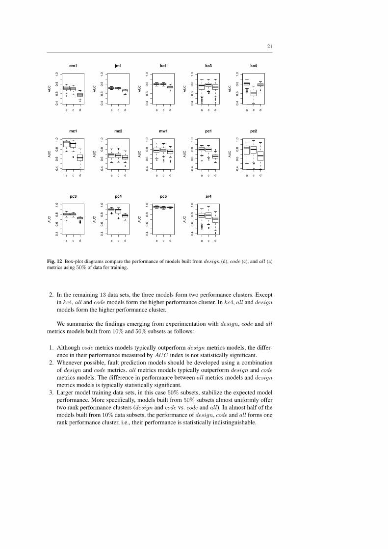
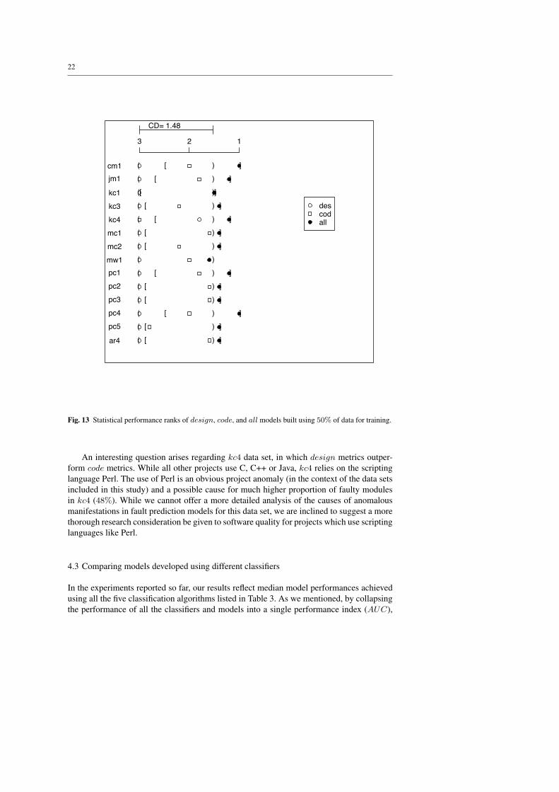
We repeated the same analysis using models built from 50% subsets of data sets. Thebox-plot diagrams are presented in Figure 12. The summary of the findings about modelsbuilt from 50% data subsets is very similar to those we had about models built from 10%subsets.

More interesting observations emerge from the diagram in Figure 13. Using 50% ofdata for model development seems to stabilize performance trends. For example, except inkc4, in all other data sets design metrics models offer the inferior performance. Even moreinterestingly, models built from all metrics outperform other models in all data sets. Pleasenote that this was not the case with models built from 10% of data, where in 5 projects codemodels outperformed those drawing from all metrics as attributes.

Further statistical analysis of models built from the 50% subsets reveals that:

1. Only one data set, mw1, offers design, code and all models with statistically indistin-guishable performance.

21

a c d

0.4

0.6

0.8

1.0

cm1

AUC

a c d

0.4

0.6

0.8

1.0

jm1

AUC

a c d

0.4

0.6

0.8

1.0

kc1

AUC

a c d

0.4

0.6

0.8

1.0

kc3

AUC

a c d

0.4

0.6

0.8

1.0

kc4

AUC

a c d

0.4

0.6

0.8

1.0

mc1

AUC

a c d

0.4

0.6

0.8

1.0

mc2

AUC

a c d

0.4

0.6

0.8

1.0

mw1

AUC

a c d

0.4

0.6

0.8

1.0

pc1

AUC

a c d

0.4

0.6

0.8

1.0

pc2

AUC

a c d

0.4

0.6

0.8

1.0

pc3

AUC

a c d

0.4

0.6

0.8

1.0

pc4

AUC

a c d

0.4

0.6

0.8

1.0

pc5

AUC

a c d

0.4

0.6

0.8

1.0

ar4

AUC

Fig. 12 Box-plot diagrams compare the performance of models built from design (d), code (c), and all (a)metrics using 50% of data for training.

2. In the remaining 13 data sets, the three models form two performance clusters. Exceptin kc4, all and code models form the higher performance cluster. In kc4, all and designmodels form the higher performance cluster.

We summarize the findings emerging from experimentation with design, code and allmetrics models built from 10% and 50% subsets as follows:

1. Although code metrics models typically outperform design metrics models, the differ-ence in their performance measured by AUC index is not statistically significant.

2. Whenever possible, fault prediction models should be developed using a combinationof design and code metrics. all metrics models typically outperform design and codemetrics models. The difference in performance between all metrics models and designmetrics models is typically statistically significant.

3. Larger model training data sets, in this case 50% subsets, stabilize the expected modelperformance. More specifically, models built from 50% subsets almost uniformly offertwo rank performance clusters (design and code vs. code and all). In almost half of themodels built from 10% data subsets, the performance of design, code and all forms onerank performance cluster, i.e., their performance is statistically indistinguishable.

22

CD= 1.48

123

cm1 ( )[ ]jm1 ( )[ ]

kc1 ( )[ ]

kc3 ( )[ ]

kc4 ( )[ ]

mc1 ( )[ ]

mc2 ( )[ ]

mw1 ( )pc1 ( )[ ]pc2 ( )[ ]pc3 ( )[ ]pc4 ( )[ ]pc5 ( )[ ]

ar4 ( )[ ]

descodall

Fig. 13 Statistical performance ranks of design, code, and all models built using 50% of data for training.

An interesting question arises regarding kc4 data set, in which design metrics outper-form code metrics. While all other projects use C, C++ or Java, kc4 relies on the scriptinglanguage Perl. The use of Perl is an obvious project anomaly (in the context of the data setsincluded in this study) and a possible cause for much higher proportion of faulty modulesin kc4 (48%). While we cannot offer a more detailed analysis of the causes of anomalousmanifestations in fault prediction models for this data set, we are inclined to suggest a morethorough research consideration be given to software quality for projects which use scriptinglanguages like Perl.

4.3 Comparing models developed using different classifiers

In the experiments reported so far, our results reflect median model performances achievedusing all the five classification algorithms listed in Table 3. As we mentioned, by collapsingthe performance of all the classifiers and models into a single performance index (AUC),

23

we intended to emphasize the inherent properties of metrics data sets. In this section, wereveal the performance impact of different classification algorithms.

A recent study by Lessmann et. al. [30] indicates that most classification algorithms donot offer models which exhibit statistically significant performance differences. Sixteen outof 19 algorithms included in their study belong to a ”higher” rank cluster. In addition to the10 data sets included in Lessmann’s study, we use four additional project data sets: mc1,mc2, pc5, and ar4. Out of the five classifiers in our study three (random forest, logistic re-gression and Naive Bayes) were reported by Lessmann to achieve statistically indistinguish-able performance. Further, Lessmann reports results only from all metrics models using 2

3of the data for training. We find some very interesting observations by experimenting withthe three types of metric sets (design, code, all) and by increasing the size of the trainingsubset (10% to 90%). An additional difference between the two studies reflects our opinionthat software quality practitioners are most likely to use off-the-shelf classifiers with theirdefault parameter values. We follow this principle in our study and report median resultsfrom 10-way cross validation. Lessmann et. al. use grid-search approach to find an opti-mal combination of algorithmic hyper-parameters which maximize the performance of eachclassifier and report the mean values of AUC.

Our statistical hypotheses for this experiment can be formulated as follows:H0: Fault prediction models developed from the same data sets using five different classifi-cation algorithms do not result in statistically different performance.vs.Hα: At least two classification algorithms provide models whose performance is signifi-cantly different.

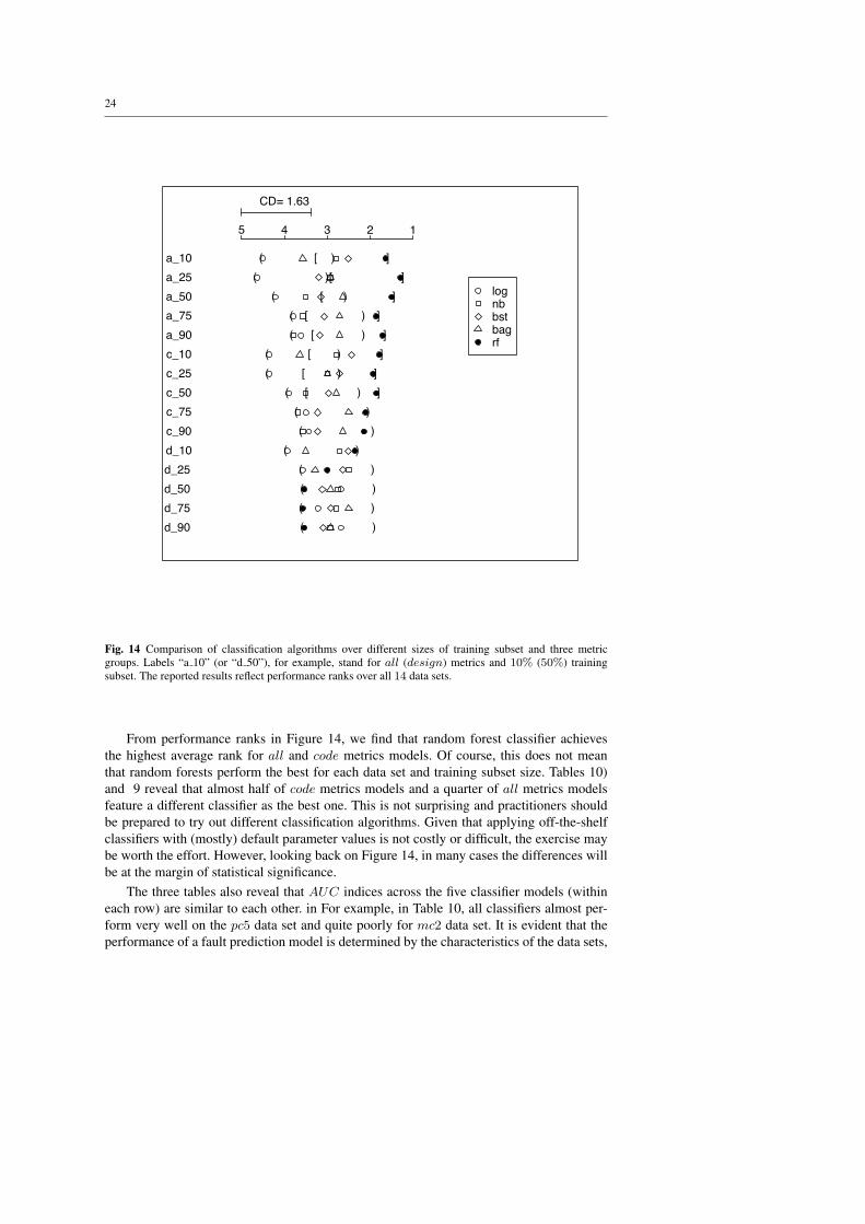
Figure 14 depicts the outcome of our experiments analyzed through Demsar’s proce-dure. The 15 experiments (lines in Figure 14) reflect the three metrics groups and the fivesizes of training subsets.

These results can be summarized as follows:

– Regardless of the classification algorithm, for all sizes of training subsets, models de-veloped from design metrics have statistically indistinguishable performance.

– For all sizes of training subsets, models developed from all metrics are grouped in twoperformance rank clusters; Random forest models are consistently in the higher rankcluster.

– Code metrics models fall in between. When trained on 10% to 50% of the data, theyresult in two rank clusters. When trained on larger subsets, all models fall into the singleperformance rank clusters.

These are very interesting insights. For all and code metrics models, we can infer thatthe choice of classification algorithm in mature data sets (those where we train from largersubsets), consistent with Lessmann’s results, matters less than when they are built early.When the samples come earlier in the development life cycle from a smaller number ofcompleted modules (10% or 25%), the choice of the classification algorithm matters more.

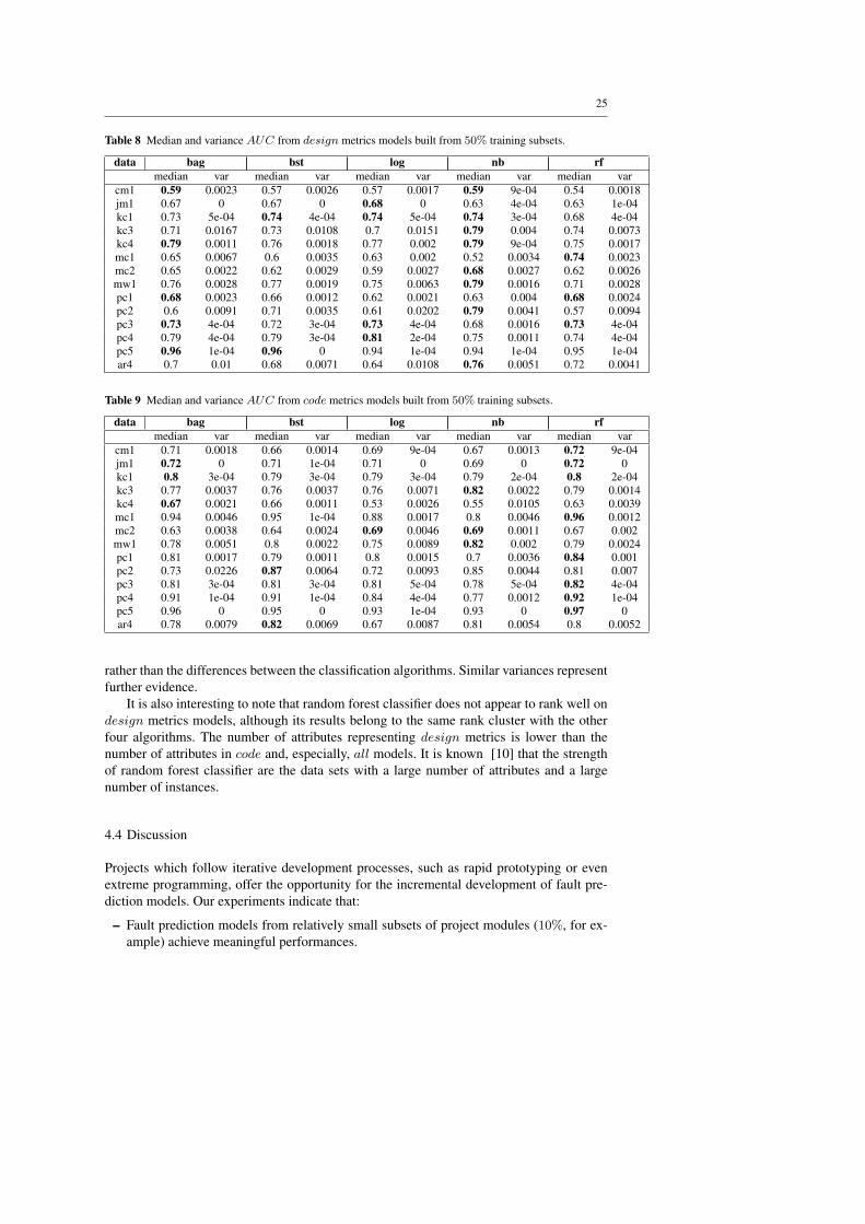
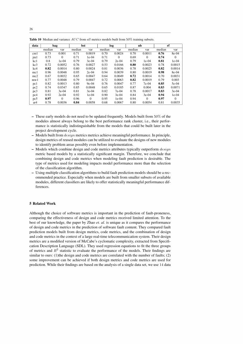
To gain better insights into these experiments, in Tables 8, 9, and 10 we preview medianAUC and variances from models developed for each data set. The top median AUC for eachproject is marked in bold. We decided to report these values from experiments in whichmodels are trained using 50% of the available data. Models build from 50% subsets arealmost always statistically similar to those developed from larger and smaller data subsets.These tables report the results which support box-plot diagrams shown in Figure 12. Thebox-plots do not differentiate the performance of five classification algorithms, while thetables do.

24

CD= 1.63

12345

a_10 )( [ ] a_25 )( [ ] a_50 )( [ ] a_75 )( [ ] a_90 )( [ ] c_10 )( [ ] c_25 )( [ ] c_50 )( [ ] c_75 )( c_90 )( d_10 )(d_25 )(d_50 )(d_75 )(d_90 )(

lognbbstbagrf

Fig. 14 Comparison of classification algorithms over different sizes of training subset and three metricgroups. Labels “a 10” (or “d 50”), for example, stand for all (design) metrics and 10% (50%) trainingsubset. The reported results reflect performance ranks over all 14 data sets.

From performance ranks in Figure 14, we find that random forest classifier achievesthe highest average rank for all and code metrics models. Of course, this does not meanthat random forests perform the best for each data set and training subset size. Tables 10)and 9 reveal that almost half of code metrics models and a quarter of all metrics modelsfeature a different classifier as the best one. This is not surprising and practitioners shouldbe prepared to try out different classification algorithms. Given that applying off-the-shelfclassifiers with (mostly) default parameter values is not costly or difficult, the exercise maybe worth the effort. However, looking back on Figure 14, in many cases the differences willbe at the margin of statistical significance.

The three tables also reveal that AUC indices across the five classifier models (withineach row) are similar to each other. in For example, in Table 10, all classifiers almost per-form very well on the pc5 data set and quite poorly for mc2 data set. It is evident that theperformance of a fault prediction model is determined by the characteristics of the data sets,

25

Table 8 Median and variance AUC from design metrics models built from 50% training subsets.

data bag bst log nb rfmedian var median var median var median var median var

cm1 0.59 0.0023 0.57 0.0026 0.57 0.0017 0.59 9e-04 0.54 0.0018jm1 0.67 0 0.67 0 0.68 0 0.63 4e-04 0.63 1e-04kc1 0.73 5e-04 0.74 4e-04 0.74 5e-04 0.74 3e-04 0.68 4e-04kc3 0.71 0.0167 0.73 0.0108 0.7 0.0151 0.79 0.004 0.74 0.0073kc4 0.79 0.0011 0.76 0.0018 0.77 0.002 0.79 9e-04 0.75 0.0017mc1 0.65 0.0067 0.6 0.0035 0.63 0.002 0.52 0.0034 0.74 0.0023mc2 0.65 0.0022 0.62 0.0029 0.59 0.0027 0.68 0.0027 0.62 0.0026mw1 0.76 0.0028 0.77 0.0019 0.75 0.0063 0.79 0.0016 0.71 0.0028pc1 0.68 0.0023 0.66 0.0012 0.62 0.0021 0.63 0.004 0.68 0.0024pc2 0.6 0.0091 0.71 0.0035 0.61 0.0202 0.79 0.0041 0.57 0.0094pc3 0.73 4e-04 0.72 3e-04 0.73 4e-04 0.68 0.0016 0.73 4e-04pc4 0.79 4e-04 0.79 3e-04 0.81 2e-04 0.75 0.0011 0.74 4e-04pc5 0.96 1e-04 0.96 0 0.94 1e-04 0.94 1e-04 0.95 1e-04ar4 0.7 0.01 0.68 0.0071 0.64 0.0108 0.76 0.0051 0.72 0.0041

Table 9 Median and variance AUC from code metrics models built from 50% training subsets.

data bag bst log nb rfmedian var median var median var median var median var

cm1 0.71 0.0018 0.66 0.0014 0.69 9e-04 0.67 0.0013 0.72 9e-04jm1 0.72 0 0.71 1e-04 0.71 0 0.69 0 0.72 0kc1 0.8 3e-04 0.79 3e-04 0.79 3e-04 0.79 2e-04 0.8 2e-04kc3 0.77 0.0037 0.76 0.0037 0.76 0.0071 0.82 0.0022 0.79 0.0014kc4 0.67 0.0021 0.66 0.0011 0.53 0.0026 0.55 0.0105 0.63 0.0039mc1 0.94 0.0046 0.95 1e-04 0.88 0.0017 0.8 0.0046 0.96 0.0012mc2 0.63 0.0038 0.64 0.0024 0.69 0.0046 0.69 0.0011 0.67 0.002mw1 0.78 0.0051 0.8 0.0022 0.75 0.0089 0.82 0.002 0.79 0.0024pc1 0.81 0.0017 0.79 0.0011 0.8 0.0015 0.7 0.0036 0.84 0.001pc2 0.73 0.0226 0.87 0.0064 0.72 0.0093 0.85 0.0044 0.81 0.007pc3 0.81 3e-04 0.81 3e-04 0.81 5e-04 0.78 5e-04 0.82 4e-04pc4 0.91 1e-04 0.91 1e-04 0.84 4e-04 0.77 0.0012 0.92 1e-04pc5 0.96 0 0.95 0 0.93 1e-04 0.93 0 0.97 0ar4 0.78 0.0079 0.82 0.0069 0.67 0.0087 0.81 0.0054 0.8 0.0052

rather than the differences between the classification algorithms. Similar variances representfurther evidence.

It is also interesting to note that random forest classifier does not appear to rank well ondesign metrics models, although its results belong to the same rank cluster with the otherfour algorithms. The number of attributes representing design metrics is lower than thenumber of attributes in code and, especially, all models. It is known [10] that the strengthof random forest classifier are the data sets with a large number of attributes and a largenumber of instances.

4.4 Discussion

Projects which follow iterative development processes, such as rapid prototyping or evenextreme programming, offer the opportunity for the incremental development of fault pre-diction models. Our experiments indicate that:

– Fault prediction models from relatively small subsets of project modules (10%, for ex-ample) achieve meaningful performances.

26

Table 10 Median and variance AUC from all metrics models built from 50% training subsets.

data bag bst log nb rfmedian var median var median var median var median var

cm1 0.73 0.001 0.71 0.0019 0.70 0.0024 0.70 0.0011 0.76 8e-04jm1 0.73 0 0.71 1e-04 0.71 0 0.69 0 0.74 0kc1 0.8 1e-04 0.79 3e-04 0.79 2e-04 0.79 1e-04 0.81 1e-04kc3 0.72 0.0052 0.76 0.0027 0.53 0.0166 0.80 0.0023 0.78 0.0015kc4 0.82 0.0014 0.80 0.0024 0.81 0.0036 0.78 0.0025 0.82 0.0014mc1 0.96 0.0048 0.95 2e-04 0.94 0.0039 0.80 0.0019 0.98 8e-04mc2 0.67 0.0032 0.65 0.0047 0.64 0.0049 0.72 0.0014 0.70 0.0031mw1 0.77 0.0048 0.79 0.0047 0.72 0.0063 0.82 0.0019 0.79 0.003pc1 0.82 0.0013 0.80 9e-04 0.76 0.0047 0.77 7e-04 0.85 5e-04pc2 0.74 0.0347 0.85 0.0048 0.65 0.0185 0.87 0.004 0.83 0.0071pc3 0.81 3e-04 0.81 3e-04 0.82 7e-04 0.78 0.0017 0.83 3e-04pc4 0.92 2e-04 0.92 1e-04 0.90 3e-04 0.84 3e-04 0.94 1e-04pc5 0.97 0 0.96 0 0.95 1e-04 0.94 0 0.97 0ar4 0.78 0.0036 0.84 0.0058 0.68 0.0067 0.80 0.0054 0.81 0.0035

– These early models do not need to be updated frequently. Models built from 50% of themodules almost always belong to the best performance rank cluster, i.e., their perfor-mance is statistically indistinguishable from the models that could be built later in theproject development cycle.

– Models built from design metrics metrics achieve meaningful performance. In principle,design metrics of reused modules can be utilized to evaluate the designs of new modulesto identify problem areas possibly even before implementation.

– Models which combine design and code metrics attributes typically outperform designmetric based models by a statistically significant margin. Therefore, we conclude thatcombining design and code metrics when modeling fault prediction is desirable. Thetype of metrics used for modeling impacts model performance more than the selectionof the classification algorithm.

– Using multiple classification algorithms to build fault prediction models should be a rec-ommended practice. Especially when models are built from smaller subsets of availablemodules, different classifiers are likely to offer statistically meaningful performance dif-ferences.

5 Related Work

Although the choice of software metrics is important in the prediction of fault-proneness,comparing the effectiveness of design and code metrics received limited attention. To thebest of our knowledge, the paper by Zhao et. al. is unique as it compares the performanceof design and code metrics in the prediction of software fault content. They compared faultprediction models built from design metrics, code metrics, and the combination of designand code metrics in the context of a large real-time telecommunication system. Their designmetrics are a modified version of McCabe’s cyclomatic complexity, extracted from Specifi-cation Description Language (SDL). They used regression equations to fit the three groupsof metrics and R2 statistic to evaluate the performance of the models. Their findings aresimilar to ours: (1)the design and code metrics are correlated with the number of faults; (2)some improvement can be achieved if both design metrics and code metrics are used forprediction. While their findings are based on the analysis of a single data set, we use 14 data

27

sets and our conclusions, based on sound statistical testing, indicate significant differencegained from the application of all metrics.

Menzies et. al. [36] select the “best” two or three attributes from 10 MDP data sets(the same data sets are included in our experiments). Halstead metrics, which we classify ascode metrics, appear on the list of “best” attributes much mode often than McCabe metrics(which we classify as design metrics). A study conducted by Xu et. al. [55] compare twelvemetrics are extracted from the Large Sky Area Multi Object Spectroscopic Telescope projectin China. They conclude that the most useful individual metrics for fault prediction areHalstead program difficulty, the number of executable statements, and Halstead programvolume. Cyclomatic complexity and related metrics fared low on their list. In these studies,Halstead metrics, part of our code metrics suite appear to be better predictors of fault contentthan the metrics from the McCabe group.

Requirement metrics have been used to predict fault prone software modules [24,25,32]. Malaiya et. al. examined the relationship between requirement changes and fault den-sity and found a positive correlation [32]. Javed et al. [24] investigate the impact of require-ment instability on software faults. In 4 industrial e-commerce projects and 30 releases theyfound: (1) a significant relationship between pre/post release change requests and overallsoftware faults; (2) insufficient and inadequate client communication during system designphase cause requirements changes and, consequently, software faults. Jiang and colleagues[25] found that combining requirements level metrics with code level metrics significantlyimproves the performance of fault prediction models.

One of the earliest studies of design metrics was conducted by Ohlsson and Alberg [43].They predicted fault-prone modules prior to coding in Telephone Switches system of 130modules at Ericsson Telecom AB. Their design metrics are derived from graphs where func-tions and subroutines in a module are represented by one or more graphs. These graphs,called Formal Description Language (FDL) graphs, offer a set of direct and indirect met-rics based on the measures of complexity. The examples of direct metrics are the number ofbranches, the number of graphs in modules, the number of possible connections in a graph,and the number of paths from input to the output signals etc. The indirect metrics are themetrics calculated from the direct metrics such as McCabe cyclomatic complexity, etc.

The suite of object oriented (OO) metrics, referred as CK metrics, has been first pro-posed by Chidamber and Kemerer [15]. They proposed six CK design metrics includingWeight Method Per Class (WMC), Number of Children (NOC), Depth of Inheritance Tree(DIT), Coupling Between Object class (CBO), Response For a Class (RFC), and Lack ofCohesion in Methods (LCOM). Basili et. al. [8] were among the first to validate these CKmetrics using 8 C++ systems developed by students. They demonstrated the benefits of CKmetrics over code metrics. In 1998, Chidamber, Darcy and Kemerer explored the relation-ship between the CK metrics and productivity, rework effort or design effort [14]. Theyshow that CK metrics have better explanatory power than traditional code metrics.

Predicting fault-prone software modules using metrics from design phase has recentlyreceived increased attention [46,57,37,48]. In these studies, metrics are either extractedfrom design documents or, like in our work, by mining the source code using the reverse en-gineering techniques. Subramanyam and Krishnan predict faults from three design metrics:Weight Method Per Class (WMC), Coupling Between Object Class (CBO), and Depth ofInheritance Tree (DIT) [48]. The system they study is a large B2C e-commerce applicationsuite developed using C++ and Java. They showed that these design metrics are significantlyrelated to defects and that defects are strongly related to the language used. Nagappan, Balland Zeller [37] predict component failures using OO metrics in five Microsoft softwaresystems. Their results show that these metrics are suitable to predict software defects. They

28

also show that the predictors are project specific, the suggestion also mentioned by Menzieset. al. [35].

Recovering design from source code has been a hot topic in software reverse engineering[12,6,5]. Systa [49] recovered UML diagrams from source code using static and dynamiccode analysis. Tonella and Potrich [50] were able to extract sequence diagrams from sourcecode. Briand et. al. demonstrated sequence diagrams, conditions and data flow can be re-verse engineered from Java code through transformation techniques [11].

Recently, Schroter, Zimmermann, and Zeller [46] applied reverse engineering to recoverdesign metrics from source code. They used 52 ECLIPSE plug-ins and found usage rela-tionships between these metrics and past failures. The relationship they investigate is theusage of import statements within a single release. The past failure data represents the num-ber of failures for a single release. They collected the data from version archives (CVS)and bug tracking systems (BUGZILLA). They built predictive models using the set of im-ported classes of each file as independent variables to predict the number of failures of thefile. The average prediction accuracy of the top 5% is approximately 90%. Zimmermann,Premraj and Zeller [57] further investigate ECLIPSE open source, extract object orientedmetrics along with static code complexity metrics and point out their effectiveness to pre-dict fault-proneness. Their data set is now posted in the PROMISE [9] repository. Neuhaus,Zimmermann, Holler and Zeller examine Mozilla code to extract the relationship of importsand function calls to predict software components’ vulnerabilities [41].

Besides requirement metrics, design metrics, and code metrics, various other measureshave been used to predict fault prone software modules. Historical project characteristic,developer information and social networks have all been reported as effective predictors.Ostrand, Weyuker, and Bell [44] predict the files most likely to contain the largest numbersof faults in the next release using modification history from previous release and the codein the current release. Illes-Seifert and Paech investigate the relationship between softwarehistory characteristics and the number of defects [23]. After analyzing 9 open source Javaprojects, they conclude that some history characteristics, such as the number of changes andthe number of distinct authors performing changes to a file, highly correlate with faults.Code churn, defined as the amount of code change taking place within a software unit [39],also called cached history [29], was also reported as an effective predictor of faults.

The role of developer social networks is currently receiving significant attention . Weyuker,Ostrand, and Bell [52] found that the addition of developer information improves theaccuracy of fault prediction models. Li et. al. analyzed 139 metrics collected from soft-ware product, development, deployment, usage, software and hardware configurations inOpenBSD [31]. They found that the number of messages to the technical discussion mailinglist during the development period is the best predictor of the number of field defects. Na-gappan et. al. [40] collect 8 organizational structure complexity metrics which relate codebinary to the organizational social networks, i.e, the number of engineers, the number ofex-engineers, edit frequency of source code, and organization intersection factors to predictfailure-proneness. They compare this model to models which use five groups of traditionalmetrics (code churn, code complexity, code coverage, dependency, and pre-release bugs).The use of organizational structure complexity metrics appears to hold a significant promisefor fault prediction.

29

6 Summary

The experiments reported in this paper have been motivated by the hypothesis that combin-ing software metrics from different stages in the development benefits the accuracy of faultprediction models. This motivation includes the utilization of different metrics types, thoseavailable from software design or code, as well as the proactive use of measurements fromsoftware modules for the development of fault prediction models when they become avail-able during project development. Publicly available NASA MDP and Promise repositoriesoffer a substantial number of data sets, 14 of which we have used in the experiments. Thelarge number of project data sets and a rigorous statistical test procedures we applied offerstrong evidence in support of our conclusions, presented below.

The starting position for our analysis of the relative strengths of design and code metricsin building fault prediction models comes from Zhao et. al. [56]. They claimed that designand code models perform comparatively well and that little improvement can be achievedif design and code metrics are jointly used in fault prediction. Our results confirm that theperformance of design and code models, measured through the area under the ROC curve, istypically statistically indistinguishable. In other words, although code metrics based modelsoutperform design metrics models, the performance margin is not statistically significant. Onthe other hand, the performance of models built from all metrics (which include design andcode metrics) typically outperform design models by a statistically significant margin. Ourexperiments, therefore, offer support for utilizing a combination of design and code metricsin building fault prediction models. However, if design metrics are available earlier, designmodels should not be discarded as they offer meaningful fault prediction performance.

The impact the size of the fault data set used for training has on model performance isalso significant and interesting. One of the basic questions regarding the practicality of faultprediction is: When does the project have sufficient amount of data to build a model? Beforewe describe our recommendations, it is necessary to mention that in many organizationsfault information from early (or earlier) product releases has been successfully used for faultprediction for the new release [44,52]. In organizations which practice software productlines or those where upgrades form the majority of project releases, data sufficiency is nota major problem. But there are many other organizations and projects which develop one-of-a-kind systems. Thirteen out of 14 data sets we analyzed come from such environments.These organizations must rely on the metrics from reused modules and those delivered andtested early in the development life cycle for building fault prediction models.

Most results from our experiments which test the impact of the training data size onthe fault prediction performance are not surprising. When derived from a larger data set,model performance improves. The interesting aspect of our results comes from statisticalhypothesis testing. In simple terms, the performance margin between models derived from50% data subsets and those derived from just 10% is not statistically significant. Further,models built from 50% data subsets and 90% data subsets typically belong the the sameperformance cluster too (but models built from 10% and 90% do not). The implication ofthis result is, we believe, very positive. Models developed from small data sets, presumablyearly in the project life time, offer fault prediction capability comparable with models thatcan only be developed much later. Therefore, while updating the fault prediction model is agood idea, it does not have to be practiced often. This conclusion offers the real chance tooptimize the cost of fault prediction model development. Fault prediction models, in turn,optimize the cost of verification and validation activities.

We believe the results from both experiments support the general hypothesis: defectdetectors can be improved by increasing the information content of the training set. There-

30

fore continuing to explore the effects of combining the attributes from multiple phases ofthe development life cycle, process and business related attributes, appears to be the mostpromising research direction [25,40,52].

In the third group of experiments, we examined the impact of the selection of the clas-sification algorithm in fault prediction modeling. In the recent paper, Lessmann [30] offersconvincing arguments that most classification algorithms offer statistically the same perfor-mance (i.e., their performance differences are not significant). One limitation of Lessmann’sanalysis is the uniform use of 2

3 of the data for model training. In our experiments we variedthe size of the training subset and the type of metrics used for training. We observed thatstatistically significant differences between classification algorithms do occur when modelsare developed from smaller training subsets. Further, significant differences are more likelyto occur when training from all and code metrics then from design metrics. Consequently,we recommend experimentation with several classification algorithms, recommended in theliterature (for example [30]) for fault prediction modeling.

Combined, the outcomes of our experiments provide a good guidance for an incrementalprocess for software fault prediction modeling. Models can be built early, from design met-rics and/or from relatively small subsets of available fault data. Updating such early modelsis recommended. The frequency of such updates can be optimized as model performancegains justify intermittent (sporadic) upgrades, rather than recurring ones.

We believe the results reported here have been obtained following a valid experimentalmethodology, using publicly available data sets. As any other experimental study we areaware of potential validity threats too. For example, we mentioned that the design metricsused in the experiments have been reengineered from the code. While in principle similarmetrics can (and have been) extracted from design documentation, it is likely that the metricsused in our experiments reflect the code more faithfully than the metrics collected at thedesign stage would. Had design models demonstrated better fault prediction performancethan code models, one could argue that any reduction in the code-level details from attributeswould have a tendency to improve performance. But, design models in our experiments donot perform as well as code models. Therefore, it seems logical that if design metrics do notreflect code structure as close as they do in our data sets, this would likely deteriorate theperformance even further. Without additional research, we cannot offer further assurances.

It is also worth repeating here that the data sets we analyzed do not contain informationabout when in the project development life time modules became available. To advocate in-cremental model development, we made the assumption that random selection of data subsetused for training (repeated 10 times in each experiment) represents a valid sample of mod-ules as if they became available before the modules we used for model evaluation. We areaware that software modules that become available early might suffer from quality deficien-cies which projects reduce as their processes mature. If fault introduction is reduced over thelife time of the project, our results about the suitability of fault prediction models built fromsmaller data subsets may be overly optimistic. Also, this might imply that updating modelsmore frequently during the project’s life time is warranted. Unfortunately, the data sets weuse do not allow us to study this problem further.

Lastly, we did not investigate the impact of feature selection on model performance.Feature selection algorithms minimize the number of attributes used in model developmentbased on some measure of their information content. Our experience with MDP datasetsindicates that a smaller number of attributes (metrics), typically a dozen or less, could offermodels that perform almost as well as the models which use the entire set of attributes[36]. This could have an impact on the effort invested in metrics collection. But, we havenever been able to develop a model from a reduced set of attributes which outperforms

31

models developed from comprehensive attribute sets. For this reason, we believe that featureselection is not likely to impact the validity of our results.

References

1. The R Project for Statistical Computing, available http://www.r-project.org/.2. Do-178b and McCabe IQ. available in http://www.mccabe.com/iq_research_whitepapers.htm.

3. Metric data program. NASA Independent Verification and Validation facility, available from http://MDP.ivv.nasa.gov.

4. S. H. Aljahdali, A. Sheta, and D. Rine. Prediction of software reliability: a comparison between regressionand neural network non-parametric models. ACS/IEEE International Conference on Computer Systems andApplications, pp: 25–29, June 2001.

5. G. Antoniol, G. Canfora, G. Casazza, A. D. Lucia, and E. Merlo. Recovering tracebility links betweencode and documentation. IEEE Transactions on Software Engineering, 28(10):970–983, 2002.

6. G. Antoniol, G. Casazza, M. Penta, and R. Fiutem. Object-oriented design patterns recovery. Journal ofSystems and Software, 59(2):181–196, 2001.

7. E. J. Barry, T. Mukhopadhyay, and S. A. Slaughter. Software Project Duration and Effort: An EmpiricalStudy. Inf. Tech. and Management,vol.3(1-2):113–136, 2002.

8. V. R. Basili, L. C. Briand, and W. L. Melo. A validation of object-oriented design metrics as qualityindicators, 1996.

9. G. Boetticher, T. Menzies and T. Ostrand. PROMISE Repository of empirical software engineering data.Available from http://promisedata.org/, 2007.

10. L. Breiman. Random forests. Machine Learning, 45:5–32, 2001.11. L. Briand, Y. Labiche, and J. Leduc. Toward the reverse engineering of uml sequence diagrams for

distributed java software. IEEE Transactions on Software Engineering, 32(9):642–663, 2006.12. G. CanforaHarman and M. D. Penta. New frontiers of reverse engineering. In FOSE ’07: 2007 Future

of Software Engineering, pages 326–341, Washington, DC, USA, 2007. IEEE Computer Society.13. V. U. Challagulla,F. B. Bastani, and I-Ling Yen, A Unified Framework for Defect Data Analysis Using

the MBR Technique. Proc. of the IEEE International Conference on Tools with Artificial Intelligence(ICTAI’06), pages 39–46, 2006,

14. S. R. Chidamber, D. P. Darcy, and C. F. Kemerer. Managerial use of metrics for object-oriented software:An exploratory analysis. IEEE Trans. Softw. Eng., 24(8):629–639, 1998.

15. S. R. Chidamber and C. F. Kemerer. A metrics suite for object oriented design. IEEE Trans. Softw. Eng.,20(6):476–493, 1994.

16. W. J. Conover. Practical Nonparametric Statistics. John Wiley and Sons, Inc., 1999.17. J. Demsar. Statistical comparisons of classifiers over multiple data sets. Journal of Machine Learning

Research, 7, 2006.18. N. E. Fenton and M. Neil, A Critique of Software Defect Prediction Models. IEEE Transactions on

Software Engineering, vol.25(5),pp 675–689,1999.19. N. E. Fenton, and S. L. Pfleeger, Software Metrics: A Rigorous & Practical Approach. PWS Publishing

Company,International Thompson Press, 1997.20. L. Guo, Y. Ma, B. Cukic, and H. Singh. Robust prediction of fault-proneness by random forests. In Proc.

of the 15th International Symposium on Software Relaibility Engineering ISSRE’04, pages 417–428, 2004.21. M. H. Halstead. Elements of Software Science. Elsevier, North-Holland, 1975,22. Y. Higo, K. Murao, S. Kusumoto, and K. Inoue. Predicting fault-prone modules based on metrics transi-

tions. DEFECTS ’08: Proceedings of the 2008 workshop on Defects in large software systems, pages:6–10,Seattle, Washington, 2008.

23. T. Illes-Seifert, B. Paech, Exploring the relationship of history characteristics and defect count: anempirical study. DEFECTS, pp 11-15, 2008.

24. T. Javed, M. E. Maqsood, and Q. S. Durrani. A study to investigate the impact of requirements instabilityon software defects. SIGSOFT Softw. Eng. Notes,29(3),pages 1–7, 2004.

25. Y. Jiang, B. Cukic, and T. Menzies. Fault prediction using early lifecycle data. The 18th IEEE Interna-tional Symposium on Software Reliability, ISSRE ’07.,pages 237–246, Nov. 2007.

26. Y. Jiang, B. Cukic, and Y. Ma. Techniques for Evaluating Fault Prediction Models. Empirical SoftwareEngineering, accepted for publication, 2008.

27. . Jiang, B. Cukic, and T. Menzies. Cost Curve Evaluation of Fault Prediction Models. The 19th IEEEInternational Symposium on Software Reliability, ISSRE ’08., Nov. 2007, (in print).

32

28. T. Khoshgoftaar, An Application of Zero-Inflated Poisson Regression for Software Fault Prediction.Proceedings of the 12th International Symposium on Software Reliability Engineering, ISSRE’01,pages66–73, Hong Kong, Nov. 2001.

29. S. Kim, T. Zimmermann, E. J. Whitehead Jr., and A. Zeller. Predicting Faults from Cached History. the29th International Conference on Software Engineering,ICSE’07,pages 489–498, May, 2007.

30. S. Lessmann, B. Baesens, C. Mues, and S. Pietsch. Benchmarking classification models for softwaredefect prediction: a proposed framework and novel findings. IEEE Trans. Softw. Eng., vol.34(4), July-Aug.pages:485–496, 2008.

31. P. L. Li, J. Herbsleb, and M. Shaw. Finding Predictors of Field Defects for Open Source SoftwareSystems in Commonly Available Data Sources: A Case Study of OpenBSD. METRICS ’05: Proceedingsof the 11th IEEE International Software Metrics Symposium, pages:32, Sept. 19-22, 2005.

32. Y. Malaiya and J. Denton. Requirement volatility and defect density. Proc. International Symposium onSoftware Reliability Engineering ISSRE’99, pages 285–294, Nov. 1999.

33. T. J. McCabe. A Complexity Measure. IEEE Trans. Softw. Eng., vol.2(4):308–320, Dec. 1976.34. T. Menzes, B. Turhan, A. Bener, G. Gay, B. Cukic, and Y. Jiang. Implications of ceiling effects in defect

predictors. PROMISE 2008.35. T. Menzies, J. DiStefano, A. Orrego, and R. Chapman. Assessing predictors of software defects. In

Proceedings, workshop on Predictive Software Models, Chicago, 2004.36. T. Menzies, J. Greenwald, and A. Frank. Data mining static code attributes to learn defect predic-

tors. IEEE Transactions on Software Engineering, 33(1):2–13, January 2007. Available from http://menzies.us/pdf/06learnPredict.pdf.

37. N. Nagappan, T. Ball, and A. Zeller. Mining metrics to predict component failures. In ICSE ’06:Proceeding of the 28th international conference on Software engineering, pages 452–461, New York, NY,USA, 2006. ACM Press.

38. N. Nagappan, T. Ball, and B. Murphy. Using Historical Data and Product Metrics for Early Estimationof Software Failures. ISSRE’06, Raleigh, NC, pages 62–71, 2006.

39. N. Nagappan, and T. Ball. Use of Relative Code Churn Measures to Predict System Defect Density. the27th International Conference on Software Engineering, ICSE’05, pages 284–292, May, 2005.

40. N. Nagappan, B. Murphy, and V. Basili. The influence of organizational structure on software quality: anempirical case study. ICSE ’08: Proceedings of the 30th international conference on Software engineering,Leipzig, Germany, 2008.

41. S. Neuhaus, T. Zimmermann, C. Holler, and A. Zeller. Predicting vulnerable software components.Alexandria, Virginia, USA, 2007. CCS’07.

42. U. of Waikato. Weka software package. The University of Waikato, available http://www.cs.waikato.ac.nz/ml/weka/.

43. N. Ohlsson and H. Alberg. Predicting fault-prone software modules in telephone switches. IEEE Trans-actions on Software Engineering, 22(12):886–894, 1996.

44. T.J. Ostrand, E.J. Weyuker, and R. M. Bell. Predicting the location and number of faults in large softwaresystems. IEEE Trans. Softw. Eng. 31(4):340–355, 2005.

45. N. F. Schneidewind, Investigation of Logistic Regression as a Discriminant of Software Quality. Pro-ceedings of the 7th International Software Metrics Symposium, pages 328–337, London,Apr. 2001.

46. A. Schroter, T. Zimmermann, and A. Zeller. Predicting component failures at design time. In ISESE ’06:Proceedings of the 2006 ACM/IEEE international symposium on International symposium on empiricalsoftware engineering, pages 18–27, New York, NY, USA, 2006. ACM Press.

47. S. Siegel. Nonparametric Satistics. New York: McGraw- Hill Book Company, Inc., 1956.48. R. Subramanyam and M. S. Krishnan. Empirical analysis of ck metrics for object-oriented design com-

plexity: Implications for software defects. IEEE Trans. Softw. Eng., 29(4):297–310, 2003.49. T. Systa. Static and dynamic reverse engineering techniques for Java software systems. PhD thesis,

2000.50. P. Tonella and A. Potrich. Reverse engineering of object oriented code. Springer-Verlag, Berlin, Heidel-

berg, New York, 2005.51. A. V. Lamsweerde. Requirements engineering in the year 00: a research perspective. International

Conference on Software Engineering, pages 5–19, 2000.52. E. J. Weyuker, T. J. Ostrand, and R. M. Bell. Using Developer Information as a Factor for Fault Predic-

tion. PROMISE ’07: Proceedings of the Third International Workshop on Predictor Models in SoftwareEngineering,Washington, DC, USA, pages:8,2007

53. Chadd C. Williams, Jeffrey K. Hollingsworth. Automatic Mining of Source Code Repositories to Im-prove Bug Finding Techniques. IEEE Trans. Softw. Eng., 31(6):466–480,2005.

54. I. H. Witten and E. Frank. Data Mining: Practical machine learning tools and techniques. MorganKaufmann, Los Altos, US, 2005.

33

55. Z. Xu, X. Zheng, and P. Guo. Empirically Validating Software Metrics for Risk Prediction Based onIntelligent Methods. ISDA (1), pages 1049–1054,2006.

56. M. Zhao, C. Wohlin, N. Ohlsson, and M. Xie. A comparison between software design and code metricsfor the prediction of software fault content. Information and Software Technology, 40(14):801–809, 1998.

57. T. Zimmermann, R. Premraj, and A. Zeller. Predicting defects for eclipse. In PROMISE’07: InternationalWorkshop on ICSE Workshops 2007, pages 9–9, May 2007.