incumbency disadvantage in weak party systems: evidence...
TRANSCRIPT

Incumbency Disadvantage In Weak PartySystems: Evidence from Brazil∗
Marko Klasnja † Rocıo Titiunik‡
PhD Candidate Assistant ProfessorNew York University University of Michigan
November 6, 2013
Preliminary (and Incomplete) Draft
Abstract
We study the incumbency advantage of political parties in Brazil’s municipal mayorelections using a regression discontinuity design. Comparing municipalities where aparty barely lost the mayor elections to municipalities where it barely won, we findevidence of a strong negative effect on the probability of winning in the following elec-tion. We propose an explanation for these findings that focuses on the interaction ofBrazil’s weak political parties, the personalistic nature of political networks, and theinstitutional constraints on electoral horizons. Our explanation yields predictions thatwe are able to corroborate empirically in an analysis that conditions on whether thepreviously elected incumbent is running for reelection.
Keywords: Incumbency advantage, regression discontinuity, Brazilian politics
∗We thank Henry Brady, Matıas Cattaneo, Don Green, Jas Sekhon and Eric Schickler, Jonathan Wandand seminar participants at the University of Michigan for valuable comments and discussions. We aregrateful to Humberto Dantas for sharing data with us. This research was in part supported by the Institutefor Business and Economic Research, U.C. Berkeley. This manuscript is a substantially revised version ofthe paper “Incumbency Advantage in Brazil: Evidence from Municipal Mayor Elections” (first draft: March30, 2009).†Wilf Family Department of Politics, New York University 19 W. 4th St, Second Floor. New York, NY
10012. Email: <[email protected]>, Web: https://files.nyu.edu/mk3296/public/.‡Department of Political Science, 505 South State St., 5700 Haven Hall, University of Michigan, Ann
Arbor, MI 48109. Email: <[email protected]>, Web: http://www.umich.edu/~titiunik.

1 Introduction
A vast number of scholars have argued that incumbent legislators in the United States enjoy
a substantial electoral advantage over challengers who dispute their seats.1 This advantage
is attributed to a variety of different factors, including the ability of incumbents to deter
high-quality challengers, their exclusive access to direct perquisites of office such as franking
privileges, name recognition and means to perform constituency service, and the ability of
incumbency to function as a cue when partisan ties are weak. The literature on incumbency
advantage mostly focuses on the personal advantage of incumbent legislators, but recent
work by Lee (2008) has shown that this advantage extends also to parties.
The arguments and evidence for the U.S. have contributed to the idea that being an
incumbent is intrinsically advantageous, emphasizing the access to resources to mobilize
and please the electorate that incumbency brings to both parties and politicians. But in
a context of weak parties, personalistic political networks and institutional constraints on
electoral horizons, the effects of incumbency may become more complex, and incumbency
may result in electoral losses.
Although the evidence is scarce, the few scholars who have studied incumbency effects in
developing countries have failed to find a positive effect of incumbency on electoral outcomes.
Linden (2004) and Uppal (2009) estimate incumbency effects in India’s parliamentary elec-
tions at the national and state level, respectively, and find a negative incumbency advantage,
i.e. an incumbency disadvantage. These results have been subsequently confirmed by Aidt
et al. (2011) and Fisman et al. (2012). Miguel and Zahidi (2004) estimate incumbency ef-
fects in national parliamentary elections in Ghana and find negative but insignificant effects
on both the vote share and the probability of winning in the following election. All these
1The list is too long for an exhaustive enumeration. The studies include Alford and Brady (1989),Ansolabehere et al. (1988), Ansolabehere et al. (2000), Cox and Katz (1996), Cox and Morgenstern (1993),Erikson (1971), Erikson (1972), Ferejohn (1977), Fiorina (1977), Gelman and King (1990), Jacobson (1987),Krehbiel and Wright (1983), and Levitt and Wolfram (1997). See Ansolabehere and Snyder (2002) for astudy that also considers executive offices.
2
studies use a regression discontinuity design. In addition, while not using the regression dis-
continuity design or focusing explicitly on incumbency advantage, scholars have shown that
an overwhelming majority of coalition governments in democracies in central and eastern
Europe have failed to win reelection since the fall of communism (Birch 2003; Roberts 2008;
Pop-Eleches 2010).
This paper contributes to the study of incumbency effects in developing countries by
analyzing Brazil’s municipal mayor elections using a regression discontinuity design. It is
well known that estimating the effects of incumbency poses great methodological challenges
due to the reciprocal causation between incumbency status and political skills broadly un-
derstood. Lee (2008) formally justified using regression discontinuity to estimate the in-
cumbency advantage of a party when there is a random chance element to the actual vote
share obtained in the elections. We apply this design to study the incumbency effect for
Brazil’s three largest political parties at the municipal level: Partido do Movimento Demo-
cratico Brasileiro (PMDB), Democratas (DEM, formerly Partido da Frente Liberal, PFL)
and Partido da Social Democracia Brasileira (PSDB). By comparing municipalities where a
given party barely lost to municipalities where it barely won in the 2000, 2004, 2008 and 2012
elections, we find evidence of a negative effect of incumbency on the probability of winning
in the following election. The results are robust to different specifications, and observable
pre-treatment characteristics show no evidence of a jump at the discontinuity, as expected
under a valid RD design.
Our contribution is twofold. First, we show that, as measured by the RD estimand, the
incumbency advantage in Brazil’s mayor elections is negative: when a party barely wins
the mayor election, it is significantly less likely to win the following election. This negative
effect is observed for the three largest parties considered when all elections are pooled in a
single analysis, and in three out of the four election pairs when the analysis is disaggregated.
The effect also holds (pooling and disaggregating) when we define the effect for the parties
simultaneously, focusing on the incumbency advantage for the incumbent party. In sum, our
3

results show that the RD-based incumbency advantage is persistently negative in Brazil’s
mayor elections.
Our second contribution, which is currently in progress, is to develop and test an ex-
planation for the negative incumbency advantage phenomenon. Our explanation focuses on
Brazil’s weak political parties, and their interaction with the presence of term limits (mayors
are elected for four years and can only serve two consecutive terms). Our hypothesis is that,
in the election immediately after term-limited mayors are forced to retire, the mayor’s party
suffers electoral losses due to either the loss of the mayor’s network and reputation or the
mayor’s undesirable behavior in his last term, for which voters punish his party. Our final
goal is to distinguish which of these explanations is true. For now, we show a conditional
RD analysis that is consistent with our prediction that the incumbency disadvantage should
be concentrated in municipalities where mayors were term limited.
The rest of the paper is organized as follows. Section 2 discusses Brazil’s institutional
background. Section 3 presents the methodology. Section 4 briefly explains the data sources,
and Section 5 presents the main results. Section 6 provides a preliminary attempt at devel-
oping an explanation of the results. We conclude briefly in Section 7.
2 Institutional Background
Scholars have long emphasized two fundamental features of Brazil’s political system: a very
strong federalism and a weakly institutionalized party system. In this section, we provide a
brief overview of Brazil’s institutional background with an emphasis on these two features,
which we believe are important for an adequate interpretation of the results presented in
Section 5.
When Brazil’s Old Republic was founded in 1891, a highly decentralized federal system
was put in place. In this early period, known as the “Politics of the Governors”, state gov-
ernors decisively dominated the country’s politics (Samuels 2004). Although the military
government of 1930–1945 sought to debilitate local governments and impose a strong cen-
4

tral authority, the power of the states was never completely dismantled, and by the time
democracy returned in 1945 it was clear that governors were crucial players in the political
arena. States recovered a crucial position in the relationship between the national execu-
tive and the national legislature: having access to substantial resources, governors exerted
influence over national legislators elected from their state, for whom access to the state net-
works of patronage was crucial to advance their political careers (Abrucio 1998; Samuels
2002). The military regime installed in 1964 tried to undermine these state-based support
networks but ultimately failed (Samuels 2004), and states entered Brazil’s latest democratic
experience in 1989 with remarkable autonomy and high influence on the national political
scene.2 Governors continue to be considered the “power brokers” in Brazil’s legislative and
distributive politics, due to their influence on their state’s Congressional delegations through
broad clientelistic networks and their control of nominations to most important offices, and
their overall control of state-level politics via pork-barrel funds (Ames 2001a; Abrucio 1998;
Carey and Reinhardt 2001; Montero 2005; Samuels and Abrucio 2000; Samuels 2002)
The political power of municipalities was much more limited in the pre-1964 period, but
this situation gradually changed during the 1970s and 1980s. Samuels (2000b, 2004) has
argued that the continuation of direct elections in a large number of municipalities during
the military regime together with the interruption of the states’ intermediary role between
the national executive and municipal governments, gradually contributed to an increase in
municipal political autonomy during the military regime. In particular, these limitations in
the intermediary role of states led to an increase in the political capital of municipal mayors,
who were the politicians most clearly able to claim credit for the implementation of projects
at the local level.
This gradual increase in municipal decentralization and autonomy was crystallized in
the 1988 Constitution, which formally established the Brazilian federation as formed by
2The choice of the year 1989 as the ending point of the second military dictatorship is somewhat arbitrary.Although the first democratic presidential elections were not held until 1989, it is generally considered thatthe period of democratization began much earlier since free elections were held for all offices but presidentin 1982 and 1986.
5
the Union (Uniao), the States (Estados), the Federal District (Distrito Federal) and the
Municipalities (Municıpios). The new constitution thus established the legal status of mu-
nicipalities as federal entities. Article 30 of Chapter IV in the Constitution established the
responsibilities of municipalities, which include the protection of historical and cultural pat-
rimony, the parceling of land, and the organization and provision of public services of local
interest (particularly systems of public transportation). The provision of pre-school and
primary education and health services are also the responsibility of municipalities, though
these count with the technical and financial cooperation of the state and the national gov-
ernment.3 Brazilian municipalities are currently considered among the most decentralized
and autonomous subnational units below the state level in all Latin America (Nickson 1995)
and enjoy substantial policy responsibilities (Costa 1998; Samuels 2004).
Moreover, the strength of Brazil’s subnational governments has had an impact in the
career goals of politicians. Strong state governments coupled with high municipal autonomy
make municipalities an attractive destination for ambitious politicians. Data on the career
path of politicians show that municipal-level positions are increasingly sought by politicians
after they serve in Congress (Samuels 1999a, 1998, 2000a,b).
Another feature of Brazil’s political system is the weakness of its political parties. Schol-
ars have long argued that Brazil has a weakly institutionalized party system, with high
electoral volatility, low levels of party identification and voting in the electorate, high frac-
tionalization, little capacity of parties to exercise discipline over their members, and lack of
strong ideological platforms (e.g. Ames 2001a,b; Mainwaring 1993, 1999; Kinzo 2003; Col-
lier and Collier 2002; Samuels 1999a).4 Moreover, party switching in Brazil’s Chamber of
Deputies is a common phenomenon (e.g. Desposato 2006).
Some of the reasons that have been cited for weakness of national party labels is Brazil’s
electoral rules. Federal and state deputies are elected through a system of open-list propor-
3For an overview of the responsibilities and characteristics of Brazilian municipalities, see IBGE (2001,2002).
4Figueiredo and Limongi (2000) present a different perspective.
6

tional representation under which deputies are elected in at-large statewide districts with
very large magnitude, which effectively encourages candidate-centered electoral competition
(Kinzo 2003; Samuels 1999b; Mainwaring 1991). Another reason, described in detail above,
is the extensive control of governors over their states’ Congressional delegation, which un-
dermines the possibility of nationally cohesive platforms.
Brazil currently has 5, 564 municipalities. The mayor (prefeito) is in charge of the mu-
nicipal executive, and a municipal legislature (camara de vereadores) is in charge of local
legislative matters. Since 1996, both the mayor and the municipal legislature are elected in
general elections every four years. The legislature is elected by a proportional representa-
tion system with seats allocated according to a divisors system among parties that attain
a minimum vote share, while the mayor is elected by simple majority. Although twenty-six
different parties won the mayor office in at least one municipality in the 2012 elections, only
eight parties won at least in five percent of the municipalities.
The main analysis in this paper concentrates on the three parties which won the highest
number of municipal executive offices in the five electoral cycles since the introduction of
direct elections (1996-2012): the Brazilian Social Democratic Party (PSDB), the Party of
the Brazilian Democratic Movement (PMDB) and the Democratas (DEM). The PMDB
was originally the MDB (Brazilian Democratic Movement), the official opposition party
established by the military regime in 1966. Its name was changed to PMDB in 1978, and
it is considered a centrist party. The PSDB was created in 1988 by a dissident group of
the PMDB and follows a social democratic doctrine. Finally, the DEM was created in 1984
by dissidents of the PDS, the party which provided support to the military regime of 1966.
Until 2005, it was called Partido da Frente Liberal (PFL), the Liberal Front Party. The
PSDB is the party of Fernando Henrique Cardoso, the Brazilian president between 1994 and
2002, which formed an alliance with the PFL and the center-right Brazilian Labour Party
(PTB). Cardoso was succeeded by Luiz Inacio Lula da Silva in 2002, who was the leader of
the Workers Party (PT), Brazil’s most important leftist party. In 2011, Lula was succeeded
7
by Dilma Rousseff, also from PT. Although its importance at the municipal level has steadily
increased in later years, over the entire period since the introduction of municipal elections in
1996, PT controlled only seven percent of municipalities, making it the sixth largest party at
the municipal level. For clarity of presentation and ease of exposition, we focus only on the
largest parties in the main text, but the results of the analysis including the twelve largest
parties are substantively identical to the results based on the three largest parties.
3 Methodology
3.1 Incumbency Advantage: A disambiguation of the outcome of
interest
Studying incumbency advantage in Brazil is no easier than studying it everywhere else.
Although American politics scholars have studied the phenomenon of incumbency advantage
for decades, it remains a topic plagued by methodological problems which have not been fully
solved. Erikson (1971) was the first to recognize the methodological challenges involved in the
estimation of the causal effect of incumbency. As it is well known now, a positive relationship
between incumbency status and electoral success does not warrant a causal interpretation
due to a number of confounding factors, including that highest quality candidates are the
most likely to become incumbents, and that candidates entry and exit strategically according
to their evaluation of future electoral fortunes.
Erikson (1971, 1972) and other early work used mainly two measures of incumbency
advantage, sophomore surge and retirement slump. The sophomore surge measure is defined
as the gain in votes that occurs when a candidate who won at election t for the first time
runs for reelection at election t + 1, while the retirement slump measure is defined as the
the falloff in the party’s vote that occurs when an incumbent that runs for reelection and
wins at election t retires at election t + 1, when the party defends the seat with a non-
incumbent. A third measure of incumbency advantage proposed by Gelman and King (1990)
8
is theoretically defined as the difference between the proportion of the vote received by the
incumbent legislator if he runs against a major party opposition and the proportion of the
vote received by the incumbent party if the incumbent legislator does not run and all major
parties compete for the open seat. Gelman and King proposed to estimate this measure by
regressing the vote share obtained by a given party at election t on the vote share obtained
by that same party at election t+1, a dummy that indicates incumbency status of the party’s
candidate and a variable that indicates the party that won the election at t.
The sophomore surge and retirement slump measures provide an unbiased estimate of the
incumbency advantage only under very strong assumptions. Namely, they require that the
decision to run or not run for reelection at election t+ 1 is unrelated to the vote share that
will be obtained in this election. Similarly, Gelman and King (1990)’s proposed estimator
relies on the assumption that the decision to run for reelection is exogenous to the votes
that the candidate obtains at election t + 1 if he does decide to run. As mentioned above,
since the decision to run for reelection is generally related to the expected electoral success
(see, for example, the evidence presented by Cox and Katz 2002), these measures are likely
to give biased estimates of the incumbency advantage.
Recognizing these difficulties, recent approaches have proposed to use natural experi-
ments and quasi-experimental designs in which incumbency status may be considered to be
as if randomly assigned. Ansolabehere et al. (2000) propose to use decennial redistricting
to identify the personal incumbency advantage by comparing the incumbent’s vote-share in
units she has represented in the past with her vote-share in units that become part of her
district after redistricting, and Lee (2008) proposes to use a regression discontinuity design
which compares the electoral outcomes at election t+ 1 of barely winners and barely losers
at election t.
Although these approaches are promising they must be used with caution, as the quest
for a solution to methodological problems usually results in a redefinition of the parameters
that are being estimated (Sekhon and Titiunik 2012). This is the case with Lee (2008)’s
9

design, which by comparing vote shares of barely-loosing and barely-winning parties esti-
mates the (local) party incumbency advantage and not the individual incumbency advantage
– the original outcome of interest, carefully defined by Gelman and King (1990). See Erik-
son and Titiunik (2013) for a discussion of the relationship between the RD estimand of
the incumbency advantage and the personal incumbency advantage in a two-party system
context.
The research presented here is an attempt to learn about the functioning of the Brazilian
party system, and so we purposely define the party incumbency advantage as our outcome
of interest. Therefore, in this case, the use of a regression discontinuity design is both
appropriate and justified. But the comparisons with the findings in the American politics
literature should be done with caution, as the estimands are not the same.
In the next subsection, we present a brief overview of the regression discontinuity design
that we use to estimate the party incumbency advantage in Brazil’s mayor elections.
3.2 Regression Discontinuity: a Local Estimand
Regression discontinuity was introduced in the social sciences by Thistlethwaite and Camp-
bell (1960), and its relation to the treatment effects literature was formally established by
Hahn et al. (2001). The main characteristic of this design is that a binary treatment is
assigned based on a score, and the probability of receiving treatment conditional on this
score changes discontinuously at a known cutoff. In the so called “sharp RD design, all units
whose score is above the cutoff receive the treatment, while units whose score is below the
cutoff are assigned to the control condition. Under certain assumptions, this discontinuity in
treatment assignment can be used to infer the causal effect of the treatment on an outcome
of interest. See Cook (2008), Imbens and Lemieux (2008) and Lee and Lemieux (2010) for
recent reviews. We employ this research design to estimate the incumbency advantage in
Brazil’s mayor elections.
We now introduce some notation to ease the methodological discussion. Let municipality
10

i at election t have J political parties that dispute the municipal mayoral elections. For
j = 1, · · · , J , let Vit,j be the vote share obtained by party j in municipality i in election t
and Vit,(1), · · · , Vit,(J) be the corresponding order statistics. The margin of victory for party
k is defined as the vote share obtained by party k minus the vote share obtained by party
k’s strongest opponent, where the latter is defined as the party that obtains the highest vote
share if party k looses the election and the party that obtains the second highest vote share
if party k wins. Formally, party k’s margin of victory is given by:
Zit,k ≡
Vit,k − Vit,(J−1) if Vit,k = Vit,(J)
Vit,k − Vit,(J) otherwise.
(1)
It follows that the rule that determines the incumbency status of party k at election t+1
in municipality i, denoted by Iit+1,k is:
Iit+1,k =
1 if Zit,k ≥ 0
0 if Zit,k < 0.
(2)
Let Y 1it+1,k denote the outcome of interest for party k in municipality i at election t + 1
when Iit+1,k = 1 and Y 0it+1,k denote the outcome of interest for party k when Iit+1,k =
0. The effect of interest is τk ≡ E(Y 1it+1,k − Y 0
it+1,k
). Of course, for a given election in a
given municipality, a party cannot be the incumbent and not the incumbent simultaneously,
and hence one only observes Yit+1,k = Iit+1,kY1it+1,k + (1− Iit+1,k)Y 0
it+1,k. Without further
assumptions, τk is not identified.
But progress can be made by exploiting the discontinuity in the assignment of incum-
bency status given by equation (2). As shown by Hahn et al. (2001), if E(Y 1it+1,k|Z
)and
E(Y 0it+1,k|Z
)are continuous at Zit,k = 0 and have positive density around Zit,k = 0, the
expected causal effect of incumbency status on the outcome of interest is identified at the
11

discontinuity point. Formally,
αk ≡ E(Y 1it+1,k − Y 0
it+1,k|Z = 0)
= limZ↓0
E (Yit+1,k|Z)− limZ↑0
E (Yit+1,k|Z)
Therefore, the discontinuity in the rule that determines which party wins office provides
an opportunity to observe the average difference in potential outcomes by comparing points
on either side of the Zit,k = 0 threshold. Two things should be noted. First, the crucial
assumption is the continuity of the expected potential outcomes at the threshold, and the
question arises of whether this assumption holds for the problem considered here. Second,
in general τk 6= αk. This is, under these assumptions this approach only identifies a causal
effect at Zit,k = 0, and without additional assumptions, such as constant treatment effects,
the results do not generalize to the effect at other values of Z.
Lee (2008) formally established the link between these assumptions and a general problem
where agents non-randomly self-select into treatment. Applying his findings to the particular
problem of estimating the incumbency advantage, if there is a non-negligible random chance
component to the ultimate vote share obtained by party k in municipality i at election t
and the conditional density of Vit,k is continuous, municipalities just below Zit,k = 0 will be
valid counterfactuals for municipalities just above Zit,k = 0 to identify a weighted average
treatment effect for the entire population, where the weights are given by the probability
that party k in municipality i draws a Zit,k near the threshold. In addition, if the RD
continuity assumptions hold, we expect the distribution of pre-determined characteristics to
be continuous at the cutoff. Thus, observed covariates provide important information to test
the validity of the design.
4 Data
We construct a dataset at the municipality level containing demographic, socio-economic
and electoral variables. Data on population levels were obtained from the 2000 and 2010
Demographic Censuses and estimates based thereof for intermediate years, available at the
12

Instituto Brasileiro de Geografia e Estatıstica (IBGE). Municipality-level GDP was also ob-
tained from the IBGE; a survey of the methodology used in municipal accounting can be
found in IBGE (2004). Data on social indicators and the public administration of mu-
nicipalities were obtained from the IBGE’s Pesquisa de Informacoes Basicas Municipais, a
comprehensive survey conducted every year in all Brazilian municipalities.
Election returns for the mayor and city council elections for 1996, 2000, 2004, 2008 and
2012 were obtained from the Tribunal Superior Eleitoral (http://www.tse.gov.br). The
data contain characteristics of individual candidates, parties and coalitions, electoral returns
by party in each municipality, and characteristics of the electorate.
Socio-economic and demographic data were merged to electoral data to create a single
municipality-level dataset. The merge was done by matching of municipality names by state,
as the municipality identifiers used by the TSE are not equivalent to those used by the IBGE.
Newly created municipalities are kept in the dataset if their existence spans at least a pair
of elections and excluded otherwise. The final dataset contains 27,650 municipality-year
observations, or on average 5,530 municipalities per election.
5 Results
We study Brazil’s three largest parties at the municipal level: Partido do Movimento Democratico
Brasileiro (PMDB), Democratas (DEM, formerly Partido da Frente Liberal, PFL) and Par-
tido da Social Democracia Brasileira (PSDB), and consider two different outcomes to capture
electoral success: (i) the probability that party k wins the mayoral office in election at t+ 1,
and (ii) the vote share obtained by party k in election at t+ 1.
We also consider the effect of incumbency on whether the party is a candidate in election
t+ 1, since in a small number of cases the parties that barely win or lose in election t do not
run in election t + 1. Note that this would bias the results for the probability of victory or
vote share if the decision to become a candidate in election t + 1 is related to the expected
electoral success in that election. In particular, our estimates will be biased if the tendency
13

to strategically run given the anticipated electoral success at t + 1 is different following a
bare win compared to a bare loss. A regression-discontinuity estimate of the probability to
nominate a candidate at t+1 indistinguishable from zero alleviates such concerns, as it implies
that bare-winning and bare-losing parties are equally likely to nominate a candidate in the
next election, thus eliminating an important potential source of selection bias. Nevertheless,
we discuss further below that our results are robust even when the RD estimates indicate
potential selection bias from strategic withdrawal.
While we present results for three outcomes throughout the paper, in the ensuing dis-
cussion, we focus mainly on the first outcome – victory at t + 1. The multiparty nature of
municipal elections in Brazil implies that the mapping between vote share and victory is not
as simple – and linear – as in a stable two-party system such as that of the U.S. For example,
a party getting 30 percent of the vote in one municipality may win in a municipality where
the remaining percentage of the vote is dispersed among a large number of other parties. In
contrast, in another municipality the vote may be concentrated on the three largest parties.
Consequently, a small change in the vote share may simultaneously fail to produce a victory
for a party in the first example, while assuring the win for a party in the second example.
Therefore, our main focus is on the analysis of victory at t+ 1, as this is a more informative
outcome of interest. Nonetheless, we report the results for vote share for completeness and
to be consistent with common practice in other related studies of incumbency effects –most
of which focus on a simple two-party majoritarian electoral setting.
To estimate parameters of interest, we use a local linear regression with triangular kernel
and mean-square error (MSE) optimal bandwidth. We used the plug-in MSE-optimal band-
width suggested by Calonico et al. (2013b), but all results remain unchanged if we use the
bandwidth selector proposed by Imbens and Kalyanaraman (2012). We report the robust
p-values of Calonico et al. (2013b), but we also estimated the results using conventional p-
values and undersmoothing (setting the bandwidth at 0.05). The results are generally more
conservative with the robust p-values, and so the significance of the results reported below
14
also generally holds when using the conventional p-values. For additional robustness, we
considered a second neighborhood, which keeps only those municipalities where the absolute
value of the margin of victory is at most 5%; since this introduces significant undersmoothing,
when using this bandwidth we report conventional p-values. Although statistical significance
is sometimes affected by the loss of statistical power due to smaller sample sizes, the point
estimates are stable and substantively unchanged. At present, these results are available
upon request and will be available in the Appendix soon.
A first test of the validity of the identifying assumptions is the comparison of the dis-
tribution of pre-treatment characteristics on both sides of the discontinuity threshold. At
the candidate level, we include the gender, education and age of the winning candidate.
Further, we examine for both the mayoral and the local council elections the balance in the
lagged vote share of the winning party and the runner-up party at t, the total number of
votes cast, the number of candidates and the number of effective candidates. The remaining
municipal-level variables include the size of the municipal legislature, total population, and
the municipality GDP. These tests show excellent balance in almost all covariates considered
for the three parties under study. This is in line with the evidence on similar samples of close
elections in Brazil and other countries around the world found by Eggers et al. (2013). At
present, the results are available upon request, and will be available in the Appendix soon.
Next, we consider the estimation of the parameters of interest. In this section, we perform
two types of analysis. First, we pool observations for all three parties and all elections
together. We call this the incumbent party analysis, as we define the score and outcomes
in terms of the incumbent party at t. A detailed description of the treatment and control
groups in our incumbent party analysis is presented in Table 1. This analysis defines the
incumbent party as the party that won the t election, and looks at the electoral performance
of this party at t+1 in those municipalities where it barely loses versus those where it barely
wins at t.
Note that in order to define the above RD effect we needed three adjacent elections, at
15
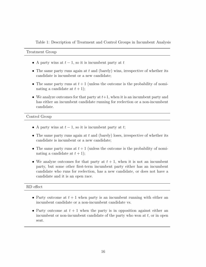
Table 1: Description of Treatment and Control Groups in Incumbent Analysis
Treatment Group
• A party wins at t− 1, so it is incumbent party at t
• The same party runs again at t and (barely) wins, irrespective of whether itscandidate is incumbent or a new candidate;
• The same party runs at t+ 1 (unless the outcome is the probability of nomi-nating a candidate at t+ 1);
• We analyze outcomes for that party at t+1, when it is an incumbent party andhas either an incumbent candidate running for reelection or a non-incumbentcandidate.
Control Group
• A party wins at t− 1, so it is incumbent party at t;
• The same party runs again at t and (barely) loses, irrespective of whether itscandidate is incumbent or a new candidate;
• The same party runs at t+ 1 (unless the outcome is the probability of nomi-nating a candidate at t+ 1);
• We analyze outcomes for that party at t + 1, when it is not an incumbentparty, but some other first-term incumbent party either has an incumbentcandidate who runs for reelection, has a new candidate, or does not have acandidate and it is an open race.
RD effect
• Party outcome at t + 1 when party is an incumbent running with either anincumbent candidate or a non-incumbent candidate vs.
• Party outcome at t + 1 when the party is in opposition against either anincumbent or non-incumbent candidate of the party who won at t, or in openseat.
16
t− 1, t and t+ 1. Because we are interested in an estimate of incumbency advantage for all
parties combined, we need to define a generic incumbent party. Naturally, in an incumbent
party analysis, at the point of realization of treatment assignment the party must have won
in the previous election – at t− 1 – to be considered an incumbent.
We present the results for the incumbent party analysis in two ways: pooling all election
years, and separately for each set of election triplets. In the latter analysis, five electoral
cycles (1996, 2000, 2004, 2008 and 2012) give us three election triplets: 1996/2000/2004,
2000/2004/2008 and 2004/2008/2012. We label each estimate according to the election at
which the treatment is assigned, i.e. the election at t (2000, 2004 and 2008).
The second type of analysis we perform focuses on the incumbency advantage of each
party. This individual party analysis is described in detail in Table 2. In this case, the RD
design is simpler: we just consider, for each party, whether it barely won or barely lost at t,
and analyze their outcomes at t+ 1.
Note that unlike for incumbent party analysis, where we require three adjacent elections
to define the RD effect, in this case, we require only two adjacent elections, and so our esti-
mates are pooled over four election pairs (1996/2000, 2000/2004, 2004/2008 and 2008/2012),
rather than over three election triplets, as in the first set of results.
Figure 1 shows the results of the incumbent party analysis on a pooled sample of all
election triplets and the three parties considered (PSDB, PMDB and DEM). We find a
strong negative incumbency advantage: an incumbent party barely winning an election is
around 21 percent less likely to win in the following election than if it barely lost. Based
on our data-driven optimal bandwidth choice procedure, we estimate this effect on the races
decided by a margin smaller than 16 percent of the vote. The estimated RD effect is highly
statistically significant.
The incumbency effect on the probability of victory is so large that we find a clear
incumbency disadvantage in terms of vote share as well. Bare winners on average lose around
3 percent of the vote compared to bare losers, and the robust confidence interval indicates a
17
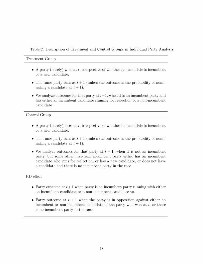
Table 2: Description of Treatment and Control Groups in Individual Party Analysis
Treatment Group
• A party (barely) wins at t, irrespective of whether its candidate is incumbentor a new candidate;
• The same party runs at t+ 1 (unless the outcome is the probability of nomi-nating a candidate at t+ 1);
• We analyze outcomes for that party at t+1, when it is an incumbent party andhas either an incumbent candidate running for reelection or a non-incumbentcandidate.
Control Group
• A party (barely) loses at t, irrespective of whether its candidate is incumbentor a new candidate;
• The same party runs at t+ 1 (unless the outcome is the probability of nomi-nating a candidate at t+ 1);
• We analyze outcomes for that party at t + 1, when it is not an incumbentparty, but some other first-term incumbent party either has an incumbentcandidate who runs for reelection, or has a new candidate, or does not havea candidate and there is no incumbent party in the race.
RD effect
• Party outcome at t+ 1 when party is an incumbent party running with eitheran incumbent candidate or a non-incumbent candidate vs.
• Party outcome at t + 1 when the party is in opposition against either anincumbent or non-incumbent candidate of the party who won at t, or thereis no incumbent party in the race.
18

Figure 1: Pooled Results for Incumbent Party
RD effectBandwidth
●
Candidate t+1−0.028 0.244
●
Victory t+1−0.213 0.153
●
Vote Share t+1−0.032 0.155
−0.4 −0.2 0.0 0.2 0.4
RD effects
Effect of Barely Winning on Several Outcomes
Note: Solid dots are RD effects (indicated in RD effects column) estimated via local linear regression and
mean-squared error optimal bandwidth (indicated in the Bandwidth column). Solid lines are 95% robust
confidence intervals developed by Calonico et al. (2013b) and implemented in Stata package rdrobust
(Calonico et al. 2013a).
19
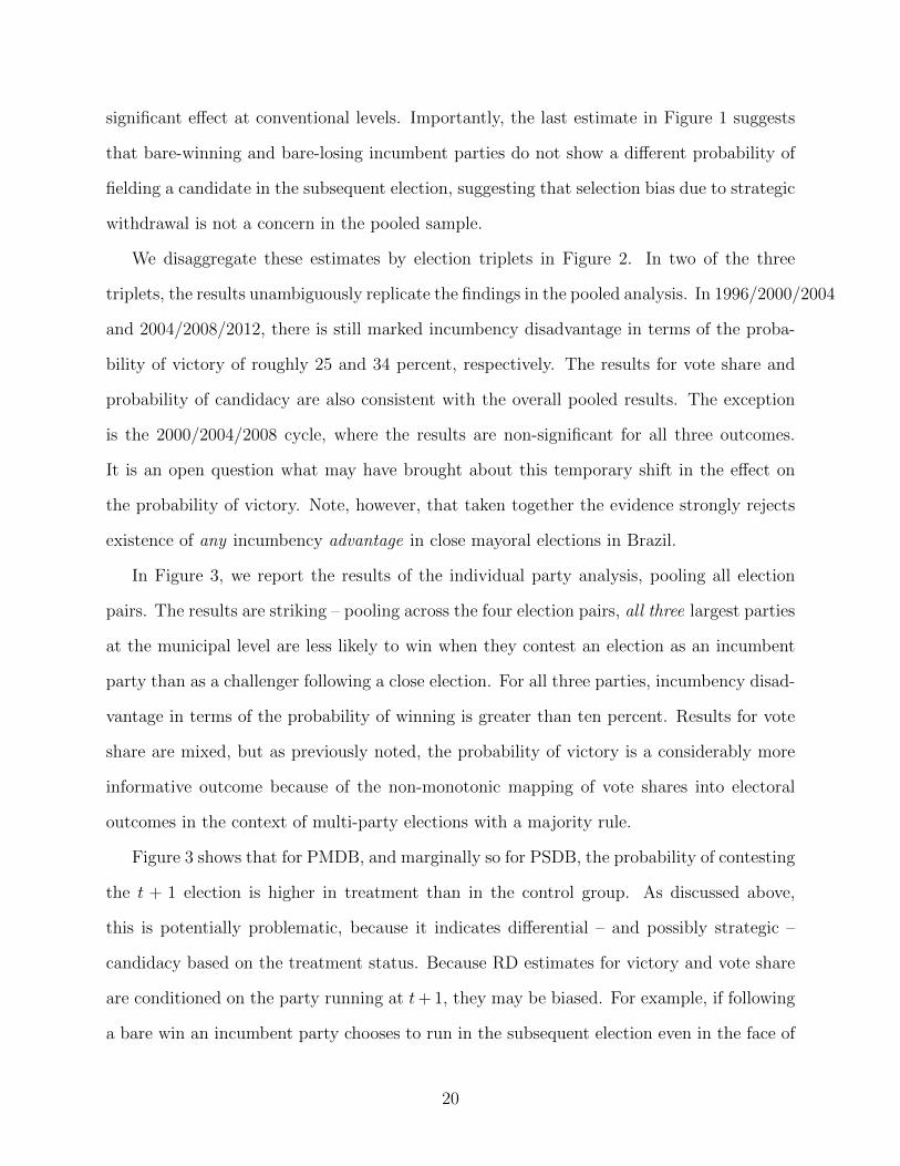
significant effect at conventional levels. Importantly, the last estimate in Figure 1 suggests
that bare-winning and bare-losing incumbent parties do not show a different probability of
fielding a candidate in the subsequent election, suggesting that selection bias due to strategic
withdrawal is not a concern in the pooled sample.
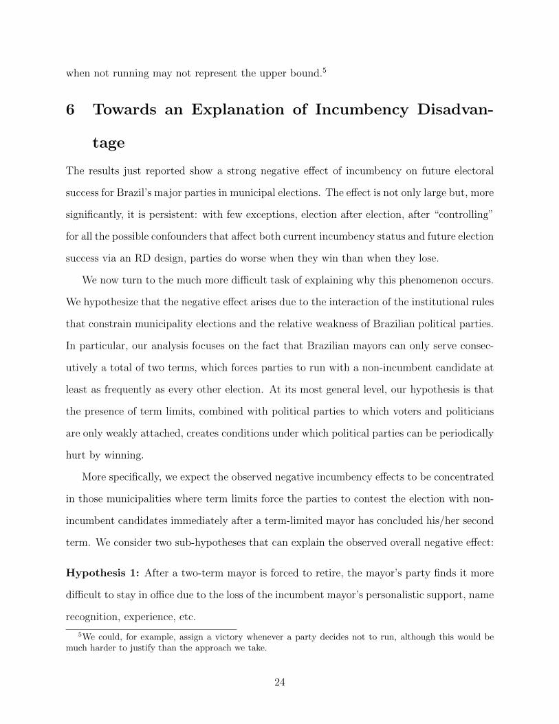
We disaggregate these estimates by election triplets in Figure 2. In two of the three
triplets, the results unambiguously replicate the findings in the pooled analysis. In 1996/2000/2004
and 2004/2008/2012, there is still marked incumbency disadvantage in terms of the proba-
bility of victory of roughly 25 and 34 percent, respectively. The results for vote share and
probability of candidacy are also consistent with the overall pooled results. The exception
is the 2000/2004/2008 cycle, where the results are non-significant for all three outcomes.
It is an open question what may have brought about this temporary shift in the effect on
the probability of victory. Note, however, that taken together the evidence strongly rejects
existence of any incumbency advantage in close mayoral elections in Brazil.
In Figure 3, we report the results of the individual party analysis, pooling all election
pairs. The results are striking – pooling across the four election pairs, all three largest parties
at the municipal level are less likely to win when they contest an election as an incumbent
party than as a challenger following a close election. For all three parties, incumbency disad-
vantage in terms of the probability of winning is greater than ten percent. Results for vote
share are mixed, but as previously noted, the probability of victory is a considerably more
informative outcome because of the non-monotonic mapping of vote shares into electoral
outcomes in the context of multi-party elections with a majority rule.
Figure 3 shows that for PMDB, and marginally so for PSDB, the probability of contesting
the t + 1 election is higher in treatment than in the control group. As discussed above,
this is potentially problematic, because it indicates differential – and possibly strategic –
candidacy based on the treatment status. Because RD estimates for victory and vote share
are conditioned on the party running at t+ 1, they may be biased. For example, if following
a bare win an incumbent party chooses to run in the subsequent election even in the face of
20

Figure 2: Disaggregated Results for Incumbent Party
RD effectBandwidth
●
Candidate t+1 2000−0.003 0.175
●
Candidate t+1 2004−0.025 0.143
●
Candidate t+1 2008−0.072 0.186
●
Victory t+1 2000−0.335 0.187
●
Victory t+1 2004−0.084 0.153
●
Victory t+1 2008−0.245 0.182
●
Vote Share t+1 2000−0.079 0.155
●
Vote Share t+1 20040.037 0.109
●
Vote Share t+1 2008−0.04 0.149
−0.6 −0.4 −0.2 0.0 0.2 0.4 0.6
RD effects
Effect of Barely Winning on Several Outcomes
Note: Solid dots are RD effects (indicated in RD effects column) estimated via local linear regression and
mean-squared error optimal bandwidth (indicated in the Bandwidth column). Solid lines are 95% robust
confidence intervals developed by Calonico et al. (2013b) and implemented in Stata package rdrobust
(Calonico et al. 2013a).
21

Figure 3: Pooled Results for PMDB, PSDB and DEM
RD effectBandwidth
●
Candidate t+1 PMDB0.037 0.173
●
Candidate t+1 PSDB0.064 0.213
●
Candidate t+1 DEM−0.014 0.151
●
Victory t+1 PMDB−0.191 0.146
●
Victory t+1 PSDB−0.112 0.195
●
Victory t+1 DEM−0.151 0.15
●
Vote Share t+1 PMDB−0.03 0.144
●
Vote Share t+1 PSDB0.009 0.161
●
Vote Share t+1 DEM−0.016 0.143
−0.6 −0.4 −0.2 0.0 0.2 0.4 0.6
RD effects
Effect of Barely Winning on Several Outcomes
Note: Solid dots are RD effects (indicated in RD effects column) estimated via local linear regression and
mean-squared error optimal bandwidth (indicated in the Bandwidth column). Solid lines are 95% robust
confidence intervals developed by Calonico et al. (2013b) and implemented in Stata package rdrobust
(Calonico et al. 2013a).
22

a weaker electoral prospect than if following a bare loss, the bias would be in the direction of
the results we find. This is because ceteris paribus, an incumbent party will have fared worse
than a challenger who strategically withdrew to avoid a poorer electoral return, dragging
the estimate of incumbency advantage down (or inflating the incumbency disadvantage).
To test the robustness of our results against such potential selection bias, we estimate
bounds on the RD effect on the probability of victory at t + 1. If not running indicates an
expectation of a poor result, than the worst-case scenario is to assume that the party not
running would never have won had it decided to contest. Using the notation from Section
3, this is equivalent to recoding the victory outcome variable as follows:
Yit,k ≡
1 if party runs at t+ 1 and wins,
0 if party runs t+1 and loses, or if party does not run at t+ 1.
(3)
In other words, where previously we omitted from the sample municipalities where a
party does not run at t+1 when estimating the RD effect on victory (or vote share), we now
assume that the party lost, despite not running. If not running implies attempting to avoid a
poor electoral outcome at t+1, and because results for PMDB and PSDB in Figure 3 suggest
that these parties were less likely to run when being a challenger at t + 1, assigning a loss
when not running represents an upper bound to our estimate of incumbency disadvantage.
This is because more challengers than incumbents will have been assigned a loss than when
conditioning on rerunning, boosting the estimated electoral performance of the incumbents.
If the RD estimate of the incumbency disadvantage is nevertheless still below zero and
significant, we can be confident under this set of assumptions on strategic retirement that it
is robust to the selection bias. This is indeed what we find. In Figures 4 and 5 we compare
the original Victory t+ 1 (conditional on the party running) to Upper Bound Victory t+ 1
(the recoded outcome as described above). Once we recode not running to losing, our point
estimates for victory are somewhat lower, but are substantively unaffected – we still find
incumbency disadvantage. Of course, under a different set of assumptions, assigning a loss
23
when not running may not represent the upper bound.5
6 Towards an Explanation of Incumbency Disadvan-
tage
The results just reported show a strong negative effect of incumbency on future electoral
success for Brazil’s major parties in municipal elections. The effect is not only large but, more
significantly, it is persistent: with few exceptions, election after election, after “controlling”
for all the possible confounders that affect both current incumbency status and future election
success via an RD design, parties do worse when they win than when they lose.
We now turn to the much more difficult task of explaining why this phenomenon occurs.
We hypothesize that the negative effect arises due to the interaction of the institutional rules
that constrain municipality elections and the relative weakness of Brazilian political parties.
In particular, our analysis focuses on the fact that Brazilian mayors can only serve consec-
utively a total of two terms, which forces parties to run with a non-incumbent candidate at
least as frequently as every other election. At its most general level, our hypothesis is that
the presence of term limits, combined with political parties to which voters and politicians
are only weakly attached, creates conditions under which political parties can be periodically
hurt by winning.
More specifically, we expect the observed negative incumbency effects to be concentrated
in those municipalities where term limits force the parties to contest the election with non-
incumbent candidates immediately after a term-limited mayor has concluded his/her second
term. We consider two sub-hypotheses that can explain the observed overall negative effect:
Hypothesis 1: After a two-term mayor is forced to retire, the mayor’s party finds it more
difficult to stay in office due to the loss of the incumbent mayor’s personalistic support, name
recognition, experience, etc.
5We could, for example, assign a victory whenever a party decides not to run, although this would bemuch harder to justify than the approach we take.
24
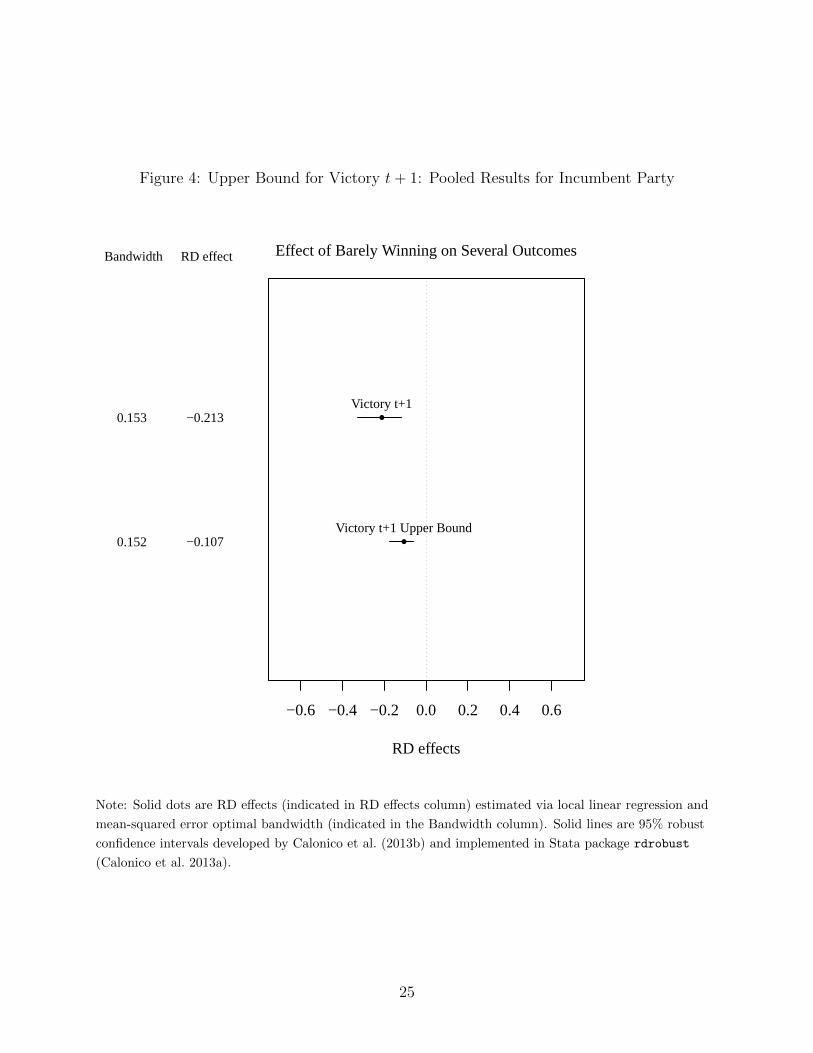
Figure 4: Upper Bound for Victory t+ 1: Pooled Results for Incumbent Party
RD effectBandwidth
●
Victory t+1 Upper Bound−0.107 0.152
●
Victory t+1−0.213 0.153
−0.6 −0.4 −0.2 0.0 0.2 0.4 0.6
RD effects
Effect of Barely Winning on Several Outcomes
Note: Solid dots are RD effects (indicated in RD effects column) estimated via local linear regression and
mean-squared error optimal bandwidth (indicated in the Bandwidth column). Solid lines are 95% robust
confidence intervals developed by Calonico et al. (2013b) and implemented in Stata package rdrobust
(Calonico et al. 2013a).
25
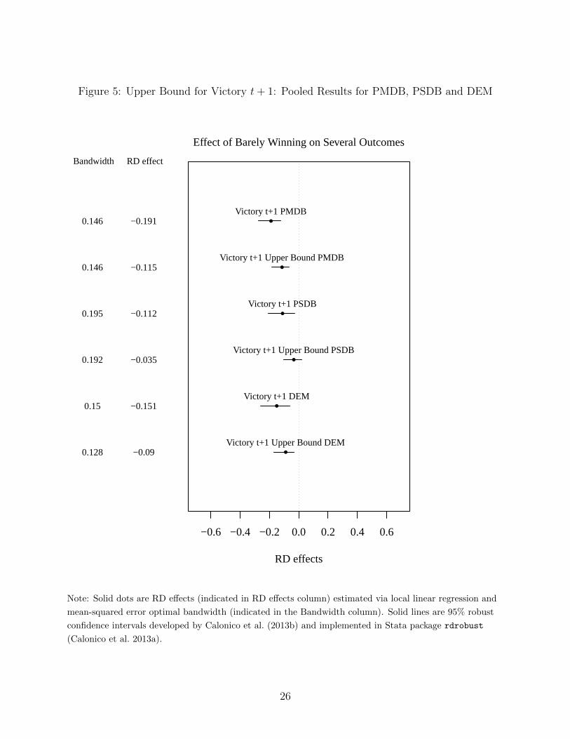
Figure 5: Upper Bound for Victory t+ 1: Pooled Results for PMDB, PSDB and DEM
RD effectBandwidth
●
Victory t+1 Upper Bound DEM−0.09 0.128
●
Victory t+1 DEM−0.151 0.15
●
Victory t+1 Upper Bound PSDB−0.035 0.192
●
Victory t+1 PSDB−0.112 0.195
●
Victory t+1 Upper Bound PMDB−0.115 0.146
●
Victory t+1 PMDB−0.191 0.146
−0.6 −0.4 −0.2 0.0 0.2 0.4 0.6
RD effects
Effect of Barely Winning on Several Outcomes
Note: Solid dots are RD effects (indicated in RD effects column) estimated via local linear regression and
mean-squared error optimal bandwidth (indicated in the Bandwidth column). Solid lines are 95% robust
confidence intervals developed by Calonico et al. (2013b) and implemented in Stata package rdrobust
(Calonico et al. 2013a).
26
Hypothesis 2: After a two-term mayor is forced to retire, the mayor’s party finds it more
difficult to stay in office due to the mayor’s shirking behavior in his last term, for which
voters punish the mayor’s party.
Basic facts about the Brazilian party system can support both hypotheses. Brazilian parties
have low levels of institutionalization and, particularly in local elections, political networks
are highly personalistic. In this context, the forced retirement of mayors who have proved
successful enough to be reelected may result in losses for his party. On the other hand, there
is also evidence that corruption is considerably higher and effort lower in municipalities
where mayors cannot run for reelection (see Ferraz and Finan 2011), which indicates that
mayors tend to engage in shirking in the absence of reelection incentives.6
Unfortunately, it is difficult to explore these hypothesis with a strong quasi-experimental
design. In the RD design that we used above to characterize the overall party incumbency
effects, very close races allow us to proceed “as if” victory at election t had been randomly
assigned. But there is no similar as-if randomization for mayors’ decisions to run for re-
election, which is at the center of both of our hypotheses. Although we cannot solve this
inferential issue, we analyze two subsamples of our dataset where, based on our hypotheses,
the effects are predicted to be different. This tentative analysis can show that our hypotheses
are consistent with the observed results, but it cannot prove that they are correct.
We now describe our conditional analysis for the incumbent party analysis. Our condi-
tional analysis divides the sample in two mutually exclusive subsets. The Incumbent Sample
is composed of all municipalities where the candidate who got elected at t − 1 for a given
party runs for reelection at t under the same party.7 The Open Seats Sample is composed
of all municipalities where the candidate who got elected at t− 1 for a given party does not
run for reelection at t. Note that the incumbent candidates’ decision to run for reelection,
6This has been shown in other contexts as well; see for example Alt et al. (2011); Besley and Case (1995).7We exclude cases where the candidate who got elected at t − 1 for a given party runs for reelection at
t under a different party. In future versions, we plan to leverage these party switches to provide furtherevidence about our hypothesized mechanisms.
27
although clearly endogenous, is made before election t is held. Thus, we are legitimately
subsetting our data based on a pre-treatment variable.
We describe the Incumbent Sample in Table 3, and the Open Seat Sample in Table 4.
For our purposes, the most important difference between the two samples is whether the
party is running immediately after a lame-duck mayor has retired. The Open Seat sample
contains a combination of incumbent candidates and non-incumbent candidates in both the
treated and control group. In contrast, in the Incumbent Sample, the same combination
of incumbent and non-incumbent candidates exists in the control group, but the treatment
group is composed exclusively of non-incumbent candidates who are running immediately
after the party’s previous incumbents have finished their second and last term and are
therefore prohibited from running at t + 1. Under Hypotheses 1 and 2, we expect to see a
concentration of the negative effects of incumbency in the Incumbent Sample rather than in
the Open Seat Sample.
Figure 6 presents a comparison of the incumbency effects for the incumbent party, pooling
across all elections. The results strongly support our prediction. Neither effect is significant
at conventional levels in the Open Seat Sample: the effect on Vote Share t+ 1 is extremely
close to zero (−0.006), and the confidence interval is tight; the point estimate for Victory
t + 1 is negative and large (−0.101), but it is not significant at 5% level. Finally, the
incumbent party does not seem to be more likely to contest the election at t+1. In contrast,
in the Incumbent Sample, the effect on Vote Share t + 1 is ten times larger (−0.06) and
highly statistically significant, and the effect on Victory t+ 1 triples to −0.327 and becomes
strongly significant. In addition, in this sample, the incumbent party is significantly less
likely to contest the t+ 1 election after a bare victory at t.
Figures 7, 8 and 9 present analogous figures, disaggregating the incumbent party analysis
for each election. Again, the results support our prediction in each of the three election
triplets. In all cases, the point estimate for Victory t+ 1 is smaller in the Incumbent Sample
than in the Open Seat Sample and, with the exception of 2000 (1996/2000/2004 triplet), the
28
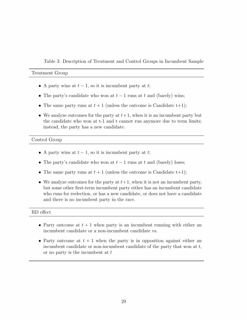
Table 3: Description of Treatment and Control Groups in Incumbent Sample
Treatment Group
• A party wins at t− 1, so it is incumbent party at t;
• The party’s candidate who won at t− 1 runs at t and (barely) wins;
• The same party runs at t+ 1 (unless the outcome is Candidate t+1);
• We analyze outcomes for the party at t+1, when it is an incumbent party butthe candidate who won at t-1 and t cannot run anymore due to term limits;instead, the party has a new candidate.
Control Group
• A party wins at t− 1, so it is incumbent party at t;
• The party’s candidate who won at t− 1 runs at t and (barely) loses;
• The same party runs at t+ 1 (unless the outcome is Candidate t+1);
• We analyze outcomes for the party at t+1, when it is not an incumbent party,but some other first-term incumbent party either has an incumbent candidatewho runs for reelection, or has a new candidate, or does not have a candidateand there is no incumbent party in the race.
RD effect
• Party outcome at t + 1 when party is an incumbent running with either anincumbent candidate or a non-incumbent candidate vs.
• Party outcome at t + 1 when the party is in opposition against either anincumbent candidate or non-incumbent candidate of the party that won at t,or no party is the incumbent at t
29

Table 4: Description of Treatment and Control Groups in Open Seat Sample
Treatment Group
• A party wins at t− 1, so it is incumbent party at t;
• The party’s candidate who won at t− 1 does not run at t, but the party runswith another candidate and (barely) wins;
• The same party runs at t+ 1 (unless the outcome is Candidate t+1);
• We analyze outcomes for the party at t + 1, when it is an incumbent partyand it either runs with an incumbent candidate who seeks reelection or witha new non-incumbent candidate or it does not run and there is no incumbentparty in the race.
Control Group
• A party wins at t− 1, so it is incumbent party at t;
• The party’s candidate who won at t− 1 does not run at t, but the party runswith another candidate and (barely) loses;
• The same party runs at t+ 1 (unless the outcome is Candidate t+1);
• We analyze outcomes for the party at t+1, when it is not an incumbent party,but some other first-term incumbent party either has an incumbent candidatewho runs for reelection, or has a new candidate, or does not have a candidateand there is no incumbent party in the race.
RD effect
• Party outcome at t + 1 when party is an incumbent running with either anincumbent candidate or a non-incumbent candidate vs.
• Party outcome at t + 1 when the party is in opposition against either anincumbent candidate or non-incumbent candidate of the party that won at t,or in seat where no party is the incumbent.
30

Figure 6: Incumbent Sample versus Open Seat Sample: Incumbent Party Pooling All Elec-tions
RD effectBandwidth
●
Candidate t+1 Incumbent seats−0.088 0.25
●
Candidate t+1 Open seats0.044 0.197
●
Victory t+1 Incumbent seats−0.327 0.147
●
Victory t+1 Open seats−0.101 0.21
●
Vote Share t+1 Incumbent seats−0.06 0.15
●
Vote Share t+1 Open seats−0.006 0.152
−0.6 −0.4 −0.2 0.0 0.2 0.4 0.6
RD effects
Effect of Barely Winning on Several Outcomes Incumbent Party
Note: Solid dots are RD effects (indicated in RD effects column) estimated via local linear regression and
mean-squared error optimal bandwidth (indicated in the Bandwidth column). Solid lines are 95% robust
confidence intervals developed by Calonico et al. (2013b) and implemented in Stata package rdrobust
(Calonico et al. 2013a).
31

effect on Victory t+ 1 is insignificant in the Open Seat Sample and highly significant in the
Incumbent Sample.
32

Figure 7: Incumbent Sample versus Open Seat Sample: Incumbent Party in 2000
RD effectBandwidth
●
Candidate t+1 Open seats0.015 0.267
●
Candidate t+1 Incumbent seats−0.003 0.151
●
Victory t+1 Open seats−0.289 0.195
●
Victory t+1 Incumbent seats−0.365 0.132
●
Vote Share t+1 Open seats−0.084 0.185
●
Vote Share t+1 Incumbent seats−0.077 0.159
−1.0 −0.5 0.0 0.5 1.0
RD effects
Effect of Barely Winning on Several Outcomes
Note: Solid dots are RD effects (indicated in RD effects column) estimated via local linear regression and
mean-squared error optimal bandwidth (indicated in the Bandwidth column). Solid lines are 95% robust
confidence intervals developed by Calonico et al. (2013b) and implemented in Stata package rdrobust
(Calonico et al. 2013a). 33

Figure 8: Incumbent Sample versus Open Seat Sample: Incumbent Party in 2004
RD effectBandwidth
●
Candidate t+1 Open seats0.05 0.187
●
Candidate t+1 Incumbent seats−0.104 0.144
●
Victory t+1 Open seats−0.006 0.151
●
Victory t+1 Incumbent seats−0.242 0.16
●
Vote Share t+1 Open seats0.046 0.127
●
Vote Share t+1 Incumbent seats0.01 0.107
−1.0 −0.5 0.0 0.5 1.0
RD effects
Effect of Barely Winning on Several Outcomes
Note: Solid dots are RD effects (indicated in RD effects column) estimated via local linear regression and
mean-squared error optimal bandwidth (indicated in the Bandwidth column). Solid lines are 95% robust
confidence intervals developed by Calonico et al. (2013b) and implemented in Stata package rdrobust
(Calonico et al. 2013a).
34
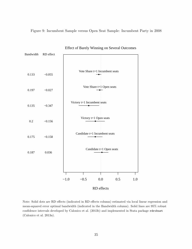
Figure 9: Incumbent Sample versus Open Seat Sample: Incumbent Party in 2008
RD effectBandwidth
●
Candidate t+1 Open seats0.036 0.187
●
Candidate t+1 Incumbent seats−0.158 0.175
●
Victory t+1 Open seats−0.156 0.2
●
Victory t+1 Incumbent seats−0.347 0.135
●
Vote Share t+1 Open seats−0.027 0.197
●
Vote Share t+1 Incumbent seats−0.055 0.133
−1.0 −0.5 0.0 0.5 1.0
RD effects
Effect of Barely Winning on Several Outcomes
Note: Solid dots are RD effects (indicated in RD effects column) estimated via local linear regression and
mean-squared error optimal bandwidth (indicated in the Bandwidth column). Solid lines are 95% robust
confidence intervals developed by Calonico et al. (2013b) and implemented in Stata package rdrobust
(Calonico et al. 2013a).
35

7 Conclusion
Using a regression discontinuity design to analyze Brazil’s municipal mayor elections, we
found strong negative effects of becoming the incumbent party on the probability of winning
in the following election. The results are negative for the three parties which control over
seventy percent of Brazilian municipalities and are consistent with the negative and non-
positive effects found by Linden (2004), Miguel and Zahidi (2004) and Uppal (2009) in
developing countries, but they are in sharp contrast to the large and positive effects typically
found in the U.S.
The finding of these large negative party incumbency effects for an executive office de-
serves further analysis and explanation. As explained in Section 2, Brazilian mayors enjoy
substantial autonomy and access to a large number of local resources, and thus they have
the ability of targeting resources to constituents. Therefore, the fact that the mayor’s party
is systematically punished cannot be easily explained by an inability of mayors to respond
to the desires of her constituents.
In Section 6 we advanced a tentative explanation that concentrates on the interaction of
the weakness of the Brazilian political parties, the short temporal horizon of mayors and the
general characteristics of the careers of Brazilian politicians. Mayors serve a four-year period,
and can only be consecutively elected for two terms. We hypothesized that the negative effect
would arise from those municipalities where parties contest the election after the mayor was
term-limited. We developed an indirect test of this hypothesis, which predicts different RD
effects for the two subsamples that arise by conditioning on whether the candidate who won
at t − 1 is a candidate at t. Importantly, this is a pre-treatment variable, and conditioning
on it preserves the internal validity of the comparison between treatment and control groups
within each subset. Consistent with our prediction, the effects in our Incumbent Sample,
where incumbent candidates run at t, are negative, large and significant, while the effects in
our Open Seat Sample, where no incumbent candidates run at t, are not distinguishable from
36

zero. Future versions of this manuscript will explore this promising result in more detail, in
order to develop a more comprehensive explanation of the negative incumbency effects that
allows us to further our understanding of the Brazilian party system.
37

References
Abrucio, F. L. (1998). Os Baroes da Federacao: O Poder dos Governadores no Brasil Pos-Autoritario. Sao Paulo: Universidade de Sao Paulo.
Aidt, T., M. A. Golden, and D. Tiwari (2011, September). Incumbents and criminals in theindian national legislature. Manuscript.
Alford, J. R. and D. W. Brady (1989). Personal and partisan advantage in us congressionalelections. In L. C. Dodd and B. I. Oppenheimer (Eds.), Congress Reconsidered 4th edition.Washington, D.C.: CQ Press.
Alt, J., E. B. de Mesquita, and S. Rose (2011). Disentangling accountability and competencein elections: Evidence from us term limits. Journal of Politics 73 (1), 171–186.
Ames, B. (2001a). The Deadlock of Democracy in Brazil. Ann Arbor: University of MichiganPress.
Ames, B. (2001b). Party discipline in brazil’s chamber of deputies. In S. Morgenstern andB. Nacif (Eds.), Legislative Politics in Latin America. New York: Cambridge UniversityPress.
Ansolabehere, S., D. W. Brady, and M. P. Fiorina (1988). The vanishing marginals andelectoral responsiveness. British Journal of Political Science 22 (1), 21–38.
Ansolabehere, S. and J. Snyder (2002). The incumbency advantage in u.s. elections: Ananalysis of state and federal offices, 1942-2000. Election Law Journal 1 (3), 315–338.
Ansolabehere, S., J. M. Snyder, and C. Stewart (2000). Old voters, new voters, and the per-sonal vote: Using redistricting to measure the incumbency advantage. American Journalof Political Science 44 (1), 17–34.
Besley, T. and A. Case (1995). Does electoral accountability affect economic policy choices?evidence from gubernatorial term limits. The Quarterly Journal of Economics 110 (3),769–798.
Birch, S. (2003). Electoral Systems and Political Transformation in Post-Communist Europe.New York, NY: Palgrave Macmillan.
Calonico, S., M. D. Cattaneo, and R. Titiunik (2013a). Robust data-driven inference in theregression-discontinuity design. Manuscript.
Calonico, S., M. D. Cattaneo, and R. Titiunik (2013b). Robust nonparametric confidenceintervals for regression-discontinuity designs. Manuscript.
Carey, J. M. and G. Y. Reinhardt (2001). Coalition brokers or breakers? brazilian governorsand legislative voting. Working Paper, Washington University, St. Louis.
38

Collier, R. B. and D. Collier (2002). Shaping the Political Arena: Critical Junctures, theLabor Movement, and Regime Dynamics in Latin America. Indiana: University of NotreDame Press.
Cook, T. D. (2008). ”waiting for life to arrive”: a history of the regression-discontinuitydesign in psychology, statistics and economics. Journal of Econometrics 142 (2), 636–654.
Costa, V. L. C. (1998). Descentralizacao de educacao no brasil: As reformas recentes noensido fundamental. Paper presented at the Latin American Studies Meeting, Chicago.
Cox, G. W. and J. N. Katz (1996). Why did the incumbency advantage in u.s. house electionsgrow. American Journal of Political Science 40 (2), 478–497.
Cox, G. W. and J. N. Katz (2002). Elbridge Gerry’s Salamander: The Electoral Consequencesof the Reapportionment Revolution. New York: Cambridge University Press.
Cox, G. W. and S. Morgenstern (1993). The increasing advantage of incumbency in the u.s.states. Legislative Studies Quarterly 18 (4), 495–514.
Desposato, S. W. (2006). Parties for rent? ambition, ideology, and party switching in brazil’schamber of deputies. American Journal of Political Science 50 (1), 62–80.
Eggers, A. C., O. Folke, A. Fowler, J. Hainmueller, A. B. Hall, and J. M. Snyder (2013, June).On the validity of the regression discontinuity design for estimating electoral effects: Newevidence from over 40,000 close races. Manuscript.
Erikson, R. and R. Titiunik (2013). Using regression discontinuity to uncover the personalincumbency advantage.
Erikson, R. S. (1971). The advantage of incumbency in congressional elections. Polity 3 (3),395–405.
Erikson, R. S. (1972). Malapportionment, gerrymandering, and party fortunes in congres-sional elections. American Political Science Review 65 (4), 1234–1245.
Ferejohn, J. A. (1977). On the decline of competition in congressional elections. AmericanPolitical Science Review 71 (1), 166–176.
Ferraz, C. and F. Finan (2011). Electoral accountability and corruption: Evidence from theaudits of local governments. American Economic Review 101, 1274–1311.
Figueiredo, A. C. and F. Limongi (2000). Presidential power, legislative organization andparty behavior in brazil. Comparative Politics 32 (2), 151–170.
Fiorina, M. P. (1977). The case of the vanishing marginals: The bureaucracy did it. AmericanPolitical Science Review 71 (1), 177–181.
Fisman, R., F. Schulz, and V. Vig (2012, May). Private returns to public office. NBERWorking Paper 18095.
39

Gelman, A. and G. King (1990). Estimating incumbency advantage without bias. AmericanJournal of Political Science 34 (4), 1142–1164.
Hahn, J., P. Todd, and W. van der Klaauw (2001). Identification and estimation of treatmenteffects with a regression-discontinuity design. Econometrica 69, 201–209.
IBGE (2001). Pesquisa de Informacoes Basicas Municipais, Gestao Publica 2001. Rio deJaneiro: Instituto Brasileiro de Geografia e Estatistica.
IBGE (2002). Pesquisa de Informacoes Basicas Municipais, Gestao Publica 2002. Rio deJaneiro: Instituto Brasileiro de Geografia e Estatistica.
IBGE (2004). Produto Interno Bruto dos Municıpios. Rio de Janeiro: Serie RelatoriosMetodologicos, Vol. 29. Instituto Brasileiro de Geografia e Estatistica.
Imbens, G. and T. Lemieux (2008). Regression discontinuity designs: A guide to practice.Journal of Econometrics 142 (2), 615–635.
Imbens, G. W. and K. Kalyanaraman (2012). Optimal bandwidth choice for the regressiondiscontinuity estimator. forthcoming in Review of Economic Studies .
Jacobson, G. C. (1987). The marginals never vanished: Incumbency and competition inelections to the u.s. house of representatives. American Journal of Political Science 31 (1),126–141.
Kinzo, M. D. G. (2003). Parties and elections: Brazil’s democratic experience since 1985. InM. D. G. Kinzo and J. Dunkerley (Eds.), Brazil Since 1985: Economy, Polity and Society.University of London: Institute of Latin American Studies.
Krehbiel, K. and J. R. Wright (1983). The incumbency effect in congressional elections: Atest of two explanations. American Journal of Political Science 27 (1), 140–157.
Lee, D. S. (2008). Randomized experiments from non-random selection in u.s. house elections.Journal of Econometrics 142 (2), 675–697.
Lee, D. S. and T. Lemieux (2010). Regression discontinuity designs in economics. Journalof Economic Literature 48 (2), 281–355.
Levitt, S. D. and C. D. Wolfram (1997). Decomposing the sources of incumbency advantagein the u.s. house. Legislative Studies Quarterly 22 (1), 45–60.
Linden, L. (2004). Are incumbents really advantaged? the preference for non-incumbents inindian national elections. Working Paper.
Mainwaring, S. (1991). Politicians, parties, and electoral systems: Brazil in comparativeperspective. Comparative Politics 24 (1), 21–43.
Mainwaring, S. (1993). Brazilian party underdevelopment in comparative perspective. Po-litical Science Quarterly 107 (4), 677–707.
40
Mainwaring, S. (1999). Rethinking Party Systems in the Third Wave of Democratization:The Case of Brazil. Stanford: Stanford University Press.
Miguel, E. and F. Zahidi (2004). Do politicians reward their supporters? public spendingand incumbency advantage. Working Paper.
Montero, A. P. (2005). Brazilian Politics. Massachusetts: Polity Press.
Nickson, R. A. (1995). Local Government in Latin America. Boulder: Lynne Rienner.
Pop-Eleches, G. (2010). Throwing out the bums: Protest voting and unorthodox partiesafter communism. World Politics 62, 221–260.
Roberts, A. (2008). Hyperaccountability: Economic voting in central and eastern europe.Electoral Studies 27, 533–546.
Samuels, D. J. (1998). Political ambition in brazil, 1945–95: Theory and evidence. WorkingPaper, University of Minnesota.
Samuels, D. J. (1999a). Ambition, Federalism, and Legislative Politics in Brazil. Cambridge,UK: Cambridge University Press.
Samuels, D. J. (1999b). Incentives to cultivate a party vote in candidate-centric electoralsystems: Evidence from brazil. Comparative Political Studies 32 (4), 487–518.
Samuels, D. J. (2000a). Concurrent elections, discordant results. presidentialism, federalism,and governance in brazil. Comparative Politics 33 (1), 1–20.
Samuels, D. J. (2000b). The political logic of decentralization in brazil. In P. Kingstoneand T. J. Power (Eds.), Democratic Brazil. Actors Institutions and Processes. Pittsburgh,Pennsylvania: University of Pittsburgh Press.
Samuels, D. J. (2002). Ambassadors of the States: Political Ambition, Federalism, andCongressional Politics in Brazil. Cambridge, MA: Cambridge University Press.
Samuels, D. J. (2004). The political logic of decentralization in brazil. In A. P. Monteroand D. J. Samuels (Eds.), Decentralization and Democracy in Latin America. Indiana:University of Notre Dame Press.
Samuels, D. J. and F. L. Abrucio (2000). Federalism and democratic transitions: The ”new”politics of the governors in brazil. Publius 30 (2), 43–61.
Sekhon, J. S. and R. Titiunik (2012). When natural experiments are neither natural norexperiments. American Political Science Review 106 (01), 35–57.
Thistlethwaite, D. and D. Campbell (1960). Regression-discontinuity analysis: An alterna-tive to the ex post facto experiment. Journal of Educational Psychology 51, 309–317.
Uppal, Y. (2009). The disadvantaged incumbents: estimating incumbency effects in indianstate legislatures. Public Choice 138 (1-2), 9–27.
41