Independent and A¢ liated Analysts:

Disciplining and Herding�

Hao Xue

Carnegie Mellon University

December 20, 2012

Abstract

The paper investigates strategic interactions between an independent analyst and

an a¢ liated analyst when the analysts�information acquisition and the timing of their

recommendations are endogenous. Compared to the independent analyst, the a¢ liated

analyst has superior information but faces a con�ict of interest. I show that the indepen-

dent analyst�s recommendation, albeit endogenously less informative than the a¢ liated

analyst�s, disciplines the a¢ liated analyst�s biased forecasting behavior. Meanwhile, the

independent analyst sometimes herds with the a¢ liated analyst in order to improve fore-

cast accuracy. Contrary to conventional wisdom, I show that herding with the a¢ liated

analyst may actually motivate the independent analyst to acquire more information up-

front, reinforce his ability to discipline the a¢ liated analyst, and bene�t investors.

�I am greatly indebted to my dissertation committee chair Jonathan Glover for his guidance and help. I amalso grateful to Pierre Liang, Carlos Corona, and Zhaoyang Gu for their invaluable comments and suggestions.I thank Anil Arya, Anne Beyer, Pingyang Gao, Isa Hafalir, Jing Li, Xiaojing Meng, John O�Brien, Jack Stecher,and workshop participants at Carnegie Mellon University. The paper is also bene�ted from discussions withmy fellow Ph.D. students Qihang Lin and Ronghuo Zheng and my wife Hui Wang. All errors are my own.

1

1 Introduction

This paper investigates strategic interactions between an independent analyst and an a¢ liated

analyst when the analysts�information acquisition and the timing of their recommendations

are endogenous. In the paper, I di¤erentiate a¢ liated analysts from independent analysts

by two features: (a) the a¢ liated analyst faces a con�ict of interest and (b) he has superior

information compared to the independent analyst.

These two features have been widely noted by regulatory bodies, practitioners, and re-

searchers. For example, the Global Analyst Research Settlement (Global Settlement) between

the United States�regulators and the nation�s top investment �rms directly addresses con�icts

of interest between research and investment banking businesses. An example of superior in-

formation a¢ liated analysts receive is con�dential, non-public information they obtain in the

due diligence process as an underwriter in an Initial Public O¤ering (IPO). The inappropriate

release of such con�dential information in a restricted period prior to Facebook�s IPO was the

focus of the Commonwealth of Massachusetts�case against Citigroup.1 Empirically, Lin and

McNichols (1998), Irvine (2004), and Mola and Guidolin (2009) document evidence suggesting

that a¢ liated analysts face con�icts of interest,2 while Jacob et al. (2008) and Chen and Mar-

tin (2011) document evidence suggesting that analysts receive superior information because of

their a¢ liations with the company.

On one hand, researchers argue that independent analysts�incentives are more aligned with

investors and �nd the existence of independent analysts disciplines a¢ liated analysts�biased

forecasting behavior (e.g., Gu and Xue, 2008). Consistent with the disciplining argument,

the Global Settlement requires investment banks to acquire and distribute three independent

research reports along with their own reports for every company they cover. On the other

hand, since independent analysts�information is inferior, it is reasonable to suspect they have

incentives to herd with a¢ liated analysts, given the well-documented herding behavior among

1http://www.sec.state.ma.us/sct/current/sctciti/Citi_Consent.pdf2There is mixed evidence on whether a¢ liated analysts purposely bias their forecasts (see Beyer et al.,

2010 for a comprehensive review of the mixed evidences). I will return to this later and argue that my modelreconciles some of the mixed evidence.

2

�nancial analysts (e.g., Welch, 2000; Hirshleifer and Teoh, 2003).

If independent analysts herd with a¢ liated analysts, to what extent is their disciplining

role compromised? Casual intuition suggests that herding would jeopardize the ability to

discipline, which is consistent with the prevailing view in academic research that analysts�

herding behavior discourages information production and is undesirable from the investor�s

perspective. In the Abstract of Herding Behavior among Financial Analysts: A Literature

Review, Van Campenhout and Verhestraeten (2010) write:

Analysts�forecasts are often used as an information source by other investors, and

therefore deviations from optimal forecasts are troublesome. Herding, which refers

to imitation behavior as a consequence of individual considerations, can lead to

such suboptimal forecasts and is therefore widely studied.

Contrary to conventional wisdom, this paper shows that the independent analyst�s disci-

plining role and herding behavior may reinforce each other. I show that if the independent

analyst�s informational disadvantage is large, herding with the a¢ liated analyst actually moti-

vates the independent analyst to acquire more information upfront, reinforces his disciplining

role, and ultimately bene�ts the investor.

The model has three players: an a¢ liated analyst, an independent analyst, and an investor.

Each analyst acquires a private signal about an underlying, risky asset (the �rm) and publicly

issues a stock recommendation at a time that is strategically chosen. When choosing the timing

of their recommendations, both analysts face a trade-o¤ between the accuracy and timeliness

of their recommendations.3 Compared to the independent analyst, the a¢ liated analyst is

assumed to face a con�ict of interest but has superior information. To model the a¢ liated

analyst�s con�ict of interest, I assume he receives an additional reward (independent of the

reward for timeliness and accuracy) if the investor is convinced to buy the stock. To model

the independent analyst�s informational disadvantage, I assume the signal he endogenously

acquires is less precise than the a¢ liated analyst�s signal due to exogenous higher information

3See Schipper (1991) and Gul and Lundholm (1995) on the tradeo¤ between accuracy and timeliness ofrecommendations.

3

acquisition costs. The precision of the analysts�information is interpreted as a �rm-wide choice

(e.g., hiring a star analyst or devoting more resources to a speci�c industry) and is assumed

to be publicly observed.

Due to his con�ict of interest, the a¢ liated analyst has an incentive to over-report a bad

signal in order to induce the investor to buy the stock. The model shows that the independent

analyst disciplines the a¢ liated analyst�s biased forecasting behavior in equilibrium. Intu-

itively, since the independent analyst�s recommendation provides information to the investor,

the extent the a¢ liated analyst can misreport his signal without being ignored by the investor

is bounded by the quality of the independent analyst�s recommendation.

The independent analyst�s herding behavior also arises in equilibrium. Since the analysts�

recommendations can be either favorable or unfavorable, the only reason for the independent

analyst to delay his recommendation is to herd with the a¢ liated analyst. In equilibrium,

the a¢ liated analyst�s unfavorable recommendation is more informative than his favorable

recommendation, so the independent analyst�s expected bene�t from waiting is higher if his

private signal is good. The endogenous bene�t of waiting, together with an exogenous cost of

waiting, leads to a conditional herding equilibrium under which the independent analyst reports

a bad signal immediately but waits and herds with the a¢ liated analyst upon observing a good

signal.

Surprisingly, conditional herding causes the independent analyst to acquire more informa-

tion and play a greater disciplining role than if he were prohibited from herding. The reason

is that herding introduces an indirect bene�t to information acquisition. By acquiring better

information and reporting a bad signal right away, the independent analyst motivates the af-

�liated analyst to truthfully reveal a bad signal more often �this is the disciplining role. The

a¢ liated analyst�s more accurate reporting means that the independent analyst who receives a

good signal too will be more accurate, since he herds with the a¢ liated analyst. This indirect

bene�t of information acquisition derived from herding motivates the independent analyst to

acquire better information upfront. That is, there is an induced complementarity between the

independent analyst�s ex-post herding and ex-ante information acquisition.

4

Empirical Implications

First, the model predicts a positive association between independent analysts�degree of

herding4 with a¢ liated analysts and the informativeness of a¢ liated analysts�recommendations

for �rms with high information acquisition costs. The predicted association is negative for �rms

with low information acquisition costs.

Second, the model predicts that the dispersion between a¢ liated and independent ana-

lysts� recommendations decreases over time. Moreover, the decrease of dispersion is driven

by independent analysts�recommendations converging to a¢ liated analysts�recommendations

but not vice versa. The prediction of a shrinking dispersion is consistent with O�Brien et al.

(2005) and Bradshaw et al. (2006) who found that a¢ liated analysts�recommendations are

more optimistic than independent analysts�only in the �rst several months surrounding public

o¤erings, while there is no di¤erence afterwards.5

Third, the model predicts that a¢ liated analysts�recommendations are both more opti-

mistic and more informative than independent analysts�. Evidence consistent with the coex-

istence of a¢ liated analysts�optimism and superiority is documented by Dugar and Nathan

(1995) and Lin and McNichols (1998).6

Regulatory Implications

First, the model shows a¢ liated analysts can be disciplined by independent analysts even

when the latter�s recommendations are less informative and involve herding behavior. The

result that the independent analyst herding with the a¢ liated analyst may actually bene�t the

investor is relevant in the light of the Jumpstart Our Business Startups Act (JOBS Act). The

JOBS Act permits a¢ liated analysts to publish research reports with respect to an emerging

growth company any time after its IPO.7 The paper suggests that making it possible for inde-

pendent analysts to herd with a¢ liated analysts right after the IPO may increase independent

4Zitzewitz (2001) proposes a methodology for estimating the degree of herding.5O�Brien et al. (2005) write �we choose public o¤erings as a starting point because the �nancing event

allows us to distinguish a¢ liated from una¢ liated analysts.�6Gu and Wu (2003) argue that if analysts� objective is to minimize the mean absolute forecast errors,

researchers will observe systematic forecast errors by using mean squared errors if the distribution of earningsis skewed. They document evidence that analyst forecast bias is positively related to earnings skewness.

7�Jumpstart Our Business Startups Act �Frequently Asked Questions About Research Analysts and Un-derwriters�. http://www.sec.gov/divisions/marketreg/tmjobsact-researchanalystsfaq.htm

5

analysts�disciplining role and bene�t investors.8

Second, the paper points out that regulations mitigating a¢ liated analysts� con�icts of

interest such as the Global Settlement can hurt the investor in some cases. The reason is

that such regulations may crowd out independent analysts�incentives to acquire information.

The result o¤ers a rationale for the evidence in Kadan et al. (2009) who found the overall

informativeness of recommendations has declined following the Global Settlement and related

regulations.

The paper proceeds as follows. Section 2 reviews the literature. Section 3 lays out the

model, and Section 4 characterizes the equilibrium. Section 5 delivers the main point of

the paper by illustrating how herding behavior motivates the independent analyst to acquire

better information and enhances his disciplining role over the a¢ liated analyst in equilibrium.

Section 6 develops more detailed empirical and regulatory implications. Section 7 discusses the

robustness of the main results. Section 8 concludes the paper. Appendix A speci�es results

deferred from the main text, and Appendix B presents all proofs.

2 Related Literature

The paper is related to the herding literature. Banerjee (1992) and Bikhchandani, Hirshldifer

and Welch (1992) are two seminal papers showing that agents may rationally ignore their

own information and herd with their predecessor�s action for statistical reasons. Scharfstein

and Stein (1990) and Trueman (1994) develop models where herding is driven by the agents�

reputation concern. Arya and Mittendorf (2005) show the manager may purposely disclose

proprietary information in order to direct herding from outside information providers. While

the classical herding literature assumes that agents act in an exogenous sequential order, the

sequence of actions is endogenous in my model. The existing herding literature �nds that

herding behavior either leads to less information acquisition in the �rst place (e.g. Arya and

8Before the JOBS Act, a¢ liated analysts were restricted by the federal securities laws from issuing forwardlooking statements during the �quiet period,� which extends from the time a company �les a registrationstatement with the Securities and Exchange Commission until (for �rms listing on a major market) 40 calendardays following an IPO�s �rst day of public trading.

6

Mittendorf, 2005) or information cascades if information is exogenously given. My paper �nds

a setting where herding behavior actually leads to more information acquisition ex-ante and

more information being revealed ex-post.

The endogenous timing of analysts�actions was �rst studied by Gul and Lundholm (1995),

who model the trade-o¤between the accuracy and the timeliness of a forecast. Guttman (2010)

gives conditions under which the time of the two analysts�forecasts cluster together or separate

apart. In Gul and Lundholm (1995) and Guttman (2010), the analysts have homogeneous

incentives. By modeling two analysts with heterogeneous incentives, my paper captures some

institutional di¤erences between a¢ liated and independent analysts and generates results that

cannot be derived from earlier work.

Prior research has studied information acquisition in settings with a single analyst. Fis-

cher and Stocken (2010) study a cheap-talk model and draw the conclusion that the analyst�s

information acquisition depends on the precision of public information. While the public infor-

mation is provided by a non-strategic party in Fischer and Stocken (2010), both information

providers behave strategically in my model. Langberg and Sivaramakrishnan (2010) endoge-

nizes the analyst�s information acquisition in a voluntary disclosure model similar to Dye (1985)

and show the analyst�s feedback can induce less voluntary disclosure from the manager.9 My

model contributes to this literature by developing an induced complementarity between the

independent analyst�s ex-post herding and ex-ante information acquisition.

The independent analyst�s disciplining role in my model shares features of the disciplinary

role of accounting information. Among others, Dye (1983), Liang (2000), and Arya et al. (2004)

show that accounting information disciplines other softer sources of information in principal-

agent contracting settings. Like accounting information which is usually considered to be

less informative and less timely than other information sources such as managers�voluntary

disclosures, the independent analyst�s recommendation in my model is also (endogenously) less

informative and less timely than the a¢ liated analyst�s recommendation.

Empirically, Gu and Xue (2008) document independent analysts�disciplining role: a¢ liated

9Taking the analyst�s information acquisition as given, Arya and Mittendorf (2007) and Mittendorf andZhang (2005) also model interactions between an analyst and a manager.

7

analysts�forecasts become more accurate and less biased when independent analysts are fol-

lowing the same �rms than when they are not. They also document that independent analysts�

forecasts are less accurate than a¢ liated analysts forecast ex-post. Both �ndings are consistent

with predictions of my model. In addition, Gu and Xue (2008) argue their results suggest that

independent analysts are better than a¢ liated analysts in representing ex-ante market expec-

tations, which is in line with the model�s assumption that the independent analyst�s incentive

is more aligned with the investor.

The model�s assumption that analysts face a trade-o¤ between accuracy and timeliness

of their recommendations is motivated by empirical evidence. Schipper (1991) discusses the

tradeo¤between timeliness and accuracy of analysts�forecasts. Cooper et al. (2001) document

that analysts forecasting earlier have greater impact on stock prices than following analysts,

and Loh and Stulz (2011) �nd similar results in the context of analysts� recommendation

revisions. Regarding the incentive to issue accurate forecasts, Mikhail et al. (1999), Hong and

Kubik (2003), Jackson (2005), and Groysberg et al. (2011) document evidence that analysts

are rewarded for issuing accurate forecasts through higher payments, promising future careers,

better reputations, and/or less turnover.

3 Model Setup

The model considers an economy consisting of an underlying, risky asset (the �rm) and three

players: an a¢ liated analyst, an independent analyst, and an investor. Whether an analyst

is a¢ liated or independent is commonly known, and I will specify their di¤erences later. The

value of the �rm is modeled as a random state variable ! whose prior distribution is also

commonly known. Each analyst acquires a private signal about the value of the �rm and then

publicly issues a stock recommendation at a time that is strategically chosen. After observing

both analysts�recommendations, the investor updates her belief about the value of the �rm

and makes an investment decision.

8

3.1 Endogenous Private Information Acquisition

The value of the �rm is modeled as a state variable ! 2 fH;Lg with the common prior belief

that both states are equally likely. At t = 0, the beginning of the game, the independent

analyst (indicated by the superscript I) acquires his private signal yI 2 Y I = fg; bg about the

underlying state ! at cost c(p), where p 2 [12; 1] is the precision of yI and is de�ned as follows

p = Pr(yI = gj! = H) = Pr(yI = bj! = L) (1)

The cost of information acquisition c(p) increases in the precision p of the signal in a convex

manner and is assumed to be

c(p) = e� (p� 12)2 (2)

where e is a positive constant commonly known, and a greater e means acquiring information

becomes more costly. The cost of not acquiring any information is zero, i.e., c(p = 12) = 0.

At the same time, the a¢ liated analyst (indicated by the superscript A) is endowed with

a private signal yA 2 Y A = fg; bg whose precision pA 2 [12; 1] is de�ned analogously as in (1).

Assuming the a¢ liated analyst costlessly receives his signal with a �xed precision pA is a sim-

pli�cation not crucial to the model. It is enough to assume the cost of information acquisition

is su¢ ciently lower for the a¢ liated analyst so that he acquires more precise information in

equilibrium.10

Conditional on the realization of the state !, the signals received by the two analysts are

independent. That is,

Pr(yA; yI j!) = Pr(yAj!) Pr(yI j!);8p (3)

From each analyst�s perspective, the conditional independence assumption says the other an-

alyst�s private signal is more likely to be the same as his own signal than to be di¤erent.

The paper assumes the precision (not the realization) of the analysts�signals, pA and p, is

observable. One can interpret the precision as the �rm-wide research quality. In practice, it

10I obtain qualitatively similar results by assuming both analysts simultaneously acquire information, andthe a¢ liated analyst�s information acquisition cost is c(pA) = e

2 � (pA� 1

2 )2. I am unable to obtain closed-form

solutions for one of the key cuto¤ conditions under this alternative setup.

9

takes time and e¤ort for the research �rm to increase its information precision, such as setting

up a larger research group for the industry, hiring a star analyst, or becoming part of the

managers�network. These actions and investments have to be made up front and are, to a

substantial extent, observable to the market.

3.2 Endogenous Timing of Public Recommendations

After observing their private signals at t = 0, both analysts simultaneously choose either to

issue a stock recommendation immediately at t = 1 or to defer the recommendation to t = 2.

While deferring a recommendation is costly (which will be made precise shortly), doing so

may be worthwhile as recommendations issued at t = 1 (if any) are observable and provide

additional information to the analyst who waits until t = 2 to issue his recommendation.

Since each analyst issues only one recommendation in the model, a speci�c analyst can

issue a recommendation at t = 2 if and only if he was silent earlier at t = 1. To be concrete,

denote rIt as the recommendation issued by the independent analyst at time t 2 f1; 2g and RItas his action space at t. Then we have

rI1 2 RI1 = f bH; bL; ;g (4)

where rI1 = ; means keeping silent at t = 1, and

rI2 2 RI2 =

8><>: f bH; bLg if rI1 = ;; if rI1 2 f bH; bLg (5)

The a¢ liated analyst�s action space RA1 (and RA2 ) is de�ned analogously as R

I1 (and R

I2).

The analyst�s small message space f bH; bLg is less restrictive than might be thought ini-tially: Kadan et al. (2009) document that most leading investment banks adopted a three-tier

recommendation system similar to (Buy, Hold, Sell) after the Global Settlement and related

regulations were implemented in 2002.11

11A small message space is also assumed in most herding models (e.g., Scharfstein and Stein, 1990; Banerjee,

10

3.3 Analyst and Investor Payo¤s

The independent analyst maximizes his payo¤ function U I by choosing both what and

when to recommend:

U I = Accurate+ � � Timely � c(p) (6)

where Accurate and Timely have values of either zero or one and c(p) is the cost of information

acquisition de�ned in (2). Accurate = 1 if his recommendation rA is consistent with the

realization of the state !, and 0 otherwise. Timely = 1 if the independent analyst makes

a non-null recommendation (rI1 2 f bH; bLg) early at t = 1, and Timely = 0 if he defers

his recommendation to t = 2. The positive constant � is the reward for issuing a timely

recommendation and can be equivalently understood as the cost of deferring a recommendation

to t = 2.

U I captures the analyst�s trade-o¤between the timeliness and accuracy of his recommenda-

tion, �rst discussed by Schipper (1991) and supported by subsequent empirical �ndings (e.g.,

Cooper et al., 2001; Loh and Stulz, 2011; Hong and Kubik, 2003; Jackson, 2005).12

The a¢ liated analystmaximizes his payo¤ function UA by choosing both what and when

to recommend:

UA = Accurate+ � � Timely + ��Buy (7)

whereAccurate and Timely are de�ned the same way as in the independent analyst�s payo¤(6).

Buy = 1 if the investor eventually chooses to �Buy�after observing both recommendations,

and 0 otherwise.

��Buy in UA captures the a¢ liated analyst�s con�ict of interest, and the positive constant

� measures the degree of the con�ict of interest. Due to his con�ict of interest, the a¢ liated

analyst has an incentive to misreport his bad signal in order to induce the investor to buy.

Among others, Dugar and Nathan (1995), Lin and McNichols (1998), Michaely and Womack

(1999), and Mola and Guidolin (2009) document evidence suggesting a¢ liated analysts face

1992; Trueman 1994).12The timeliness is also noted by practitioners. In an interview with the Wall Street Journal, an analyst said,

�it is better to be �rst than to be out there saying something that looks like you�re following everyone else.�(Small Time, in Big Demand. The Wall Street Journal, June-05-2012.)

11

con�icts of interest and tend to issue optimistic recommendations.

The investor makes her investment decision d 2 fBuy;NotBuyg at t = 3 after observing

both analysts�recommendations, including the timing of the recommendations. The investor�s

payo¤ U Inv is determined by her investment decision as well as the realization of the value of

the �rm.13

U Inv =

8>>>><>>>>:1 if d = Buy and ! = H

�1 if d = Buy and ! = L

0 if d = NotBuy

(8)

I summarize the timeline of the game as follows:

t = 0: Analysts acquire private signals.

t = 1: Analysts simultaneously choose whether to issue a recommendation or to keep silent.

t = 2: Analyst(s) who was silent earlier issues a recommendation.

t = 3: The investor makes an investment decision after observing both recommendations.

t = 4: The state of the world is revealed, and all players receive their payo¤s.

3.4 Two Central Frictions: Incentives and Information

Central to the model are strategic interactions caused by two frictions: (a) the a¢ liated ana-

lyst�s con�ict of interest and (b) the independent analyst�s informational disadvantage. These

two frictions di¤erentiate the a¢ liated analyst from the independent analyst in the model.

To introduce the independent analyst�s informational disadvantage, it is helpful to analyze

a benchmark case in which the independent analyst is the only analyst in the economy. In the

benchmark case, the independent analyst forecasts at t = 1 and independently in the sense that

rI = bH if and only if yI = g. Denoting p� as the optimal precision chosen by the independent

analyst in the benchmark case, then p� solves the following non-strategic optimization problem

p� = argmaxp2[ 1

2;1]

p� e� (p� 12)2 (9)

13The paper does not model the market microstructure, speci�cally the supply of the share and the endoge-nous pricing function. Instead, the paper focuses on the strategic interactions between the two analysts andthe information production in equilibrium.

12

Solving the program, we obtain p� = 1+e2e. To capture the independent analyst�s informa-

tional disadvantage, I assume p� < pA, which is equivalent to the following assumption on the

parameters of the model

e >1

2pA � 1 (10)

As will be shown later, the assumption e > 12pA�1 is a su¢ cient condition under which

the signal the independent analyst acquires is less precise than the a¢ liated analyst�s signal in

equilibrium. The assumption is supported by empirical evidence such as Jacob et al. (2008) who

found a¢ liated analysts receive superior information compared to the information independent

analysts receive.

The a¢ liated analyst�s con�ict of interest is captured by the term � � Buy in his payo¤

function (7), and � measures the degree of the con�ict of interest. To avoid trivial analyses, I

assume the con�ict of interest is neither too weak nor too strong, that is

2pA � 1 + � = � � � � � = 2pA � 11� pA + p�(2pA � 1) (11)

If the a¢ liated analyst�s con�ict of interest is too weak (� < �), he can perfectly reveal

his private signal through his recommendation. If the a¢ liated analyst�s con�ict of interest is

too strong (� > �), he cannot credibly communicate his private signal at all. I characterize

equilibria for � < � and � > � in Appendix A for completeness.

4 Equilibrium Analysis

This paper�s equilibrium concept is Perfect Bayesian Equilibrium.14 What makes the analysis

challenging is the endogenous order of the analysts� actions as it complicates the possible

history of the game and therefore players�strategies.15 I present the analysis in two steps: I

14A pro�le of strategies and system of beliefs (�; �) is a Perfect Bayesian Equilibrium of the extensive formgame with incomplete information if it satis�es two properties: (i) the strategy pro�e � is sequentially rationalgiven the belief � and (ii) the belief � is derived from strategy pro�le � by Bayes Rule for any information setH such that Pr(Hj�) > 0.15For example, when issuing a recommendation early at t = 1, the analyst is not sure whether it will be

observed by the other analyst when making recommendations.

13

�rst analyze a benchmark case (in Subsection 4.1) where only the independent analyst can

choose the timing of his recommendation and then allow both analysts to choose the timing

of their recommendations (in Subsection 4.2). The reason to analyze the benchmark case is

twofold. First, it is the simplest setting in which the independent analyst�s disciplining role

and herding behavior arise endogenously, and therefore represents a simpler model in which

key tensions of the game can be illustrated. Second, the equilibrium characterized in the

benchmark case carries over to the more general game both qualitatively and quantitatively.

4.1 Endogenous Timing of Independent Analyst�s Recommendation

For the moment, suppose the a¢ liated analyst issues his recommendation at t = 1 and focus

on the independent analyst�s strategy. The analysis also illustrates the steps used in solving

the more general game in Subsection 4.2.

4.1.1 Properties simplifying the equilibrium analysis

Before solving the game using backward induction, I specify some properties (necessary con-

ditions of the two analysts�strategies) of the equilibrium. These properties, which hold in the

general game where both analysts can choose the timing of their recommendations, narrow the

search for an equilibrium to a smaller family of strategies.

While the a¢ liated analyst can bias his recommendation in both directions, the following

lemma tells us that focusing on over-reporting is without loss of generality.

Lemma 1 The a¢ liated analyst never under-reports his good signal in equilibrium, i.e., Pr(rA =bLjyA = g) = 0.Proof. All proofs are in Appendix B.

The following lemma narrows the search of the independent analyst�s forecasting strategy

in equilibrium.

Lemma 2 If the independent analyst keeps silent at t = 1 in equilibrium, it must be that he

herds with the a¢ liated analyst�s recommendation rA1 at t = 2 for any rA1 6= ;.

14

The lemma establishes a perfect correlation between waiting at t = 1 and herding behavior

at t = 2 in equilibrium. The intuition is as follows: the independent analyst will not receive any

informational gain from waiting (to observe rA) unless his �nal recommendation is di¤erent

from what he would have recommend if he did not wait, i.e., rI(yI ; rA) 6= rI(yI). In the language

of voting theory, information about the a¢ liated analyst�s signal is valuable to the independent

analyst only when it is pivotal.16 Two conditions are necessary for the independent analyst

who receives yI to bene�t from waiting to observe the a¢ liated analyst�s recommendation rA:

rA disagrees with his own signal yI , and the independent analyst herds with rA in the sense

that rI2 = rA. Since waiting is costly, it must be accompanied by a subsequent herding in

equilibrium. This intuition leads to the following proposition.

Proposition 1 (Endogenous Bene�t of Waiting) In equilibrium, the independent analyst�s

expected gain from waiting to observe rA is at least weakly higher if he receives a good signal

than if he receives a bad signal.

The proposition opens the gate for endogenous timing of the independent analyst�s recom-

mendation: since the independent analyst�s bene�t of waiting depends on the realization of his

private signal while the cost of waiting � is exogenous, independent analysts observing di¤erent

signals may choose to forecast at di¤erent times in equilibrium.

The intuition for Proposition 1 is as follows. We know from Lemma 2 that the independent

analyst does not bene�t from waiting unless he subsequently herds with the a¢ liated analyst�s

recommendation indicating a di¤erence in the two analysts�signals. Therefore upon observing

yI = b (or yI = g), the independent analyst�s informational gain from waiting can be measured

by the informativeness of the a¢ liated analyst�s favorable recommendation bH (or unfavorable

recommendation bL). Given his incentive to over-report the bad signal, the a¢ liated analyst�sunfavorable recommendation is more informative than his favorable recommendation in equi-

librium, which implies the independent analyst�s informational gain from waiting is higher if

16The argument does not depend on the analyst�s signal space being binary; it applies even if one introducesany continuous signal for the analysts. Instead, the analysts�small message space is critical to the argument.Herding would have not been in equilibrium if the analysts had a continuous message space.

15

he observes a good signal than a bad signal.17

4.1.2 Equilibrium

The game is solved by backward induction. Taking the independent analyst�s precision choice

p � 12at t = 0 as given, the following lemma characterizes the unique subgame equilibrium.

Lemma 3 When only the independent analyst can choose the timing of his recommendation,

the unique subgame equilibrium following a given p � 12is

(i) Independent Forecasting Equilibrium if � � (pA�p)(2p�1)pA+p�1 , in which the independent

analyst forecasts independently at t = 1, or

(ii) Conditional Herding Equilibrium if � < (pA�p)(2p�1)pA+p�1 , in which the independent

analyst upon observing a bad signal forecasts bL at t = 1, but upon observing a good signal waitsand subsequently herds with the a¢ liated analyst�s recommendation at t = 2.

In both cases, the a¢ liated analyst over-reports his bad signal with probability � = pA�ppA+p�1 .

The investor bases her investment decision on the a¢ liated analyst�s recommendation unless

rA = bH but rI = bL, in which case she does not buy with probability ��(2pA�1)�(1�pA�p+2pAp) .

The result is simple: given the initial precision choice p, the subgame equilibrium depends

on the value of the exogenous cost of deferring recommendations to t = 2. If deferring his

recommendation is extremely costly (� � (pA�p)(2p�1)pA+p�1 ), the independent analyst forecasts early

(and thus independently) regardless of the realization of his signal. If waiting becomes less ex-

pensive, the independent analyst waits and herds with the a¢ liated analyst�s recommendation

after observing a good signal, since the informational gain from waiting is higher in this case

(Proposition 1).

It is worth noting that while Lemma 3 is derived as a mixed strategy equilibrium, the

results do not hinge on the randomization of mixed strategies. I show in Section 7 that the

main results of the paper are preserved in a richer game in which the equilibrium is in pure

strategies.17Rigorously, the probability that rA disagrees with yI is lower if yI = g. However, as shown in the proof,

the potential bene�t of changing a recommendation upon disagreement more than o¤sets the lower probabilityof that disagreement.

16

The following proposition endogenizes the independent analyst�s precision choice at t = 0

and speci�es the overall equilibrium of the benchmark considered in this Subsection.

Proposition 2 When only the independent analyst can choose the timing of his recommenda-

tion, the unique Perfect Bayesian Equilibrium is

(i) Independent Forecasting Equilibrium if � � �, in which the precision p = p�.

(ii) Conditional Herding Equilibrium if � < �, in which the precision p = pch.

The players�strategies in each equilibrium are speci�ed in Lemma 3, � = 4pApch�pA�pchpA+pch�1 �

e2(1�2pch)2+2e+12e

, p� = 1+e2e, and pch 2 (1

2; pA) is the unique real root to the cubic function18

2(pA + pch � 1)2(e� 2epch) + (2pA � 1)2 = 0 (12)

The condition on � in Proposition 2 ensures that (a) the precision p speci�ed in the propo-

sition is ex-ante optimal when the independent analyst chooses it, and (b) the equilibrium is

sequentially rational (thus satis�es the conditions in Lemma 3) for the speci�ed p.

4.2 Endogenous Timing of Both Analysts�Recommendations

Allowing both analysts to choose the timing of their recommendations substantially increases

the possible history of the game and therefore leads to a much larger strategy space for each

player. However as shown in the lemma below, the equilibrium characterized in the benchmark

(studied in Subsection 4.1) continues to be an equilibrium of the general game.

Lemma 4 For � � � (� < �), the Independent Forecasting Equilibrium (Conditional Herding

Equilibrium) characterized in Proposition 2 is an equilibrium of the general game in which the

timing of both analysts�recommendations is endogenous.

The proof in Appendix B also shows that the equilibrium survives standard equilibrium

re�nements, particularly the Cho-Kreps�s Intuitive Criterion and the (more demanding) Uni-

versal Divinity Criterion developed by Banks and Sobel.19

18The cubic function has a unique real root and two non-real complex conjugate roots.19I adopt the de�nition 11.6 in Fudenberg and Tirole (1991). Denote D(t; T;m) as the set of the investor�s

mixed-strategy best responses to an out-of-equilibrium message m and beliefs concentrated on the support of

17

When the timing of both analysts�recommendations is endogenous, the possible history of

the game increases and therefore the players�strategy spaces grow exponentially. To maintain

tractability, I con�ne attention to equilibria where the a¢ liated analyst�s waiting decision is

in pure strategies. Equilibria with this property are summarized in the following lemma, and

they are equilibria even if one allows for arbitrary mixed strategies.20

Lemma 5 In addition to the equilibrium characterized in Lemma 4, another equilibrium emerges

for small � in which the a¢ liated analyst forecasts at t = 2 while the independent analyst fore-

casts at t = 1. Details of the additional equilibrium are speci�ed in Appendix A.

Figure 1 illustrates the lemma and shows the equilibrium (or equilibria) obtained for dif-

ferent values of the parameters. The shaded area in Figure 1 shows that both the Conditional

Herding Equilibrium and the additional equilibrium characterized in Lemma 5 are equilibria

of the game for small �.

In the additional equilibrium characterized in Lemma 5, the a¢ liated analyst issues his

recommendation later than the independent analyst. The independent analyst chooses his

non-strategic precision p� and forecasts early at t = 1 because he correctly conjectures that

the a¢ liated analyst�s type space T = fg; bg that makes a type-t a¢ liated analyst strictly prefer sending out mto his equilibrium message. Similarly denote D0(t; T;m) as the set of mixed best responses that makes type-texactly indi¤erent. In my context, an equilibrium survives the Universal Divinity (or D2) criterion if and onlyif for all the out-of-equilibrium messages m, the equilibrium assigns zero probability to the type-message pair(t;m) if there exists another type t0 such that D(t; T;m) [D0(t; T;m) � D(t0; T;m).20See Theorem 3.1 in Fudenberg and Tirole (1991): In a game of perfect recall, mixed strategies and behavior

strategies (mixed strategies of extensive-form games) are equivalent. Then the claim is true by the de�nitionof a Nash Equilibrium.

18

the a¢ liated analyst always forecasts at t = 2. The a¢ liated analyst issues bH if his own signal

is good or the independent analyst issues bH. If the a¢ liated analyst receives a bad signaland the independent analysts issues bL, what the a¢ liated analyst issues depends on �: heissues bL if � is small, while he randomizes between bL and bH if � is large. The additional

equilibrium fails the Universal Divinity Criterion for the small � case. In addition, while the

paper assumes the cost of waiting � is identical for both analysts, the a¢ liated analyst with

more precise information may have a higher cost of waiting than the independent analyst,

which would also rule out the additional equilibrium in which the a¢ liated analyst forecasts

later than the independent analyst.21 Throughout the remainder, I con�ne attention to the

Conditional Herding Equilibrium and the Independent Forecasting Equilibrium (recall that

one or the other of the two, but not both, exists for a given set of parameters).

The independent analyst�s endogenous herding decisions in the Conditional Herding Equi-

librium has a subtle e¤ect on his ex-ante information acquisition pch. As will be shown in

Section 5, herding with the a¢ liated analyst in equilibrium can motivate the independent

analyst to acquire more information than he would acquire without herding (pch > p�) and

reinforce his ability to discipline the a¢ liated analyst�s biased forecasting behavior.

5 Herding Reinforces Disciplining

This section delivers the main point of the paper. The independent analyst�s disciplinary role

over the a¢ liated analyst�s forecasting strategy is important to understand the result and is

formalized in the following lemma.

Lemma 6 (The Independent Analyst�s Disciplinary Role) In equilibrium, the a¢ liated analyst

will over-report his bad signal less often if the independent analyst acquires better information.

21Gul and Lundholm (1995) make a similar assumption and Zhang (1997) develops a model in which playerswith more precise signals choose to take actions earlier because of the information leakage. Nevertheless, themultiple equilibria problem can be seen as a limitation of this study and of signaling models in general. Usingequilibrium re�nements to narrow the set of equilibrium is itself controversial, because of the strong assumptionsthe re�nements make. An alternative approach is to accept all equilibria as equally plausible. In my model,this would mean accepting that either the a¢ liated or the independent analyst might forecast �rst. Since theConditional Herding Equilibrium is the one that best captures the notion of disciplining (which is the focus ofthe paper) and seems consistent with observed analyst behavior, I focus on that equilibrium.

19

Formally, we have ddp� < 0 in equilibrium, where � :

= Pr(rA = bHjyA = b).Intuitively, as the independent analyst acquires more information, the investor puts more

weight on the independent analyst�s recommendation when making her investment decision,

which means relatively less weight is given to the a¢ liated analyst�s recommendation. Less

attention from the investor makes the a¢ liated analyst endogenously care more about being

accurate since the only reason he may over-report a bad signal is to convince the investor to buy

the stock. In other words, the endogenous weight the a¢ liated analyst puts on the accuracy of

his recommendation increases if the independent analyst acquires better information upfront.

The independent analyst�s disciplining e¤ect is consistent with Gu and Xue (2008) who �nd

that the a¢ liated analysts� recommendations become more accurate and less biased when

independent analysts are following the same �rms than when they are not.

Lemma 6 shows that the e¤ectiveness of the independent analyst�s disciplining role depends

on how much information he acquires ex-ante, while the ex-post herding per se is irrelevant.

Therefore instead of asking how the independent analyst�s herding behavior a¤ects his disci-

plining role, the real question is how the herding behavior a¤ects the independent analyst�s

ex-ante information acquisition (and thus the ability to discipline the a¢ liated analyst). The

next Proposition shows that the independent analyst�s ex-post herding behavior will moti-

vate better information acquisition ex-ante (and therefore reinforces the disciplining role) if his

informational disadvantage is large.

Proposition 3 (Herding Motivates Better Information Acquisition) The independent analyst

acquires more precise information in the Conditional Herding Equilibrium than in the Indepen-

dent Forecasting Equilibrium if and only if his informational disadvantage is large. Formally,

pch > p� , e > 1(p2�1)(2pA�1) .

Why does the independent analyst spend more e¤ort acquiring private information, know-

ing that he will discard that information ex-post half of the time (whenever yI = g) and

herds with the a¢ liated analyst? Analyzing the marginal bene�t of information acquisition

from the independent analyst�s perspective provides the answer. In the Conditional Herding

20

Equilibrium, the marginal bene�t is

1

2� 1| {z }

Non-strategic bene�t

+1

2f�(p) +

bene�t of herdingz }| {(pA � p)

disciplinez }| {d

dp[��(p)]g| {z }

Strategic bene�t associated with disciplining

(13)

where �(p) is the equilibrium probability that the a¢ liated analyst over-reports his bad signal.

The �rst term corresponds to the independent analyst observing a bad signal, in which case

he will forecast rI = bL immediately. In this case, acquiring better information mechanicallyincreases the likelihood of his recommendation being accurate at a marginal rate of 1.

The second term corresponds to the independent analyst observing a good signal, in which

case he will wait and herd with the a¢ liated analyst at t = 2. In this case, information acquisi-

tion has a subtler strategic bene�t. As the independent analyst acquires more information, the

a¢ liated analyst faces more stringent discipline and his best response is to truthfully report

an unfavorable recommendation rA = bL more often (i.e., ddp[��(p)] > 0). The response by

the a¢ liated analyst in turn implies that the independent analyst observing a good signal is

more likely to enjoy a precision jump of (pA� p) by herding with the a¢ liated analyst�s (more

precise) unfavorable recommendation bL. It is the very ex-post herding behavior that allowsthe independent analyst to bene�t from the discipline e¤ect he provides and motivates him to

acquire more information than he would have acquired were he forced to forecast independently.

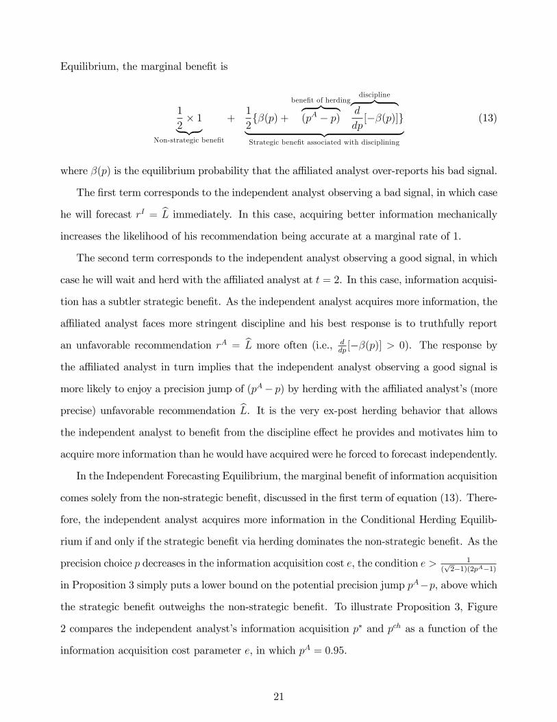
In the Independent Forecasting Equilibrium, the marginal bene�t of information acquisition

comes solely from the non-strategic bene�t, discussed in the �rst term of equation (13). There-

fore, the independent analyst acquires more information in the Conditional Herding Equilib-

rium if and only if the strategic bene�t via herding dominates the non-strategic bene�t. As the

precision choice p decreases in the information acquisition cost e, the condition e > 1(p2�1)(2pA�1)

in Proposition 3 simply puts a lower bound on the potential precision jump pA�p, above which

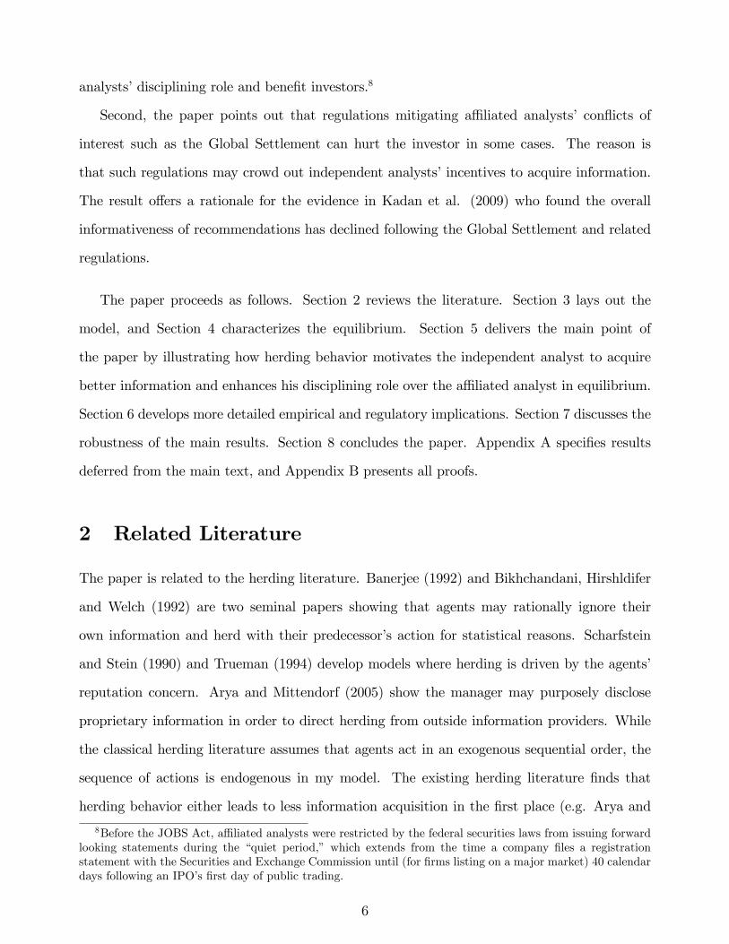
the strategic bene�t outweighs the non-strategic bene�t. To illustrate Proposition 3, Figure

2 compares the independent analyst�s information acquisition p� and pch as a function of the

information acquisition cost parameter e, in which pA = 0:95.

21

1 e*=2.6825 4 60.55

0.65

0.75

0.85

0.95

Information acquisition cost :  e

Info

rmat

ion 

acqu

isiti

on a

t t=0

Figure 2: Herding motivates better information acquisition if  e>e*(pA=0.95)

Conditional Herding Equilibrium

Independent Forecasting Equilibrium

What is the e¤ect of the independent analyst�s herding behavior on the investor�s payo¤?

The answer is not clear at this point: while the independent analyst may acquire better

information in the Conditional Herding Equilibrium (Proposition 3), he sometimes discards

that information and herds with the a¢ liated analyst who by assumption faces a con�ict of

interest. The following proposition summarizes the result.

Proposition 4 (Herding Bene�ts the Investor) Forcing the independent analyst to forecast

independently would make the investor weakly worse-o¤ if and only if the independent analyst�s

informational disadvantage is large, i.e., e > 1(p2�1)(2pA�1) .

The result con�rms the idea that herding per se does not a¤ect the independent analyst�s

disciplining role. Given the a¢ liated analyst�s incentive to over-report a bad signal, the inde-

pendent analyst�s recommendation disciplines the a¢ liated analyst only when it is unfavorable

(rI = bL). In equilibrium, the independent analyst reports his bad signal immediately while heherds only if his private signal is good, which does not compromise his ability to discipline the

a¢ liated analyst. As shown in Proposition 3, if the independent analyst�s informational disad-

vantage is large, his herding strategy motivates better information acquisition and, therefore,

reinforces the disciplining bene�t enjoyed by the investor.

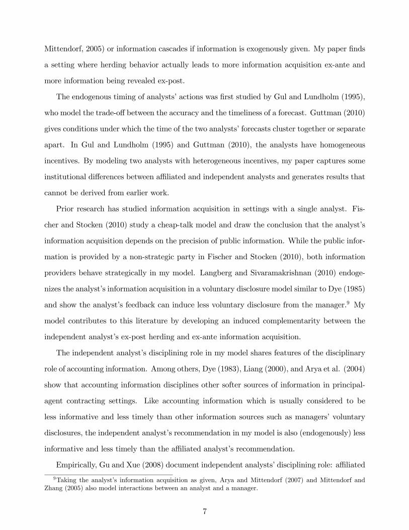
Figure 3 compares the investor�s utility in the Independent Forecasting Equilibrium (the

dotted line) and the Conditional Herding Equilibrium as a function of e. Forcing the indepen-

22

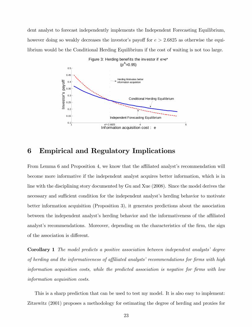
dent analyst to forecast independently implements the Independent Forecasting Equilibrium,

however doing so weakly decreases the investor�s payo¤ for e > 2:6825 as otherwise the equi-

librium would be the Conditional Herding Equilibrium if the cost of waiting is not too large.

1 e*=2.6825 4 60.1

0.15

0.2

0.25

0.3

0.35

0.4

0.45

0.5

Inf ormation acquisition cost :  e

Inve

stor

's p

ayof

fFigure 3: Herding benef its the investor if  e>e*

(pA=0.95)

Conditional Herding Equilibrium

Independent Forecasting Equilibrium

Herding Motivates betterinformation acquisition

6 Empirical and Regulatory Implications

From Lemma 6 and Proposition 4, we know that the a¢ liated analyst�s recommendation will

become more informative if the independent analyst acquires better information, which is in

line with the disciplining story documented by Gu and Xue (2008). Since the model derives the

necessary and su¢ cient condition for the independent analyst�s herding behavior to motivate

better information acquisition (Proposition 3), it generates predictions about the association

between the independent analyst�s herding behavior and the informativeness of the a¢ liated

analyst�s recommendations. Moreover, depending on the characteristics of the �rm, the sign

of the association is di¤erent.

Corollary 1 The model predicts a positive association between independent analysts� degree

of herding and the informativeness of a¢ liated analysts�recommendations for �rms with high

information acquisition costs, while the predicted association is negative for �rms with low

information acquisition costs.

This is a sharp prediction that can be used to test my model. It is also easy to implement:

Zitzewitz (2001) proposes a methodology for estimating the degree of herding and proxies for

23

other variables are common in the existing literature.

The following prediction is about the dynamics of the dispersion of the analysts�recom-

mendations over time.

Corollary 2 The model predicts that the dispersion between independent and a¢ liated ana-

lysts�recommendations decreases over time even if no new information is released.

Traditional wisdom attributes the decrease in the dispersion of analysts�recommendations

to the arrival of new information, which decreases the uncertainty analysts face and leads to

similar opinions. The model o¤ers an alternative and more endogenous explanation. Instead

of relying on exogenous �new�information available from outside, the decrease of dispersion in

my model is caused by how �old�information is gradually comprehended and used over time

inside the analyst market.

The corollary explains O�Brien et al. (2005) and Bradshaw et al. (2006) who �nd that

a¢ liated analysts� recommendations are more optimistic than independent analysts� recom-

mendations only in the �rst several months surrounding IPOs and SEOs, while there is no

di¤erence between the two recommendations made later. According to the model, only the

independent analysts who observe bad signals choose to issue recommendations early, which

explains the a¢ liated analysts�optimism at the beginning. We do not expect any di¤erence

later on because independent analysts who choose to wait will herd with a¢ liated analysts�

recommendations. In addition, since Proposition 4 shows the optimality of the independent

analyst�s herding behavior from the investor�s point of view, my model suggests that the empir-

ical evidence documented above may actually come from the equilibrium (conditional herding

equilibrium) that is favorable to investors. To the best of my knowledge, this prediction has

not been tested outside public o¤ering settings.

The next corollary predicts the coexistence of a¢ liated analysts�optimism and the superi-

ority of their recommendation quality in equilibrium.

Corollary 3 The model predicts that a¢ liated analysts�recommendations are both more opti-

mistic and more informative than independent analysts�recommendations.

24

This prediction is consistent with Dugar and Nathan (1995), Lin and McNichols (1998), and

Gu and Xue (2008).22 The fact that a¢ liated analysts�recommendations are more informative,

together with independent analysts�disciplining e¤ect (see Lemma 6), is also related to Lys

and Sunder (2008). When discussing the disciplining story in Gu and Xue (2008), Lys and

Sunder (2008) raise the question: �It is� therefore� puzzling that the forecasting behavior

of non-independent analysts would vary with the presence of independent analysts who are

inferior forecasters. This raises the question of whether competition from inferior players a¤ects

the behavior of the other incumbent superior players and why such a reaction is rational.�

In my model it is common knowledge that the independent analyst has less precise private

information, and in equilibrium his recommendations are endogenously less informative than

the a¢ liated analyst�s recommendation. Yet, the disciplining role is still present. In other

words, independent analysts can be the inferior forecasters both ex-ante and ex-post, yet still

discipline a¢ liated analysts.

The next corollary addresses a potential, undesirable consequence of regulations such as

the Global Settlement.

Corollary 4 Regulations mitigating the a¢ liated analyst�s con�ict of interest such as the

Global Settlement do not necessarily bene�t the investor.

In the model, a smaller � captures the e¤ect of regulations mitigating the a¢ liated analysts�s

con�ict of interest. While it is easy to show dd�U Inv = 0 in equilibrium (which is driven by

the mixed strategies), the idea that lowering the a¢ liated analyst�s bias does not necessarily

bene�t the investor is more general. In Section 7, I modify the base model so that only pure

strategy equilibria exist and show that lowering the a¢ liated analyst�s con�ict of interest could

strictly decrease the investor�s payo¤. The reason is that the independent analyst tends to put

more trust in the a¢ liated analyst as the latter�s con�ict of interest becomes less severe. It

could be that a smaller � completely wipes out the independent analyst�s incentive to acquire

information ex-ante and therefore the a¢ liated analyst faces no disciplining, in which case the

22See Beyer et al. (2010) and Bradshaw (2011) for a comprehensive review of the mixed evidence on thistopic.

25

investor is worse o¤.23

7 Robustness of Main Results

Due to simpli�cations made for tractability, the a¢ liated analyst and the investor play mixed

strategies in the base model (see Lemma 3). I show in this section that the main results of

the base model are preserved in a game where only pure strategy equilibria exist. To ease

exposition, I restrict the a¢ liated analyst to issuing his recommendation at t = 1 (as in

Subsection 4.1). The goal is to demonstrates that results of the paper are not driven by mixed

strategies.

7.1 Modi�ed setup

Three modi�cations are made to the base model. While the investor is assumed to be risk

neutral with a binary action space fBuy;NotBuyg in the base model, she is now assumed to

be risk averse (CARA utility) and has a continuous action space. The investor is endowed with

e amount of �dollars�which can be invested between a risk-free asset and a risky asset (the

�rm). The return of the risk-free asset is normalized to be zero and the return of the risky

asset is ! 2 fH = 1; L = �1g with the common prior belief that both states are equally likely.

Both assets pay out at the end of the game, and the time value of money is ignored for clean

notation. A portfolio consisting of A units of the risk-free asset and B units of the risky asset

costs the investor A+B �m dollars to form and will generate wealth w to the investor at the

end of the game

w = A+B �m � (1 + !) (14)

where m is the price of the risky asset when the portfolio is formed.24 The investor maximizes

the following utility function

23The reasoning for the second part of Corollary 4 is similar to Fischer and Stocken (2010) who �nd moreprecise public information may completely crowd out an analyst�s information acquisition.24The paper does not model the supply of the share and therefore m is taken as given.

26

U INV = �e���w (15)

where � > 0 is the coe¢ cient of absolute risk aversion. The model does not allow short selling

of the risky asset and therefore B � 0.

The reward the a¢ liated analyst receives for inducing the investor�s buy action is modi�ed

to be proportional to the units of the risky asset the investor buys. If the investor buys B

units of the risky asset, the a¢ liated analyst�s payo¤ function is

UA = Accurate+ ��B (16)

which is a natural extension of UA = Accurate + � � Buy used in the base model as (16)

incorporates the fact that the risk averse investor will buy di¤erent numbers of shares of the

risky asset in response to di¤erent recommendations.

Finally, instead of having a binary support fb; gg in the base model, the a¢ liated analyst�s

private signal yA is now assumed to have a continuous support:

yA = ! + � (17)

where ! 2 fH = 1; L = �1g is the return of the risky asset and the noise term � is normally

distributed

� � N(0; 1) (18)

and the variance of � is normalized to 1 without loss of generality.25

7.2 Equilibrium analysis

As the investor is risk-averse, her holdings of the �rm vary continuously with her posterior

assessment of the �rm. Intuitively, the investor will hold more of the risky asset if her posterior

25The probability density function '(yAj!) satis�es the monotonic likelihood ratio property (MLRP) in thesense that '(y

Aj!=H)'(yAj!=L) increases in y

A.

27

assessment is more optimistic, which is veri�ed by the following lemma.

Lemma 7 In equilibrium, the investor buys B units of the risky asset at a given price m:

B =

8><>:log(

qH1�qH

)

2���m if qH � 12

0 otherwise(19)

and dBdqH

� 0, where qH = Pr(! = HjrA; rI) is derived using Bayesian Rule given the prior

distribution of ! and both analysts�equilibrium strategies.

The following lemma states the properties of the independent analyst�s strategy in equi-

librium. As in the base model (see Proposition 1), the independent analyst observing a good

signal is more likely to wait and herd with the a¢ liated analyst, which opens the gate for the

endogenous timing of the independent analyst�s recommendation.

Lemma 8 In equilibrium, the independent analyst will herd with rA if he keeps silent at t = 1,

and the gain from waiting is higher if he observes a good signal than if he observes a bad signal.

The following lemma shows that the a¢ liated analyst follows an intuitive switching strategy

in equilibrium.

Lemma 9 In equilibrium, the a¢ liated analyst�s strategy is characterized by a unique cut-o¤

point s < 0 such that he forecasts bH if and only if the realization of his signal is greater than

s. Formally, rA = bH , yA > s.

With all players�equilibrium strategies in place, we are ready to present the equilibrium.

Proposition 5 The modi�ed game only has pure strategy equilibria, and the equilibrium takes

one of the following forms

(1) Independent Forecasting Equilibrium where the independent analyst forecasts indepen-

dently at t = 1.

(2) Conditional Herding Equilibrium where the independent analyst forecasts indepen-

dently at t = 1 if and only if his signal is bad while otherwise he waits and herds with the

28

a¢ liated analyst at t = 2.

(3) No Information Acquisition Equilibrium where the independent analyst does not ac-

quire private information and always herds with the a¢ liated analyst�s recommendation at

t = 2.

In any equilibrium, the investor�s investment strategy is de�ned in Lemma 7 and the a¢ liated

analyst follows a switching strategy described in Lemma 9.

As in the base model, the endogenous bene�t of waiting leads to a conditional herding

equilibrium, under which the independent analyst reports his bad signal immediately while he

waits and herds with the a¢ liated analyst otherwise.

The main result of the base model, that herding with the a¢ liated analyst motivates the

independent analyst to acquire more information (Proposition 3) and ultimately bene�ts the

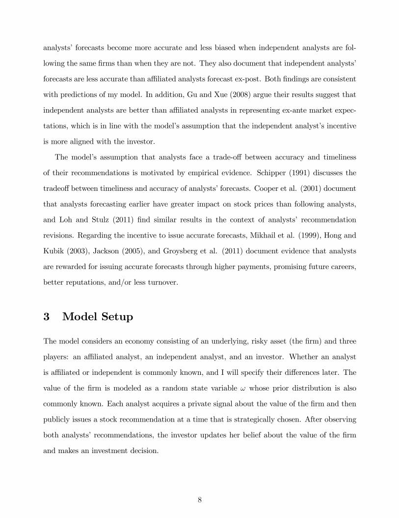
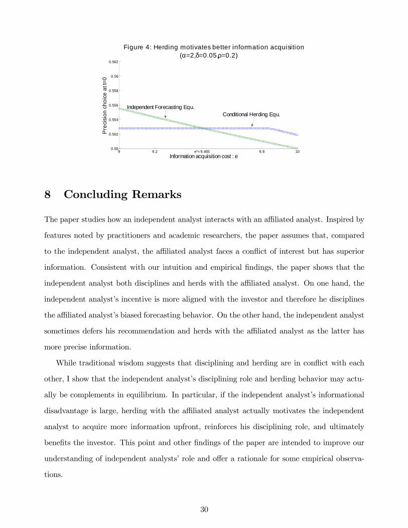
investor (Proposition 4), arises in the modi�ed game as well. Figure 4 plots the precision

chosen by the independent analyst in the Conditional Herding Equilibrium and the Indepen-

dent Forecasting Equilibrium (characterized in Proposition 5) as a function of the information

acquisition cost parameter e, in which � = 2, � = 0:05, and � = 0:2. In this example, the

unique equilibrium of the game is the Conditional Herding Equilibrium for all values of e. It

is clear that the independent analyst acquires better information in the conditional herding

equilibrium than in the Independent Forecasting Equilibrium if his informational disadvantage

is large (e > 9:465 in Figure 4), which is consistent with Proposition 3. One can also check

that the investor is strictly better-o¤ in the Conditional Herding Equilibrium for e > 9:465,

which is consistent with Proposition 4.

29

9 9.2 e*=9.465 9.8 100.55

0.552

0.554

0.556

0.558

0.56

0.562

Information acquisition cost : e

Pre

cisi

on c

hoic

e at

 t=0

Figure 4: Herding motivates better information acquisition(α=2,δ=0.05,ρ=0.2)

Independent Forecasting Equ.Conditional Herding Equ.

8 Concluding Remarks

The paper studies how an independent analyst interacts with an a¢ liated analyst. Inspired by

features noted by practitioners and academic researchers, the paper assumes that, compared

to the independent analyst, the a¢ liated analyst faces a con�ict of interest but has superior

information. Consistent with our intuition and empirical �ndings, the paper shows that the

independent analyst both disciplines and herds with the a¢ liated analyst. On one hand, the

independent analyst�s incentive is more aligned with the investor and therefore he disciplines

the a¢ liated analyst�s biased forecasting behavior. On the other hand, the independent analyst

sometimes defers his recommendation and herds with the a¢ liated analyst as the latter has

more precise information.

While traditional wisdom suggests that disciplining and herding are in con�ict with each

other, I show that the independent analyst�s disciplining role and herding behavior may actu-

ally be complements in equilibrium. In particular, if the independent analyst�s informational

disadvantage is large, herding with the a¢ liated analyst actually motivates the independent

analyst to acquire more information upfront, reinforces his disciplining role, and ultimately

bene�ts the investor. This point and other �ndings of the paper are intended to improve our

understanding of independent analysts�role and o¤er a rationale for some empirical observa-

tions.

30

The main point that herding can motivate better information acquisition and reinforce

disciplining seems likely to apply to settings other than a¢ liated and independent analysts.

For example, mutual fund managers base their portfolio choices on both buy-side and sell-side

analysts�forecasts. While sell-side analysts potentially face con�icts of interest such as trade-

generating incentives, it has been documented that their forecasts are more precise than buy-

side analysts (e.g., Chapman et al., 2008). The paper suggests that buy-side analysts may serve

a disciplinary role. Moreover, in order to induce buy-side analysts to acquire more information,

fund managers may purposely allow buy-side analysts to herd with sell-side analysts by passing

along the latter�s forecast to buy-side analysts.

31

References

[1] Arya, A., Glover, J., Mittendorf, B. and Zhang, L., 2004. The disciplining role of account-

ing in the long-run. Review of Accounting Studies 9: 399-417.

[2] Arya, A. and Mittendorf, B., 2005. Using disclosure to in�uence herd behavior and alter

competition. Journal of Accounting and Economics 40, 231�246.

[3] Arya, A. and Mittendorf, B., 2007. The interaction among disclosure, competition between

�rms, and analyst following. Journal of Accounting and Economics 43, 321�339.

[4] Banerjee, A. V., 1992. A Simple Model of Herd Behavior. Quarterly Journal of Economics,

107, 797�817.

[5] Beyer, A., Cohen, D., Lys, T., andWalther, B., 2010. The �nancial reporting environment:

Review of the recent literature. Journal of Accounting and Economics 50, 296-343.

[6] Bikhchandani, S., Hirshleifer, D. and Welch, I., 1992. A Theory of Fads, Fashion, Custom,

and cultural Change as Informational Cascades. Journal of Political Economy, 100, 992�

1026.

[7] Bradshaw, M. T., 2011. Analysts�Forecasts: What Do We Know after Decades of Work?

Working Paper.

[8] Bradshaw, T. M, Richardson, A. S., and Sloan, G. R., 2006. The relation between corpo-

rate �nancing activities, analysts�forecasts and stock returns. Journal of Accounting and

Economics 42, 53-85.

[9] Chapman, C., Healy, P. and Groysberg, B., 2008. Buy-Side vs. Sell-Side Analysts�Earnings

Forecasts. Financial Analysts Journal, 64: 25-39.

[10] Chen, T. and Martin, X., 2011. Do bank-a¢ liated analysts bene�t from lending relation-

ships? Journal of Accounting Research, 49: 633-674.

32

[11] Cho, I. and Kreps, D. M., 1987. Signaling games and stable equilibria. Quarterly Journal

of Economics, 102:179-221.

[12] Cooper, R. A., Day, T. E., and Lewis, C. M., 2001. Following the leader: A study of

individual analysts�earnings forecasts. Journal of Financial Economics, 61: 383-416.

[13] Dugar, A. and Nathan, S., 1995. The e¤ect of investment banking relationships on �nancial

analysts�earnings forecasts and investment recommendations. Contemporary Accounting

Research 12, 131�160.

[14] Dye, R. A., 1983. Communication and post-decision information. Journal of Accounting

Research 21:514-533.

[15] Dye, R. A., 1985. Disclosure of nonproprietary information. Journal of Accounting Re-

search 23: 123-145.

[16] Fischer, P. E. and Stocken, P. C., 2010. Analyst information acquisition and communica-

tion. The Accounting Review 85, 1985-2009.

[17] Fudenberg, D. and Tirole, J., 1991. Game Theory. The MIT Press.

[18] Groysberg, B., Healy, P. M. and Maber, D. A., 2011. What drives sell-side analyst compen-

sation at high-status investment banks? Journal of Accounting Research, 49: 969-1000.

[19] Gu, Z. and Wu, J. 2003. Earnings skewness and analyst forecast bias. Journal of Account-

ing and Economics, 35: 5-29.

[20] Gu, Z. and Xue, J., 2008. The superiority and disciplining role of independent analysts.

Journal of Accounting and Economics, 45: 289-316.

[21] Gul, F. and Lundholm,R., 1995. Endogenous timing and the clustering of agents�decisions.

Journal of Political Economy 103, 1039�1066.

[22] Guttman, I., 2010. The timing of analysts�earnings forecasts. The Accounting Review 85,

513�545.

33

[23] Hirshleifer, D. and Teoh, S. H., 2003. Herding behavior and cascading in capital markets:

a review and synthesis. European Financial Management, 9: 25-66.

[24] Hong, H. and Kubik, J., 2003. Analyzing the analysts: career concerns and biased earnings

forecasts. The Journal of Finance 58, 313�351.

[25] Irvine, P., 2004. Analysts�forecasts and brokerage-�rm trading. The Accounting Review

79: 125�149.

[26] Jackson, A., 2005. Trade generation, reputation, and sell-side analysts. The Journal of

Finance 60, 673�717.

[27] Jacob, J., Rock, S. and Weber, D., 2008. Do non-investment bank analysts make better

earnings forecasts? Journal of Accounting, Auditing and Finance 23: 23�60.

[28] Kadan, O., Madureira, L., Wang, R. and Zach, T., 2009. Con�ict of interest and stock

recommendations: the e¤ects of the global settlement and related regulations. Review of

Financial Studies, 22: 4189-4217.

[29] Langberg, N. and Sivaramakrishnan, K., 2010. Voluntary disclosures and analyst feedback.

Journal of Accounting Research 48: 603-646.

[30] Liang, P., 2000. Accounting recognition, moral hazard, and communication. Contemporary

Accounting Research 17, 457-490.

[31] Lin, H. and McNichols, M., 1998. Underwriting relationships, analysts�earnings forecasts

and investment recommendations. Journal of Accounting and Economics 25, 101�127.

[32] Loh, R. K., and Stulz, R. M., 2011. When are analyst recommendation changes in�uential?

Review of Financial Studies, 24: 593-627.

[33] Lys, T. Z. and Sunder, J., 2008. Endogenous entry/exit as an alternative explanation for

the disciplining role of independent analyst. Journal of Accounting and Economics, 45:

317-323.

34

[34] Michaely, D., and Womack, K., 1999. Con�ict of interest and the credibility of underwriter

analyst recommendations. Review of Financial Studies, 12: 653�686.

[35] Mikhail, B. M., Walther, B. R. and Willis, R. H., 1999. Does Forecast Accuracy Matter

to Security Analysts?. The Accounting Review, 74: 185�200.

[36] Mittendorf, B. and Zhang, Y., 2005. The role of biased earnings guidance in creating a

healthy tension between managers and analysts. The Accounting Review 80, 1193�1209.

[37] Mola, S., and Guidolin, M., 2009. A¢ liated mutual funds and analyst optimism. Journal

of Financial Economics, 93: 108-137.

[38] O�Brien, P., McNichols, M. and Lin, H., 2005. Analyst impartiality and investment bank-

ing relationships. Journal of Accounting Research 43, 623�650.

[39] Scharfstein, D. S. and Stein, J. C., 1990. Herd behavior and Investment. American Eco-

nomic Review, 80: 465-479.

[40] Schipper, K., 1991. Analysts�forecasts. Accounting Horizon, 5: 105-131.

[41] Trueman, B., 1994. Analyst forecasts and herding behavior. Review of Financial Studies,

7: 97-124.

[42] Van Campenhout, G. and Verhestraeten, J. 2010. Herding Behavior among Financial

Analysts: A Literature Review. Working paper.

[43] Welch, I., 2000. Herding among security analysts. Journal of Financial Economics, 58:

369-396.

[44] Zitzewitz, E., 2001. Measuring herding and exaggeration by equity analysts and other

opinion. Working paper.

[45] Zhang, J., 1997. Strategic delay and the onset of investment cascades. Rand Journal of

Economics, 28: 188-205.

35

Appendix A

Equilibrium for � > � and � < �

(i) For � > �, the game has an equilibrium in which the a¢ liated analyst issues a �xed

recommendation at t = 1, that is rA � bL or rA � bH. The independent analyst choosesp� = 1+e

2eand forecasts independently at t = 1, that is rI = bH , yA = g. The investor bases

her investment decision on rI alone unless the a¢ liated analyst makes an out-of-equilibrium

recommendation, in which case the investor does not buy.

(ii) For � < 2pA� 1, the game has an equilibrium in which the a¢ liated analyst truthfully

reports his signal at t = 1, i.e., rA = bH , yA = g. For � � � � � = 2pA� 1+ �, the game has

an equilibrium in which the a¢ liated analyst perfectly signals his signal by the timing of his

recommendation: he issues bH at t = 2 upon observing a good signal while otherwise he issuesbL at t = 1. The independent analyst chooses precision p� = 1+e2eand forecasts independently

at t = 1 if � > pA� (p� � c(p�)) while otherwise he acquires no information and herds with rA

at t = 2. The investor bases her investment on rA alone.

Details of the additional equilibria summarized in Lemma 5

For � < b�, the a¢ liated analyst issues his recommendation at t = 2 while the independentanalyst chooses precision p� = 1+e

2eand forecasts independently at t = 1. Particularly,

(i) If � � pA+p��11�pA+2pAp��p� and � <

b�, the a¢ liated analyst issues bL if and only if both yA = band rI1 = bL, and the investor buys if and only if the a¢ liated analyst issues bH at t = 2.

(ii) If � > pA+p��11�pA+2pAp��p� and � <

b�, the a¢ liated issues rA = bH unless both his signal is

bad and the independent analysts issues bL, in which case the a¢ liated analyst issues bH with

probability � = pH�p�pH+p��1 . The investor bases her investment decision on r

A unless rA = bH but

rI = bL, in which case she does not buy with probability 1� 1�p��pH�(pH+p��1�2pHp�) .

In both cases, the investor will not buy if the a¢ liated analyst forecasts at t = 1 (the

out-of-equilibrium path). Constants b� = p� + p��+ pA(�� 2p��� 1).

36

Appendix B

Notation: pA (p) is the precision of the a¢ liated (independent) analyst�s signal yA (yI);

� is the cost of deferring a recommendation, e is the information acquisition cost parameter,

and � measures the a¢ liated analyst�s degree of con�ict of interest.

Proof of Lemma 1. Denote �(p) := Pr(rA = bHjyA = b; p) and (p) := Pr(rA = bLjyA = g; p),I will show that in equilibrium (p) = 0. The argument holds for all p and therefore I will

write � and for simplicity. Denote I bH = Pr(! = HjrA = bH) and IbL = Pr(! = LjrA = bL)as the informativeness of rA = bH and rA = bL respectively. Notice I bH ; IbL 2 [1 � pA; pA] arewell-de�ned as � � � guarantees both rA = bL and rA = bH can be observed in equilibrium. It

is an important observation that

(I bH � 12)(IbL �1

2) =

(2pA � 1)2(� + � 1)24 (1� ( � �)2) � 0

and that I bH = 12, IbL = 1

2, � + = 1.

First, I claim that I bH = 12(thus IbL = 1

2) cannot hold in equilibrium. Suppose the opposite

is true, then both rA = bH and rA = bH are ignored by the investor, which means that the

a¢ liated analyst is strictly better o¤ by forecasting truthfully, i.e., rA = bH if and only if

yA = g. However the truthful reporting strategy implies I bH = IbL = pA and contradicts I bH =IbL = 1

2. Since I bH = 1

2cannot be part of an equilibrium, we are left with two possible scenarios:

I bH ; IbL < 12or I bH ; IbL > 1

2.

Next, I claim that I bH ; IbL < 12cannot hold in equilibrium. Suppose by contradiction that

in equilibrium IbL < 12and I bH < 1

2. Given yA = b, the a¢ liated analyst�s payo¤ is pA + � �

EhBuyjyA = b; rA = bLi if he forecasts rA = bL, and is 1� pA + � �E hBuyjyA = b; rA = bHi if

rA = bH. The expectation operatorE[�jyA; rA] is taken over yI , taking the independent analyst�sstrategy and the investor�s strategy as given. The independent analyst�s payo¤ function (7)

guarantees that in equilibrium his strategy must satisfy I bH < 12) Pr(rI = bHjyI ;Time) �

Pr(rI = bHjyI ;Time)8yI . The Time parameter re�ects that whether the independent analyst�sinformation set contains rA depends on the timing of his recommendation (or waiting strategy),

37

which is measurable only with respect to yI and cannot depend on rA. In addition, the investor�s

payo¤ function (8) guarantees that in equilibrium her strategy must be such that I bH < 12)

Pr(BuyjrI ; rA = bH) � Pr(BuyjrI ; rA = bL)8rI . Given such properties of the independentanalyst�s strategy and the investor�s strategy, we have I bH < 1

2) E

hBuyjyA = b; rA = bHi �

EhBuyjyA = b; rA = bLi in equilibrium, andI bH < 1

2) pA + � � E

hBuyjyA = b; rA = bLi > 1� pA + � � E hBuyjyA = b; rA = bHi :

Therefore I bH < 12implies that forecasting bL must be a dominant strategy in equilibrium for

the a¢ liated analyst if yA = b. This implies �(p) = 0 for 8p and thus IbL � 12, a contradiction

to the assumption that IbL < 12.

Finally we are left with I bH ; IbL > 12and I claim that (p) = 0 in equilibrium. Following

the similar argument developed above, one can show I bH > 12) E

hBuyjyA = g; rA = bHi �

EhBuyjyA = g; rA = bLi andI bH > 1

2) pA + � � E

hBuyjyA = g; rA = bHi > 1� pA + � � E hBuyjyA = g; rA = bLi :

Therefore, in any equilibrium with I bH > 12, rA = bH is the a¢ liated analyst�s strict best

response upon observing yA = g, and this proves the claim (p) = 0.

Proof of Lemma 2. The lemma is surely true if the independent analyst�s private signal

yI and the a¢ liated analyst�s recommendation rA imply the same recommendation, so what

is left is the case when yI and rA imply di¤erent recommendations. Suppose by contradiction

that the independent analyst will stick to yI if rA implies di¤erently, which means after all he

forecasts independently in the sense that rI = bL if and only if yI = b. But there is a pro�tabledeviation for the the independent analyst by simply forecasting independently at t = 1 and

avoiding the waiting cost �, a contradiction.

Proof of Proposition 1.

Consider the case in which both rA = bH and rA = bL are on the equilibrium path. After

38

observing yI 2 fg; bg with precision p, the independent analyst will obtain expected utility

p+ �� c(p) if he forecasts immediately. On the other hand, if he defers his recommendation to

t = 2 in equilibrium, we know by Lemma 2 that he will herd with rA at t = 2. Let E�GainjyI

�be the expected informational gain from deferring a recommendation given yI , we have

E�GainjyI = b

�= p(1� �)pA + (1� p)

�pA + (1� pA)�

�� (p+ �)

E�GainjyI = g

�= p

�pA + (1� pA)�

�+ (1� p)(1� �)pA � (p+ �):

where � = Pr(rA = bHjyA = b) is the probability that the a¢ liated analyst over-reports a badsignal, and we know from Lemma 1 that we can ignore the under-reporting strategy as long as

both rA = bH and rA = bL can be observed in equilibrium. It is easy to check thatE�GainjyI = g

�� E

�GainjyI = b

�= (2p� 1)� � 0:

If only rA = bH (or rA = bL) is reported on the equilibrium path, then rA is uninformative

and the gain from observing it is zero for the independent analyst regardless of his signal yI .

Proof of Lemma 3. First, I show that, in equilibrium, the independent analyst will not defer

his recommendation upon observing yI = b. Suppose by contradiction this is not the case. Then

the independent analyst will also defer his recommendation upon observing yI = g. The result

is the independent analyst will unconditionally defer his recommendation, and (by Lemma 2)

herd with the a¢ liated analyst�s recommendation rA. Knowing this, the a¢ liated analyst will

forecast rA = bH for all yA, which makes his recommendation completely uninformative and

contradicts the assumption that the independent analyst chooses to herd in the �rst place.

Upon observing yI = g, the independent analyst will either forecast bH if he chooses to

forecast at t = 1, or herd with rA at t = 2 if he chooses to defer (by Lemma 2).

Given the independent analyst�s forecasting strategy and p > 12, the a¢ liated analyst sets

� = Pr(rA = bHjyA = b) = pA�ppA+p�1 so that the investor is indi¤erent from �Buy�and �Not Buy�

39

upon observing rA = bH but rI = bL. The investor, upon observing rA = bH but rI = bL, choosesnot to buy with probability � = ��(2pA�1)

�(1�pA�p+2pAp) so that the a¢ liated analyst is indi¤erent

between reporting bH and bL upon observing a bad signal yA = b. One can see that 0 � � � 1is guaranteed in the non-trivial region � � � � �.

Given yI = g, the independent analyst obtains an expected payo¤ p+��c(p) if he forecasts

early, while his expected payo¤ from waiting (and herding with rA) is p�pA + (1� pA)�

�+

(1�p)(1��)pA� c(p). Substituting � from above, simple algebra shows that the independent

analyst will forecast his good signal at t = 1 if and only if

� � (pA � p)(2p� 1)pA + p� 1 :

Collecting conditions completes the proof.

Proof of Proposition 2. Denote p� (pch) as the optimal precision the independent analyst

chooses if the equilibrium of the overall game is the Independent Forecasting Equilibrium (and

the Conditionally herd equilibrium). Then p� satis�es

p� = argmaxp2[ 1

2;1]

p+ � � e� (p� 12)2; (20)

which gives p� = 1+e2e. pch satis�es

pch 2 argmaxp

1

2(p+ �) +

1

2

�p(pA + (1� pA)�) + (1� p)(1� �)pA

�� e(p� 1

2)2:

pch is solved from the following f.o.c

e� 2e� pch + (2pA � 1)22(pA + pch � 1)2 = 0: (21)

Since pA + pch � 1 > 0, pch can be solved equivalently from the following cubic function

2(pA + pch � 1)2(e� 2e� pch) + (2pA � 1)2 = 0:

40

This equation has a unique real root and two complex conjugate roots for any pA > 12,26 and

it is easy to check the second-order condition is �2e� (2pA�1)2(pA+p�1)3 < 0.

The independent analyst�s expected payo¤ at t = 0, after plugging in p� and pch, is de-

noted as U IIF in the Independent Forecasting Equilibrium and UICH in the Conditional Herding

Equilibrium. Simple algebra shows that

U ICH > UIIF , � < �;

where

� =4pApch � pA � pchpA + pch � 1 � e

2(1� 2pch)2 + 2e+ 12e

:

Together with the self-ful�lling conditions characterized in Lemma 3, one can see the overall

equilibrium is the Conditional Herding Equilibrium if � is in the following set

�� : � < min

�� ;

(pA � pch)(2pch � 1)pA + pch � 1

��= f� : � < �g ;

where the equality is by straightforward algebra (pA�pch)(2pch�1)pA+pch�1 � � = (2epch�1)2

2e> 0.

Analogously, the overall equilibrium is the Independent Forecasting Equilibrium if � is in

the following set �� : � > max

�� ;

(pA � p�)(2p� � 1)pA + p� � 1

��;

and the remainder of the proof is to show� � (pA�p�)(2p��1)pA+p��1 , which meansmax

�� ; (p

A�p�)(2p��1)pA+p��1

�=

� and veri�es the proposition.

Proving � � (pA�p�)(2p��1)pA+p��1 follows the graphic investigation of three claims. Claim 1: Both

� and �� := (pA�p�)(2p��1)pA+p��1 strictly increase in e for e < e� while strictly decreases in e for e >

e� (where e� = 1(p2�1)(2pA�1)). Claim 2: � and �� achieve the same global maximum value at

e = e�, i.e., max� = �(e = e�) = ��(e = e�) = max ��. Claim 3:��d��de

�� > ��d�de

�� holds for e < e�and e > e�.26by investigating the discriminant of the cubic function. See Chapter 10 of the book Integers, Polynomials,

and Rings: A Course in Algebra by Ronald S. Irving.

41

Proof of Claim 1: For the �� part, �rst notice that �(p) = (pA�p)(2p�1)pA+p�1 is strictly concave

in p and d�dp> 0 if and only if p < 1 � pA + 2pA�1p

2. As p� = 1+e

2eand dp�

de< 0, we know

p� < 1 � pA + 2pA�1p2if and only if e > e� = 1

(p2�1)(2pA�1) . Finally, since �

� = (pA�p�)(2p��1)pA+p��1 =

�(p = p�), the claim for �� is true by applying the Chain Rule d��

de= d��

dp�dp�

deand the fact that

dp�

de< 0.

For the � part, rewrite � as �(e; pch(e)) to emphasize that its second argument pch is also

a function of e. Di¤erentiating �(e; pch(e)) with respect to e,

d

de�(e; pch(e)) =

@�(e; pch(e))

@e+@�(e; pch(e))

@pchdpch

de:

Notice that@�(e; pch(e))

@pch= 2(e� 2epch) + (2pA � 1)2

(pA + pch � 1)2 = 0:

The last equality comes from the fact that pch is the optimal precision chosen in the conditional

herding equilibrium, and by (21) that pch satis�es

e� 2epch + (2pA � 1)22(pA + pch � 1)2 = 0:

Therefore, dde�(e; pch(e)) can be simpli�ed as

d

de�(e; pch(e)) =

@�(e; pch(e))

@e

=1

2(1

e2� (2pch � 1)2):

Straightforward calculus shows

d�

de> 0, pch <

1 + e

2e:

We know from Proposition 3 that pch < 1+e2e= p� if and only if e < e�. Monotonic transforma-

tion givesd�

de> 0, e < e�:

42

which veri�es Claim 1.

Proof of Claim 2: As both � and �� are continuous functions, the fact that they achieve

their global maximum value at e = e� is a direct consequence of Claim 1. We know by

Proposition 3 that p� = pch = 1 � pA + 2pA�1p2at e = e�. Substituting p� and pch veri�es the

claim.

Proof of Claim 3: We know from Claim 1 that d�decan be simpli�ed as 1

2( 1e2� (2pch�1)2),

and algebra shows that d��

de= 1�e(2+e(2pA�1)2�4pA)

e2(e�1�2epA)2 . Simple algebra shows

dif =d�

de� d�

�

de

= �2pch2 + 2pch � 12+

32+ 2

(�1+e�2epA)2 �4

1�e+2epA

e2:

Evaluating dif at e = e� we know dif(e = e�) = 0, where the last equation uses the result

from Proposition 3 that pch = p� = 1 � pA + 2pA�1p2at e = e�. Since dif is quadratic in pch

which is positive by de�nition, it is easy to verify that

dif � 0, pch � 1� pA + 2pA � 1p2

:

Applying the Implicit Function Theorem to the f.o.c de�ning pch, we have

dpch

de=

1� 2pch

2e+ (2pA�1)2(pA+pch�1)3

< 0:

Monotonic transition gives

dif � 0, e � e�:

which, together with Claim 1, veri�es the claim.

Finally pch 2 (12; pA) is easy to show by combining the fact dpch

de< 0 and the results of

Proposition 3.

Proof of Lemma 4. One can verify the lemma by replicating the proof of Proposition

2 (players assigning probability one to yA = b on the out-of-equilibrium path supports the

43

equilibrium). The remainder shows that the speci�ed out-of-equilibrium belief satis�es both

the Intuitive Criterion and the Universal Divinity Criterion.

For the purpose of equilibrium re�nement, it is su¢ cient to check beliefs assigned to the

a¢ liated analyst�s out-of-equilibrium messages only.27 As the a¢ liated analyst forecasts at

t = 1 in equilibrium, the game has two out-of-equilibrium messages: rA = bH at t = 2

and rA = bL at t = 2, which are denoted as rA2 = bH and rA2 = bL.Universal Divinity Criterion: I illustrate the argument for the out-of-equilibrium mes-

sage rA2 = bH (referred as m for short), and the argument for rA2 = bL is similar.Some notation is necessary to apply the criterion. Let BR(�; rI ;m) be the investor�s pure-

strategy best response to the out-of-equilibrium messagem, given the belief � over the a¢ liated

analyst�s type (his signal yA 2 fg; bg) and the independent analyst�s recommendation rI .

Similarly let MBR(�; rI ;m) be the set of mixed-strategy best response to m, given � and rI ,

that is the set of all probability distributions over BR(�; rI ;m).

Then de�ne D(t; T;m) to be the set of the investor�s mixed-strategy best responses to the

out-of-equilibrium message m and beliefs concentrated on support of a¢ liated analyst�s type

space T that makes type t 2 fg; bg strictly prefer m to his equilibrium payo¤.

D(t; T;m) = [f�:�(T )=1g

fx 2MBR(�; rI ;m)s:t:u�(t) < u(m;x; t)g: (22)

where x := Pr(Buyjm) is the probability that the investor buys the stock upon observing the

out-of-equilibrium message m, u�(t) is the type-t a¢ liated analyst�s payo¤ on the equilibrium

path, u(m;x; t) is type-t�s expected payo¤ by sending out m when the investor reacts to it

with x, and � = Pr(yA = gjm) is the investor�s belief that the a¢ liated analyst is good type.

Similarly let D0(t; T;m) be the set of mixed best responses that make type t exactly indi¤erent.

Finally, D(t; T;m) and D0(t; T;m) are functions of rI , which I will return to later.

Algebra shows that the good type a¢ liated analyst (with yA = g) prefers the out-of-

equilibriummessage rA2 = bH to his equilibrium action if x > (2pA�1)[�+e2pA+e(2pA+2p(1+��2pA)��)]+�(2pA�1+e)�

:=

27Since the independent analyst�s payo¤ does not depend on the investor�s action, one can assign arbitrarybeliefs to his out-of-equilibrium actions and those beliefs will survive both equilibrium re�nement criteria usedin the paper.

44

A, where p 2 fp�; pchg is the independent analyst�s precision choice in equilibrium. Likewise,

the bad type a¢ liated analyst (with yA = b) prefers sending out rA1 = bH if x > 2pA�1+��

.

Furthermore, the following is true under the maintained assumption � > � (see (11))

A > B: (23)

Now calculate MBR(�; rI ;m), the investor�s mixed-strategy best response. Notice the in-

vestor�s best response depends not only on her belief about the a¢ liated analyst�s type, but

also on the independent analyst�s recommendation. Denote ��(rI = bL) as the probability ofyA = g such that the investor is indi¤erent about buying or not buying upon observing rI = bL;and similarly ��(rI = bH) as the probability of yA = g such that the investor is indi¤erent

about buying or not buying upon observing rI = bH. Clearly��(rI = bH) < ��(rI = bL):

The set of investor�s mixed best response MBR(�; rI ;m) is

MBR(�; rI ;m) =

8>>>>>>>>>>>>>>>>>>>><>>>>>>>>>>>>>>>>>>>>:

x = 0 if � < ��(rI = bH)x 2 [0; 1] if � = ��(rI = bH) and rI = bHx = 0 if � = ��(rI = bH) and rI = bLx = 0 if ��(rI = bH) < � < ��(rI = bL) and rI = bLx = 1 if ��(rI = bH) < � < ��(rI = bL) and rI = bHx = 1 if � = ��(rI = bL) and rI = bHx 2 [0; 1] if � = ��(rI = bL) and rI = bLx = 1 if � > ��(rI = bL):

45

Therefore

D(g; T;m) = [f�:�(T )=1g

fx > A \MBR(�; rI ;m)g

=

8><>: x > A if rI = bHx > A if rI = bL

= x > A:

To understand the second equality, note that set MBR(�; rI ;m) inside the union operation

depends on both � and rI while the union is taken only with respect to �, and therefore the

outcome is a function of rI . The last equality shows that the set D(good; T;m) degenerates to

a deterministic set.

Similarly, one can show that D(b; T;m) is as follows:

D(b; T;m) = [f�:�(T )=1g

fx > B \MBR(�;m)g

=

8><>: x > B if rI = bHx > B if rI = bL

= x > B:

As we know from (23) A > B, we have

D(good; T;m) [D0(good; T;m) � D(bad; T;m): (24)

According to the Universal Divinity Criterion, (24) means the equilibrium should assign proba-

bility zero to type yA = g upon observing the out-of-equilibrium messagem, which is consistent

with the strategy speci�ed in Lemma 4.

Intuitive Criterion: On one hand, suppose players assign probability one to yA = g upon

observing any of the two out-of-equilibrium messages rA2 = bH and rA2 = bL. Given the proposedbelief, it is easy to show that the a¢ liated analyst observing yA = b (bad-type) is strictly better

o¤ by sending out either of the two out-of-equilibrium messages than choosing his equilibrium

46

action. This implies that neither of the out-of-equilibrium messages can be eliminated for the

bad-type a¢ liated analyst by equilibrium dominance used in the Intuitive Criterion (Cho and

Kreps, 1987 Page 199-202). On the other hand, even if any of the out-of-equilibrium messages

can be eliminated for the good-type (yA = g) a¢ liated analyst, the bad-type a¢ liated analyst

does not have incentive to send out that message and being identi�ed.

Proof of Lemma 5. Recall that the details of the additional equilibrium are stated in

Appendix A.

Part (i): � � pA+p��11�pA+2pAp��p� ensures that it is a strict best response for the a¢ liated analyst

to issue bL upon observing both yA = b and rI1 = bL. � � b� prevents the a¢ liated analyst fromdeviating the equilibrium by issuing recommendations at t = 1. It is then easy to verify the

equilibrium.

Part (ii): � = pA�p�pA+p��1 is chosen so that the investor is indi¤erent between "Buy" and

"Not Buy" after observing frA = bH \ rI = bLg. Likewise, � = 1� 1�p��pA�(pA+p��1�2pAp�) is chosen so

that a¢ liated analyst is indi¤erent between issuing bH and bL when observing fyA = b; rI = bLg,and 0 � � � 1 requires � > pA+p��1

1�pA+2pAp��p� . Substituting � and �, one can show � <b� prevents

the a¢ liated analyst from deviating the equilibrium by issuing recommendations at t = 1.

Proof of Lemma 6. Recall that � = pA�ppA+p�1 in both the Conditional Herding Equilibrium

and the Independent Forecasting Equilibrium. Simple algebra veri�es the Lemma.

Proof of Proposition 3. From the Proof of Proposition 2 we know p� = 1+e2ewhile pch

maximizes

U(p) =1

2p+

1

2

�p(pA + (1� pA)�) + (1� p)(1� �)pA � �

�� e(p� 1

2)2

and U 0(p)jp=pch = 0. Also, it is easy to show

U 00(p) = �2e� (2pA � 1)2(pA + p� 1)3 < 0:

47

Therefore, U 0(p) is strictly decreasing with respect to p. Evaluating U 0(p) at p = p�, we obtain

U 0(p)jp=p� =2(2epA � e)2(2epA � e+ 1)2 � 1:

Algebra shows

U 0(p)jp=p� > 0 = U 0(p)jp=pch , e >1

(p2� 1)(2pA � 1)

:

Since U 00(p) < 0, U 0(p)jp=p� > U 0(p)jp=pch implies p� < pch. Therefore,

pch > p� , e >1

(p2� 1)(2pA � 1)

:

This completes the proof.

Proof of Proposition 4. Denote peq as the precision acquired by the independent analyst

in equilibrium, which is given in Proposition 2, one can show the investor�s equilibrium payo¤

is

U Inv(peq) =(2pA � 1)(2peq � 1)2(pA + peq � 1)

andd

dpeqU Inv(peq) > 0:

This inequality, together with Proposition 3, completes the proof.

Proof of Lemma 6. � = pA�ppA+p�1 , and simple algebra veri�es the Lemma.

Proof of Corollary 1. Direct implication of Proposition 3

Proof of Corollary 2. The dispersion of analysts�recommendation is the ex-ante percentage

that two analysts�recommendation are di¤erent ( bH versus bL) among all the recommendationsobserved by the investor up to period t. In the Conditional Herding Equilibrium, one can

show Dispersion1 =Pr(rA= bH;yI=b)

Pr(yI=b)and Dispersion2 = Pr(rA = bH; yI = b), where the subscript

represents period t. It is clear that Dispersion1 > Dispersion2.

Proof of Corollary 3. By the proof of Lemma 3, we know in equilibrium Pr(! = HjrA =bH) = p and Pr(! = LjrA = bL) = pA. Since rA = bL happens with strictly positive probability48

and pA > p, the overall (ex-ante) informativeness of the a¢ liated analyst�s recommendation is

higher than that of the independent analyst. From the ex-ante perspective, Pr(rA = bH) > 12

while Pr(rI = bH) � 12, and therefore in equilibrium we observe the a¢ liated analysts issue

favorable recommendations more often.

Proof of Lemma 7. Given the investor�s endowment is e, holding y units of risky asset and

x units of risk-free asset will generate wealth w

w = (1 + !) �m � y + x

= (1 + !) �m � y + e�m � y

= ! �m � y + e:

The second equality makes uses of the budget constraint e = m � y + x. The optimal holding

B is

B = argmaxy�0

qH � �e���(e+my) + (1� qH)� e���(e�my);

where qH = Pr(! = HjrA; rI) is the posterior probability of ! = H. Solving the program we

obtain

B =

8><>:log(

qH1�qH

)

2���m if qH � 12

0 otherwise.

Simple algebra veri�es the lemma.

Proof of Lemma 8. The proof of Lemma 2 can be used to prove the �rst part of the lemma.

To show the second part of the lemma, let us �rst state a necessary condition for the a¢ liated

analyst�s strategy to be in equilibrium. Point-wise mappings �(yA; p) := Pr(rA = bHjyA; p) and (yA; p)

:= Pr(rA = bLjyA; p) for 8yA;8p characterize the a¢ liated analyst�s strategy, and I will

write �(yA) and (yA) for short as the argument below holds for all p. The informativeness of

49

rA is calculated as follows

I bH = Pr(! = HjrA = bH) = R +1�1 �(yA)'Hdy

AR +1�1 �(yA)'Hdy

A +R +1�1 �(yA)'Ldy

A

IbL = Pr(! = LjrA = bL) = R +1�1 (yA)'Ldy

AR +1�1 (yA)'Ldy

A +R +1�1 (yA)'Hdy

A:

where 'H and 'L are the probability density function of yA conditional on state ! = H and

L. One can show that

(I bH � 12)(IbL �1

2) � 0

and (I bH � 12)(IbL � 1

2) = 0,

R +1�1 �(yA)'Hdy

A =R +1�1 �(yA)'Ldy

A , I bH ; IbL = 12. Arguments

developed in Lemma 1 can be used to show that (1) in equilibrium I bH ; IbL > 12, and (2) in

equilibrium rA = bH is the a¢ liated analyst�s strict best response for any yA � 0 and therefore

�(yA) = 1;8yA � 0 in equilibrium. (25)

Now turn to the independent analyst�s expected payo¤ by deferring his forecast to t = 2

after observing a signal yI with precision p, denoted as U It2(yI ; p). We know that waiting implies

subsequent herding in equilibrium. Therefore

U It2(b; p) = p �Z +1

�1 (yA)'Ldy

A + (1� p)Z +1

�1�(yA)'Hdy

A

U It2(g; p) = p �Z +1

�1�(yA)'Hdy

A + (1� p)Z +1

�1 (yA)'Ldy

A;

50

and

U It2(g; p)� U It2(b; p) = (2p� 1)�Z +1

�1�(yA)'Hdy

A �Z +1

�1 (yA)'Ldy

A

�= (2p� 1)

�Z +1

�1�(yA)'Hdy

A +

Z +1

�1�(yA)'Ldy

A � 1�

� (2p� 1)�Z +1

0

�(yA)'HdyA +

Z +1

0

�(yA)'LdyA � 1

�= (2p� 1)

�Z +1

0

'HdyA +

Z +1

0

'LdyA � 1

�= 0:

The inequality is by �(yA) � 0, the second last equality is by �(yA) = 1;8yA � 0 (see (25)),

and the last equality uses the fact thatR +10

'HdyA +

R +10

'LdyA = 1 due to the symmetry of

! (i.e., L = �H).

Proof of Lemma 9. I claim that if (in equilibrium) the a¢ liated analyst chooses to forecastbL after observing his signal yA = a, he will also forecast bL for any signal yA < a. Similarly, if(in equilibrium) the a¢ liated analyst chooses to forecast bH after observing his signal yA = b,

then he will also forecast bH for any signal yA > b.

Denote UA(rA; yA) as the a¢ liated analyst�s expected utility when his private signal is yA

and he forecasts rA. In particular,

UA(rA = bH; yA) = Pr(! = HjyA) + � � E[shares(rA = bH; rI(yI ;Time))jyA]UA(rA = bL; yA) = Pr(! = LjyA) + � � E[shares(rA = bL; rI(yI ;Time))jyA]:

where shares(rA; rI) is the number of risky asset the investor buys after observing rA and

rI and in equilibrium follows Lemma 7. The expectation operator E[�jyA] is taken over yI

while taking the independent analyst�s strategy rI(yI ;Time) as given. The Time parameter

in rI(yI ;Time) re�ects that whether the independent analyst�s information set contains rA

depends on the timing of his recommendation (or waiting strategy) which (for a given p) is

51

measurable only with respect to yI . Then de�ne

� bH�bL(yA) = UA(rA = bH; yA)� UA(rA = bL; yA):Collecting terms, one can rewrite � bH�bL(yA) as

� bH�bL(yA) = Benefit bH�bL(yA)� Cost bH�bL(yA);

in which

Benefit bH�bL(yA) = � � E[shares(rA = bH; rI(yI ;Time))� shares(rA = bL; rI(yI ;Time))jyA]and

Cost bH�bL(yA) = Pr(! = LjyA)� Pr(! = HjyA)

='L

'H + 'L� 'H'H + 'L

;

where 'H and 'L are the probability density function of yA conditional on state ! = H and

L. From the Monotonic Likelihood Ration Property (MLRP), we know that 'H'Lincreases in

yA andd

dyACost bH�bL(yA) < 0:

Writing out the expectation operation in Benefit bH�bL(yA), we have

Benefit bH�bL(yA) = �Pr(yI = gjyA)hshares(rA = bH; rI(g;Time))� shares(rA = bL; rI(g;Time))i

+�Pr(yI = bjyA)hshares(rA = bH; rI(b;Time))� shares(rA = bL; rI(b;Time))i :

Notice that terms in both square brackets above are independent of the realization of yA.

Further, I claim that the following holds in equilibrium, regardless of the independent analyst�s

52

waiting strategy.

shares(rA = bH; rI(g;Time))� shares(rA = bL; rI(g;Time)) (26)

� shares(rA = bH; rI(b;Time))� shares(rA = bL; rI(b;Time)):To see this, we know from Lemma 8 that the independent analyst�s waiting strategy can only

take three forms: (i) always wait for 8yI , (ii) wait if and only if yI = b, and (iii) never wait

for 8yI . Since waiting implies herding in equilibrium, it is easy to check the inequality above

holds for case (i) and case (ii). In case (iii), the independent analyst forecasts independently

and one can calculate in this case

hshares( bH; rI(g))� shares(bL; rI(g))i�hshares( bH; rI(b))� shares(bL; rI(b))i = log( p

1� p) � 0:

The equality makes uses of shares(bL; bL) = 0 and veri�es (26).MLRP implies d

dyAPr(yI = gjyA) > 0. Therefore we have

d

dyABenefit bH�bL(yA) > 0;

which makes uses ddyA

Pr(yI = bjyA) = � ddyA

Pr(yI = gjyA).

Since � bH�bL(yA) = Benefit bH�bL(yA)� Cost bH�bL(yA), we haved

dyA� bH�bL(yA) > 0:

Since � bH�bL(yA) > 0 means rA = bH while � bH�bL(yA) < 0 means rA = bL, ddyA� bH�bL(yA) > 0

veri�es the claim.

Proof of Proposition 5. Direct implication of Lemmas 7, 8, and 9.

53