A Short Introduction to

Independent Component Analysis

with Some Recent Advances

Aapo Hyvarinen

Dept of Computer Science

Dept of Mathematics and Statistics

University of Helsinki

Problem of blind source separation

There is a number of “source signals”:

Due to some external circumstances,only linear mixtures of the source signals are observed:

Estimate (separate) original signals!

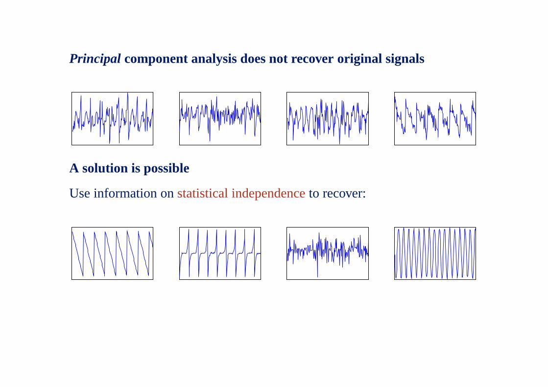
Principal component analysis does not recover original signals

Principal component analysis does not recover original signals

A solution is possible

Use information onstatistical independenceto recover:

Independent Component Analysis(Herault and Jutten, 1984-1991)

• Observed dataxi(t) is modelled using hidden variablessi(t):

xi(t) =m

∑j=1

ai js j(t), i = 1...n (1)

or as a matrix decomposition

X = AS (2)

• Matrix of ai j is constant parameter called “mixing matrix”

• Hidden random factorssi(t) are called “independent components”or “source signals”

• Problem: Estimate bothai j ands j(t), observingonly xi(t)

– Unsupervised, exploratory approach

When can the ICA model be estimated?

• Must assume:

– Thesi are mutually statistically independent

– Thesi arenongaussian (non-normal)

– (Optional:) Number of independent components is equal to number

of observed variables

• Then: mixing matrix and components can be identified (Comon,1994)

A very surprising result!

Background: Principal component analysis and factor analysis

• Basic idea: find directions∑i wixi of maximum variance

• Goal: explain maximum amount of variance with few components

– Noise reduction

– Reduction in computation

– Easier to interpret (?)

– (Vain hope: finds original underlying components)

Why cannot PCA or FA find source signals (original components)?

• They use only covariances cov(xi,x j)

• Due to symmetry cov(xi,x j) = cov(x j,xi), only≈ n2/2 available

• Mixing matrix hasn2 parameters

Why cannot PCA or FA find source signals (original components)?

• They use only covariances cov(xi,x j)

• Due to symmetry cov(xi,x j) = cov(x j,xi), only≈ n2/2 available

• Mixing matrix hasn2 parameters

• So,not enough informationin covariances

– “Factor rotation problem”: Cannot distinguish between

(s1,s2) and (√

2s1+√

2s2 ,√

2s1−√

2s2)

ICA uses nongaussianity to find source signals

• Gaussian (normal) distribution is completely determined by covariances

• But: Nongaussian data has structure beyond covariances

– e.g.E{xix jxkxl} instead of justE{xix j}

• Is it reasonable to assume data is nongaussian?

– Many variables may be gaussian because sum of many independent

variables (central limit theorem), e.g. intelligence

– Fortunately, signals measured by physical sensors are usually quite

nongaussian

Some examples of nongaussianity in signals

0 1 2 3 4 5 6 7 8 9 10−2

−1.5

−1

−0.5

0

0.5

1

1.5

2

0 1 2 3 4 5 6 7 8 9 10−4

−3

−2

−1

0

1

2

3

4

5

0 1 2 3 4 5 6 7 8 9 10−8

−6

−4

−2

0

2

4

6

8

10

−2 −1.5 −1 −0.5 0 0.5 1 1.5 20

0.1

0.2

0.3

0.4

0.5

0.6

0.7

−4 −3 −2 −1 0 1 2 3 4 50

0.1

0.2

0.3

0.4

0.5

0.6

0.7

−8 −6 −4 −2 0 2 4 6 8 100

0.1

0.2

0.3

0.4

0.5

0.6

0.7

Illustration of PCA vs. ICA with nongaussian data

Two components with uniform distributions:

Original components, observed mixtures, PCA, ICA

PCA does not find original coordinates, ICA does!

Illustration of PCA vs. ICA with gaussian data

Original components, observed mixtures, PCA

Distribution after PCA is the same as distribution before mixing!

⇒“Factor rotation problem”

How is nongaussianity used in ICA ?

• Classic Central Limit Theorem:

– Average of many independent random variables will have a

distribution that is close(r) to gaussian

• So, roughly: Any mixture of components will be more gaussianthan

the components themselves

How is nongaussianity used in ICA ?

• Classic Central Limit Theorem:

– Average of many independent random variables will have a

distribution that is close(r) to gaussian

• So, roughly: Any mixture of components will be more gaussianthan

the components themselves

• Maximizing the nongaussianityof ∑i wixi, we can findsi.

• Also known as projection pursuit.

• Cf. principal component analysis: maximize variance of∑i wixi.

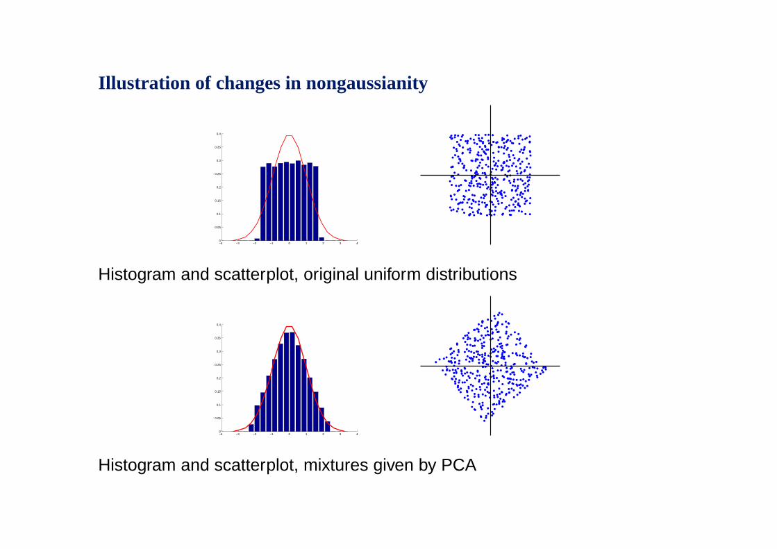
Illustration of changes in nongaussianity

−4 −3 −2 −1 0 1 2 3 40

0.05

0.1

0.15

0.2

0.25

0.3

0.35

0.4

Histogram and scatterplot, original uniform distributions

−4 −3 −2 −1 0 1 2 3 40

0.05

0.1

0.15

0.2

0.25

0.3

0.35

0.4

Histogram and scatterplot, mixtures given by PCA

ICA algorithms consist of two ingredients

1. Nongaussianity measure

• Kurtosis: a classic, but sensitive to outliers.

• Differential entropy: statistically better, but difficultto compute.

• Approximations of entropy: a practical compromise.

2. Optimization algorithm

• Gradient methods: natural gradient, “infomax”

(Bell, Sejnowski, Amari, Cichocki et al 1994-6)

• Fixed-point algorithm: FastICA(Hyvarinen, 1999)

Example of separated components in brain signals (MEG)Temporal envelope (arbitrary units)

1

Fourier amplitude (arbitrary units)

2

3

4

5

6

7

8

100 200 300

9

Time (seconds)5 10 15 20 25 30

Frequency (Hz)

Distribution over channels Phase differences

0

(Hyvarinen, Ramkumar, Parkkonen, Hari, NeuroImage, 2010)

Recent Advance 1: Causal analysis

• A structural equation model (SEM)

analyses causal connections as

xi = ∑j 6=i

bi jx j +ni

• Cannot be estimated in gaussian case

without further assumptions

• Again, nongaussianity solves the prob-

lem (Shimizu et al, 2006)

x1

x2

0.49

x3

0.7

x4

-1.2

x5

0.17

x6

0.0088

-0.14

0.91

0.54 0.97

-0.063

-0.12 -0.42

x7

-0.77

0.87 -0.66

Recent Advance 2: Analysing reliability of components (testing)

• Algorithmic reliability: Are there local minima?

Can be analysed by rerunning from different initial points(a)

• Statistical reliability: Is the result just random/accidental?

Can be analyzed by bootstrap(b)

• Our Icasso package(Himberg et al, 2004)visualizes reliability:

0 2 4 6 8 10−6

−5

−4

−3

−2

−1

0

1a)

0 2 4 6 8 10−6

−5

−4

−3

−2

−1

0

1b)

1

2

3

4

5

6

7

8

9

10

11

12 13

14 15

16

1718

19

20

A B

• New: A proper testing procedure which gives p-values(Hyvarinen, 2011)

Recent Advance 3: Three-way data (“Group ICA”)

• Often ones measures several data matricesXk,k = 1, . . . ,r,e.g. different conditions, measurement sessions, subjects, etc.

• Each matrix could be modelledXk = AkSk

– but how to connect the results?(Calhoun, 2001)

a) If mixing matrices same

for all Xk, use

X1 =(

X1,X2, . . . ,Xr

)

= A(

S1,S2, . . . ,Sr

)

b) If component values same

for all Xk, use

X2 =

X1

...

Xr

=

A1

...

Ar

S

• If both Ak andSk the same: analyse average data matrix, or combineICA with PARAFAC (Beckmann and Smith, 2005).

Recent Advance 4: Dependencies between components

• In fact, estimated components are often not independent

– ICA does not have enough parameters to force independence

• Many authors model correlations of squares, or “simultaneous activity”

Two signals that are uncorrelated but whose squares are correlated.

• On-going work on even linearly correlated components (Sasaki et al,

2011)

• Alternatively, in parallel time series, innovations of VARmodel could

be independent (Gomez-Herrero et al, 2008)

Recent Advance 5: Better estimation of basic linear mixing

• In case of time signals, we can do ICA on time-frequency

decompositions (Pham, 2002; Hyvarinen et al, 2010)

• If the data is by its very nature non-negative, we could impose the same

in the model (Hoyer, 2004)

– Zero must have some special meaning as a baseline

– E.g. Fourier spectra

• More precise modelling of nongaussianity of components could also

improve estimation.

Summary

• ICA is a very simple model: Simplicity implies wide applicability.

• A nongaussian alternative to PCA or factor analysis.

• Finds a linear decomposition by maximizing nongaussianityof thecomponents.

– These (hopefully) correspond to the original sources

• Recent advances:

– Causal analysis, or structural equation modelling, using ICA

– Testing of independent components for statistical significance

– Group ICA, i.e. ICA on three-way data

– Modelling dependencies between components

– Imporovements in estimating the basic linear mixing model

• “Nongaussianity is beautiful” !?