indeterminacy and imperfect information
TRANSCRIPT

Discussion PaperDeutsche BundesbankNo 01/2020
Indeterminacy and imperfect information
Thomas A. Lubik(Federal Reserve Bank of Richmond)
Christian Matthes(Indiana University)
Elmar Mertens(Deutsche Bundesbank)
Discussion Papers represent the authors‘ personal opinions and do notnecessarily reflect the views of the Deutsche Bundesbank or the Eurosystem.

Editorial Board: Daniel Foos Stephan Jank Thomas Kick Malte Knüppel Vivien Lewis Christoph Memmel Panagiota Tzamourani
Deutsche Bundesbank, Wilhelm-Epstein-Straße 14, 60431 Frankfurt am Main, Postfach 10 06 02, 60006 Frankfurt am Main
Tel +49 69 9566-0
Please address all orders in writing to: Deutsche Bundesbank, Press and Public Relations Division, at the above address or via fax +49 69 9566-3077
Internet http://www.bundesbank.de
Reproduction permitted only if source is stated.
ISBN 978–3–95729–660–3 (Printversion) ISBN 978–3–95729–661–0 (Internetversion)

Non-technical summary
Research Question
A regular recommendation for the design of monetary policy is to use rules that respond
strongly to inflation and other economic variables. According to the so-called Taylor
principle, a strong response to inflation is important to avoid multiple equilibria that could
otherwise lead to persistent swings in inflation. However, these prescriptions typically
assume that public and policymakers can perfectly observe the state of the economy.
Instead, we consider the following case of imperfect information: Policymakers receive only
noisy signals, based on which they form estimates of economic conditions, and plug these
estimates into an otherwise standard policy rule. We ask whether the Taylor principle
then still helps to avoid multiple equilibria.
Contribution
We consider an imperfect information case that has been widely used before, but, typically
under the assumption that there was a unique equilibrium. We are the first to document
that there is an inherent risk of multiple equilibria in this case, even when the policy rule
adheres to the Taylor principle.
Results
Multiple equilibria are a generic feature of our setting, since the imperfectly informed pol-
icymaker cannot distinguish shocks to economic fundamentals from self-fulfilling changes
in expectations of the public. A further, novel feature of our environment is that the
variability of these belief shocks is bounded to ensure consistency of expectations between
policymaker and public.

Nichttechnische Zusammenfassung
Fragestellung
Ein regelmaßiger Ratschlag fur die Gestaltung der Geldpolitik besteht darin, Regeln zu
verwenden, die stark auf die Inflation und andere wirtschaftliche Variablen reagieren. Nach
dem sogenannten Taylor-Prinzip ist eine starke Reaktion auf die Inflation wichtig, um mul-
tiple Gleichgewichte zu vermeiden, die andernfalls zu anhaltenden Inflationsschwankungen
fuhren konnten. Diese Vorschlage setzen jedoch voraus, dass Offentlichkeit und politische
Entscheidungstrager die Wirtschaftslage direkt beobachten konnen. Stattdessen betrach-
ten wir den folgenden Fall unvollstandiger Informationen: Die politischen Entscheidungs-
trager empfangen nur ungenaue Signale, auf deren Grundlage sie Schatzungen der wirt-
schaftlichen Bedingungen bilden, und fugen diese Schatzungen in eine standardmassige
Zinsregel ein. Wir fragen, ob in diesem Fall das Taylor-Prinzip ausreicht multiple Gleich-
gewichte zu vermeiden.
Beitrag
Wir betrachten eine Umgebung mit unvollstandiger Information, welche bereits regel-
maßig in der Literatur zur Anwendung gekommen ist, aber typischerweise unter der An-
nahme, dass ein einziges Gleichgewicht vorliegt. Wir sind die ersten, die dokumentieren,
dass in diesem Fall ein inharentes Risiko fur mehrere Gleichgewichte besteht, selbst wenn
die Zinsregel dem Taylor-Prinzip entspricht.
Ergebnisse
Multiple Gleichgewichte sind ein allgemeines Merkmal unserer Modellumgebung, da der
unvollstandig informierte politische Entscheidungstrager Schocks von wirtschaftlichen
Fundamentaldaten nicht von unerwarteten, selbsterfullender Anderungen in den Erwar-
tungen der Offentlichkeit unterscheiden kann. Ein weiteres, neuartiges Merkmal unse-
res Modells ist, dass die Variabilitat dieser Erwartungsschocks zwangslaufig begrenzt ist,
um die Konsistenz der Erwartungen zwischen politischen Entscheidungstragern und der
Offentlichkeit zu gewahrleisten.

Deutsche Bundesbank Discussion Paper No 01/2020
Indeterminacy and Imperfect Information∗
Thomas A. LubikFederal Reserve Bank of Richmond†
Christian MatthesIndiana University‡
Elmar MertensDeutsche Bundesbank§
Abstract
We study equilibrium determination in an environment where two kinds of agentshave different information sets: The fully informed agents know the structure ofthe model and observe histories of all exogenous and endogenous variables. Theless informed agents observe only a strict subset of the full information set. Alltypes of agents form expectations rationally, but agents with limited informationneed to solve a dynamic signal extraction problem to gather information aboutthe variables they do not observe. In this environment, we identify a new channelthat leads to equilibrium indeterminacy: Optimal information processing of theless informed agent introduces stable dynamics into the equation system that leadto self-fulling expectations. For parameter values that imply a unique equilibriumunder full information, the limited information rational expectations equilibrium isindeterminate. We illustrate our framework with a monetary policy problem wherean imperfectly informed central bank follows an interest rate rule.
Keywords: Limited information; rational expectations; signal extraction; beliefshocks
JEL classification: C11, C32, E52.
∗The views expressed in this paper are those of the authors and should not be interpreted as thoseof the Federal Reserve Bank of Richmond, the Federal Reserve System, the Deutsche Bundesbank, orthe Eurosystem. This paper is accompanied by a Supplementary Appendix, that is available from theauthors upon request.
†Federal Reserve Bank of Richmond, Research Department, P.O. Box 27622, Richmond, VA 23261.Tel.: +1-804-697-8246. Email: [email protected].
‡Indiana University, Department of Economics, Wylie Hall 202, Bloomington, IN 47405. Email:[email protected].
§Deutsche Bundesbank, Research Centre, Wilhelm-Epstein-Strasse 14, 60431 Frankfurt am Main,Germany. Email: [email protected].
1 Introduction
Asymmetric information is a pervasive feature of economic environments. Even whenagents are fully rational, their expectation formation and decision-making process areconstrained by the fact that information may be imperfectly distributed in the economy forreasons such as costs of information acquisition. Asymmetric information is also a centralissue for the conduct of monetary policy as policymakers regularly face uncertainty aboutthe true state of the economy, either because they are uncertain about the structure of theeconomy or because they receive data in real time that are subject to measurement error.In environments where information is perfect and symmetrically shared, the literaturehas shown that ill-designed policy rules can cause indeterminacy. We study equilibriumdeterminacy in an asymmetric information setting, where policy is conducted based onestimates of the true state of the economy.
We consider an economic environment with two types of agents, one who has full in-formation about the state of economy while the other agent is imperfectly informed. Morespecifically, the less informed agent’s information set is nested within the fully informedagent’s. We think of the two agents as a fully informed public, or alternatively, the privatesector as a data-generating process for aggregate outcomes, and a less informed policy-maker. We model the private sector as a homogeneously informed representative agentwho is perfectly informed about the aggregate state whereas the policymaker operatesunder imperfect imperfection, which, for instance, can take the form of aggregate datasubject to measurement error.1
A key assumption of our modelling framework is that both types of agents, the pol-icymaker and the private sector, form rational expectations, but based on different in-formation sets. Private-sector behavior is characterized by a set of linear, expectationaldifference equations. On the other hand, the policymaker’s behavior is characterizedby the use of a policy instrument. It is set according to a rule that responds to thepolicymaker’s optimal estimates of economic conditions.2 Formally, we consider linear,stochastic equilibria with time-invariant decision rules and Gaussian shocks. In this case,the rational inference efforts of the policymaker are represented by a dynamic signal ex-traction problem as captured by the Kalman filter. The interaction of the two sets ofexpectation formation processes represents the fundamental mechanism underlying equi-librium determination.
The central result of our paper is that equilibrium indeterminacy is generic in thisimperfect information environment for a broad class of linear models that have uniqueequilibria under full information. Optimal information processing of the less informedagent introduces additional stable dynamics into the equation system that then lead toself-fulling expectations. Intuitively, the interaction of the two expectation processes gen-erates an endogenous feedback mechanism in a similar vein to strategic complementaritiesor the application of ad-hoc behavior in the standard indeterminacy literature. Moreover,the interplay of expectations based on different information sets results in equilibrium
1Such a dichotomy is well-established in the learning literature. Where our work differs is that bothagents have rational expectations and know the structure of the economy, although not necessarily itsstate.
2As a specific example, we consider a Taylor-type interest-rate rule that responds to the policymaker’sprojection of inflation.
1

outcomes that are not certainty equivalent even though we only consider environmentsthat are linear. While the rationality of expectations under both information sets placesnon-trivial restrictions on outcomes, they are not sufficient to rule out multiple equilibria.
We characterize the outcomes of different equilibria as the result of non-fundamentaldisturbances, similar to the perfect-information literature on equilibrium determinacy inlinear rational expectations models. Such belief shocks are unrelated to fundamentalshocks in the original economic setup and can be interpreted as self-fulfilling shifts inexpectations, or beliefs, that cause fluctuations consistent with the concept of a linear,stationary equilibrium. When there is indeterminacy in the perfect-information case,there are no restrictions on the scale of effects caused by belief shocks. In contrast,the potential effects of belief shocks are tightly bounded in our imperfect informationenvironment. The bounds arise from the required consistency of expectations of thepublic and the policymaker and the assumption that we consider only environments thathave a unique equilibrium under full information.
Our main application is a standard New Keynesian model where monetary policy fol-lows a Taylor-type interest-rate rule. The rule coefficients satisfy the Taylor principle,which assures determinacy under full information. Under imperfect information, how-ever, the central bank cannot adjust the nominal rate directly in response to movementsin actual inflation and the output gap. Instead, policymakers observe noisy signals ofinflation and output and the policy rate responds to optimal projections of inflation andoutput gap. The sensitivity of the policy rate to movements in actual inflation and theoutput gap then depend on the sensitivity of policymakers’ projections to the incomingsignals. The more the central bank is successful at stabilizing inflation and output gap,the noisier will be the signal and policymakers’ projections will barely respond. As aresult, the policy rate will not respond much to actual inflation and the output gap, andthe Taylor principle effectively ceases to hold.
Likewise, indeterminacy cannot lead to non-fundamental shocks becoming an arbitrar-ily large driver of inflation and the output gap. Otherwise, the central bank’s signal wouldbecome highly informative and the policy rate would respond with sufficient strength toactual inflation and the output gap to re-establish determinacy. In sum, while we findgeneric indeterminacy in this setting, the extent to which indeterminacy manifests itselfis bounded. The variance bound on indeterminacy-induced fluctuations is a novel andimportant result of our setup. This bound arises when the central bank observes noisysignals of endogenous, variables and it reflects the endogenous response of the signals’information content to monetary policy. Key features of our analysis are also illustratedwith a simple Fisher-equation model.
Our paper touches upon three strands in the literature. First, our paper contributes tothe burgeoning literature on imperfect information in macroeconomic models. An impor-tant topic of the existing literature have been the implications of dispersed informationamong different members of the public and the resulting effects on their strategic interac-tions and the informational value of prices. Key contributions by Nimark (2008a, 2008b,2014), Angeletos and La’O (2013), and Acharya, Benhabib and Huo (2017) demonstratethat imperfect information has important implications for the amplification and propa-gation of economic shocks. However, while the literature has been aware of the potentialfor multiple equilibria, this has usually not been a key issue of the analysis. In that vein,our paper is much closer to Benhabib, Wang and Wen (2015) who consider sentiment
2

shocks in their New Keynesian model with imperfect information in the private sector.In contrast to our setup, which involves the interaction between a policymaker and thepublic under different information sets, sunspot or belief shocks do not arise endogenouslyin their setting. In that respect, our framework is closer to Rondina and Walker (2017).
A number of papers have also analyzed the effects of policy actions on the informationalvalue of market signals and their interplay when policy itself responds to market infor-mation (Goodhart 1987, Bernanke and Woodford 1997, Morris and Shin 2018, Siemroth2019). This literature has typically found a tension between a policymaker’s desire to ex-tract information from prices as policy seeks to influence market outcomes. In our setup,the degree to which indeterminacy gives rise to fluctuations driven by non-fundamentalshocks depends on the outcomes targeted by policy. What is unique in our analysis, is theinterplay between noisy signals gleaned from endogenous variables and indeterminacy.3
Second, our research also makes a contribution to the literature on indeterminacy inlinear rational expectations models by expanding the set of plausible economic mecha-nisms that can lead to multiple equilibria. A key element of the indeterminacy literatureis the presence of a mechanism that validates self-fulfilling expectations. In the standardliterature, these could arise from what is often termed strategic complementarities, such asincreasing returns to scale in production that are not internalized, as in the seminal con-tributions of Benhabib and Farmer (1994), Farmer and Guo (1994), and Schmitt-Grohe(1997). An alternative mechanism is the interplay between economic agents’ forward-looking behavior and the reaction function of a policymaker, which Clarida, Gali andGertler (2000) and Lubik and Schorfheide (2004) show to be a key feature of macroeco-nomic fluctuations.4
In contrast, our framework does not rely on these previously identified sources of in-determinacy but rather on the interaction of different expectation formation processesunder asymmetric information sets. This also sets our framework apart from the generalimperfect information literature, which is largely concerned with the strategic interac-tion between agents in the private sector. Although our framework utilizes the formal-ism of the indeterminacy literature, where we build on the contributions of Lubik andSchorfheide (2003, 2004) and Farmer, Khramov and Nicolo (2015), the mechanism to getthere is novel. More specifically, we show that in an imperfect information environmentthe standard root-counting approach in the literature is inadequate in identifying the setof multiple equilibria. At the same time, we show that the set of multiple equilibria,despite the generic pervasiveness of indeterminacy, is tightly circumscribed by internalconsistency requirements for the interaction between the two expectation processes. Ourpaper thereby puts some caveats on the notion that sunspot shocks are unrestricted intheir effects on macroeconomic outcomes.
Third, the applications in our paper speak to the monetary policy literature concernedwith the effects of interest-rate rules on determinacy. A well-known result from this litera-ture is the Taylor principle, which requires that interest rate rules respond to endogenous
3Bernanke and Woodford (1997) consider implications for existence and determinacy of equilibriaarising from an inflation-targeting central bank’s use of private-sector forecasts in lieu of its own. A keydifference of our work are the consequences for determinacy arising from the explicit consideration of animperfectly informed central bank’s signal extraction problem.
4Ascari, Bonomolo and Lopes (2019) also point to sunspot-driven equilibria as a key source of fluctu-ations during the high-inflation era of the 1970s.
3

variables with sufficient strength, to avoid multiple equilibria and ensure determinacy.Clarida et al. (2000) and Lubik and Schorfheide (2004) have pointed to a neglect of theTaylor rule as a possible factor behind the Great Inflation. However, their evidence isbased on a full-information perspective that does not account for the uncertainties facedby the Federal Reserve in assessing the state of the economy in real time, as discussed byOrphanides (2001). The framework that we develop in this paper sheds new light on thisissue.
A key paper in this literature is Orphanides (2003) who models the consequences of animperfectly informed central bank for economic outcomes. Similar to our framework, hismodel considers a policy rule that responds to estimates of economic conditions generatedfrom optimal signal extraction efforts. But in a fundamental difference to our framework,his model is purely backward-looking so that the issue of indeterminacy does not arise.Our paper also relates to Svensson and Woodford (2004) and Aoki (2006) who deriveconditions for optimal policy when the policymaker is less informed than the public inforward-looking linear rational expectations models, but take determinacy as given.5
This paper is structured as follows: The next section introduces our framework bymeans of a simple example in which we can derive analytical results. The section pro-ceeds by developing the various model components sequentially so as to build up thefull set of equilibrium relationships. We also discuss various extensions and some addi-tional findings that connect our framework to the literature. Section 3 contains the mainbody of the paper. We present a general linear rational expectations framework with het-erogeneous information sets and use results from general linear systems theory to proveexistence of a variety of equilibria. It is here that we establish our central result thatequilibrium indeterminacy is generic in this framework. We conduct some quantitativeexercises in section 4. We first solve the simple example of section 2 numerically in orderto provide additional insights. In the next step, we solve a New Keynesian model underour informational assumptions. We show that while indeterminacy is, in fact, genericin this policy-relevant model, the quantitative implications appear relatively limited. Insection 5, we consider a set of alternative policy rules that lead to determinate outcomes.Section 6 concludes and discusses further extensions of our framework.
2 A Simple Example Model
We develop the basic concepts and ideas underlying our modelling framework by means ofa simple example. First, we describe the basic structural relationships before introducingtwo types of information sets. For exposition purposes we distinguish information setswhere the observed signals reflect solely exogenous variables or where the signal alsoreflects endogenous variables. We then introduce the key component of the framework,namely optimal information extraction by the less informed agent via Kalman-filtering,and a projection condition that rational expectations equilibria in our framework need to
5Applications following Svensson and Woodford to various economic issues are Carboni and Ellison(2011), Dotsey and Hornstein (2003), and Nimark (2008b). Evans and Honkapohja (2001) and Or-phanides and Williams (2006, 2007) revisit the question of policymaking under imperfect information inan environment with learning. Faust and Svensson (2002) and Mertens (2016) study the implications foroptimal policy of the opposite informational asymmetry, where the public does not perfectly share thepolicymaker’s information set.
4

obey. We conclude this section by discussing the underlying intuition and some specialresults from the simple framework.
2.1 Economic Framework
We consider a simple textbook model of inflation determination in a frictionless economy.The economy is described by a Fisher equation that links the nominal interest rate itto the real rate rt via expected inflation Etπt+1, where Et is an expectation operator.The nominal rate is set according to a monetary policy rule where it responds to currentinflation πt.
6 Reflecting the central role of the Fisher equation here, we refer to the smallmodel also as a Fisher economy. We assume that the real rate is characterized by anexogenous AR(1) process with a Gaussian shock. The equation system is thus given by:
it = rt + Etπt+1, (1)
it = φπt, (2)
rt = ρrt−1 + εt, (3)
where εt ∼ iid N(0, σ2ε) and |ρ| < 1. Throughout this paper we assume that the monetary
policy parameter φ is outside the unit circle, |φ| > 1.There are two agents in this economy: a representative private-sector agent whose
behavior is characterized by the Fisher equation (1), and a central bank whose behavioris given by a monetary policy rule such as (2). We assume that the agents know thestructure of the economy, including the structural parameters, and that they observe thehistory of their respective information sets. Crucially, both agents form expectationsrationally. The central assumption of our framework is that the two agents have different,but nested information sets. The full information set St contains realizations of all shocksthrough time t, where Et is the rational expectations operator under full information,so that for some variable xt, Etxt+h = E (xt+h|St), for all h, and Etxt = xt. We alsodefine a limited information set Zt which is nested in St, Zt ⊂ St.7 The expectations, orprojections, of the less informed agent for any variable xt are denoted as xt|t = E (xt|Zt)and xt+h|t = E (xt+h|Zt). Since Zt is spanned by St we can apply the law of iteratedexpectations to obtain: E (E(xt+h|Zt)|St) = xt+h|t.
We consider two informational environments: full and limited information. Under fullinformation rational expectations (FIRE), both agents are assumed to know St.8 Thismeans that they observe all variables in the model without error, that they know thehistory of all shocks, and that they understand the structure of the economy and thesolution concepts. Under limited information rational expectations (LIRE), we assumethat one agent has access to the full information set St, while the other observes thelimited information set Zt only. For the purposes of this simple example, we assume thatthe private sector is fully informed whereas the central bank has limited information.
6In the Supplementary Appendix, we also consider a policy rule of the type: it = rt + φπt, with atime-varying intercept given by the real rate of interest.
7Allowing Zt to be only weakly nested in St, Zt ⊆ St, would also encompass the case when bothagents are fully informed. We will typically consider the limited-information case as such that Zt isstrictly less informative than St.
8In terms of notation, the full-information case corresponds to the situation where Zt = St.
5

2.2 Rational Expectations Equilibria with Full Information
The equation system (1) - (3) forms a linear rational expectations model that can besolved under FIRE with standard methods. Substituting the policy rule into the Fisherequation yields a relationship in inflation with driving process rt:
φπt = Etπt+1 + rt. (4)
The type of solution depends on the value of the policy coefficient φ. It is well knownthat the solution is unique if and only if |φ| > 1. In this case, the determinate rationalexpectations (RE) solution is: πt = 1
φ−ρrt and it = φφ−ρrt. Inflation and the nominal rate
inherit the properties of the exogenous process rt and are thus first-order autoregressiveprocesses.
When |φ| < 1, the full-information solution is indeterminate, and there are infinitelymany solutions to equation (4). Although the remainder of the paper considers thecase |φ| > 1, it is instructive to review the implications of equilibrium indeterminacywhen φ is inside the unit circle, since we utilize these concepts later. We follow theapproach developed by Lubik and Schorfheide (2003), which extends the Sims (2002)solution method to the case of indeterminacy.
We define the rational expectations forecast error ηt = πt−Et−1πt, whereby Et−1ηt = 0by construction. This allows us to substitute out inflation expectations Etπt+1 in (4), sothat we can write:
πt = φπt−1 + rt−1 + ηt. (5)
It is easily verifiable that this representation is a solution to the expectational differenceequation (4). Inflation is a stationary process with autoregressive parameter |φ| < 1 anddriving process rt−1. What makes this equilibrium indeterminate is the fact that thesolution imposes no restriction on the evolution of ηt other than that it is a martingaledifference sequence with Et−1ηt = 0. Consequently, there can be infinitely many solutions.
Without loss of generality, we can, however, put some structure on the solution.9
Following Farmer, Khramov, and Nicolo (2015) we decompose the RE forecast error ηtinto a fundamental component, namely the policy innovation εt, and a non-fundamentalcomponent, the belief shock bt. More specifically, we can write ηt = γεεt + γbbt, whereEt−1bt = 0.10 The loadings −∞ < γε, γb < ∞ on the two sources of uncertainty areunrestricted and their choice is arbitrary. They can be used to index specific equilibriawithin the set of indeterminate equilibria. A specific solution to (4) when |φ| < 1 cantherefore be written as:
πt = φπt−1 + rt−1 + γεεt + γbbt. (6)
Returning to the case of |φ| > 1, we can also compute an RE equilibrium for thecase when the dynamic system is conditioned down onto the information set Zt. Since
9Strictly speaking, this is without loss of generality within the set of equilibria that are time-invariantand linear. There are other non-linear equilibria that can be constructed in this linear model. See Evansand McGough (2005) for further discussion.
10The interpretation of a belief shock in the terminology of Lubik and Schorfheide (2003) and Farmer,Khramov, and Nicolo (2015) emerges when the inflation equation is rewritten in terms of expectationsonly. Define ξt = Etπt+1 and rewrite equation (4) as ξt = φξt−1 + rt + φηt. In this representation, theforecast error ηt is akin to an innovation to the conditional expectation ξt.
6

the content of this information set is known to both agents, we can apply the law ofiterated expectations: E (E(xt+h|Zt)|St) = xt+h|t. Except for changing the informationset on which the expectations operator is conditioned, the structure of the system remainsunchanged. The policy rule now becomes:
it|t = φπt|t. (7)
Following the same steps as before, we find that:
πt+1|t = φπt|t + rt|t, (8)
which is a first-order difference equation in projected inflation πt|t. Under the maintained
assumption that |φ| > 1, the RE equilibrium is πt|t = 1φ−ρrt|t and it|t = φ
φ−ρrt|t. Theform of the solution is isomorphic to the FIRE solution above. That is, central bankprojections of inflation and the evolution of the policy rate obey the same functional formas the actual variables in the full information model. Moreover, in our setup central bankdecisions are always based on Zt such that it = it|t. The key insight is that under Zt, thecentral bank has less information than under St, but it still forms expectations rationallyunder its own information set, given its real rate projections rt|t.
11
2.3 Rational Expectations Equilibria with Limited Information
The key aspect of our limited information framework is that there are two expectationformation processes interacting with each other. The nature of this interaction, and how itaffects equilibrium determination, depends on how the limited-information agent extractsand updates information. Our framework has four building blocks: first, the relation-ships describing the fully-informed agent; second, those of the limited-information agent;third, the filtering and updating mechanism used by the latter to gain additional informa-tion; and fourth, restrictions on agents’ projections to ensure consistency of expectationformation in an RE equilibrium.
In the simple example considered thus far, the first element is given by the Fisherequation (1) and the law of motion of the real rate (3). Considering the second buildingblock, we assume that the central bank is the less informed agent and therefore has accessto the information set Zt. As in Svensson and Woodford (2004), policy is set based ontarget variable projections. Specifically, the behavior of the central bank is given by alimited information policy rule where the policy rate responds to the inflation projectionπt|t:
it = φπt|t (9)
The third element is the specification of the central bank’s information extraction andupdating problem. The policymaker is aware of the limited information set and solves asignal extraction problem to conduct inference about unobserved variables.12 The model
11This is a key difference to the framework in Lubik and Matthes (2016) who assume that the centralbank engages in least-squares learning to gain information about private-sector outcomes. In our setup,the deviation from the standard RE benchmark is only minor in the sense that the central bank does notobserve everything that the private sector does, but employs fully rational expectations in its inferencesabout current and future conditions.
12Conceptually, this is an environment where the central bank receives noisy measurements of incoming
7

is linear and the exogenous shocks are Gaussian; in addition, we assume that the beliefshocks are Gaussian. Without loss of generality, the variance of belief shocks is normalizedto one:13
bt ∼ N(0, 1). (10)
As a result, the Kalman filter is the optimal filter in this environment. The gain in the op-timal projection equation is endogenous and depends on the second moments of the modelvariables in an equilibrium. In turn, existence and uniqueness of an equilibrium dependson the endogenous Kalman gain. This feature of our framework implies a non-trivialfixed-point problem. Finally, the fourth building block of our framework is an additionalrestriction on equilibrium determination. We posit that rational expectations formationacross all information sets has to be mutually and internally consistent. Specifically, thecentral bank’s behavior is constrained by its own projections, namely πt|t = 1
φ−ρrt|t and
it = φφ−ρrt|t, and a projection for rt|t. These projections imply a restriction on the joint
behavior of the model variables’ second moments so as to validate the RE of the fullyinformed and the limited-information agents.
We now discuss the solution of our simple framework in two steps. We specify simpleinformation sets that make the central bank’s projection equations analytically tractable,whereby we distinguish between exogenous and endogenous information sets. The for-mer contains only exogenous variables where there is no feedback between projection andmodel evolution. Specifically, we assume that the central bank receives a noisy measure-ment of the real rate of interest. In the second step, we assume endogenous informationwhere the central bank observes inflation with a measurement error.
2.3.1 Equilibrium with an Exogenous Signal
We assume that the central bank observes the real rate with measurement error νt ∼iid N(0, σ2
ν), so that its information set is Zt = Zt, Zt−1, . . ., with Zt = rt + νt.14 The
signal Zt is exogenous in that the real rate is an exogenous process that does not dependon other endogenous variables.15 The Kalman projection equation for the real rate is:
rt|t = rt|t−1 + κr(rt − rt|t−1 + νt
), (11)
where the Kalman gain κr is an endogenous coefficient, and the one-step-ahead projectionof the real rate is rt|t−1 = ρrt−1|t−1.
We now combine the private sector Fisher equation (1) with the policy rule (9):
φπt|t = rt + Etπt+1. (12)
data but makes decisions in real time based on its best projections of the true underlying data.13Similar to the full-information case shown in (6), belief shocks will enter the system only via the
endogenous forecast error, which linearly depends on the belief shock bt with sensitivity γb, This allowsus to normalize the variance of belief shocks.
14In addition, the central bank knows the structure of the economy and all parameters of the model,which are common knowledge. For brevity, these elements of the information set are omitted in ournotation.
15However, the process of making projections of the real rate, that is, of gaining information about itstrue value can depend on endogenous outcomes.
8

The evolution of inflation depends on two expectation processes: the central bank’s pro-jection of inflation πt|t and the private sector’s expectation Etπt+1. Using the formalismdescribed above, we introduce the RE forecast error ηt and rewrite this equation as:
πt = φπt−1|t−1 − rt−1 + ηt. (13)
In addition, recall that after conditioning down all equations of the model onto Zt andsolving for an RE equilibrium conditional on Zt, we obtain:
πt|t =1
φ− ρrt|t . (14)
Equation (14) is a consistency condition for the RE equilibrium that we will also refer toas “projection condition” since it restricts central bank projections to be consistent withpredictions from the full-information model.
We can now combine these equations into a linear RE system:
πt =φ
φ− ρrt−1|t−1 − rt−1 + ηt,
rt|t = (1− κr) ρrt−1|t−1 + κrρrt−1 + κrεt + κrνt, (15)
rt = ρrt−1 + εt.
The first equation in (15) is derived from the Fisher equation, where we substituted outthe central bank’s lagged inflation projection by using the projection condition (14). Thesecond equation is derived from the Kalman projection equation for the real rate, whilethe third equation is the law of motion of the actual real rate. The set of equationsin (15) is a well-specified equation system in three unknowns: inflation πt, the exogenousreal rate rt, and the central bank projection of the real rate rt|t. In principle, it can besolved using standard methods for linear RE models that allow for indeterminacy suchas Lubik and Schorfheide (2003). However, there are two key differences to the standardframework. First, the gain coefficient κr is endogenous and has to be computed from thesecond moments of the model solution. The second difference is that the central bank’sprojection rt|t has to be consistent with the solution of the full system it determines. Thisprojection condition necessitates an additional computational step in the solution of themodel.
We solve the model in three steps. First, in the exogenous signal case, the Kalman fil-tering problem can be solved independently of the solution for inflation dynamics. Second,as shown below, the Kalman gain lies between zero and one. As a result, rt|t is station-ary and standard root-counting implies that the system (15) is indeterminate. Third,we impose the projection condition. Following Farmer, Khramov, and Nicolo (2015), wefind it convenient to express the endogenous forecast error as a linear combination offundamental and belief shocks:16
ηt = γεεt + γννt + γbbt. (16)
The solution is determinate if γb = 0 and γε and γν are uniquely determined. An RE
16Alongside εt, we refer to the measurement error νt as a fundamental shock, too.
9

equilibrium may not exist when there are no loadings that fulfill the restrictions imposedby and on the model, specifically, the projection condition (14).
We find it convenient to define innovations of any variable xt as its unexpected compo-nent relative to the limited information set Zt−1: xt = xt − xt|t−1, that is, the projectioninnovations. We can then define the projection error variance Σ = var
(rt − rt|t
)=
var (rt) − var(rt|t), whereby cov(rt, rt|t) = var(rt|t). The steady-state Kalman gain is
given by:
κr =cov(rt, Zt
)var(Zt)
, (17)
where Zt = rt + νt. It is straightforward to verify that var (rt) = ρ2Σ + σ2ε and that
var(Zt) = var (rt) + σ2ν . Similarly, we have that cov(rt, Zt) = var (rt). This leads to the
following expression:
κr =ρ2Σ + σ2
ε
ρ2Σ + σ2ε + σ2
ν
, (18)
whereby clearly 0 < κr < 1. We can now find an expression for the projection error
variance Σ by noting that cov(rt, rt|t) = var(rt|t) and var(rt|t)
= κr cov(rt, Zt
), given
the projection equation rt|t = κrZt. Substituting these expressions into the definition ofΣ results in a quadratic equation, commonly known as a Riccati equation:
Σ =ρ2Σ + σ2
ε
ρ2Σ + σ2ε + σ2
ν
σ2ν . (19)
The (positive) solution to this equation is given by:
Σ =1
2ρ2
[−(σ2ε +
(1− ρ2
)σ2ν
)+
√(σ2
ε + (1− ρ2)σ2ν)
2 + 4σ2εσ
2νρ
2
]. (20)
We can now establish that the LIRE model with an exogenous signal vector alwayshas multiple equilibria. We have 0 < κr < 1, from which it follows that |(1− κr) ρ| < 1,so that the law of motion for rt|t in the full equation system is a stable difference equation.In (13), inflation depends only on lags of the real rate rt and lags of the real-rate projectionrt|t, which are both stationary. Without any dependence of inflation on lags of its own,inflation is stationary for any specification of ηt, and we can conclude that the equilibriumcannot be determinate. That is, the structure of the model does not impose restrictionsthat would uniquely pin down the endogenous forecast error ηt and which would typicallyderive from the set of explosive roots in the system. One such restriction could be |κr| > 1,which we can rule out in this case. In other words, the representation (15) is already acandidate solution to the model.
In the final step, we need to ensure that central bank projections for inflation andthe real rate are mutually consistent. Specifically, πt|t = 1
φ−ρrt|t needs to hold along anyequilibrium path. This projection condition imposes a second-moment restriction on inno-
vations with respect to the central bank’s information set cov(πt, Zt
)= 1
φ−ρcov(rt, Zt
).
Since cov(rt, Zt
)= ρ2Σ +σ2
ε , we can write cov(πt, Zt
)= cov (πt, rt) + cov (πt, νt). Using
10

the innovation representation of the projection equation for πt, we have:
πt = −(rt−1 − rt−1|t−1
)+ ηt, (21)
where after some substitution we find that cov (πt, rt) = −ρΣ + γεσ2ε . Similarly, we
have that cov (πt, νt) = γνσ2ν . Combining all expressions results in the following linear
restriction on the shock loadings of the forecast error ηt = γεεt + γbbt + γννt:
γν =φ
φ− ρΣ
σ2ν
+1
φ− ρσ2ε
σ2ν
− σ2ε
σ2ν
γε. (22)
This condition places a linear restriction on γε and γν to guarantee that central bankprojections for inflation and the real rate co-vary as they would in the full informationcase. However, this projection condition does not uniquely determine γε and γν . Moreover,γb is left unrestricted. We can now summarize the solution in the following proposition.
Proposition 1 (LIRE Equilibrium in the Fisher Economy with Exogenous Signal). Theset of stationary RE equilibria in the model (15) under LIRE with exogenous signal Zt =rt + νt is characterized by:
πt =φ
φ− ρrt−1|t−1 − rt−1 + γεεt + γννt + γbbt, (23)
rt|t = (1− κr) ρrt−1|t−1 + κrρrt−1 + κrεt + κrνt, (24)
rt = ρrt−1 + εt, (25)
where:
κr =ρ2Σ + σ2
ε
ρ2Σ + σ2ε + σ2
ν
, (26)
Σ =1
2ρ2
[−(σ2ε +
(1− ρ2
)σ2ν
)+
√(σ2
ε + (1− ρ2)σ2ν)
2 + 4σ2εσ
2νρ
2
], (27)
−∞ < γb <∞,−∞ < γε <∞, γν =φ
φ− ρΣ
σ2ν
+
(1
φ− ρ− γε
)σ2ε
σ2ν
. (28)
Proof. The result follows directly from the positive solution to the Riccati equation (19)and (20) as well as the projection condition (22).
We can draw the following conclusion at this point. Equilibrium indeterminacy isgeneric in this setting in that the endogenous forecast error is not uniquely determinedand that any stationary RE equilibrium allows for the presence of sunspot shocks. Me-chanically, the optimal filter employed by the central bank introduces a stable root intothe system, associated with the Kalman gain κr, and thereby leaves the endogenous fore-cast error undetermined. Although policy obeys the Taylor principle with |φ| > 1, andthere is a unique mapping from central bank projections to endogenous outcomes, equi-librium is generically indeterminate in the full model, in particular, the component thatis orthogonal to the central bank’s information set.17
17By the logic of the root-counting approach to solving linear RE models, the system needs an ‘unstable’
11
A second observation is that the projection condition imposes restrictions on the set ofmultiple equilibria which stands in contrast to the typical indeterminacy case under fullinformation. Optimal filtering restricts how private agents coordinate on an equilibrium,that is, which equilibrium is admissible and consistent with central bank projections.Although the effects of belief shocks with exogenous information are still unrestricted,the relationship between the fundamental real-rate shock and the measurement error issubject to a second moment restriction on their comovement.18 However, this simpleexample is restrictive in that the central bank only observes an exogenous process witherror. In the next step, we therefore analyze an endogenous signal which creates additionalfeedback within the model.
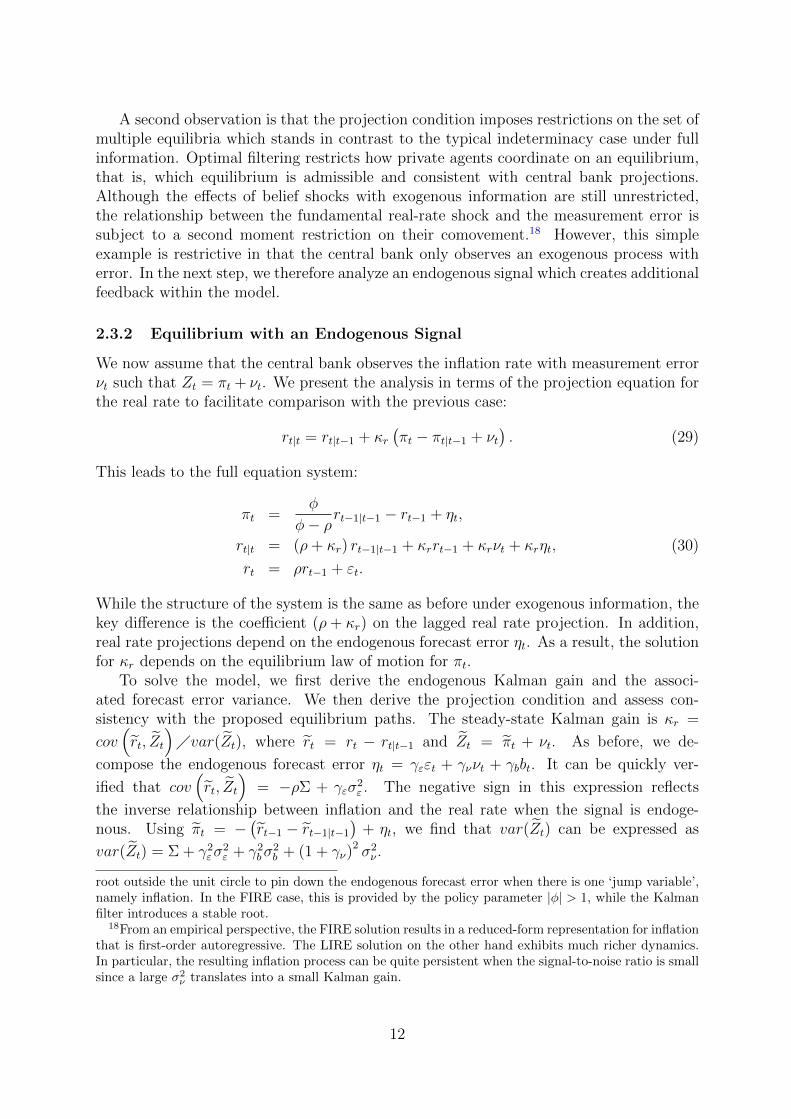
2.3.2 Equilibrium with an Endogenous Signal
We now assume that the central bank observes the inflation rate with measurement errorνt such that Zt = πt + νt. We present the analysis in terms of the projection equation forthe real rate to facilitate comparison with the previous case:
rt|t = rt|t−1 + κr(πt − πt|t−1 + νt
). (29)
This leads to the full equation system:
πt =φ
φ− ρrt−1|t−1 − rt−1 + ηt,
rt|t = (ρ+ κr) rt−1|t−1 + κrrt−1 + κrνt + κrηt, (30)
rt = ρrt−1 + εt.
While the structure of the system is the same as before under exogenous information, thekey difference is the coefficient (ρ+ κr) on the lagged real rate projection. In addition,real rate projections depend on the endogenous forecast error ηt. As a result, the solutionfor κr depends on the equilibrium law of motion for πt.
To solve the model, we first derive the endogenous Kalman gain and the associ-ated forecast error variance. We then derive the projection condition and assess con-sistency with the proposed equilibrium paths. The steady-state Kalman gain is κr =
cov(rt, Zt
)var(Zt), where rt = rt − rt|t−1 and Zt = πt + νt. As before, we de-
compose the endogenous forecast error ηt = γεεt + γννt + γbbt. It can be quickly ver-
ified that cov(rt, Zt
)= −ρΣ + γεσ
2ε . The negative sign in this expression reflects
the inverse relationship between inflation and the real rate when the signal is endoge-nous. Using πt = −
(rt−1 − rt−1|t−1
)+ ηt, we find that var(Zt) can be expressed as
var(Zt) = Σ + γ2εσ2ε + γ2bσ
2b + (1 + γν)
2 σ2ν .
root outside the unit circle to pin down the endogenous forecast error when there is one ‘jump variable’,namely inflation. In the FIRE case, this is provided by the policy parameter |φ| > 1, while the Kalmanfilter introduces a stable root.
18From an empirical perspective, the FIRE solution results in a reduced-form representation for inflationthat is first-order autoregressive. The LIRE solution on the other hand exhibits much richer dynamics.In particular, the resulting inflation process can be quite persistent when the signal-to-noise ratio is smallsince a large σ2
ν translates into a small Kalman gain.
12

We can now derive the following expression for the Kalman gain:
κr =−ρΣ + γεσ
2ε
Σ + γ2εσ2ε + γ2bσ
2b + (1 + γν)
2 σ2ν
. (31)
Although the forecast error variance Σ still needs to be determined as a function of thestructural parameters, we can make two observations already. First, in contrast with theexogenous signal case the gain κr can be negative for small enough γε, that is, κr < 0 ifγε < ρΣ/σ2
ε . Second, existence of a steady-state Kalman filter implies that |ρ + κr| < 1as long as Σ > 0, as shown in Proposition 2 below. We return to a discussion of thecase where rt = rt|t, so that Σ = 0, later in this section. In the next step, we computethe projection error variance Σ = var (rt) − var
(rt|t). Using var (rt) = ρ2Σ + σ2
ε and
var(rt|t)
= κrcov(rt, Zt
)we can derive the following Riccati equation, which is quadratic
in Σ:
Σ = ρ2Σ + σ2ε −
(−ρΣ + γεσ2ε)
2
Σ + γ2εσ2ε + γ2bσ
2b + (1 + γν)
2 σ2ν
. (32)
Finally, an equilibrium has to obey the restrictions imposed by central bank projec-tions, namely πt|t = 1
φ−ρrt|t. This implies a covariance restriction of projection errors whichdiffers from the exogenous signal case because of different information sets. Specifically,
we have that cov(πt, Zt
)= 1
φ−ρcov(rt, Zt
)or alternatively (φ− ρ) cov (πt, πt + νt) =
cov (rt, πt + νt). After some rearranging we can write this expression as:
γν (1 + γν) = − φ
φ− ρΣ
σ2ν
− γ2bφ− ρ
σ2b
σ2ν
+[1− (φ− ρ) γε] γε
φ− ρσ2ε
σ2ν
. (33)
The condition places a quadratic restriction on all three innovation loadings γ in contrastto the linear restriction on γε and γn and unrestricted γb in the exogenous signal case.This can imply that there are no or multiple solution to this equation, and thus for theoverall equilibrium, for a given parameterization of the model. We summarize our findingsin the following proposition.
Proposition 2 (LIRE Equilibrium in the Fisher Economy with Endogenous Signal).The set of stationary RE equilibria in the model (30) under LIRE with endogenous signalZt = πt + νt is characterized by the following dynamic equations:
πt =φ
φ− ρrt−1|t−1 − rt−1 + γεεt + γννt + γbbt, (34)
rt|t = (ρ+ κr) rt−1|t−1 − κrrt−1 + κrγεεt + κr (1 + γν) νt + κrγbbt, (35)
rt = ρrt−1 + εt,
13

With Σ > 0, we have:
|ρ+ κr| < 1 (36)
Σ =1
2
(α +
√α2 + 4β
), (37)
α = (1 + 2ργε)σ2ε − (1− ρ)2
(γ2εσ
2ε + γ2b + (1 + γν)
2 σ2ν
), (38)
β =(γ2b + (1 + γν)
2 σ2ν
)σ2ε , (39)
κr =−ρΣ + γεσ
2ε
Σ + γ2εσ2ε + γ2b + (1 + γν)
2 σ2ν
, (31)
γν (1 + γν) = − φ
φ− ρΣ
σ2ν
− 1
φ− ρσ2b
σ2ν
+
(1
φ− ρ− γε
)γεσ2ε
σ2ν
. (33)
Proof. Equations (37), (38) and (39) follow directly from solving the quadratic equationfor Σ > 0 in (32). The expression for the Kalman gain κr in (31) and the restrictionsfrom the projection condition in (33) restate earlier results. The requirement that withΣ > 0 we must have |ρ + κr| < 1 is an application of Theorem 3 in Appendix A. In thisspecific example, the result that |ρ + κr| < 1 can be derived as follows: Consider thecandidate value κr = 0 for the Kalman gain; in this case we would have Σ = Var (rt).The optimal Kalman gain seeks to minimize Σ and the optimal value of Σ must thus be(weakly) smaller than Var (rt) = σ2
ε/(1− ρ2) and finite. With the optimal Kalman gain,projections are given by (35) and the process for the projection errors r∗t = rt − rt|t isr∗t = (ρ+ κr)r
∗t−1 + εt − κr(ηt + νt). Recall that Σ ≡ Var (r∗t ). We can thus conclude that
for 0 < Σ <∞ the optimal Kalman gain must be such that |ρ+ κr| < 1.
Proposition 2 describes the set of solutions under indeterminacy. With |ρ+ κr| < 1 theequation system has only stable roots and therefore lacks a restriction to determine theendogenous forecast error uniquely. As in the case of an exogenous signal, the projectioncondition that ensures internal consistency of central bank and private sector expectationformation restricts the set of multiple equilibria. Specifically, an equilibrium with Σ > 0does not exist when no innovation loadings can be found to ensure existence of a steady-state Kalman filter that is consistent with the projection condition. Moreover, the setof solutions is restricted over the parameter space by the nonlinear Riccati equation forthe forecast error variance, by non-negativity constraints on variances and by ruling outcomplex solutions.19
In contrast to the exogenous signal case, feedback between filtering and model solutionis central to equilibrium determination. Filtering depends on the information set, theresult of which affects equilibrium outcomes and the content of the information set. Thisfixed-point problem has been noted before, at least as early as Sargent (1991). We gobeyond this insight by showing that equilibrium determination is substantially differentfrom the standard linear RE case. A solution may not exist even when the root-countingcriterion for existence of an equilibrium indicates a sufficient number of stable roots instandard FIRE settings. While the root-counting approach for given κr could indicatenon-existence, uniqueness or indeterminacy, it is the second-moment restrictions due tothe less informed agent’s filtering problem that determine equilibrium. In that sense,
19Section 4 provides a full set of numerical solutions for this simple example.
14

indeterminacy is generic in a LIRE environment since existence of a stable Kalman filterintroduces a stable root into the dynamic system. At the same time, the second-momentrestrictions resulting from the projection condition restrain belief shock loadings, whichstands in stark contrast to the case of indeterminacy in a FIRE scenario.
2.4 Additional Results
The remainder of this section provides further insights and intuition for key results arisingfrom our framework. First, we consider a case where the RE equilibrium under LIRE canappear determinate in the sense that the Kalman gain implies an explosive root that pinsdown the forecast error. In a second exercise, we show that the simple model implies anupper variance bound for the dynamics of the model. We discuss additional results in theSupplementary Appendix. These include a comparison with the framework of Svenssonand Woodford (2004) that shares similarities with our approach, and a derivation of themodel solution for an alternative monetary policy rule.
2.4.1 Equilibrium with Σ = 0 and an Explosive Root
The determinacy properties of a full-information, linear RE model depend on the numberof unstable eigenvalues in the dynamic system. In a standard root-counting approach (forinstance, Blanchard and Kahn, 1980), the equilibrium is unique if the number of explosiveroots matches the number of forward-looking, or jump, variables. With fewer explosiveroots, the equilibrium is indeterminate and non-existent otherwise. In the simple examplemodel there is one jump variable, inflation, as evidenced by the presence of the endogenousforecast error ηt; in order to achieve determinacy, this jump variable should be matchedby an explosive root. We consider whether this possibility can arise in our simple modelgiven the two types of information sets. The respective dynamic RE equation systems aregiven in Propositions 1 and 2.
In the exogenous-signal case, Proposition 1 establishes that the Kalman gain lies be-tween zero and one, 0 < κr < 1.20 Consequently, the projection equation is a stabledifference equation and the absence of an unstable root means that ηt is not pinned downuniquely. While the projection condition restricts the set of equilibria in terms of the load-ings on the stochastic disturbances, there is a multiplicity of solutions to this problemand indeterminacy is generic in this setting.
The case of an endogenous information set is different. We can define r∗t = rt − rt|t asthe error from the projection onto the current information set and rewrite the equationslightly:
r∗t = (ρ+ κr) r∗t−1 + εt − κrνt − κrηt. (40)
This is a first-order difference equation driven by a linear combination of stochastic terms:the exogenous real-rate innovation εt, the exogenous measurement error νt, and the en-dogenous forecast error ηt. The stability of the difference equation for r∗t hinges on|ρ+ κr| < 1. As demonstrated in Proposition 2, for Var (r∗t ) = Σ > 0, |ρ+ κr| < 1is assured by the existence of a solution to the Kalman filter.
20When the central bank only observes linear combinations of exogenous variables, the Kalman filteringproblem can be solved independently from the rest of the model since the measurement equation containsonly exogenous variables.
15

Now suppose that |ρ+ κr| > 1. In this case, the only stationary solution is r∗t = 0and thus Σ = 0, which is achieved by letting ηt = 1
κrεt − νt, so that the endogenous
forecast error is determined as a function of fundamentals alone.21 We can verify theproposed solution by substituting the expression into the projection equation (35), whichyields rt = ρrt−1 + εt. Substituting the solution into the inflation equation (34) leads toπt = ρ
φ−ρrt−1 + 1κrεt − νt, so that the loadings in the forecast error decomposition ηt =
γεεt+γbbt+γννt are γε = 1/ (φ− ρ), γν = −1, and γb = 0. The latter simply restates thatbelief shocks do not affect equilibrium outcomes when the standard eigenvalue conditionfor an equilibrium holds, namely that the number of unstable roots equals the number ofjump variables.
The proposal equilibrium perfectly reveals one of the exogenous drivers rt, while pro-viding no signal about other shocks. In contrast, the equilibrium inflation rate dependson the measurement error νt and is not perfectly revealed to the central bank. The full-information solution is πFIt = ρ
φ−ρrt−1+ 1φ−ρεt. Comparing the LIRE and FIRE solution we
therefore find that πLIt = πFIt −νt, which suggests that κr = Cov (rt, πt + νt)/Var (πt + νt) =Cov (εt, ηt + νt)/Var (ηt + νt) = φ − ρ.22 The root of the projection equation is thusρ+ κr = φ > 1, which validates our original conjecture.
This equilibrium in the LIRE model with an endogenous information set is specialin the sense that it superficially appears like the unique equilibrium in a FIRE setting:the solution is not affected by sunspot shocks while the forecast error is pinned down bymatching the numbers of explosive roots and jump variables. It is not, however, a uniqueequilibrium in the sense that there is only one solution to the dynamic equation systemfor a given set of parameters. This is because the gain κr is endogenous and, as such,there can be other equilibria with a different gain. This special equilibrium is thus oneof many multiple equilibria.23 However, as discussed in section I.2 of the SupplementaryAppendix, the existence of the special equilibrium is germane to the simple structure ofthis example economy, and typically does not extend to more general models.
2.4.2 Variance Bounds
The projection condition ensures that expectation formation of the different types ofagents in the model is mutually consistent. As it turns out, this condition also providesbounds on the variances of the model’s endogenous variables. Specifically, we show thatthe special equilibrium discussed above has the highest inflation variance of all equilibriain the LIRE setting despite having the plausibly desirable property that it is not drivenby belief or sunspot shocks.24
21From the perspective of the private sector the measurement error is a fundamental innovation in thatit is a primitive of the model and affects outcomes in any equilibrium.
22Formally, the proposed solution when |ρ+ κr| > 1 corresponds to an unstable, non-positive solutionof the Riccati equation in (32). In this particular case, the non-positive solution of the Riccati equationis exactly equal to zero.
23It is somewhat akin to the result described in Lubik and Schorfheide (2003), where an indeterminateequilibrium without sunspots is observationally equivalent to a corresponding determinate equilibrium.However, in their case, this sunspot equilibrium without sunspots belongs to a set of equilibria that arecontinuous in the parameter space whereas the special equilibrium is discretely different from the set ofequilibria in Proposition 2.
24Following Taylor (1977), Blanchard (1979) proposed to select equilibria based on a minimum variancecriterion. The variance bounds presented here, suggest that the minimum-variance equilibrium is not an
16

The RE solution in the space of central bank projections is πt|t = 1φ−ρrt|t. This implies
the projection condition cov(πt, Zt
)= 1
φ−ρcov(rt, Zt
)for information set Zt, whereby
we focus on the case Zt = πt + νt. Expanding terms we find:
var(πt) + cov (πt, νt) =1
φ− ρcov (πt, rt) , (41)
where we have made use of the fact that cov (rt, νt) = 0. Collecting terms, we can write:
var(πt) = cov
(πt,
1
φ− ρrt − νt
). (42)
Using the Cauchy-Schwarz inequality the upper bound on the inflation projection errorvariance is given by:
var(πt) ≤ var
(1
φ− ρrt − νt
)=
(1
φ− ρ
)2
var(rt) + σ2ν . (43)
Since πt = πt + πt|t−1 and πt|t−1 = 1φ−ρrt|t−1, we can derive the expression:
var(πt) = var(πt) +
(1
φ− ρ
)2
var(rt|t−1) + 2cov(πt, rt|t−1
), (44)
whereby the covariance is zero under optimal projections. Similarly, var(rt) = var(rt) +var(rt|t−1). Substituting these expressions and collecting terms results in the followingupper bound for the inflation variance:
var(πt) ≤(
1
φ− ρ
)2
var(rt) + σ2ν = σ2
ν +σ2ε
(1− ρ2) (φ− ρ)2. (45)
The first term in the expression is the measurement error variance σ2ν , while the second
term is the variance under FIRE with solution πt = 1φ−ρrt. In the special equilibrium, the
solution for inflation is πSt = 1φ−ρrt − νt, with variance var(πSt ) = σ2
ν + σ2ε
(1−ρ2)(φ−ρ)2 . This
expression is equal to the upper bound above. This implies that the inflation variance inthe special equilibrium is the highest inflation variance of any equilibria under LIRE withan endogenous information set, i.e., var(πt) ≤ var(πSt ). Moreover, the variance boundis a direct implication of the projection condition. It may seem counterintuitive thatan equilibrium in which sunspots do not matter exhibits more volatility than a sunspotequilibrium. In fact, it also runs counter to the comparable scenario in a standard deter-minacy analysis where sunspot shocks under a multiple equilibrium add excess volatility.At the same time, it highlights the different nature of equilibrium determination in ourframework.
equilibrium driven solely by fundamental shocks, but an equilibrium where fluctuations are at least inpart due to non-fundamental belief shocks.
17

2.4.3 Closed-form Solutions with an Alternative Information Set
Even in the simple Fisher economy presented above, closed-form solutions are difficult toobtain due to the intricate fixed-point problem of the imperfect-information equilibrium.We now present a variant of the Fisher economy with a particular information set thatenables us to derive a number of results in closed form. In contrast to the case discussedabove, the specification of the simple example shown here features only amplification butno additional persistence of inflation due to belief shocks.
As before, the model combines an exogenous AR(1) process for the real rate with aFisher equation and a Taylor rule that responds to the central bank’s inflation projection:
it = rt + Etπt+1 , it = φπt|t , |φ| > 1 ,
rt = ρ rt−1 + εt εt ∼ iidN(0, σ2ε) , |ρ| < 1 ,
and the projection condition requires πt|t = rt|t/(φ−ρ). As before, we express the endoge-nous forecast error as a linear combination of fundamental and belief shocks. Collectingterms yields the following characterization of the inflation process:
πt+1 = −(rt − rt|t) +ρ
φ− ρrt + ηt+1 (46)
with ηt+1 ≡ πt+1 − Etπt+1
= γεεt+1 + γννt+1 + γbbt+1 , bt+1 ∼ iidN(0, 1) , (47)
We now assume that the central bank’s information set is characterized by a bivariatesignal, which includes a perfect reading of the real rate and a noisy signal of currentinflation:
Zt =
[rt
πt + νt
]with νt ∼ iidN(0, σ2
ν) (48)
⇒ rt|t = rt ⇒ πt|t =1
φ− ρrt , (49)
In light of (49), the inflation dynamics specified in (46) simplify to
πt+1 =ρ
φ− ρrt + ηt+1 . (50)
Before determining the shock loadings γε, γν , and γb of the endogenous forecast error ηt,we can already note that one-step-ahead expectations of inflation, Etπt+1 = rt/(φ−ρ), areidentical to the full-information case so that the effects of indeterminacy will be limitedto changes in the amplification of shocks, without consequences for inflation persistence.
In light of (50), we can conclude that the history of Zt spans the same informationcontent as the history of
W t =
[εt
(1 + γν) νt + γb bt
]. (51)
18

W t spans Zt since, with |ρ| < 1, εt spans rt, and since observing (1 + γν) νt + γb bt addsthe same information to the span of εt as observing πt + νt.
Conveniently, the signal vector W t consists of two mutually orthogonal elements thatare serially uncorrelated over time. As a result, projections onto W t can be decomposedinto the sum of projections onto its individual elements. The projection condition (49)then requires ηt|t = εt|t/(φ− ρ), and with εt|t = εt, we can conclude that
γε =1
φ− ρ. (52)
In addition we have π∗t ≡ πt−πt|t = γν νt+γb bt, and thus E(γν νt + γb bt
∣∣Zt)
= 0, whichimplies the following restriction on γν and γb:
Cov(γν νt + γb bt
∣∣ (1 + γν) νt + γb bt)
= γν(1 + γν)σ2ν + γ2b = 0 . (53)
⇒ γν = −1
2±
√1
4− γ2bσ2ν
(54)
Real solutions to (54) require |γb| < 0.5σν leading to a continuum of solutions withγν ∈ [−1, 0]. While there is a unique solution for the shock loading γε, as given in (52),there are multiple solutions for γν and γb as characterized by (54).
Equilibrium dynamics of inflation are described by (46) and (47) together with (52)and (54). Collecting terms, inflation evolves according to:
πt =1
φ− ρrt + γν νt + γb bt (55)
where γν and γb are restricted by (54). In light of the projection condition (53), thevariance of inflation is given by
Var (πt) =
(1
φ− ρ
)2
Var (rt) + |γν |σ2ν . (56)
Since γν is bounded by one in absolute value, there is an upper bound for the inflationvariance equal to Var (rt)/(φ− ρ)2 + σ2
ν .A key feature of this example is that belief shock loadings are not generally zero, and
non-fundamental belief shocks can affect equilibrium outcomes. In addition, there is anupper bound on belief shock loadings. The upper bound on belief shock loadings stemsfrom the projection condition and is unique to our imperfect information framework.When indeterminacy arises in full-information models, there are no such bounds on thescale with which belief shocks can affect economic outcomes.
In the absence of measurement error on inflation, σν = 0, the outcomes in our simpli-fied example collapse to the full-information solution πt = rt/(φ − ρ) and equilibria arecontinuous with respect to the full-information case as σν approaches zero. For any mea-surement error variance, the range of possible equilibria includes the case where outcomesare identical to the full-information case, with γν = γb = 0.
19

2.5 Discussion
At the core of our simple model is that the Taylor principle is not satisfied under imper-fect information even though it holds in the corresponding set-up with full information.25
The Taylor principle prescribes a sufficiently strong response of the nominal policy rateto actual inflation. Deviating from it leads to sunspot-driven movements in private sectorexpectations that the central bank cannot invalidate through its actions. Even thoughthere is a unique mapping between central bank projections of outcomes and economicconditions, actual outcomes remain indeterminate in our framework. In standard modelssuch as Clarida, Gali and Gertler (2000) or Lubik and Schorfheide (2004) indeterminacyarises because the central bank conducts a policy that does not satisfy the Taylor prin-ciple. In contrast, in our limited information setting the central bank applies the Taylorprinciple with respect to its reaction to projections derived from an optimal filter, whichthen leads to an insufficiently strong reaction of policy to actual inflation. The sourceof the indeterminacy thus lies in the interaction of expectations formed under the twoinformation sets.
When outcomes are not uniquely determined by economic fundamentals, there is arole for belief shocks to drive economic fluctuations. The term “belief shocks” refers toa set of economic disturbances that matter since people believe that they do. In general,these disturbances are otherwise unrelated to economic fundamentals.26 We can think ofthe implications of belief shocks in terms of the following thought experiment. Supposethat the realization of a sunspot leads the private sector to believe that inflation is higherthan warranted by economic fundamentals. This implies a reassessment of the nominalinterest-rate path and a higher it in compensation for higher expected inflation. At thispoint, the behavior of the central bank is crucial. If the Taylor principle holds underFIRE, it would raise the policy rate by proportionally more than the private-sector’ssunspot-driven belief. If the Taylor principle does not hold, the central bank raises thepolicy rate by proportionally less and thereby validates the original belief. Consequently,next period’s expected inflation is a fraction φ of this period’s inflation rate, see equation(6), so that the resulting equilibrium is indeterminate and subject to belief shocks.
A similar intuition holds in the LIRE case, with a subtle but crucial wrinkle thatcaptures the core of our framework. We assume that the central bank follows a projection-based policy rule as in Svensson and Woodford (2004). This is arguably common centralbank practice as real-time data are generally noisy and an informative signal needs tobe extracted. The policy rule is it = φπt|t with |φ| > 1. The central bank’s inflation
projection is therefore πt|t = (φ− ρ)−1 rt|t so that it = φ (φ− ρ)−1 rt|t. In the case of anexogenous signal with a real rate projection equation rt|t = rt|t−1 + κr
(rt − rt|t−1 + νt
),
the implied policy rule is then:
it =φ
φ− ρrt|t−1 + κr
φ
φ− ρ(rt − rt|t−1 + νt
). (57)
25In our simple example economy, the Taylor principle requires |φ| > 1, as discussed, among others, byWoodford (2003). For more general interest rate rules, Bullard and Mitra (2002) study requirements oninterest-rate rule coefficients to ensure determinacy in the New Keynesian model.
26The use of the term “beliefs” is conceptually distinct from the “projections” described as part ofour imperfect information setup, where projections are the result of the policymaker’s optimal signalextraction efforts.
20

The source of indeterminacy in this case is that policy responds only to movements inexogenous variables and the measurement error. The interest rate therefore evolves au-tonomously of the remainder of the model with no feedback from an endogenous variable.This stems, of course, from the fact that the central bank’s information set only containsreal-time real rate observations and is thus almost akin to an interest-rate peg, whicheven in a FIRE model implies indeterminacy. In contrast to the FIRE case, the centralbank responds to projected inflation which, consistent with the projection condition, thecentral bank knows to be a function of real rate projections. However, when the signal isexogenous, the projections do not contain a signal from actual inflation; instead, they re-flect the average comovement between inflation and the signal in equilibrium. Therefore,monetary policy cannot invalidate beliefs that arise along a particular inflation trajectory.
These basic insights also apply to the case of an endogenous information set as pre-sented in Proposition 2. We can derive an implied policy rule as before:
it =φ
φ− ρrt|t−1 + κr
φ
φ− ρ(πt − πt|t−1 + νt
), (58)
where the central bank observes current inflation with error. The resulting feedback frominflation movements to real rate projections implies that current inflation matters for theinterest rate path so that the effective policy coefficient is κrφ/(φ− ρ) instead of φ. Sinceκr is likely small and also within the unit circle it implies that the Taylor principle interms of feedback from actual inflation to the policy rate is not satisfied as the responseis less than proportional.27
Continuing our thought experiment, a sunspot-driven increase in inflation also affectsthe central-bank’s projection process. Signal extraction is imperfect in the sense that thecentral bank adjusts its inflation projection somewhat upward as it cannot fully distinguishbetween the signal and the sunspot noise. Because of the size of the Kalman gain theresulting effective interest rate increase is smaller than would be warranted so that thesunspot-driven belief is validated. At the same time, the central bank’s projection isconsistent with the Taylor principle as it observes data subject to measurement error inits limited information set; whereas the private sector is aware of the actual data andtakes into account the effective policy feedback in setting expectations.28
Equilibrium determination in our framework is conceptually different from the stan-dard linear RE model. In the latter, the parameter space can typically be divided inthree distinct regions of determinacy, indeterminacy, and non-existence. Given a spe-cific parameterization the model solution is thus placed in one of the regions so that areduced-form representation can be obtained. The set of multiple equilibria can be pa-rameterized using the approach of Lubik and Schofheide (2003) or Farmer, Khramov, andNicolo (2015) which then can be used to describe adjustment dynamics. This set of equi-libria is essentially unrestricted. Although our imperfect information model shares somesimilarities, the key difference is that there is no corresponding partition of the parameterspace. Equilibrium indeterminacy is generic in the sense that a root-counting approachwould generally imply indeterminacy and would not pin down the forecast forecast errors
27This qualitative observation is borne out quantitatively by the numerical exercises in section 4.28In this sense, our framework is similar to the set-up in Lubik and Matthes (2015) where learning
about the economy in a real-time environment with measurement error and an optimal policy choice canengender indeterminacy.
21

uniquely, with the exception of the special case as discussed above.At the same time, an equilibrium for a given parameterization may not exist because it
is inconsistent with the projection condition or conditions derived from the computationof the gain coefficients while fulfilling the criteria of the root-counting approach. Again,this insight reflects the fact that in this imperfect information environment the solutionof a linear RE system depends on second moments of that system which in turn areendogenous to the model solution. However, the set of multiple equilibria under LIRE isrestricted by the projection condition in stark contrast to the standard case. We leave itto the numerical analysis in section 4 to assess the quantitative implications.
3 General Framework
We now introduce the general modelling framework, of which the analysis in the previoussection is an introductory example. We begin by laying out a general class of expectationallinear difference systems that feature conditional expectations of two types of agents withpossibly different information sets. After reviewing rational expectations outcomes underfull information, we turn to the imperfect information case, where one of the agents (“thepolicymaker”) is strictly less informed than the other (“the private sector”). We highlightthe quantitative implications of this general framework in Section 4, where we study aNew Keynesian model.
3.1 An Expectational Difference Equation with Two Informa-tion Sets
We consider linear, time-invariant equilibria that solve a system of linear expectationaldifference equations of the following form:
EtSt+1 + JSt+1|t = ASt + ASt|t +Ai it (59)
it = Φiit−1 + ΦJSt+1|t + ΦASt|t (60)
St =
[X t
Y t
](61)
where it denotes a vector of policy instruments (typically a scalar) andX t and Y t are vec-tors of backward- and forward-looking variables, respectively.29 There are Nx backward-and Ny forward-looking variables as well as Ni policy instruments. As in Klein (2000)and Svensson and Woodford (2004), the backward-looking variables are characterized byexogenous forecast errors, εt:
X t − Et−1X t = Bxε εt εt ∼ N(0, I) (62)
29Throughout, vectors and matrices will be denoted with bold letters; notice, however, that our use oflower- and uppercase letters does not distinguish between matrices and vectors. In most applications, itis likely to be a scalar, but nothing in our framework hinges on this assumption and so we use the genericvector notation, it, throughout. In our context, keeping the policy instrument separate from Xt and Y t
will be useful since it will always be assumed to be perfectly known and observable to both public andcentral bank.
22

where the number of independent, exogenous shocks Nε may be smaller than the numberof backward-looking variables, Nx, while Bxε is assumed to have full rank (i.e. Bxε hasNε independent columns). As in Klein (2000), we also assume that the initial value of thebackward-looking variables, X0, is exogenously given. In contrast, forecast errors for theforward-looking variables, denoted
ηt ≡ Y t − Et−1Y t, (63)
are endogenous and remain to be determined as part of the model’s RE solution.30
The pair of linear difference equations (59) and (60) is intended to capture the interde-pendent decision making of two kinds of agents.31 Both agents form rational expectations,but conditional on different information sets, that will be described further below: Oneagent has access to full information about the state of the economy; in the applicationsconsidered in our paper, this would be a representative agent for the private sector alsoreferred to as “the public”. Private sector decisions are represented by (59), which alsodepends on the setting of a policy instrument it chosen by the other agent. The secondagent is an imperfectly informed policymaker. In light of our applications, we synony-mously refer to the policymaker also as “central bank.” The policymaker sets it accordingto the rule given in (60). By definition, the policymaker must know the current value andhistory of her instrument choices. Moreover, all variables entering the policy rule (60)are expressed as expectations conditional on the central bank’s information set, denotedSt+1|t and St|t.
The policymaker is supposed to form rational expectations based on an information setthat is characterized by the observed history of a signal, denoted Zt, as well as knowledgeof all model parameters.32 For any variable V t, and any lead or lag h, EtV t+h denotesexpectations based on full information whereas
V t+h|t ≡ E(V t+h|Zt) Zt = Zt,Zt−1,Zt−2, . . . (64)
denotes conditional expectations under the central bank information set.33 For furtheruse, it will be helpful to introduce the following notation for innovations V t and residualsV ∗t :
V t ≡ V t − V t|t−1 , V ∗t ≡ V t − V t|t = V t − V t|t . (65)
Henceforth we will use the term “shocks” in reference to martingale difference sequencesdefined relative to the full information set, and the term “innovations” when referring tomartingale difference sequences with respect to the central bank’s information set.
By construction, central bank actions, it, are spanned by the history of observed sig-nals, such that we always have it = it|t; note that it merely reflects information contained
30Note that there are in principle Ny endogenous forecast errors; though, as will be seen shortly, theirvariance-covariance matrix need not have full rank.
31In our setup, equations ( 59) and ( 60) serve as primitives. In principle, each of these equations couldrepresent a mere behavioral characterization or, alternatively, a description of optimal decision makingin the form of a (linearized) first-order condition as in Svensson and Woodford (2004), for example.
32There is common knowledge about the structure of the economy and all model parameters.33For notational convenience, knowledge of model paramters is suppressed when describing the infor-
mation sets underlying conditional expectations.
23

in Zt and need not be added to the description of the measurement vector, even thoughthe policy instrument will not be explicitly listed as part of the measurement vector Zt.The measurement vector has Nz elements, and each is a linear combination of backward-and forward-looking variables:
Zt = HSt = HxX t +HyY t . (66)
The measurement vector may also be affected by “measurement errors” — disturbances tothe measurement equation that would otherwise be absent from a full-information versionof the model. Such measurement errors are assumed to have been lumped into the vectorof backward-looking variables, X t.
34
3.2 Full Information Equilibrium
Our setup nests the case of full information when St+h|t = EtSt+h ∀h ≥ 0, which holds,for example, when H = I such that Zt = St. The full-information system can easilybe solved using familiar methods like those of Sims (2002), Klein (2000), or King andWatson (1998). We stack all variables, including the policy control, into a vector St thatis partitioned into a vector of Ni + Nx backward-looking variables, X t, and a vector ofNy +Ni forward-looking variables, Y t:35
St =
[X t
Y t
]where X t =
[it−1X t
]Y t =
[Y t ,it
](67)
Using S ′t =[i′t−1 S′t i′t
], the dynamics of the system under full information are then
characterized by the following expectational difference equation:I 0 0
0 I + J 00 ΦJ 0
︸ ︷︷ ︸
J
EtSt+1 =
0 0 I
0 A+ A Ai
−Φi −ΦH I
︸ ︷︷ ︸
A
St (68)
Throughout, we focus on environments where a unique full-information solution exists,and assume that the following assumption holds:
ASSUMPTION 1 (Unique full-information solution). The pencil |J z −A|, with J andA as defined in (68), is a regular pencil and has Ni +Nx roots inside the unit circle andNy +Ni roots outside the unit circle.36
As shown in Klein (2000) or King and Watson (1998), Assumption 1 ensures theexistence of a unique equilibrium under full information.37 The solution has the following
34By construction, we have then Zt|t = HSt|t = Zt and thus H Var(St|Zt
)H ′ = 0.
35The presence of the lagged policy control in X t serves to handle the case of interest-rate smoothing,Φi 6= 0, and can otherwise be omitted. In the case of interest rate smoothing, it−1 enters the system as abackward-looking variables. In the setups of Klein (2000) or King and Watson (1998), it is required thatall backward-looking variables be placed at the top of St.
36The pencil is regular if there is some complex number z such that |J z −A| 6= 0.37In the case of the simple Fisher economy in section 2, the root-counting condition was satisfied by
requiring that the central bank’s interest-rate rule satisfied the Taylor principle, responding more than
24

form, and can be computed, for example, using the numerical methods of Klein (2000):
EtX t+1 = P X t , Y t = G X t , G =
[Gyi GyxGii Gix
]. (69)
where P is a stable matrix.38 Certainty equivalence holds, and the decision-rule coeffi-cients P and G do not depend on the shock variances encoded in Bxε and, of course, noton the measurement loadings H either.39 Equilibrium dynamics in the full-informationcase are then summarized by:
St+1 = T St + Hεt+1 , T =
[P 0GP 0
], H =
0IGyxGix
Bxε , (70)
where T is stable because P is, and the endogenous forecast errors are given by ηt =GyxBxε εt.
3.3 Expectation Formation in Imperfect Information Equilibria
In the imperfect-information case, we are interested in linear equilibria, driven by normallydistributed disturbances, so that a Kalman filter delivers an exact representation of thetrue conditional expectations. Hence, we make the following assumption:
ASSUMPTION 2 (Jointly normal forecast errors). The endogenous forecast errors are alinear combination of the Nε exogenous errors, εt, and Ny so-called belief shocks, bt, thatare mean zero and uncorrelated with εt:
ηt = Γεεt + Γbbt (71)
Moreover, exogenous shocks and belief shocks are generated from a joint standard normaldistribution,
wt ≡[εtbt
]∼ N
([00
],
[I 00 I
])(72)
As a corollary, exogenous and endogenous forecast errors are joint normally distributed
one-to-one to fluctuations in inflation.38A stable matrix has all eigenvalues inside the unit circle.39As noted before, our imperfect information setup would include measurement errors as part of the
vector or backward-looking variables, Xt. The measurement errors would affect endogenous variablesof the system only via H, which does not play a role in the full information solution. But, also whencomputing a full-information solution, there is no harm including measurement errors in Xt: The corre-sponding columns of Gyx — as generated, for example, by the procedures of Klein (2000) or King andWatson (1998)— are set to zero in this case.
25

as well: [εtηt
]∼ N
([00
],
[I Γ′εΓε Ωη
]), with Ωη = ΓbΓ
′b + ΓεΓ
′ε . (73)
The matrix of belief shock loadings Γb need not have full rank so that linear combinationsof endogenous and exogenous forecast errors might be perfectly correlated.
Assumption 2 nests properties of the full-information case, where - under the main-tained assumption of a unique full-information equilibrium - endogenous forecast errorsare a linear combination of the exogenous errors, and could be perfectly recovered by aregression of ηt on εt. Joint normality of exogenous and endogenous errors then followsdirectly from the assumed normality of the exogenous errors. While Assumption 2 allowsfor part of ηt to be unrelated to the exogenous errors, this part takes the form of additivebelief shocks that are normally distributed. In a linear equilibrium, where (71) holds, thebelief shocks affect outcomes only via the product Γb bt; thus, without loss of generality,bt can be normalized to have a variance-covariance matrix equal to the identity matrix.40
For now, we treat the shock loadings Γε and Γb as given and characterize a class ofequilibria where central bank expectations are represented by a Kalman filter. Afterwards,we turn to solution methods that determine values for Γε and Γb consistent with theseequilibria. Throughout this paper, we limit attention to a particular class of equilibriareferred to as “stationary, linear and time-invariant equilibria,” that are formally definedas follows:
Definition 1 (Stationary, linear, time-invariant equilibrium). In a stationary, linear,and time-invariant equilibrium, forward- and backward-looking variables, Y t and X t, aswell as the policy instrument, it, are stationary and their equilibrium dynamics satisfythe expectational difference system described by (59) and (60).41 All expectations arerational, and the imperfectly informed agent’s information set is described by (66). Inaddition, Assumption 2 holds, which means that the forecast errors of the forward-lookingvariables are a linear combination of fundamental shocks and belief shocks, with time-invariant loadings Γε and Γb, as in (71), and normally distributed belief shocks bt.
As argued next, in such an equilibrium, conditions are in place to ensure that thecentral bank’s conditional expectations, as defined in (64) can be represented by a Kalmanfilter. The measurement equation of the central bank is given by (66). The state equationof the central bank’s filtering problem is given by
St+1 + JSt+1|t = ASt + ASt|t +Ai it +Bwt+1 , with B =
[Bxε 0Γε Γb
], (74)
40Note further that Assumption 2 could equivalently by restated by assuming that εt and ηt are jointnormally distributed zero-mean shocks. The linear relationship in (71) between endogenous and exogenousshocks then follows from a regression of ηt on εt, which characterizes the distribution of ηt conditionalon εt. Viewed from this perspective, the belief shocks, bt, emerge as the standardized regression residualthat is orthogonal to εt.
41Note that all of the linear equilibria considered in this paper are driven by normally distributedshocks, leading to normally distributed outcomes, such that covariance stationarity also implies strictstationarity. Hence, we will not distinguish between both concepts and merely refer to stationarity.
26
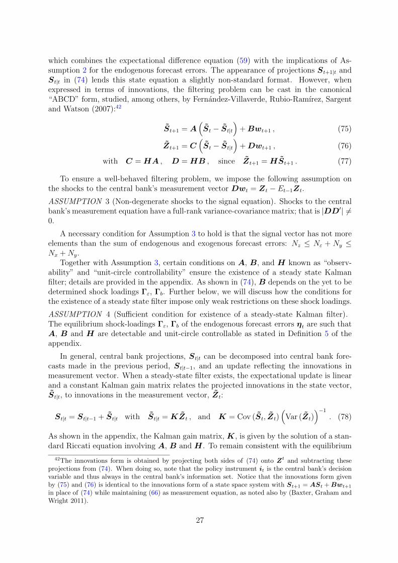
which combines the expectational difference equation (59) with the implications of As-sumption 2 for the endogenous forecast errors. The appearance of projections St+1|t andSt|t in (74) lends this state equation a slightly non-standard format. However, whenexpressed in terms of innovations, the filtering problem can be cast in the canonical“ABCD” form, studied, among others, by Fernandez-Villaverde, Rubio-Ramırez, Sargentand Watson (2007):42
St+1 = A(St − St|t
)+Bwt+1 , (75)
Zt+1 = C(St − St|t
)+Dwt+1 , (76)
with C = HA , D = HB , since Zt+1 = HSt+1 . (77)
To ensure a well-behaved filtering problem, we impose the following assumption onthe shocks to the central bank’s measurement vector Dwt = Zt − Et−1Zt.
ASSUMPTION 3 (Non-degenerate shocks to the signal equation). Shocks to the centralbank’s measurement equation have a full-rank variance-covariance matrix; that is |DD′| 6=0.
A necessary condition for Assumption 3 to hold is that the signal vector has not moreelements than the sum of endogenous and exogenous forecast errors: Nz ≤ Nε + Ny ≤Nx +Ny.
Together with Assumption 3, certain conditions on A, B, and H known as “observ-ability” and “unit-circle controllability” ensure the existence of a steady state Kalmanfilter; details are provided in the appendix. As shown in (74), B depends on the yet to bedetermined shock loadings Γε, Γb. Further below, we will discuss how the conditions forthe existence of a steady state filter impose only weak restrictions on these shock loadings.
ASSUMPTION 4 (Sufficient condition for existence of a steady-state Kalman filter).The equilibrium shock-loadings Γε, Γb of the endogenous forecast errors ηt are such thatA, B and H are detectable and unit-circle controllable as stated in Definition 5 of theappendix.
In general, central bank projections, St|t can be decomposed into central bank fore-casts made in the previous period, St|t−1, and an update reflecting the innovations inmeasurement vector. When a steady-state filter exists, the expectational update is linearand a constant Kalman gain matrix relates the projected innovations in the state vector,St|t, to innovations in the measurement vector, Zt:
St|t = St|t−1 + St|t with St|t = KZt , and K = Cov (St, Zt)(
Var (Zt))−1
. (78)
As shown in the appendix, the Kalman gain matrix, K, is given by the solution of a stan-dard Riccati equation involving A, B and H . To remain consistent with the equilibrium
42The innovations form is obtained by projecting both sides of (74) onto Zt and subtracting theseprojections from (74). When doing so, note that the policy instrument it is the central bank’s decisionvariable and thus always in the central bank’s information set. Notice that the innovations form givenby (75) and (76) is identical to the innovations form of a state space system with St+1 = ASt +Bwt+1
in place of (74) while maintaining (66) as measurement equation, as noted also by (Baxter, Graham andWright 2011).
27

properties laid out in Definition 1, we limit attention to the case when a steady-stateKalman filter exists, which enables us to represent the central bank’s conditional expec-tations as a recursive system of linear projections with time-invariant coefficients.
Proposition 3 (Existence of steady-state Kalman filter). When Assumptions 3 and 4hold, a steady state Kalman filter exists that describes the projection of innovations inthe state vector, St|t = KZt with a constant Kalman gain K as in (78). Moreover, thevariance-covariance matrix of projection residuals is constant, Var
(St|Zt
)= Var (S∗t ) =
Σ∗. Existence of a steady state Kalman filter ensures that innovations St = St − St|t−1and residuals S∗t = St − St|t are stationary. Innovations to the measurement equation,
Zt, are stationary as well.
Proof. See Theorem 3 of Appendix A. The stationarity of Zt = HSt follows then fromthe stationarity of St.
Equation (78) describes the update from policymaker forecasts, St|t−1, to currentprojections, St|t. What remains to be characterized is the transition equation from pol-icymakers’ projections St|t to their forecasts, St+1|t, which is restricted by the lineardifference equations (59) and the rule (60) for the policy instrument it. Since the policyinstrument may depend on its own lagged value via Φi 6= 0 in (60), we construct the tran-sition from St|t to St+1|t based on the vector St, which includes St and it−1, as definedin (67).
Conditioning down (59) and (60) onto the information set of the policymaker, Zt,yields a system of expectational linear difference equations in St that is akin to the full-information system shown in (68), except for the use of policymaker projections in lieu offull-information expectations:
JSt+1|t = ASt|t (79)
with J , and A as defined in (68) above. In a stationary equilibrium consistent withDefinition 1, St is stationary, and so is its projection St|t. When the equilibrium is linearand time-invariant, the projections St|t must follow
St+1|t = T St|t , with (JT −A)St|t = 0 for some stable matrix T . (80)
T spans a stable, invariant subspace of the matrix pencil |J z−A|. In principle, severalchoices of T could satisfy this criterion. To see this, think of any T whose columns includea (sub)set of stable eigenvectors of the pencil plus columns of zeros. The simple exampleof Section 2, is characterized by a dynamic system with only two non-zero eigenvalues,and a single, one-dimensional stable subspace of the associated matrix pencil. In thiscase, there is a single choice of T consistent with the equilibrium, and it is identical tothe full-information transition matrix T .
In addition, JT − A must be orthogonal to the space of projections St|t. Beforediscussing further the determination of T , note that in a linear equilibrium with normallydistributed shocks with a given linear transformation from projections St|t into forecastsSt+1|t, the Kalman filter represents conditional expectations of St (and thus also St).
Proposition 4 (Kalman filter represents conditional expectations). When the conditionsfor Proposition 3 hold, and for a given stable transition matrix T between policymaker
28

projections and forecasts as in (80), the steady state Kalman filter represents conditionalexpectations St|t = E
(St|Zt
)in a linear, time-invariant stationary equilibrium. For a
given sequence of innovations in the measurement vector, Zt, the Kalman filter impliesthe following, stationary evolution of projections:
St+1|t+1 = T St|t +KZt+1 , with K =
0Kx
Ky
Ki
(81)
Proof. In a linear, time-invariant stationary equilibrium shocks are jointly normal andpropagate linearly so that the sequences of St and Zt are joint normally distributed, sothat conditional expectations are identical to mean-squared-error optimal linear projec-tions. By the law of iterated projections, we can decompose
E(St+1|Zt+1
)= E
(St+1|Zt
)+ E
(St+1|Zt+1
)and we have E
(St+1|Zt
)= T St|t based on (80). E
(St+1|Zt+1
)= KZt+1 follows
from Proposition 3. Kx and Ky are appropriate partitions of K as defined in (78) and
Ki = Cov(it, Zt
)(Var
(Zt
))−1.43 The upper block of K, corresponding to the Kalman
gain coefficients for the lagged policy instrument, are zero since it−1 = it−1|t−1 and thus
it−1|t = it−1|t − it−1|t−1 = 0.
3.4 A Class of Imperfect Information Equilibria
As noted above, there can be multiple solutions for T in (80). As an application ofcertainty equivalence, a valid choice for T is T , known from the full-information solu-tion given in (70).44 In the full-information case, and under the maintained assumptionthat Assumption 1 holds, T characterizes the unique solution to the difference equationJEtSt+1 = ASt.
In the imperfect information case, T need not be a unique solution. However, themultiplicity of equilibria highlighted in our paper does not stem from the implications ofchoosing different T . We rather focus solely on equilibria based on T = T , which is con-sistent with the approach of Svensson and Woodford (2004) who assume that equilibriumis unique in a setup similar to ours.45. In order to ensure T = T , we follow Svensson andWoodford (2004) and impose the following condition:46
43The value for Ki could be computed based on the policy rule (60) and the dynamics of St; however,further below we utilize a more direct approach.
44To verify the validity of T as a solution to (79), note that T solves (68) and that (79) represents thesame difference equation, when projected onto Zt.
45Applications that build on Svensson and Woodford (2004) are, for example, Dotsey and Hornstein(2003), Aoki (2006),Nimark (2008b), Carboni and Ellison (2011).
46Note that (80) corresponds to their equation (42), and that our projection condition (82) correspondsto their (42), (45), (46), and (47).
29

Definition 2 (Projection Condition). The projection condition restricts the mappingbetween projected backward- and forward-looking variables to be identical to the full-information case:
Y t|t = GX t|t , and X t+1|t = PX t|t . (82)
where G and P are the unique solution coefficients in the corresponding full-informationcase.
The projection condition is an equilibrium condition that imposes a linear mappingbetween projections of backward- and forward-looking variables. In particular, the pro-jection condition imposes a second-moment restriction on the joint distribution of theinnovations X t, Y t.
47 As a second-moment restriction, the projection condition restrictsonly co-movements of the innovations on average but not for any particular realizationof X t and Y t. The upshot of the projection condition (82) is the following restrictionbetween Kalman gains of forward- and backward-looking variables:
Y t|t = Gyx X t|t + Gyi it−1|t =⇒ Y t|t = Gyx X t|t ⇐⇒ (Ky − Gyx Kx) Zt = 0 ,(83)
where Ky and Kx denote the corresponding partitions of the Kalman gain, K, defined
in (78).48 Since (83) must hold for every Zt, the projection condition implies a restrictionon the Kalman gains, summarized in the following proposition.
Proposition 5 (Projection Condition for Kalman gains). The projection condition (82)holds only if the Kalman gains satisfy Ky = Gyx Kx.
Proof. As noted in (83), a necessary condition for the projection to hold is (Ky − Gyx Kx) Zt =
0 for all realizations of Zt, which has a joint normal distribution. Assumption 3 impliesthat Var (Zt) = C Var (S∗t )C
′+DD′ is strictly positive definite, so that the distributionof Zt is non-degenerate. For (83) to hold, we must have Ky = Gyx Kx.
Kalman gains are multivariate regression slopes.49 As a result of Proposition 5, theprojection condition imposes a linear restriction on covariances between Y t, X t, and Zt,i.e. Cov (Y t, Zt) = Gyx Cov (X t, Zt).
Henceforth we only consider equilibria that are stationary, linear and time-invariantaccording to Definition 1 and that satisfy the projection condition laid out in Definition 2.In such equilibria, the dynamics of forward- and backward-looking variables, as well asthe policy instrument, are characterized by a state vector that tracks both projections andactual values of the vector St, which contains backward- and forward-looking variablesas well as the policy instrument. In fact, the joint vector of St and St|t does not needto tracked in its entirety: First, St includes the policy instrument it, which lies in the
47In addition to Y t and Xt, Yt and X t also contain the current and lagged policy instrument, re-spectively. However, the projection condition does not impose a direct restriction on innovations in thepolicy instrument since it = it|t and thus it−1|t = it−1|t − it−1|t−1 = 0.
48That means K =[K ′x K ′y
]′so that Kx = Cov (Xt, Zt)
(Var (Zt)
−1), and Ky =
Cov (Y t, Zt)(
Var (Zt)−1)
.
49Please recall that Ky = Cov (Y t, Zt) Var (Zt)−1
and Kx = Cov (Xt, Zt) Var (Zt)−1
.
30
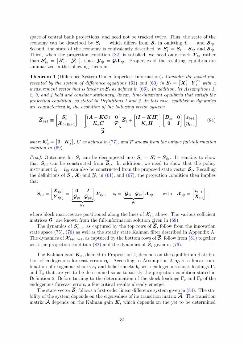
space of central bank projections, and need not be tracked twice. Thus, the state of theeconomy can be described by St — which differs from St in omitting it — and St|t.Second, the state of the economy is equivalently described by S∗t = St − St|t and St|t.Third, when the projection condition (82) is satisfied, we need only track X t|t ratherthan S ′t|t =
[X ′t|t Y ′t|t
], since Y t|t = GX t|t. Properties of the resulting equilibria are
summarized in the following theorem.
Theorem 1 (Difference System Under Imperfect Information). Consider the model rep-
resented by the system of difference equations (61) and (60) in St =[X ′t Y ′t
]′with a
measurement vector that is linear in St as defined in (66). In addition, let Assumptions 1,2, 3, and 4 hold and consider stationary, linear, time-invariant equilibria that satisfy theprojection condition, as stated in Definitions 1 and 2. In this case, equilibrium dynamicsare characterized by the evolution of the following vector system:
St+1 ≡[S∗t+1
X t+1|t+1
]=
[(A−KC) 0KxC P
]︸ ︷︷ ︸
A
St +
[(I −KH)KxH
] [Bxε 00 I
] [εt+1
ηt+1
](84)
whereK′x =[0 K ′x
], C as defined in (77), and P known from the unique full-information
solution in (69).
Proof. Outcomes for St can be decomposed into St = S∗t + St|t. It remains to showthat St|t can be constructed from St. In addition, we need to show that the policyinstrument it = it|t can also be constructed from the proposed state vector St. Recallingthe definitions of St, X t and Y t in (61), and (67), the projection condition then impliesthat
St|t =
[X t|tY t|t
]=
[0 IGyi Gyx
]︸ ︷︷ ︸
GS
X t|t , it =[Gii Gix
]︸ ︷︷ ︸Gi
X t|t , with X t|t =
[it−1X t|t
],
where block matrices are partitioned along the lines of X t|t above. The various cofficientmatrices G·· are known from the full-information solution given in (69).
The dynamics of S∗t+1, as captured by the top rows of S, follow from the innovationstate space (75), (76) as well as the steady state Kalman filter described in Appendix A.The dynamics of X t+1|t+1, as captured by the bottom rows of S, follow from (81) together
with the projection condition (82) and the dynamics of Zt given in (76).
The Kalman gain Kx, defined in Proposition 4, depends on the equilibrium distribu-tion of endogenous forecast errors ηt. According to Assumption 2, ηt is a linear com-bination of exogenous shocks εt and belief shocks bt with endogenous shock loadings Γε
and Γb that are yet to be determined so as to satisfy the projection condition stated inDefinition 2. Before turning to the determination of the shock loadings Γε and Γb of theendogenous forecast errors, a few critical results already emerge.
The state vector St follows a first-order linear difference system given in (84). The sta-bility of the system depends on the eigenvalues of its transition matrix A. The transitionmatrix A depends on the Kalman gain K, which depends on the yet to be determined
31

shock loadings Γε and Γb of the endogenous forecast errors ηt. Nevertheless, as arguednext, the existence of a steady-state Kalman filter allows us to conclude that A, is stable.
Corollary 1 (Stable Transition Matrix). Provided that a steady-state Kalman filter exists,the transition matrixA in (84) is stable. The eigenvalues ofA are given by the eigenvaluesof P, which is stable and known from the full-information solution (69), and A −KC,whose stability is assured by the existence of the steady-state Kalman filter.
Proof. The stability of P follows from Assumption 1 and the resulting solution of thefull-information case in (114). The stability of A − KC follows from Theorem 3 inAppendix A.
The upshot of Corollary 1 is that the usual root-counting arguments do not pin downthe shock loadings Γε and Γb of the endogenous forecast errors ηt+1 in (84), since A is astable matrix for any choice of Γε and Γb consistent with the existence of a steady stateKalman filter. Moreover, the projection condition does typically not place sufficientlymany restrictions on Γηε and Γηb to uniquely identify the shock loadings:
Corollary 2 (Generic Indeterminacy). With A stable, the endogenous forecast errors areonly restricted by the projection condition given in Definition 2. The shocks loadings ofthe endogenous forecast errors, Γε and Γb, have Ny × (Nε + Ny) unknown conditions.Stated as in (83), the projection condition imposes only Ny×Nz restrictions. However, anecessary condition for Assumption 3 to hold is Nz ≤ Nε+Ny. As a result, the projectioncondition cannot uniquely identify the shock loadings Γε and Γb.
Among others, Theorem 1 rests on the assumption of joint detectability and unit-circlecontrollability of (A,B,H) where B depends on the endogenous shock loadings Γε andΓb while A and H are primitives of the model setup. The detectability condition canthus be verified independently from solving for Γε and Γb. An addition, as described inthe appendix (see Proposition 8), a full rank of
B =
[Bxε 0Γε Γb
]is sufficient to ensure unit-circle controllability . As part of the model setup, Bxε issupposed to have full rank. Consequently, the criterion of a full rank of B is satisfiedwhen the belief shock loadings Γb have full rank, and thus Γb 6= 0. Non-zero belief shockloadings are a hallmark of equilibrium indeterminacy. While the projection conditionplaces restrictions on Γb, non-zero belief shock loadings are thus a sufficient condition forthe existence of a steady state Kalman filter, which in turn assures the stability of A.
Before turning to approaches to compute Γε and Γb that are consistent with theprojection condition, we summarize the construction of an equilibrium for a given solutionof the endogenous forecast errors.
Theorem 2 (Equilibria under Imperfect Information). Consider the difference systemunder characterized in Theorem 1 and let ηt = Γεεt + Γbbt with shock loadings Γε andΓb such that the projection condition (82) is satisfied. Equilibrium outcomes are then
32

characterized as follows:
St =[I Gs
]St it =
[0 Gi
]St St+1 = A St + B wt+1 , (85)
with St ≡[S∗tX t
], wt+1 ≡
[εt+1
bt+1
], and B ≡
[(B −KD)KXD
]. (86)
where B and D encode the shock loading Γε and Γb as stated in (77); Kx, Gs and Gi aredefined in the proof of Theorem 1. Block matrices are partitioned along the lines of St asstated above.
Proof. The proof follows straightforwardly from Theorem 1.
3.5 Determination of the Endogenous Forecast Errors
As described by Sims (2002) and Lubik and Schorfheide (2003), restrictions for the en-dogenous forecast errors ηt emanate from explosive roots in the dynamic system. In ourimperfect information case, further restrictions result from the projection condition statedin Definition 2. As noted in Corollary 1 above, the transition matrix A is always stablein a time-invariant equilibrium with a steady-state Kalman filter. Restrictions on ηt canonly result from the projection condition; but as discussed in Corollary 2, the projec-tion condition does generally not provide sufficiently many restrictions to pin down ηtuniquely.
The determination of shock loadings Γε, Γb for the endogenous forecast errors thatare consistent with the projection condition poses an intricate fixed problem betweenshock loadings and Kalman gains. As noted already by Sargent (1991), the Kalmangains are endogenous equilibrium objects when the observable signals reflect informationcontained in endogenous variables. In contrast, the Kalman filtering problem can besolved independently of the equilibrium dynamics of the system, when the signal vectorconsists only of exogenous variables.
In (66), the central bank’s measurement vector is generically described as a linearcombination of backward- and forward-looking variables, Zt = HxX t + HyY t. Tofacilitate the analysis, we now delineate two cases: one where the signal depends onendogenous variables (specifically, choosing Hy = I) as well as the case where the signalsolely reflects exogenous variables (Hy = 0 and X t exogenous).
3.5.1 Endogenous Signal
In (66), the signal observed by the central bank involves a linear combination of forward-and backward-looking variables, such that the signal depends at least in part on endoge-nous variables. When considering this case, and to simplify some of the algebra, we limitourselves to signal vectors that have the same length as the vector of forward-lookingvariables (Y t) and that have no rank-deficient loading on Y t. All told, we assume thatHy in (66) is square and invertible. In this case, Hy can be normalized to the identity
33

matrix.50 In the endogenous-signal case, we thus consider signal vectors of the form
Zt = HxX t + Y t and thus H =[Hx I
]. (87)
Note that the endogenous-signal setup also includes the case where each forward-looking variable is observed with error, as in Zt = Y t + νt where νt is an exogenousmeasurement error to be included among the set of backward-looking variables in X t.
In the context of the simple example described in section 2, we provided an analyticalcharacterization of the fixed point problem posed by the endogenous-signal case. However,even in this stylized example the fixed point proved intractable to solve analytically.Instead, we have derived a fast numerical procedure to solve for shock loadings Γε, Γb
that are consistent with the projection condition for this case.Our numerical approach combines elements of standard techniques for solving lin-
ear RE models with a fast algorithm to solve the non-linear fixed-point problem for theRiccati equation embedded in the Kalman filter while ensuring consistency with the pro-jection condition. For a given intial guess of Γε, Γb, the procedure returns values that areconsistent with the projection condition; different starting values then generate typicallydifferent result values. Details of our algorithm are described in Appendix B.
3.5.2 Exogenous Signal
For the case of an exogenous signal, we derive two general results: First, the projectioncondition does not restrict the belief shock loadings of the endogenous forecast errors,Γb, when the signal is exogenous. Second, we derive an analytical expression for therestrictions on the loadings of the endogenous forecast errors on fundamental shocks(including the measurement errors) that result from the projection condition.
To consider the case of a purely exogenous signal, we need to distinguish betweenendogenous and exogenous components of the vector of backward-looking variables X t.Let X t be partitioned into exogenous variables, denoted X1
t , and endogenous variables(like the lagged inflation rate in case of a Phillips Curve with indexation), denoted X2
t .Exogeneity of X1
t places zero restrictions on the system matrices in (59), and itsdynamics reduce to
X1t = A11
xxX1t−1 +B1
xε εt (88)
where A11xx and B1
xε are appropriate sub-blocks of A and Bxε.51. The signal is then given
byZt = HxX
1t . (89)
50Consider the case of a signal Zt = HxXt + HyY t where Hy is square and nonsingular. The
information content provided by Zt is equivalent to what is spanned by Zt = H−1y Zt with Hx =
H−1y Hx.51Consistent with (59) , the endogenous component of Xt generally evolves according to
X2t = A21
xxX1t−1 +A22
xxX2t−1 +A2
yx Y t−1 + A21
xxX1t−1|t−1 + A
22
xxX2t−1t−1 + A
2
yx Y t−1|t−1 +B2xε εt ,
whereA21xx,A22
xx,A2yx, A
21
xx, A22
xx, A2
yx, andB2xε are appropriate sub-blocks ofA, A andBxε, respectively.
34

For ease of notation, we consider henceforth the case where the entire vector ofbackward-looking variables is exogenous; that means X t = X1
t . (Our first result inthis section, the lack of restrictions on Γb, extends also to the case when X t containsan endogenous component, that is, however, not reflected by the signal.) The signalextraction problem is then given by the following system:
X t = AxxX t−1 +Bxεεt , (90)
Zt = HxX t , (91)
where Axx denotes the appropriate sub-block of A in (59).Existence of steady state Kalman filter is assured by joint detectability and unit-circle
controllability of (Axx,Bxε,H), which does not depend on the equilibrium solution of thesystem and thus a weaker condition than what is required by Assumption 4. Henceforth,existence of a steady-state Kalman filter is assumed, resulting in a constant gain matrixKx such that Axx(I −KxHx) is stable.
A defining feature of the exogenous-signal case is that the signal extraction problemcan be solved independently from the dynamics of the forward-looking variables, Y t andKx and Var (X∗t ) are determined solely by (90) and (91). We have X∗t = X t −KxZt =(I −KxHx)X t and can thus write
X t = AxxX∗t−1 +Bxε = Axx(I −KxHx)X t−1 +Bxεεt (92)
Moreover, when X t = X1t , application of the projection condition translates the Kx
into a given Kalman gain for the forward-looking variables: Ky = GyxKx, where Gyx isknown from the full-information solution of the model. The innovation dynamics of theforward-looking variables are then restricted by the following transition equation:
Y t+1 = AyxX t−1 +AyyY t−1 + ηt+1 with Ayx = Ayx − (Ayx +AyyGyx)KxHx (93)
where the endogenous forecast errors, ηt, remain to be derived. As before, we seekηt = Γηε εt + Γηb bt, with loadings Γηε and Γηb that satisfy the projection condition.
In addition, in order to ensure stationarity of Y t, Ayy has to be a stable matrix orfurther restrictions need to be imposed on ηt. In our discussion of the general case,as part of Assumption 4, we imposed the requirement that (A,H) are detectable. Asdiscussed in Appendix A, this requirement is tantamount to letting the signal vector loadon any linear combinations of backward- and forward-looking variables associated withpotentially unstable dynamics. In the present context of a signal that does not load onY t, detectability of (A,H) boils down to the requirement that Ayy is a stable matrix.
If only the weaker requirement of detectability of (Axx,Hx) is to be imposed, note thatthe innovation system (92) and (93) has the form of a typical linear rational expectationssystem as analyzed, among others, by Klein (2000) and Sims (2002). As shown there,when Ayy is not a stable matrix, linear combinations of ηt associated with unstable
dynamics of Y t need to be set to zero. However, as illustrated in the simple example ofSection 2, this is typically not sufficient to uniquely determine equilibrium outcomes.52
52Note that (93) describes the innovation dynamics of the forward-looking variables, which do notdirectly depend on the policy rule coefficients Φ· in (60). Since the policy instrument always lies in thespace of observations of the policymaker, it drops out of the innovations dynamics of the forward-looking
35

The projection condition requires Cov (Y t, Zt) = Gyx Cov (X t, Zt). Due to the exo-
geneity of Zt — and thus Cov (bt, Zt) = 0 — this covariance restriction does not affectadmissible belief shock loadings Γηb.
53
Proposition 6 (Unrestricted Belief-Shock Loadings When the Signal is Exogenous).When the signal is exogenous, as given by (90) and (91), there are no restrictions on Γηb
in a stable, linear, time-invariant equilibrium (Definition 1) where the projection condition(Definition 2) holds.
Proof. Formally, we can decompose Y t into two pieces: a component, Yε
t , that reflects
the history of fundamental shocks εt and another component, Yb
t , solely driven by beliefshocks.
Y t+1 = Yε
t+1 + Yb
t+1 (94)
Yε
t+1 ≡ AyxX t−1 +AyyYε
t−1 + Γηεεt+1 (95)
Yb
t+1 ≡ AyyYb
t−1 + Γηbbt+1 (96)
with the evolution of X t given by (92) and Ayx as defined in (93). When the measurementvector is exogenous, it is uncorrelated with belief shocks at all leads and lags. Accordingly,the central bank’s information set does not contain any signal about bt+h, for any h,
E(bt+h|Zt) = 0. Likewise, Yb
t is orthogonal to Zt, E(Y bt|Zt) = 0 for any Γηb. As a
consequence, Γηb does not affect the projection condition (83), Y t|t = Gyx X t|t.
As can be seen from the proof of Proposition 6, the underlying argument rests onthe orthogonality between the exogenous signal vector X t and the belief shocks bt. Theargument easily extends to the more general case when the vector of backward-lookingvariables X t contains both exogenous and endogenous components X1
t and X2t as de-
scribed in the previous section.Finally, for the case when X t = X1
t , we can derive simple expressions to constructfundamental shock loadings Γηε that satisfy the projection condition. Let W t ≡ Y
ε
t −GyxX t and note that the projection condition requires W t|t = 0 and thus W t = W
∗t .
54
Equivalently, the projection condition requires Cov (W t, Zt) = ΣwxH′ = 0 with Σwx ≡
Cov (W t, X t). Based on (90) and (95), and with Awx = Ayx − GyxAxx + AyyGyx, the
dynamics of W t are given by
W t+1 = AwxX∗t−1 +AyyW t−1 + (Γηε − GyxBxε)εt+1 (97)
Σwx = AwxΣ∗xxA
′xx +AyyΣwxA
′xx (I −KxHx)
′ + (Γηε − GyxBxε)B′xε (98)
where Σ∗xx = Var (X∗t ) is known from solving the steady-state Kalman filter. The onlyunknowns in (98) are Σwx and Γηε and we seek to find Γηε such that ΣwxH
′x = 0.
dynamics. However, in monetary policy models with interest rate rules, it is the appropriate choice ofpolicy coefficients that creates many possibly unstable dynamics (which cannot be part of a stationaryequilibrium) and just a single stationary outcome.
53Notice that the result also goes through, when part of the vector of backward-looking variables wasendogenous, as long as the signal remains exogenous.
54In light of Proposition 6, we can neglect the effects of belief shocks and W t has been defined withreference to Y
ε
t , as defined in the proof to Proposition 6.
36
Valid values of Σwx must lie in the nullspace ofH ′x. Specifically, given a (Nx−Nz)×Nx
matrix N such that NH ′ = 0.55 we can construct valid candidates for Σwx by choosingan arbitrary Ny × (Nx −Nz) matrix G and let Σwx = GN .
For a given candidate Σwx = GN , Γηε must thus satsfy the following condition:
ΓηεB′xε = f(G) (99)
where f(G) ≡ GN + GyxBxεB′xε −AwxΣ
∗xxA
′xx −AyyGNA
′xx (I −KxHx)
′ (100)
The ability to solve (99) for Γηε depends on the dimension of the problem. WhenNx = Nε, the number of exogenous variables is identical to the number of exogenousshocks, and Bxε is invertible. When |Bxε| 6= 0 it is straightforward to solve (99) for Γηε
given an arbitrary G:
Γηε = f(G)(B′xε)−1 . (101)
In case of Nx > Nε, there is not necessarily a Γηε that solves (99) for anyG. Instead,Gneeds to be chosen such that f(G) (I −Bxε(B
′xεBxε)
−1B′xε) = 0, which can be obtainednumerically.56 For such a choice of G, a valid Γηε is given by Γηε = f(G)Bxε(B
′xεBxε)
−1.
4 Quantitative Analysis
We now solve and analyze our modelling framework quantitatively. We first present resultsfor the simple example economy of Section 2 before turning to a New Keynesian economythat is widely used for the analysis of monetary policy. Both applications consider centralbank information sets that are spanned by endogenous signals as discussed in section 3.5.When the central bank’s measurement vector reflects endogenous variables, analyticalsolutions are difficult to obtain and we therefore rely on our numerical procedure.
4.1 Quantitative Results for the Simple Example Model
An analytical characterization of equilibria in the simple example economy under exoge-nous and endogenous information sets are provided in Propositions 1 and 2 in section 2.Nevertheless, analytical bounds on parameters for existence of a solution remain difficultto derive, especially in the case of an endogenous information set. In this section, weprovide further insight into the mechanics and implications of our framework by solvingthe model numerically. Our numerical solution algorithm combines elements of standardtechniques for solving linear RE models with a fast algorithm to solve the non-linear fixed-point problem for the Riccati equation embedded in the Kalman filter and the projectioncondition. Specifically, the numerical algorithm searches for shock loadings γε, γν , and γbthat satisfy the projection condition in the endogenous signal case. Further details canbe found in Appendix B.
55A matrixN such thatNH ′ = 0 can readily be obtained from the SVD decomposition ofH = USV ′
where U and V are orthonormal, S =[S1 0
]and S1 is a Nz × Nz diagonal matrix. Partition V
conformably into V =[V 1 V 2
]such that H = US1V
′1. Since V is orthonormal we have V ′2V 1 = 0.
Choosing N = V ′2 then ensures NH ′ = 0.56Note that, as introduced in (62), Bxε has full rank which ensures that |B′xεBxε| 6= 0.
37

We consider the baseline case of the policy rule it = φπt|t where the endogenousinformation set Zt = πt + νt. For purposes of illustration, we set the policy parameterφ = 1.5 and assume that the real rate follows an AR(1) process with persistence ρ = 0.9and a unit innovation variance σ2
ε = 1. Initial experimentation shows that in this simpleexample the measurement error on inflation has to be large for an equilibrium to exist. Wetherefore set the variance of the i.i.d. measurement error νt to σ2
ν = 2.52.57 We generate2000 starting points from which our algorithm is able to find valid equilibria in 99 percentof all cases. Each equilibrium is associated with a triple (γε, γb, γν) of loadings on theshocks in the forecast error decomposition. The fact that there are multiple such loadingsfor the parameter space simply reflects that the RE solution is indeterminate. In sectionI.1 of the Supplementary Appendix, we explore the bounds of the existence region for thisparameterization numerically.
We plot impulse responses to each shock for the entire set of equilibria in Figure 1,while impulse responses for a specific equilibrium as an example are displayed in Figure 2.For reference, we also plot the impulse responses for the FIRE specification. In the lattercase, a unit innovation to the real rate raises inflation by 1/ (φ− ρ) = 5/3 which thendecays at the constant rate ρ. The interest response follows the same pattern. Thissimply reflects the Fisher effect in that a higher real rate requires a higher nominal rateand in turn a higher inflation rate. The unique FIRE equilibrium has zero response tothe measurement error since the model is not defined as having such error, but also tothe belief shock since the solution is unique under the given parameterization.
Under LIRE, however, the set of equilibria is notably different. On impact, a unitinnovation in the real rate can either lead to an increase or a decrease in inflation over arange of about (−1.9, 1.7) depending on which indeterminate equilibrium the economy isin. Similarly, the nominal rate response can be positive or negative. In effect, in differentLIRE equilibria, inflation and the nominal rate can comove positively or negatively. Fig-ure 2 displays impulse response for one of the possible LIRE equilibria where, in contrastto the FIRE solution, inflation and the nominal interest rate comove negatively. Whilethe nominal rate follows the real rate increase, inflation can fall on account of a negativeloading γε on the forecast error (see Proposition 2). The figure also shows that a unitmeasurement error shock lowers inflation and the nominal rate which indicates a nega-tive loading on νt in the solution, γν < 0 (see Proposition 2). Therefore, no equilibriumexists for positive γν .
58 In contrast, the responses to the belief shock are symmetric andunrestricted, similar to the case of an exogenous information set.59
Figure 3 reports the autocorrelation function (ACF) and the standard deviation rel-ative to the full information scenario.60 As shown in the upper row of panels, the FIREsolution displays the typical autocorrelation pattern of a first-order autoregressive pro-
57As discussed in section 2, the variance of the belief shock σ2b is normalized to unity without loss of
generality.58This is confirmed by Figure 2 in the Supplementary Appendix59The findings are reminiscent of the observation by Lubik and Schorfheide (2004) that changes in
comovement patterns are a hallmark of equilibrium indeterminacy and thereby allow econometricians toidentify different sets of equilibria. Moreover, their observation that indeterminate equilibria do imposesome restrictions on the behavior of the economy in response to fundamental shocks thus carries over toour framework.
60Moments are computed via simulation for 20,000 periods with the first 1,000 periods discarded asburn-in to avoid dependence on initial conditions.
38

Figure 1: IRFs of Various Equilibria in Fisher economy
Note: Impulse response functions (IRF) for the Fisher economy model under full informa-tion (blue) as well as various limited-information equilibria (red). Each row represents theresponse of a specific variable to the shocks in the model whereas each column representthe responses of the endogenous variables to a specific shock.
39

Figure 2: Example IRF from an Equilibrium in the Fisher economy
0 4 8 12 16-2
-1
0
1
2
0 4 8 12 16-5
-4
-3
-2
-1
0
0 4 8 12 16-0.3
-0.2
-0.1
0
0.1
0.2
0 4 8 12 160
0.5
1
1.5
2
2.5
i
0 4 8 12 16
-1.5
-1
-0.5
0
0 4 8 12 160
0.05
0.1
0.15
0.2
Note: Impulse response functions (IRF) for the Fisher economy model under full infor-mation (blue) as well as an example from the limited-information equilibria (red).
40

Figure 3: Second moments of limited-information equilibria in Fisher economy
Note: Top panels show moments of endogenous variables for the Fisher economy model un-der full information (blue) as well as various limited information equilibria (red). Bottompanel reports ranges of relative standard deviations of outcomes under limited informationrelative to the full-information outcomes.
41

cess. Comparing the set of outcomes under LIRE against the unique FIRE equilibrium,the persistence of inflation is generally lower and its serial correlation decays much morerapidly under LIRE, whereas for the nominal rate the ACF closely resembles that underFIRE. Since it = φπt|t = φ
φ−ρrt|t the nominal rate behaves like the real rate projection.Given the solution in Proposition 2, this implies that the Kalman gain κr is in a tightneighbourhood around zero. The lower panel of the figure shows ranges of relative stan-dard deviations of outcomes under LIRE relative to the respective FIRE outcomes. Theinterest rate under LIRE is generally less volatile than its FIRE counterpart despite thepresence of two additional shocks. The lower interest-rate volatility echoes our discussionin section 2 that the effective response to inflation under LIRE after taking into accountthe filtering problem constitutes a violation of the Taylor principle. In the LIRE case,imperfect information prevents the central bank from moving the policy rate aggressivelyin response to actual inflation. Instead, optimal filtering leads to attenuation of the policyresponse, the flipside of which is heightened inflation volatility.
4.2 Quantitative Results for a New Keynesian Model
We now specify and solve a standard New Keynesian model often used in monetary policyanalysis under the assumption that the monetary authority has a limited informationset. Akin to the simple example model, we assume that there is a private sector, ahousehold, that has the same information set as households in the full information versionof the model. We also assume that the central bank only observes noisy measurements ofinflation and the level of real GDP. Finally, the central bank follows a monetary policyrule in which it reacts to its best estimate of inflation and the output gap.
We consider a version of the New Keynesian model that includes a Phillips curve witha backward-looking component in inflation πt:
(1− γβ)πt = βEtπt+1 + γπt−1 + xt, (102)
where 0 ≤ γ < 1 denotes the degree of indexation and governs inflation persistence. xt isthe output gap and the sole driver of inflation in this model. Its evolution is captured bya variant of the Euler-equation which relates output to the real rate and policy actions:
xt = Etxt+1 −1
σ(it − Etπt+1 − rt) . (103)
σ > 0 is the intertemporal substitution elasticity and governs the responsiveness of outputgrowth to interest rate movements. The term in parentheses is the gap between the actualreal rate of interest (it − Etπt+1) and its natural rate rt. Similar to Laubach and Williams(2003), we assume that rt is related to expected growth in potential real GDP yt:
rt = σEt∆yt+1. (104)
Furthermore, we assume that ∆yt follows an autoregressive process of order one:
∆yt = ρy∆yt−1 + εyt , (105)
where the innovation εyt is i.i.d. Gaussian with zero mean and finite variance σ2y, namely
42

εyt ∼ N(0, σ2
y
).
The central bank follows the feedback rule:
it = φππt|t + φxxt|t, (106)
where we assume that the policy coefficients φπ and φx are such that in the FIRE coun-terpart of this model the equilibrium is unique. As before, xt|t denotes the output gapprojection given information available to the central bank at time t. The signal extractionproblem is thus somewhat more involved than in the simple example. The central banknot only has to infer the true level of output from its noisy signal, but it also has to inferthe best estimate of the output gap from the available data. We choose this specificationas it arguably mirrors more closely the practice of many central banks, including theFederal Reserve.
We introduce two measurement errors in inflation and the level of output, νπt and νxt ,respectively. The measurement errors are jointly normally distributed and serially andmutually uncorrelated with variances σ2
π and σ2x. The level of GDP is by construction
equal to the growth rate in potential GDP plus the sum of lagged potential GDP and thecurrent output gap. This specification implies the following measurement vector Zt:
61
Zt =
[πt + νπt
∆yt + yt−1 + νxt + xt
], with
[νπtνxt
]∼ N
(0,
[σ2π 0
0 σ2x
]). (107)
Table 1: Parameters for NK model
Symbol Description Value
β Discount Factor 0.99σ Substitution Elasticity 1.00φ Labor Elasticity 1.00γ Inflation Indexation 0.25φπ Policy Coefficient 2.50φx Policy Coefficient 0.50ρy AR(1) - Coefficient 0.75σy StD. Output Growth 0.30σπ StD. Measurement Error 0.80σx StD. Measurement Error 1.39κ Composite Parameter 0.17
Note: Parameter values for the numerical analysis of the NK model.
We calibrate the model by choosing standard parameter values in the literature (see
61As written, the measurement vector Zt contains the level of output and thus a unit root. However,this unit root affects only the measurement dynamics and not the linear difference system of the NewKeynesian model, given by (102), (103) and (106). The conditions for the existence of a steady stateKalman Filter, described in Appendix A, remain satisfied. Since central bank projections are conditionedon the infinite horizon history of Zt, the measurement vector could equivalently be written in terms ofoutput growth.
43

Table 1). We set the intertemporal substitution elasticity to σ = 1 to maintain compa-rability with the simple example, while β = 0.99. The indexation parameter is chosen asγ = 0.25 which roughly replicates observed inflation persistence. The policy coefficientsφπ and φx are set to 2.5 and 0.5 which guarantees the existence of equilibria in a wideneighborhood of the parameterization. We calibrate the measurement error processes inline with the empirical findings in Lubik and Matthes (2016). For inflation, we choosethe standard deviation of our measurement error to match their estimated unconditionalstandard deviation for the inflation error.62 For real GDP, we assume that log GDP ismeasured with iid error. This automatically induces autocorrelation in the measurementerror for the log-difference of GDP, consistent with their findings.63
Figure 4 reports impulse response functions under FIRE and LIRE for the fundamentalshock to potential GDP growth in the left column, next to the two measurement errorsand the two belief shocks, denoted ηπ and ηx. Each row shows the response of the model’sendogenous variables. Solid blue lines indicate the responses under FIRE while the lines,or areas, in red capture the responses for different equilibria under LIRE. The differentresponses under LIRE are driven by different shock loadings γ, which are not uniquelydetermined in equilibrium. As the only shock under FIRE that affects outcomes theinnovation to potential GDP growth increases the natural real rate via the expectationschannel. This prompts a rise in the policy rate and reduces expected output gap growthon impact due to a fall in the current output gap. As actual production ramps up to closethe gap, inflation declines from its initial peak, which is driven by the relative reductionin supply on impact.
Under LIRE the impulse responses to the fundamental innovation are qualitativelysimilar to the FIRE responses although they show a somewhat richer dynamic adjustmentpattern. Figure 5 shows impulse responses for a single LIRE equilibrium that are fairlyclose to their FIRE counterparts. We also note that the FIRE response is in parts anenvelope to the area of responses associated with indeterminate LIRE equilibria, a patternwe also observe in the simple model. In the Supplementary Appendix, we report resultsfrom a specification where the measurement errors are small so that the signal contentof incoming data is high. While this specification still implies indeterminate equilibriaunder LIRE, the impulse responses to the fundamental shock essentially coincide withthe FIRE ones. Moreover, the responses to the other shocks are an order of magnitudesmaller and would likely be hard to detect in data. This distinguishes our frameworkfrom more standard indeterminacy results where the range of equilibria is considerablywider.64
The next two columns in Figure 4 show the responses to the measurement error shocks.A positive shock to νπt prompts the central bank to adjust its inflation projection upwards.
62In their paper, the measurement error in inflation is estimated to be mildly autocorrelated, witha point estimate of around 0.1 for the autoregressive coefficient. The switch from an autoregressivemeasurement error process to iid seems innocuous.
63In that case the standard deviation of the measurement error in the log-difference is twice the standarddeviation of the measurement error in levels. We match the standard deviation of the iid measurementerror to half of the unconditional standard deviation of the estimated measurement error for GDP growth.Standard deviations of all shocks are expressed in annualized percentages.
64In addition, in the New Keynesian model the impulse responses do not extend over the zero lineand thereby do not offer varying comovement patterns under indeterminacy as is the case in the simpleexample or in Lubik and Schorfheide (2004).
44

Figure 4: IRFs of Various Equilibria in New Keynesian model
Note: Impulse response functions (IRF) for the New Keynesian model under full informa-tion (blue) as well as various limited-information equilibria (red). Each row represents theresponse of a specific variable to the shocks in the model whereas each column representthe responses of the endogenous variables to a specific shock. An example of the IRF ofone of the limited-information equilibria is show in Figure (5).
45

Figure 5: IRF in New Keynesian model: Example of a limited information equilibrium
0 4 8 12 16
0
0.1
0.2
0.3
0.4 y
0 4 8 12 16
-0.4
-0.3
-0.2
-0.1
0
0 4 8 12 16
-0.01
0
0.01
0.02
x
0 4 8 12 16
0
0.01
0.02
0.03
0.04
0 4 8 12 16
-0.01
0
0.01
0.02
x
0 4 8 12 16
-0.6
-0.4
-0.2
0
x
0 4 8 12 16
-0.2
0
0.2
0.4
0 4 8 12 16
-0.06
-0.04
-0.02
0
0 4 8 12 16
-0.1
-0.05
0
0 4 8 12 16
-0.04
-0.02
0
0.02
0.04
0 4 8 12 16
0
0.1
0.2
0.3
0.4
i
0 4 8 12 16
-0.2
-0.1
0
0.1
0.2
0 4 8 12 16
-0.02
0
0.02
0.04
0 4 8 12 16
0
0.01
0.02
0.03
0.04
0 4 8 12 16
-0.02
0
0.02
0.04
Note: Impulse responses for one example (red) of the limited-information equilibria of theNew Keynesian model shown in Figure 4. (Full-information IRF in blue.)
46

This stimulates a contemporaneous rise in the policy rate and generally lowers the outputgap due to a fall in current GDP. The inflation rate falls because of the contractionarycentral bank policy response to the inflation mismeasurement. This pattern is also evi-dent from Figure 5. However, there are equilibria where this pattern is overturned witha considerably smaller, even negative, interest rate response. What drives these differ-ences are the different values of the endogenous Kalman gain associated with variousindeterminate equilibria. That is, equilibria exist where the responsiveness of inflationprojections to measurement error is small enough so that the standard adjustment dy-namics in response to output gap movements and their projections dominate. Responsesto the output measurement error follow a similar but less pronounced pattern. A positiveinnovation νxt leads to an upward revision of output gap projections and an interest ratehike, followed by a decline in current output and a rise in prices. Adjustment patterns toboth measurement errors exhibit slowly adjusting and oscillating dynamics.
Finally, the last two columns in Figure 4 show the responses to the belief shocks, whichare identical and symmetric.65 The graphs confirm the results of Lubik and Schorfheide(2003) and Farmer, Khramov, and Nicolo (2015) that sunspot shocks have a representa-tion that map into belief shocks; that is, they affect expectations directly, but to whichexpectational variable the belief shocks are appended do not affect outcomes for any givenequilibrium. Moreover, the set of impulse response functions is symmetric around the zeroline since the response to a sunspot shock in each equilibrium is only determined up toits sign. Nevertheless, we can still trace out the effect of, for instance, a positive beliefshock to inflation such as in the fourth column of Figure 5, where we plot the responsesfor one specific equilibrium.
To understand the equilibrium depicted in Figure 5, suppose consumers believe in-flation to be higher than initially anticipated, the belief being driven by the realizationof a sunspot that is interpreted as fundamental. This leads the central bank to raise itsinflation projection somewhat, but not fully given its filtering problem. The policy raterises, but not to the full extent required to invalidate consumers’ beliefs. This would occurif the policy response were such that it raised the real rate by enough to reign in increasedspending and thus rising prices. Although the central bank obeys the Taylor principle,the wedge between private sector and central bank expectations generated by the filter-ing process is sufficient for indeterminacy to arise. The less than aggressive interest-rateresponse thereby leads to output gap movements that validate beliefs to the extent thatinflation rises by enough.
We compute autocorrelation functions and relative standard deviations for the NewKeynesian model which are reported in Figure 6. The upper panel shows the ACFs forthe three key variables in the model. What is notable is that the ACFs cluster aroundthe corresponding ACF under FIRE. A similar impression is conveyed by the range ofrelative standard deviations in the lower panel. We find the same pattern as in the simplemodel, namely higher inflation volatility and a slightly lower interest rate volatility whichreflects the less aggressive policy response under FIRE.
Overall, the conclusion from our quantitative analysis is that multiple equilibriumscenarios under LIRE are pervasive and introduce deviations from fundamental outcomesdriven by measurement error and beliefs. To what extent LIRE can be distinguished from
65Small differences between the red areas in the two columns arise solely because of numerical discrep-ancies.
47
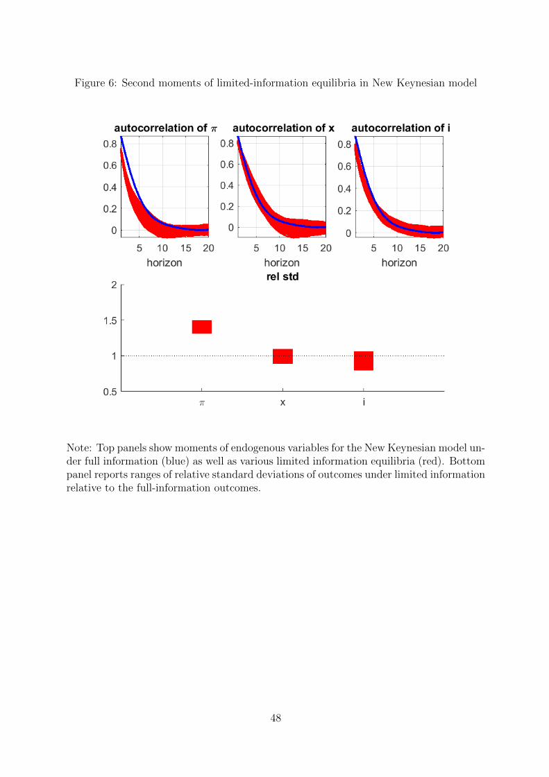
Figure 6: Second moments of limited-information equilibria in New Keynesian model
Note: Top panels show moments of endogenous variables for the New Keynesian model un-der full information (blue) as well as various limited information equilibria (red). Bottompanel reports ranges of relative standard deviations of outcomes under limited informationrelative to the full-information outcomes.
48

FIRE in aggregate data is an important question which is beyond the scope of this paper.
5 Determinate Outcomes Without Optimal Projec-
tion
This section describes an alternative class of policy rules that satisfies the same, if not sim-pler, informational requirements as (60), but also leads to unique equilibrium outcomes.In this alternative class, policy reactions are characterized as responses to incoming data,Zt, instead of responses to optimal projections that are endogenously determined. Ourgeneral framework considers reaction functions for the policy instrument that, as in (60),respond to optimal projections of backward- and forward-looking variables. Rules of thisform could, for example, be motivated by noting that a given rule is deemed desirableunder full information and pointing to a certainty equivalence argument. In fact, basedon reasoning along those lines, Svensson and Woodford (2004) derive optimal reactionsin a form consistent with (60).
A central message of this paper, however, is to note that the interaction of the poli-cymaker’s filtering and private-sector agents’ forward looking behavior, embodied by thelinear difference system in (59), lead to a multiplicity of equilibria that is generally inher-ent in the class of models studied here. Rules of the form in (60) commit the policymakeronly in her responses to projected input variables, but not in her responses to incomingdata. The policymaker’s projections are rational expectations, and the sensitivity of thoseexpectations to incoming data depends on the signal-to-noise ratio of the central bank’sobservables in equilibrium, which results in the potential for multiple equilibria.
We adapt the general environment described in section 3 as follows: Under full in-formation, the policy rule responds only to forward-looking variables and lagged policyinstruments:66
it = Φiit−1 + ΦyY t (108)
An example of such a rule is an outcome-based Taylor rule, while policy rules with stochas-tic intercept are excluded. Forward-looking behavior of the private sector is characterizedby an expectational difference system similar to (59) except that, for simplicity, central-bank projections are assumed to enter (at most) only via the policy rule, that is:
EtSt+1 = ASt +Aiit , (109)
where St continues to denote the stacked vector of backward- and forward-looking vari-ables. As before, we assume the values of the policy-rule coefficients Φi and Φy to be suchthat, when the reaction function (108) is combined with the difference system in (109),there is a unique full-information rational expectations equilibrium.
66We continue to use notation introduced in section 3; policy instruments are denoted it, forward- andbackward-lookign variables, Y t and Xt, and the joint vector of Y t and Xt is St.
49

The measurement vector Zt conveys a noisy signal of every forward-looking variable:67
Zt = Y t + νt νt ∼ N(0,Ωνν) (110)
A policymaker could also consider to simply replace Y t by its noisy signal. That is,the policymaker could set the policy instrument according to:
it = Φiit−1 + Φy (Y t + νt) . (111)
The economy is then described by the expectational difference system (109) and the policyrule (111). Importantly, equilibrium does not hinge on any signal extraction efforts andits determination can be studied using standard methods as described in section 3 3.2.In particular, the only difference between the full-information system consisting of (108)and (109) and the “signal-rule system”, described by (109) and (111), is the presence ofadditional, exogenous driving variables in the form of νt. Both systems share an identicaltransmission of endogenous variables.
Since we assume that the full-information system given by (108) and (109) satisfiesthe conditions for a unique equilibrium, it follows directly that the “signal-rule system”of (109) and (111) also has a unique equilibrium. In particular, using notation introducedabove in our characterization of full-information outcomes for the general case, equilibriumoutcomes have the following form:
Y t = GyxX t + Gyiit−1 + Gyννt (112)
EtX t+1 = PxxX t +Pyiit−1 +Pxννt (113)
where Gyx, Gyi, Pxx, Pyi are conformable partitions of the full-information solution ma-trices P and G, with values identical to (69).68
The ability to achieve equilibrium uniqueness might initially appear to be an attrac-tive feature. However, the dependence of endogenous outcomes on signal noise in (112)and (113) can lead to potentially highly undesirable fluctuations caused by measurementnoise. Effectively, while maintaining the requirement that policy can only respond to ob-servables spanned by Zt, determinacy is achieved under the “signals rule” by committingpolicy to respond to incoming noise with the same sensitivity as it does to Y t. In particu-lar, in the context of the Fisher-example described in section 2, we have Gyν = 0 andX t ispurely exogenous. With this particular configuration, the variance bounds established insection 2 indicates that any admissible equilibrium under the corresponding projections-based policy rule, that is it = Φiit−1 + ΦyY t|t, generates less-variable outcomes, at leastin this particular example.
As described in the Supplementary Appendix, the variance bound derived in the sim-ple example of section 2 also extends to the general case, where we have Var (Y t) ≤
67For simplicity, we continue to assume that νt is serially uncorrelated, though equilibrium uniquenesswill not depend on this property.
68The full-information coefficient matrices known from (69) can be partitioned as follows:
P =
[Pii PixPix Pxx
], and G =
[Gyi GyxGii Gix
]. (114)
50
Gyx Var (X t)G′yx + Var (νt). As a result, the difference between the variance-covariancematrix of outcomes for the forward-looking variables under the projection-based ruleand its counterpart generated by the signal-based rule is positive semi-definite; so thatany quadratic loss function over Y t would at least weakly prefer outcomes under theprojections-based rule.
6 Conclusion
This paper studies the implications of imperfect information for equilibrium determinationin linear dynamic models when differently informed agents interact. We introduce a singledeviation from full information rational expectations: one group of agents is strictly lessinformed than another. By doing so, we differentiate between types of agents that havedifferent information sets, but where each agent forms rational expectations conditionalon available information. The implications of this model structure are stark. We showthat indeterminacy of equilibrium is generic in this environment, even if the correspondingfull information setting implies uniqueness.
More concisely, even a small amount of noise in this environment, despite the bestintentions and optimal filtering of a less informed agent, can produce outcomes wherethere is a sunspot component to economic fluctuations. Our paper thereby contributesto a recent literature on informational frictions in rational expectations models. Specif-ically, we discuss the implications for the conduct of monetary policy in a simple modelof inflation determination and a richer New Keynesian model. In addition to markedlychanging equilibrium outcomes qualitatively, our results show that quantitative differencesto the full information benchmark can be economically significant. Similar to other ap-plications, indeterminacy adds persistence and volatility to economic outcomes. Uniqueto our imperfect information setting is, however, the implication, that the variance ofindeterminacy-induced belief shocks is bounded.
Throughout our analysis, we have maintained the assumption that the policymaker’slimited information set is nested inside the public’s information set, which allows us totreat the private sector as a representative agent. The indeterminacy issues identified byour paper should, however, also extend to richer informational environments as long asthe policymaker cannot perfectly observe forward-looking choice variables of the privatesector. The key condition behind our indeterminacy results is that the policymaker doesnot respond one-for-one to belief shocks of the private sector when forward-looking choicevariables of the private agents are only imperfectly observed by the policymaker.
The findings in this paper suggest various avenues for further investigation. For ex-ample, our framework has strong implications for empirical research: The general modelunder limited information has a state-space representation like any other linear dynamicframework so that a likelihood function can be constructed. The key difference and maincomplication with respect to standard frameworks is that the solution of the model isnot certainty equivalent. Conditional on the Kalman gains the model implies a standardrepresentation, but the gains are equilibrium objects and depend on second moment prop-erties of the solution. This can be taken into account in solution and estimation, albeitat the cost of posing non-trivial computational challenges.69
69An alternative empirical approach would be to assume exogenous and constant gains which could
51

Nevertheless, empirical work can be facilitated by the distinction between actual out-comes and policymaker projections made in our framework. Conditional on the limitedinformation set of the policymaker the model is simply a linear RE model that is unaf-fected by the computational issues in the full model. Data on projections could thereforebe used to estimate the model only over the space of central bank projections, whichwould help sharpen inference for the model parameters.
While we illustrate our framework with examples of monetary policy with an imper-fectly informed central bank, it is not limited to applications in monetary policy. Insection 3 we show that indeterminacy is a generic feature for a general class of economieswhere private-sector behavior is characterized by a set of expectational linear differenceequations, exogenous driving processes are Gaussian, policy is described by a linear rulethat responds to the policymaker’s projections of economic conditions, and the projectionsare rational.
A related issue is the choice of the information set. In our examples, we endowed thecentral bank with specific information sets. Alternatively, one could imagine a scenariowhere the policymaker chooses an optimal information set that minimizes the impactof sunspot shocks and possibly reduces the incidence of multiplicity. This direction hasrelevance for policy as central banks operate in a real-time environment fraught withmeasurement error and regularly face judgment calls on the importance of incoming data.
An important extension should be to look beyond a given class of linear policy rules,as considered here, and model the optimal policy choice for a given set of preferences.Such an exercise could also consider how a desirable policy could be implemented with asuitable policy rule, which requires an analysis of equilibrium selection in the presence ofindeterminacy.
Acknowledgements: We wish to thank seminar audiences at the University of Auck-land, Deutsche Bundesbank, Federal Reserve Bank of Dallas, Federal Reserve Bank of St.Louis, University of Lausanne, Texas A&M University, University of Surrey, as well asparticipants at the 2016 CEF Meetings, the 2016 Federal Reserve Macro System Meetingin Cincinnati, the Fall 2016 NBER Dynamic Equilibrium Models Workshop, the Fall 2016Midwest Macro Conference, the 2017 LAEF Workshop at UC Santa Barbara, the 2017SNDE Conference in Paris, the Workshop on Time-Varying Uncertainty in Macro at theUniversity of St. Andrews, the SCE session at the 2018 ASSA Meetings in Philadel-phia, the HKUST Macro Workshop 2018, the EEA 2018 in Cologne, and the 2019 DNBconference on Uncertainty and Non-linearities. We are also grateful to Zhen Huo, PaulLevine, Giacomo Rondina, and Edouard Schaal, as well as our discussants LeonardoMelosi, Robert Tetlow, Todd Walker, and Mark Weder for very useful comments.
nevertheless deliver insights for policy implications in a non-optimal environment. In addition, alternativeempirical techniques might also be informative such as impulse response function matching that do notnecessarily rely on the full solution of the system.
52

Appendix
A The Steady State Kalman Filter
This section describes details of the steady-state Kalman filter for the innovations statespace (75) and (76) when Assumption 3 holds. Existence of a steady-state Kalman fil-ter relies on finding an ergodic distribution for S∗t (and thus St) with constant secondmoments Σ ≡ Var (S∗t ). When a steady-state filter exists, a constant Kalman gain, Krelates projected innovations of St to innovations in the signal, St|t = KZt with:70
K = Cov(St, Zt
)(Var
(Zt
))−1= (AΣC ′ +BD′) (CΣC ′ +DD′)
−1. (A.1)
The dynamics of S∗t are then characterized by
S∗t+1 = (A−KC) S∗t + (B −KD)wt+1 (A.2)
Existence of a steady-state filter depends on finding a symmetric, positive (semi) definitesolution Σ to the following Riccati equation:
Σ = (A−KC)Σ(A−KC)′ +BB′
= AΣA′ +BB′ − (AΣC ′ +BD′) (CΣC ′ +DD′)−1
(AΣC ′ +BD′)′. (A.3)
Intuitively, the Kalman filter seeks to construct mean-squared error optimal projec-tions St|t that minimize Σ. A necessary condition for the existence of a solution to this
minimization problem is the ability to find at least some gain K for which A− KC isstable; otherwise, S∗ would have unstable dynamics as can be seen from (A.2). Thus,existence of the second moment for the residuals, Var (S∗t ) = Σ ≥ 0, is synonymous witha stable transition matrix A−KC.
Formal conditions for the existence of a time-invariant Kalman filter have been stated,among others, by Anderson and Moore (1979), Anderson, McGrattan, Hansen and Sargent(1996), Kailath, Sayed and Hassibi (2000), and Hansen and Sargent (2007). Necessaryand sufficient conditions for the existence of a unique and stabilizing solution that is alsopositive semi-definite depend on the “detectability” and “unit-circle controllability” ofcertain matrices in our state space. We restate those concepts next.
Definition 3 (Detectability). A pair of matrices (A,C) is detectable when no righteigenvector of A that is associated with an unstable eigenvalue is orthogonal to the rowspace of C. That is, there is no non-zero column vector v such that Av = vλ and |λ| ≥ 1with Cv = 0.
Detectability alone is already sufficient for the existence of some solution to the Riccatiequation such that A −KC is stable; see (Kailath et al. 2000, Table E.1). Evidently,detectability is assured when A is a stable matrix, regardless of C. To gain furtherintuition for the role of detectability, consider transforming St into “canonical variables”
70See also equation (78) in the paper.
53

by premultiplying St with the matrix of eigenvectors of A — this transformation intocanonical variables is at the heart of procedures for solving rational expectations modelsknown from Blanchard and Kahn (1980), King and Watson (1998), Klein (2000), Sims(2002). Detectability then requires the signal equation (76) to provide some signal (i.e.to have non-zero loadings) for any unstable canonical variables.71
To establish existence of a solution to the Riccati equation that is unique and positivesemi-definite, we follow Kailath et al. (2000) and require unit-circle controllability, definedas follows.
Definition 4 (Unit-circle controllability). The pair (A,B) is unit-circle controllable whenno left-eigenvector of A associated with an eigenvalue on the unit circle is orthogonal tothe column space of B. That is, there is no non-zero row vector v such that vA = vλwith |λ| = 1 and vB = 0.
In our state space, with BD′ 6= 0, shocks to state and measurement equation aregenerally correlated. Unit-circle controllability is thus applied to the following transfor-mations of A, B:72
AC ≡ A−BD′ (DD′)−1C BC ≡ B
(I −D′ (DD′)
−1D)
(A.4)
Based on these definitions, the following theorem restates results from Kailath et al.(2000) in our notation:
Theorem 3 (Stabilizing Solution to Riccati Equation). Provided Assumption 3 holds,a stabilizing and positive semi-definite solution to the Riccati equation (A.3) exists when(AC ,BC) is unit-circle controllable and (A,C) is detectable. The steady-state KalmanK gain is such that A−KC is a stable matrix, and the stabilizing solution is unique.73
Proof. See Theorem E.5.1 of Kailath et al. (2000); related results are also presented inAnderson et al. (1996), or Chapter 4 of Anderson and Moore (1979).
In our context, with C = HA and D = HB, the conditions for detectability andunit-circle controllability can also be restated as follows.
Proposition 7 (Detectability of (A,H)). With C = HA, detectability of (A,C) isequivalent to detectability of (A,H)
Proof. When (A,C) are detectable, we have Cv 6= 0 for any right-eigenvector of Aassociated with an eigenvalue λ on or outside the unit circle, |λ| ≥ 1. With C = HA wethen also have Cv = HAv = Hvλ 6= 0⇔Hv 6= 0
71Specifically, let A = V ΛV −1 with Λ diagonal be the eigenvalue-eigenvector factorization of A sothat the columns of V correspond to the right eigenvectors ofA. Define canonical variables SCt ≡ V
−1St.The signal equation can then be stated as Zt = CV SCt and detectability requires the signal equation tohave non-zero loadings on at least every canonical variable associated with an unstable eigenvalue in Λ.
72Notice thatBC = BMD whereMD = I−D′ (DD′)−1D is a projection matrix, which is symmetric
and idempotent,MD =MDMD, and orthogonal to the row space of D.To appreciate the role ofMD,consider the following thought experiment: MD construct the residual in projecting the shocks of thesystem off the shocks in the signal equation, wt − E(wt|Dwt) =MDwt.
73There may be other, non-stabilizing positive semi-definite solutions.
54

Furthermore, with C = HA and D = HB, the above expressions for AC and BC
can be transformed as follows:
AC = (I − P C)A and BC = (I − P C)B with P C ≡ BH ′ (HBB′H ′)−1H .(A.5)
P C is a non-symmetric, idempotent projection matrix with HP C = H .74
Proposition 8 (Unit-circle controllability of (A(I − P C),B)). With C = HA andD = HB, unit-circle controllability of (AC ,BC) is equivalent to unit-circle controllabilityof (A(I − P C),B) with P C defined in (A.5).
Proof. Suppose (AC ,BC) are unit-circle controllable. Let v ≡ v(I − P C) and note thatleft-eigenvectors ofAC associated with eigenvalues on the unit circle cannot be orthogonalto P C (otherwise we would have vAC = 0). Accordingly, vAC = vλ with |λ| = 1,vBC 6= 0 and v 6= 0 is equivalent to vA(I − P C) = vλ with |λ| = 1, v 6= 0 vB 6= 0.The converse reasoning applies as well.
As discussed in the main text, an upshot of Proposition 8 is that a sufficient conditionfor unit-circle controllability of (AC ,BC) is for B to have full rank.
Finally, for convenience, we define the the joint concept of detectability and unit-circlecontrollability for the triplet (A,B,H).
Definition 5 (Joint detectability and unit-circle controllability). The triplet A,B,H isdetectable and unit-circle controllable when (A,H) is detectable and (A(I −P C),B) isunit-circle controllable, where P C is defined in (A.5).
B Endogenous Forecast Errors when the Signal is
Endogenous
This section of the appendix describes an algorithm to solve numerically for the en-dogenous forecast errors in the endogenous-signal case of our general setup, described insection 3. Our numerical approach combines elements of standard techniques for solvinglinear RE models with a fast algorithm to solve the non-linear fixed-point problem forthe Riccati-equation embedded in the Kalman-filter while ensuring consistency with theprojection condition. The algorithm searches for shock loadings Γηε and Γηb that satisfythe projection condition for a Kalman filter that is consistent with equilibrium outcomesof endogenous and exogenous variables.
As described in section 3, the endogenous-signal case considers a measurement equa-tion of the form
Zt = HxX t + Y t . (87)
74An idempotent matrix is equal to its own square, that is PC = PCPC , and the eigenvalues of anidempotent matrix are either zero or one and we have |PC | = 0.
55

By construction, we have Zt = Zt|t and thus Y ∗t = −HxX∗t , so that the innovation
system given by (75) and (76) can then be simplified as follows:
X t+1 = AX∗t + Bwt+1 (B.1)
Zt+1 = CX∗t + Dwt+1 (B.2)
with A = Axx −AxyHx (B.3)
B =[Bxε 0
](B.4)
C = Hx (Axx −AxyHx) +Ayx −AyyHx (B.5)
D =[(HxBxε + Γηε) Γηb
](B.6)
where Axx, Axy, etc. denote suitable sub-matrices of A; and D embodies a given guessof Γηε and Γηb.
For a given D, the Kalman-filtering solution to this system generates a Kalman gainKx which can be used to form projections X t|t = KxZt. What remains to be seen is
whether this guess for D also satisfies the projection condition. The projection conditionrequires Ky = GyxKx. Together with the projection condition, the measurement equa-tion (87) implies I = HxKx + Ky = (Hx + Gyx)Kx. All told, we need to find shockloadings that support a gain Kx such that LKx = I where L = Hx + Gyx.
We employ a numerical solver that searches for a D that generates a Kalman gainKx such that LKx = I. Given a solution for D that satisfies the projection conditionLKx = I, we can then back out Γε and Γb based on (B.6).
References
Acharya, S., Benhabib, J. and Huo, Z.: 2017, The anatomy of sentiment-driven fluctua-tions, NBER Working Papers 23136, National Bureau of Economic Research, Inc.
Anderson, B. D. O. and Moore, J. B.: 1979, Optimal Filtering, Information and SystemSciences Series, Prentice-Hall Inc., Englewood Cliffs, New Jersey.
Anderson, E. W., McGrattan, E. R., Hansen, L. P. and Sargent, T. J.: 1996, Mechanics offorming and estimating dynamic linear economies, in H. M. Amman, D. A. Kendrickand J. Rust (eds), Handbook of Computational Economics, Vol. 1, Elsevier, chapter 4,pp. 171–252.
Angeletos, G. and La’O, J.: 2013, Sentiments, Econometrica 81(2), 739–779.
Aoki, K.: 2006, Optimal commitment policy under noisy information, Journal of Eco-nomic Dynamics and Control 30(1), 81–109.
Ascari, G., Bonomolo, P. and Lopes, H. F.: 2019, Walk on the wild side: Temporarily un-stable paths and multiplicative sunspots, American Economic Review 109(5), 1805–42.
56

Baxter, B., Graham, L. and Wright, S.: 2011, Invertible and non-invertible informationsets in linear rational expectations models, Journal of Economic Dynamics and Con-trol 35(3), 295–311.
Blanchard, O. J.: 1979, Backward and forward solutions for economies with rationalexpectations, The American Economic Review 69(2), 114–118.
Benhabib, J. and Farmer, R.: 1994, Indeterminacy and increasing returns, Journal ofEconomic Theory 63(1), 19–41.
Benhabib, J., Wang, P. and Wen, Y.: 2015, Sentiments and Aggregate Demand Fluctua-tions, Econometrica 83, 549–585.
Bernanke, B. S. and Woodford, M.: 1997, Inflation forecasts and monetary policy, Journalof Money, Credit and Banking 29(4), 653–684.
Blanchard, O. J. and Kahn, C. M.: 1980, The solution of linear difference models underrational expectations, Econometrica 48(5), 1305–1312.
Bullard, J. and Mitra, K.: 2002, Learning about monetary policy rules, Journal of Mon-etary Economics 49, 1105–1129.
Carboni, G. and Ellison, M.: 2011, Inflation and output volatility under asymmetricincomplete information, Journal of Economic Dynamics and Control 35(1), 40–51.
Clarida, R., Gali, J. and Gertler, M.: 2000, Monetary policy rules and macroeconomic sta-bility: Evidence and some theory, The Quarterly Journal of Economics 115(1), 147–180.
Dotsey, M. and Hornstein, A.: 2003, Should a monetary policymaker look at money?,Journal of Monetary Economics 50(3), 547–579.
Evans, G. W. and Honkapohja, S.: 2001, Learning and Expectations in Marcoeconomics,Princeton University Press, Princeton, NJ.
Evans, G. W. and McGough, B.: 2005, Stable sunspot solutions in models with predeter-mined variables, Journal of Economic Dynamics and Control 29(4), 601–625.
Farmer, R. and Guo, J.-T.: 1994, Real business cycles and the animal spirits hypothesis,Journal of Economic Theory 63(1), 42–72.
Farmer, R., Khramov, V. and Nicolo, G.: 2015, Solving and estimating indeterminateDSGE models, Journal of Economic Dynamics and Control 54, 17–36.
Faust, J. and Svensson, L. E. O.: 2002, The equilibrium degree of transparency andcontrol in monetary policy, Journal of Money, Credit and Banking 34(2), 520–39.
Fernandez-Villaverde, J., Rubio-Ramırez, J. F., Sargent, T. J. and Watson, M. W.: 2007,ABCs (and Ds) of understanding VARs, American Economic Review 97(3), 1021–1026.
57

Goodhart, C.: 1987, Problems of monetary management: The U.K. experience, in A. S.Courakis (ed.), Inflation, Depression, and Economic Policy in the West, Barnes &Noble Books, New Jersey, pp. 111–146.
Hansen, L. P. and Sargent, T. J.: 2007, Robustness, Princeton University Press.
Kailath, T., Sayed, A. H. and Hassibi, B.: 2000, Linear Estimation, Prentice Hall Infor-mation and System Sciences Series, Pearson Publishing.
King, R. G. and Watson, M. W.: 1998, The solution of singular linear difference systemsunder rational expectations, International Economic Review 39(4), 1015–1026.
Klein, P.: 2000, Using the generalized Schur form to solve a multivariate linear rationalexpectations model, Journal of Economic Dynamics and Control 24(10), 1405–1423.
Laubach, T. and Williams, J. C.: 2003, Measuring the natural rate of interest, The Reviewof Economics and Statistics 85(4), 1063–1070.
Lubik, T. A. and Matthes, C.: 2016, Indeterminacy and learning: An analysis of monetarypolicy in the great inflation, Journal of Monetary Economics 82(C), 85–106.
Lubik, T. A. and Schorfheide, F.: 2003, Computing sunspot equilibria in linear rationalexpectations models, Journal of Economic Dynamics and Control 28(2), 273–285.
Lubik, T. A. and Schorfheide, F.: 2004, Testing for indeterminacy: An application toU.S. monetary policy, The American Economic Review 94(1), 190–217.
Mertens, E.: 2016, Managing beliefs about monetary policy under discretion, Journal ofMoney, Credit and Banking 48(4), 661–698.
Morris, S. and Shin, H. S.: 2018, Central bank forward guidance and the signal value ofmarket prices, AEA Papers and Proceedings 108, 572–577.
Nimark, K.: 2008a, Dynamic pricing and imperfect common knowledge, Journal of Mon-etary Economics 55(2), 365–382.
Nimark, K.: 2008b, Monetary policy with signal extraction from the bond market, Journalof Monetary Economics 55(8), 1389–1400.
Nimark, K. P.: 2014, Man-bites-dog business cycles, American Economic Review104(8), 2320–2367.
Orphanides, A.: 2001, Monetary policy rules based on real-time data, American EconomicReview 91(4), 964–985.
Orphanides, A.: 2003, Monetary policy evaluation with noisy information, Journal ofMonetary Economics 50(3), 605–631. Swiss National Bank/Study Center GerzenseeConference on Monetary Policy under Incomplete Information.
Orphanides, A. and Williams, J. C.: 2006, Monetary policy with imperfect knowledge,Journal of the European Economic Association 4(2-3), 366–375.
58

Orphanides, A. and Williams, J. C.: 2007, Robust monetary policy with imperfect knowl-edge, Journal of Monetary Economics 54(5), 1406–1435.
Rondina, G. and Walker, T.: 2017, Confounding dynamics. mimeo.
Sargent, T. J.: 1991, Equilibrium with signal extraction from endogenous variables, Jour-nal of Economic Dynamics and Control 15(2), 245–273.
Schmitt-Grohe, S.: 1997, Comparing four models of aggregate fluctuations due to self-fulfilling expectations, Journal of Economic Theory 72(1), 96–147.
Siemroth, C.: 2019, The informational content of prices when policy makers react tofinancial markets, Journal of Economic Theory 179(C), 240–274.
Sims, C. A.: 2002, Solving linear rational expectations models, Computational Economics20(1-2), 1–20.
Svensson, L. E. O. and Woodford, M.: 2004, Indicator variables for optimal policy underasymmetric information, Journal of Economic Dynamics and Control 28(4), 661–690.
Taylor, J. B.: 1977, Conditions for unique solutions in stochastic macroeconomic modelswith rational expectations, Econometrica 45(6), 1377–1385.
Woodford, M.: 2003, Interest and Prices, Princeton University Press, Princeton, NJ.
59