Index Notation in Mathematics and Modelling

Language LPL: Theory and Exercises

Tony Hürlimann

August 25, 2017

Abstract

This paper explains indexing notation in mathematics and its implementation

in the modeling language LPL. Indexing is one of the most fundamental concept in

mathematical notation. It is extremely powerful and allows the modeler to concisely

formulate a complex mathematical model. A certain number of exercises are given

and implemented in LPL to test the concepts.

1

Contents

1 Introduction 3

2 De�nitions and Notations 52.1 Exercises in the Sigma Notation . . . . . . . . . . . . . . . . . . . . . . . . 52.2 Formal De�nition . . . . . . . . . . . . . . . . . . . . . . . . . . . . . . . . 72.3 Extensions . . . . . . . . . . . . . . . . . . . . . . . . . . . . . . . . . . . . 10

2.3.1 A list of (indexed) expressions . . . . . . . . . . . . . . . . . . . . . 102.3.2 Index Sets as Expressions . . . . . . . . . . . . . . . . . . . . . . . 112.3.3 Compound Index Notation . . . . . . . . . . . . . . . . . . . . . . . 122.3.4 Indexed index sets . . . . . . . . . . . . . . . . . . . . . . . . . . . 162.3.5 Ordering . . . . . . . . . . . . . . . . . . . . . . . . . . . . . . . . . 16

3 Index Notation in LPL 17

4 A Complete Problem: Exercise 2 21

5 Data for Exercise 2 23

6 An Optimizing Problem Version 246.1 Version 1: the easy problem . . . . . . . . . . . . . . . . . . . . . . . . . . 256.2 Version 2: Limit Capacity . . . . . . . . . . . . . . . . . . . . . . . . . . . 276.3 Version 3: with Setup Costs . . . . . . . . . . . . . . . . . . . . . . . . . . 29

7 Conclusion 30

2

1 Introduction

To work with a mass of data, a concise formalism and notation is needed. In mathematics,the so-called indexed notation. This notation is an integral and fundamental part ofevery mathematical modeling activity � and they are also used in mathematical modelinglanguages as in LPL [3] � to group various objects and entities. It is surprising howlittle has been published in the community of modeling language design on this concept.Even in mathematical textbooks, the indexed notation used in formulae is often takenfor granted and not much thought is given to it1. This fact contrasts with my experiencethat students often have di�culties with the indexed notation in mathematics.

To represent single data, called scalars, names and expressions are used, such as:

x, y or x− y

To specify further what we mean by a symbol, we write x, y ∈ IR, for example, sayingthat x and y represent any real numbers. We can attach a new symbol (z) to an expressionas in:

z = x− y

meaning that z is a new number which is de�ned as the di�erence of x and y. We say�z substitutes the expression x− y�. In this way, we can build complex expressions. Welearnt this algebraic notation already in school. These symbols have no speci�c �meaning�besides the fact that they represent numbers. To use them in a modeling context, we thenattach a meaning. For example, in an economical context we might interpret �x� as �totalrevenue� and �y� as �total costs�. Then �z� might be interpreted as �total pro�t�. Thereis nothing magic about these symbols, instead of writing z = x− y we can also write:

total pro�t = total revenue− total costs

However, to economize our writings we prefer short �names�. But there is nothing wrongwith longer names to make expressions more readable in a speci�c context.

It seems to be a little bit less familiar that in the same way as using symbols forscalars, symbols can represent mass of data. Suppose that we want to express the pro�tof several pro�t centers in a company. Then we could write:

pro�t at center 1 = revenue at center 1− costs at center 1

pro�t at center 2 = revenue at center 2− costs at center 2

pro�t at center 3 = revenue at center 3− costs at center 3

. . . etc. . . .

or

z1 = x1− y1

z2 = x2− y2

1A notable exception is [1], which devotes the whole Chapter 2 to indexed expressions and their usein mathematics.

3

z3 = x3− y3

. . . etc. . . .

The �etc.� means that we have to continue writing as many lines as we have pro�t centers� a rather boring task!

There is, however, a much more economical way in mathematics to represent all theseexpressions in a single statement. It is the indexed notation. To formulate them, we �rstintroduce a set: the set I of all pro�t centers:

I = {center 1 , center 2 , . . . }

here again the � . . .� means that we continue writing all centers in a list. Often a shortname form is used as follows:

I = {1 . . . n} where n ∈ IN+

In the previous set de�nition we just mean that there are n centers, n being a positivenumber. We are not concerned right now of how many centers there are, we just say �n�� it can be 5 or 1000. Of course, in a concrete context we must specify the number n, butit is part of the data of that speci�c context.

In a second step, we introduce symbols for all pro�ts, revenues and costs. Now, insteadof using each time a new symbol, we just attach an subscript to the symbols: zi, xi, yi toexpress the fact that they �mean� the pro�t, the revenue and the cost of the i-th center,together with the notation i ∈ I, which means that i just designates an arbitrary (i-th)element in I. Hence, All data can be written in a concise way as follows:

xi, yi, zi where i ∈ I

Mathematically speaking,three vectors to represent all data are declared. The list ofexpression then can be written in a single statement as follows:

zi = xi − yi with i ∈ I

This notation is in fact nothing else than an economical way of the following n expressions:

z1 = x1 − y1

z2 = x2 − y2

. . .

zn = xn − yn

where n is some positive integer.

In a similar way, we can concisely build an expression that sums all pro�ts, for instance.For this purpose we use the mathematical operator

∑. The total pro�t p of all pro�t

centers can be formulated as follows:

p =∑i∈I

zi

After this introductory example, this paper presents now a more precise way, on howthe indexed notation is de�ned and how it can be used.

4

2 De�nitions and Notations

Index sets are essential for mastering the complexity of large models. All elements in amodel, such as variables, parameters, and constraints � as will be shown later on � canappear in groups, in the same way they are indexed in mathematical notation.

The convention in algebraic notation to denote a set of similar expressions is to useindexes and index sets. For example, a summation of n (numerical) terms

a1 + a2 + · · ·+ an−1 + an (1)

is commonly abbreviated using the notation

n∑i=1

ai (2)

The expression (1) is called three-dots notation and expression (2) is called sigma-notation. Both expression are equivalent, but (2) is much shorter and more general. Thelater was introduced by Joseph Fourier in 1820, according to [1, p. 22]. There existdi�erent variants of expression (2) :

∑1≤i≤n

ai ,n∑

i=1

ai ,∑

i∈{1...n}

ai ,∑i∈I

ai with I = {1 . . . n} (3)

All four expressions in (3) are equivalent and they have all their advantages anddisadvantages. The last notation in (3) is more general, because the index set I can bean arbitrary set de�ned outside the summation expression.

2.1 Exercises in the Sigma Notation

Before we generalize the indexed notation, let us give some examples with the sigma form.A notation

∑5i=1 xi means that i is replaced by whole numbers starting with 1 until

the number 5 is reached. Thus

4∑i=2

xi = x2 + x3 + x4

and

5∑i=2

xi = x2 + x3 + x4 + x5

Hence, the notation∑n

i=1 tells us:1. to add the numbers xi,

2. to start with i = 1, that is, with x1,3. to stop with i = n, that is, with xn (where n is some positive integer).

As an example, let us assign the following values: x1 = 10, x2 = 8, x3 = 2, x4 = 15, andx5 = 22. Then we have:

5

5∑i=1

xi = x1 + x2 + x3 + x4 + x5 = 10 + 8 + 2 + 15 + 22 = 57

The name i is a dummy variable, any other name could be used. We could have used j,the expression would have be exactly the same, hence:

5∑i=1

xi =5∑

j=1

xj

Now let us �nd∑4

i=1 3xi based on the previous values. Again we start with i = 1 and wereplace 3xi with its value:

4∑i=1

3xi = 3x1 + 3x2 + 3x3 + 3x4 = 3 · 10 + 3 · 8 + 3 · 2 + 3 · 15 = 105

Similarly, let use �nd∑5

i=2(xi − 8): This is:

5∑i=2

(xi − 8) = (x2 − 8) + (x3 − 8) + (x4 − 8) + (x5 − 8)

= (8− 8) + (2− 8) + (15− 8) + (22− 8) = 17

One should be careful with the parentheses. The expression∑5

i=2(xi− 8) is not the sameas∑5

i=2 xi − 8. The later evaluates to (the 8 is not included in the sum):

5∑i=2

xi − 8 = x2 + x3 + x4 + x5 − 8 = 29

We also use sigma notation in the following way:

4∑j=1

j2 = 12 + 22 + 32 + 42 = 30

The same principle applies here. j is replaced in the expression j2 by numbers startingwith 1 and ending with 4, and then adding up all four terms.

6

For the sigma notation we have three important transformation rules:

Rule 1: if c is a constant, then:

n∑i=1

cxi = cn∑

i=1

xi

Rule 2: if c is a constant, then:

n∑i=1

c = nc

Rule 3: Adding the term can be distributed:

< qquad

n∑i=1

(xi + yi) =n∑

i=1

xi +n∑

i=1

yi

Proof:

n∑i=1

cxi = cx1 + cx2 + . . .+ cxn−1 + cxn

= c · (x1 + x2 + . . .+ xn−1 + xn) = c ·n∑

i=1

xi

n∑i=1

c = c+ c+ . . .+ c︸ ︷︷ ︸n−times

= n× c = nc

n∑i=1

(xi + yi) = (x1 + y1) + . . .+ (xn + yn)

= (x1 + . . .+ xn) + (y1 + . . .+ yn) =n∑

i=1

xi +n∑

i=1

yi

End of proof

2.2 Formal De�nition

More formally, let us call an indexed notation written as⊙i∈I

Ei (4)

a formal expression containing the following elements:

1. An index operator, here written as⊙

. This operator can be any associative andcommutative operator, such as

∑(summation), for example.

7

2. An index set, represented by I, being any countable (�nite or in�nite) collection ofelements. The elements can be any indivisible item. Often they are integers.

3. An active index i (in i ∈ I), attached to the index operator.

4. An indexed expression Ei, that normally contains the same index name again. Wecall this index passive index. The reason for that will be clear later on.

(1) The index operator: It is clear why the index operator must be commutative andassociative: A mathematical set is unordered and its elements can be �traversed� in anyorder. As an example, the

∑does not specify in which order the indexed expressions Ei

are added up. Various operators ful�ll these requirements. Besides the addition, repre-sented by the operator

∑, the following index operators are commonly used (examples

will be given later on):

• The product (multiplication)∏

: The indexed expressions are multiplied.

• The Max (Min) operator, written asmaxi∈I (mini∈I): They return the largest (small-est) indexed expression in the list.

• In Boolean logical expressions we use the AND- and OR-operators (∧,∨): They

check whether all indexed expressions are true or at least one is true.

• An particular index operator is the list operator.∧. It is used to list indexed expres-

sions.

(2) The index set: In the simplest case, the elements of the index set are integers,a s in

I = {1, . . . , n}, where n > 0

However, they can also be identi�ers (symbolic names), strings or any other items andeven sets representing elements of a set. In the following index set I with:

I = { spring , summer , autumn , winter }

the four elements are identi�ers. Sets are unordered as mentioned above. In modelingenvironments, however, we often must impose a speci�c order, for example, if a set consistsof a number of time periods or time points. Then the natural order is the sequence ofthese periods. For example, the weekdays:

I = { Mon, Tue, Wen , Thu, Fri, Sat, Son }

The order is important in such a context, because we often need to refer to the �pre-vious�, the �next�, the �last� or the ��rst� period in an indexed expression. In spacial ar-rangements the order might also be important. Consider a chessboard with I = {1 . . . 8}rows and columns, then it makes sense to refer to the �neighbor� columns at the left orright and the �neighbor� rows above or below a given cell. In another context, the order-ing might have a semantical meaning. For example, if we want � for a speci�c purpose� impose an order on a list of products. We can order the product by �importance� orwhatever criterion we need. Without ordering the statement to generate a �list with the

8

�rst 10 products� would have no meaning. Without any externally imposed criterion theordering of the products would have no meaning, as in:

I = { bred, cheese, meat, eggs }

We also may have set of tuples, which is extremely common in modeling. An exampleis the list of all positive integer grid points in a Euclidean space:

I = {(x, y) | x, y ∈ IN+}

= {(0, 0), (1, 0), (1, 1), (0, 1), (0, 2), (1, 2), (2, 2), (2, 1), . . .}

Another important case in modeling is �set of sets�. As a concrete example, certainclients are served from certain warehouses. Let I = {1, . . .m} be a set of warehouses andlet J = {1, . . . n} be a set of clients, then the set S:

S = {Qi | i ∈ I , Qi ⊆ J}

tells us which client j is served from which warehouse. Example:

S = {{1, 2, 3}, {2, 3}, {}, {2}} , hence

Q1 = {1, 2, 3}Q2 = {2, 3}Q3 = {}Q4 = {2}

says, that warehouse 1 serves client 1, 2, 3, warehouse 2 serves clients 2, 3, warehouse 3do not serve any client, and warehouse 4 serves client 2, that is, Qj is the set of clientsserved by warehouse j ∈ J . Note that often this kind of data can also be formulated asa tuple list:

Si,j = {(1, 1), (1, 2), (1, 3), (2, 2), (2, 3), (4, 2)} ∀ i ∈ I, j ∈ J

(3) The active index: The active index is a (dummy) name (or an identi�er) repre-senting an arbitrary element in the index set. The passive index is also an identi�er usedin the indexed expression which must have the same spelling as the active index. Theterm i ∈ I, consisting of the active index and the index set, is called an indexing term.The active index and the passive index are used as place-holders to de�ne a bijectivemapping between the index set and a set of indexed expressions. Each element i in theindex set maps to an indexed expression by replacing the passive index with the corre-sponding element i in the index set. This mapping is called the index mechanism. In fact,

it de�nes the (bijective) function f : if−→ Ei with i ∈ I. This mapping supposes that

the corresponding indexed expressions Ei exist. The domain of this function f containsthe elements of the index set {1, 2, . . . , n}, and the codomain (or the range) is the set ofindexed expressions {E1, E2, . . . , En}.

(4) The index expression: The indexed expression is an arbitrary expression. It is notnecessary that it contains a passive index. For example, in the expression:∑

i∈I

3 with I = {1 . . . n}

9

the indexed expression is just 3. The whole expression then reduces simply to:

3 + 3 + . . .+ 3︸ ︷︷ ︸n−times

= 3 · n

The indexed expression can alas be reduced to a passive index as in:∑i∈I

i with I = {1 . . . n}

in which case the indexed expression is just i. The whole expression reduces to:

1 + 2 + . . .+ n

The indexed expression can itself contain index operators. For example:

∑i∈I

(∑j∈J

Fi,j

)with I = {1 . . . n}, J = {1 . . .m}

In this case, the expression �rst expands to:∑i∈I

(Fi,1 + Fi,2 + . . .+ Fi,m) with I = {1 . . . n}

Finally, the outer sum is applied to get the expression

F1,1 + F1,2 + . . .+ F1,m + F2,1 + F2,2 + . . . . . .+ Fn,m

De�nition: An indexed notation is a formula expressing the fact that the index operator

is applied to the set of indexed expressions constructed by the index mechanism., that is,

a bijective mapping between the elements of the index set and the indexed expressions.

2.3 Extensions

The general indexed notation is given by the following notation as seen before:⊙i∈I

Ei

This is really the most general notation, no further concepts are needed to write morecomplex index notations. This will be shown now by studying several �extensions�, whichall can be reduced to this simple form.

2.3.1 A list of (indexed) expressions

A list of expressions is normally written as follows:

zi = xi − yi with i ∈ I

This notation is very common. It says that the equations zi = xi − yi has to be repeatedas many times as I has elements. However, this notation could be transformed into thegeneral indexed notation by using the list operator as follows:

10

.∧i∈I

(zi = xi − yi)

The index operator is the.∧-operator. The meaning of this operator is to list all indexed

expressions. In this case, the indexed expression is normally an equation or an assignment,hence the �side e�ect� of this operator is to assign a list of values. Of course, in amathematical text we would prefer the �rst notation, because it is so common. However,this example shows that it can really be seen as an indexed notation. This fact will beimportant in the context of modeling languages later on, because we can use the samesyntax to specify a list of expressions. To express it, we only need to use the list operatorinstead of any other index operator, as for instance the sigma operator.

2.3.2 Index Sets as Expressions

In many situations, the index set is not simply an explicit list of elements, as in I ={1 . . . n}. Of course, any set expression can be used to construct the index set I. Hence,I could be the union or the intersection of other sets as in the following expression:

I = J ∪K or I = J ∩K

This kind of modi�cation does not change anything for the indexed notation. It is imma-terial, how the index set is constructed. Sometimes, however, we construct I as a subsetof another set, say J , such that I ⊆ J , and we use the notation:

I = {j ∈ J | P (j)}where P (j) is a property about j ∈ J that is either true or false. The notation means:�for all j ∈ J such that P (j) is true�. Clearly, if P (j) is true for all elements in J thenthe two sets are equal (I = J). However, normally P (j) expresses a property that is trueonly for a proper subset of J . Using I in an indexed notation, we could write:∑

i∈I

Ei with I = {j ∈ J | P (j)}

However, it is more common and much shorter to use the notation which is as follows:∑j∈J |P (j)

Ej

Hence, we attach the property P (j) directly to the indexing term starting it with thesymbol |. This is extremely useful and very common in modeling. Suppose we have alist of products. Then it is very common to sum over di�erent subsets of products, forinstance �all products for which the demand is larger than x� or �all products that aregreen� or whatever. It would be exaggerated to generate an explicit named index set eachtime.

We give several examples: Suppose we have x1 = 10, x2 = 8, x3 = 2, x4 = 15, andx5 = 22. Furthermore, P (i) is de�ned to be �xi ≤ 9�, and Q(i) is de�ned as �i ≥ 4� withi ∈ I = {1 . . . 5}. Then we evaluate the following expressions:∑

i∈I|P (i)

xi = x2 + x3 = 8 + 2 = 10

11

∑i∈I|Q(i)

xi = x4 + x5 = 15 + 22 = 37

In the �rst expression P (i) is true only for x2 and x3, hence the sum take place only overthese two terms. In the second expression, Q(i) is true only for i = 4 and i = 5.

There is no need to explicitly name the properties; their corresponding expressionscould be directly used in the indexing terms. Hence the two previous expressions couldalso be written as: ∑

i∈I|xi≤9

xi = x2 + x3 = 8 + 2 = 10

∑i∈I|i≥4

x1 = x4 + x5 = 15 + 22 = 37

We can write any Boolean expression after | . . . in the indexing term. This expression iscalled indexing condition.

Other examples with k ∈ K = {1 . . . 100} are as following:

∑k∈K|k2≤100

k =∑

i∈{1...10}

i = 1 + 2 + . . .+ 10

∑k∈K|3≤k≤5

k2 = 32 + 42 + 52 = 50

∑k∈K|k is prime

k = 2 + 3 + 5 + 7 + 11 + 17 + ...+ 97

In the �rst expression k2 ≤ 100 is only true for 1 ≤ k ≤ 10. In the second expression,only 3, 4, 5 are allow for k. In the third, we say to take every k up to 100, such that k isprime.We saw, to extend the indexing term from �i ∈ I� to �i ∈ I | P (i)� does not changethe meaning of the indexed notation. The expression i ∈ I | P (i) is still a set albeit asubset of I that has no explicit name. However, no further concept has been added tothe indexed notation.

2.3.3 Compound Index Notation

An indexed expression can itself contain an indexed notation, which generates nestedindexed notations, as in the following expression:

⊙i∈I

(⊗j∈J

Fi,j

)(5)

where⊙

and⊗

are two arbitrary index operators. If the two operators are di�erentthen we need to evaluate the inner expression �rst and the outer afterwards. A notableexample is a system of m linear equations with n variables that is commonly noted asfollows: ∑

j∈{1...n}

ai,jxj = bi with i ∈ {1 . . .m}

12

Using the list operator.∧, these formula can be noted as a nested indexed notation, that

is, a notation where the index expression contains itself an indexed notation, with the

outer index operator.∧and the inner index operator as

∑. The nested notation then is

noted as follows:

.∧i∈{1...m}

∑j∈{1...n}

ai,jxj = bi

This notation is a very short writing of the following system of equations:

a1,1x1 + a1,2x2 + . . .+ a1,n−1xn−1 + a1,nxn = b1

a2,1x1 + a2,2x2 + . . .+ a2,n−1xn−1 + a2,nxn = b2

. . . = . . .

am,1x1 + am,2x2 + . . .+ am,n−1xn−1 + am,nxn = bm

On the other hand, if both index operators in (5) are identical, then the two indexoperators can be merged in the following way:

⊙i∈I

(⊙j∈J

Fi,j

)=

⊙i∈I, j∈J

Fi,j

It means that we merge the operator and unify also the indexing terms to be written as�i ∈ I, j ∈ J�. It signi�es that we build every tuple of the Cartesian Product of the twosets: (i, j) ∈ I × J . As an example, suppose I = {1, 2} and J = {a, b, c} then the indexset is I × J = {(1, a), (1, b), (1, c), ((2, a), (2, b), (2, c)} � it consists of 6 tuples. There aretwo active indexes i and j, or a tuple (i, j) of active indexes. Hence we also may writethis in the following way: ⊙

(i,j)∈I×J

Fi,j

where the index set is I × J and the active index is replaced by the notation (i, j) whichis called an active index tuple. In this case, the names within the active index tuples arecalled active indices. The active indices are now place-holders for the single componentsof the tuple.

The index set I × J is also a set, the set of all tuples in the Cartesian Product. Henceif we do not need to access the single components within the product, we can replace (i, j)by a single active index, say k, and I × J can be replaced by a set name, say K. Now wesee that the previous formula really reduces to our general indexed notation, which is asfollows: ⊙

(i,j)∈I×J

Fi,j =⊙k∈K

Ek

Since indexed notation with multiple indexing terms really is reducible to indexed notationwith one indexing term, we only need to extend the de�nition of index sets:

13

De�nition: A compound index set is any countable (�nite or in�nite) collection of elements,

where all elements are either indivisible items called atoms or tuples containing all the same

number of components.

It is interesting to note that the previous three indexed notations are essentially the same.In addition they allows one to specify a proper subset of the full Cartesian Product.

Sometimes access to the tuple itself and to its components is needed. In such cases,one could use a combined syntax as in:⊙

k=(i,j)∈I×J

(Ek, Fi,j) (6)

where (Ek, Fi,j) is the indexed expression.

The previous considerations can be generalized to tuples of more than two components:If I1, . . . , Ip are p non-empty, not necessary di�erent index sets containing only atoms, thenany subset of the Cartesian product I1×· · ·×Ip is also an index set, called compound indexset. Its elements are ordered tuples denoted by (i1, . . . , ip) with i1 ∈ I1, . . . , ip ∈ Ip. Eachitem ik with k ∈ {1 . . . p} in a tuple (i1, . . . , ip) is called a component within the tuple. Theinteger p determines the arity (dimension) of the tuple. All elements in a compound indexset have the same arity, and the order of the components is signi�cant. If the underlyingindex sets I1, . . . , Ip are all ordered, then the order of the corresponding compound indexset is determined by the lexicographic ordering: the right most component is varied �rst.

The active index tuple (i1, . . . , ip) contains the active indices of each component forthe underlying index sets. If an active index is needed for the tuple itself, it can bepreceded by a new unique name as in k = (i1, . . . , ip), called named active index tuple. kis now an active index for the tuple itself. This notation can be extended to any subsetof components of the active index tuple. For example, if an active index is used for asub-tuple consisting of the second, fourth and p-th component besides an index for thetuple itself, one could write this as: �k1 = (i2, i4, ip), k = (i1, . . . , ip)�.

We may call this a list of named active index tuples. It is important to note that everyname for a sub-tuple (the names before the equal signs) as well as all active indices in thelast (complete) active index tuple must be di�erent from each other; however, all namesin the other sub-tuples must occur in the last tuple, because they only de�ne a selectionfrom the last tuple. (Of course, the same selection may turn up more than once, de�ningseveral active indices for the same sub-tuple.)

The previous considerations can now be generalized to a list of p indexing terms asfollows (where K ⊆ I1 × · · · × Ip):⊙

i1∈I1,...,ip∈Ip

Ei1,...,ip ,⊙

(i1,...,ip)∈I1×···×Ip

Ei1,...,ip ,⊙

k∈I1×···×Ip

Ek ,⊙k∈K

Ek

All tuples in the indexing terms have arity p. All four indexing expressions representa p-dimensional table of expressions. Simple index sets (which contain only atoms) canbe interpreted as compound index sets with arity 1. In this case, the parentheses aroundthe �tuple� are not needed.

The use of indexed notation together with compound index sets, that is, sets which aresubsets of some Cartesian Product, might be considered as a purely theoretical exercise.

14

However, this is not the case. This notation is extremely useful in practice, and it is worthwhile to understand the mechanism and the notation very well. Therefore, let us give anexample.

Exercise 1:Suppose we have a set of 3 products P = {1, 2, 3} and a set of 4 factory locations F ={1, 2, 3, 4}, where these products are manufactured. The products are transported fromone factory to another at unit cost ci,j with i, j ∈ F . Furthermore, each product has avalue vp with p ∈ P . Suppose also, that we transport xp,i,j unities of product p fromfactory i to factory j with i, j ∈ F and p ∈ P . The data are as follows:

v =(6 2 3

)c =

− 1 5 22 − 4 21 2 − 31 3 1 −

xp=1 =

− 48 37 4536 − 43 4644 36 − 3336 39 34 −

xp=2 =

− 46 35 3932 − 47 3545 49 − 3947 46 30 −

xp=3 =

− 32 32 4030 − 41 3045 43 − 4544 41 34 −

Using these data, we now can calculate various data using indexed notation:(1) The total transportation costs T is calculated as follows:

T =∑

p∈P, i,j∈F

ci,j · xp,i,j = 3180

(2) The total value transported is as follows:

V =∑

p∈P, i,j∈F

vp · xp,i,j = 5213

(3) The total transportation costs Cp for each product p ∈ P is:

.∧p∈P

(Cp =

∑i,j∈F

ci,j · xp,i,j

)=

106110961023

(4) The value Wi,j transported between all factories (i, j) ∈ F × F is:

.∧i,j∈F

(Wi,j =

∑p∈P

vp · xp,i,j

)=

− 476 388 468370 − 475 436489 443 − 411442 449 366 −

(5) The maximum quantity Mi transported from a factory i ∈ F is:

.∧i∈F

(Mi = max

p∈P, j∈Fxp,i,j

)=(48 47 49 47

)(6) For each product p ∈ P the sum of the maximum quantity Si transported from afactory i ∈ F is:

.∧i∈F

(Si = max

p∈P

(∑j∈F

xp,i,j

))=

130125133123

15

2.3.4 Indexed index sets

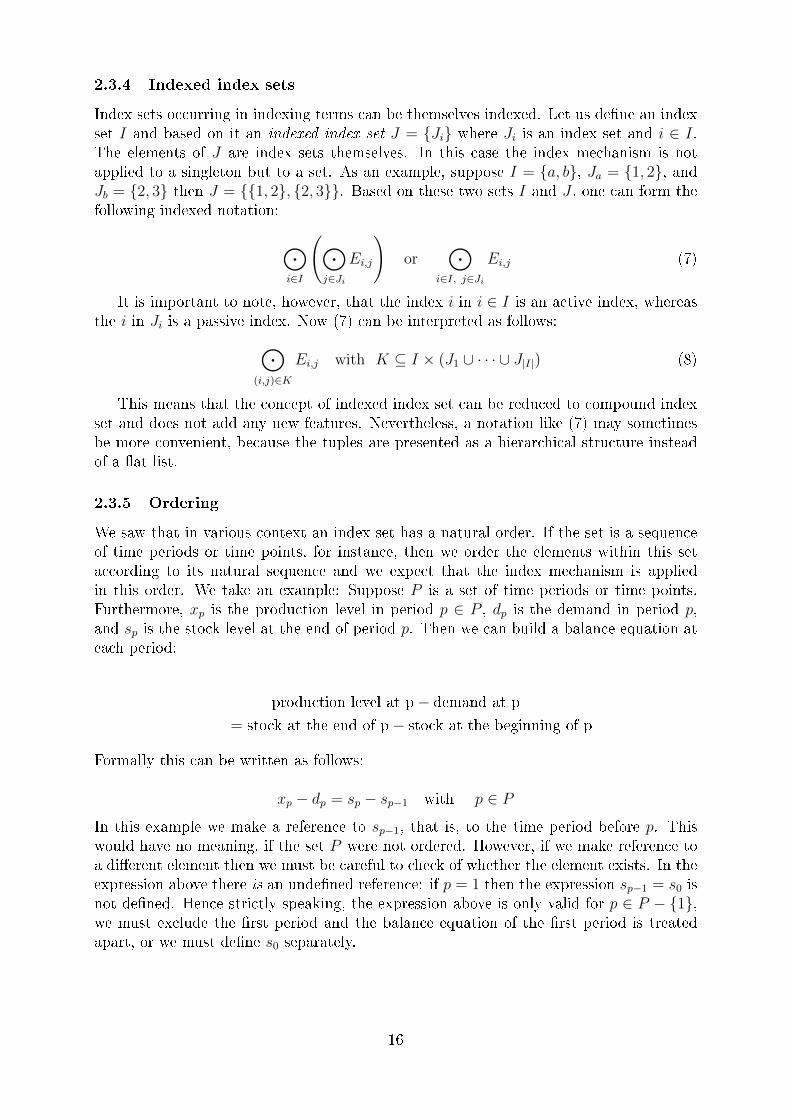
Index sets occurring in indexing terms can be themselves indexed. Let us de�ne an indexset I and based on it an indexed index set J = {Ji} where Ji is an index set and i ∈ I.The elements of J are index sets themselves. In this case the index mechanism is notapplied to a singleton but to a set. As an example, suppose I = {a, b}, Ja = {1, 2}, andJb = {2, 3} then J = {{1, 2}, {2, 3}}. Based on these two sets I and J , one can form thefollowing indexed notation:

⊙i∈I

(⊙j∈Ji

Ei,j

)or

⊙i∈I, j∈Ji

Ei,j (7)

It is important to note, however, that the index i in i ∈ I is an active index, whereasthe i in Ji is a passive index. Now (7) can be interpreted as follows:⊙

(i,j)∈K

Ei,j with K ⊆ I × (J1 ∪ · · · ∪ J|I|) (8)

This means that the concept of indexed index set can be reduced to compound indexset and does not add any new features. Nevertheless, a notation like (7) may sometimesbe more convenient, because the tuples are presented as a hierarchical structure insteadof a �at list.

2.3.5 Ordering

We saw that in various context an index set has a natural order. If the set is a sequenceof time periods or time points, for instance, then we order the elements within this setaccording to its natural sequence and we expect that the index mechanism is appliedin this order. We take an example: Suppose P is a set of time periods or time points.Furthermore, xp is the production level in period p ∈ P , dp is the demand in period p,and sp is the stock level at the end of period p. Then we can build a balance equation ateach period:

production level at p− demand at p

= stock at the end of p− stock at the beginning of p

Formally this can be written as follows:

xp − dp = sp − sp−1 with p ∈ P

In this example we make a reference to sp−1, that is, to the time period before p. Thiswould have no meaning, if the set P were not ordered. However, if we make reference toa di�erent element then we must be careful to check of whether the element exists. In theexpression above there is an unde�ned reference: if p = 1 then the expression sp−1 = s0 isnot de�ned. Hence strictly speaking, the expression above is only valid for p ∈ P − {1},we must exclude the �rst period and the balance equation of the �rst period is treatedapart, or we must de�ne s0 separately.

16

3 Index Notation in LPL

LPL is a computer language that implements basically the index mechanism described.In this section, this implementation is presented. For a general reference of the LPLlanguage see the Reference Manual (see [2]). LPL implements the indexed notation asclose as possible to the mathematical notation. But there are some di�erences. By meanof several examples, we explain the relationship.

In an LPL code, one needs to specify the index sets �rst. They are available throughoutthe whole model code. This is done by a declaration that begins with a keyword set. Itis followed by the name of the set and an assignment of the elements as follows:

set I := 1..10;set J := 1..100;parameter n;set K := 1..n;

This declaration de�nes the three sets I = {1 . . . 10}, J = {1 . . . 100} and a set K ={1 . . . n}. Note that n must be declared before K. It can or cannot have a value.

This set declarations can be used in expressions. The following expressions:

A =∑i∈I

1 , B =∑j∈J

j , C =∑

x∈J |10≤x≤20

x2

can be implemented directly as follows:

parameter A := sum{i in I} 1;parameter B := sum{j in J} j;parameter C := sum{x in J|x>=10 and x<=20} x^2;

The index operator∑

is the keyword sum. The indexing term i ∈ I is appended to theindex operator and bracketed with { and }. We also need to declare new parameters A, B,and C that hold the calculated value. The indexing condition is a proper Boolean expres-sion in the language. Hence 10 ≤ x ≤ 20 must be formulated as x>=10 and x<=20.Note that we use := as an assignment operator.

If we use tables such as vi, ai,j, and bi,j,k with i ∈ I, j ∈ J, k ∈ K, we must declarethem �rst in the code as follows:

parameter v{i in I};parameter a{i in I, j in J};parameter b{i in I, j in J, k in K};

Using these declaration we now can build other expressions like:

D =∑i∈I

vi , E = maxi∈I

(∑j∈J

ai,j

), Fk∈K =

∑i∈I, j∈J

bi,j,k

using the following syntax:

parameter D := sum{i in I} v[i];parameter E := max{i in I} (sum{j in J} a[i,j]);parameter F{k in K} := sum{i in I, j in J} b[i,j,k];

The passive indexes in the indexed expression are enclosed in the brackets [ and ]. Sothere is a clear syntactical distinction between the passive and the active indexes in thelanguage.

In LPL there exist a slightly shorter syntax that could also be used for an indexingterm. The examples above could be coded as follows:

17

set i := 1..10;set j := 1..100;parameter n;set k := 1..n;

parameter A := sum{i} 1;parameter B := sum{j} j;parameter C := sum{j|j>=10 and j<=20} j^2;

parameter v{i};parameter a{i,j};parameter b{i,j,k};

parameter D := sum{i} v[i];parameter E := max{i} (sum{j} a[i,j]);parameter F{k} := sum{i,j} b[i,j,k];

In this code, the active index has the same name as the corresponding index set. Hence,{i in I}, an indexing term, can just be written as {i}. This makes the expressionsmore readable and � in most context � much shorter. However, this can lead to di�cultiesas soon as the same index set is used more than once in an indexed expression as in thefollowing simple expression:

H =∑i,j∈I

ci,j

In such a case, LPL allows one to de�ne one or two alias names for the same index set.We then could code this as following:

set i, j := 1..10;parameter c{i,j};parameter H := sum{i,j} c[i,j];

Of course, one always can use the more �traditional� notation as follows:

set I := 1..10;parameter c{i in I, j in J}parameter H := sum{i in I,j in I} c[i,j];

The alias names � separated by commas � are just other names for the index set andcan be used as unique active indexes name in indexed notations. LPL allows at most twoaliases for each index sets. If we use more than two, then we always need to use the longersyntax as in the following example:

L =∑

i,j,k,p∈I

di,j,k,p

in which case we need to code this as:

set i, j,k := 1..10;parameter d{i,j,k,p in i};parameter L := sum{i,j,k,p in i} d[i,j,k,p];

The two versions of the LPL code can be downloaded or executed directly at: exercise0a2 and exercise0b 3

2http://lpl.unifr.ch/lpl/Solver.jsp?name=/exercise0a3http://lpl.unifr.ch/lpl/Solver.jsp?name=/exercise0b

18

Let us now code the Exercise 1 given in section 2.3.3 as an LPL model. First weimplement the declarations: The set of products and factories which are P = {1, 2, 3}and F = {1, 2, 3, 4} the cost table ci,j, the value table vp and the quantity table xp,i,j withi, j ∈ F and p ∈ P . In LPL these data tables can be implemented as follows:

set p := 1..3;set i, j := 1..4;parameter c{i,j|i<>j} := [. 1 5 2 , 2 . 4 2 , 1 2 . 3 , 1 3 1 .];parameter v{p} := [6 2 3];parameter x{p,i,j|i<>j} := [

. 48 37 45 36 . 43 46 44 36 . 33 36 39 34 . ,

. 46 35 39 32 . 47 35 45 49 . 39 47 46 30 . ,

. 32 32 40 30 . 41 30 45 43 . 45 44 41 34 . ];

In table c and x we use the indexing condition i<>j because there is no cost or quantityde�ned form a factory to itself. The data itself are listed in a lexico-graphical order. Theexpressions given in section 2.3.3 are then formulated as follows in LPL:

parameter T := sum{p,i,j} c[i,j]*x[p,i,j];parameter V := sum{p,i,j} v[p]*x[p,i,j];parameter C{p} := sum{i,j} c[i,j]*x[p,i,j];parameter W{i,j}:= sum{p} v[p]*x[p,i,j];parameter M{i} := max{p,j} x[p,i,j];parameter S{i} := max{p} (sum{j} x[p,i,j]);

The complete model can be executed at: exercise1a 4.

Exercise 1 (continued):Let us now add a requirement that the transportation can only take place between a smallsubset of all (i, j) links between the factories i, j ∈ F . Hence, we need to introduce aproperty K(i, j) which is true if the transportation can take place between factory i andfactory j. We de�ne it as:

Ki,j∈F ={(1, 2) (1, 4) (2, 3) (3, 2) (4, 3)

}The tuple list means that the transportation can only occur from factory 1 to 2, from 1to 4, from 2 to 3, from 3 to 2 and from 4 to 3. Only 5 transportation links are allowed.The corresponding expressions are then as follows:(1) The total transportation costs T is calculated as follows:

T =∑

p∈P, i,j∈F |K(i,j)

ci,j · xp,i,j = 1524

(2) The total value transported is as follows:

V =∑

p∈P, i,j∈F |K(i,j)

vp · xp,i,j = 2148

(3) The total transportation costs Cp for each product p ∈ P is:

Cp∈P =∑

i,j∈F |K(i,j)

ci,j · xp,i,j =

511537476

4http://lpl.unifr.ch/lpl/Solver.jsp?name=/exercise1a

19

(4) The value Wi,j transported between all factories (i, j) ∈ F × F is:

Wi,j∈F |K(i,j) =∑p∈P

vp · xp,i,j =

− 476 388 −− − 475 −− 443 − −− − 366 −

(5) The maximum quantity Mi transported from a factory i ∈ F is:

Mi∈F = maxp∈P, j∈F |K(i,j)

xp,i,j =(48 47 49 34

)(6) For each product p ∈ P the sum of the maximum quantity Si transported from afactory i ∈ F is:

Si∈F = maxp∈P

∑j∈F |K(i,j)

xp,i,j

=

85474934

It is straightforward to code this in LPL. First we declare the table of property Ki,j asfollowing:

set k{i,j} := [ 1 2 , 1 4 , 2 3 , 3 2 , 4 3 ];

The property K(i, j) is simply declared as a set. In fact, in LPL k{i,j} de�nes a tuplelist which is a subset of the Cartesian Product of (i, j) ∈ I × I. In LPL, we can code theexpressions as follows:

parameter T := sum{p,i,j|k[i,j]} c[i,j]*x[p,i,j];parameter V := sum{p,i,j|k[i,j]} v[p]*x[p,i,j];parameter C{p} := sum{i,j|k[i,j]} c[i,j]*x[p,i,j];parameter W{i,j|k[i,j]} := sum{p} v[p]*x[p,i,j];parameter M{i} := max{p,j|k[i,j]} x[p,i,j];parameter S{i} := max{p} (sum{j|k[i,j]} x[p,i,j]);

Since in LPL k{i,j} is itself a set, it can be used as an index set. Hence, the previouscode could be written also as:

parameter T := sum{p,k[i,j]} c[i,j]*x[p,i,j];parameter V := sum{p,k[i,j]} v[p]*x[p,i,j];parameter C{p} := sum{k[i,j]} c[i,j]*x[p,i,j];parameter W{k[i,j]} := sum{p} v[p]*x[p,i,j];parameter M{i} := max{p,j|k[i,j]} x[p,i,j];parameter S{i} := max{p} (sum{j|k[i,j]} x[p,i,j]);

The di�erence is in the �rst four expressions. We wrote {p,k[i,j]} instead of {p,i,j|k[i,j]}.These two indexing terms de�ne the same set. Computationally, however, there can bea huge di�erence. While the �rst indexing term {p,i,j|k[i,j]} has cardinality of| P×I×I | the second indexing term {p,k[i,j]} only has cardinality of | P×K(i, j) |.The two version of LPL code can be downloaded or executed directly at: exercise1b 5 andexercise1c 6.

5http://lpl.unifr.ch/lpl/Solver.jsp?name=/exercise1b6http://lpl.unifr.ch/lpl/Solver.jsp?name=/exercise1c

20

4 A Complete Problem: Exercise 2

In this second exercise we are going to explore the cost of a given production plan.Suppose we want to manufacture 7 di�erent products. We have 4 identical factorieswhere 5 di�erent machines are installed. 20 di�erent raw products are used to assem-ble a product. Hence, we have a set of products P = {A,B,C,D,E, F,G}, a setof factories F = {F1, F2, F3, F4}, a set of machines M = {M1,M2,M3,M4,M5},and a set of raw materials R = {1 . . . 20}. Additionally, various tables are given withp ∈ P, f ∈ F, m ∈ M, r ∈ R: A table qp,m de�nes which product can be manufacturedon which machine. The table Rr,p says how many units of raw materials r are used tomanufacture a unit of product p. The table Hp,m|q(p,m) says how many hours of machinem it takes to manufacture one unit of product p. The table Rcr gives the cost of a unitof raw materials, the table Mcm gives the cost of machine m per hour, and the table Sp

is the selling price of product p. Finally, the table Qf,p,m|q(p,m) is a given production plan.It says how many units products to manufacture on which machine and in which factory.(We do not discuss here whether this production plan is good or not.) We suppose thatall products can be sold, and that a machine can only process one product at the sametime. We do not consider any other costs. A concrete data set is given in the LPL codeand at the end of this paper (see exercise2 7).

We now wanted to calculate various amounts:

(1) The total selling value TS is:

TS =∑

f∈F, p∈P, m∈M |q(p,m)

Sp ·Qf,p,m = 383646

(2) The total cost of raw material RC is:

RC =∑

f∈F, p∈P, m∈M, r∈R|q(p,m)

Rr,p ·Rcr ·Qf,p,m = 305882

(3) The total machine costs MC is:

MC =∑

f∈F, p∈P, m∈M |qp,m

Hp,m ·Mcm ·Qf,p,m = 24882

(4) The total pro�t TS is:

TP = TS −RC −MC = 52882

(5) The total quantity TQp produced for each product p is:

TQp =∑

f∈F, m∈M |qp,m

Qf,p,m =(188 228 175 135 89 261 391

)(6a) How long (in hours) does the production take on each machine m ∈ M and in each

factory f ∈ F?

7http://lpl.unifr.ch/lpl/Solver.jsp?name=/exercise2

21

Tif∈F,m∈M =∑

p∈P |q(p,m)

Hp,m ·Qf,p,m =

515 312 542 290 330548 224 554 324 273416 392 309 154 246472 216 695 154 452

(6b) How long (in hours) does the production take maximally until the last product leaves

a factory f ∈ F?

TIf∈F = maxm∈M

∑p∈P |q(p,m)

Hp,m ·Qf,p,m

=(542 554 416 695

)(7a) How big is the loss (gain) of each product (Lop∈P )?

Lop∈P =∑f,m

Sp ·Qf,p,m −∑f,m

(∑r

Rr,p ·Rcr +Hp,m ·Mcm

)·Qf,p,m

={55792 33450 −6320 −19305 10769 −3046 −18458

}(7b) Which products generate a loss (set LOp∈P )?

LOp∈P =∑f,m

Sp ·Qf,p,m −∑f,m

(∑r

Rr,p ·Rcr +Hp,m ·Mcm

)·Qf,p,m < 0

={C D F G

}(8) Which machines in which factories work more than 500 hours (set MOf∈F, m∈M)?

MOf,m =∑p

Hp,m ·Qf,p,m > 500

={(F1,M1) (F1,M3) (F2,M1) (F2,M3) (F4,M3)

}(9) Which machine and in which factory works more than any other machine (setMAf∈F, m∈M)?

8

MAf,m =

f = argmaxf

(∑p

Hp,m ·Qf,p,m

)∧ m = argmax

m

(∑p

Hp,m ·Qf,p,m

)={(F4,M3)

}(10) Which machine and in which factory has the least work to do (in hours) (set

MIf∈F, m∈M)?

8The operators argmax and argmin are two other index operators returning the element for which theindexed expression has the largest and the smallest value.

22

MIf,m =

f = argminf

(∑p

Hp,m ·Qf,p,m

)∧ m = argmin

m

(∑p

Hp,m ·Qf,p,m

)={(F3,M4)

}It is straightforward to implement this examples in the language LPL. First we declarethe given index sets and the tables as follows (the concrete data for the parameter tablescan be found in the LPL model):

setp := [A B C D E F G]; r := [1..20];m := [M1 M2 M3 M4 M5]; f := [F1 F2 F3 F4];q{p,m};

parameterQ{f,q}; S{p}; R{r,p}; H{q}; Rc{r}; Mc{m};

Based on these given data, we can then calculate the various expressions as follows9:

parameterTS := sum{f,q[p,m]} Q*S;RC := sum{f,p,m,r} R*Rc * Q;MC := sum{f,p,m} H*Mc * Q;TP := TS - RC - MC;Ti{f,m}:= sum{p} H*Q;TI{f}:= max{m} sum{p} Mc*Q;Lo{p} := sum{f,m} S*Q - sum{f,m}(sum{r} R*Rc + H*Mc)* Q;

setLO{p} := sum{f,m} S*Q - sum{f,m}(sum{r} R*Rc + H*Mc)* Q < 0;MO{f,m}:= sum{p} H*Q > 300;MA{f,m}:= f=argmax{f}(sum{p} Mc*Q) and m=argmax{m}(sum{p} Mc*Q);MI{f,m}:= f=argmin{f}(sum{p} Mc*Q) and m=argmin{m}(sum{p} Mc*Q);

5 Data for Exercise 2

The data of Exercise 2 are as follows:

q 10 =

− − 1 − 11 − 1 − −1 − − 1 −− − − − 11 − − − −− 1 1 − −1 − 1 1 −

H =

− − 8 − 84 − 7 − −7 − − 2 −− − − − 35 − − − −− 8 2 − −3 − 2 2 −

S =

491391156120221257184

9In LPL, it is quite common to leave out the passive indexes: this is very practical and shortens the

expressions. However, this practice should only be used by advanced users.10 �1� in the matrix means that the combination is possible. For example qB,M1 = 1 means that product

B can be manufactured on machine M1.

23

R =

− − − − − − 1− − − − − − −− 8 7 6 − − −− 6 − − 5 − −7 8 − − − − 5− 4 − 6 − − −7 − − 3 4 − 45 − − 8 − 7 −− − − − − 8 2− − 3 − − − −− − − − − − 45 − 6 4 − 7 6− 2 5 − − − 8− − 4 − − − 5− − 5 3 − − −− 1 − − − − −− 5 − 1 − 6 6− − 5 4 8 6 −− 4 − − 3 − −4 − − 8 − 5 3

Rc =

56737735844842385656

Mc =

23524

Qf=F1 =

− − 15 − 2721 − 40 − −19 − − 16 −− − − − 3838 − − − −− 39 40 − −36 − 31 43 −

Qf=F2 =

− − 15 − 1811 − 48 − −41 − − 18 −− − − − 4317 − − − −− 28 32 − −44 − 17 48 −

Qf=F3 =

− − 10 − 2416 − 15 − −24 − − 20 −− − − − 1811 − − − −− 49 31 − −43 − 31 19 −

Qf=F4 =

− − 36 − 4334 − 43 − −23 − − 14 −− − − − 3623 − − − −− 27 15 − −20 − 38 21 −

6 An Optimizing Problem Version

In the previous Exercise 2, several tables have been given to specify a concrete productionplan. They are as follows:

1. Given 7 di�erent products (p ∈ P )

2. Manufactured in 4 identical factories (f ∈ F )

24

3. By means of 5 identical machines in each factory (m ∈M)

4. Using 20 di�erent raw products (r ∈ R)

5. A table qp,m de�ning which product p can be manufactured on which machine m

6. A table Rr,p saying how many units of raw materials r are used to manufacture aunit of product p

7. A table Hp,m|q(p,m) de�ning the hours of machine m that is taken to manufactureone unit of product p

8. A table Rcr giving the cost of a unit of raw materials r

9. A table Mcm specifying the cost of machine m per hour of work

10. A table Sp giving the selling price of product p

11. Finally, a table Qf,p,m|qp,m saying how many unit of products p are manufactured infactory f by means of machine m.

Especially, the last table Q is a given table that speci�es the production plan. It isa given arbitrary plan without asking the question whether this plan is optimal in anysense. Let us now ask the question whether this plan could be changed without changingthe manufactured quantity of each product, just by switching the production quantityfrom one machine to another.

6.1 Version 1: the easy problem

Let's take a concrete example: The present production plan say to manufacture 40 units ofthe second product (B) in factory F1 with machine M3, that is we have: QF1,B,M3 = 40.These 40 units could also have been manufactured by machine M1, such that QF1,B,M3

becomes 0 and QF1,B,M1 becomes 61. Doing this, implies that the total machine costsMC would now be reduced to:

MC =∑

f∈F, p∈P, m∈M |q(p,m)

Hp,m ·Mcr ·Qf,p,m = 23802

instead of 24882, which is a cost reduction of 1080 units. We could use probably otherreassignment of the production plan in order to reduce the cost even further. However, wewould like to do this not on an experimental level, but on a systematic way. Hence, thequestion is: How should the production plan be, in order to minimize the total machinecosts? (Note that the raw material costs do not change, supposing that the quantitiesof products manufactured do not change.) Expressed in another way: how should theproduction plan, that is the matrix Qf,p,m, be assigned in order to make the machinecosts as small as possible.

At this point, thing become interesting: From the mathematical point of view, wenow have a model in which some data are unknown, that is the matrix Qf,p,m becomesan unknown, because we want to know how this matrix has to be �lled to attain our goal(the minimizing of costs). Our model is as follows:

25

1. Let us introduce a new variable (that is the unknown matrix) to represent thenew production plan as follows: QQf,p,m|qp,m ≥ 0, where QQf,p,m is the (unknown)quantity of product p to be manufactured at factory f by the means of the machinem

2. We would like to minimize the total machine costs

3. We also would like to produce the same quantity of each product as in the previousplan

There three conditions could be translated into the following mathematical model. Thismodel has to be solved to �nd the minimizing cost production plan. The model is a sfollows:

min∑

f∈F, p∈P, m∈M |q(p,m)

Hp,m ·Mcr ·QQf,p,m

subject to ∑f∈F, m∈M |qp,m

QQf,p,m = TQp , forall p ∈ P

The formulation of this model in LPL is as following (see exercise2a 11 for a completecode):

....integer variable QQ{f,q};constraint CA{p}: sum{f,m} QQ = sum{f,m} Q;minimize obj1: sum{f,p,m} H*Mc * QQ;....

The new assigned (optimal, that is �cost minimal�) production plan QQ is as follows:

Qf=F1 =

− − − − 188228 − − − −− − − 175 −− − − − 13589 − − − −− − 261 − −391 − − − −

Qf=F2 = 0, Qf=F3 = 0, Qf=F4 = 0

And the total machine costs are:

MC =∑

f∈F, p∈P, m∈M |qp,m

Hp,m ·Mcr ·QQf,p,m = 16006

This is a substantial machine cost reduction of more than 35% compared to the initial(somewhat arbitrary) production plan of Exercise 2 (from 24882 units to 16006 units).

However, there is no need to use the mathematical models approach to �nd this trivialresult! We could have found it by a simple thought: �One should assign as much work aspossible to the cheapest machine!� For example, machine M4 only costs 4 to manufactureone unit of product C, while machine M1 costs 14, the only alternative to produce C.

11http://lpl.unifr.ch/lpl/Solver.jsp?name=/exercise2a

26

Furthermore it is not important in which factory the product is manufactured, since theyare all identical. Hence, the total quantity 175 of product C should be manufactured bythe means of machine M4. The idea is similar for the other products.

To �nd the cheapest unit cost for each product and the machine that generates this,we can use two indexed expressions as follows:

(1) Calculate the cheapest amount of machine cost to manufacture a particular productp (Table Cwp).

Cwp∈P = minm|qp,m

Hp,m ·Mcm

={32 8 4 12 10 10 6

}(2) What is the machine m that manufactures the cheapest product p (Table CWp,m) ?

CWp,m = (m = argminm1∈M |qp,m1Hp,m1 ·Mcm1

={(A,M5) (B,M1) (C,M4) (D,M5) (E,M1) (F,M3) (G,M1)

}Nevertheless, there is a problem with this solution. It might be the cost minimizing

production plan, however the occupation time of the 5 machine in factory F1 is now asfollows:

Tif∈F,m∈M =∑

p∈P |q(p,m)

Hp,m ·QQf,p,m =

2530 0 522 350 19090 0 0 0 00 0 0 0 00 0 0 0 0

Machine M1 in factory F1 is heavily occupied while all machines in the other factoriesare idle! (Well, we might evenly distribute the production between the four factories bydividing the quantities QQf,p,m by four. If the division results not in integers, then weshall round up two and round down two.) Nevertheless, some machines are idle and othersare heavily occupied.

6.2 Version 2: Limit Capacity

At this point the problem is getting interesting if we add capacity requirements. Supposethat all machines work 10 hour per days, 5 days a week and we would like to manufactureall products within 10 weeks. Is this possible? This problem is all but easy to solve.In fact, we might use the same model as before with the additional constraints that nomachine should work more than 500 hours and still we want to minimize costs.

This constraint can be formulated as follows:∑p∈P

Hp,q ·QQf,p,m ≤ 500 , forall m ∈M, f ∈ F

The formulation of this model in LPL is as following (see exercise2b 12 for a completecode):

12http://lpl.unifr.ch/lpl/Solver.jsp?name=/exercise2b

27

....integer variable QQ{f,q};constraint CA{p}: sum{f,m} QQ = sum{f,m} Q;

CB{m,f}: sum{p} H*QQ <= 500;minimize obj1: sum{f,p,m} H*Mc * QQ;....

The new assigned (optimal, that is �cost minimal�) production plan QQ is now as follows:

Qf=F1 =

− − − − 62124 − − − −− − − − −− − − − −− − − − −− − − − −1 − − − −

Qf=F2 =

− − − − 6289 − − − −− − − 175 −− − − − 1− − − − −− − 250 − −48 − − − −

Qf=F3 =

− − − − 121 − − − −− − − − −− − − − 1341 − − − −− − 11 − −163 − − − −

Qf=F4 =

− − − − 5214 − − − −− − − − −− − − − −88 − − − −− − − − −− − 179 − −

The following table give the occupation of each machine with this production plan:

Tif∈F,m∈M =∑

p∈P |q(p,m)

Hp,m ·QQf,p,m =

499 0 0 0 496500 0 500 350 499498 0 22 0 498496 0 358 0 416

We see that no machine exceeds the occupation time of 500 hours. All products will

be manufactured within 10 weeks.Still some machine are not at their capacity limit and some are still idle. Could we

reduce the overall production time and to what extend? The most simple way to do thisis to experiment with the maximal occupation time. Very quickly we �nd that we canreduce that time up to 330 hours, which means that the production can be terminatedwithin less than 7 weeks. The corresponding production plan now is as follows:

Qf=F1 =

− − 33 − 413 − − − −− − − − −− − − − −63 − − − −− 41 − − −1 − 32 55 −

Qf=F2 =

− − 41 − −80 − − − −− − − 9 −− − − − 1102 − − − −− 38 − − −− − 1 50 −

28

Qf=F3 =

− − − − 3880 − 10 − −− − − − −− − − − 62 − − − −− 41 99 − −− − 30 55 −

Qf=F4 =

− − − − 3454 − − − −− − 165 − −− − − − 1822 − − − −− 41 − − −− − 165 − −

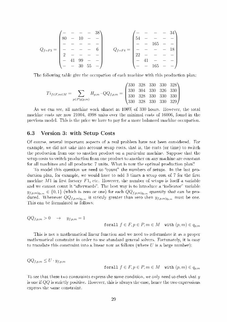
The following table give the occupation of each machine with this production plan:

Tif∈F,m∈M =∑

p∈P |q(p,m)

Hp,m ·QQf,p,m =

330 328 330 330 328330 304 330 326 330330 328 330 330 330330 328 330 330 329

As we can see, all machine work almost at 100% of 330 hours. However, the total

machine costs are now 21004, 4998 units over the minimal costs of 16006, found in theprevious model. This is the price we have to pay for a more balanced machine occupation.

6.3 Version 3: with Setup Costs

Of course, several important aspects of a real problem have not been considered. Forexample, we did not take into account setup costs, that is, the costs (or time) to switchthe production from one to another product on a particular machine. Suppose that thesetup costs to switch production from one product to another on any machine are constantfor all machines and all products: 7 units. What is now the optimal production plan?

To model this question we need to �count� the numbers of setups. In the last pro-duction plan, for example, we would have to add 3 times a setup cost of 7 for the �rstmachine M1 in �rst factory F1, etc. However, the number of setups is itself a variableand we cannot count it �afterwards�. The best way is to introduce a �indicator� variableyf,p,m|qp,m ∈ {0, 1} (which is zero or one) for each QQf,p,m|qp,m quantity that can be pro-duced. Whenever QQf,p,m|qp,m is strictly greater than zero then yf,p,m|qp,m must be one.This can be formulated as follows:

QQf,p,m > 0 → yf,p,m = 1

forall f ∈ F, p ∈ P,m ∈M with (p,m) ∈ qp,m

This is not a mathematical linear function and we need to reformulate it as a propermathematical constraint in order to use standard general solvers. Fortunately, it is easyto translate this constraint into a linear now as follows (where U is a large number):

QQf,p,m ≤ U · yf,p,mforall f ∈ F, p ∈ P,m ∈M with (p,m) ∈ qp,m

To see that these two constraints express the same condition, we only need to check that yis one if QQ is strictly positive. However, this is always the case, hence the two expressionsexpress the same constraint.

29

We now have to add all setup costs to the objective function. This function nowchanged to:

min∑

f∈F, p∈P, m∈M |q(p,m)

(Hp,m ·Mcr ·QQf,p,m + Setupp · yf,p,m)

The formulation of this model in LPL is as following (The value of U has been �xed to400 and the total machine occupation has slightly been increased to 337):

....integer variable QQ{f,q};binary variable y{f,q};constraint CA{p}: sum{f,m} QQ = sum{f,m} Q;

CB{m,f}: sum{p} H*QQ <= 337;CC{f,q}: QQ <= 400*y;

minimize obj1: sum{f,p,m} H*Mc * QQ + Setup*y;....

The solution can be look up by running the model exercise2c 13.

7 Conclusion

This paper gave a comprehensive overview of the indexed notation in mathematical mod-eling. The general notation is de�ned and several �extensions� have been explained. Itis fundamental to understand, read and write mathematical models. We then gave someexamples and how they are implemented in the modeling language LPL. Finally, a com-plete production model with several variants have been given in order to exercise themathematical notation on a concrete example.

References

[1] R.L. Graham, D.E. Knuth, and O. Patashnik. Concrete Mathematics. Addison�WesleyPubl. Comp, second edition, 1994.

[2] T. Hürlimann. Reference Manual for the LPL Modelling Language, most recent ver-sion. www.virtual-optima.com.

[3] T. Hürlimann. Mathematical Modelling and Optimization � An Essay for the Designof Computer-Based Modelling Tools. Kluwer Academic Publ., Dordrecht, 1999.

13http://lpl.unifr.ch/lpl/Solver.jsp?name=/exercise2c

30