index terms ijser engineering engineering in institute of technology, nirma university, inida,...

International Journal of Scientific & Engineering Research, Volume 7, Issue ƛ, JuÓà-2016 ISSN 2229-5518

IJSER © 2016

http://www.ijser.org

Modeling and Simulation of a Differential Drive Mobile Robot

Anirudh Topiwala

Abstract—Differential drive robots have wide application in the fields of defense, reconnaissance, in house hold applications like house cleansing robot

and many others. This paper intends to present a simple and a reliable method to circumvent the physical intricacies of the actual world, by developing a

realistic simulation system. A prototype model was first made to understand the logic of obstacle detection using ultrasonic sensors and Arduino Uno as

the microcontroller, but optimizing the robot physically by experimentation was very difficult. Therefore to solve this problem an identical simulation is

carried out in matlab for easy optimization. The Kinematic equations used to control the robot is presented.The output data of the kinematic model is

used to actuate the 3D model in virtual reality toolbox of matlab. The rotation of the robot about the central axis is also observed. The obstacles are de-

tected by the ultrasonic sensors mounted on the robot which enables the robot to navigate in an unknown environment.

Index Terms— Arduino, differential drive robot, kinematics, matlab, mobile robot, object avoidance, simulation, simulink.

—————————— ——————————

1 INTRODUCTION

Robotics today has become a part in our day to day life. We

can now develop highly maneuverable, functional and intelli-

gent robots for the high-end military applications to the more

mundane applications of the household. Locomotion system

for mobile robots can be broadly classified under legged and

wheeled systems. Legged robots are very useful under cir-

cumstances of extremely difficult terrain or when there are

high terrain discontinuities. The main advantage of this articu-

lated walking machines is that they can adapt their posture to

the uneven terrain making locomotion very easy. However,

articulated robots are difficult to control, have size restrictions

and are not as fast as compared to wheeled robots. [1]

Locomotion systems bases on wheels are relatively simple

as the number of articulations in a walking robot is far less

than that in a wheeled robot. Therefore, wheeled robot are far

faster, reliable simple and easy to control if it is required to

operate it on a rugged ground, roads, or any other relatively

level surface.[2]

Understanding how wheeled mobile robots (WMR) move

with reference to the command inputs is essential for naviga-

tion tasks like path planning, obstacle avoidance and guidance

systems.

2. Wheeled Mobile Robots

The wheeled mobile robots are classifies under five classes

corresponding to the pair of indices (m, s), where m is the mo-

bility degree and s is the steer ability. [3]

Class (3, 0) robots also called omnidirectional robots

have no steering wheels(s=0) that is they are only

equipped with Swedish or castor wheels. They have

complete mobility in a plane which means that they

can move in any direction without changing their ori-

entation. (m=3)

Class (2, 0) robots also have no steering wheel(s=0)

but at least one of the wheels is fixed with a common

axle, restricting the mobility of the plane to two-

dimensional motion in the plane.(m=2)

Class (2, 1) robots have at least one steering wheel

(s=1) and no fixed wheel, which means that all the

wheels can rotate independently. If the number of

steering wheels is more than two than they must be

coordinated and the mobility is restricted to a two

dimensional plane.(m=2)

Class (1, 1) robots have one or more fixed wheels on a

common axle and also one or more steering wheels

such that the centers of the steering wheels should not

coincide with the common axle of the fixed wheel and

the orientations must be coordinated.(s=1). The Mo-

bility of the robot depends upon the orientation of the

steering wheel and is restricted to one dimensional

plane.(m=1)

Class (1, 2) robots should at least have two steering

wheels(s=2) and no fixed wheel. The Mobility is de-

pendent on the orientation of the two steering wheels

and is restricted to one dimensional plane.(m=1)

————————————————

Anirudh Topiwala is currently pursuing bachlor’s degree program in mechanical engineering engineering in Institute of Technology, Nirma University, Inida, PH-+919712903712. E-mail: [email protected]

1410

IJSER

http://www.ijser.org/

International Journal of Scientific & Engineering Research Volume 7, Issue ƛȮɯ)ÜÓà-2016 ISSN 2229-5518

IJSER © 2016


In this paper I have developed a class (2, 0) type of differen-

tial drive robot.

3. The Prototype Model

3.1 The Mechanical aspects

The prototype model made here is of class (2, 0) [3] which

means that it has no steering wheel and the mobility is restrict-

ed to two dimensional plane. The chassis is made up of a rec-

tangular hard wood which has motor mountings mounted on

it.The two driving wheels used here are of plastic material and

has a rubber layer on them to increase the tractive force. To

balance the robot and preventing it from not falling over two

support castor wheels are added at the front and the back side.

If the material of the chassis is changed to aluminum than it

can have practical applications in industries as it can carry

heavy weights with high mobility and speed. The capability of

the robot to rotate about its own axis adds in to the advantages

of using it in industries.

(a)

(b)

Fig. 1. Front view of the prototype model showing different

components like ultrasonic sensors, bread board, Bluetooth

module, etc. (b) showing the remaining components which are

the Arduino uno board, 12V supply power, motor controller,

power bank to supply the Arduino board.

3.2 The Electronical aspects

An Arduino Uno board controls the robot. [4] The bot is

equipped with two high torque 800 rpm Robokits motors

which are bidirectional and operate at 12 volts. The motors are

mounted such that their axis of rotation is in one line. The two

ultrasonic sensors used here are of HC-SRO4 model that oper-

ate at 5 volts provided by the Arduino board. The Arduino

measures the distance by calculating the time required for the

ultrasonic waves emitted by the sensor to reflect back from

the obstacle. Using this data the Arduino determines whether

to take a left or right turn and change the direction of motor

accordingly with the help of motor controller. The motor con-

troller used here is RKI-1004(Robokits India). The motor con-

troller helps us connect a higher power source to the motors,

here it is 12 volts. Thus once the robot is able to detect obsta-

cles and move accordingly it just needs an input signal to start

after which it can act autonomously. A Bluetooth module con-

nected to the Arduino provides this input signal. The Blue-

tooth module used here is HC-06. . In case of any failures, this

Bluetooth module can also provide manual actuations to the

robot. Communication to the module can be established in

many ways, here we have developed an app in MIT appinven-

tor which uses a mobile phone’s Bluetooth to control the robot.

[5]

3.3 Need for simulation

While making the prototype robot we faced a lot of difficulties.

Some of them include the availability of certain components.

Also the sensors and the Arduino board used are very expen-

sive. Another important problem is the time required to exper-

iment different data values which can be easily done using

simulations. Optimizing the model experimentally can be a

painstaking task which can be easily and efficiently done using

different simulators. Graphs can be plotted between input and

output values to generate a comprehensive view of the collect-

ed data.

4. Differential Drive Robot

The mobile robot developed for the simulation is a class (2, 0)

type differential drive robot which is very similar to the proto-

type model developed. There are many design alternatives but

the two wheel drive robot is by far the most popular design.

The CAD software used to develop the model for simulation is

Solid Works 2014. The Differential drive robot consists of four

main parts which are the chassis, the wheels, the castor wheel

mounting and the castor wheel.

The chassis is cuboidal shaped and hollow at the center to ac-

commodate for the circuitry of the robot and also to reduce

weight of the robot. The chassis is symmetric about the central

planes which hepls the robot to rotate about the cental axis at

its own position.

Nomenclature

angular velocity of the robot R distance between ICC and the midpoint between the

wheels l distance between the wheels

rV linear velocity of the right wheel lV linear velocity of the left wheel

angle of the robot with X axis

1411

IJSER



IJSER © 2016


The different parts of the robot are connected to the chassis by

giving relations between the parts, which is called giving ma-

tes. The rotary parts are connected to the chassis by mainly

giving two mates the coincident mate and the cocentric ma-

te.The castor wheel is connected to the far end of the chassis

and is only used to give support to the robot. The two inde-

pendent driving wheels are connected to the front end of the

chassis

The robot also has eight ultrasonic sensor mountings on the

front side for the sensors. The mechanical integrity of the robot

is maintained by having a front bumper which protects the

robot from impacts or collisions.

Different parts of the model-robot have different material con-

siderations. Aluminium alloy is the preferred material of con-

stuction, because the parts are light in weight and are not very

expensive. The wheels have an aluminium rim and the tires

are made out of plastic which a rubber covering for traction.

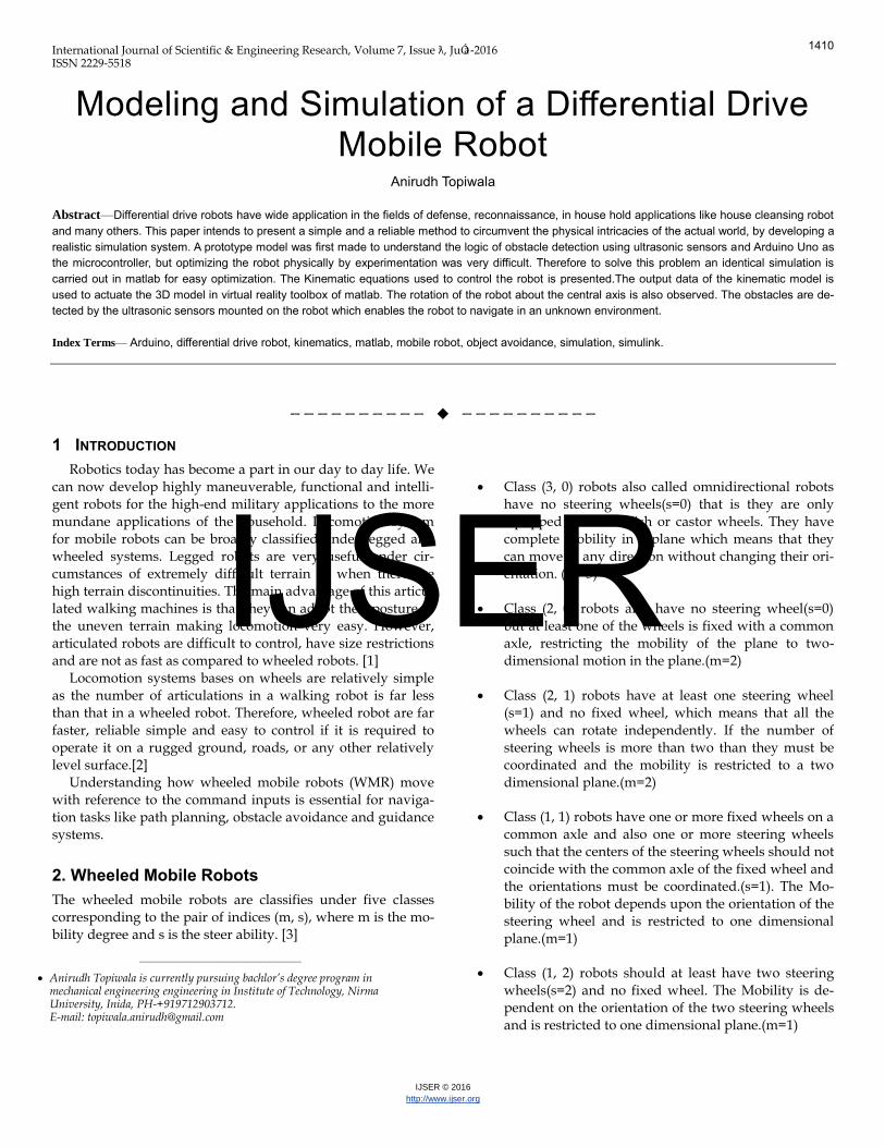
(a)

(b)

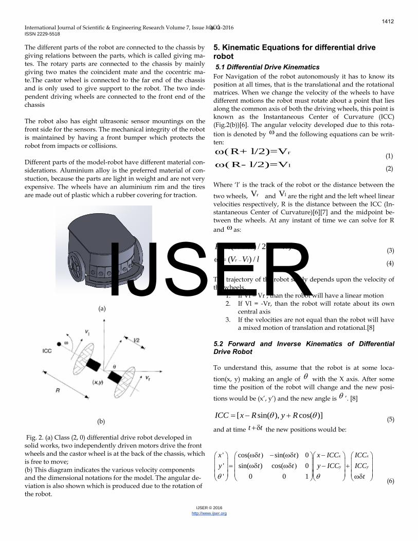
Fig. 2. (a) Class (2, 0) differential drive robot developed in solid works, two independently driven motors drive the front wheels and the castor wheel is at the back of the chassis, which is free to move; (b) This diagram indicates the various velocity components and the dimensional notations for the model. The angular de-viation is also shown which is produced due to the rotation of the robot.

5. Kinematic Equations for differential drive robot

5.1 Differential Drive Kinematics

For Navigation of the robot autonomously it has to know its position at all times, that is the translational and the rotational matrices. When we change the velocity of the wheels to have different motions the robot must rotate about a point that lies along the common axis of both the driving wheels, this point is known as the Instantaneous Center of Curvature (ICC) (Fig.2(b))[6]. The angular velocity developed due to this rota-

tion is denoted by and the following equations can be writ-ten:

rR+ l/2)=V (1)

lR- l/2)=V (2)

Where ‘l’ is the track of the robot or the distance between the

two wheels, r V and lV are the right and the left wheel linear velocities respectively, R is the distance between the ICC (In-stantaneous Center of Curvature)[6][7] and the midpoint be-tween the wheels. At any instant of time we can solve for R

and as:

( ) 2( )l r l rR l V V V V (3)

( ) /r lV V l (4)

The trajectory of the robot solely depends upon the velocity of the wheels,

1. If Vl = Vr , than the robot will have a linear motion 2. If Vl = -Vr, than the robot will rotate about its own

central axis 3. If the velocities are not equal than the robot will have

a mixed motion of translation and rotational.[8] 5.2 Forward and Inverse Kinematics of Differential Drive Robot To understand this, assume that the robot is at some loca-

tion(x, y) making an angle of with the X axis. After some time the position of the robot will change and the new posi-

tions would be (x’, y’) and the new angle is ’. [8]

[ sin( ), cos( )]ICC x R y R (5)

and at time t t the new positions would be:

' cos( sin( ) 0

' sin( ) cos( 0

' 0 0 1

x x

y y

x t t x ICC ICC

y t t y ICC ICC

t

(6)

1412

IJSER



IJSER © 2016


Using this equation we can find the position of the robot at any instant. To sum up the above equations we can describe the position of

the robot moving in a particular direction t at a given veloci-ty V (where V is the average of the left wheel and the right wheel velocity) by: [8] [9]

.sin .x tP x V d (7)

.cos .y tP y V d (8)

dt (9)

6. Simulation of Differential Drive Robot

In this section we will learn about the various simulations car-

ried out on the robot. The simulations are carried out in Sim-

ulink which is an extension of Matlab R2015A.

6.1 Basic Simulink Model

Once we are done with the modeling of the robot it is import-

ed into matlab using the Simulink Link add in in the CAD

software. The imported XML file is of second generation type.

The block diagram for the cad model is than generated using

the built in function H = smimport (“File Name.xml'). This

generates the block diagram wherein the relations between the

chassis and the different components can be easily seen. The

mates in the cad software for the robot are represented by rev-

olute blocks and can be altered so that we can change parame-

ters like internal mechanics, actuation, and sensing. [7] We can

give constant or varied velocity inputs to the robot through

this revolute block.

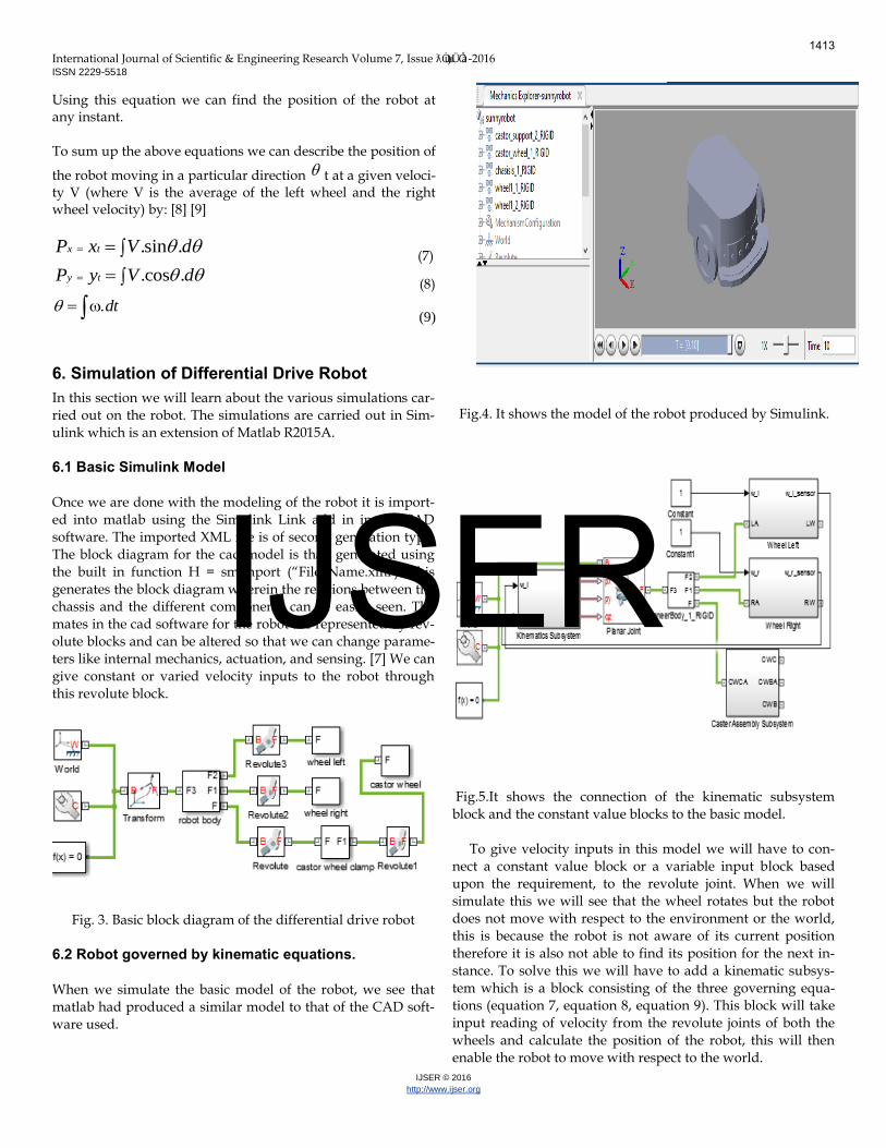
Fig. 3. Basic block diagram of the differential drive robot

6.2 Robot governed by kinematic equations.

When we simulate the basic model of the robot, we see that

matlab had produced a similar model to that of the CAD soft-

ware used.

Fig.4. It shows the model of the robot produced by Simulink.

Fig.5.It shows the connection of the kinematic subsystem

block and the constant value blocks to the basic model.

To give velocity inputs in this model we will have to con-

nect a constant value block or a variable input block based

upon the requirement, to the revolute joint. When we will

simulate this we will see that the wheel rotates but the robot

does not move with respect to the environment or the world,

this is because the robot is not aware of its current position

therefore it is also not able to find its position for the next in-

stance. To solve this we will have to add a kinematic subsys-

tem which is a block consisting of the three governing equa-

tions (equation 7, equation 8, equation 9). This block will take

input reading of velocity from the revolute joints of both the

wheels and calculate the position of the robot, this will then

enable the robot to move with respect to the world.

1413

IJSER



IJSER © 2016


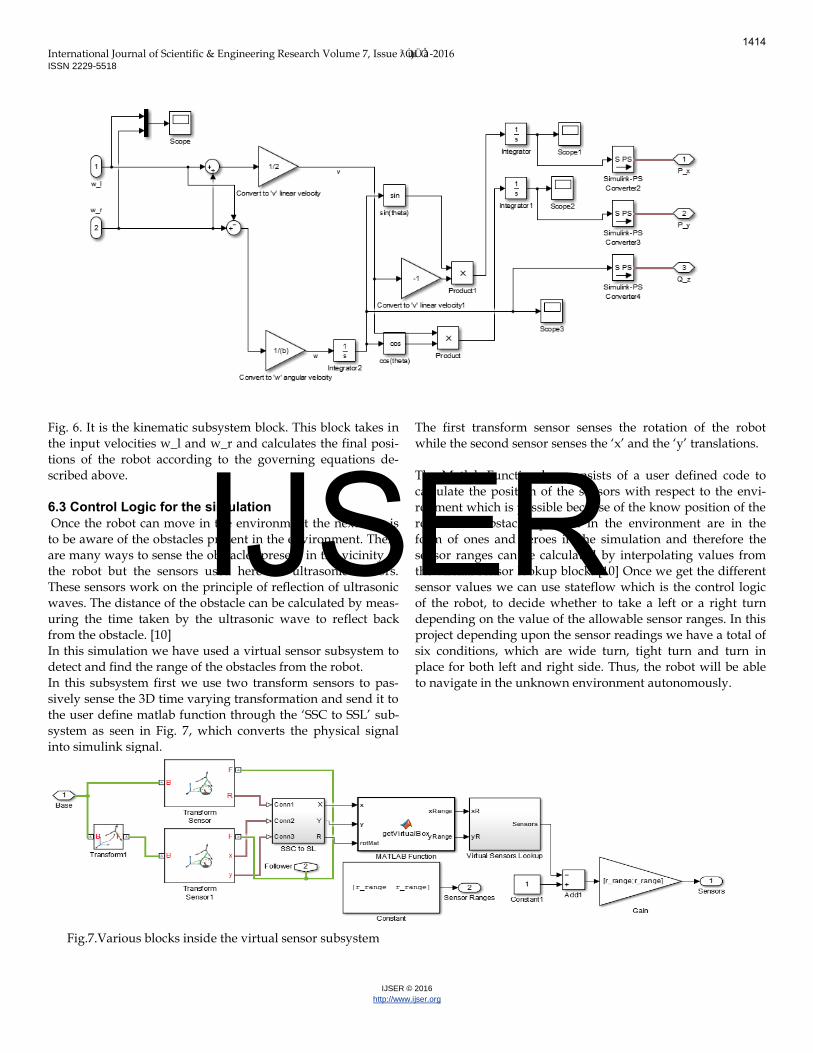
Fig. 6. It is the kinematic subsystem block. This block takes in

the input velocities w_l and w_r and calculates the final posi-

tions of the robot according to the governing equations de-

scribed above.

6.3 Control Logic for the simulation

Once the robot can move in the environment the next step is

to be aware of the obstacles present in the environment. There

are many ways to sense the obstacles present in the vicinity of

the robot but the sensors used here are ultrasonic sensors.

These sensors work on the principle of reflection of ultrasonic

waves. The distance of the obstacle can be calculated by meas-

uring the time taken by the ultrasonic wave to reflect back

from the obstacle. [10]

In this simulation we have used a virtual sensor subsystem to

detect and find the range of the obstacles from the robot.

In this subsystem first we use two transform sensors to pas-

sively sense the 3D time varying transformation and send it to

the user define matlab function through the ‘SSC to SSL’ sub-

system as seen in Fig. 7, which converts the physical signal

into simulink signal.

Fig.7.Various blocks inside the virtual sensor subsystem

The first transform sensor senses the rotation of the robot

while the second sensor senses the ‘x’ and the ‘y’ translations.

The Matlab Function box consists of a user defined code to

calculate the position of the sensors with respect to the envi-

ronment which is possible because of the know position of the

robot. The obstacles present in the environment are in the

form of ones and zeroes in the simulation and therefore the

sensor ranges can be calculated by interpolating values from

the virtual sensor lookup block. [10] Once we get the different

sensor values we can use stateflow which is the control logic

of the robot, to decide whether to take a left or a right turn

depending on the value of the allowable sensor ranges. In this

project depending upon the sensor readings we have a total of

six conditions, which are wide turn, tight turn and turn in

place for both left and right side. Thus, the robot will be able

to navigate in the unknown environment autonomously.

1414

IJSER



IJSER © 2016


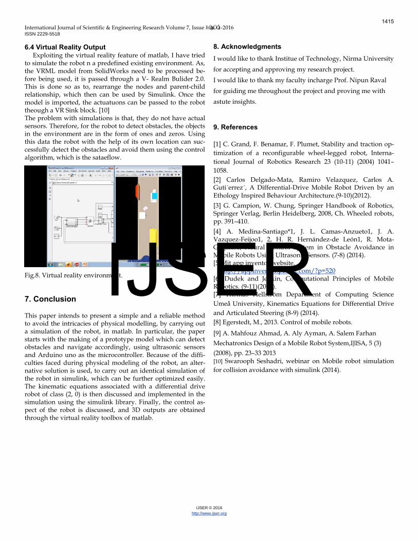
6.4 Virtual Reality Output Exploiting the virtual reality feature of matlab, I have tried

to simulate the robot n a predefined existing environment. As, the VRML model from SolidWorks need to be processed be-fore being used, it is passed through a V- Realm Bulider 2.0. This is done so as to, rearrange the nodes and parent-child relationship, which then can be used by Simulink. Once the model is imported, the actuatuons can be passed to the robot theough a VR Sink block. [10] The problem with simulations is that, they do not have actual sensors. Therefore, for the robot to detect obstacles, the objects in the environment are in the form of ones and zeros. Using this data the robot with the help of its own location can suc-cessfully detect the obstacles and avoid them using the control algorithm, which is the sataeflow.

Fig.8. Virtual reality environment.

7. Conclusion

This paper intends to present a simple and a reliable method to avoid the intricacies of physical modelling, by carrying out a simulation of the robot, in matlab. In particular, the paper starts with the making of a prototype model which can detect obstacles and navigate accordingly, using ultrasonic sensors and Arduino uno as the microcontroller. Because of the diffi-culties faced during physical modeling of the robot, an alter-native solution is used, to carry out an identical simulation of the robot in simulink, which can be further optimized easily. The kinematic equations associated with a differential drive robot of class (2, 0) is then discussed and implemented in the simulation using the simulink library. Finally, the control as-pect of the robot is discussed, and 3D outputs are obtained through the virtual reality toolbox of matlab.

8. Acknowledgments

I would like to thank Institue of Technology, Nirma University

for accepting and approving my research project.

I would like to thank my faculty incharge Prof. Nipun Raval

for guiding me throughout the project and proving me with

astute insights.

9. References

[1] C. Grand, F. Benamar, F. Plumet, Stability and traction op-

timization of a reconfigurable wheel-legged robot, Interna-

tional Journal of Robotics Research 23 (10-11) (2004) 1041–

1058.

[2] Carlos Delgado-Mata, Ramiro Velazquez, Carlos A. Guti´errez´, A Differential-Drive Mobile Robot Driven by an Ethology Inspired Behaviour Architecture.(9-10)(2012).

[3] G. Campion, W. Chung, Springer Handbook of Robotics, Springer Verlag, Berlin Heidelberg, 2008, Ch. Wheeled robots, pp. 391–410.

[4] A. Medina-Santiago*1, J. L. Camas-Anzueto1, J. A. Vazquez-Feijoo1, 2, H. R. Hernández-de León1, R. Mota-Grajales1, Neural Control System in Obstacle Avoidance in Mobile Robots Using Ultrasonic Sensors. (7-8) (2014). [5]Mit app inventor website. http://appinventor.pevest.com/?p=520 [6] Dudek and Jenkin, Computational Principles of Mobile Robotics. (9-11)(2013). [7] Thomas Hellström Department of Computing Science

Umeå University, Kinematics Equations for Differential Drive

and Articulated Steering (8-9) (2014).

[8] Egerstedt, M., 2013. Control of mobile robots.

[9] A. Mahfouz Ahmad, A. Aly Ayman, A. Salem Farhan

Mechatronics Design of a Mobile Robot System,IJISA, 5 (3)

(2008), pp. 23–33 2013 [10] Swarooph Seshadri, webinar on Mobile robot simulation

for collision avoidance with simulink (2014).

1415

IJSER


http://appinventor.pevest.com/?p=520

index terms ijser engineering engineering in institute of technology, nirma university, inida,...

Documents