Indexing by Latent Semantic Indexing by Latent Semantic AnalysisAnalysis

Scot Deerwester, Susan Dumais,George Furnas,Thomas Scot Deerwester, Susan Dumais,George Furnas,Thomas Landauer, and Richard HarshmanLandauer, and Richard Harshman

Presented by:Presented by:

Ashraf Ashraf KhalilKhalil

OutlineOutline

The ProblemSome HistoryLSAA Small ExampleEfficiencyOther applicationsSummary

The ProblemThe Problem

Given a collection of documents: retrieve documents that are relevant to a given query

Match terms in documents to terms in query

The ProblemThe Problem

The vector space method– term (rows) by document (columns) matrix,

based on occurrence– translate into vectors in a vector space

one vector for each document

– cosine to measure distance between vectors (documents)

small angle = large cosine = similar large angle = small cosine = dissimilar

The ProblemThe Problem

Two problems that arose using the vector space model:– synonymy: many ways to refer to the same

object, e.g. car and automobile leads to poor recall

– polysemy: most words have more than one distinct meaning, e.g. Jaguar

leads to poor precision

The GoalThe Goal

Latent Semantic Indexing was proposed to address these two problems with the vector space model

Some HistorySome History Latent Semantic Indexing was developed at

Bellcore (now Telcordia) in the late 1980s (1988). It was patented in 1989.

http://lsi.argreenhouse.com/lsi/LSI.html The first papers about LSI:

– Dumais, S. T., Furnas, G. W., Landauer, T. K. and Deerwester, S. (1988), "Using latent semantic analysis to improve information retrieval." In Proceedings of CHI'88: Conference on Human Factors in Computing, New York: ACM, 281-285.

– Deerwester, S., Dumais, S. T., Landauer, T. K., Furnas, G. W. and Harshman, R.A. (1990) "Indexing by latent semantic analysis." Journal of the Society for Information Science, 41(6), 391-407.

LSA: The ideaLSA: The idea

Idea (Deerwester et al):– “We would like a representation in which a set of terms, which by

itself is incomplete and unreliable evidence of the relevance of a given document, is replaced by some other set of entities which are more reliable indicants. We take advantage of the implicit higher-order (or latent) structure in the association of terms and documents to reveal such relationships.”

The assumption is that co-occurrence says something about semantics: words about the same things are likely to occur in the same contexts

If we have many words and contexts, small differences in co-occurrence probabilities can be compiled together to give information about semantics.

LSA: OverviewLSA: Overview Build a matrix with rows representing words and

columns representing context (a document or word string)

Apply SVD– unique mathematical decomposition of a matrix into the

product of three matrices: two with orthonormal columns-- (orthonormal)? one with singular values on the diagonal

– tool for dimension reduction– similarity measure based on co-occurrence– finds optimal projection into low-dimensional space

LSA MethodsLSA Methods

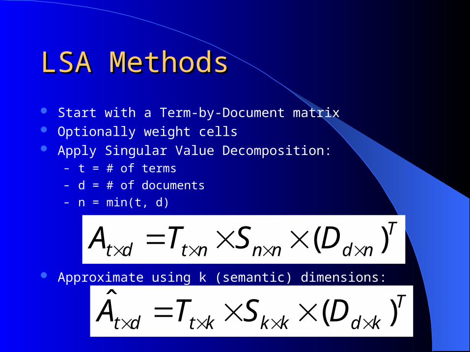
Start with a Term-by-Document matrix Optionally weight cells Apply Singular Value Decomposition:

– t = # of terms– d = # of documents– n = min(t, d)

Approximate using k (semantic) dimensions:

Tndnnntdt DSTA )(

Tkdkkktdt DSTA )(ˆ

LSA:LSA:

SVD– can be viewed as a method for rotating the axes

in n-dimensional space, so that the first axis runs along the direction of the largest variation among the documents

the second dimension runs along the direction with the second largest variation

and so on

– generalized least-squares method

LSALSA

Rank-reduced Singular Value Decomposition (SVD) performed on matrix– all but the k highest singular values are set to 0– produces k-dimensional approximation of the

original matrix– this is the “semantic space”

Compute similarities between entities in semantic space (usually with cosine)

A Small ExampleA Small Example

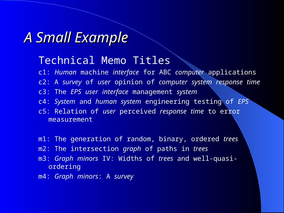
Technical Memo Titlesc1: Human machine interface for ABC computer applications

c2: A survey of user opinion of computer system response time

c3: The EPS user interface management system

c4: System and human system engineering testing of EPS

c5: Relation of user perceived response time to error measurement

m1: The generation of random, binary, ordered trees

m2: The intersection graph of paths in trees

m3: Graph minors IV: Widths of trees and well-quasi-ordering

m4: Graph minors: A survey

c1 c2 c3 c4 c5 m1 m2 m3 m4 human 1 0 0 1 0 0 0 0 0 interface 1 0 1 0 0 0 0 0 0 computer 1 1 0 0 0 0 0 0 0 user 0 1 1 0 1 0 0 0 0 system 0 1 1 2 0 0 0 0 0 response 0 1 0 0 1 0 0 0 0 time 0 1 0 0 1 0 0 0 0 EPS 0 0 1 1 0 0 0 0 0 survey 0 1 0 0 0 0 0 0 1 trees 0 0 0 0 0 1 1 1 0 graph 0 0 0 0 0 0 1 1 1 minors 0 0 0 0 0 0 0 1 1

A Small Example – 2A Small Example – 2

r (human.user) = -.38 r (human.minors) = -.29

A Small Example – 3A Small Example – 3

0.22 -0.11 0.29 -0.41 -0.11 -0.34 0.52 -0.06 -0.41 0.20 -0.07 0.14 -0.55 0.28 0.50 -0.07 -0.01 -0.11 0.24 0.04 -0.16 -0.59 -0.11 -0.25 -0.30 0.06 0.49 0.40 0.06 -0.34 0.10 0.33 0.38 0.00 0.00 0.01 0.64 -0.17 0.36 0.33 -0.16 -0.21 -0.17 0.03 0.27 0.27 0.11 -0.43 0.07 0.08 -0.17 0.28 -0.02 -0.05 0.27 0.11 -0.43 0.07 0.08 -0.17 0.28 -0.02 -0.05 0.30 -0.14 0.33 0.19 0.11 0.27 0.03 -0.02 -0.17 0.21 0.27 -0.18 -0.03 -0.54 0.08 -0.47 -0.04 -0.58 0.01 0.49 0.23 0.03 0.59 -0.39 -0.29 0.25 -0.23 0.04 0.62 0.22 0.00 -0.07 0.11 0.16 -0.68 0.23 0.03 0.45 0.14 -0.01 -0.30 0.28 0.34 0.68 0.18

T =

A Small Example – 4A Small Example – 4

S =3.34 2.54 2.35 1.64 1.50 1.31 0.85 0.56 0.36

A Small Example – 5A Small Example – 5

D = 0.20 0.61 0.46 0.54 0.28 0.00 0.01 0.02 0.08 -0.06 0.17 -0.13 -0.23 0.11 0.19 0.44 0.62 0.53 0.11 -0.50 0.21 0.57 -0.51 0.10 0.19 0.25 0.08 -0.95 -0.03 0.04 0.27 0.15 0.02 0.02 0.01 -0.03 0.05 -0.21 0.38 -0.21 0.33 0.39 0.35 0.15 -0.60 -0.08 -0.26 0.72 -0.37 0.03 -0.30 -0.21 0.00 0.36 0.18 -0.43 -0.24 0.26 0.67 -0.34 -0.15 0.25 0.04 -0.01 0.05 0.01 -0.02 -0.06 0.45 -0.76 0.45 -0.07 -0.06 0.24 0.02 -0.08 -0.26 -0.62 0.02 0.52 -0.45

A Small Example – 7A Small Example – 7

A Small Example – 7A Small Example – 7

r (human.user) = .94 r (human.minors) = -.83

c1 c2 c3 c4 c5 m1 m2 m3 m4

human 0.16 0.40 0.38 0.47 0.18 -0.05 -0.12 -0.16 -0.09

interface 0.14 0.37 0.33 0.40 0.16 -0.03 -0.07 -0.10 -0.04

computer 0.15 0.51 0.36 0.41 0.24 0.02 0.06 0.09 0.12

user 0.26 0.84 0.61 0.70 0.39 0.03 0.08 0.12 0.19

system 0.45 1.23 1.05 1.27 0.56 -0.07 -0.15 -0.21 -0.05

response 0.16 0.58 0.38 0.42 0.28 0.06 0.13 0.19 0.22

time 0.16 0.58 0.38 0.42 0.28 0.06 0.13 0.19 0.22

EPS 0.22 0.55 0.51 0.63 0.24 -0.07 -0.14 -0.20 -0.11

survey 0.10 0.53 0.23 0.21 0.27 0.14 0.31 0.44 0.42

trees -0.06 0.23 -0.14 -0.27 0.14 0.24 0.55 0.77 0.66

graph -0.06 0.34 -0.15 -0.30 0.20 0.31 0.69 0.98 0.85

minors -0.04 0.25 -0.10 -0.21 0.15 0.22 0.50 0.71 0.62

c1 c2 c3 c4 c5 m1 m2 m3 m4 human 1 0 0 1 0 0 0 0 0 interface 1 0 1 0 0 0 0 0 0 computer 1 1 0 0 0 0 0 0 0 user 0 1 1 0 1 0 0 0 0 system 0 1 1 2 0 0 0 0 0 response 0 1 0 0 1 0 0 0 0 time 0 1 0 0 1 0 0 0 0 EPS 0 0 1 1 0 0 0 0 0 survey 0 1 0 0 0 0 0 0 1 trees 0 0 0 0 0 1 1 1 0 graph 0 0 0 0 0 0 1 1 1 minors 0 0 0 0 0 0 0 1 1

A Small Example – 2 againA Small Example – 2 again

r (human.user) = -.38 r (human.minors) = -.29

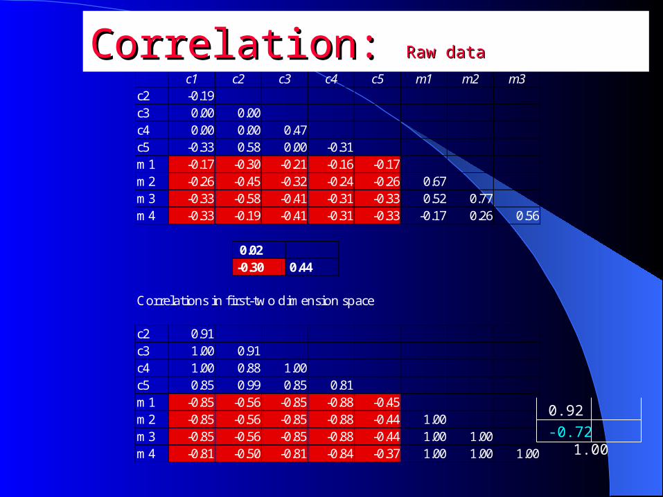
LSA Titles example: Correlations between titles in raw data

c1 c2 c3 c4 c5 m1 m2 m3 c2 -0.19 c3 0.00 0.00 c4 0.00 0.00 0.47 c5 -0.33 0.58 0.00 -0.31 m1 -0.17 -0.30 -0.21 -0.16 -0.17 m2 -0.26 -0.45 -0.32 -0.24 -0.26 0.67 m3 -0.33 -0.58 -0.41 -0.31 -0.33 0.52 0.77 m4 -0.33 -0.19 -0.41 -0.31 -0.33 -0.17 0.26 0.56

0.02 -0.30 0.44

Correlations in first-two dimension space c2 0.91 c3 1.00 0.91 c4 1.00 0.88 1.00 c5 0.85 0.99 0.85 0.81 m1 -0.85 -0.56 -0.85 -0.88 -0.45 m2 -0.85 -0.56 -0.85 -0.88 -0.44 1.00 m3 -0.85 -0.56 -0.85 -0.88 -0.44 1.00 1.00 m4 -0.81 -0.50 -0.81 -0.84 -0.37 1.00 1.00 1.00

Correlation: Correlation: Raw dataRaw data

0.92

-0.72 1.00

Some Issues with LSISome Issues with LSI

SVD Algorithm complexity O(n^2k^3) n = number of terms + documents k = number of dimensions in semantic space

(typically small ~50 to 350)

Although lot of empirical evidence no concrete proof of why LSI works

Semantic DimensionSemantic Dimension

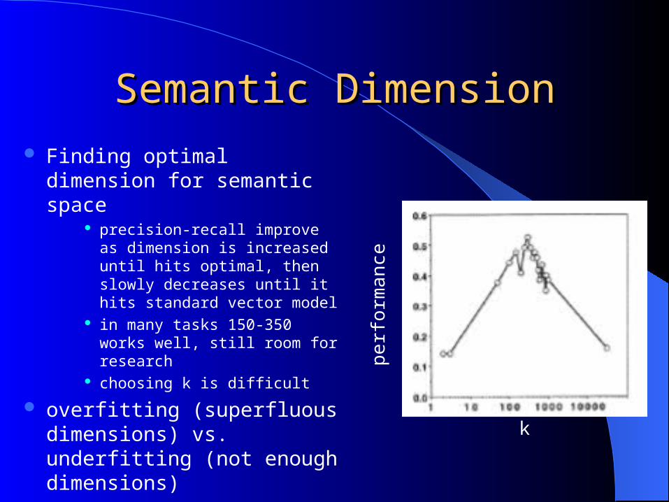
Finding optimal dimension for semantic space

precision-recall improve as dimension is increased until hits optimal, then slowly decreases until it hits standard vector model

in many tasks 150-350 works well, still room for research

choosing k is difficult

overfitting (superfluous dimensions) vs. underfitting (not enough dimensions) k

perf

orm

ance

Other ApplicationsOther Applications

Has proved to be a valuable tool in many areas as well as IR– summarization– cross-language IR– topics segmentation– text classification– question answering– LSA can pass the TOEFL

LSA can Pass the TOEFL LSA can Pass the TOEFL

Task:– Multiple-choice test for synonym– Given one word, find best match out of 4 alternatives

Training:– Corpus of 30,473 articles from Grolier’s Academic– Used first ~150 words from each article => 60,768 unique– words that occur at least twice– 300 singular vectors

Result– LSI gets 52.5% correct (corrected for guessing)– Non-LSI similarity gets 15.8% (other paper 29.5%) correct– Average (foreign) human test taker gets 52.7%

Landauer, T. K. and Dumais, S. T. (1997) A solution to Plato's problem: the Latent Semantic Analysis theory of acquisition, induction and representation of knowledge. Psychological Review, 104(2) 211-240.

LSA can mark essaysLSA can mark essays

LSA judgments of the quality of sentences correlate at r = 0.81 with expert ratings

LSA can judge how good an essay (on a well-defined set topic) is by computing the average distance between the essay to be marked and a set of model essays– The correlation are equal to between-human

correlations “If you wrote a good essay and scrambled the words you

would get a good grade," Landauer said. "But try to get the good words without writing a good essay!”

Good ReferencesGood ReferencesThe group at the University of Colorado at

Boulder has a web site where you can try out LSA and download papers– http://lsa.colorado.edu/

Papers are also available at:– http://lsi.research.telcordia.com/lsi/LSI.html