individual and market demand k copyright © 2013 worth publishers, all rights reserved ...
TRANSCRIPT

Individual and Market Demand k
Copyright © 2013 Worth Publishers, All Rights Reserved Microeconomics Goolsbee/Levitt/ Syverson 1/e
5Chapter outline5.1 How Income Changes Affect an Individual’s Consumption Choices5.2 How Price Changes Affect Consumption Choices5.3 Decomposing ConsumerResponses to Price Changes into
Income and Substitution Effects5.4 The Impact of Changes in Another Good’s Price 5.5 Combining Individual Demand Curves to Obtain the Market Demand Curve5.6 Conclusion
5-1

Introduction
Copyright © 2013 Worth Publishers, All Rights Reserved Microeconomics Goolsbee/Levitt/ Syverson 1/e 5-2
5With the consumer choice framework in place, we now link consumer decisions with individual and market demand
These links help determine
•Why shifts in tastes affect prices
•What benefits producers offer consumers
•How income and wealth affect purchase patterns
•What determines how consumers respond to price changes

5.1
Copyright © 2013 Worth Publishers, All Rights Reserved Microeconomics Goolsbee/Levitt/ Syverson 1/e 5-3
The income effect is the change in optimal consumption choices associated with a change in income (or purchasing power), holding relative prices constant
Is higher income associated with higher consumption of goods?
It depends!
For normal goods, higher income is associated with rising consumption•For instance, consider Fancy Meals and Vacations, both of which are considered normal goods
5How Income Changes Affect an Individual’s Consumption Choices

5.1
Copyright © 2013 Worth Publishers, All Rights Reserved Microeconomics Goolsbee/Levitt/ Syverson 1/e 5-4
5Figure 5.1 A Consumer's Response to an Increase in
Income When Both Goods Are Normal
How Income Changes Affect an Individual’s Consumption Choices
Vacations Incomerises
BAQv U2U1BC1 BC2Fancy mealsQm

5.1
Copyright © 2013 Worth Publishers, All Rights Reserved Microeconomics Goolsbee/Levitt/ Syverson 1/e 5-5
The income effect is the change in optimal consumption choices associated with a change in income (or purchasing power), holding relative prices constant
Is higher income associated with higher consumption of goods?
It depends!
For normal goods, higher income is associated with rising consumption
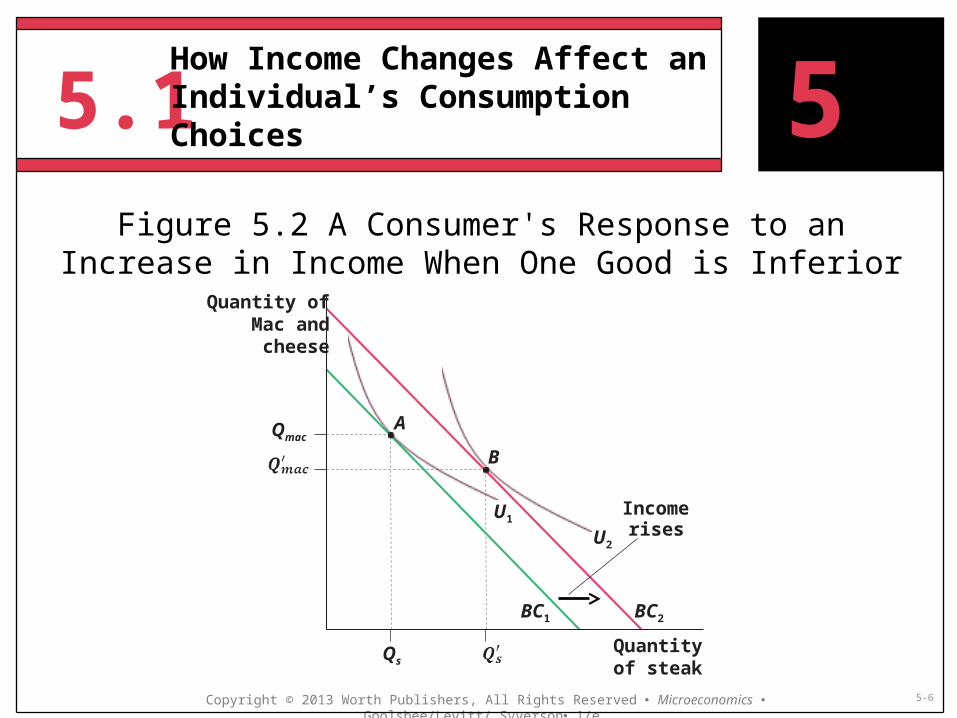
Alternatively, for inferior goods, higher income is associated with falling consumption•Consider boxed macaroni and cheese (inferior good) vs. steak (a normal good)
5How Income Changes Affect an Individual’s Consumption Choices
5.1
Copyright © 2013 Worth Publishers, All Rights Reserved Microeconomics Goolsbee/Levitt/ Syverson 1/e 5-6
5Figure 5.2 A Consumer's Response to an Increase in
Income When One Good is Inferior
How Income Changes Affect an Individual’s Consumption Choices
Quantity ofMac andcheeseAQmac B
IncomeU1 risesU2
BC1 BC2Quantityof steakQs

5.1
Copyright © 2013 Worth Publishers, All Rights Reserved Microeconomics Goolsbee/Levitt/ Syverson 1/e 5-7
Income Elasticities and Types of Goods
Chapter 2 introduced the concept of elasticity•Income elasticity describes the response of demand to changing income•Specifically, the percentage change in quantity consumed associated with a percentage change in income
Mathematically,
where I is income and Q is the quantity of a good demanded
The income effect is given by
5How Income Changes Affect an Individual’s Consumption Choices
Q
I
I
Q
II
I
QEDI
/
/
%
%
I
Q
5.1
Copyright © 2013 Worth Publishers, All Rights Reserved Microeconomics Goolsbee/Levitt/ Syverson 1/e 5-8
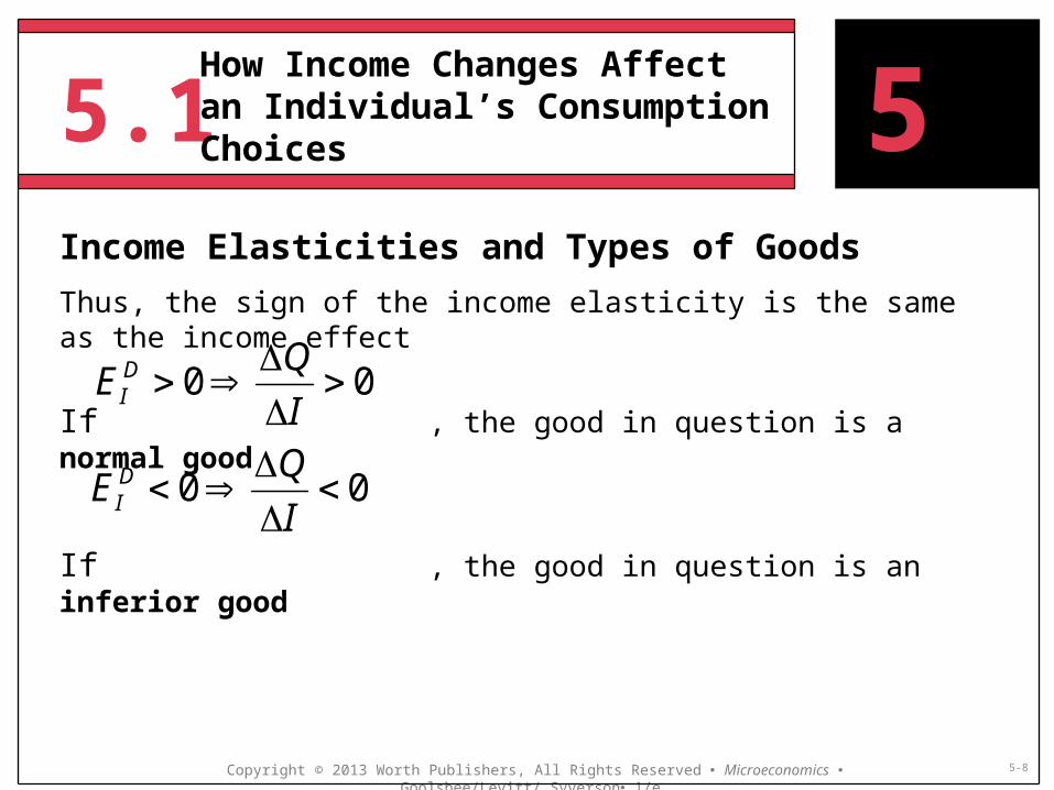
Income Elasticities and Types of Goods
Thus, the sign of the income elasticity is the same as the income effect
If , the good in question is a normal good
If , the good in question is an inferior good
5How Income Changes Affect an Individual’s Consumption Choices
00
I
QEDI
00
I
QEDI

Application
Copyright © 2013 Worth Publishers, All Rights Reserved Microeconomics Goolsbee/Levitt/ Syverson 1/e 5-9
Is the Environment a Normal Good?
While usually not priced in the market, consumers have preferences for environmental quality just like any other good•Most economists believe the environment is a normal good•Poorer countries are often characterized by environmentally damaging industrial processes; perhaps citizens are choosing improved income over environmental quality•As income-per-capita improves, pollution should fall•This hypothesis is known as the “Environmental Kuznets Curve” (EKC)
Vollebergh, et al. (2009) find evidence for the EKC for sulfur dioxide emissions in a panel of OECD countries
They find no similar evidence for carbon dioxide
Images: FreeDigitalPhotos.net
5
Citation: Vollebergh, H. R. J., Melenberg, B., and Dijkgraff, E. 2009. “Identifying reduced form relations with panel data: The case of pollution and income.” Journal of Environmental Economics and Management 58: 27-42.
Application
Copyright © 2013 Worth Publishers, All Rights Reserved Microeconomics Goolsbee/Levitt/ Syverson 1/e 5-10
5
Citation: Vollebergh, H. R. J., Melenberg, B., and Dijkgraff, E. 2009. “Identifying reduced form relations with panel data: The case of pollution and income.” Journal of Environmental Economics and Management 58: 27-42.
Income per capita
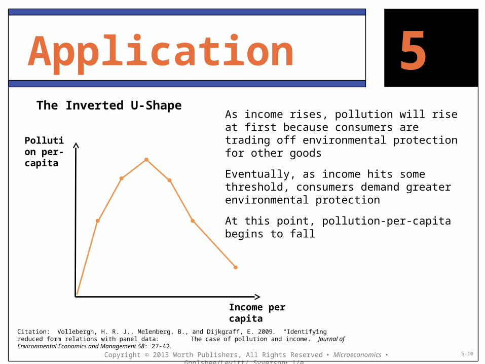
The Inverted U-Shape
Pollution per-capita
As income rises, pollution will rise at first because consumers are trading off environmental protection for other goods
Eventually, as income hits some threshold, consumers demand greater environmental protection
At this point, pollution-per-capita begins to fall

Application
Copyright © 2013 Worth Publishers, All Rights Reserved Microeconomics Goolsbee/Levitt/ Syverson 1/e 5-11
Caveats:•Because markets for environmental goods and services are often lacking or non-existent, they are often under-supplied •Without strong property rights or an effective central authority, the EKC hypothesis will likely fail•Additionally, as income grows, production processes generally become more efficient on their own, and economies transition to less polluting service sectors•Many economists dispute the presence of a demand-driven inverted U-shape for most pollutants
Images: FreeDigitalPhotos.net
5
Citation: Vollebergh, H. R. J., Melenberg, B., and Dijkgraff, E. 2009. “Identifying reduced form relations with panel data: The case of pollution and income.” Journal of Environmental Economics and Management 58: 27-42.
5.1
Copyright © 2013 Worth Publishers, All Rights Reserved Microeconomics Goolsbee/Levitt/ Syverson 1/e 5-12
5How Income Changes Affect an Individual’s Consumption Choices

Copyright © 2013 Worth Publishers, All Rights Reserved Microeconomics Goolsbee/Levitt/ Syverson 1/e 5-13
Figure it outEating out vs. paperback books
Copyright © 2013 Worth Publishers, All Rights Reserved Microeconomics Goolsbee/Levitt/ Syverson 1/e 5-14
Figure it outEating out vs. paperback books
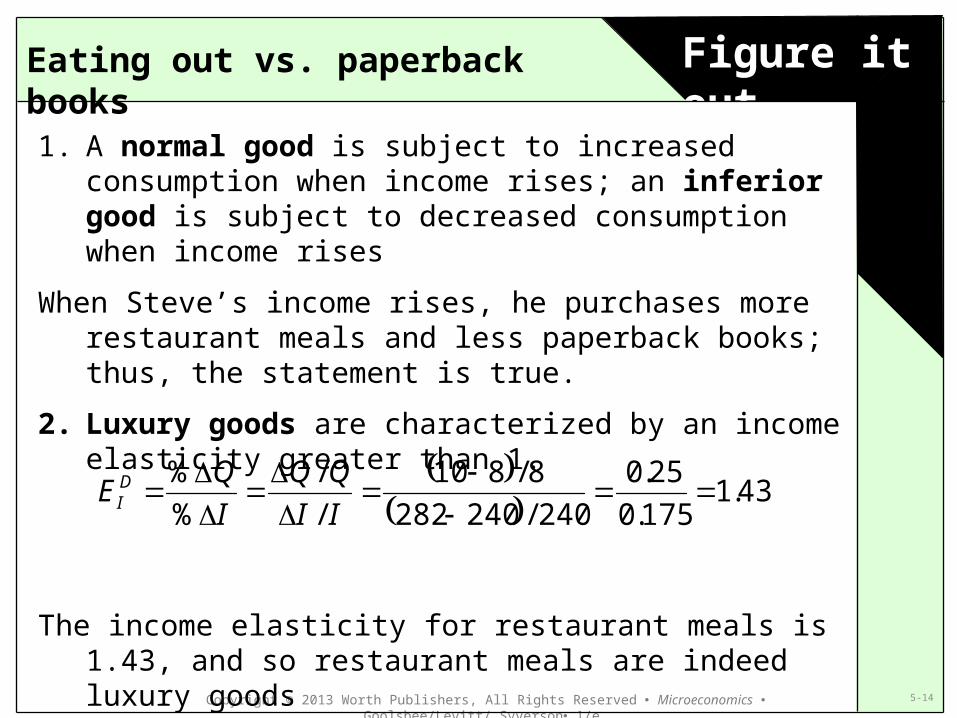
1. A normal good is subject to increased consumption when income rises; an inferior good is subject to decreased consumption when income rises
When Steve’s income rises, he purchases more restaurant meals and less paperback books; thus, the statement is true.
2. Luxury goods are characterized by an income elasticity greater than 1.
The income elasticity for restaurant meals is 1.43, and so restaurant meals are indeed luxury goods
43.1
175.0
25.0
240/240282
8/810
/
/
%
%
II
I
QEDI
Copyright © 2013 Worth Publishers, All Rights Reserved Microeconomics Goolsbee/Levitt/ Syverson 1/e 5-15
Figure it outEating out vs. paperback books
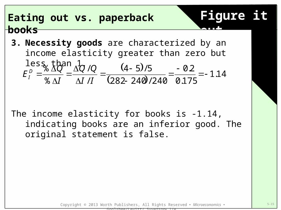
3. Necessity goods are characterized by an income elasticity greater than zero but less than 1.
The income elasticity for books is -1.14, indicating books are an inferior good. The original statement is false.
14.1
175.0
2.0
240/240282
5/54
/
/
%
%
II
I
QEDI
5.1
Copyright © 2013 Worth Publishers, All Rights Reserved Microeconomics Goolsbee/Levitt/ Syverson 1/e 5-16
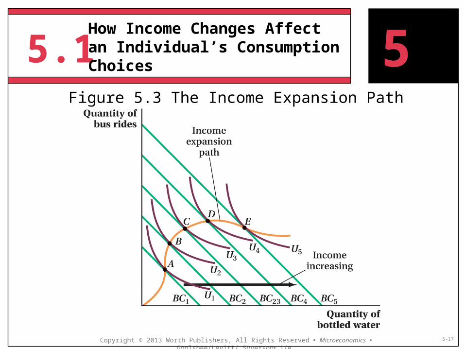
Tracing the optimal bundle of goods chosen as income increases results in the income expansion path•Helps determine whether a good is normal or inferior, but only two goods represented•Can’t directly observe income levels on the curve (both axes represent quantities of goods)
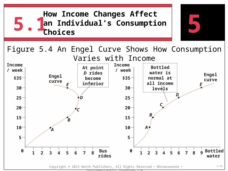
A more common way to describe the consumption-income relationship is with an Engel curve•Shows the relationship between quantity consumed of one good and consumer income
5How Income Changes Affect an Individual’s Consumption Choices
5.1
Copyright © 2013 Worth Publishers, All Rights Reserved Microeconomics Goolsbee/Levitt/ Syverson 1/e 5-17
Figure 5.3 The Income Expansion Path
5How Income Changes Affect an Individual’s Consumption Choices
5.1
Copyright © 2013 Worth Publishers, All Rights Reserved Microeconomics Goolsbee/Levitt/ Syverson 1/e 5-18
5Figure 5.4 An Engel Curve Shows How Consumption
Varies with Income
How Income Changes Affect an Individual’s Consumption Choices
Income/ week Engel$35 curve E3025 D20 C15 B10 A5
0 Bus1 2 3 4 5 6 7 8 rides
Income / week Engel$35 curveE30 D25 C20 B15 A1050 1 2 3 4 5 6 7 8 Bottledwater9
At point D rides become inferiorBottled water is normal at all income levels

Application
Copyright © 2013 Worth Publishers, All Rights Reserved Microeconomics Goolsbee/Levitt/ Syverson 1/e 5-19
5
Citation: Vollebergh, H. R. J., Melenberg, B., and Dijkgraff, E. 2009. “Identifying reduced form relations with panel data: The case of pollution and income.” Journal of Environmental Economics and Management 58: 27-42.
Income per capita
The EKC Hypothesis revisited
Pollution per-capita
Returning to the previous example, we can uncover how the U-shape is equivalent to an Engle curve by switching the axes
While environmental quality is a normal good, pollution is an inferior good, as the shape of this curve suggests
5.2
Copyright © 2013 Worth Publishers, All Rights Reserved Microeconomics Goolsbee/Levitt/ Syverson 1/e 5-20
Just as income affects consumer choices, changes in relative prices—holding income constant—also affects these choices
Deriving a Demand Curve•Demand curves define a relationship between quantity demanded and price•To derive a demand curve, we must understand how a consumer responds to a change in price•By changing one price on an indifference curve – budget constraint map, we can observe changes to consumer choices and then build the demand curve for an individual•The observed price represents the maximum willingness to pay for the last unit consumed
5How Price Changes Affect Consumption Choices

5.2
Copyright © 2013 Worth Publishers, All Rights Reserved Microeconomics Goolsbee/Levitt/ Syverson 1/e 5-21
5Figure 5.7 Building an Individual's Demand Curve
How Price Changes Affect Consumption Choices
Mountain Dew PG = 4 PG = 1(2 liter bottles) Income = $20PG = $1PMD = $2PG = 210432 U1U3 U20 3 5 8 14 20Quantity of grape juice(1 liter bottles)
Price ofgrape juice($/bottle)Carolyn’s$4 demand for2 grape juice10 3 8 14Quantity of grape juice(1 liter bottles)
10

5.2
Copyright © 2013 Worth Publishers, All Rights Reserved Microeconomics Goolsbee/Levitt/ Syverson 1/e 5-22
Shifts in the Demand Curve
When consumer preferences, income, or the prices of other goods change, the demand curve will shift
Consider the example of Mountain Dew and grape juice from the previous figure•Imagine the consumer prefers the taste of Mountain Dew, but had previously limited consumption due to worries about high fructose corn syrup•After hearing advertisements from the Corn Refiners Association claiming corn syrup is identical to cane sugar, her fears are reduced
What might happen to the demand for grape juice?
5How Price Changes Affect Consumption Choices
5.2
Copyright © 2013 Worth Publishers, All Rights Reserved Microeconomics Goolsbee/Levitt/ Syverson 1/e 5-23
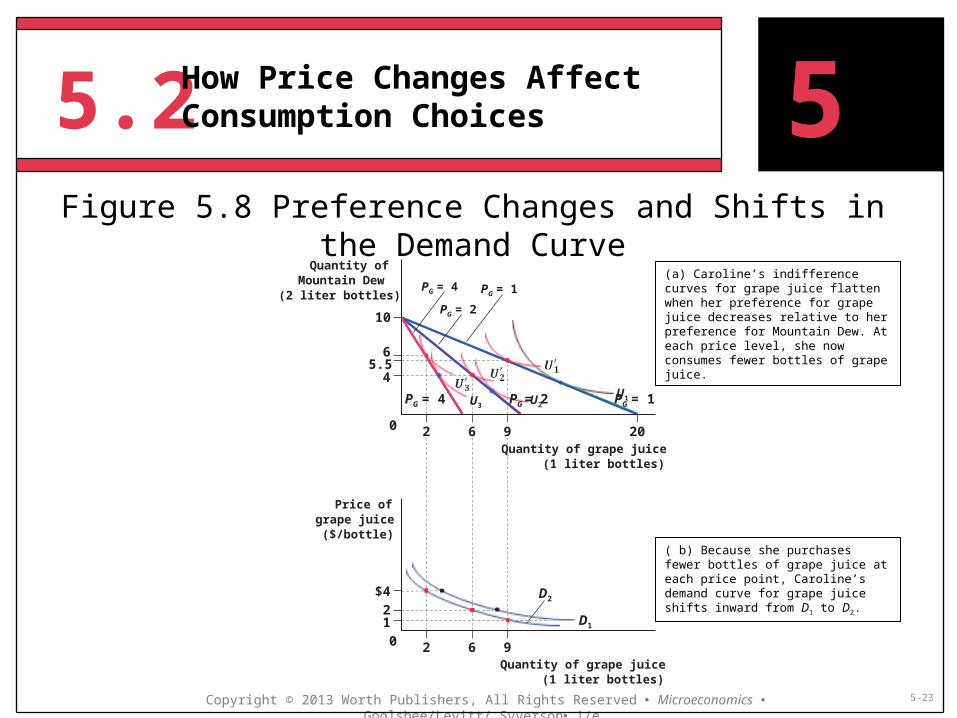
5Figure 5.8 Preference Changes and Shifts in the
Demand Curve
How Price Changes Affect Consumption Choices
Quantity ofMountain Dew(2 liter bottles)1065.54 PG = 4 PG = 2 PG = 10 2 6 9 20Quantity of grape juice(1 liter bottles)
Price ofgrape juice($/bottle)$4 D22 D110 2 6 9Quantity of grape juice(1 liter bottles)
(a) Caroline’s indifference curves for grape juice flatten when her preference for grape juice decreases relative to her preference for Mountain Dew. At each price level, she now consumes fewer bottles of grape juice.
( b) Because she purchases fewer bottles of grape juice at each price point, Caroline’s demand curve for grape juice shifts inward from D1 to D2.
PG = 4 PG = 1PG = 2
U1U3 U2
Copyright © 2013 Worth Publishers, All Rights Reserved Microeconomics Goolsbee/Levitt/ Syverson 1/e 5-24
Figure it outThe Effect of a Price change
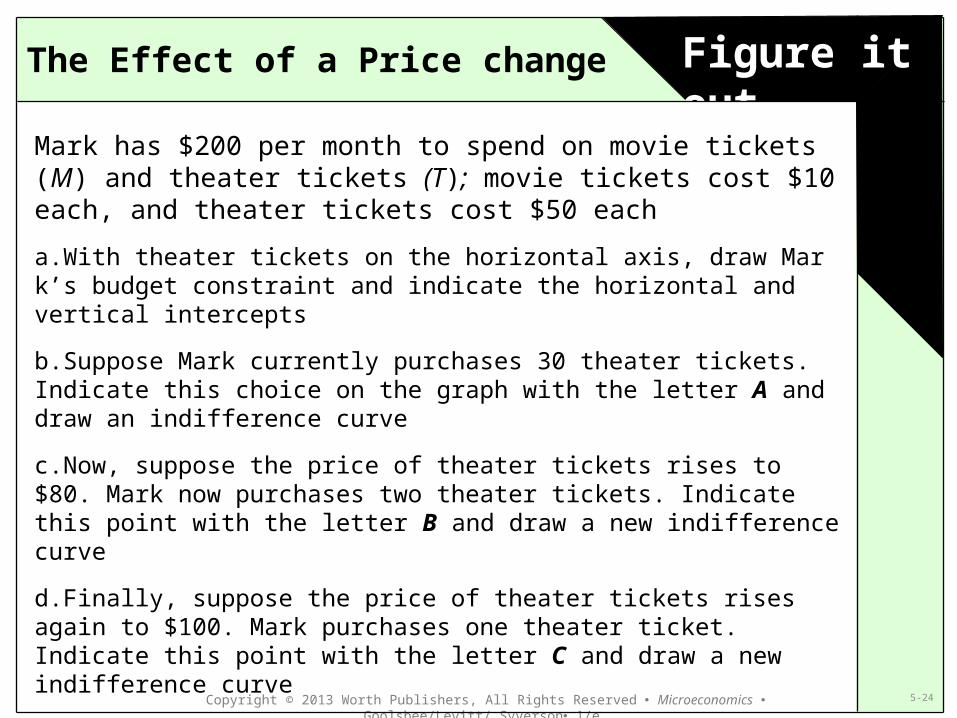
Mark has $200 per month to spend on movie tickets (M) and theater tickets (T); movie tickets cost $10 each, and theater tickets cost $50 each
a.With theater tickets on the horizontal axis, draw Mark’s budget constraint and indicate the horizontal and vertical intercepts
b.Suppose Mark currently purchases 30 theater tickets. Indicate this choice on the graph with the letter A and draw an indifference curve
c.Now, suppose the price of theater tickets rises to $80. Mark now purchases two theater tickets. Indicate this point with the letter B and draw a new indifference curve
d.Finally, suppose the price of theater tickets rises again to $100. Mark purchases one theater ticket. Indicate this point with the letter C and draw a new indifference curve
e.Draw a new diagram showing Mark’s demand curve for theater tickets

Copyright © 2013 Worth Publishers, All Rights Reserved Microeconomics Goolsbee/Levitt/ Syverson 1/e 5-25
Figure it outThe Effect of a Price change
0 1 Theater tickets
Movie tickets20
AB2 3 4
105
2.54
C
First plot the different bundles
Then the demand curve
0 1 Theater tickets
Price100
AB
2 3
50
C80
5.3
Copyright © 2013 Worth Publishers, All Rights Reserved Microeconomics Goolsbee/Levitt/ Syverson 1/e 5-26
When the price of a good changes relative to another, two things happen1.One good becomes relatively more expensive, and the other relatively less2.The total purchasing power of a consumer’s income changes
The substitution effect refers to the change in consumption choices resulting from a change in relative prices•Always negative; when the price of one good relative to another increases, consumption of the former falls, and vice versa
The income effect refers to the change in consumption choices resulting from a change in purchasing power•This is the same income effect from Section 5.1•Can be negative or positive (inferior or normal goods)
5Decomposing Consumer Responses to Price Changes into Income and Substitution Effects

5.3
Copyright © 2013 Worth Publishers, All Rights Reserved Microeconomics Goolsbee/Levitt/ Syverson 1/e 5-27
The total effect of a change in a price is the sum of the substitution and income effects•The total effect is simply the observed change in consumption of a good after a price change
5Decomposing Consumer Responses to Price Changes into Income and Substitution Effects
Effect IncomeEffecton SubstitutiEffect Total

5.3
Copyright © 2013 Worth Publishers, All Rights Reserved Microeconomics Goolsbee/Levitt/ Syverson 1/e 5-28
5Figure 5.9 The Effects of a Fall in the Price of
Restaurant Meals
Decomposing Consumer Responses to Price Changes into Income and Substitution Effects
Roundsof golf
B6Total Aeffect 5 U2
U1BC1 BC20 Restaurant3 5 mealsTotal effect

5.3
Copyright © 2013 Worth Publishers, All Rights Reserved Microeconomics Goolsbee/Levitt/ Syverson 1/e 5-29
The total effect is the sum of the substitution and income effects•The total effect is simply the observed change in consumption of a good after a price change
Isolating the Substitution Effect•Determine the bundle of goods that would have been chosen at the new price while maintaining utility experienced before the price change•To do this for a fall in the price of restaurant meals, shift the new budget constraint inward until it is tangent with the old indifference curve
5Decomposing Consumer Responses to Price Changes into Income and Substitution Effects
Effect IncomeEffecton SubstitutiEffect Total
5.3
Copyright © 2013 Worth Publishers, All Rights Reserved Microeconomics Goolsbee/Levitt/ Syverson 1/e 5-30
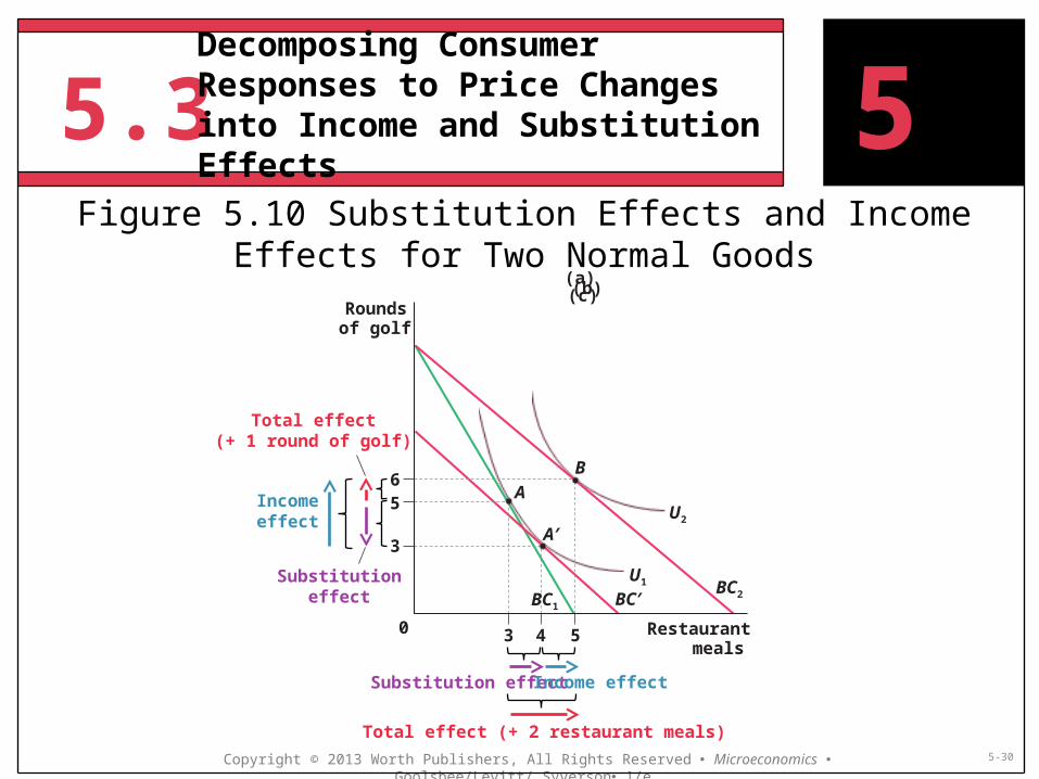
5Figure 5.10 Substitution Effects and Income Effects for
Two Normal Goods
Decomposing Consumer Responses to Price Changes into Income and Substitution Effects
(a)Roundsof golf
B6 A5 U2A′3 U1 BC2BC′BC10 Restaurant3 4 5 meals
Incomeeffect
Total effect(+ 1 round of golf)
SubstitutioneffectSubstitution effectIncome effectTotal effect (+ 2 restaurant meals)
(b)(c)
5.3
Copyright © 2013 Worth Publishers, All Rights Reserved Microeconomics Goolsbee/Levitt/ Syverson 1/e 5-31
The total effect is the sum of the substitution and income effects•The total effect is simply the observed change in consumption of a good after a price change
Isolating the Substitution Effect•Determine the bundle of goods that would have been chosen at the new price while maintaining utility experienced before the price change•For a fall in the price of restaurant meals, shift the new budget constraint inward until tangent with the old indifference curve•Restaurant meals are normal goods; therefore, the income effect is positive
Isolating the Income Effect•The income effect is the total effect minus the substitution effect
5Decomposing Consumer Responses to Price Changes into Income and Substitution Effects
Effect IncomeEffecton SubstitutiEffect Total
5.3
Copyright © 2013 Worth Publishers, All Rights Reserved Microeconomics Goolsbee/Levitt/ Syverson 1/e 5-32
Three steps to computing substitution and income effects associated with a price change. Starting with a consumer at bundle A1.Draw the new budget constraint and find the new optimal bundle (B )
• A price change for one of two goods rotates or pivots the constraint
2.Draw a line parallel to the new budget constraint, but tangent to the old indifference curve; determine the optimal bundle on the old curve associated with this theoretical budget constraint (A′)3.The substitution effect is the difference in quantities between A and A′ and the income effect is the difference in quantities between A′ and B
5Decomposing Consumer Responses to Price Changes into Income and Substitution Effects
5.3
Copyright © 2013 Worth Publishers, All Rights Reserved Microeconomics Goolsbee/Levitt/ Syverson 1/e 5-33
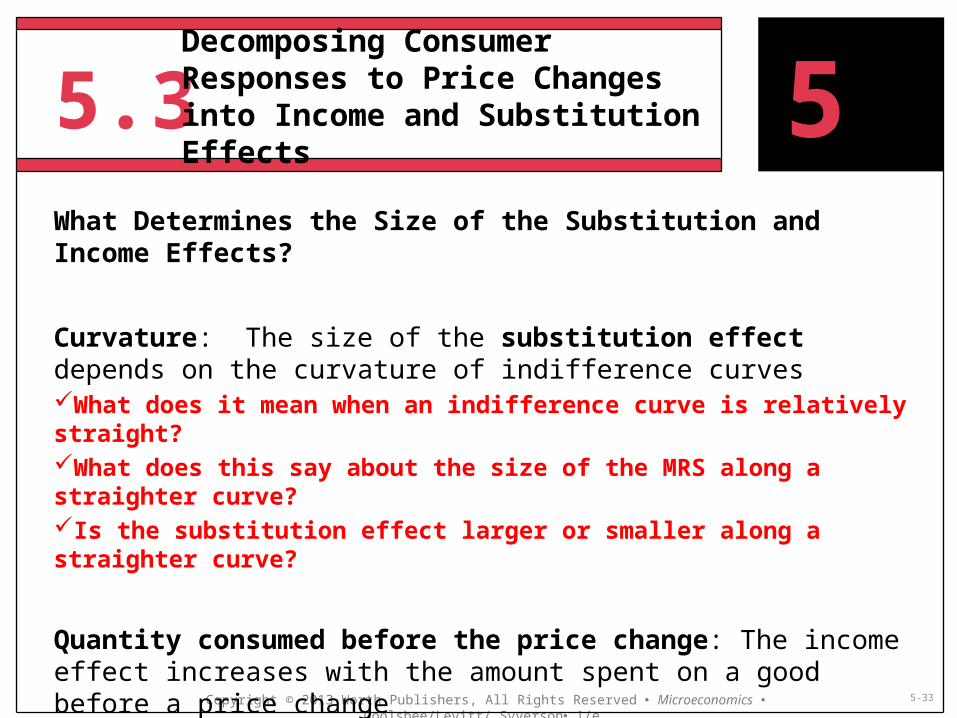
What Determines the Size of the Substitution and Income Effects?
Curvature: The size of the substitution effect depends on the curvature of indifference curvesWhat does it mean when an indifference curve is relatively straight?What does this say about the size of the MRS along a straighter curve?Is the substitution effect larger or smaller along a straighter curve?
Quantity consumed before the price change: The income effect increases with the amount spent on a good before a price changeWhy does the income effect increase with the amount spent on a good?
5Decomposing Consumer Responses to Price Changes into Income and Substitution Effects

Copyright © 2013 Worth Publishers, All Rights Reserved Microeconomics Goolsbee/Levitt/ Syverson 1/e 5-34
Figure it outThe Effect of a Price Change
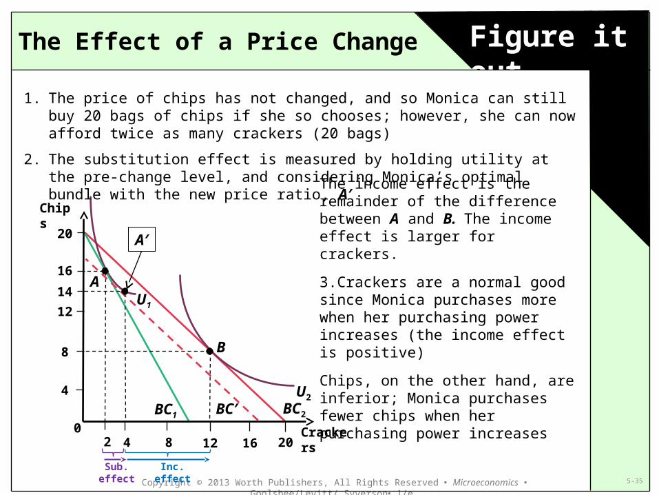
Monica eats chips and crackers. Her income is $20, and the price of chips and crackers are $1 and $2 per bag, respectively.
At these prices, she eats 16 bags of chips and two bags of crackers (point A )
When the price of crackers falls to $1, Monica consumes 8 bags of chips and 12 bags of crackers (point B )
0 4 Crackers
Chips 20Answer the following1.Why does the budget constraint rotate?2.Label your own diagram and estimate the income and substitution effects for crackers. Which is larger?3.Are crackers a normal or inferior good? Chips?
AB
8 12 16 20
161284
2
U1Total effect
Total effect
U2BC1 BC2
Copyright © 2013 Worth Publishers, All Rights Reserved Microeconomics Goolsbee/Levitt/ Syverson 1/e 5-35
Figure it outThe Effect of a Price Change
1. The price of chips has not changed, and so Monica can still buy 20 bags of chips if she so chooses; however, she can now afford twice as many crackers (20 bags)
2. The substitution effect is measured by holding utility at the pre-change level, and considering Monica’s optimal bundle with the new price ratio, A′
0 4 Crackers
Chips 20The income effect is the remainder of the difference between A and B. The income effect is larger for crackers.
3.Crackers are a normal good since Monica purchases more when her purchasing power increases (the income effect is positive)
Chips, on the other hand, are inferior; Monica purchases fewer chips when her purchasing power increases
AB
8 12 16 20
161284
2Sub. effect
U2BC1 BC2BC′
A′14
Inc. effect
U1
5.3
Copyright © 2013 Worth Publishers, All Rights Reserved Microeconomics Goolsbee/Levitt/ Syverson 1/e 5-36
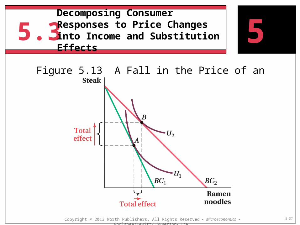
An Example of the Substitution and Income Effects for an Inferior Good
It is important to see how the income and substitution effects are opposed to one another with an inferior good.
Consider a consumer choosing bundles of steak and hamburger
5Decomposing Consumer Responses to Price Changes into Income and Substitution Effects
5.3
Copyright © 2013 Worth Publishers, All Rights Reserved Microeconomics Goolsbee/Levitt/ Syverson 1/e 5-37
Figure 5.13 A Fall in the Price of an Inferior Good
5Decomposing Consumer Responses to Price Changes into Income and Substitution Effects
5.3
Copyright © 2013 Worth Publishers, All Rights Reserved Microeconomics Goolsbee/Levitt/ Syverson 1/e 5-38
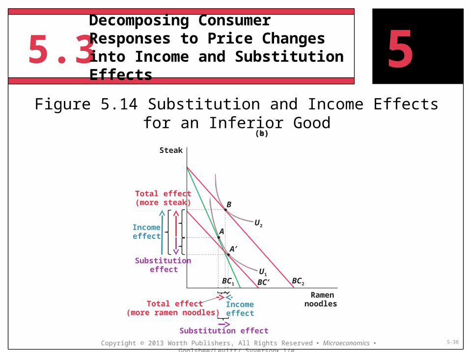
5Figure 5.14 Substitution and Income Effects for an
Inferior Good
Decomposing Consumer Responses to Price Changes into Income and Substitution Effects
(a)Steak
Total effect(more steak) BU2Income Aeffect A′Substitutioneffect U1BC1 BC2BC′ RamenIncomeTotal effect noodleseffect(more ramen noodles)
Substitution effect
(b)(c)
Application
Copyright © 2013 Worth Publishers, All Rights Reserved Microeconomics Goolsbee/Levitt/ Syverson 1/e 5-39
5
Citation: Shogren, J. F., Shin, S. Y., Hayes, D. J., and Kliebenstein, J. B. 1994. “Resolving Differences in Willingness to Pay and Willingness To Accept.” The American Economic Review 84(1): 255-270.
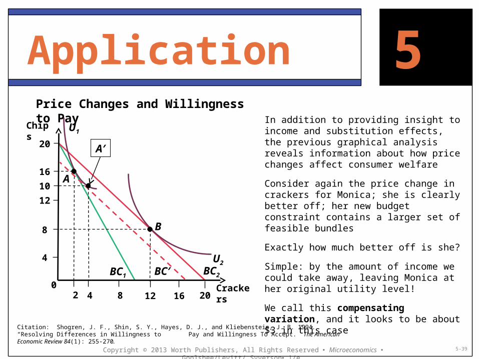
Price Changes and Willingness to Pay In addition to providing insight to income
and substitution effects, the previous graphical analysis reveals information about how price changes affect consumer welfare
Consider again the price change in crackers for Monica; she is clearly better off; her new budget constraint contains a larger set of feasible bundles
Exactly how much better off is she?
Simple: by the amount of income we could take away, leaving Monica at her original utility level!
We call this compensating variation, and it looks to be about $3 in this case
0 4 Crackers
Chips 20A
B
8 12 16 20
161284
2U2BC1 BC2BC′
A′10
U1

Application
Copyright © 2013 Worth Publishers, All Rights Reserved Microeconomics Goolsbee/Levitt/ Syverson 1/e 5-40
Price Changes and Willingness to Pay
Monica should be willing to pay $3 to experience a lower price on crackers, and she should be willing to accept $3 in lieu of the price change
The theoretical equivalency between willingness to pay (WTP) and willingness to accept (WTA) extends to quantity differences
In practice, however, WTA for a product a consumer currently owns generally exceeds WTP for that same product
Images: FreeDigitalPhotos.net
5
Citation: Shogren, J. F., Shin, S. Y., Hayes, D. J., and Kliebenstein, J. B. 1994. “Resolving Differences in Willingness to Pay and Willingness To Accept.” The American Economic Review 84(1): 255-270.

Application
Copyright © 2013 Worth Publishers, All Rights Reserved Microeconomics Goolsbee/Levitt/ Syverson 1/e 5-41
5
Citation: Shogren, J. F., Shin, S. Y., Hayes, D. J., and Kliebenstein, J. B. 1994. “Resolving Differences in Willingness to Pay and Willingness To Accept.” The American Economic Review 84(1): 255-270.
Images: FreeDigitalPhotos.net
5.3
Copyright © 2013 Worth Publishers, All Rights Reserved Microeconomics Goolsbee/Levitt/ Syverson 1/e 5-42
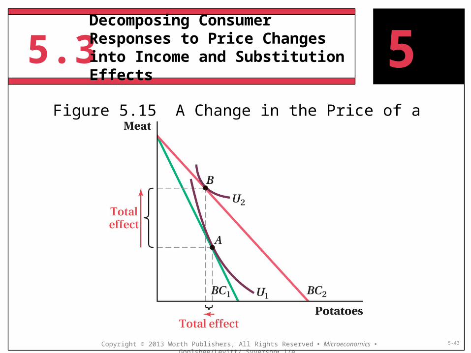
Giffen goods are goods for which quantity demanded increases as price rises•Inferior goods, but the income effect outweighs the substitution effect•Results in an upward sloping demand curve
When the price of a Giffen good drops, the substitution effect (which acts to increase demand) is smaller than the income effect
Economists sometimes question whether Giffen goods actually exist•The few examples with humans tend to focus on very poor households and commodity crops (e.g., rice and potatoes)
5Decomposing Consumer Responses to Price Changes into Income and Substitution Effects
5.3
Copyright © 2013 Worth Publishers, All Rights Reserved Microeconomics Goolsbee/Levitt/ Syverson 1/e 5-43
Figure 5.15 A Change in the Price of a Giffen Good
5Decomposing Consumer Responses to Price Changes into Income and Substitution Effects

Application
Copyright © 2013 Worth Publishers, All Rights Reserved Microeconomics Goolsbee/Levitt/ Syverson 1/e 5-44
Rats, Quinine, and Giffen Behavior
Battalio, et al. (1990) found existence of Giffen behavior in rats using quinine solution (tonic water) and root beer•Rats prefer root beer to water, and water to quinine solution
Rats were given limited “lever-pulls” to release liquid, and root beer pulls released less liquid than the quinine pull (no water was available during the experiment)
Findings imply quinine solution is a Giffen good for rats•First, quinine solution was shown to be an inferior good (negative income effect)•Second, when the price of quinine solution was lowered (more volume per pull), the average rat reduced volumetric consumption, shifting to root beer instead
Images: FreeDigitalPhotos.net
5
Citation: Battalio, R. C., Kagel, J. H., and Kogut, C. A. 1991. “Experimental Confirmation of the Existence of a Giffen Good.” The American Economic Review 81(4): 961-970.

5.4
Copyright © 2013 Worth Publishers, All Rights Reserved Microeconomics Goolsbee/Levitt/ Syverson 1/e 5-45
A Change in the Price of a Substitute Good
When the price of a substitute good increases, we expect consumption of the primary good to increase•Consider Pepsi-Cola and Coca-Cola
5The Impact of Changes in Another Good’s Price: Substitutes and Complements

5.4
Copyright © 2013 Worth Publishers, All Rights Reserved Microeconomics Goolsbee/Levitt/ Syverson 1/e 5-46
5The Impact of Changes in Another Good’s Price: Substitutes and Complements
0 4
Pepsi
Coke
20 A
B8 12 16 20
161284
U1
U2 BC1BC2
Pepsi consumption falls
Coke consumption rises
At original prices, this consumer purchases 16 bottles of Pepsi and 4 bottles of Coke
When the price of Pepsi doubles, Coke consumption increases by 200% (to 12 bottles), and Pepsi consumption falls by 75% (to 4 bottles)
Coke consumption rose when the price of Pepsi rose: they are substitutes
Figure 5.17 When the Price of a Substitute Rises, Demand Rises

5.4
Copyright © 2013 Worth Publishers, All Rights Reserved Microeconomics Goolsbee/Levitt/ Syverson 1/e 5-47
A Change in the Price of a Substitute Good
When the price of a substitute good increases, we expect consumption of the primary good to increase•Consider Pepsi-Cola and Coca-Cola
When the price of a complement increases, we expect consumption of the primary good to decrease•Consider tortilla chips and salsa
5The Impact of Changes in Another Good’s Price: Substitutes and Complements
5.4
Copyright © 2013 Worth Publishers, All Rights Reserved Microeconomics Goolsbee/Levitt/ Syverson 1/e 5-48
5The Impact of Changes in Another Good’s Price: Substitutes and Complements
04
Salsa
Chips
10
AB
8 12 16 20
8
6
4
2U1U2
BC1
BC2
Chip price doubles
Salsa consumption falls
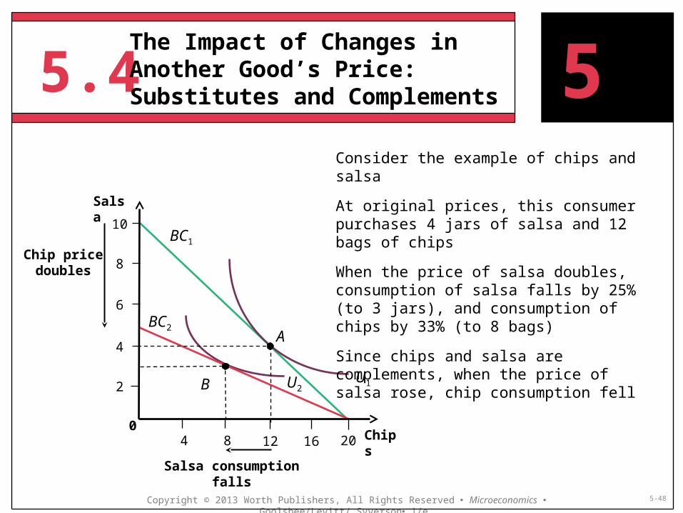
Consider the example of chips and salsa
At original prices, this consumer purchases 4 jars of salsa and 12 bags of chips
When the price of salsa doubles, consumption of salsa falls by 25% (to 3 jars), and consumption of chips by 33% (to 8 bags)
Since chips and salsa are complements, when the price of salsa rose, chip consumption fell

5.4
Copyright © 2013 Worth Publishers, All Rights Reserved Microeconomics Goolsbee/Levitt/ Syverson 1/e 5-49
A Change in the Price of a Substitute Good
When the price of a substitute good increases, we expect consumption of the primary good to increase•Consider Pepsi-Cola and Coca-Cola
When the price of a complement increases, we expect consumption of the primary good to decrease•Consider tortilla chips and salsa
These relationships help to explain the shifts in demand examined in Chapter 2
5The Impact of Changes in Another Good’s Price: Substitutes and Complements
5.4
Copyright © 2013 Worth Publishers, All Rights Reserved Microeconomics Goolsbee/Levitt/ Syverson 1/e 5-50
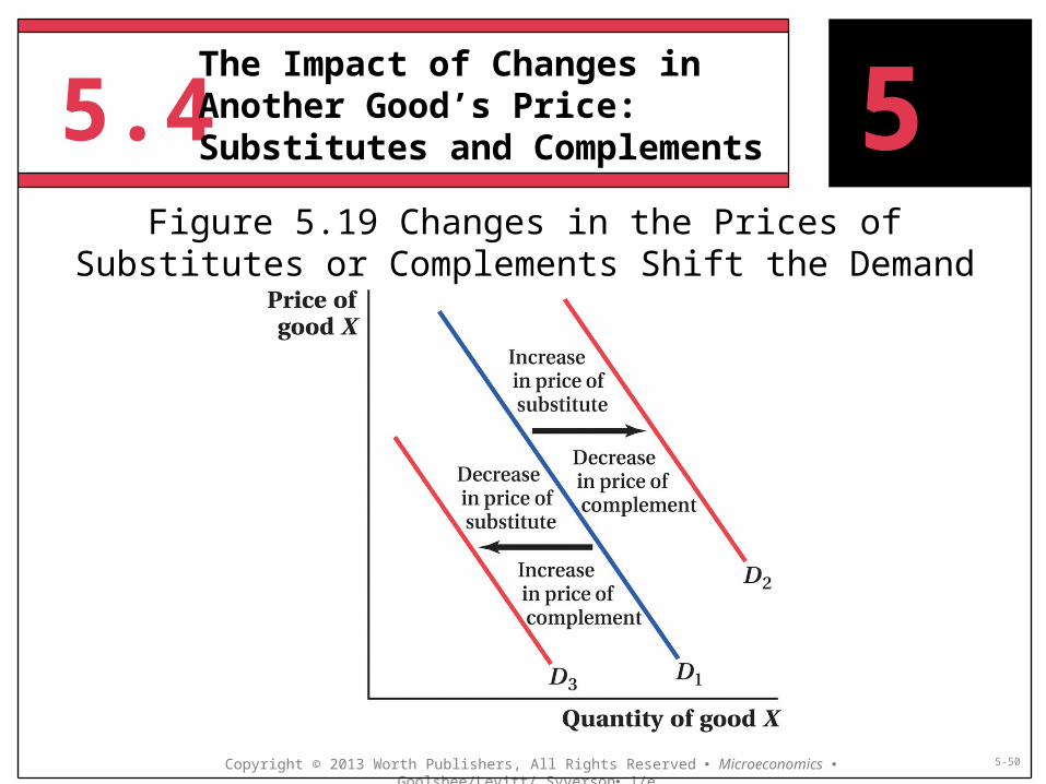
Figure 5.19 Changes in the Prices of Substitutes or Complements Shift the Demand Curve
5The Impact of Changes in Another Good’s Price: Substitutes and Complements

5.5
Copyright © 2013 Worth Publishers, All Rights Reserved Microeconomics Goolsbee/Levitt/ Syverson 1/e 5-51
The final step linking consumer theory to market demand is probably the easiest•Market demand is the horizontal sum of individual demand curves•The market quantity demanded at each price is the sum of the individual quantities demanded at each price•The market demand curve is found by summing horizontally individual demand curves
Consider the market for scooters
5Combining Individual Demand Curves to Obtain the Market Demand Curve

5.5
Copyright © 2013 Worth Publishers, All Rights Reserved Microeconomics Goolsbee/Levitt/ Syverson 1/e 5-52
5Figure 5.21 The Market Demand Curve
Combining Individual Demand Curves to Obtain the Market Demand Curve
(a)B
ADmarket =Dyou + Dcousin
6 12
(b)
Dcousin8
Price($/scooter)$524020
Dyou0 3 Quantity of scooters4
(c)
5.5
Copyright © 2013 Worth Publishers, All Rights Reserved Microeconomics Goolsbee/Levitt/ Syverson 1/e 5-53
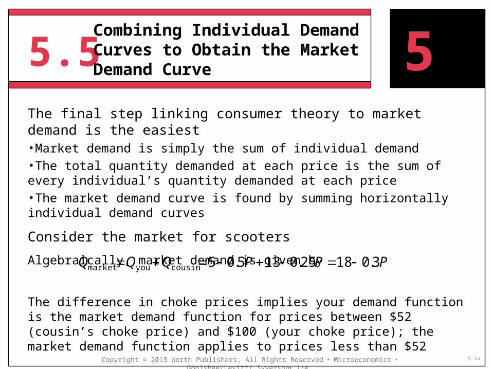
The final step linking consumer theory to market demand is the easiest•Market demand is simply the sum of individual demand•The total quantity demanded at each price is the sum of every individual’s quantity demanded at each price•The market demand curve is found by summing horizontally individual demand curves
Consider the market for scooters
Algebraically, market demand is given by
The difference in choke prices implies your demand function is the market demand function for prices between $52 (cousin’s choke price) and $100 (your choke price); the market demand function applies to prices less than $52
5Combining Individual Demand Curves to Obtain the Market Demand Curve
PPPQQQ 3.01825.0135.05cousinyoumarket
Copyright © 2013 Worth Publishers, All Rights Reserved Microeconomics Goolsbee/Levitt/ Syverson 1/e 5-54
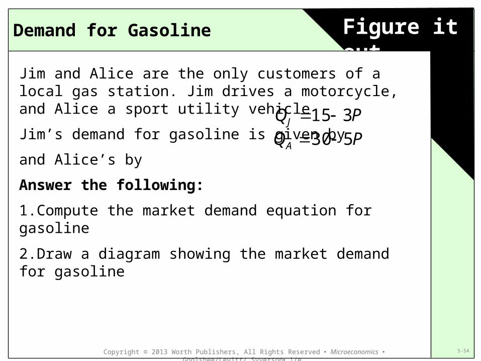
Figure it outDemand for Gasoline
Jim and Alice are the only customers of a local gas station. Jim drives a motorcycle, and Alice a sport utility vehicle
Jim’s demand for gasoline is given by
and Alice’s by
Answer the following:
1.Compute the market demand equation for gasoline
2.Draw a diagram showing the market demand for gasoline
PQJ 315 PQA 530
Copyright © 2013 Worth Publishers, All Rights Reserved Microeconomics Goolsbee/Levitt/ Syverson 1/e 5-55
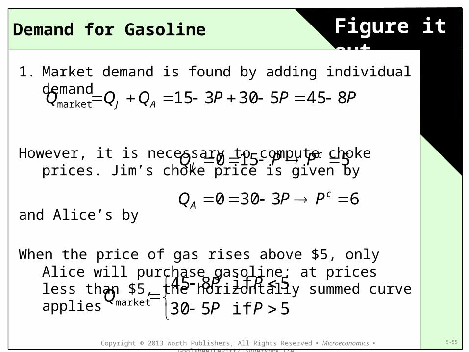
Figure it outDemand for Gasoline
1. Market demand is found by adding individual demand
However, it is necessary to compute choke prices. Jim’s choke price is given by
and Alice’s by
When the price of gas rises above $5, only Alice will purchase gasoline; at prices less than $5, the horizontally summed curve applies
PPPQQQ AJ 845530315market
63300 cA PPQ
5150 cJ PPQ
5 if 530
5 if 845market PP
PPQ

Copyright © 2013 Worth Publishers, All Rights Reserved Microeconomics Goolsbee/Levitt/ Syverson 1/e 5-56
Figure it outDemand for Gasoline
2. The market demand curve
0 8 Gallons
Price6
16 24 32 40
534
Dmarket48
12
5

5.6 Conclusion
Copyright © 2013 Worth Publishers, All Rights Reserved Microeconomics Goolsbee/Levitt/ Syverson 1/e 5-57
This chapter concludes our in-depth analysis of the consumer side of the supply and demand model. We•Examined how income and prices affect consumer choices•Made the link between consumer theory and market demand
In Chapter 6 we begin a parallel in-depth examination of producer behavior
5