individual preferences, monetary gambles, and stock market...

Individual Preferences, Monetary Gambles, and Stock MarketParticipation: A Case for Narrow Framing

By NICHOLAS BARBERIS, MING HUANG, AND RICHARD H. THALER*

We argue that “narrow framing,” whereby an agent who is offered a new gambleevaluates that gamble in isolation, may be a more important feature of decision-making than previously realized. Our starting point is the evidence that people areoften averse to a small, independent gamble, even when the gamble is actuariallyfavorable. We find that a surprisingly wide range of utility functions, including manynonexpected utility specifications, have trouble explaining this evidence, but thatthis difficulty can be overcome by allowing for narrow framing. Our analysis makespredictions as to what kinds of preferences can most easily address the stock marketparticipation puzzle. (JEL D81, G11)

Economists, and financial economists in par-ticular, have long been interested in how peopleevaluate risk. In this paper, we try to shed newlight on this topic. Specifically, we argue that afeature known as “narrow framing” may play amore important role in decision-making underrisk than previously realized. In traditionalmodels, which define utility over total wealth orconsumption, an agent who is offered a newgamble evaluates that gamble by merging itwith the other risks she already faces and check-ing whether the combination is attractive. Nar-row framing, by contrast, occurs when an agentwho is offered a new gamble evaluates that

gamble to some extent in isolation, separatelyfrom her other risks.

Our starting point is the evidence that peopleare often reluctant to take a small, independentgamble, even when the gamble is actuariallyfavorable. For example, in an experimental set-ting, Amos Tversky and Daniel Kahneman(1992) find that approximately half of their sub-jects turn down a small gamble with twoequiprobable outcomes, even though the poten-tial gain is twice the potential loss.

In this paper, we try to understand what kindsof preferences can explain such attitudes to risk.It is already understood that, without a propertyknown as “first-order” risk aversion, it is hard forpreferences to explain the rejection of a small,independent, actuarially favorable gamble (LarryG. Epstein and Stanley E. Zin, 1990; MatthewRabin, 2000). Our own contributions are: first, toshow that, surprisingly, even utility functions thatdo exhibit first-order risk aversion have difficultyexplaining why such a gamble would be rejected;and, second, that utility functions that combinefirst-order risk aversion with narrow framing havea much easier time doing so.1

The intuition for these results is straightforward.

* Barberis: Yale School of Management, 135 ProspectStreet, P.O. Box 208200, New Haven, CT 06520 (e-mail:[email protected]); Huang: Johnson School ofManagement and SUFE, Sage Hall, Cornell University,Ithaca, NY 14853 (e-mail: [email protected]); Thaler:Graduate School of Business, University of Chicago, 5807South Woodlawn Avenue, Chicago, IL 60637 (e-mail:[email protected]). Huang acknowledges finan-cial support from the National Natural Science Foundation ofChina under grant 70432002. We thank three anonymousreferees, Douglas Bernheim, John Campbell, Darrell Duffie,Larry Epstein, John Heaton, Daniel Kahneman, David Laib-son, Erzo Luttmer, Terrance Odean, Mark Rubinstein, BillSharpe, Jeffrey Zwiebel, and seminar participants at DukeUniversity, Emory University, Harvard University, INSEAD,London Business School, London School of Economics, Mas-sachusetts Institute of Technology, New York University,Northwestern University, Princeton University, Stanford Uni-versity, University of California at Berkeley, University ofChicago, University of Pennsylvania, Yale University, and theNBER for helpful comments.

1 We give the formal definition of first-order risk aver-sion in Section I. In informal terms, a utility functionexhibits first-order risk aversion if it is locally risk averse,unlike most standard preferences, which are locally risk-neutral; loss aversion, whereby the utility function is kinkedat the current wealth level, is an example of first-order riskaversion.

1069

Suppose that an agent with first-order risk aver-sion, but who does not engage in narrow fram-ing, is offered a small, independent, actuariallyfavorable gamble. Suppose also, as is reason-able, that the agent faces some preexisting risk,such as labor income risk or house price risk. Inthe absence of narrow framing, the agent mustevaluate the new gamble by merging it with herpreexisting risk and checking if the combinationis attractive. It turns out that the combination isattractive: since the new gamble is independentof the agent’s other risks, it diversifies thoseother risks, and, even though first-order riskaverse, the agent finds this useful. The onlyway to make the agent reject the gamble is tochoose an extreme parameterization of herutility function. However, such a parameter-ization typically implies, counterfactually, therejection of highly attractive gambles withlarger stakes.

A simple way out of this difficulty, then, is tosuppose that, when the agent evaluates the smallgamble, she does not fully merge it with herpreexisting risk but, rather, thinks about it inisolation, to some extent; in other words, sheframes the gamble narrowly. Using a recentlydeveloped preference specification that allowsfor both first-order risk aversion and narrowframing, we confirm that a utility function withthese features can easily explain the rejection of asmall, independent, actuarially favorable gamble,while also making sensible predictions about atti-tudes to large-scale gambles: if the agent’s first-order risk aversion is focused directly on the smallgamble rather than just on overall wealth risk, shewill be reluctant to take it.

Our analysis of independent monetary gam-bles has useful implications for financial mar-kets. For example, it is useful for understandingwhat kinds of preferences can address the stockmarket participation puzzle: the fact that, eventhough the stock market has a high mean returnand a low correlation with other householdrisks, many households have historically beenreluctant to allocate any money to it (N. Greg-ory Mankiw and Stephen P. Zeldes, 1991; Mi-chael Haliassos and Carol C. Bertaut, 1995).

It is already understood that, without first-order risk aversion, it is hard to find a preference-based explanation of this evidence. Our analysisof small, independent gambles suggests a moresurprising prediction: even preferences that do ex-hibit first-order risk aversion will have trouble

explaining nonparticipation. It also suggests thatpreferences that combine first-order risk aversionwith narrow framing—in this case, narrow fram-ing of stock market risk—will have an easier timedoing so. We confirm these predictions in a simpleportfolio choice setting.

While the term “narrow framing” was firstused by Kahneman and Daniel Lovallo (1993),the more general concept of “decision framing”was introduced much earlier by Tversky andKahneman (1981). There are already severalcleverly designed laboratory demonstrations ofnarrow framing in the literature.2 This papershows that a more basic piece of evidence onattitudes to risk, not normally associated withnarrow framing, may also need to be thought ofin these terms. Moreover, while existing exam-ples of narrow framing do not always haveobvious counterparts in the everyday risks peo-ple face, the simple risks we consider do—notleast in stock market risk—making our resultsapplicable in a variety of contexts.

The idea that a combination of first-order riskaversion and narrow framing may be relevantfor understanding aversion to small gambles hasbeen proposed before, most notably by Rabinand Thaler (2001). Those authors do not, how-ever, demonstrate the sense in which first-orderrisk aversion, on its own, is insufficient. This isthe crucial issue we tackle here.

If narrow framing does, sometimes, play arole in the way people evaluate risk, it is im-portant that we learn more about its underlyingcauses. At the end of the paper, we discuss someinterpretations of narrow framing, including thepossibility that it arises when people make de-cisions intuitively, rather than through effortfulreasoning (Kahneman, 2003). We argue that therecent attempts to outline a theory of narrowframing have made framing-based hypothesesmuch more testable than they were before.

I. Attitudes to Monetary Gambles

People are often averse to a small, indepen-dent gamble, even when the gamble is actuari-ally favorable. In an experimental setting,Tversky and Kahneman (1992) find that ap-

2 Daniel Read et al. (1999) survey many examples ofnarrow framing, including those documented by Tverskyand Kahneman (1981) and Donald A. Redelmeier and Tver-sky (1992).

1070 THE AMERICAN ECONOMIC REVIEW SEPTEMBER 2006

proximately half of their subjects turn down asmall gamble with two equiprobable outcomes,even though the potential gain is twice the po-tential loss. In a more recent study, MohammedAbdellaoui et al. (2005) also find that theirmedian subject is indifferent to a small gamblewith two equiprobable outcomes only when thegain is twice the potential loss.3

In this paper, we try to understand what kindsof preferences can explain an aversion to asmall, independent, actuarially favorable gam-ble. For concreteness, we consider a small, in-dependent gamble whose potential gain is muchless than twice the potential loss, namely4

GS � �550, 1⁄2 ; �500, 1⁄2 �,

to be read as “gain $550 with probability 1⁄2 andlose $500 with probability 1⁄2 ,” and ask: whatkinds of preferences can explain the rejection ofthis gamble? We do not insist that a utilityfunction be able to explain the rejection of GS atall wealth levels, but rather that it do so over arange of wealth levels—at wealth levels below$1 million, say. We take “wealth” to mean totalwealth, including both financial assets and suchnonfinancial assets as human capital.

Is it reasonable to posit that individuals tendto reject GS even at a wealth level of $1 million,a wealth level that probably exceeds that ofTversky and Kahneman’s (1992) median sub-ject? In Barberis et al. (2003), an earlier versionof the current paper, we ask four groups ofpeople—68 part-time MBA students, 30 finan-cial advisors, 19 chief investment officers atlarge asset management firms, and 34 clients ofa U.S. bank’s private wealth management divi-sion (the median wealth in this last group ex-

ceeds $10 million)—about their attitudes to ahypothetical GS. In all four groups, the majorityreject GS, and even in the wealthiest group, therejection rate is 71 percent. Playing GS for realmoney with a second group of MBA studentsleads to an even higher rejection rate thanamong the first group of MBAs.

We focus on preference-based explanationsfor aversion to small gambles because the alter-native explanations seem incomplete. One alter-native view is that the rejection of gambles likeGS is due to transaction costs that might beincurred if a liquidity-constrained agent has tofinance a loss by selling illiquid assets (RajChetty, 2004). Such a mechanism does not,however, explain why wealthy subjects withsubstantial liquid assets are often averse to GS.Nor is suspicion a satisfactory explanation forthe rejection of GS: the fear, for example, thatthe experimenter is using a biased coin to de-termine the outcome. Offering to use a subject’scoin instead does little to change attitudes to thegamble.5

Of course, many utility functions can capture anaversion to GS by simply assuming high risk aver-sion. To ensure that the assumed risk aversion isrealistic, we insist that the utility functions weconsider also make sensible predictions about at-titudes to large-scale gambles by, for example,predicting acceptance of the large, independentgamble6

GL � �20,000,000, 1⁄2 ; �10,000, 1⁄2 �

over a reasonable range of wealth levels—wealth levels above $100,000, say.

In summary, then, we are interested in under-standing what kinds of preference specificationscan predict both:

I. That GS is rejected for wealth levels W �$1,000,000; and

II. That GL is accepted for wealth levels W �$100,000.

3 This evidence is not necessarily inconsistent with risk-seeking behavior like casino gambling or the buying oflottery tickets. Lottery tickets are different from Tverskyand Kahneman’s (1992) gambles, in that they offer a tinyprobability of substantial gain, rather than two equiprobableoutcomes. An individual can be averse to a 50:50 betoffering a gain against a loss, even if she is risk-seekingover low-probability gains. Gambling is a special phenom-enon, in that people would not accept the terms of tradeoffered at a casino if those terms were offered by their bank,say. It must be that, in the casino setting, people eithermisestimate their chance of winning or receive utility fromthe gambling activity itself.

4 The “S” subscript in GS stands for Small stakes. Wesometimes use the notation X/Y to refer to a 50:50 bet to win$X or lose $Y. GS is therefore a “550/500” bet.

5 It is also unlikely that people turn down GS simplybecause they do not want, or feel able, to evaluate it. Inour experience, subjects, when debriefed, typically ex-plain their aversion to GS by saying that “the pleasure ofa $550 gain doesn’t compensate for the pain of a $500loss.” It therefore appears that they do evaluate the gamble,but find it unattractive.

6 The “L” subscript in GL stands for Large stakes.

1071VOL. 96 NO. 4 BARBERIS ET AL.: A CASE FOR NARROW FRAMING

For certain utility specifications, it can makea difference whether gambles are “immediate”or “delayed.” A gamble is immediate if its un-certainty is resolved at once, before any furtherconsumption decisions are made. A delayedgamble, on the other hand, might play out asfollows: in the case of GS, the subject is toldthat, at some point in the next few months, shewill be contacted and informed either that shehas just won $550 or that she has lost $500, thetwo outcomes being equally probable and inde-pendent of other risks.

Although certain utility functions can predictdifferent attitudes to immediate and delayed gam-bles, people do not appear to treat the two kinds ofbets very differently. Barberis et al. (2003), forexample, record very similar rejection rates forimmediate and delayed versions of GS. We there-fore look for preference specifications that cansatisfy conditions I and II both when GS and GLare immediate, and when they are delayed. Sincea delayed gamble’s uncertainty is resolved onlyafter today’s consumption is set, it must be ana-lyzed in a multiperiod framework. We thereforework with intertemporal preferences, not staticones, throughout the paper.

A. Utility Functions

To structure our discussion, we introduce asimple taxonomy of intertemporal preferences.Our list is not exhaustive, but it covers most of thepreference specifications used in economics. Inparentheses, we list the abbreviations that we useto refer to specific classes of utility functions.

[EU]: Expected utility preferences

Nonexpected utility preferences:

[R-EU]: Recursive utility with EUcertainty equivalent

[R-SORA]: Recursive utility with non-EU,second-order risk aversecertainty equivalent

[R-FORA]: Recursive utility with non-EU,first-order risk averse certaintyequivalent

Expected utility preferences are familiarenough. In an intertemporal setting, nonex-pected utility is typically implemented using a

recursive structure in which time t utility, Vt,is defined through

(1) Vt � W�Ct , ��Vt � 1�It ��,

where �(Vt�1�It) is the certainty equivalent ofthe distribution of future utility Vt�1 condi-tional on time t information It, and W( � , � ) is anaggregator function which aggregates currentconsumption Ct with the certainty equivalent offuture utility to give current utility.

The three kinds of recursive utility on our listdiffer in the properties they impose on the cer-tainty equivalent functional ��. In the firstkind, labelled “R-EU,” �� has the expectedutility form, so that

(2) ��X� � h�1Eh�X�,

for some increasing h�. In the “R-SORA”class, �� is non-EU but exhibits “second-order” risk aversion, which means that it pre-dicts risk neutrality for infinitesimal risks. Insimple terms, utility functions with second-or-der risk aversion are smooth. Finally, we con-sider the “R-FORA” class, in which �� isnon-EU and exhibits “first-order” risk aversion,which, as noted earlier, means that it predictsrisk aversion even over infinitesimal bets.7

II. The Limitations of Standard Preferences

It is already understood that the first threekinds of utility functions on our list—the EU,R-EU, and R-SORA classes—have trouble sat-isfying condition I (the rejection of GS) whilealso satisfying condition II (the acceptance ofGL). Rabin (2000), for example, shows that noincreasing, concave utility function in the EUclass is consistent with both conditions. Theintuition is straightforward. An individual withEU preferences is locally risk-neutral; since GS

7 The labels “second-order” and “first-order” are due toUzi Segal and Avia Spivak (1990). Formally, second-orderrisk aversion means that the premium paid to avoid anactuarially fair gamble k� is, as k 3 0, proportional to k2.Under first-order risk aversion, the premium is proportionalto k. While non-EU functions can exhibit either first- orsecond-order risk aversion, utility functions in the EU classcan generically exhibit only second-order risk aversion: anincreasing, concave utility function can have a kink only ata countable number of points.


involves small stakes, she would normally takeit. To get her to reject it, in accordance withcondition I, we need very high local curvature.In fact, her utility function must have high localcurvature at all wealth levels below $1 millionbecause condition I requires rejection of GS atall points in that range. Rabin’s (2000) analysisshows that “linking” these locally concavepieces gives a utility function with global riskaversion so high that the agent rejects even thevery favorable large gamble GL.

While R-EU preferences are nonexpectedutility, the fact that, in this case, the certaintyequivalent functional �� is in the expectedutility class means that an agent with thesepreferences evaluates risk using an expectedutility function. Rabin’s (2000) argument there-fore also applies to R-EU preferences: no utilityfunction in this class is consistent with bothconditions I and II.

R-SORA preferences can, in principle, satisfyconditions I and II, but only with difficulty. Anagent with R-SORA preferences is locally risk-neutral and will therefore normally be happy toaccept a small, actuarially favorable gamble likeGS. To make her reject it, we need very high localcurvature, which, in turn, requires an extreme pa-rameterization. Such a parameterization, however,almost always implies high global risk aversion,thereby making the individual reject attractive,large-scale gambles like GL.8

The main contribution of this paper is toshow that even the fourth preference class onour list—the R-FORA class, in which the cer-tainty equivalent functional �� is non-EU andfirst-order risk averse—has difficulty satisfyingconditions I and II. This is a surprising resultbecause, at first sight, it appears that R-FORApreferences can easily be consistent with theseconditions. In fact, as noted by Andrew Ang etal. (2005) and anticipated even earlier by Ep-stein and Zin (1990), such preferences have notrouble satisfying conditions I and II, so long as

the gambles are played out immediately, a ca-veat that will turn out to be critical.

To see what happens when the gambles areimmediate, consider the following R-FORApreferences:

(3) W�C, �� 1 � ��C� ��1/�,

0 � � 1,

where �� takes a form developed by Faruk Gul(1991),

(4) ��V�1 � � � E�V1 � �� 1�

� E��V1 � � � ��V�1 � ��1�V � ��V��,

0 � � 1, � 1.

These preferences are often referred to as “dis-appointment aversion” preferences: the agentincurs disutility if the outcome of V falls belowthe certainty equivalent �(V). The parameter governs the degree of disutility, in other words,how sensitive the agent is to losses as opposedto gains. A � 1 puts a kink in the utilityfunction at the certainty equivalent point,thereby generating first-order risk aversion.

Epstein and Zin (1989), who give a carefulexposition of recursive utility, propose that, toevaluate an immediate gamble v at time �, anagent with the recursive preferences in (1) in-serts an infinitesimal time step �� immediatelybefore time � consumption C� is chosen, andthen applies the recursive calculation over thistime step, checking whether the utility fromtaking the gamble,

(5) W�0, ��V� � �� W�0, ��J�W� � ��

� W�0, ��J�W� v��,

where J� is the agent’s value function at time� � ��, is greater than the utility from nottaking the gamble,

(6) W�0, ��V� � �� W�0, ��J�W� � ��

� W�0, ��J�W� ��.

The decision therefore comes down to compar-ing �(J(W� � v)) and �(J(W�)).

8 Those R-SORA preferences that are able to satisfyconditions I and II typically stumble on the following ad-ditional observation: that people tend to reject 1.1y/y andaccept 4y/y for a wide range of values of y. R-SORApreferences find it hard to explain such “linear” attitudes, asthey need to invoke very strong nonlinearity, or local cur-vature, to capture the rejection of 1.1y/y for just one value ofy. For more discussion of EU, R-EU, and R-SORA prefer-ences, see Barberis et al. (2003).


Suppose that, aside from v, the agent’s otherinvestment opportunities are i.i.d. across peri-ods, and that the outcome of v is independent of,and does not affect, these other opportunities. Itis then straightforward to show that, for t � � ��, the time t value function in the case of(3)–(4) takes the form

(7) J�Wt � � AWt

for some constant A. Equations (5) and (6)immediately imply that the agent evaluates vby comparing �(W� � v) and �(W�). Bytaking v to be GS or GL, we see that thepreferences in (3)–(4) can satisfy conditionsI and II in the case of immediate gambles,so long as there are values of � and forwhich

(8) ��W� 550�1 � � �W� � 500�1 � ��1/�1 � ��

� �1 �1/�1 � ��W�

holds for all wealth levels below $1 million, and

(9) ��W� 20,000,000�1 � �

�W� � 10,000�1 � ��1/�1 � ��

� �1 �1/�1 � ��W�

holds for all wealth levels above $100,000. Aquick calculation confirms that (�, ) � (2, 2)satisfies both (8) and (9). Since controls sen-sitivity to losses relative to sensitivity to gains,we need � 1.1 so that the 550/500 bet, with its1.1 ratio of gain to loss, is rejected.

The intuition for why R-FORA preferencescan explain attitudes to GS and GL when thesegambles are played out immediately is straight-forward. In the case of EU, R-EU, and R-SORApreferences, the difficulty is that the agent islocally risk-neutral, forcing us to push risk aver-sion over large gambles up to dramatically highlevels in order to explain the rejection of GS, the550/500 bet. An agent with R-FORA prefer-ences is, by definition, locally risk averse. Riskaversion over large gambles does not, therefore,need to be increased very much to ensure thatGS is rejected.

In the special case where GS and GL are playedout immediately, then, preferences with first-orderrisk aversion can satisfy conditions I and II. Wenow show that, in the more realistic and generalsetting where the gambles are played out withsome delay, even preferences with first-order riskaversion have a hard time satisfying these condi-tions. In particular, while they can easily explainaversion to small, immediate gambles, theyhave great difficulty—in a sense that we makeprecise—capturing aversion to small, delayedgambles. This is a serious concern because, asnoted in Section I, people are just as averse tothe 550/500 bet when it is played out with delayas when it is played out immediately.

Before giving an exact statement of the dif-ficulty with R-FORA preferences, we present aninformal, static example to illustrate the idea.Consider the following one-period utility func-tion exhibiting first-order risk aversion:

w�x� � �x2x for

x � 0x � 0 .

Such a utility function can easily explain therejection of an immediate 550/500 gamble: anindividual with these preferences would assignthe gamble a value of 550( 1⁄2 ) � 2(500)( 1⁄2 ) ��225, the negative number signalling that thegamble should be rejected. But how would thisindividual deal with a small, delayed gamble?

In answering this, it is important to recall theessential difference between an immediate and adelayed gamble. The difference is that, whilewaiting for a delayed gamble’s uncertainty to beresolved, the agent is also likely to be exposedto other preexisting risks, such as labor incomerisk, house price risk, or risk from financialinvestments. This is not true in the case of animmediate gamble, whose uncertainty, by defi-nition, is resolved at once.

For the R-FORA preferences in (3)–(4), thisdistinction can have a big impact on whether agamble is accepted. Suppose that the agent isfacing the preexisting risk (30,000, 1⁄2 ;�10,000, 1⁄2 ), to be resolved at the end of theperiod, and is wondering whether to take on anindependent, delayed 550/500 gamble, whoseuncertainty will also be resolved at the end ofthe period. The correct way for her to thinkabout this is to merge the new gamble with thepreexisting gamble, and to check whether the


combined gamble offers higher utility. Since thecombined gamble is

(30,550, 1⁄4 ; 29,500, 1⁄4 ;

�9,450, 1⁄4 ; �10,500, 1⁄4 ),

the comparison is between

30,000� 1⁄2 � � 2�10,000�� 1⁄2 � � 5,000

and

30,550� 1⁄4 � 29,500� 1⁄4 � � 2�9,450�� 1⁄4 �

� 2�10,500�� 1⁄4 � � 5,037.5.

The important point here is that the combinedgamble does offer higher utility. In other words,the agent would accept the small, delayed gam-ble, even though she would reject an immediategamble with the same stakes. The intuition isthat, since the agent already faces some preex-isting risk, adding a small, independent gambleis a form of diversification, which, even if first-order risk averse, she can enjoy.

This example suggests that, even if the cer-tainty equivalent functional �� exhibits first-order risk aversion, it may be very difficult toexplain the rejection of gambles like GS, otherthan in the special case where uncertainty isresolved immediately. In Proposition 1 below,we make the nature of this difficulty precise. Inbrief, while an individual with R-FORA utilityacts in a first-order risk-averse manner towardimmediate gambles, the presence of preexistingrisks makes her act in a second-order risk-averse manner toward independent, delayedgambles.

This immediately reintroduces the difficultynoted earlier in our discussion of preferenceswith second-order risk aversion. Since the agentis second-order risk averse over delayed gam-bles, and since the delayed gamble GS is small,she will normally be keen to accept it. In orderto explain why it is typically rejected, we needto impose very high local curvature, which, inturn, requires an extreme parameterization.Such a parameterization, however, usually alsoimplies high global risk aversion and thereforethe rejection of large gambles as attractive asGL. We illustrate this difficulty in Section IIAwith a formal example.

PROPOSITION 1: Consider an individual withthe recursive preferences in (1), where W( � , � ) isstrictly increasing and twice differentiable withrespect to both arguments, and where �� has thefirst-order risk averse form in (4).

Suppose that, at time �, the individual isoffered an actuarially favorable gamble k�which is to pay off between time � and � � 1,and whose payoffs do not affect, and are inde-pendent of, time � information I� and futureeconomic uncertainty. Suppose also that, priorto taking the gamble, the distribution of time� � 1 utility, V��1, does not have finite mass atits certainty equivalent �(V��1).

Then, the individual is second-order riskaverse over the new gamble, and, for sufficientlysmall k, accepts it.

PROOF:See the Appendix.

In simple language, the proposition says thatan individual with R-FORA utility is second-order risk averse over a delayed, independentgamble, so long as she faces preexisting risk, anassumption captured here by the statement that“V��1 does not have finite mass at its certaintyequivalent �(V��1).” While Proposition 1 isproven for just one implementation of first-order risk aversion, the argument used in theproof can also be applied, with minor adjust-ments, to other implementations of first-orderrisk aversion. For example, by strengthening theassumption that “V��1 does not have finite massat its certainty equivalent �(V��1)” to “V��1does not have finite mass at any point,” Propo-sition 1 can be applied when �� takes Mena-hem E. Yaari’s (1987) rank-dependent expectedutility form, which also exhibits first-order riskaversion.9

An important step in the proof is an assump-tion as to how an agent with the preferences in(1) evaluates a delayed gamble v. In their ex-position of recursive utility, Epstein and Zin(1989) do not suggest a specific method. Wetherefore adopt the most natural one, which is

9 David A. Chapman and Valery Polkovnichenko (2006)note that, if V��1 does have finite mass at some point, thenrank-dependent expected utility can satisfy conditions I andII. For an agent who owns stock or a house, however, theassumption that V��1 does not have finite mass at any pointwould seem to be a reasonable one.


that the agent merges the delayed gamble withthe other risks she is already taking and checkswhether the combination offers higher utility. Inother words, she applies the recursive calcula-tion over the time step between � and � � 1, andthen compares the utility from not taking thegamble,

(10) W�C*� , ��V� � 1�� W�C*� , ��J�W� � 1��

� W�C*� , ��J��W� � C*� �R*� � 1 ��,

where J� is the time � � 1 value function,R*��1 is the return on invested wealth between �and � � 1, and where asterisks denote optimalconsumption and portfolio choices, to the utilityfrom taking it,

(11) W�C�†, ��V� � 1�� W�C�

†, ��J�W� � 1��

� W�C�†, ��J��W� � C�

†�R� � 1† v��,

where optimal consumption and portfoliochoices are now denoted by dagger signs. Wecontrast C*� and R*��1 with C�

† and R��1† as a

reminder that, if the agent takes the gamble, heroptimal consumption and portfolio choices willbe different from what they are when she doesnot take the gamble.10

A. An Example

We now illustrate the difficulty faced by R-FORA preferences with a formal, intertemporalexample. In particular, we show that it is hardfor such preferences to explain both the rejec-tion of the delayed gamble GS and the accep-tance of the delayed gamble GL; in other words,to satisfy both conditions I and II at the sametime.

In our example, we again consider an agentwith the R-FORA preferences in (1), (3), and(4). We assume that, initially, the only invest-ment opportunity available to the agent is arisky asset with gross return R between t andt � 1, where R has the log-normal distribution

(12) log R � N�0.04, 0.03�, i.i.d. over time.

In this case, the agent’s time t value functiontakes the form

(13) J�Wt � � AWt

for all t, where the constant A is given by

(14) AWt � W�C*t , ��Vt � 1 ��

� W�C*t , ��J�Wt � 1 ��

� W�C*t ,��J��Wt � C*t �R��

� W�C*t , A��Wt � C*t �R��.

Now suppose that, at time �, the agent isoffered a delayed gamble v, where v is either GSor GL. As in Proposition 1, v pays off between� and � � 1, and its payoff does not affect, andis independent of, It and future economic uncer-tainty. As a result, whether the agent accepts vor not, her time t value function continues totake the form in equation (13) for all t � � � 1.From (10), the agent’s utility if she does nottake v is therefore AW�; from (11), her utility ifshe does take it is

(15) W�C�†, ��J��W� � C�

†�R v��

� W�C�†, A��W� � C�

†�R v��.

10 Strictly speaking, an agent with the preferences in (1),(3), and (4) does not have to evaluate the delayed version ofGS by merging it with her preexisting risk. Since the gam-ble’s uncertainty is resolved at a single instant in the future,she could insert an infinitesimal time interval around thatfuture moment of resolution. Since GS would be her onlysource of wealth risk over that interval, her first-order riskaversion would lead her to reject it, consistent with condi-tion I. It is easy, however, to construct a slightly differentgamble that is immune to such manipulations. Consider agamble that, at some point in the future, will deliver a winof $550 or a loss of $500 with equal probability. Supposealso that, from now until the final payout, the probability ofeventually winning the $550 is continuously reported. If herpreexisting risk also evolves continuously over time, theagent must necessarily evaluate this 550/500 gamble bymerging it with her preexisting risk, and will thereforeaccept it. We have found, however, that subjects are asaverse to this continuously resolved version of GS as to theimmediate and delayed versions. Once again, the prefer-ences in (3)–(4) have trouble satisfying condition I.


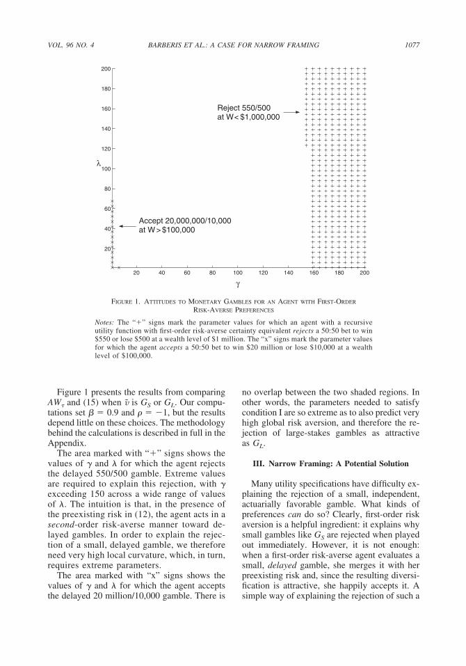
Figure 1 presents the results from comparingAW� and (15) when v is GS or GL. Our compu-tations set � � 0.9 and � � �1, but the resultsdepend little on these choices. The methodologybehind the calculations is described in full in theAppendix.

The area marked with “�” signs shows thevalues of � and for which the agent rejectsthe delayed 550/500 gamble. Extreme valuesare required to explain this rejection, with �exceeding 150 across a wide range of valuesof . The intuition is that, in the presence ofthe preexisting risk in (12), the agent acts in asecond-order risk-averse manner toward de-layed gambles. In order to explain the rejec-tion of a small, delayed gamble, we thereforeneed very high local curvature, which, in turn,requires extreme parameters.

The area marked with “x” signs shows thevalues of � and for which the agent acceptsthe delayed 20 million/10,000 gamble. There is

no overlap between the two shaded regions. Inother words, the parameters needed to satisfycondition I are so extreme as to also predict veryhigh global risk aversion, and therefore the re-jection of large-stakes gambles as attractiveas GL.

III. Narrow Framing: A Potential Solution

Many utility specifications have difficulty ex-plaining the rejection of a small, independent,actuarially favorable gamble. What kinds ofpreferences can do so? Clearly, first-order riskaversion is a helpful ingredient: it explains whysmall gambles like GS are rejected when playedout immediately. However, it is not enough:when a first-order risk-averse agent evaluates asmall, delayed gamble, she merges it with herpreexisting risk and, since the resulting diversi-fication is attractive, she happily accepts it. Asimple way of explaining the rejection of such a

FIGURE 1. ATTITUDES TO MONETARY GAMBLES FOR AN AGENT WITH FIRST-ORDER

RISK-AVERSE PREFERENCES

Notes: The “�” signs mark the parameter values for which an agent with a recursiveutility function with first-order risk-averse certainty equivalent rejects a 50:50 bet to win$550 or lose $500 at a wealth level of $1 million. The “x” signs mark the parameter valuesfor which the agent accepts a 50:50 bet to win $20 million or lose $10,000 at a wealthlevel of $100,000.


delayed gamble, then, is to suppose that theagent does not fully merge it with her preexist-ing risk, but that, to some extent, she evaluatesit in isolation. By “evaluates it in isolation,” wemean that the agent derives utility directly fromthe outcome of the gamble, and not just indi-rectly via its contribution to total wealth, as intraditional models. Equivalently, her utilityfunction depends on the outcome of the gambleover and above what that outcome implies fortotal wealth risk. This, is “narrow framing.”

We now check that preferences that allow forboth first-order risk aversion and narrow fram-ing can easily satisfy conditions I and II,whether the gambles are played out immedi-ately or with delay. A preference specificationthat incorporates both of these features has re-cently been developed by Barberis and Huang(2004). In their formulation, time t utility isgiven by

(16) Vt � W�Ct , �(Vt�1) b0Et��i

v� (Gi,t�1)��,where

(17) W�C, y� � ��1 � ��C� �y��1/�,

0 � � 1,

(18) ��V� � �E�V1 � ��1/�1 � ��,

0 � � 1,

(19) v� �x� � �x x for

x � 0x � 0 , � 1,

and where Gi,t�1 are specific gambles faced bythe agent whose uncertainty will be resolvedbetween time t and t � 1.

The term prefixed by b0 in (16) shows that,relative to the usual recursive specification in(1), utility can now depend on outcomes ofgambles Gi,t�1 over and above what those out-comes mean for total wealth risk: Gi,t�1 nowenters the utility function directly, and not justindirectly via time t � 1 utility, Vt�1. In otherwords, the specification in (16) allows for nar-row framing, with the parameter b0 controllingthe degree of narrow framing: a b0 of 0 meansno narrow framing at all, while a large b0 meansthat Gi,t�1 is evaluated almost completely in

isolation from other risks. First-order risk aver-sion is also introduced, this time through thepiecewise linearity of v� �. Since v� � exhibitsfirst-order risk aversion, there is no need for�� to do so; here, �� takes a simple powerutility form.

Barberis and Huang (2004) propose that anagent with these preferences evaluate an imme-diate gamble x at time � by, as before, insertingan infinitesimal time interval �� and applyingthe recursive calculation over this time step. Ifthe gamble is framed narrowly, the utility fromtaking it is

(20) W�0, ��V� � �� b0 E� �v� �x��

� W�0, ��J�W� � �� b0 E� �v� �x��

� W�0,��J�W� x�� b0E��v� �x��,

where J� is the time � � �� value function,while the utility from not taking it is

(21) W�0, ��V� � �� W�0, ��J�W� ��.

A delayed gamble at time � is evaluated, asbefore, by applying the recursive calculationover the time step from � to � � 1. If the gambleis framed narrowly, the utility from taking it is

(22) W�C�†, ��V� � 1 � b0 E� �v� �x��

� W�C�†, ��J�W� � 1 �� b0 E� �v� �x��

� W�C�†,��J��W� � C�

†�R� 1† x��

b0E� �v� �x��,

where J� is the time � � 1 value function, R��1†

is the return on invested wealth between � and� � 1, and where dagger signs denote optimalconsumption and portfolio choices; and the util-ity from not taking it is

(23) W�C*� , ��V� � 1 ��

� W�C*� , ��J��W� � C*� �R*� � 1 ��,

where optimal consumption and portfoliochoices are now denoted by asterisks. We con-trast C*� and R*��1 with C�

† and R��1† as a re-

minder that optimal consumption and portfoliochoices change when the gamble is accepted.


Using these expressions, we can check thatthe preferences in (16)–(19) can indeed satisfyconditions I and II, whether GS and GL areimmediate or delayed, so long as the gamblesare framed narrowly.11 To see the intuition,suppose that the 550/500 bet, whether immedi-ate or delayed, is framed narrowly, so that theagent thinks about it in isolation, to some extent.Since v�� is steeper for losses than for gains, thepotential loss of $500 looms larger than thepotential gain of $550, leading the agent toreject the gamble. In other words, if the agent’sfirst-order risk aversion is focused directly onthe 550/500 bet rather than just on her overallwealth risk, she will be reluctant to take the bet.

We consider the same environment as in theexample of Section IIA. We assume that, ini-tially, the agent’s only investment opportunityis a risky asset with gross return R between t andt � 1, where R has the distribution

(24) log R � N�0.04, 0.03�, i.i.d. over time.

Barberis and Huang (2004) show that, in thiscase, the agent’s time t value function takes theform

(25) J�Wt � � AWt

for all t, where the constant A is given by

(26) AWt � W�C*t , ��Vt � 1 ��

� W�C*t , ��J�Wt � 1 ��

� W�C*t ,��J��Wt � C*t �R��

� W�C*t ,A��Wt � C*t �R��.

For simplicity, we assume here that the agentdoes not frame her preexisting risk narrowly.

Now suppose that, at time �, the agent isoffered a gamble v, where v is either GS or GLand is either immediate or delayed. As before,the outcome of v does not affect, and is inde-pendent of, It and future economic uncertainty.As a result, whether the agent accepts v or not,her time t value function continues to be given

by equation (25) for t � � � �� in the case ofan immediate gamble, and for t � � � 1 in thecase of a delayed gamble. Expressions (20)–(23) then allow us to determine the agent’sattitudes to immediate and delayed versions ofGS and GL. The methodological details are de-scribed in full in the Appendix.

We set � and �, which have little directinfluence on attitudes to risk, to 0.9 and �1,respectively. Our calculations then show that,for a range of values of b0—including a b0 aslow as 0.001—it is easy to find parameter pairs(�, ) that satisfy conditions I and II, whetherthe gambles are immediate or delayed. For ex-ample, when b0 � 0.1, the pair (�, ) � (1.5, 3)can do so. The intuition is that a of 3 generatesenough sensitivity to losses to reject the 550/500 bet, with its 1.1 gain-to-loss ratio, when thatbet is evaluated to some extent in isolation; butit does not generate nearly enough sensitivity tolosses to reject the highly attractive 20 million/10,000 gamble.

IV. Application: Stock Market Participation

We have argued that a wide range of utilityfunctions, including even those with first-orderrisk aversion, have difficulty explaining anaversion to a small, independent, actuariallyfavorable gamble while also making sensiblepredictions about attitudes to large gambles.Utility functions that exhibit both first-orderrisk aversion and narrow framing offer a simpleway out of this difficulty.

We now show that our analysis has usefulimplications for financial markets, for example,for the stock market participation puzzle; the factthat, even though the stock market has a high meanreturn, many households have historically been re-luctant to allocate any money to it (Mankiw andZeldes, 1991; Haliassos and Bertaut, 1995).12

11 To satisfy conditions I and II, we only need the agentto frame GS narrowly. For the sake of treating the twogambles symmetrically, we suppose that the agent framesboth of them narrowly.

12 Mankiw and Zeldes (1991) report that, in 1984, only28 percent of households held any stock at all, and only 12percent held more than $10,000 in stock. Nonparticipationwas not simply the result of not having any liquid assets:even among households with more than $100,000 in liquidassets, only 48 percent held stock. Today, the fraction ofhouseholds that own stock is closer to 50 percent. Theparticipation puzzle is therefore primarily the puzzle ofwhy, historically, many people did not invest in equities,but also of why, today, people participate more. In thissection, we focus on the first part of the puzzle, and returnto the second part in Section V.


One approach to the participation puzzle in-vokes transaction costs of investing in thestock market; another examines whether non-stockholders have background risk that is cor-related with the stock market (John C. Heatonand Deborah J. Lucas, 1997, 2000; AnnetteVissing-Jorgensen, 2002). These approachesalmost certainly explain some of the observednonparticipation, but they may not be able toaccount for all of it. Polkovnichenko (2005)finds that, even among wealthy households, forwhom transaction costs are low, there is stillsubstantial nonparticipation; and StephanieCurcuru et al. (2005) question whether the cor-relation of the stock market with the back-ground risk of nonstockholders is high enoughto explain an equity allocation as low as zero.

Here, we investigate a third approach to theparticipation puzzle: a preference-based ap-proach. In particular, we try to understand whatkinds of preferences can generate nonparticipa-tion in the stock market for parameterizationsthat we would consider reasonable. We take areasonable parameterization to be one thatmakes sensible predictions about attitudes tolarge gambles; for example, one that satisfiescondition II, acceptance of the 20 million/10,000 gamble at wealth levels above $100,000.

It is already understood that preferences thatexhibit only second-order risk aversion havedifficulty addressing the participation puzzle(Heaton and Lucas, 1997, 2000). Our earlieranalysis suggests a more surprising prediction:that even preferences with first-order risk aver-sion will have trouble addressing this puzzle. Italso suggests that preferences that combinefirst-order risk aversion with narrow fram-ing—in this case, narrow framing of stock mar-ket risk—will have an easier time doing so.

To see the logic behind these predictions,note that, in the absence of narrow framing, anagent must evaluate stock market risk by merg-ing it with her preexisting risk and checking ifthe combination is attractive. For most house-holds, stock market risk has a correlation closeto zero with other important risks, such as laborincome risk, proprietary income risk, and houseprice risk (Heaton and Lucas, 2000). A smallequity position is therefore diversifying, and,according to our earlier analysis, the agent willfind this attractive, even if first-order riskaverse. Only an extreme parameterization of

her preferences will make her withdraw fromthe stock market entirely. Such a parameter-ization, however, almost always implies highglobal risk aversion, thereby violating condi-tion II.

A simple way out of this difficulty is tosuppose that, when the agent evaluates the stockmarket, she does not fully merge its risk withthe other risks she is already facing but, rather,thinks about it in isolation, to some extent. Byfocusing the agent’s first-order risk aversiondirectly on the stock market rather than just onher overall wealth risk, we can generate non-participation more easily.

In making these predictions, we are assumingthat our analysis of independent gambles is alsorelevant for gambles that are merely relativelyuncorrelated with other risks. While this islikely to be true, the only way to be sure is tocheck our predictions explicitly in a simpleportfolio choice setting. This is what we nowdo.

Consider an agent who, at the start of eachperiod, has a fixed fraction ��N of her wealth tiedup in a nonfinancial asset—our so-called pre-existing risk—with gross return

(27) log RN,t � 1 � gN �N�N,t � 1 ,

and who is wondering what fraction �S of herwealth to invest in the stock market, which hasgross return

(28) log RS,t � 1 � gS �S�S,t � 1 ,

where

(29) � �N,t

�S,t� � N��0

0� , � 1 �� 1�� ,

i.i.d. over time.

The remaining fraction of her wealth, 1 � ��N � �S,is invested in a risk-free asset earning a grossreturn of Rf, so that the return on total wealthbetween t and t � 1 is

(30) RW,t � 1 � �1 � �� N � �S �Rf

�� NRN,t � 1 �SRS,t � 1 .


In reality, of course, the fraction of an individ-ual’s wealth made up by a nonfinancial assetlike a house is likely to vary over time. Fixing itat ��N is a simplifying assumption, but is notcrucial for our results.

We solve this portfolio problem for threedifferent preference specifications: (a) as abenchmark, the power utility form

(31) E0 �t � 0

�

�tCt

1 � �

1 � �;

(b) recursive utility with first-order risk aversecertainty equivalent, or R-FORA, as in (1), (3),and (4); and (c), preferences that combine first-order risk aversion with narrow framing ofstock market risk, which, following the formu-lation in (16), can be written as

(32) Vt � W�Ct , ��Vt � 1� b0Et�v� �GS,t � 1��,

where GS,t�1, the stock market gamble theagent is taking, is given by

(33) GS,t � 1 � �S�Wt � Ct��RS,t � 1 � Rf�,

and where W( � , � ), ��, and v� � are given in(17)–(19).13

To match historical annual data, we set themean gS and volatility �S of log stock marketreturns to 0.06 and 0.2, respectively. We set themean gN and volatility �N of log returns on thenonfinancial asset to 0.04 and 0.03, respec-tively, and the fraction of nonfinancial wealth intotal wealth, ��N, to 0.75, but our results dependlittle on the values of these three parameters. Amore important parameter is �, the correlationof stock market risk with the agent’s preexistingrisk. Heaton and Lucas (2000) report correla-tions between stock market risk and three

major kinds of preexisting risk—labor in-come, proprietary income, and real estate— of�0.07, 0.14, and �0.2 in the aggregate, re-spectively. They also find that, in the crosssection of households, these correlationsrarely exceed 0.2, and, in their simulations,consider only correlations in the range [�0.1,0.2]. An � of 0.1 is therefore a reasonablebenchmark value. Finally, we set the grossrisk-free rate Rf to 1.02.

For these return process parameters, and foreach utility function in turn, we compute therange of preference parameters for which theagent allocates a fraction �S � 0 of overallwealth to the stock market, in other words, therange of parameters for which, even though thestock market offers a high mean rate of return,gS � 0.06, she still refuses to participate in it.(The solution technique used for preferencespecifications (b) and (c) is described in theAppendix.) We then check whether these pref-erence parameters are reasonable, in otherwords, whether they are consistent with condi-tion II. Specifically, we check whether an agentwith wealth of $100,000, a fraction ��N of whichis invested in the nonfinancial asset with returndistribution in (27), and a fraction 1 � ��N ofwhich is invested in the risk-free asset, wouldaccept a 20 million/10,000 gamble. As in Sec-tions IIA and III, we use � � 0.9, � � �1, andb0 � 0.1.

Power utility preferences illustrate the basicpuzzle. For the return process parameters above,� � 137 is required for a �S � 0 allocation tothe stock market; but for such �, the agent isvery risk averse, and would turn down a 20million/10,000 gamble at a wealth level of$100,000, violating condition II.

Figures 2 and 3 present results for prefer-ences (b) and (c), respectively. In each figure,the “�” signs indicate the parameters for whichthe agent chooses a �S � 0 allocation to thestock market, while the “x” signs show theparameters for which she accepts GL.

Figure 2 confirms that, for R-FORA pref-erences, with first-order risk aversion but nonarrow framing, it is hard to generate nonpar-ticipation for reasonable parameter values. Infact, for this implementation of first-order riskaversion, it is impossible: there is no overlapbetween the two shaded regions. In the ab-sence of narrow framing, a positive position

13 The simplest way to define the stock market gamble is�S(Wt � Ct)(RS,t�1 � 1): the capital allocated to the stockmarket multiplied by the net return on the stock market. Fortractability, we adopt the slight modification of defining thegain or loss on the stock market gamble relative to therisk-free rate Rf. The interpretation is that a stock marketreturn is only considered a gain, and only delivers positiveutility, if it is higher than the return on T-Bills.


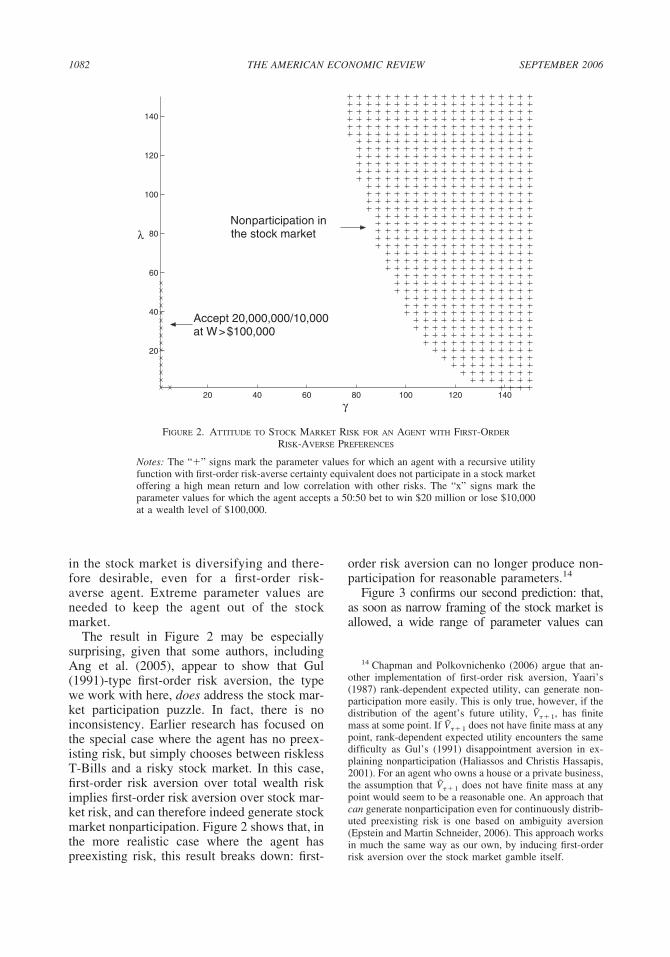
in the stock market is diversifying and there-fore desirable, even for a first-order risk-averse agent. Extreme parameter values areneeded to keep the agent out of the stockmarket.

The result in Figure 2 may be especiallysurprising, given that some authors, includingAng et al. (2005), appear to show that Gul(1991)-type first-order risk aversion, the typewe work with here, does address the stock mar-ket participation puzzle. In fact, there is noinconsistency. Earlier research has focused onthe special case where the agent has no preex-isting risk, but simply chooses between risklessT-Bills and a risky stock market. In this case,first-order risk aversion over total wealth riskimplies first-order risk aversion over stock mar-ket risk, and can therefore indeed generate stockmarket nonparticipation. Figure 2 shows that, inthe more realistic case where the agent haspreexisting risk, this result breaks down: first-

order risk aversion can no longer produce non-participation for reasonable parameters.14

Figure 3 confirms our second prediction: that,as soon as narrow framing of the stock market isallowed, a wide range of parameter values can

14 Chapman and Polkovnichenko (2006) argue that an-other implementation of first-order risk aversion, Yaari’s(1987) rank-dependent expected utility, can generate non-participation more easily. This is only true, however, if thedistribution of the agent’s future utility, V��1, has finitemass at some point. If V��1 does not have finite mass at anypoint, rank-dependent expected utility encounters the samedifficulty as Gul’s (1991) disappointment aversion in ex-plaining nonparticipation (Haliassos and Christis Hassapis,2001). For an agent who owns a house or a private business,the assumption that V��1 does not have finite mass at anypoint would seem to be a reasonable one. An approach thatcan generate nonparticipation even for continuously distrib-uted preexisting risk is one based on ambiguity aversion(Epstein and Martin Schneider, 2006). This approach worksin much the same way as our own, by inducing first-orderrisk aversion over the stock market gamble itself.

FIGURE 2. ATTITUDE TO STOCK MARKET RISK FOR AN AGENT WITH FIRST-ORDER

RISK-AVERSE PREFERENCES

Notes: The “�” signs mark the parameter values for which an agent with a recursive utilityfunction with first-order risk-averse certainty equivalent does not participate in a stock marketoffering a high mean return and low correlation with other risks. The “x” signs mark theparameter values for which the agent accepts a 50:50 bet to win $20 million or lose $10,000at a wealth level of $100,000.


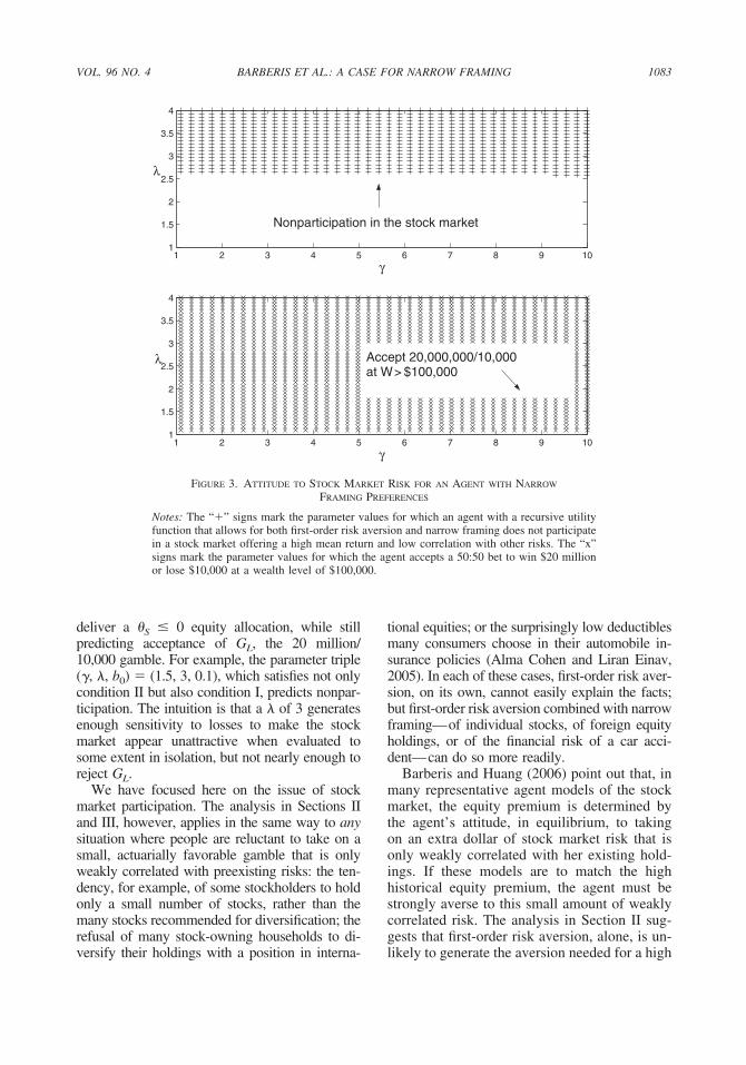
deliver a �S � 0 equity allocation, while stillpredicting acceptance of GL, the 20 million/10,000 gamble. For example, the parameter triple(�, , b0) � (1.5, 3, 0.1), which satisfies not onlycondition II but also condition I, predicts nonpar-ticipation. The intuition is that a of 3 generatesenough sensitivity to losses to make the stockmarket appear unattractive when evaluated tosome extent in isolation, but not nearly enough toreject GL.

We have focused here on the issue of stockmarket participation. The analysis in Sections IIand III, however, applies in the same way to anysituation where people are reluctant to take on asmall, actuarially favorable gamble that is onlyweakly correlated with preexisting risks: the ten-dency, for example, of some stockholders to holdonly a small number of stocks, rather than themany stocks recommended for diversification; therefusal of many stock-owning households to di-versify their holdings with a position in interna-

tional equities; or the surprisingly low deductiblesmany consumers choose in their automobile in-surance policies (Alma Cohen and Liran Einav,2005). In each of these cases, first-order risk aver-sion, on its own, cannot easily explain the facts;but first-order risk aversion combined with narrowframing—of individual stocks, of foreign equityholdings, or of the financial risk of a car acci-dent—can do so more readily.

Barberis and Huang (2006) point out that, inmany representative agent models of the stockmarket, the equity premium is determined bythe agent’s attitude, in equilibrium, to takingon an extra dollar of stock market risk that isonly weakly correlated with her existing hold-ings. If these models are to match the highhistorical equity premium, the agent must bestrongly averse to this small amount of weaklycorrelated risk. The analysis in Section II sug-gests that first-order risk aversion, alone, is un-likely to generate the aversion needed for a high

FIGURE 3. ATTITUDE TO STOCK MARKET RISK FOR AN AGENT WITH NARROW

FRAMING PREFERENCES

Notes: The “�” signs mark the parameter values for which an agent with a recursive utilityfunction that allows for both first-order risk aversion and narrow framing does not participatein a stock market offering a high mean return and low correlation with other risks. The “x”signs mark the parameter values for which the agent accepts a 50:50 bet to win $20 millionor lose $10,000 at a wealth level of $100,000.


premium, a prediction confirmed by Epstein andZin (2001) and Barberis and Huang (2006). Theanalysis in Section III, however, suggests that acombination of first-order risk aversion and nar-row framing—here, narrow framing of stockmarket risk—will more easily generate the re-quired aversion, and hence also, a high pre-mium. Shlomo Benartzi and Thaler (1995) andBarberis et al. (2001) confirm that models basedon loss aversion over narrowly framed stockmarket risk can indeed generate sizeable equitypremia.

V. Interpreting Narrow Framing

We have argued that preferences that com-bine first-order risk aversion with narrow fram-ing may be helpful for understanding attitudesto both independent monetary gambles and thestock market. Of the two features, narrow fram-ing is the more unusual. We therefore end bydiscussing its interpretation in more detail.

One way narrow framing can arise is if anagent takes nonconsumption utility, such as re-gret, into account. Regret is the pain we feelwhen we realize that we would be better offtoday if we had taken a different action in thepast. Even if a gamble that the agent accepts isjust one of many risks that she faces, it is stilllinked to a specific decision, namely the deci-sion to accept the gamble. As a result, it exposesthe agent to possible future regret: if the gambleturns out badly, the agent may regret the deci-sion to accept it. Consideration of nonconsump-tion utility therefore leads quite naturally topreferences that depend on the outcomes ofgambles over and above what those outcomesmean for total wealth.

Another view of narrow framing is proposedby Kahneman (2003). He suggests that it ariseswhen decisions are made intuitively, rather thanthrough effortful reasoning. Since intuitivethoughts are by nature spontaneous, they areheavily shaped by the features of the situation athand that come to mind most easily—to use thetechnical term, by the features that are most“accessible.” When an agent is offered a 50:50bet to win $550 or lose $500, the outcomes ofthe gamble, $550 and $500, are instantly acces-sible; much less accessible, however, is the dis-tribution of future outcomes the agent facesafter integrating the 550/500 bet with all of herother risks. As a result, if the agent thinks about

the gamble intuitively, the distribution of thegamble, taken alone, may play a more importantrole in decision-making than would be pre-dicted by traditional utility functions definedonly over wealth or consumption.

By providing the outline of a theory of fram-ing, Kahneman (2003) makes framing a moretestable concept than it was before. Thaler et al.(1997) illustrate the kind of test one can do. Inan experimental setting, they ask subjects howthey would allocate between a risk-free assetand a risky asset over a long time horizon, suchas 30 years. The key manipulation is that somesubjects are shown draws from the distributionof short-term asset returns—the distribution ofmonthly returns, say—while others are showndraws from a long-term return distribution—thedistribution of 30-year returns, say. Since theyhave the same decision problem, the two groupsof subjects should make similar allocation de-cisions: subjects who see short-term returnsshould simply use them to infer the more rele-vant long-term returns. If this requires too mucheffort, however, Kahneman’s (2003) frameworksuggests that these subjects will instead use thereturns that are most accessible to them, namelythe short-term returns they were shown. Sincelosses occur more often in high-frequency data,they will perceive the risky asset to be espe-cially risky and will allocate less to it. This isexactly Thaler et al.’s (1997) finding.

In Section IV, we addressed the stock marketparticipation puzzle by saying that agents mayget utility from the outcome of their stock mar-ket investments over and above what that out-come means for their overall wealth; in otherwords, they may frame the stock market nar-rowly. Is this a plausible hypothesis?

It seems to us that both the “regret” and“accessibility” interpretations of narrow fram-ing could indeed apply to decisions about thestock market. Allocating some fraction of herwealth to the stock market constitutes a concreteaction on the part of the agent—one that shemay later regret if her stock market gambleturns out poorly.15

15 Of course, investing in T-Bills may also lead to regretif the stock market goes up in the meantime. Regret isthought to be stronger, however, when it stems from havingtaken an action—for example, moving one’s savings fromthe default option of a riskless bank account to the stockmarket—than from not having taken an action—for exam-


Alternatively, given our daily exposure, fromnewspapers, books, and other media, to infor-mation about the distribution of stock marketrisk, such information is very accessible. Muchless accessible is any information as to the dis-tribution of future outcomes once stock marketrisk is merged with the other kinds of risk thatpeople often face. Applying Kahneman’s (2003)framework, judgments about how much to investin the stock market might therefore be made, tosome extent, using a narrow frame. Over time, ofcourse, people may learn that their intuitive deci-sion-making is leading them astray, and mayswitch to the normatively superior strategy of par-ticipating in the stock market. This may be onefactor behind the rise in stock market participationover the past 15 years.

The so-called “disposition effect”—the ten-dency of individual investors to sell stocks intheir portfolios that have risen in value sincepurchase, rather than fallen—suggests thatpeople may not only frame overall stock mar-ket risk narrowly, but individual stock riskas well: perhaps the simplest way of explain-ing the disposition effect is to posit thatpeople receive direct utility from realizing again or loss on an individual stock thatthey own.16

Alok Kumar and Sonya S. Lim (2005) il-lustrate another approach to testing framing-based theories. They point out that, under thehypothesis that the disposition effect is due tonarrow framing, people who are more suscep-tible to narrow framing will display the dis-

position effect more. They identify thesemore susceptible traders as those who tend toexecute just one trade, as opposed to severaltrades, on any given day: if a trader executesjust one trade on a given day, the gain or lossfor that trade will be more accessible, makingnarrow framing more likely. The data confirmthe prediction: the “one-trade-a-day” tradersexhibit the disposition effect more.

VI. Conclusion

We argue that narrow framing, whereby anagent who is offered a new gamble evaluatesthat gamble in isolation, separately from otherrisks she already faces, may be a more impor-tant feature of decision-making than previouslyrealized. Our starting point is the evidence thatpeople are often averse to a small, independentgamble, even when the gamble is actuariallyfavorable. We find that a surprisingly widerange of utility functions, including many non-expected utility specifications, have trouble ex-plaining this evidence; but that this difficultycan be overcome by allowing for narrow fram-ing. Our analysis makes predictions as to whatkinds of preferences can most easily address thestock market participation puzzle, as well asother related financial puzzles. We confirmthese predictions in a simple portfolio choicesetting.

Our analysis does not prove that narrow fram-ing is at work in the case of monetary gambles,nor that it is at work in the case of stock marketnonparticipation. Given the difficulties faced bystandard preferences, however, the narrow fram-ing view may need to be taken more seriouslythan before. With the emergence of new theoriesof framing, such as that of Kahneman (2003), weexpect to see new tests of framing-based hypoth-eses. Such tests should, in time, help us learn moreabout the role that narrow framing plays in indi-vidual decision-making.

APPENDIX

PROOF OF PROPOSITION 1:We prove the proposition for a certainty equivalent functional �� more general than (4), namely

(34) u��V�� E�u�V�� 1�E��u�V� � u��V��1�V � ��V��, � 1,

where u� has a positive first derivative and a negative second derivative. For

ple, leaving one’s savings in place at the bank. In short,errors of commission are more painful than errors of omis-sion (Kahneman and Tversky, 1982).

16 Terrance Odean (1998) argues that other potentialexplanations of the disposition effect—explanations basedon informed trading, taxes, rebalancing, or transactioncosts—fail to capture important features of the data.


(35) u�x� �x1 � �

1 � �, 0 � � 1,

this reduces to (4).Note first that, since V��1 does not have finite mass at �(V��1), a small change in the period � � 1

value function, �V��1 � �V(W��1, I��1), changes the certainty equivalent by

(36) �� E�u�V� � 1��V� � 1� � � 1�E�u�V� � 1�1�V� � 1 � ��V� � 1�

u��1 � � 1�Prob�V� � 1 � �� o��V� � 1��,

where � denotes �(V��1), �x� � E(�x�), and limx30(o(x)/x) � 0, by definition.Denote the gamble k� described in the proposition by v. Assume, for now, that the agent does not

optimally adjust her time � consumption and portfolio choice if she takes the gamble. Then,

(37) �V� � 1 � JW �W� � 1 , I� � 1 �v o��v��,

which, from (36), implies

(38) �� E�u�V��1�JW�W��1, I��1�v� � � 1�E�u�V��1�1�V��1 � ��JW�W��1, I��1�v�

u��1 � � 1�Prob�V� � 1 � �� o��v��.

Since v is independent of other economic uncertainty, we have

(39) �� E�v�E�u�V��1�JW�W��1, I��1�� 1�E�u�V��1�1�V��1 � ��JW�W��1, I��1��

u��1 � � 1�Prob�V� � 1 � �� o��v��,

so that, to first order, the certainty equivalent of V��1 depends only on the expected value of thegamble v, not on its standard deviation.

To complete the proof, note that the aggregator function W( � , � ) does not generate any first-orderdependence on the standard deviation of v. In addition, assuming that the agent adjusts her time �consumption and portfolio choice optimally when accepting v introduces only terms of the secondorder of v. The agent is therefore second-order risk averse over v.

COMPUTING ATTITUDES TO MONETARY GAMBLES

Recursive Utility with First-Order Risk Averse Certainty Equivalent

We now describe the methodology behind the delayed gamble calculations of Section IIA. Animportant parameter is the constant A in (13). From (14), A satisfies

(40) AWt � maxCt

W�Ct , A��Wt � Ct�R�� maxCt

�1 � ��Ct� ��Wt � Ct�

�A��R��1/�

� max�

Wt�1 � �� 1 � ��A��R��1/�,

where � is the fraction of wealth consumed at time t. The first-order condition is

(41) �1 � �� 1 � ��1 � �� 1A��,

where � � �(R). When substituted into (40), this gives


(42) A � �1 � ��1/�� 1�/�.

Substituting this into (41) leads to

(43) � � 1 � �1/�1 � ��/�1 � ��.

Therefore, given �, which can be computed from its definition in (4), we obtain � from (43) and Afrom (42).

If the agent does not take the delayed gamble v, her utility at time � is AW�. If she does take v,her utility, from (15), is

(44) maxC�

W�C� , A��W� � C��R v��

� max�

W� �(1 � �)�� (1 � �)�A��R v

W�(1 � �)��1/�

� AW� ,

where A was computed above. This maximization can be performed numerically. We can thencompare A to A to see if the agent should take the delayed gamble.

Recursive Utility with Both First-Order Risk Aversion and Narrow Framing

We now describe the methodology behind the gamble calculations of Section III. An importantparameter is the constant A in (25). From (26), A satisfies

(45) AWt � maxCt

W�Ct , A��Wt � Ct�R�� maxCt

�1 � ��Ct� ��Wt � Ct�

�A�E�R1��/�1��1/�

� max�

Wt�1 � �� 1 � ��A�E�R1��/�1��1/�,

where � is the fraction of wealth consumed at time t. The first-order condition is

(46) �1 � �� 1 � ��1 � �� 1 A��E�R1 � ��/�1 � ��,

which, when substituted into (45), gives

(47) A � �1 � ��1/�� 1�/�.

Substituting this into (46) leads to

(48) � � 1 � �1/�1 � ��E�R1 � ��/��1 � ��1 � ��.

Therefore, we obtain � from (48) and A from (47).From (20) and (21), the agent takes an immediate gamble x if and only if

(49) A�E�W� x�1 � � 1/�1 � �� b0 E� �v� �x�� AW� ,

where A was computed above.We now turn to the case of delayed gambles. From (23), if the agent does not take a delayed

gamble x, her utility is AW�, where A was computed above. If she takes the delayed gamble, herutility, from (22), is


(50) maxC�

W�C� , A��W� � C��R x� b0E��v� �x��

� max�

W� �(1 � �)�� (1 � �)� A�E�R x

W�(1 � �)�1��1/(1��)

� b0E��v� � x

W�(1 � �)��1/�

� AW� ,

where A was computed above. This maximization can be performed numerically. We can thencompare A to A to see if the agent should take the delayed gamble.

PORTFOLIO CHOICE CALCULATIONS

We now describe the methodology behind the portfolio choice calculations of Section IV.

Recursive Utility with First-Order Risk Averse Certainty Equivalent

Epstein and Zin (1989) show that, in the i.i.d. setting of Section IV, the consumption-wealth ratiois a constant �, the fraction of wealth allocated to the stock market is a constant �S, and the time tvalue function is J(Wt) � AWt for all t. The agent’s problem becomes

(51) maxCt ,�S

W�Ct , ��Vt � 1�� maxCt ,�S

W�Ct , A��Wt � 1��

� max�,�S

Wt��1 � �� 1 � ��A��RW,t � 1�� 1/�,

where RW,t�1 is defined in (30). The consumption and portfolio problems are therefore separable.The portfolio problem is

(52) max�S

��RW,t � 1�,

which, given the definition of �� in (4), can be solved in a straightforward fashion.

Recursive Utility with Both First-Order Risk Aversion and Narrow Framing

Barberis and Huang (2004) show that, in the i.i.d. setting of Section IV, the consumption-wealthratio is a constant �, the fraction of wealth allocated to the stock market is a constant �S, and the timet value function is J(Wt) � AWt for all t. The agent’s problem becomes

(53) AWt � maxCt ,�S

W�Ct , ��Vt � 1� b0Et�v� �GS,t � 1�� maxCt ,�S

W�Ct , A��Wt�1� b0Et�v� �GS,t�1��

� max�

Wt��1 � �� 1 � ��B*�� 1/�,

where GS,t�1 is defined in (33) and

(54) B* � max�S

A�E�RW,t � 11 � � � 1/�1 � �� b0�SEt�v� �RS,t � 1 � Rf��.


The only difficulty with the portfolio problem in (54) is that it depends on the value functionconstant A. To handle this, note that the first-order condition for consumption in (53) is

(55) �1 � �� 1 � ��1 � �� 1�B*��.

Substituting this into (53) gives

(56) A � �1 � ��1/�� 1�/�.

The problem can now be solved as follows. Guess a candidate value of �, substitute it into (56) togenerate a candidate A, and then solve portfolio problem (54) for that A. Take the B* that results anduse equation (55) to generate a new �. Continue this iteration until convergence occurs. Theconverged values represent an optimum.

REFERENCES

Abdellaoui, Mohammed; Bleichrodt, Han andParaschiv, Corina. “Loss Aversion underProspect Theory: A Parameter-Free Measure-ment.” Unpublished Paper, 2005.

Ang, Andrew; Bekaert, Geert and Liu, Jun. “WhyStocks May Disappoint.” Journal of Finan-cial Economics, 2005, 76(3), pp. 471–508.

Barberis, Nicholas and Huang, Ming. “Prefer-ences with Frames: A New Utility Specifica-tion That Allows for the Framing of Risks.”Unpublished Paper, 2004.

Barberis, Nicholas and Huang, Ming. “The LossAversion/Narrow Framing Approach to theEquity Premium Puzzle,” in Rajnish Mehra,ed., Handbook of investments: Equity pre-mium. Amsterdam: Elsevier Science, North-Holland, 2006.

Barberis, Nicholas; Huang, Ming and Santos,Tano. “Prospect Theory and Asset Prices.”Quarterly Journal of Economics, 2001,116(1), pp. 1–53.

Barberis, Nicholas; Huang, Ming and Thaler,Richard H. “Individual Preferences, Mone-tary Gambles and the Equity Premium.” Na-tional Bureau of Economic Research, Inc.,NBER Working Papers: No. 9997, 2003.

Benartzi, Shlomo and Thaler, Richard H. “Myo-pic Loss Aversion and the Equity PremiumPuzzle.” Quarterly Journal of Economics,110(1), pp. 73–92.

Chapman, David A. and Polkovnichenko, Valery.“Heterogeneity in Preferences and Asset Mar-ket Outcomes.” Unpublished Paper, 2006.

Chetty, Raj. “Consumption Commitments, Un-employment Durations, and Local Risk

Aversion.” National Bureau of EconomicResearch, Inc., NBER Working Papers: No.10211, 2004.

Cohen, Alma and Einav, Liran. “Estimating RiskPreferences from Deductible Choice.” Na-tional Bureau of Economic Research, Inc.,NBER Working Papers: No. 11461, 2005.

Curcuru, Stephanie; Heaton, John C.; Lucas,Deborah J. and Moore, Damien. “Heteroge-neity and Portfolio Choice: Theory and Evi-dence,” in Yacine Ait-Sahalia and Lars PeterHansen, eds., Handbook of financial economet-rics. Amsterdam: Elsevier Science, North-Holland, 2005.

Epstein, Larry G. and Schneider, Martin. “Learn-ing under Ambiguity.” Unpublished Paper,2006.

Epstein, Larry G. and Zin, Stanley E. “Substitu-tion, Risk Aversion, and the Temporal Be-havior of Consumption and Asset Returns: ATheoretical Framework.” Econometrica, 1989,57(4), pp. 937–69.

Epstein, Larry G. and Zin, Stanley E. “ ‘First-Order’ Risk Aversion and the Equity PremiumPuzzle.” Journal of Monetary Economics,1990, 26(3), pp. 387–407.

Epstein, Larry G. and Zin, Stanley E. “The Inde-pendence Axiom and Asset Returns.” Jour-nal of Empirical Finance, 2001, 8(5), pp.537–72.

Gul, Faruk. “A Theory of Disappointment Aver-sion.” Econometrica, 1991, 59(3), pp. 667–86.

Haliassos, Michael and Bertaut, Carol C. “WhyDo So Few Hold Stocks?” Economic Jour-nal, 1995, 105(432), pp. 1110–29.

Heaton, John C. and Lucas, Deborah J. “MarketFrictions, Savings Behavior, and Portfolio


Choice.” Macroeconomic Dynamics, 1997,1(1), pp. 76–101.

Heaton, John C. and Lucas, Deborah J. “PortfolioChoice in the Presence of Background Risk.”Economic Journal, 2000, 110(460), pp. 1–26.

Kahneman, Daniel. “Maps of Bounded Rational-ity: Psychology for Behavioral Economics.”American Economic Review, 2003, 93(5), pp.1449–75.

Kahneman, Daniel and Lovallo, Dan. “TimidChoices and Bold Forecasts: A CognitivePerspective on Risk Taking.” ManagementScience, 1993, 39(1), pp. 17–31.

Kahneman, Daniel and Tversky, Amos. “ThePsychology of Preferences.” Scientific Amer-ican, 1982, 246(1), pp. 160–73.

Kumar, Alok and Lim, Sonya S. “How Do Deci-sion Frames Influence the Stock InvestmentChoices of Individual Investors?” Unpub-lished Paper, 2005.

Mankiw, N. Gregory and Zeldes, Stephen P. “TheConsumption of Stockholders and Nonstock-holders.” Journal of Financial Economics,1991, 29(1), pp. 97–112.

Odean, Terrance. “Are Investors Reluctant toRealize Their Losses?” Journal of Finance,1998, 53(5), pp. 1775–98.

Polkovnichenko, Valery. “Household PortfolioDiversification: A Case for Rank-DependentPreferences.” Review of Financial Studies,2005, 18(4), pp. 1467–1502.

Rabin, Matthew. “Risk Aversion and Expected-Utility Theory: A Calibration Theorem.”Econometrica, 2000, 68(5), pp. 1281–92.

Rabin, Matthew and Thaler, Richard H. “Anom-

alies: Risk Aversion.” Journal of EconomicPerspectives, 2001, 15(1), pp. 219–32.

Read, Daniel; Loewenstein, George and Rabin,Matthew. “Choice Bracketing.” Journal ofRisk and Uncertainty, 1999, 19(1–3), pp.171–97.

Redelmeier, Donald A. and Tversky, Amos. “Onthe Framing of Multiple Prospects.” Psycho-logical Science, 1992, 3(3), pp. 191–93.

Segal, Uzi and Spivak, Avia. “First Order versusSecond Order Risk Aversion.” Journal ofEconomic Theory, 1990, 51(1), pp. 111–25.

Thaler, Richard H.; Tversky, Amos; Kahneman,Daniel and Schwartz, Alan. “The Effect ofMyopia and Loss Aversion on Risk Taking:An Experimental Test.” Quarterly Journal ofEconomics, 1997, 112(2), pp. 647–61.

Tversky, Amos and Kahneman, Daniel. “TheFraming of Decisions and the Psychology ofChoice.” Science, 1981, 211(4481), pp. 453–58.

Tversky, Amos and Kahneman, Daniel. “Ad-vances in Prospect Theory: CumulativeRepresentation of Uncertainty.” Journal ofRisk and Uncertainty, 1992, 5(4), pp. 297–323.

Vissing-Jorgensen, Annette. “Towards an Expla-nation of Household Portfolio Choice Hetero-geneity: Nonfinancial Income and ParticipationCost Structures.” National Bureau of EconomicResearch, Inc., NBER Working Papers: No.8884, 2002.

Yaari, Menahem E. “The Dual Theory of Choiceunder Risk.” Econometrica, 1987, 55(1), pp.95–115.


individual preferences, monetary gambles, and stock market...

Documents