inducing environmental disclosures: a dynamic …psun/bio/inspection.pdf · our analysis further...

This article was downloaded by: [152.3.34.72] On: 17 May 2016, At: 09:35Publisher: Institute for Operations Research and the Management Sciences (INFORMS)INFORMS is located in Maryland, USA

Operations Research

Publication details, including instructions for authors and subscription information:http://pubsonline.informs.org

Inducing Environmental Disclosures: A DynamicMechanism Design ApproachShouqiang Wang, Peng Sun, Francis de Véricourt

To cite this article:Shouqiang Wang, Peng Sun, Francis de Véricourt (2016) Inducing Environmental Disclosures: A Dynamic Mechanism DesignApproach. Operations Research 64(2):371-389. http://dx.doi.org/10.1287/opre.2016.1476

Full terms and conditions of use: http://pubsonline.informs.org/page/terms-and-conditions

This article may be used only for the purposes of research, teaching, and/or private study. Commercial useor systematic downloading (by robots or other automatic processes) is prohibited without explicit Publisherapproval, unless otherwise noted. For more information, contact [email protected].

The Publisher does not warrant or guarantee the article’s accuracy, completeness, merchantability, fitnessfor a particular purpose, or non-infringement. Descriptions of, or references to, products or publications, orinclusion of an advertisement in this article, neither constitutes nor implies a guarantee, endorsement, orsupport of claims made of that product, publication, or service.

Copyright © 2016, INFORMS

Please scroll down for article—it is on subsequent pages

INFORMS is the largest professional society in the world for professionals in the fields of operations research, managementscience, and analytics.For more information on INFORMS, its publications, membership, or meetings visit http://www.informs.org

http://pubsonline.informs.org

http://dx.doi.org/10.1287/opre.2016.1476

http://pubsonline.informs.org/page/terms-and-conditions

http://www.informs.org

OPERATIONS RESEARCHVol. 64, No. 2, March–April 2016, pp. 371–389ISSN 0030-364X (print) � ISSN 1526-5463 (online) http://dx.doi.org/10.1287/opre.2016.1476

© 2016 INFORMS

Inducing Environmental Disclosures: A DynamicMechanism Design Approach

Shouqiang WangNaveen Jindal School of Management, The University of Texas at Dallas, Richardson, Texas 75080, [email protected]

Peng SunFuqua School of Business, Duke University, Durham, North Carolina 27708, [email protected]

Francis de VéricourtESMT European School of Management and Technology, 10178 Berlin, Germany, [email protected]

This paper studies the design of voluntary disclosure regulations for a firm that faces a stochastic environmental hazard. Theoccurrence of such a hazard is known only to the firm. The regulator, if finding a hazard, collects a fine and mandates thefirm to perform costly remediation that reduces the environmental damage. The regulator may inspect the firm at any time touncover the hazard. However, because inspections are costly, the regulator also offers a reward to the firm for voluntarilydisclosing the hazard. The reward corresponds to either a subsidy or a reduced fine, depending on whether it is positive ornegative. Thus, the regulator needs to dynamically determine the reward and inspection policy that minimizes expectedsocietal cost in the long run. We model this problem as a dynamic adverse selection problem with costly state verification incontinuous time. Despite the complexity and generality of this setup, we show that the optimal regulation policy follows avery simple cyclic structure, which we fully characterize in closed form. Specifically, the regulator runs scheduled inspectionsperiodically. After each inspection, the reward level decreases over time until a subsequent inspection takes place. If a hazardis not revealed, the reward level is reset to a high level, restarting the cycle. In contrast to the reward level, the mandatedremediation level is constant over time. Nonetheless, when subsidies are not allowed in the industry, we show that theregulator should dynamically adjust this remediation level, which then acts as a substitute for a subsidy. Our analysis furtherreveals that optimal inspection frequency increases not only when the inspection accuracy decreases, but also when the penaltyfor not disclosing the hazard increases.

Keywords: dynamic mechanism design; optimal control; asymmetric information; environmental regulation; voluntarydisclosure.

Subject classifications : dynamic programming/optimal control; games/group/decisions; environment.Area of review : Operations and Supply Chains.History : Received June 2014; revisions received January 2015, September 2015; accepted December 2015. Published online

in Articles in Advance February 29, 2016.

1. IntroductionEnvironmental inspections (also called audits) are indispens-able regulatory instruments used to expose environmentalnoncompliance in private industries (Cohen 1999). However,inspections are costly and sometimes ineffective, especiallywhen hazards result from random events beyond firms’control, such as equipment malfunctions or natural causes(Beavis and Walker 1983, Kim 2015). To improve the effi-cacy of their investigative tools and to limit the use ofinspections, regulatory agencies have instituted voluntary dis-closure programs, which reward companies for self-reportingenvironmental hazards. The Audit Policy of the U.S. Envi-ronmental Protection Agency (EPA), for instance, eliminatesor significantly reduces penalties for firms that self-reporthazards (EPA 2000).

Nonetheless, designing an efficient and effective disclosureprogram remains a challenging task, as evidenced by thefailure of previous voluntary programs. For instance, the

EPA had to terminate one of its key initiatives (Shiffmanet al. 2009); see also Rivera et al. (2006) or King andLenox (2000). Indeed, although the notion that incentives forself-reporting can serve as cheaper substitutes for inspectionsmay be well established (Kaplow and Shavell 1994, Malik1993), how to efficiently operationalize this principle remainspoorly understood.

The purpose of this paper, therefore, is to provide theoret-ical guidelines for designing efficient voluntary disclosureprograms that combine reward and inspection instrumentsto detect an environmental hazard that occurs randomlybeyond the firm’s control. The regulator is not immediatelyaware of such a hazard, and the firm can choose to concealit to evade or delay costly regulatory consequences. Thiscorresponds, for instance, to the leakage of a toxic substance.Because of the nature of this setting in which information ishidden (i.e., adverse selection), we formulate the problemof setting reward levels for self-reporting over time usinga dynamic mechanism design framework. We incorporate

371

Dow

nloa

ded

from

info

rms.

org

by [

152.

3.34

.72]

on

17 M

ay 2

016,

at 0

9:35

. Fo

r pe

rson

al u

se o

nly,

all

righ

ts r

eser

ved.

mailto:[email protected]



Wang, Sun, and de Véricourt: Inducing Environmental Disclosures: A Dynamic Mechanism Design Approach372 Operations Research 64(2), pp. 371–389, © 2016 INFORMS

inspection instruments by enriching the model with costlystate verifications.

The main contribution of this paper is to demonstratethat, despite the complex strategic and dynamic interactionsbetween the regulator and the firm, and the generality of theregulation policies under consideration, the optimal policytakes on a simple cyclic structure. The policy is characterizedin closed form and is easy to compute and implement.

Specifically, we consider a regulator who seeks to discoverwhether a random environmental hazard has occurred ata firm. If a hazard that imposes adverse consequences onsociety is found, the regulator mandates that the firm incursa remediation (or repair) cost to remove the hazard andpays compensations for environmental damages. These costs,however, encourages the firm to conceal the hazard. Thefirm’s incentives, therefore, are not aligned with those of theregulator.

To determine whether a hazard has occurred, the regulatorcan decide at any time (possibly randomly) to inspect thefirm and inflict a nondisclosure penalty if a hazard is detected.Inspections, however, are costly and may be imperfect.

To limit the use of inspections, the regulator can providethe firm with incentives for voluntarily disclosing the hazard,in the form of a monetary reward or an adjusted remediationlevel. The reward corresponds to either a subsidy or areduced fine, depending on whether the reward amount ispositive or negative. Varying this amount according to thetime the hazard is disclosed adjusts the firm’s incentiveon when to report the hazard. Similarly, the regulator canalso adjust the level of mandated remediation levels and theassociated costs over time.

The regulator’s objective is to minimize expected societalcost in the long run, that is, to maximize social welfare.Following the regulation economics literature, the rewardfor voluntary disclosure generates frictions to the economyin the form of a shadow cost of public funds incurred bythe regulator (Laffont and Tirole 1993, Assumption 8 onpage 38). That is, each dollar spent by the regulator is raisedthrough distortionary taxes, which are costly to society.

In the presence of these frictions, and when inspectionsare perfect (i.e., inspections always reveal an existing hazard),we show that the optimal policy has a simple deterministiccyclic structure. The regulator starts the cycle by offering areward and mandates a remediation level when the hazardis self-reported. The reward amount decreases over timethroughout the cycle, until an inspection takes place. If thatinspection does not reveal a hazard, the reward amount isreset to its initial level, restarting the cycle. The mandatedremediation level, by contrast, remains constant over time.Such an optimal policy proceeds as long as no hazard isrevealed through disclosure or inspection. (Figures 3 and 4in §5 visualize this optimal policy.)

When inspections are imperfect (i.e., the probability offinding a hazard is less than one), the optimal policy followsa similar cyclic structure, but differs in two aspects (Figure 6of §6). First, the first inspection period takes longer time

than the subsequent ones, and the policy starts with a rewardlevel that is higher than the starting level of the subsequentcycles. Second, each cycle ends with a reward level that ishigher than that in the perfect-inspection case.

Taken together, these results suggest that the regulatorof a voluntary disclosure program should not randomlyinspect the firm but rather schedule the inspections. This is incontrast with the more common practice where the regulatorrelies only on inspections to reveal a hazard. Indeed, ifthe regulator were to induce voluntary disclosure withoutrewards, we show that optimal inspection time epochs arerandomly distributed according to a Poisson process.

Our approach yields additional insights into the frequencyof inspections. First, the inspection cycle shrinks as theaccuracy of inspections decreases (Figure 7 of §6). Also,and perhaps more surprisingly, the nondisclosure penaltycomplements inspection frequency: inspections are morefrequent for higher nondisclosure penalties (Figure 5 of §5).

Thus far, all our results hold when the shadow cost ofpublic funds is positive. When the shadow cost is null, theuse of subsidies is “free of charge” to the regulator, who canthen offer a very large subsidy and induce the firm to revealthe hazard at no cost.1 Nonetheless, offering subsidies in theevent of a hazard is sometimes criticized for its perverseeffect on the environment (EPA 2001). Therefore, we alsoconsider restricting rewards to nonpositive values.

When the shadow cost of public funds is null, and rewardsare nonpositive, the optimal policy retains a cyclic structure.In sharp contrast to the previous case, however, the optimalpolicy sometimes dynamically adjusts the level of the man-dated remediation. Specifically, at the beginning of a cycle,instead of offering a subsidy (positive reward), the regulatorlowers the remediation level, which reduces the cost to thefirm. Hence, the remediation level is used as a substitute forsubsidies. And to emulate a decrease in the subsidy amount,the regulator increases the remediation level accordinglyover time. Once the remediation level reaches its maximum,the regulator starts decreasing the reward amount from zero.Therefore, the reward is always nonpositive and correspondsto a reduced fine. As before, the reward amount continues todecrease until the next inspection takes place, which restartsthe cycle (Figure 8 of §7).

We derive our results by developing a recursive formu-lation of the dynamic mechanism design problem, whichultimately is transformed to an optimal control problemof a piecewise deterministic process (Davis 1984). Wethen develop optimality conditions in the spirit of quasi-variational inequalities (Bensoussan and Lions 1982) andverify that the cost-to-go functions of the proposed policiessatisfy these optimality conditions. Despite the technicalchallenges, our approach yields a closed-form characteriza-tion of the optimal policy. This allows us to conduct a seriesof sensitivity analysis and facilitates the policy interpretationof our findings.

Our results speak to the recent literature on disclosure andinspection policies for unintentional environmental hazards,

Dow

nloa

ded

from

info

rms.

org

by [

152.

3.34

.72]

on

17 M

ay 2

016,

at 0

9:35

. Fo

r pe

rson

al u

se o

nly,

all

righ

ts r

eser

ved.

Wang, Sun, and de Véricourt: Inducing Environmental Disclosures: A Dynamic Mechanism Design ApproachOperations Research 64(2), pp. 371–389, © 2016 INFORMS 373

whose occurrence is beyond the firm’s control despite its bestintentions. Kim (2015), who focuses on a game between theregulator and the firm, is particularly relevant to our workand motivated our model with perfect inspections. In theframework of mechanism design (i.e., design of the game),we consider more general inspection schedules than thedeterministic and exponentially distributed interinspectiontimes studied by Kim (2015). Furthermore, we allow theregulator to offer disclosure rewards, while inspections arethe only available regulatory instrument in Kim (2015). Inour setup, this implies that scheduled inspections are alwaysoptimal. However, differences in model assumptions betweenthe two papers limit direct comparisons. In particular, Kim’s(2015) model allows hazards to be removed without theregulator’s knowledge. By contrast, we assume that thehazard would persist without regulatory intervention.

Our paper is also related to recent studies of firms’ strategicdecision-making regarding whether to identify/assess or evenconceal their environmental impacts. For instance, Kalkanciet al. (2012) show that requiring a firm to disclose theseimpacts can deter the firm from assessing them. Plambeck andTaylor (Forthcoming) also analyze how an environmentallyconscientious firm can encourage suppliers to report andthus limit their social and environmental violations. Eventhough we do not endogenize the firm’s effort to conceal ormeasure hazards as this stream of work does, we take intoaccount the firm’s ability to deceive regulators by assumingthat inspections may not be perfectly accurate.

There is a vast literature on the economics of complianceand law enforcement dating back to Becker (1968). Cohen(1999) reviews the literature dedicated to the environmen-tal economics of compliance and distinguishes intentionalviolations from unintentional ones (see also Cropper andOates 1992, Beavis and Walker 1983, Malik 1993, Kim2015). In this line of inquiry, we follow Kim (2015) andothers, who focus on random hazards that are beyond thefirm’s control. This differs from the self-policing economicsliterature, where the focus is not on self-disclosure but ratheron self-regulation (see Toffel and Short 2011, and referencestherein). This distinction is also reflected in our modelingapproach, which belongs to the literature on adverse selection(i.e., hidden information), as opposed to model hazard (i.e.,hidden action).

From a methodological perspective, our paper borrowstechnical apparatus from and contributes to the growingliterature on dynamic mechanism design. The recursiverepresentation of repeated strategic interactions betweenagents is pioneered by Spear and Srivastava (1987) and Abreuet al. (1990), and has been applied to solve several discrete-time long-term contracting problems (e.g., Ljungqvist andSargent 2004, Ch. 19 & 20, and references therein). Recently,an emerging stream of research in economics and finance(e.g., Sannikov 2008) has extended this approach to acontinuous-time framework, albeit primarily for moral hazardrather than for adverse selection problems like ours. Inparticular, Biais et al. (2010) have examined the dynamic

moral hazard problem in the absence of inspections, wherean insurance company induces the firm to exert effort tomitigate environmental risks.

Our recursive formulation leads to an optimal stochasticcontrol problem of a piecewise deterministic process (PDP)with both intensive and impulsive controls. The notionof PDPs was first formalized by Davis (1984) as a classof stochastic models that cannot be captured by diffusionprocesses. Several studies in the operations research andmanagement science literature rely on this modeling frame-work (e.g., Davis et al. 1987). Optimal control problems suchas these, however, are often intractable. Our closed-formsolutions, therefore, yield a new class of analytically solvableyet nontrivial problems for controlled PDPs.

In the operations management literature, dynamic mech-anism design approaches have recently been applied tolong-term contracts to induce efforts from competing sup-pliers (Li et al. 2013) and to efficiently manage inventorysystems (Lobel and Xiao 2014). Given our focus on mech-anisms involving costly inspections, our paper is moreclosely related to Ravikumar and Zhang (2012), whichincorporates “costly state verification” initiated by Townsend(1979) into a dynamic setting. They consider the problemof a tax authority in designing efficient policies to inducetaxpayers to truthfully report an increase in their incomeand offers a partial characterization of the correspondingoptimal policy. Tax regulation problems, however, requiredifferent modelling assumptions than ours, especially thoserelative to auditing accuracy and taxpayer risk aversion. Inparticular, our context also allows us to obtain a completeanalytical characterization of the optimal regulation policyin closed-form.

Finally, our work relates to the vast literature on systemreliability (for comprehensive reviews of the research inthis area, see Barlow and Proschan 1965, Parmigiani 1993).In particular, Sengupta (1982) considers a single decisionmaker’s problem of using only inaccurate inspections toobserve a hazard that occurs according to an exponentialdistribution. Our paper, therefore, can be regarded as ageneralisation of this model to a strategic setting withasymmetric information.

We first present the model in §2 and introduce the recursiveformulation of the problem in §3. Section 4 contains thestudy of two simple benchmark policies. We then study thecase where inspections are perfectly accurate in §5. Theresults are then generalized to imperfect accuracy cases in §6.In §7, we further examine the case where the shadow cost ofpublic funds is null and only fines are allowed. Finally, §8concludes the paper. The appendix collects the proofs for §5,whereas all other technical details and proofs are relegated toan electronic companion (available as supplemental materialat http://www.dx.doi.org/10.1287/opre.2016.1476).

2. ModelA regulated firm operating in a continuous infinite time hori-zon t ∈ 601�5 is subject to an environmental hazard (e.g., a

Dow

nloa

ded

from

info

rms.

org

by [

152.

3.34

.72]

on

17 M

ay 2

016,

at 0

9:35

. Fo

r pe

rson

al u

se o

nly,

all

righ

ts r

eser

ved.

http://www.dx.doi.org/10.1287/opre.2016.1476


leakage of a toxic substance), which occurs exogenously tothe firm’s operation at a random time T . Time T followsan exponential distribution with rate �> 0. As in much ofthe literature in this line of research (e.g., Kim 2015), weassume that � is known by both the regulator and the firm.This captures the reality that production processes involvingenvironmental risks are often certified by the regulator atthe onset of their operations, and therefore, the hazard rate� is publicly observable and regulated (see, for example,EPA 1995 for requirements on U.S.-operated undergroundstorage systems). The occurrence of the hazard, however, isthe firm’s private information. The time discount rate of theregulator and the firm is denoted by �, which also measuresthe benefit of delaying cash outflow.

The environmental damage costs the society an expectedpresent value c̄ at the time of the hazard. This damage can bemitigated by the firm through a costly remediation (or repair)process such as a cleanup (see, for instance, Innes 1999a, b orthe Comprehensive Environmental Response, Compensation,and Liability Act (CERCLA) and the Resource Conservationand Recovery Act (RCRA)2). Specifically, the firm can incura cost R ∈ 601 r̄ 7 to reduce the environmental damage to

c̄− cR/r̄0 (1)

Thus, a full remediation reduces the environmental damageto c̄− c¾ 0 at a maximum cost r̄ to the firm.3

Because the regulator bears the environmental costs, theregulator seeks to uncover the occurrence of the hazard soas to mandate remediation levels. Facing the possibility torepair or compensate for the environmental damage, thefirm has an incentive to conceal the hazard’s occurrence.Nonetheless, the total compensation and remediation costsmandated by the regulator cannot exceed the firm’s limitedfinancial liability, detonated by F (e.g., EPA 1986, 2015;Cohen 1987).

The regulator can only discover the occurrence of a hazardthrough either (i) inspections, or (ii) a voluntary disclosure bythe firm. Following the standard assumption of the disclosureliterature (e.g., Verrecchia 2001, Kalkanci et al. 2012, Toffeland Short 2011), the regulator is able to verify the firm’sclaim that a hazard has occurred.4 Depending on which ofthe two discovery channels is used, the following regulatoryresponses occur.

(i) Upon the detection of a hazard by an inspection, theregulator simply penalizes the firm with the highest possiblefine, which equals its liability F .5

(ii) If the hazard is disclosed by the firm at time t, theregulator mandates a remediation level Rt and offers amonetary reward St to the firm, such that Rt − St ¶ F .

Reward St may represent either a subsidy or a fine,depending on whether it is positive or negative. Because St ¾−F , a negative reward for disclosing the hazard correspondsto a reduced fine relative to the highest possible fine forgetting caught by an inspection.

Each inspection costs the regulator K. Inspections maybe imperfect, in the sense that the probability that aninspection reveals a hazard which has already occurred isp > 0, independent from previous inspections. We refer toprobability p as the accuracy of inspection. We also assumethat inspections never erroneously reveal a hazard that hasnot occurred. Furthermore, inspections are conditionallyindependent given the true state of the firm (hazardousor not).

We allow the regulator to use very general inspection poli-cies that combine “impulsive” and/or “intensive” inspections.An impulsive inspection is an inspection that takes place atan exact time epoch t with probability qm

t ∈ 60117, where werequire only finitely many impulsive inspection time epochswith qm

t > 0 within any finite time interval. By contrast,an intensive inspection occurs in time interval 6t1 t+ãt5with probability qn

t ãt + o4ãt5 where the inspection rateqnt ¾ 0. Denote Qt 2= 4qm

t 1 qnt 5 to represent an inspection

policy, which specifies the chance of inspection contingentupon realizations of earlier uncertainties. (A rigorous defini-tion is provided in Appendix A.) For instance, Qt = 401 q5for t ¾ 0 corresponds to a random inspection policy inwhich inspections follow a Poisson process with rate q ¾ 0.A scheduled inspection policy that deterministically inspectsat time epochs t11 t21 0 0 0 can be expressed as qn

t = 0 for allt while qm

t = 1 when t = ti for i = 1121 0 0 0 1 and qmt = 0

otherwise. More generally, we allow inspection policies totake any contingency forms. For example, under an admis-sible inspection policy, the regulator may run a randomimpulsive inspection at time t (with probability qm

t ∈ 40115),followed by intensive inspections, the rate of which dependson whether the impulsive inspection actually occurred attime t.

At the beginning of the time horizon (t = 0), the regulatorannounces a regulation policy, which includes a remediationpolicy Rt , a reward policy St , and an inspection policy Qt forall t, and then commits to this policy throughout the entiretime horizon. At arbitrary time t, the following sequenceof events takes place, illustrated in Figure 1. First, givenremediation level Rt and reward level St , the firm, if havingobserved the occurrence of the hazard, decides whether ornot to report the hazard. As long as the hazard has not beendisclosed, the regulator inspects the firm with probabilityqmt + qn

t ãt + o4ãt5. Once the hazard has been disclosed ordetected, strategic interactions between the firm and theregulator end with the regulatory responses specified above.The corresponding relevant history, or state of the system,is the set of inspection epochs during time period 601 t5,6

which is denoted by It , with convention I0 = �. We denoteR 2= 4Rt1 St1Qt5t∈601�5 to represent the regulator’s overallregulation policy adaptive to It .

7

The strategic interaction between the regulator and the firmdescribed above naturally gives rise to a game, where theregulator commits to a prespecified regulation policy, and, inresponse, the firm decides when to report an existing hazard.Any reporting strategy that postpones hazard disclosure to

Dow

nloa

ded

from

info

rms.

org

by [

152.

3.34

.72]

on

17 M

ay 2

016,

at 0

9:35

. Fo

r pe

rson

al u

se o

nly,

all

righ

ts r

eser

ved.


Figure 1. Sequence of events at any moment in time t (ãt ≈ 0).

Timet

RemediationRt and rewardSt are set by

regulation policy

The firm chooseswhether or not to

disclose the hazardto the regulator

Without disclosure,the regulator

inspects accordingto probability Qt

The inspectionresult, if any, andthe corresponding

regulatory responseare realized

t + ∆t

a time after its occurrence is feasible for the firm. In thispaper, we take a mechanism design approach to formulateand solve the regulator’s problem of designing its regulationpolicy. In Lemma A.1 of Appendix A, we establish a versionof the Revelation Principle (Dasgupta et al. 1979, Myerson1979, Townsend 1988) pertaining to our setting. Specifically,Lemma A.1 states that for any regulation policy underwhich the firm chooses to delay the hazard disclosure, thereexists an equivalent policy that induces the firm to revealthe hazard immediately without increasing the regulator’scost. Hence, the regulator can restrict the search for theoptimal regulation policy within the set of direct revelationpolicies—regulation policies that induce the firm to disclosethe hazard without delay.

A regulatory policy R induces the firm to immediatelyreport the occurrence of a hazard at any time t if and onlyif the firm’s cost upon immediate disclosure Rt − St is nogreater than the firm’s expected total discounted cost ofpostponing the report to some later time t′ > t. Namely,we focus on direct regulatory policies R that satisfy thefollowing incentive compatibility (IC) constraint:

Rt − St ¶ Ɛ6DRt 4t

′5 �It71 for any It and t′ ¾ t1 (2)

where random variable DRt 4t

′5 represents the firm’s expecteddiscounted cost of delaying the disclosure of a hazardoccurring at time t to t′, subject to regulation policy R. Theexplicit formula for DR

t 4t′5 is provided in Lemma A.1 of

Appendix A.Under a direct regulatory policy R, the firm promptly

discloses the hazard at time T , and incurs an expecteddiscounted cost of

Ɛ6e−�T 4RT − ST 570 (3)

By (1), the regulator bears an expected discounted environ-mental cost of

Ɛ6e−�T 4c̄− cRT /r̄57=�

�+ �c̄− Ɛ6e−�T cRT /r̄70 (4)

In addition, the regulator incurs regulatory costs becauseof reward payments (ST ) and inspections (K per inspection).Following a large body of literature on regulation economics(e.g., Baron and Myerson 1982, Laffont and Tirole 1993),public economics (e.g., Dahlby 2008), and also environmentalregulations (e.g., Boyer and Laffont 1999, Lyon and Maxwell2003), we assume the regulatory cost is 1 +� times the

regulatory payment using public funds, with �¾ 0.8 Thiscorresponds to a shadow cost of applying public funds, andcaptures economic inefficiencies that the regulation creates,for instance, by raising distortionary taxes. Therefore, thesociety at large (excluding the firm) incurs a total expecteddiscounted regulatory cost of

41 +�5Ɛ

[

e−�T ST +K∑

�i∈IQT

e−��i

]

1 (5)

where IQT is the set of inspection time epochs by time

T following inspection policy Q as part of the regulationpolicy R.

As a social welfare maximizer (or cost minimizer), theregulator accounts for the firm’s cost (3), the environmentalcost (4), and the society’s regulatory cost (5). Thus, theregulator solves the following minimization problem

C? 2=�

�+ �c̄+ min

RƐ

[

e−�T 641 − c/r̄5RT +�ST 7

+k∑

�i∈IQT

e−��i

]

1 subject to (2)1 (6)

where k 2= 41 + �5K. We denote the optimal regulationpolicy as R? = 4R?

t 1 S?t 1Q

?t 5t∈601�5.

The first fixed term in C? corresponds to the discountedenvironmental cost to society, when the firm is not regulated.Because the hazard occurs at time T , the total environmentalcost c̄ is discounted by the discount factor �/4�+ �5. Thesecond term of C? is then the benefit that the regulationbrings about, which needs to be nonpositive. In particular,the optimal regulation does not depend on cost c̄, but ratheron the maximum possible environmental damage reduction c.

3. Recursive FormulationIn this section, we present recursive formulations of the firm’sproblem (the IC constraint (2)), as well as the regulator’sproblem (6), which yields the optimality condition.

3.1. Recursive Formulation of IC Constraint

The IC constraint (2), in its original form, is an objectof exploding complexity and lacks tractable structure. Toproceed with our analysis, we establish its recursive rep-resentation, which explicitly captures the firm’s dynamic

Dow

nloa

ded

from

info

rms.

org

by [

152.

3.34

.72]

on

17 M

ay 2

016,

at 0

9:35

. Fo

r pe

rson

al u

se o

nly,

all

righ

ts r

eser

ved.


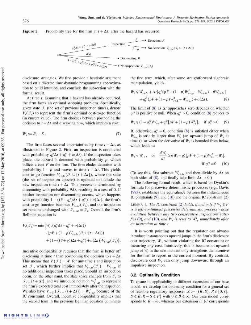
Figure 2. Probability tree for the firm at t +ãt, after the hazard has occurred.

No inspection: Vt+∆t(�t)

1 – ((� + qtn)∆t + qt

m) + o(∆t)

Discounting: 0

InspectionNo detection:1 – p

Detection: Fp

q tn ∆t + q t

m + o(∆t)Vt+∆t (�t {t + ∆t})

�∆t

disclosure strategies. We first provide a heuristic argumentbased on a discrete time dynamic programming approxima-tion to build intuition, and conclude the subsection with theformal result.

At time t, assuming that a hazard has already occurred,the firm faces an optimal stopping problem. Specifically,given state It (the set of previous inspection times), denoteVt4It5 to represent the firm’s optimal cost-to-go function(in current value). The firm chooses between postponing thedecision to t+ãt and disclosing now, which implies a cost:

Wt 2=Rt − St0 (7)

The firm faces several uncertainties by time t+ãt, asillustrated in Figure 2. First, an inspection is conductedwith probability qn

t ãt + qmt + o4ãt5. If the inspection takes

place, the hazard is detected with probability p, whichinflicts a cost F on the firm. The firm eludes detection withprobability 1 − p and moves to time t +ãt. This yieldscost-to-go function Vt+ãt4It ∪ 8t +ãt95, where the state(the set of inspection epochs) is updated to include thenew inspection time t+ãt. This process is terminated bydiscounting with probability �ãt, resulting in a cost of 0. Ifneither inspection nor discounting occurs, which happenswith probability 1 − 44�+ qn

t 5ãt+ qmt 5+ o4ãt5, the firm’s

cost-to-go function becomes Vt+ãt4It5, and the inspectionset remains unchanged with It+ãt =It . Overall, the firm’sBellman equation is

Vt4It5=min8Wt14qnt ãt+qm

t +o4ãt55

·4pF +41−p5Vt+ãt4It∪8t+ãt955

+41−44�+qnt 5ãt+qm

t 5+o4ãt55Vt+ãt4It590

Incentive compatibility requires that the firm is better offdisclosing at time t than postponing the decision to t +ãt.This means that Vt4It5=Wt for any time t and inspectionset It , which further implies that Vt+ãt4It5 = Wt+ãt ifno additional inspection takes place. Should an inspectionoccur, on the other hand, the state space changes from It toIt ∪ 8t +ãt9, and we introduce notation W I

t+ãt to representthe firm’s expected total cost immediately after the inspection.We also have Vt+ãt4It ∪ 8t+ãt95=W I

t+ãt because of theIC constraint. Overall, incentive compatibility implies thatthe second term in the previous Bellman equation dominates

the first term, which, after some straightforward algebraicmanipulation, yields

Wt¶Wt+ãt+ãt6qnt 4pF +41−p5W I

t+ãt−Wt+ãt5−�Wt+ãt7

+qmt 4pF +41−p5W I

t+ã−Wt+ãt5+o4ãt50 (8)

The limit of (8) as ãt approaches zero depends on whetherqmt is positive or null. When qm

t > 0, condition (8) reduces to

Wt¶41−qmt 5Wt++qm

t 6pF +41−p5W It+71 if qm

t >00 (9)

If, otherwise, qmt = 0, condition (8) is satisfied either when

Wt+ is strictly larger than Wt (an upward jump of Wt attime t), or when the derivative of Wt is bounded from below,which leads to

Wt<Wt+1 ordWt

dt¾�Wt−qn

t 6pF +41−p5W It+−Wt71

if qmt =00 (10)

(To see this, first subtract Wt+ãt and then divide by ãt onboth sides of (8), and finally take limit ãt → 0.)

The following formal result, which is based on Dynkin’sformula for piecewise deterministic processes (e.g., Davis1993), establishes the equivalence between the instantaneousIC constraints (9), and (10) and the original IC constraint (2).

Lemma 1. The IC constraint (2) holds, if and only if Wt ¶ Fis a left-continuous piecewise deterministic process whoseevolution between any two consecutive inspections satis-fies (9), and (10), and Wt is reset to W I

t+ immediately afteran inspection at time t.

It is worth pointing out that the regulator can alwaysintroduce instantaneous upward jumps in the firm’s disclosurecost trajectory, Wt , without violating the IC constraint orincurring any cost. Intuitively, this is because an upwardjump of Wt in the next moment only strengthens the incentivefor the firm to report in the current moment. By contrast,disclosure cost Wt can only jump downward through animpulsive inspection.

3.2. Optimality Condition

To ensure its applicability to different extensions of our basemodel, we develop the optimality condition for a general setof feasible regulatory responses L 2= 84R1S52 R∈ 601 r̄71S ¶ B̄1R− S ¶ F 9 with 0 ¶ B̄¶�. Our base model corre-sponds to B̄ = �, whereas our extension in §7 corresponds

Dow

nloa

ded

from

info

rms.

org

by [

152.

3.34

.72]

on

17 M

ay 2

016,

at 0

9:35

. Fo

r pe

rson

al u

se o

nly,

all

righ

ts r

eser

ved.


to B̄ = 0. We first claim that the regulator’s dynamic opti-mization uses Wt as the state variable that summarizes theentire history It . This way of reducing the dimension of thestate space in the dynamic mechanism design problem ispioneered by Spear and Srivastava (1987) and Abreu et al.(1990).

Lemma 2. The regulator’s optimal cost-to-go in time tvalue starting from Wt =w is given by the following time-homogeneous function.

C?4w52= min4Wt 1Rt 1Qt5t¾0

Ɛ

[

∫ �

0e−4�+�5t4�4�Rt−�Wt5+kqn

t 5dt

+k∑

qmt >0

e−4�+�5tqmt �W0 =w

]

(11)

subject to (9)1(10)1 and 4Rt1Rt−Wt5∈L1

for all t¾01

where � 2= 1+�−c/r̄ . In particular, the regulator’s optimalcost is C? 2= 4�/4�+ �55c̄+ minw¶F C

?4w5.

As in the previous section, we first provide a heuristicargument for the recursive formulation of the regulator’sproblem before establishing a formal result on the optimalityconditions.

At time t when Wt =w, the regulator first decides whetherto conduct an impulsive inspection or an upward jump of Wt .If neither is used (i.e., qm = 0 and Wt+ =Wt), the regulatorthen chooses the remediation level r and inspection intensityqn during the next ãt, as well as the firm’s disclosure costwI

+right after an inspection during ãt.9 The regulator’s

optimization problem (11) during this ãt becomes

min4r1r−w5∈L1

wI+¶F 1qn¾0

{

�ãt4�r−�w5+qnãt4k+C?4sI+55

+41−4�+�+qn5ãt5C?4Wt+ãt5+o4ãt5}

=C?4w5+6NC?4w5−��w−4�+�5C?4w5+7ãt+o4ãt51

where operator N is defined as

NC?4w5 2= min4r1 r−w5∈L1

wI+¶F 1qn1 z¾0

��r + qn6k+C?4wI+5−C?4w57

+ 8�w− qn6pF + 41 −p5wI+

−w7+ z9dC?4w5

dw0 (12)

(The equality follows from the first-order Taylor expansionof C?4Wt+ãt5 at state Wt =w, assuming Wt+ãt −Wt =O4ãt5,and IC constraint (10), with slack z = dWt/dt − �w +

qn6pF + 41 −p5wI+

−w7¾ 0.)If impulsive inspection is used (qm > 0), the regulator’s

optimization over decisions qm, wI+

and w+ 2=Wt+ can beexpressed as the following recursive formulation:

MC?4w52= minw+1w

I+¶F 1

qm∈60117

{

qm4k+C?4wI+55+41−qm5C?4w+5

}

(13)

subject to w¶41−qm5w++qm6pF +41−p5wI+71

where IC constraint (9) is enforced in the above constraint.When impulsive inspection qm > 0, it dominates any boundedintensive control qn. Therefore, qn is not a decision variablein this case. Also note that we still allow the feasible set ofqm to start from 0. When qm = 0, the functional operatorM reduces to a simple upward adjustment of the firm’sdisclosure cost level s+ ¾ s.

Overall, the Bellman equation of the regulator’s problem is

C?4w5= min8MC?4w51C?4w5+ 6NC?4w5−��w

− 4�+�5C?4w57ãt + o4ãt591

where the first and second terms correspond to qm > 0and qm = 0, respectively. By rearranging terms and lettingãt go to zero, this further leads to the following optimal-ity condition in the form of quasi-variational inequalities(Bensoussan and Lions 1982):

min8MC?4w5−C?4w51NC?4w5

−��w− 4�+�5C?4w59= 00 (14)

The following Verification Theorem rigorously establishesthe connection between the previous recursive formulationand the original problem.

Theorem 1 (Verification Theorem). Given the feasibleset of regulatory responses L, if C4w5 is a bounded, nonde-creasing, continuous, and differentiable function on 4−�1 F 7that satisfies

MC4w5−C4w5¾ 01

NC4w5−��w− 4�+�5C4w5¾ 01 for w¶ F 1(15)

where functional operators N and M are defined in (12)and (13), respectively, then C4w5 is a lower bound of theoptimal value-to-go function C?4w5 defined in (11).

Note that Theorem 1 only presents conditions for a lowerbound of the optimal value function C?4w5. This is becausecondition (15) does not require that at least one of the twoinequalities holds at equality, as in (14). Our solution strategyin the subsequent sections is to propose an admissible policyand compute its cost-to-go function, which bounds theoptimal cost-to-go from above. We then demonstrate that thecost-to-go function of our proposed policy also satisfies (15),thereby also bounds the optimal cost-to-go from below.

4. Benchmark Policies andPreliminary Insights

Before presenting the optimal regulation policy in §5, wefirst introduce two simple benchmark policies that helpreveal important insights into the optimal policy. These twosimple benchmark policies rely on using only one regulatoryinstrument, either the rewards or the inspections, to uncoverthe hazard.

Dow

nloa

ded

from

info

rms.

org

by [

152.

3.34

.72]

on

17 M

ay 2

016,

at 0

9:35

. Fo

r pe

rson

al u

se o

nly,

all

righ

ts r

eser

ved.


First, note that because of time discounting, the firm hasan economic incentive to postpone the hazard’s disclosure aslong as the corresponding cost is positive and the regulatordoes not inspect the firm. To eliminate such incentive,the regulator needs to dynamically adjust the regulatoryresponses so that the firm’s total cost for disclosing thehazard immediately, Rt − St , is no greater than the presentvalue of the firm’s cost from delaying the disclosure by ãt,that is,

Rt − St ¶ e−�ãt4Rt+ãt − St+ãt50 (16)

In particular, when the regulator always fully covers thefirm’s remediation cost (St ≡Rt), the firm does not incur anycost for disclosing the hazard and hence reports the hazardimmediately. Thus, the regulator should never offer a subsidyamount which is higher than the remediation cost (St >Rt).More crucially, when the regulator does not fully cover theremediation costs (St <Rt), the firm’s total payment Rt − Stneeds to increase over time so as to offset any incentive ofdelaying the hazard’s disclosure (i.e., condition (16) impliesthat Rt+ãt − St+ãt >Rt − St when Rt − St > 0, which canalso be seen from (10) with qn

t = 0). However, the totalcost that the firm can incur is bounded from above by itslimited liability F , so Rt −St cannot increase infinitely. Thus,when inspections are not possible, the regulator can onlyincentivize the firm by covering all remediation costs at alltimes (St ≡Rt). This policy provides our first benchmark.

Proposition 1 (No-Inspection Policy). In the absence ofinspection (i.e., qm

t = qnt = 0 for all t > 0), if c > 41 +�5r̄ ,

the optimal regulation policy for (6) always subsidizes a fullremediation: St = Rt = r̄ for all t ¾ 0. Otherwise, the firm isnot regulated and St =Rt = 0 for all t ¾ 0. Furthermore, theregulator’s cost is equal to �6c̄− 4c− 41 +�5r̄5+7/4�+ �5.

Thus, without inspections, the regulator either fully subsi-dizes a full remediation or does not regulate the firm. Indeed,the total discounted damage reduction that the regulationbrings about is proportional to 4c− 41 +�5r̄5+. This benefit,however, is only positive when c is larger than 41 +�5r̄ . Ifc is too small, regulating the firm is too expensive.

By contrast, our second benchmark policy consists ofrelying on inspections only. Specifically, the reward St iskept at 0, whereas the mandated remediation cost Rt isset at the highest level r̄ , which is feasible only if r̄ ¶ F .As discussed above, this always incentivizes the firm todelay the disclosure of the hazard to a later date. Thus, theregulator can only use the threat of an inspection to uncoverthe hazard. In this case, the regulator should not schedule theinspections but run them randomly, as stated in the followingresult.

Proposition 2 (Inspection-Only Policy). When Rt =

r̄ < F and St = 0 for all t ¾ 0, the optimal regulation policyfor (6) conducts random inspections according to a Poissonprocess with constant rate qn = �r̄/4p4F − r̄ 55. Furthermore,the regulator’s cost is equal to 4�4c̄− c+ r̄ 5+ kqn5/4�+ �5.

Under an inspection-only policy, the regulator prefersrandom intensive inspections because they are cheaper thanimpulsive inspection if Rt − St is maintained constant overtime. To see this, consider any time interval 6t1 t+ãt5. Ifan impulsive inspection with probability qm

t > 0 is used attime t, the inspection cost over this time period (with orwithout intensive inspection) is kqm

t +O4ãt5. By contrast,using intensive inspection with rate qn

t only costs kqnt ãt,

which is on the order of O4ãt5.Furthermore, the optimal intensity qn

t remains constant overtime for the inspection-only policy. Indeed, intensity qn

t needsto ensure that the benefit from delaying the disclosure (andhence the remediation payment) for a small time interval ãt,which is �ãtr̄ + o4ãt5, is offset by the expected penalty ofbeing caught, which is qn

t ãt×p4F − r̄ 5+ o4ãt5. That is,inspection intensity qn

t is set such that �r̄ãt = qnt ãtp4F − r̄ 5,

which corresponds to the binding IC constraint (10).

5. Optimal Regulation Policy with AccurateInspections 4p = 15

We now present our main result, which characterizes theoptimal regulation policy of (6) when inspections are accurate(p = 1). As described in the following theorem, the optimalpolicy features a simple cyclic deterministic structure. This isin sharp contrast with the previous two benchmark policies.

Theorem 2. When inspection accuracy is perfect (p = 1),the optimal regulation policy is determined by time t?, theunique positive solution of the following equation:

��F 41−e−4�+�5t?5=4�+�564k+�F 541−e−�t?5−k70 (17)

The policy inspects the firm periodically at deterministic timeepochs �i = t? × i, for i = 1121 0 0 0 with qm

�i

? = 1, qm?t = 0 for

t 6= �i and qn?t = 0 for t ¾ 0. Let �0 = 0.

• If c > 41 +�5r̄ , a full remediation is mandated withR?

t = r̄ for t ¾ 0, and the reward follows

S?t = r̄ − Fe�4t−�i51 for t ∈ 4�i−11 �i71

with S?�i−1+

= s̄? 2= r̄ − Fe−�t? and S?�i

= r̄ − F 0(18)

• If c ¶ 41+�5r̄ , no remediation is mandated with R?t = 0

for t ¾ 0, and the reward follows

S?t = −Fe�4t−�i51 for t ∈ 4�i−11 �i71

with S?�i−1+

= s̄? 2= −Fe−�t? and S?�i

= −F 0(19)

Finally, the regulator’s optimal cost at time 0 is

C?=

�

�+ �6c̄− 4c− 41 +�5r̄5+ −�Fe−�t? 70 (20)

Figure 3 depicts the cyclic structure of the optimal policywhen the damage reduction from a full remediation is largeenough (c > 41 +�5r̄). The remediation level R?

t is set at

Dow

nloa

ded

from

info

rms.

org

by [

152.

3.34

.72]

on

17 M

ay 2

016,

at 0

9:35

. Fo

r pe

rson

al u

se o

nly,

all

righ

ts r

eser

ved.


Figure 3. The optimal regulation policy with perfect inspection (p= 1) and c > 41 +�5r̄ for c = 10, �= 003, r̄ = 6,F = 12, k = 006, �= 002, and � = 1.

t

$

St

0

�1 �2 �3 �4 �5 �6

Scheduled inspections

t t t t t t

Rtr̄

s̄

r – F¯

its upper bound r̄ , and the reward level S?t decreases from

s̄? ¶ r̄ to r̄ − F between two consecutive inspections.Thus, the optimal regulation policy always mandates a full

remediation as in the noninspection policy of Proposition 1.(In fact, the noninspection policy is essentially the limitingcase of the optimal policy for infinitely large inspectioncost, since t? approaches infinity as k increases to infinity,according to (17).) However, although the noninspectionpolicy fully subsidizes the firm’s remediation cost (withSt = r̄ for all t), the optimal policy in Theorem 2 decreasesthe reward level St below r̄ . This dynamic adjustmentreduces the regulator’s cost and exactly offsets the firm’sincentive to delay the hazard’s disclosure, as explained in §4(in particular, trajectory (18) guarantees that (16) holds atequality). The reward amount continues to decrease untilthe firm’s total disclosure cost reaches the firm’s liability,i.e., Rt − St = r̄ − St = F . At this point, the regulator canno longer increase the firm’s cost. Instead, the regulatorruns an inspection that resets St to s̄?, which also starts thenext cycle. This is in contrast with the noninspection policy,under which the regulator cannot circumvent the firm’sliability constraint with an inspection. And in contrast withthe inspection-only policy of Proposition 2, the regulatordoes not run any random inspections but instead follows aperiodic inspection schedule.

Figure 4 depicts the optimal policy when the damagereduction of a full remediation is small (c¶ 41 +�5r̄). Theoptimal policy retains the same structure, except that bothRt and St are shifted downward. Specifically, the regulatornever mandates a repair with Rt = 0; and the reward amountSt decreases from a negative value s̄? all the way to −F , atwhich point an inspection takes place.

To understand this difference, note first that the reducedenvironmental damage c does not directly affect the firm’sincentive to disclose the hazard (c does not appear in the(IC) constraint (2)). What matters to the firm is the totalcost Rt − St of disclosing the hazard at time t. How thistotal cost is split between the mandated remediation levelor the reward is irrelevant to the firm. This is not the case,however, for the regulator. As in Proposition 1, a remediationis too expensive to society and Rt = 0 if c < 41 + �5r̄ .Since St needs to be lower than Rt (as discussed in §4), thereward amount is always negative in this case. Therefore, thereward corresponds to a reduced fine, with 0 ¾ St ¾−F . Bycontrast, mandating a full remediation is always optimal ifc > 41 +�5r̄ . In this case, and if s̄? > 0, the reward amountsatisfies r̄ ¾ St ¾ 0 during the early phase of a policy cycle.The reward corresponds then to a (partial) subsidy for a fullremediation, which results in net cost r̄ − St ¾ 0 for the firm.

Overall, Theorem 2 demonstrates how the use of inspec-tions enables the regulator to incentivize the firm with adecreasing reward level. In fact, the theorem also revealsthe impact of these inspections on social cost. Specifically,the optimal cost C? is exactly equal to the cost of the no-inspection policy in Proposition 1, minus a term proportionalto �Fe−�t? . Thus, this last term captures the reduction insocial cost that inspections bring about.

Furthermore, Theorem 2 reveals how the size of the rewardlevel is related to the frequency of inspection. Specifically,reward threshold s̄? given in (18) and (19) is increasingin t?. Thus, to reduce the inspection costs, the regulatorneeds to trade off less frequent inspections (i.e., longer t?)with higher rewards (i.e., higher values of s̄?). The optimal

Dow

nloa

ded

from

info

rms.

org

by [

152.

3.34

.72]

on

17 M

ay 2

016,

at 0

9:35

. Fo

r pe

rson

al u

se o

nly,

all

righ

ts r

eser

ved.


Figure 4. The optimal regulation policy with perfect inspection (p = 1) and c ¶ 41 +�5r̄ for c = 5, �= 003, r̄ = 6, F = 12,k = 006, �= 002, and � = 1.

t t t t t t�1 �2 �3 �4 �5 �6


St

t

Rt ≡ 0$

0

s̄

–F

trade-off is reflected in (17), which can be thought of as afirst order optimality condition for the cycle length t?.

Finally, Theorem 2 points out the importance of the firm’slimited liability in the optimal regulation policy. In fact, thenext result shows that the key parameters of the optimalpolicy are monotone in F .

Corollary 1. Ceteris paribus, both s̄? and t? are decreas-ing in F .

In particular, since t? is decreasing in F , the cost reduction�Fe−�t? increases in F . In other words, the social benefitof using inspections increases with the firm’s liability, asshould be expected.

Figure 5 illustrates this points numerically and depicts theeffect of the firm’s limited liability F on the key parametersof the reward and inspection policies specified in Theorem 2.The corollary shows that higher liability F allows theregulator to apply more stringent reward policies and thusreduces s̄?. In essence, as the firm’s ability to pay forenvironmental hazard increases, the regulator is able to offerlower rewards.

Perhaps more surprising, however, is the effect of the firm’sliability on the regulator’s inspection policy. Corollary 1suggests that the inspection frequency, 1/t?, increases with F .It appears that Kim (2015) is the first and only study todemonstrate the potential complementarity of the firm’slimited liability and inspections. Nonetheless, the rationalebehind our result differs from Kim’s (2015), whereby thecomplementarity emerges when the firm has incentives tocheat. In his setting, a higher firm’s ability-to-pay induces theregulator to increase the inspection frequency to detect more

hazards and hence generate more revenues from penalties. Inour setting, however, a rational firm never cheats under theoptimal policy and, therefore, the maximum penalties (equalto the firm’s liability) are never collected in equilibrium(or only collected when the hazard happens to occur at thescheduled inspection epochs, which are zero-probabilityevents). Nevertheless, higher firm liability strengthens thepower of the regulator’s threat and hence improves theeffectiveness of inspections in inducing voluntary disclosures.This allows the regulator to use inspections more frequently(i.e., to lower t?) so as to decrease the reward levels (i.e., tolower s̄? and hence St).

Proof of Theorem 2

We conclude this section by outlining the main steps toprove Theorem 2, which also provide the logic of the moreintricate proofs for the extensions of the base model in thenext two sections. The proof derivations for the major stepsare presented in Appendix B.

First, we verify that t? is well-defined according to (17).

Lemma 3. There exists a unique solution t? > 0 to (17).

We then verify that the policy prescribed in Theorem 2 isindeed incentive compatible.

Proposition 3. Under the policy prescribed in Theorem 2,the firm’s total cost upon disclosure, is given by

W ?t =R?

t − S?t = Fe�4t−�i51

for t ∈ 4�i−11 �i71 i = 1121 0 0 0 1 (21)

which satisfies (9), and (10) with p = 1.

Dow

nloa

ded

from

info

rms.

org

by [

152.

3.34

.72]

on

17 M

ay 2

016,

at 0

9:35

. Fo

r pe

rson

al u

se o

nly,

all

righ

ts r

eser

ved.


Figure 5. The effect of the firm’s limited liability (F ) on the optimal regulation policy with p = 11 c = 101�= 0031 r̄ =

61 k = 0061�= 002, and � = 1.

6 8 10 12 14 16

2

3

4

5

F

6 8 10 12 14 161.2

1.4

1.6

1.8

2.0

2.2

F

(a) Reward threshold s̄ (b) Inspection periodicity t

Next, we derive the cost-to-go function under the policyprescribed in Theorem 2.

Proposition 4. The regulator’s cost-to-go function underthe policy specified in Theorem 2 is given by

C4w5 2= −�

�+ �6c− 41 +�5r̄7+ +

k+�F 41 − e−�t?5

F 4�+�5/�41 − e−4�+�5t?5

·w4�+�5/�−�w1 for w ∈ 6Fe−�t?1 F 71 (22)

which is strictly, convex increasing with

C4Fe−�t?5= −�

�+ �86c− 41 +�5r̄7+ +�Fe−�t?91

anddC4w5

dw

∣

∣

∣

∣

w=Fe−�t?

= 01(23)

Since the policy specified in Theorem 2 is admissible, cost-to-go function C4w5 is an upper bound of the optimal cost-to-go function, C?4w5. The next result demonstrates thatcost-to-go function C4w5 satisfies the sufficient conditionof Theorem 1, which is, therefore, also a lower bound ofC?4w5.

Proposition 5. Extend function C4w5 defined in (22) bydefining C4w5 ≡ C4Fe−�t?5 for w ¶ Fe−�t? . Then C4w5satisfies (15) with equalities for w ∈ 6Fe−�t?1 F 7. ThereforeC?4w5=C4w5 for w ∈ 6Fe−�t?1 F 7.

Thus, C4w5= C?4w5, and the policy is optimal, completingthe proof of the optimality of the policy in Theorem 2. Inparticular, since W ?

0 = Fe−�t? minimizes C4w5, Lemma 2suggests that the regulator’s expected cost at time 0 isC? = c̄�/4�+ �5+C4Fe−�t?5, which is essentially (20).

6. Optimal Regulation Policy withInaccurate Inspections 4p¶ 15

When inspections are inaccurate (p < 1), the optimal policyretains the same cyclic structure as with accurate inspection

(p = 1), except for the very first cycle. Indeed, the followingtheorem shows that when p < 1, the first inspection takesplace after a longer time period than the subsequent ones.The reward amount is then set at its highest possible level atthe beginning of the time horizon (t = 0). Furthermore, thereward amount is set such that the firm’s total cost neverreaches liability F .

Theorem 3. The optimal regulation policy is determined bya single parameter, t?, which is the unique positive solutionto the following equation:

��pF 41−e−4�+�5t?5=4�+�541−41−p5e−�t?5

·

[(

k

p+�F

)

41−e−�t?5−k

]

0 (24)

Then the regulator inspects only at time epochs �i = t?0 +

4i− 15t?, for i = 1121 0 0 0 1 where

t?0 2= −1�

ln(

1 −1 − e−�t?

p

)

¾ t?0 (25)

Namely, qm�i

? = 1, qm?t = 0 for t 6= �i and qn?

t = 0 for t ¾ 0.Let F̂ 2= pF /61 − 41 −p5e−�t? 7 and �0 = 0.

• If c > 41 + �5r̄ , we have R?t = r̄ for all t ¾ 0, and

S?t = r̄ − F̂ e�4t−�i5 for t ∈ 6�i−11 �i7, with

S?0 = s?0 2= r̄ − F̂ e−�t?0 ¾ S?

�i+= s̄? 2= r̄ − F̂ e−�t?

>S?�i

= s? 2= r̄ − F̂ ¾ r̄ − F 0 (26)

• If c ¶ 41 + �5r̄ , we have R?t = 0 for all t ¾ 0, and

S?t = −F̂ e�4t−�i5 for t ∈ 6�i−11 �i7, with

S?0 = s?0 2= −F̂ e−�t?0 ¾ S?

�i+= s̄? 2= −F̂ e−�t?

>S?�i

= s? 2= −F̂ ¾−F 0 (27)

Dow

nloa

ded

from

info

rms.

org

by [

152.

3.34

.72]

on

17 M

ay 2

016,

at 0

9:35

. Fo

r pe

rson

al u

se o

nly,

all

righ

ts r

eser

ved.


Figure 6. The optimal regulation policy with imperfectinspection (p = 005) and c > 41 +�5r̄ for c =

101�= 0031 r̄ = 61 F = 121 k= 0061�= 002,and � = 1.

0

r̄

$

s̄

s0

s¯

r – F¯

t

St

Rt

t0 t

t

t t t t�1 �2 �3 �4 �5 �6


∨

All nonstrict inequalities in (25)–(27) hold as equalities ifand only if p = 1. Finally, the regulator’s optimal cost is

C?=

�

�+ �8c̄− 4c− 41 +�5r̄5+ −�F̂ e−�t?090 (28)

Figure 6 depicts an example of the optimal policy forinaccurate inspection (p < 1) when the damage reductionfrom a full remediation is sufficiently large (c > 41 +�5r̄).For each cycle, the lower reward threshold s? is larger thanr̄ − F , with the first cycle starting from a higher rewardlevel s?0 > s̄? and taking a longer time t?0 > t? before the firstinspection.

The choices of reward thresholds s̄? and s? reflect that theIC constraint (9) associated with impulsive inspections isbinding at the optimum. Specifically, consider the firm’strade-off between immediately reporting a hazard that occursright before an inspection, and delaying the disclosure of thehazard until right after the inspection. The expected benefitof waiting until after the inspection is 41 −p5s̄?, whereas theexpected penalty cost is pF . Thus, the reward for disclosingright before an inspection has to satisfy s? ¶ 41 −p5s̄? −pF ,which corresponds to the IC constraint (9) for qm? = 1. Thisinequality holds at equality for s̄? and s? specified in (26).By contrast, when inspections are perfectly accurate, thefirm cannot expect a benefit for disclosing the hazard rightafter the inspection. Indeed, the inspection always revealsthe hazard in this case and 41 −p5s̄? = 0 when p = 1 so thatthe lower threshold s? is set at the lowest possible boundallowed by the firm’s liability (i.e., r̄ − F if c > 41 +�5r̄and −F otherwise).

This also explains why the first cycle is longer than thesubsequent ones. Indeed, as discussed above, the regulatorshould not set s̄? to too high a level so as to offset the firm’sincentive to take the chance of slipping through an inaccurateinspection. But such a concern is not present when t = 0,which leads to a higher s̄?0 and hence a longer first cycletime t?0 .

Furthermore, Theorem 3 reveals an important connectionbetween the regulator’s inspection accuracy and the firm’slimited liability. In short, inaccurate inspections weaken theregulator’s power but strengthen the firm’s position. This isreflected by the maximum possible cost that the regulatoractually imposes on the firm. Indeed, the optimal policyin Theorem 3 for p < 1 resembles that of Theorem 2 forp = 1, if F̂ is replaced with F . (This can be readily seen bycomparing (18) and (19) with (26) and (27), respectively.)Since F̂ ¶ F with the equality holding only when p = 1,the effect of inaccurate inspections acts as if the firm’sliability is decreased and, as a result, the firm’s position isstrengthened. As such, the regulator’s total cost given by(28) becomes higher than that given by (20).

Overall, Theorem 3 points to the importance of inspectionaccuracy in optimal regulation policy. As shown in thenext result, the key parameters of the optimal policy are allmonotone in p.

Corollary 2. Ceteris paribus, s?0 , s? and t?0 decreases in p,while t? increases in p.

Figure 7 illustrates Corollary 2 and depicts the effect ofaccuracy p on the parameters of the reward and inspectionpolicies as described in Theorem 3. In particular, the inspec-tion frequency, 1/t?, increases as inspections become lessaccurate (i.e., as p decreases), compensating for the lackof accuracy. A lower accuracy level p is also compensatedfor by a higher initial reward s?0 and thus a longer firstcycle t?0. Indeed, because a lower accuracy level requiresmore frequent, and hence more expensive inspections, theregulator seeks to postpone the use of inspections altogetherby increasing t?0 . Similarly, the regulator also offers a higherreward threshold s? for a lower level of accuracy. However,in general, s̄? is not monotonic for p < p?, as illustratedin Figure 7(a). (Our numerical experiments (not reported)show that s̄? is either monotonic or first decreasing and thenincreasing in p.)

Note finally that the effect of the firm’s liability F for p = 1in Corollary 1 also holds when p < 1 (see Proposition EC.5of the e-companion).

7. Optimal Regulation Policy withFrictionless Fine 4�= 01St ¶ 05

Thus far, we have assumed that each dollar spent by theregulator is raised through distortionary taxes that are costlyto society. This corresponds to a positive shadow costof public funds with � > 0 for the regulator. When theapplication of public funds is frictionless (�= 0), the use

Dow

nloa

ded

from

info

rms.

org

by [

152.

3.34

.72]

on

17 M

ay 2

016,

at 0

9:35

. Fo

r pe

rson

al u

se o

nly,

all

righ

ts r

eser

ved.


Figure 7. (Color online) The effect of the inspection accuracy (p) on the optimal regulation policy with c = 10, �= 003,r̄ = 6, F = 12, k = 006, �= 002, and � = 1.

0 0.2 0.4 0.6 0.8 1.0

0

5

p0 0.2 0.4 0.6 0.8 1.0

p

Rew

ard

thre

shol

ds(a) Reward policy

0

2

4

6

8

Peri

odic

ity

(b) Inspection policy

–5s0s̄s

t0t

of subsidies is “free of charge” to the regulator, who canthen offer an infinitely large subsidy to reward voluntarydisclosure. The regulator can induce the firm to promptlyreveal the hazard at no cost, and the design of the regulationpolicy becomes trivial, as stated in the next result.

Corollary 3. If �= 0, the optimal regulation policy con-ducts no inspections at all and fully reimburses the firm’sremediation cost, if any (i.e., S?

t =R?t for all t ¾ 0), upon

disclosure. In particular, if c > r̄ , a full remediation is man-dated upon disclosure, i.e., R?

t = r̄ for all t ¾ 0; otherwise,no remediation is mandated upon disclosure, i.e., R?

t = 0 forall t ¾ 0. Furthermore, the regulator’s optimal cost is equalto C? = �6c̄− 4c− r̄ 5+7/4�+ �5.

Thus, if the damage reduction is worth its cost (c > r̄),the regulator fully subsidizes a full remediation. Otherwise,the firm is not regulated.

However, subsidies may not be allowed in practice (EPA2001). As such, the regulator cannot offer any positivereward to the firm and can only fine the firm when the hazardis disclosed. In our setup, this corresponds to restrictingthe reward amount to nonpositive values, i.e., St ¶ 0. Inother words, when �= 0 and St ¶ 0, the frictions associatedwith the application of public funds takes the form of anupper bound at 0 on the reward amount. In this case, theregulator’s problem becomes

C? 2=�

�+ �c̄+ min

RƐ

[

e−�T 41 − c/r̄5RT +K∑

�i∈IQT

e−��i

]

1

subject to (2) and St ¶ 00 (29)

When positive rewards are not allowed, the next theoremshows that the optimal policy retains a cyclic structure, inwhich the dynamic adjustment of mandated remediationlevel sometimes acts as a substitute for the subsidy.

Theorem 4. Suppose �= 0, St ¶ 0 for t ¾ 0 and p = 1. Ifc¶ r̄ , the optimal regulation policy does not regulate thefirm, i.e., Rt = St = qm

t = qnt = 0 for all t. Otherwise, the

optimal regulation policy is characterized by time t?, whichis the unique solution to the following equation,

�e−4�+�5t?−

[

�

(

min{

r̄

F11})−�/�

+�

(

min{

r̄

F11})

+ 4�+ �5r̄

F

K

c− r̄

]

e−�t?+ � = 01 (30)

such that t? > t̄ 2= 641/�5 ln4F /r̄57+. The regulator inspectsthe firm periodically at deterministic time epochs �i = t? × ifor i = 1121 0 0 0 1 with qm?

�i= 1, qm?

t = 0 for t 6= �i and qn?t = 0

for t ¾ 0. Then,

R?t = Fe−�4�i−t51 S?

t = 01 for t ∈ 4�i−11 �i − t̄ 73

R?t = r̄ 1 S?

t = r̄ − Fe−�4�i−t51 for t ∈ 4�i − t̄1 �i71(31)

with R?�i−1+

= r? 2= Fe−�t? and S?�i

= −4F − r̄ 5+. Finally, theregulator’s optimal cost at time 0 is

C?=

�

�+ �8c̄− 4c/r̄ − 15+Fe−�t?90 (32)

Figure 8 illustrates the optimal policy described in Theo-rem 4. The policy retains a deterministic cyclic structure,where scheduled inspections are performed periodically.In contrast to the previous cases, however, the optimalpolicy dynamically adjusts the remediation level upon thedisclosure. Specifically, at the beginning of each cycle, theregulator wishes to dynamically adjust a subsidy (i.e., apositive reward) to the firm for self-reporting the hazard.But because subsidies are not allowed, the regulator insteadresorts to adjusting the mandated remediation level (up to thefull repair r̄). To emulate a decrease in the subsidy amount,

Dow

nloa

ded

from

info

rms.

org

by [

152.

3.34

.72]

on

17 M

ay 2

016,

at 0

9:35

. Fo

r pe

rson

al u

se o

nly,

all

righ

ts r

eser

ved.


Figure 8. The optimal regulation policy with �= 0, St ¶ 0, c > r̄ and r̄ ¶ F for p = 1, r̄ = 6, F = 12, k = 006, �= 002,and � = 1.

t t t t t t�1 �2 �3 �4 �5 �6


t- t- t- t- t- t- t0

r̄

¯r

r – F¯

$

Rt

St

the regulator needs to increase the remediation level. In thissense, the regulator uses the remediation level as a substitutefor subsidies. This allows the regulator to gradually decreasethe firm’s total cost Rt − St so as to incentivize the firm todisclose the hazard immediately, as discussed in §4.

When the remediation level acts as a substitute for asubsidy, the regulator faces a new tradeoff between reducingregulatory costs and limiting the reduction of environmentaldamage. That is, the level of c also affects the frequency ofinspection 1/t?, which is in contrast with the case �> 0discussed in §5. The following corollary formally examinesthe effect of maximum damage reduction c. Recall fromTheorem 4 that the firm is not regulated when c¶ r̄ .

Corollary 4. Ceteris paribus, t? is decreasing in c > r̄while r? is increasing in c > r̄ .

Figure 9 illustrates the result in Corollary 4. Fixing r̄ ,the environmental cost associated with a low remediationlevel (Rt < r̄) increases with c. The regulator, therefore, setsthe minimum level of mandated repairs r? to a higher levelfor higher c. This reduces the regulator’s ability to use theremediation level as a substitute for a subsidy. Thus, theregulator resorts instead to more frequent inspections withshorter cycle length t?.

8. Discussions and ConclusionThis paper proposes a dynamic mechanism design frameworkto study voluntary disclosure of environmental hazards. Thisframework is adequate when the occurrence of the hazardis beyond the firm’s control and privately known only to

the firm, and when the regulatory responses, costly to thefirm, discourage it from revealing on this information. Theapproach enables us to explicitly account for the timing ofthe uncertain event, without a priori restricting the possibleset of admissible inspection and reward policies. Despitethe generality and complexity of our framework, we obtainsimple and easy-to-implement optimal regulation policies inclosed-form. The optimal structure reveals that the regulatorshould rely on offering a reward for a voluntary disclosurefor as long as possible before resorting to an inspection.

Our results critically depend on three “first principles” inour model: private information, limited liability, and frictionsof applying public funds. Without any one of these threeprinciples, the misalignment of incentives, which constitutesthe core of our problem, does not exist in the first place. Inparticular, to the extent that the private information in oursetting is the timing of an event, our problem is, in essence,dynamic.

Our model can be generalized in several meaningfuldirections. First, our model can easily capture the situationunder which the hazard cannot be concealed forever. Instead,if the hazard is inevitably observable by the public some timeafter its occurrence—say, after an exponentially distributedtime—then we only need to generalize the model to allowthe firm’s time discount factor to be different from theregulator’s. The solution procedures in our current modelremain applicable, and the corresponding optimal regulationpolicy, although more complex, retains the same qualitativestructure as demonstrated in this paper. Along this lineof thought, our model can be easily extended to studyregulations that prevent environmental disasters, which may

Dow

nloa

ded

from

info

rms.

org

by [

152.

3.34

.72]

on

17 M

ay 2

016,

at 0

9:35

. Fo

r pe

rson

al u

se o

nly,

all

righ

ts r

eser

ved.


Figure 9. The effect of the environmental damage reduction from full remediation (c > r̄) on the optimal regulation policywhen only fines (St ¶ 0) are allowed with �= 01 r̄ = 61 F = 121 k = 0061�= 002, and � = 1.

6 8 10 12 14 160

1

2

3

4

5

c6 8 10 12 14 16

c

1.0

1.5

2.0

2.5

3.0

3.5

(a) Remediation threshold r¯

(b) Inspection periodicity t

occur some time after a certain risk indicator becomesnoticeable only to the firm.

Furthermore, the main driver of our deterministic cyclicstructure is that the cost to the firm for hiding the hazard—and hence for being caught by an inspection—is equal to thefirm’s limited liability. In some situations, a hazard exposedby an inspection incurs additional intangible costs to thefirm, such as a loss of reputation or public goodwill. Inthis case, the total cost for being caught by an inspection iseffectively higher than the firm’s financial liability. Thesecases constitute interesting extensions of our work, wherethe optimal inspections may, in fact, be random.

To capture the essential tradeoff between environmentaland remediation costs, we make the simplified technicalassumption that the reduced damage c is linear in theremediation cost R. If this relationship is nonlinear, theoptimal remediation level may not be set at an extremevalue (either the lower bound 0 or the upper bound r̄), butsomewhere in between. Furthermore, the optimal solutionmay involve dynamically adjusting the remediation level aswe find in our extension, where subsidies are infeasible.

Finally, we focus in this paper on adverse selectionproblems and thus consider unintentional hazards. In somesettings, the firm can take additional actions to reducethe chance of the hazard, or make costly efforts to elicitinformation about its occurrence. These issues give riseto moral hazard problems. Combining dynamic adverseselection and moral hazard issues is, however, notoriouslydifficult and often intractable. Nonetheless, the closed formsolutions we derive in this paper provide a promising startingpoint for future investigations in this direction.

Supplemental Material

Supplemental material to this paper is available at http://dx.doi.org/10.1287/opre.2016.1476.

Acknowledgments

The authors appreciate discussions with Sang-Hyun Kim andhelpful comments and suggestions from the review team.

Appendix A. Definition of Inspections andRevelation Principle

In this section, we use Xt to denote the corresponding environmentalstate: the state is normal, i.e., Xt = 1, if and only if t < T andthe state is hazardous, i.e., Xt = 0, otherwise. We use Yt ∈ 80119to denote the result of an inspection at time t. According to ourmodel setup, we have

�6Yt = 0 �Xt = 17= 01 �6Yt = 0 �Xt = 07= p0 (A.1)

We notice that the more precise way of writing the right-hand sideof the IC constraint Ɛ6DR

t 4t′5 �It7 is Ɛ6DR

t 4t′5 �It1Xt = 07.

We use IQ6t11 t27

to denote the set of inspection time epochsduring 6t11 t27 under the inspection policy Q. To be consistentwith the notation in the main text, we denote IQ

t 2=IQ601 t7 and

IQ 2=IQ601�5. We define the corresponding counting process as

NQt 2=

∑

�6�i∈I

Qt 7

and the filtration generated by NQt as ¦t . Let

ZQ6t1 �5 2=

∏

�i∈IQ6t1 �5

Y�i for any � ¾ t be the indicator of whether the

firm has survived inspections during time 6t1 �5. That is, ZQ6t1 �5 = 1 if

no inspection takes place (ZQ6t1 �5 is an empty product) or any possible

inspections during time 6t1 �5 produces “no hazard” results (becauseof imperfection of the inspection technology), and ZQ

6t1 �5 = 0 if aninspection during 6t1 �5 correctly identified the hazard. If a hazardis detected at time � , we must have ãZQ

6t1 �7 2= ZQ6t1 �7 −ZQ

6t1 �5 = −1.

Definition A.1 (Inspection Policy). Let dt and �t denote theusual Lebesgue measure and Dirac measure on time horizont ∈ 601�5, respectively. We call 8qn

t ∈ 601�52 t¾ 09 and 8qmt ∈

601172 t ¾ 09 an intensity inspection policy and an impulsiveinspection policy, respectively, if

1. the process qnt and qm

t are ¦t-predictable;2. the measure �4dt5 2= qn

t dt + qmt �t satisfies

∫ t

0�4ds5 <�1 t ¾ 03 and (A.2)

Dow

nloa

ded

from

info

rms.

org

by [

152.

3.34

.72]

on

17 M

ay 2

016,

at 0

9:35

. Fo

r pe

rson

al u

se o

nly,

all

righ

ts r

eser

ved.




3. the measure �4dt5 consists of an ¦t-predictable compensator(c.f. Brémaud 1981, Liptser and Shiryaev 2010) for the countingprocess NQ

t , i.e.,

Ɛ

[

∑

t∈601�5

AtãNQt

]

= Ɛ

[

∫ �

0At�4dt5

]

(A.3)

for any bounded ¦t-predictable process At . �

To establish the most general version of the Revelation Principlethat is applicable to all our settings, we consider a general feasibleset of regulatory responses L 2= 84R1S52 R ∈ 601 r̄ 71 S ¶ B̄1R−S ¶F 9 with 0 ¶ B̄¶�.

Lemma A.1 (Revelation Principle). It is without loss of gener-ality to restrict the search for the optimal regulation policy withinthe class of direct revelation policies. Namely, for an arbitraryregulation policy R̂, there exists an alternative regulation policyR, which is payoff-equivalent to the firm without increasing theregulator’s expected cost. In particular, one can choose policy R,under which it is optimal for the firm to disclose the hazard once itoccurs. Moreover, such policy R 2= 4Rt1 St1Qt5t∈601�5 satisfies theIC constraint (2) with

DRt 4t

′5= −F∑

�∈6t1 t′5

e−�4�−t5ãZQ6t1 �7

+ e−�4t′−t5ZQ6t1 t′54Rt′ − St′ 51 ∀ t′ > t0 (A.4)

Proof. See Appendix EC.1. �

Appendix B. Proofs in §5

Proof of Lemma 3. Let f 4t5 2= ��F +��Fe−4�+�5t −4�+�54�F +

k5e−�t . Then, (17) is equivalent to f 4t?5= 0. The existence anduniqueness of t? thus follow from the straightforward verificationthat f 405= −4�+ �5k < 0, f 4�5= ��F > 0, and

f ′4t5= �4�+ �5e−�t4k+�F −�Fe−�t5¾ �4�+ �5ke−�t > 01

because e−�t ¶ 1. �

Proof of Proposition 3. By definition, W ?t =R?

t − S?t for t ¾ 0.

Thus, (21) follows immediately from (18) and (19). In particular,we have W ?

�i= F and W ?

�i+= Fe−�t? for i = 1121 0 0 0 0

According to the policy prescribed in Theorem 2, impulsiveinspections, qm?

�i= 1, are used only at �i = t?× i. It is straightforward

to verify that,

W ?�i

= F = 41 − 15 · Fe−�t?+ 1 · F

= 41 − qm?�i5W ?

�i++ qm?

�i61 · F + 41 − 15 ·W I?

�i+70

Namely, (9) holds with equality at those inspection epochs.For any other time moments, no impulsive inspection is used in

the policy prescribed in Theorem 2. Thus, we just need to check(10). Indeed, for t ∈ 4�i−11 �i7 and any i, (21) implies that

dW ?t

dt= �W ?

t 1

which is essentially the binding constraint (10) because qn?t ≡ 0 for

all t ¾ 0. �

Proof of Proposition 4. By (21), W ?t , starting from W ?

0 =w ¶ w̄?,takes �14w5 2= 41/�5 ln4F /w5 to reach the upper threshold F whenthe first inspection takes place. Subsequent inspections take placeat �i4w5= �14w5+ 4i− 15t? for i = 2131 0 0 0 1 where t? is given bythe solution to (17).

According to the policy specified in Theorem 2, R?t ≡ r̄�6c¾

41 + �5r̄7 and qn?t ≡ 0 for t ¾ 0, and qm?

t = 1 if t = �i4w5 fori = 1121 0 0 0 but qm?

t = 0 otherwise, implying the correspondingregulator’s cost-to-go function to be, by (11),

C4w5=−�

�+�6c−41+�5r̄7+

+Ɛ

[

∫ �

0e−4�+�5t4−��W ?

t 5dt+k�∑

i=1

e−4�+�5�i4w5

∣

∣

∣

∣

W ?0 =w

]

︸︷︷︸

2= C̃4w5

0

Taking advantage of the cyclical structure of the policy specified inTheorem 2, we compute

C̃4w5=

∫ �14w5

0e−4�+�5t4−��we�t5dt + e−4�+�5�14w5C̃4F 5

= �4e−��14w5 − 15+

(

w

F

)4�+�5/�

C̃4F 5

=C̃4F 5+�F

F 4�+�5/�w4�+�5/�

−�w0 (B.1)

Since a deterministic inspection is conducted once W ?t = F and

W ?t is instantaneously adjusted to Fe−�t? , we must have

C̃4F 5= k+ C̃4Fe−�t?5

= k+ e−4�+�5t? 6C̃4F 5+�F 7−�Fe−�t? 1

where we use (B.1) to compute C̃4Fe−�t?5 and obtain the lastequality above. We solve from the above equality for

C̃4F 5+�F

F 4�+�5/�=

k+�F 41 − e−�t?5

F 4�+�5/�41 − e−4�+�5t?51

which implies that

C̃4w5=k+�F 41 − e−�t?5

F 4�+�5/�41 − e−4�+�5t?5w4�+�5/�

−�w1

and subsequently (22).It is easy to see that 4k + �F 41 − e−�t?55/4F 4�+�5/�41 −

e−4�+�5t?55 > 0. By noting that 4�+ �5/� > 1, we immediately haveC4w5 defined in (22) is strictly convex in w ∈ 601 F 7. Straightforwardcalculation yields

d

dwC4Fe−�t?5

=�+ �

�

k+�F 41 − e−�t?5

F 4�+�5/�41 − e−4�+�5t?5F �/�e−�t?

−�

=4�+ �54k+�F 5e−�t? −��Fe−4�+�5t? −��F

�F 41 − e−4�+�5t?5= 01

which follows from (17). Therefore, we obtain the second equalityin (23) and that C4w5 is strictly increasing in w ∈ 6Fe−�t? 1 F 7.

Dow

nloa

ded

from

info

rms.

org

by [

152.

3.34

.72]

on

17 M

ay 2

016,

at 0

9:35

. Fo

r pe

rson

al u

se o

nly,

all

righ

ts r

eser

ved.


Finally, to see the first equality in (23), we note that

C4w5= −�

�+ �6c− 41 +�5r̄7+

+k+�F 41 − e−�t?5

F 4�+�5/�41 − e−4�+�5t?5w4�+�5/�

−�w

= −�

�+ �86c− 41 +�5r̄7+ +�w9

+�

�+ �w

d

dwC4w50 �

Proof of Proposition 5. In this proof, we denote w? = Fe−�t? < F

and

K? 2=k+�F 41 − e−�t?5

F 4�+�5/�41 − e−4�+�5t?50 (B.2)

Then, the extended function C4w5 defined in the proposition can berewritten as

C4w5=

−�

�+�6c−41+�5r̄7+

+K?w4�+�5/�−�w1 for w∈ 6w?1F 71

C4w?51 for w¶w?1

(B.3)

where C4s?5 is given by (23).By Proposition 4, C4w5 defined above is bounded, nondecreasing

and continuous-differentiable. By Theorem 1, therefore, C?4w5=

C4w5 for w ¶ F once we demonstrate that C4w5 satisfies (15) withp = 1.

We first show NC4w5−��w− 4�+�5C4w5¾ 0, where thefunctional operator N defined by (12) specializes to

NC4w5= min0¶r¶r̄ 1

wI+¶F 1q1 z¾0

{

��r + q6k+C4wI+5−C4w57

+ 8�w− q6F −w7+ z9dC4w5

dw

}

= −�6c− 41 +�5r̄7+ + minq1 z¾0

{

q6k+C4w?5−C4w57

+ 8�w− q6F −w7+ z9dC4w5

dw

}

1 (B.4)

where we use the fact that C4w5 reaches its minimal value C4w?5

by Proposition 4 to eliminate wI+.

• For w ¶w?, C4w5 ≡ C4w?5 is a constant that equals theminimal value of C4w5 by Proposition 4. Hence, (B.4) suggeststhat

NC4w5−��w− 4�+�5C4w5

= −�6c− 41 +�5r̄7+ + minq¾0

{

kq −��w− 4�+�5C4w?5}

= ��4w?−w5¾ 01

where we used the expression of C4w?5 given by (23) to obtain thesecond equality.

• For w ∈ 4w?1 F 7, again by (B.4),

NC4w5−��w−4�+�5C4w5

=−�6c−41+�5r̄7+ −��w−4�+�5C4w5+�wdC4w5

dw

+ minq1z¾0

q

[

k+C4w?5−C4w5−4F −w5dC4w5

dw

]

1 (B.5)

which follows from the fact that C4w5 is increasing for w ∈ 4w?1 F 7according to Proposition 4, implying that z must be 0 at theoptimum.

We now claim

k+C4w?5−C4w5− 4F −w5dC4w5

dw¾ 01

∀w ∈ 4w?1 F 70 (B.6)

Indeed, straightforward calculation reveals

d

dw

{


dw

}

= −4F −w5d2C4w5

dw2¶ 01

because C4w5 is convex in w. Therefore, it suffices to show that(B.6) holds at w = F . Indeed, by (22) and (23),

k+C4w?5−C4F 5

= k−�

�+ ��Fe−�t?

−k+�F 41 − e−�t?5

1 − e−4�+�5t?+�F

=e−�t?

4�+ �541 − e−4�+�5t?5

· 6��F +��Fe−4�+�5t?− 4�+ �54k+�F 5e−�t? 7= 01

which follows from (17).Now that (B.6) implies that

minq1 z¾0

q

[


dw

]

= 01

which, in turn, reduces (B.5) to

NC4w5−��w−4�+�5C4w5

=−�6c−41+�5r̄7+ −��w−4�+�5C4w5+�wdC4w5

dw

=−�6c−41+�5r̄7+ −��w+�6c−41+�5r̄7+

−4�+�5K?w4�+�5/�+�4�+�5w+�w

[

�+�

�K?w�/�

−�

]

=00

That is, NC4w5−��w− 4�+�5C4w5¾ 0 holds with equality forw ∈ 6w?1 F 7.

We then show MC4w5−C4w5¾ 0, where the functional operatorM is defined by (13), which, in the case of p = 1, specializes to

MC4w52= minw+1q

m∈60117

{

qm4k+C4w?55+41−qm5C4w+5}

(B.7)

subject to 41−qm5w++qmF ¾w0

Dow

nloa

ded

from

info

rms.

org

by [

152.

3.34

.72]

on

17 M

ay 2

016,

at 0

9:35

. Fo

r pe

rson

al u

se o

nly,

all

righ

ts r

eser

ved.


• For w ¶w?, we must have 41 − qm5w? + qmF ¾w. Thus, thefact that w? minimizes C4w5 suggests that

C4w5≡C4w?5¶q6k+C4w?57+41−q5C4w?51 ∀q∈ 601170

Therefore, by definition (B.7), we must have MC4w5−C4w5¾ 0.• For w ∈ 6w?1 F 7, we define, for q ∈ 60117,

é4q �w5 2= minw+¶F

q4k+C4w?55+ 41 − q5C4w+5 (B.8)

subject to 41 − q5w+ + qF ¾w0 (B.9)

It is straightforward to see that MC4w5= minq∈60117é4q �w5. SinceC4 · 5 is convex increasing and reaches its minimum at w?, weconsider the following two cases.

—If q ¾ 4w−w?5/4F −w?5, then 41 − q5w? + qF ¾w, i.e., theconstraint (B.9) will not bind at w+ =w?. Therefore, é4q �w5=

qk+C4w?5, which is increasing in q.—If q ¶ 4w−w?5/4F −w?5, then 41−q5w?+qF < w, then (B.9)

must be binding and

é4q �w5= q4k+C4w?55+ 41 − q5C

(

w− Fq

1 − q

)

0 (B.10)

Direct calculation reveals that

d

dqé4q �w5= k+C4w?4q1w55−C

(

w− Fq

1 − q

)

−

[

F −w− Fq

1 − q

]

d

dwC

(

w− Fq

1 − q

)

¾ 01

which follows from the fact that 4w− Fq5/41 − q5¾w? and (B.6).That is, é4q �w5 is again nondecreasing in q. Therefore, MC4w5=

minq∈60117é4q �w5=é40 �w5=C4w5 and hence MC4w5=C4w5for w ∈ 6w?1 F 7. �Proof of Corollary 1. This corollary is a special case ofProposition EC.5 when p = 1. �

Endnotes

1. This result corresponds to transferring a reward equal to theconsumer surplus in the economic literature on regulation, whichdirectly achieves first best in the absence of frictions (Laffont andTirole 1993).2. To implement CERCLA and RCRA, the U.S. EPA has estab-lished comprehensive cleanup standards for various types ofhazards (see http://www.epa.gov/superfund/policy/index.htm formore details). For example, EPA (2004) provides cleanup standardsfor groundwater, and EPA (1998) provides remediation goals forradioactively contaminated soils. In particular, EPA (1996) describesthe role of cost in adjusting remediation levels. As documented onhttp://www.cleanuplevels.com/, different states have also establishedcomparable cleanup standards for various environmental hazards.3. For example, when the hazard’s effect is deterministic, environ-mental cost c̄ can be expressed as c̄ =

∫ �

0 e−�s �̄ ds, where �̄ is theinstantaneous damage at time s in the absence of any repair, afterthe hazard has already lasted for s units of time. Similarly, if a fullremediation with R= r̄ decreases the damage rate to �< �̄, theresulting minimum environmental cost to society is equal to c̄−c =∫ �

0 e−�s�ds. For a partial remediation (R< r̄), the environmentalcost to society is then c̄− cR/r̄ =

∫ �

0 e−�s641 −R/r̄5�̄+R/r̄�7ds.(Similar expressions can be obtained when the hazard’s effect israndom.)

4. Note, also, that in most practical situations, even though theregulator is able to verify whether the hazard has occurred, itcannot verify when it occurred, as in our setup.5. As demonstrated in Lemma A.1, the mechanism design frame-work allows us to restrict our search for the optimal regulationpolicy within the set of direct regulatory policies that always induceprompt disclosure of a hazard from the firm. As such, the detectionof a hazard by an inspection is an off-equilibrium outcome, and,hence, the regulator, even given the option to set the remediationlevel and the reward to the firm, will always impose on the firmthe highest possible cost, equal to the firm’s limited liability F , ifan inspection detects a hazard (see the proof of Lemma A.1 for aformal argument).6. Note that all previous inspection results must indicate no hazardfor �i ∈It . It is worth pointing out that It can be an off-equilibriumhistory and be different from the inspection epochs under policy R.7. Since Rt , St , Qt are the regulator’s decision, they need to bepredictable with respect to the natural filtration. In this paper,therefore, we assume that they are left-continuous in time t.8. If the regulator generates revenue, i.e., she incurs negativeregulatory cost, the interpretation of � still holds as long as it isnegligible compared to the overall economy. More specifically,negative regulatory cost means a reduction of taxes that wouldotherwise be collected elsewhere in the economy. A reasonableestimate for � is significantly positive in the magnitude of 0.3 forthe U.S. economy (see, e.g., Ballard et al. 1985, Jones et al. 1990)for empirical estimations of �.9. Following control theory convention, we use upper case lettersWt , Wt+, and W I

t+ to represent the PDP state variables, while usinglower case letters w, wI

+, and wt+ãt to represent their values at aspecific time.

ReferencesAbreu D, Pearce D, Staccheti E (1990) Toward a theory of dis-

counted repeated games with imperfect monitoring. Econometrica58(5):1041–1063.

Ballard C, Shoven J, Whalley J (1985) General equilibrium computations ofthe marginal welfare costs of taxes in the United State. Amer. Econom.Rev. 75(1):128–138.

Barlow RE, Proschan F (1965) Mathematical Theory of Reliability (JohnWiley & Sons, New York).

Baron DP, Myerson RB (1982) Regulating a monopolist with unknowncosts. Econometrica 50(4):911–930.

Beavis B, Walker M (1983) Random wastes, imperfect monitoring andenvironmental quality standards. J. Public Econom. 21(3):377–387.

Becker GS (1968) Crime and punishment: An economic approach. J. Polit.Econom. 72(2):169–217.

Bensoussan A, Lions J-L (1982) Impulse Control and QuasivariationalInequalities (Bordas, France). Translation of Contrôle Impulsionnel etInéquations Quasi-variationnelles.

Biais B, Mariotti T, Rochet J-C, Villeneuve S (2010) Large risks, limitedliability, and dynamic moral hazrd. Econometrica 78(1):73–118.

Boyer M, Laffont J-J (1999) Toward a political theory of the emergence ofenvironmental incentive regulation. RAND J. Econom. 30(1):137–157.

Brémaud P (1981) Point Processes and Queues (Springer, Berlin).Cohen MA (1987) Optimal enforcement strategy to prevent oil spills: An

application of a principal-agent model with moral hazard. J. LawEconom. 30(1):23–51.

Cohen MA (1999) Monitoring and enforcement of environmental policy.Tietenberg TH, ed. International Yearbook of Environmental andResource Economics 1999/2000 (Edward Elgar Publishers, Cheltenham,UK), 44–106.

Cropper ML, Oates WE (1992) Environmental economics: A survey.J. Econom. Lit. 30(2):675–740.

Dow

nloa

ded

from

info

rms.

org

by [

152.

3.34

.72]

on

17 M

ay 2

016,

at 0

9:35

. Fo

r pe

rson

al u

se o

nly,

all

righ

ts r

eser

ved.

http://www.epa.gov/superfund/policy/index.htm

http://www.cleanuplevels.com/


Dahlby D (2008) The Marginal Cost of Public Funds (MIT Press, Cambridge,MA).

Dasgupta P, Hammond P, Maskin E (1979) The implementation of socialchoice rules. Rev. Econom. Stud. 46(2):185–216.

Davis MHA (1984) Piecewise-deterministic Markov processes: A generalclass of nondiffusion stochastic models. J. Royal Statist. Soc. 4B546(3):353–388.

Davis MHA (1993) Markov Models and Optimization (Chapman &Hall/CRC, Boca Raton, FL).

Davis MHA, Dempster MAH, Sethi SP, Vermes D (1987) Optimal capacityexpansion under uncertainty. Adv. Appl. Prob. 19(1):156–176.

EPA (1986) Guidance on Determining a Violator’s Ability to Pay a CivilPenalty (U.S. Environmental Protection Agency). http://www2.epa.gov/sites/production/files/documents/civilpenalty-violators.pdf.

EPA (1995) A Summary of Federal Regulations for UndergroundStorage Tank Systems. (U.S. Environmental Protection Agency).http://www.epa.gov/oust/pubs/musts.pdf.

EPA (1996) The Role of Cost in the Superfund Remedy Selection Process(U.S. Environmental Protection Agency). http://www.epa.gov/superfund/policy/remedy/pdfs/cost_dir.pdf.

EPA (1998) Use of Soil Cleanup Criteria in 40 CFR Part 192 as Reme-diation Goals for CERCLA Sites (U.S. Environmental ProtectionAgency). http://www.epa.gov/oerrpage/superfund/health/contaminants/radiation/radarars.htm.

EPA (2000) Incentives for Self-Policing: Discovery, Disclosure, Correctionand Prevention of Violations (U.S. Environmental Protection Agency).http://www.epa.gov/compliance/incentives/auditing/auditpolicy.html.

EPA (2001) The United States Experience with Economic Incentives forProtecting the Environment (U.S. Environmental Protection Agency).

EPA (2004) Handbook of Groundwater Protection and Cleanup Poli-cies for RCRA Corrective Action (U.S. Environmental Protec-tion Agency). http://www.epa.gov/epawaste/hazard/correctiveaction/resources/guidance/pdfs/gwhb041404.pdf.

EPA (2015) Evaluating Ability to Pay a Civil Penalty in Admin-istrative Enforcement Actions (U.S. Environmental Protec-tion Agency). http://www2.epa.gov/sites/production/files/2015-06/documents/atp-penalty-evaluate-2015.pdf.

Innes R (1999a) Remediation and self-reporting in optimal law enforcement.J. Public Econom. 72(3):379–393.

Innes R (1999b) Self-policing and optimal law enforcement when violatorremediation is valuable. J. Polit. Econom. 107(6):1305–1325.

Jones LP, Tandon P, Vogelsang I (1990) Selling Public Enterprise (MITPress, Cambridge, MA).

Kalkanci B, Ang E, Plambeck E (2012) Environmental performanceunder voluntary versus mandatory disclosure. Working paper, GeorgiaInstitute of Technology, Atlanta, GA.

Kaplow LS, Shavell S (1994) Optimal law enforcement with self-reportingof behavior. J. Polit. Econom. 102(3):583–606.

Kim S-H (2015) Time to come clean? Disclosure and inspection policiesfor green production. Oper. Res. 63(1):1–20.

King A, Lenox MJ (2000) Industry self-regulation without sanctions: Thechemical industry’s responsible care program. Acad. Management J.43(4):698–716.

Laffont J–J, Tirole J (1993) A Theory of Incentives in Procurement andRegulation (MIT Press, Cambridge, MA).

Li H, Zhang H, Fine CH (2013) Dynamic business share allocation in asupply chain with competing suppliers. Oper. Res. 61(2):280–297.

Liptser RS, Shiryaev AN (2010) Statistics of Random Processes: II.Applications, 2nd ed. (Springer, New York).

Ljungqvist L, Sargent TJ (2004) Recursive Macroeconomic Theory (MITPress, Cambridge, MA).

Lobel I, Xiao W (2014) Optimal long-term supply contracts with asymmetricdemand information. Working paper, New York University, New York.

Lyon TP, Maxwell JW (2003) Self-regulation, taxation and public voluntaryenvironmental agreements. J. Public Econom. 87(7–8):1453–1486.

Malik AS (1993) Self-reporting and the design of policies for regulatingstochastic pollution. J. Environ. Econm. Management. 24(3):241–257.

Myerson R (1979) Incentive compatibility and the bargaining problem.Econometrica 47(1):61–73.

Parmigiani G (1993) Scheduling inspections in reliability. Basu AP, ed.Advances in Reliability (North Holland, Amsterdam), 303–319.

Plambeck E, Taylor T (Forthcoming) Supplier evasion of a buyer’s audit:Implications for motivating supplier social and environmental responsi-bility. M&SOM.

Ravikumar B, Zhang Y (2012) Optimal auditing insurance in a dynamicmodel of tax compliance. Theoret. Econom. 7(2):241–282.

Rivera J, de Leon P, Koerber C (2006) Is greener whiter yet? The sustainableslopes program after five years. Policy Stud. J. 34(2):195–221.

Sannikov Y (2008) A continuous-time version of the principal-agentproblem. Rev. Econom. Stud. 75(3):957–984.

Sengupta B (1982) An exponential riddle. J. Appl. Probab. 19(3):737–740.Shiffman J, Sullivan J, Avril T (2009) Obama expected to kill key Bush

EPA program. Philadelphia Inquirer, March 15, A1.Spear S, Srivastava S (1987) On repeated moral hazard with discounting.

Rev. Econom. Stud. 54(4):599–617.Toffel MW, Short J (2011) Coming clean and cleaning up: Does volun-

tary self-reporting indicate effective self-policing? J. Law Econom.54(3):609–649.

Townsend RM (1979) Optimal contracts and competitive markets withcostly state verification. J. Econom. Theory 21(2):265–293.

Townsend RM (1988) Information constrained insurance: The revelationprinciple extended. J. Monetary Econom. 21(2–3):411–450.

Verrecchia RE (2001) Essays on disclosure. J. Accounting Econom.32(1):97–180.

Shouqiang Wang is an assistant professor of operations man-agement at Naveen Jindal School of Management, the University ofTexas at Dallas. He has broad research interests in strategic decisionmaking problems in various business sectors, as well as arenasof public interests. He draws methodological tools from and con-tributes to the intersection between operations research/managementscience and microeconomics.

Peng Sun is a professor of decision sciences at the FuquaSchool of Business, Duke University. His research interests inrecent years are focused on mathematical analysis of dynamicincentive management, in policies and businesses.

Francis de Véricourt is a professor of management science atthe European School of Management and Technology. His currentresearch interest is in applying analytical and modelling techniquesto sustainability and societal issues.

Dow

nloa

ded

from

info

rms.

org

by [

152.

3.34

.72]

on

17 M

ay 2

016,

at 0

9:35

. Fo

r pe

rson

al u

se o

nly,

all

righ

ts r

eser

ved.

http://www2.epa.gov/sites/production/files/documents/civilpenalty-violators.pdf

http://www2.epa.gov/sites/production/files/documents/civilpenalty-violators.pdf

http://www.epa.gov/oust/pubs/musts.pdf

http://www.epa.gov/superfund/policy/remedy/pdfs/cost_dir.pdf

http://www.epa.gov/superfund/policy/remedy/pdfs/cost_dir.pdf

http://www.epa.gov/oerrpage/superfund/health/contaminants/radiation/radarars.htm

http://www.epa.gov/oerrpage/superfund/health/contaminants/radiation/radarars.htm

http://www.epa.gov/compliance/incentives/auditing/auditpolicy.html

http://www.epa.gov/epawaste/hazard/correctiveaction/resources/guidance/pdfs/gwhb041404.pdf

http://www.epa.gov/epawaste/hazard/correctiveaction/resources/guidance/pdfs/gwhb041404.pdf

http://www2.epa.gov/sites/production/files/2015-06/documents/atp-penalty-evaluate-2015.pdf

http://www2.epa.gov/sites/production/files/2015-06/documents/atp-penalty-evaluate-2015.pdf

inducing environmental disclosures: a dynamic …psun/bio/inspection.pdf · our analysis further...

Documents