inductive representation learning on temporal …

Published as a conference paper at ICLR 2020

INDUCTIVE REPRESENTATION LEARNING ONTEMPORAL GRAPHS

Da Xu∗, Chuanwei Ruan∗, Evren Korpeoglu , Sushant Kumar , Kannan AchanWalmart LabsSunnyvale, CA 94086, USADa.Xu,Chuanwei.Ruan,EKorpeoglu,SKumar4,[email protected]

ABSTRACT

Inductive representation learning on temporal graphs is an important step towardsalable machine learning on real-world dynamic networks. The evolving nature oftemporal dynamic graphs requires handling new nodes as well as capturing tem-poral patterns. The node embeddings, which are now functions of time, shouldrepresent both the static node features and the evolving topological structures.Moreover, node and topological features can be temporal as well, whose patternsthe node embeddings should also capture. We propose the temporal graph at-tention (TGAT) layer to efficiently aggregate temporal-topological neighborhoodfeatures as well as to learn the time-feature interactions. For TGAT, we use theself-attention mechanism as building block and develop a novel functional timeencoding technique based on the classical Bochner’s theorem from harmonic anal-ysis. By stacking TGAT layers, the network recognizes the node embeddings asfunctions of time and is able to inductively infer embeddings for both new andobserved nodes as the graph evolves. The proposed approach handles both nodeclassification and link prediction task, and can be naturally extended to includethe temporal edge features. We evaluate our method with transductive and induc-tive tasks under temporal settings with two benchmark and one industrial dataset.Our TGAT model compares favorably to state-of-the-art baselines as well as theprevious temporal graph embedding approaches.

1 INTRODUCTION

The technique of learning lower-dimensional vector embeddings on graphs have been widely ap-plied to graph analysis tasks (Perozzi et al., 2014; Tang et al., 2015; Wang et al., 2016) and deployedin industrial systems (Ying et al., 2018; Wang et al., 2018a). Most of the graph representationlearning approaches only accept static or non-temporal graphs as input, despite the fact that manygraph-structured data are time-dependent. In social network, citation network, question answeringforum and user-item interaction system, graphs are created as temporal interactions between nodes.Using the final state as a static portrait of the graph is reasonable in some cases, such as the protein-protein interaction network, as long as node interactions are timeless in nature. Otherwise, ignoringthe temporal information can severely diminish the modelling efforts and even causing questionableinference. For instance, models may mistakenly utilize future information for predicting past inter-actions during training and testing if the temporal constraints are disregarded. More importantly, thedynamic and evolving nature of many graph-related problems demand an explicitly modelling of thetimeliness whenever nodes and edges are added, deleted or changed over time.

Learning representations on temporal graphs is extremely challenging, and it is not until recentlythat several solutions are proposed (Nguyen et al., 2018; Li et al., 2018; Goyal et al., 2018; Trivediet al., 2018). We conclude the challenges in three folds. Firstly, to model the temporal dynamics,node embeddings should not be only the projections of topological structures and node features butalso functions of the continuous time. Therefore, in addition to the usual vector space, temporalrepresentation learning should be operated in some functional space as well. Secondly, graph topo-logical structures are no longer static since the nodes and edges are evolving over time, which poses

∗Both authors contributed equally to this research.

1


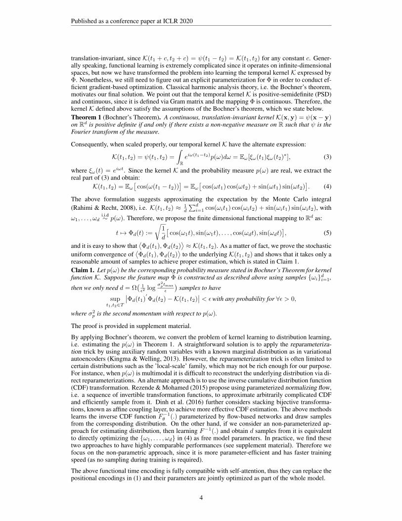
Figure 1: Visual illustration for several complications from the temporal graphs. (A). The gen-eration process of a temporal graph and its snapshots. It is obvious that the static graphs in thesnapshots only reflect partial temporal information. (B). The final state of the temporal graph whenprojected to the time-independent 2-D plane. Other than the missing temporal information, themulti-edge situation arises as well. (C). When predicting the link between node A and C at timet3, the message-passing paths should be subject to temporal contraints. The solid lines give theappropriate directions, and the dashed lines violates the temporal constraints.

temporal constraints on neighborhood aggregation methods. Thirdly, node features and topolog-ical structures can exhibit temporal patterns. For example, node interactions that took place longago may have less impact on the current topological structure and thus the node embeddings. Also,some nodes may possess features that allows them having more regular or recurrent interactionswith others. We provide sketched plots for visual illustration in Figure 1.

Similar to its non-temporal counterparts, in the real-world applications, models for representa-tion learning on temporal graphs should be able to quickly generate embeddings whenever re-quired, in an inductive fashion. GraphSAGE (Hamilton et al., 2017a) and graph attention network(GAT ) (Velickovic et al., 2017) are capable of inductively generating embeddings for unseen nodesbased on their features, however, they do not consider the temporal factors. Most of the temporalgraph embedding methods can only handle transductive tasks, since they require re-training or thecomputationally-expensive gradient calculations to infer embeddings for unseen nodes or node em-beddings for a new timepoint. In this work, we aim at developing an architecture to inductively learnrepresentations for temporal graphs such that the time-aware embeddings (for unseen and observednodes) can be obtained via a single network forward pass. The key to our approach is the combi-nation of the self-attention mechanism (Vaswani et al., 2017) and a novel functional time encodingtechnique derived from the Bochner’s theorem from classical harmonic analysis (Loomis, 2013).

The motivation for adapting self-attention to inductive representation learning on temporal graphs isto identify and capture relevant pieces of the temporal neighborhood information. Both graph con-volutional network (GCN ) (Kipf & Welling, 2016a) and GAT are implicitly or explicitly assigningdifferent weights to neighboring nodes (Velickovic et al., 2017) when aggregating node features. Theself-attention mechanism was initially designed to recognize the relevant parts of input sequence innatural language processing. As a discrete-event sequence learning method, self-attention outputs avector representation of the input sequence as a weighted sum of individual entry embeddings. Self-attention enjoys several advantages such as parallelized computation and interpretability (Vaswaniet al., 2017). Since it captures sequential information only through the positional encoding, tem-poral features can not be handled. Therefore, we are motivated to replace positional encoding withsome vector representation of time. Since time is a continuous variable, the mapping from the timedomain to vector space has to be functional. We gain insights from harmonic analysis and proposea theoretical-grounded functional time encoding approach that is compatible with the self-attentionmechanism. The temporal signals are then modelled by the interactions between the functional timeencoding and nodes features as well as the graph topological structures.

To evaluate our approach, we consider future link prediction on the observed nodes as transductivelearning task, and on the unseen nodes as inductive learning task. We also examine the dynamic nodeclassification task using node embeddings (temporal versus non-temporal) as features to demonstratethe usefulness of our functional time encoding. We carry out extensive ablation studies and sensi-tivity analysis to show the effectiveness of the proposed functional time encoding and TGAT -layer.

2


2 RELATED WORK

Graph representation learning. Spectral graph embedding models operate on the graph spectraldomain by approximating, projecting or expanding the graph Laplacian (Kipf & Welling, 2016a;Henaff et al., 2015; Defferrard et al., 2016). Since their training and inference are conditioned onthe specific graph spectrum, they are not directly extendable to temporal graphs. Non-spectral ap-proaches, such as GAT, GraphSAGE and MoNET, (Monti et al., 2017) rely on the localized neigh-bourhood aggregations and thus are not restricted to the training graph. GraphSAGE and GAT alsohave the flexibility to handle evolving graphs inductively. To extend classical graph representationlearning approaches to the temporal domain, several attempts have been done by cropping the tem-poral graph into a sequence of graph snapshots (Li et al., 2018; Goyal et al., 2018; Rahman et al.,2018; Xu et al., 2019b), and some others work with temporally persistent node (edges) (Trivedi et al.,2018; Ma et al., 2018). Nguyen et al. (2018) proposes a node embedding method based on temporalrandom walk and reported state-of-the-art performances. However, their approach only generatesembeddings for the final state of temporal graph and can not directly apply to the inductive setting.

Self-attention mechanism. Self-attention mechanisms often have two components: the embeddinglayer and the attention layer. The embedding layer takes an ordered entity sequence as input. Self-attention uses the positional encoding, i.e. each position k is equipped with a vector pk (fixed orlearnt) which is shared for all sequences. For the entity sequence e = (e1, . . . , el), the embeddinglayer takes the sum or concatenation of entity embeddings (or features) (z ∈ Rd) and their positionalencodings as input:

Ze =[ze1 + p1, . . . , ze1 + pl

]ᵀ ∈ Rl×d, or Ze =[ze1 ||p1, . . . , ze1 ||pl

]ᵀ ∈ Rl×(d+dpos). (1)

where || denotes concatenation operation and dpos is the dimension for positional encoding. Self-attention layers can be constructed using the scaled dot-product attention, which is defined as:

Attn(Q,K,V

)= softmax

(QKᵀ

√d

)V, (2)

where Q denotes the ’queries’, K the ’keys’ and V the ’values’. In Vaswani et al. (2017), they aretreated as projections of the output Ze: Q = ZeWQ, K = ZeWK , V = ZeWV , where WQ,WK and WV are the projection matrices. Since each row of Q, K and V represents an entity, thedot-product attention takes a weighted sum of the entity ’values’ in V where the weights are givenby the interactions of entity ’query-key’ pairs. The hidden representation for the entity sequenceunder the dot-product attention is then given by he = Attn(Q,K,V).

3 TEMPORAL GRAPH ATTENTION NETWORK ARCHITECTURE

We first derive the mapping from time domain to the continuous differentiable functional domainas the functional time encoding such that resulting formulation is compatible with self-attentionmechanism as well as the backpropagation-based optimization frameworks. The same idea wasexplored in a concurrent work (Xu et al., 2019a). We then present the temporal graph attention layerand show how it can be naturally extended to incorporate the edge features.

3.1 FUNCTIONAL TIME ENCODING

Recall that our starting point is to obtain a continuous functional mapping Φ : T → RdT fromtime domain to the dT -dimensional vector space to replace the positional encoding in (1). Withoutloss of generality, we assume that the time domain can be represented by the interval starting fromorigin: T = [0, tmax], where tmax is determined by the observed data. For the inner-product self-attention in (2), often the ’key’ and ’query’ matrices (K, Q) are given by identity or linear projectionof Ze defined in (1), leading to terms that only involve inner-products between positional (time)encodings. Consider two time points t1, t2 and inner product between their functional encodings⟨Φ(t1),Φ(t2)

⟩. Usually, the relative timespan, rather than the absolute value of time, reveals critical

temporal information. Therefore, we are more interested in learning patterns related to the timespanof |t2−t1|, which should be ideally expressed by

⟨Φ(t1),Φ(t2)

⟩to be compatible with self-attention.

Formally, we define the temporal kernel K : T × T → R with K(t1, t2) :=⟨Φ(t1),Φ(t2)

⟩and

K(t1, t2) = ψ(t1 − t2), ∀t1, t2 ∈ T for some ψ : [−tmax, tmax] → R. The temporal kernel is then

3


translation-invariant, since K(t1 + c, t2 + c) = ψ(t1 − t2) = K(t1, t2) for any constant c. Gener-ally speaking, functional learning is extremely complicated since it operates on infinite-dimensionalspaces, but now we have transformed the problem into learning the temporal kernel K expressed byΦ. Nonetheless, we still need to figure out an explicit parameterization for Φ in order to conduct ef-ficient gradient-based optimization. Classical harmonic analysis theory, i.e. the Bochner’s theorem,motivates our final solution. We point out that the temporal kernel K is positive-semidefinite (PSD)and continuous, since it is defined via Gram matrix and the mapping Φ is continuous. Therefore, thekernel K defined above satisfy the assumptions of the Bochner’s theorem, which we state below.Theorem 1 (Bochner’s Theorem). A continuous, translation-invariant kernel K(x,y) = ψ(x− y)on Rd is positive definite if and only if there exists a non-negative measure on R such that ψ is theFourier transform of the measure.

Consequently, when scaled properly, our temporal kernel K have the alternate expression:

K(t1, t2) = ψ(t1, t2) =

∫Reiω(t1−t2)p(ω)dω = Eω[ξω(t1)ξω(t2)∗], (3)

where ξω(t) = eiωt. Since the kernel K and the probability measure p(ω) are real, we extract thereal part of (3) and obtain:

K(t1, t2) = Eω[

cos(ω(t1 − t2))]

= Eω[

cos(ωt1) cos(ωt2) + sin(ωt1) sin(ωt2)]. (4)

The above formulation suggests approximating the expectation by the Monte Carlo integral(Rahimi & Recht, 2008), i.e. K(t1, t2) ≈ 1

d

∑di=1 cos(ωit1) cos(ωit2) + sin(ωit1) sin(ωit2), with

ω1, . . . , ωdi.i.d∼ p(ω). Therefore, we propose the finite dimensional functional mapping to Rd as:

t 7→ Φd(t) :=

√1

d

[cos(ω1t), sin(ω1t), . . . , cos(ωdt), sin(ωdt)

], (5)

and it is easy to show that⟨Φd(t1),Φd(t2)

⟩≈ K(t1, t2). As a matter of fact, we prove the stochastic

uniform convergence of⟨Φd(t1),Φd(t2)

⟩to the underlying K(t1, t2) and shows that it takes only a

reasonable amount of samples to achieve proper estimation, which is stated in Claim 1.Claim 1. Let p(ω) be the corresponding probability measure stated in Bochner’s Theorem for kernelfunction K. Suppose the feature map Φ is constructed as described above using samples ωidi=1,

then we only need d = Ω(

1ε2 log

σ2ptmax

ε

)samples to have

supt1,t2∈T

∣∣Φd(t1)′Φd(t2)−K(t1, t2)

∣∣ < εwith any probability for ∀ε > 0,

where σ2p is the second momentum with respect to p(ω).

The proof is provided in supplement material.

By applying Bochner’s theorem, we convert the problem of kernel learning to distribution learning,i.e. estimating the p(ω) in Theorem 1. A straightforward solution is to apply the reparameteriza-tion trick by using auxiliary random variables with a known marginal distribution as in variationalautoencoders (Kingma & Welling, 2013). However, the reparameterization trick is often limited tocertain distributions such as the ’local-scale’ family, which may not be rich enough for our purpose.For instance, when p(ω) is multimodal it is difficult to reconstruct the underlying distribution via di-rect reparameterizations. An alternate approach is to use the inverse cumulative distribution function(CDF) transformation. Rezende & Mohamed (2015) propose using parameterized normalizing flow,i.e. a sequence of invertible transformation functions, to approximate arbitrarily complicated CDFand efficiently sample from it. Dinh et al. (2016) further considers stacking bijective transforma-tions, known as affine coupling layer, to achieve more effective CDF estimation. The above methodslearns the inverse CDF function F−1

θ (.) parameterized by flow-based networks and draw samplesfrom the corresponding distribution. On the other hand, if we consider an non-parameterized ap-proach for estimating distribution, then learning F−1(.) and obtain d samples from it is equivalentto directly optimizing the ω1, . . . , ωd in (4) as free model parameters. In practice, we find thesetwo approaches to have highly comparable performances (see supplement material). Therefore wefocus on the non-parametric approach, since it is more parameter-efficient and has faster trainingspeed (as no sampling during training is required).

The above functional time encoding is fully compatible with self-attention, thus they can replace thepositional encodings in (1) and their parameters are jointly optimized as part of the whole model.

4


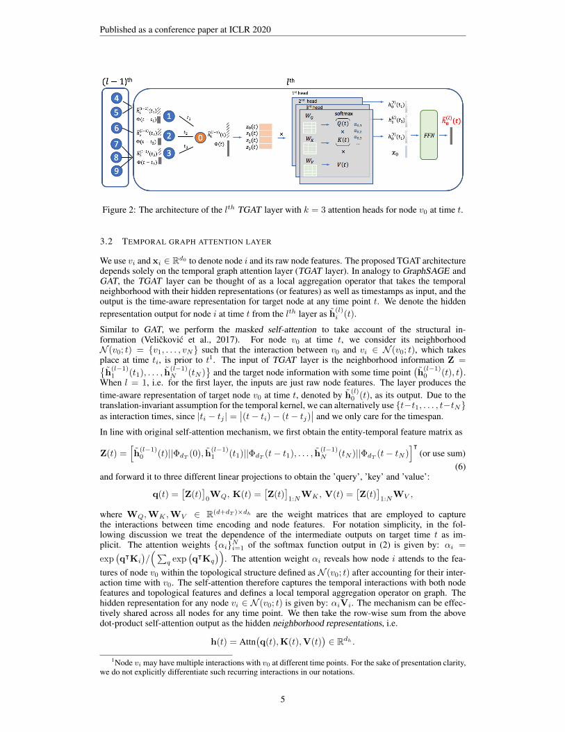
Figure 2: The architecture of the lth TGAT layer with k = 3 attention heads for node v0 at time t.

3.2 TEMPORAL GRAPH ATTENTION LAYER

We use vi and xi ∈ Rd0 to denote node i and its raw node features. The proposed TGAT architecturedepends solely on the temporal graph attention layer (TGAT layer). In analogy to GraphSAGE andGAT, the TGAT layer can be thought of as a local aggregation operator that takes the temporalneighborhood with their hidden representations (or features) as well as timestamps as input, and theoutput is the time-aware representation for target node at any time point t. We denote the hiddenrepresentation output for node i at time t from the lth layer as h(l)

i (t).

Similar to GAT, we perform the masked self-attention to take account of the structural in-formation (Velickovic et al., 2017). For node v0 at time t, we consider its neighborhoodN (v0; t) = v1, . . . , vN such that the interaction between v0 and vi ∈ N (v0; t), which takesplace at time ti, is prior to t1. The input of TGAT layer is the neighborhood information Z =h

(l−1)1 (t1), . . . , h

(l−1)N (tN )

and the target node information with some time point

(h

(l−1)0 (t), t

).

When l = 1, i.e. for the first layer, the inputs are just raw node features. The layer produces thetime-aware representation of target node v0 at time t, denoted by h

(l)0 (t), as its output. Due to the

translation-invariant assumption for the temporal kernel, we can alternatively use t−t1, . . . , t−tNas interaction times, since |ti − tj | =

∣∣(t− ti)− (t− tj)∣∣ and we only care for the timespan.

In line with original self-attention mechanism, we first obtain the entity-temporal feature matrix as

Z(t) =[h

(l−1)0 (t)||ΦdT (0), h

(l−1)1 (t1)||ΦdT (t− t1), . . . , h

(l−1)N (tN )||ΦdT (t− tN )

]ᵀ(or use sum)

(6)and forward it to three different linear projections to obtain the ’query’, ’key’ and ’value’:

q(t) =[Z(t)

]0WQ, K(t) =

[Z(t)

]1:N

WK , V(t) =[Z(t)

]1:N

WV ,

where WQ,WK ,WV ∈ R(d+dT )×dh are the weight matrices that are employed to capturethe interactions between time encoding and node features. For notation simplicity, in the fol-lowing discussion we treat the dependence of the intermediate outputs on target time t as im-plicit. The attention weights αiNi=1 of the softmax function output in (2) is given by: αi =

exp(qᵀKi

)/(∑

q exp(qᵀKq

)). The attention weight αi reveals how node i attends to the fea-

tures of node v0 within the topological structure defined as N (v0; t) after accounting for their inter-action time with v0. The self-attention therefore captures the temporal interactions with both nodefeatures and topological features and defines a local temporal aggregation operator on graph. Thehidden representation for any node vi ∈ N (v0; t) is given by: αiVi. The mechanism can be effec-tively shared across all nodes for any time point. We then take the row-wise sum from the abovedot-product self-attention output as the hidden neighborhood representations, i.e.

h(t) = Attn(q(t),K(t),V(t)

)∈ Rdh .

1Node vi may have multiple interactions with v0 at different time points. For the sake of presentation clarity,we do not explicitly differentiate such recurring interactions in our notations.

5


To combine neighbourhood representation with the target node features, we adopt the same practicefrom GraphSAGE and concatenate the neighbourhood representation with the target node’s fea-ture vector z0. We then pass it to a feed-forward neural network to capture non-linear interactionsbetween the features as in (Vaswani et al., 2017):

h(l)0 (t) = FFN

(h(t)||x0

)≡ ReLU

([h(t)||x0]W

(l)0 + b

(l)0

)W

(l)1 + b

(l)1 ,

W(l)0 ∈ R(dh+d0)×df ,W

(l)1 ∈ Rdf×d,b(l)

0 ∈ Rdf ,b(l)1 ∈ Rd,

where h(l)0 (t) ∈ Rd is the final output representing the time-aware node embedding at time t for

the target node. Therefore, the TGAT layer can be implemented for node classification task usingthe semi-supervised learning framework proposed in Kipf & Welling (2016a) as well as the linkprediction task with the encoder-decoder framework summarized by Hamilton et al. (2017b).

Velickovic et al. (2017) suggests that using multi-head attention improves performances and stabi-lizes training for GAT. For generalization purposes, we also show that the proposed TGAT layer canbe easily extended to the multi-head setting. Consider the dot-product self-attention outputs from atotal of k different heads, i.e. h(i) ≡ Attn(i)

(q(t),K(t),V(t)

), i = 1, . . . , k. We first concatenate

the k neighborhood representations into a combined vector and then carry out the same procedure:

h(l)0 (t) = FFN

(h(1)(t)|| . . . ||h(k)(t)||x0

).

Just like GraphSAGE, a single TGAT layer aggregates the localized one-hop neighborhood, and bystacking L TGAT layers the aggregation extends to L hops. Similar to GAT, out approach does notrestrict the size of neighborhood. We provide a graphical illustration of our TGAT layer in Figure 2.

3.3 EXTENSION TO INCORPORATE EDGE FEATURES

We show that the TGAT layer can be naturally extended to handle edge features in a message-passing fashion. Simonovsky & Komodakis (2017) and Wang et al. (2018b) modify classicalspectral-based graph convolutional networks to incorporate edge features. Battaglia et al. (2018)propose general graph neural network frameworks where edges features can be processed. For tem-poral graphs, we consider the general setting where each dynamic edge is associated with a featurevector, i.e. the interaction between vi and vj at time t induces the feature vector xi,j(t). To propagateedge features during the TGAT aggregation, we simply extend the Z(t) in (6) to:

Z(t) =[. . . , h

(l−1)i (ti)||x0,i(ti)||ΦdT (t− ti), . . .

](or use summation), (7)

such that the edge information is propagated to the target node’s hidden representation, and thenpassed on to the next layer (if exists). The remaining structures stay the same as in Section 3.2.

3.4 TEMPORAL SUB-GRAPH BATCHING

Stacking L TGAT layers is equivalent to aggregate over the L-hop neighborhood. For each L-hopsub-graph that is constructed during the batch-wise training, all message passing directions mustbe aligned with the observed chronological orders. Unlike the non-temporal setting where eachedge appears only once, in temporal graphs two node can have multiple interactions at differenttime points. Whether or not to allow loops that involve the target node should be judged case-by-case. Sampling from neighborhood, or known as neighborhood dropout, may speed up and stabilizemodel training. For temporal graphs, neighborhood dropout can be carried uniformly or weightedby the inverse timespan such that more recent interactions has higher probability of being sampled.

3.5 COMPARISONS TO RELATED WORK

The functional time encoding technique and TGAT layer introduced in Section 3.1 and 3.2 solvesseveral critical challenges, and the TGAT network intrinsically connects to several prior methods.

• Instead of cropping temporal graphs into a sequence of snapshots or constructing time-constraint random walks, which inspired most of the current temporal graph embeddingmethods, we directly learn the functional representation of time. The proposed approach is

6


motivated by and thus fully compatible with the well-established self-attention mechanism.Also, to the best of our knowledge, no previous work has discussed the temporal-featureinteractions for temporal graphs, which is also considered in our approach.

• The TGAT layer is computationally efficient compared with RNN-based models, since themasked self-attention operation is parallelizable, as suggested by Vaswani et al. (2017). Theper-batch time complexity of the TGAT layer with k heads and l layers can be expressed asO((kN)l

)where N is the average neighborhood size, which is comparable to GAT. When

using multi-head attention, the computation for each head can be parallelized as well.

• The inference with TGAT is entirely inductive. With an explicit functional expression h(t)for each node, the time-aware node embeddings can be easily inferred for any timestampvia a single network forward pass. Similarity, whenever the graph is updated, the embed-dings for both unseen and observed nodes can be quickly inferred in an inductive fashionsimilar to that of GraphSAGE, and the computations can be parallelized across all nodes.

• GraphSAGE with mean pooling (Hamilton et al., 2017a) can be interpreted as a specialcase of the proposed method, where the temporal neighborhood is aggregated with equalattention coefficients. GAT is like the time-agnostic version of our approach but with adifferent formulation for self-attention, as they refer to the work of Bahdanau et al. (2014).We discuss the differences in detail in the Appendix. It is also straightforward to show ourconnections with the menory networks (Sukhbaatar et al., 2015) by thinking of the temporalneighborhoods as memory. The techniques developed in our work may also help adaptingGAT and GraphSAGE to temporal settings as we show in our experiments.

4 EXPERIMENT AND RESULTS

We test the performance of the proposed method against a variety of strong baselines (adapted fortemporal settings when possible) and competing approaches, for both the inductive and transductivetasks on two benchmark and one large-scale industrial dataset.

4.1 DATASETS

Real-world temporal graphs consist of time-sensitive node interactions, evolving node labels as wellas new nodes and edges. We choose the following datasets which contain all scenarios.

Reddit dataset.2 We use the data from active users and their posts under subreddits, leading to atemporal graph with 11,000 nodes,∼700,000 temporal edges and dynamic labels indicating whethera user is banned from posting. The user posts are transformed into edge feature vectors.

Wikipedia dataset.3 We use the data from top edited pages and active users, yielding a temporalgraph ∼9,300 nodes and around 160,000 temporal edges. Dynamic labels indicate if users aretemporarily banned from editing. The user edits are also treated as edge features.

Industrial dataset. We choose 70,000 popular products and 100,000 active customers as nodes fromthe online grocery shopping website4 and use the customer-product purchase as temporal edges (∼2million). The customers are tagged with labels indicating if they have a recent interest in dietaryproducts. Product features are given by the pre-trained product embeddings (Xu et al., 2020).

We do the chronological train-validation-test split with 70%-15%-15% according to node interactiontimestamps. The dataset and preprocessing details are provided in the supplement material.

4.2 TRANSDUCTIVE AND INDUCTIVE LEARNING TASKS

Since the majority of temporal information is reflected via the timely interactions among nodes, wechoose to use a more revealing link prediction setup for training. Node classification is then treatedas the downstream task using the obtained time-aware node embeddings as input.

2http://snap.stanford.edu/jodie/reddit.csv3http://snap.stanford.edu/jodie/wikipedia.csv4https://grocery.walmart.com/

7


Dataset Reddit Wikipedia IndustrialMetric Accuracy AP Accuracy AP Accuracy APGAE 74.31 (0.5) 93.23 (0.3) 72.85 (0.7) 91.44 (0.1) 68.92 (0.3) 81.15 (0.2)

VAGE 74.19 (0.4) 92.92 (0.2) 78.01 (0.3) 91.34 (0.3) 67.81 (0.4) 80.87 (0.3)DeepWalk 71.43 (0.6) 83.10 (0.5) 76.67 (0.5) 90.71 (0.6) 65.87 (0.3) 80.93 (0.2)Node2vec 72.53 (0.4) 84.58 (0.5) 78.09 (0.4) 91.48 (0.3) 66.64 (0.3) 81.39 (0.3)CTDNE 73.76 (0.5) 91.41 (0.3) 79.42 (0.4) 92.17 (0.5) 67.81 (0.3) 80.95 (0.5)

GAT 92.14 (0.2) 97.33 (0.2) 87.34 (0.3) 94.73 (0.2) 69.58 (0.4) 81.51 (0.2)GAT+T 92.47 (0.2) 97.62 (0.2) 87.57 (0.2) 95.14 (0.4) 70.15 (0.3) 82.66 (0.4)

GraphSAGE 92.31(0.2) 97.65 (0.2) 85.93 (0.3) 93.56 (0.3) 70.19 (0.2) 83.27 (0.3)GraphSAGE+T 92.58 (0.2) 97.89 (0.3) 86.31 (0.3) 93.72 (0.3) 71.84 (0.3) 84.95 (0.)

Const-TGAT 91.39 (0.2) 97.86 (0.2) 86.03 (0.4) 93.50 (0.3) 68.52 (0.2) 81.91 (0.3)TGAT 92.92 (0.3) 98.12 (0.2) 88.14 (0.2) 95.34 (0.1) 73.28 (0.2) 86.32 (0.1)

Table 1: Transductive learning task results for predicting future edges of nodes that have been ob-served in training data. All results are converted to percentage by multiplying by 100, and the stan-dard deviations computed over ten runs (in parenthesis). The best and second-best results in eachcolumn are highlighted in bold font and underlined. GraphSAGE is short for GraphSAGE -LSTM.

Dataset Reddit Wikipedia IndustrialMetric Accuracy AP Accuracy AP Accuracy APGAT 89.86 (0.2) 95.37 (0.3) 82.36 (0.3) 91.27 (0.4) 68.28 (0.2) 79.93 (0.3)

GAT+T 90.44 (0.3) 96.31 (0.3) 84.82 (0.3) 93.57 (0.3) 69.51 (0.3) 81.68 (0.3)GraphSAGE 89.43 (0.1) 96.27 (0.2) 82.43 (0.3) 91.09 (0.3) 67.49 (0.2) 80.54 (0.3)

GraphSAGE+T 90.07 (0.2) 95.83 (0.2) 84.03 (0.4) 92.37 (0.5) 69.66 (0.3) 82.74 (0.3)Const-TGAT 88.28 (0.3) 94.12 (0.2) 83.60 (0.4) 91.93 (0.3) 65.87 (0.3) 77.03 (0.4)

TGAT 90.73 (0.2) 96.62 (0.3) 85.35 (0.2) 93.99 (0.3) 72.08 (0.3) 84.99 (0.2)

Table 2: Inductive learning task results for predicting future edges of unseen nodes.

Transductive task examines embeddings of the nodes that have been observed in training, via thefuture link prediction task and the node classification. To avoid violating temporal constraints, wepredict the links that strictly take place posterior to all observations in the training data.

Inductive task examines the inductive learning capability using the inferred representations of un-seen nodes, by predicting the future links between unseen nodes and classify them based on theirinferred embedding dynamically. We point out that it suffices to only consider the future sub-graphfor unseen nodes since they are equivalent to new graphs under the non-temporal setting.

As for the evaluation metrics, in the link prediction tasks, we first sample an equal amount of nega-tive node pairs to the positive links and then compute the average precision (AP) and classificationaccuracy. In the downstream node classification tasks, due to the label imbalance in the datasets,we employ the area under the ROC curve (AUC).

4.3 BASELINES

Transductive task: for link prediction of observed nodes, we choose the compare our approachwith the state-of-the-art graph embedding methods: GAE and VGAE (Kipf & Welling, 2016b). Forcomplete comparisons, we also include the skip-gram-based node2vec (Grover & Leskovec, 2016)as well as the spectral-based DeepWalk model (Perozzi et al., 2014), using the same inner-productdecoder as GAE for link prediction. The CDTNE model based on the temporal random walk hasbeen reported with superior performance on transductive learning tasks (Nguyen et al., 2018), so weinclude CDTNE as the representative for temporal graph embedding approaches.

Inductive task: few approaches are capable of managing inductive learning on graphs even in thenon-temporal setting. As a consequence, we choose GraphSAGE and GAT as baselines after adapt-ing them to the temporal setting. In particular, we equip them with the same temporal sub-graphbatching describe in Section 3.4 to maximize their usage on temporal information. Also, we im-plement the extended version for the baselines to include edge features in the same way as ours(in Section 3.3). We experiment on different aggregation functions for GraphSAGE, i.e. Graph-

8


SAGE -mean, GraphSAGE -pool and GraphSAGE -LSTM. In accordance with the original work ofHamilton et al. (2017a), GraphSAGE -LSTM gives the best validation performance among the threeapproaches, which is reasonable under temporal setting since LSTM aggregation takes account ofthe sequential information. Therefore we report the results of GraphSAGE -LSTM.

In addition to the above baselines, we implement a version of TGAT with all temporal attentionweights set to equal value (Const-TGAT ). Finally, to show that the superiority of our approach owesto both the time encoding and the network architecture, we experiment with the enhanced GATand GraphSAGE -mean by concatenating the proposed time encoding to the original features duringtemporal aggregations (GAT+T and GraphSAGE+T ).

Figure 3: Results of node classificationtask in the ablation study.

Dataset Reddit Wikipedia IndustrialGAE 58.39 (0.5) 74.85 (0.6) 76.59 (0.3)

VGAE 57.98 (0.6) 73.67 (0.8) 75.38 (0.4)CTDNE 59.43 (0.6) 75.89 (0.5) 78.36 (0.5)

GAT 64.52 (0.5) 82.34 (0.8) 87.43 (0.4)GAT+T 64.76 (0.6) 82.95 (0.7) 88.24 (0.5)

GraphSAGE 61.24 (0.6) 82.42 (0.7) 88.28 (0.3)GraphSAGE+T 62.31 (0.7) 82.87 (0.6) 89.81 (0.3)

Const-TGAT 60.97 (0.5) 75.18 (0.7) 82.59 (0.6)TGAT 65.56 (0.7) 83.69 (0.7) 92.31 (0.3)

Table 3: Dynamic node classification task results, where thereported metric is the AUC.

4.4 EXPERIMENT SETUP

We use the time-sensitive link prediction loss function for training the l-layer TGAT network:

` =∑

(vi,vj ,tij)∈E

− log(σ(− hli(tij)

ᵀhlj(tij)))−Q.Evq∼Pn(v) log

(σ(hli(tij)

ᵀhlq(tij))), (8)

where the summation is over the observed edges on vi and vj that interact at time tij , and σ(.) is thesigmoid function, Q is the number of negative samples and Pn(v) is the negative sampling distri-bution over the node space. As for tuning hyper-parameters, we fix the node embedding dimensionand the time encoding dimension to be the original feature dimension for simplicity, and then selectthe number of TGAT layers from 1,2,3, the number of attention heads from 1,2,3,4,5, accord-ing to the link prediction AP score in the validation dataset. Although our method does not putrestriction on the neighborhood size during aggregations, to speed up training, specially when usingthe multi-hop aggregations, we use neighborhood dropout (selected among p =0.1, 0.3, 0.5) withthe uniform sampling. During training, we use 0.0001 as learning rate for Reddit and Wikipediadataset and 0.001 for the industrial dataset, with Glorot initialization and the Adam SGD optimizer.We do not experiment on applying regularization since our approach is parameter-efficient and onlyrequires Ω

((d + dT )dh + (dh + d0)df + dfd

)parameters for each attention head, which is inde-

pendent of the graph and neighborhood size. Using two TGAT layers and two attention heads withdropout rate as 0.1 give the best validation performance. For inference, we inductively compute theembeddings for both the unseen and observed nodes at each time point that the graph evolves, orwhen the node labels are updated. We then use these embeddings as features for the future linkprediction and dynamic node classifications with multilayer perceptron.

We further conduct ablation study to demonstrate the effectiveness of the proposed functional timeencoding approach. We experiment on abandoning time encoding or replacing it with the originalpositional encoding (both fixed and learnt). We also compare the uniform neighborhood dropout tosampling with inverse timespan (where the recent edges are more likely to be sampled), which isprovided in supplement material along with other implementation details and setups for baselines.

4.5 RESULTS

The results in Table 1 and Table 2 demonstrates the state-of-the-art performances of our approach onboth transductive and inductive learning tasks. In the inductive learning task, our TGAT network sig-nificantly improves upon the the upgraded GraphSAGE -LSTM and GAT in accuracy and average

9


precision by at least 5 % for both metrics, and in the transductive learning task TGAT consistentlyoutperforms all baselines across datasets. While GAT+T and GraphSAGE+T slightly outperformor tie with GAT and GraphSAGE -LSTM, they are nevertheless outperformed by our approach. Onone hand, the results suggest that the time encoding have potential to extend non-temporal graphrepresentation learning methods to temporal settings. On the other, we note that the time encodingstill works the best with our network architecture which is designed for temporal graphs. Over-all, the results demonstrate the superiority of our approach in learning representations on temporalgraphs over prior models. We also see the benefits from assigning temporal attention weights toneighboring nodes, where GAT significantly outperforms the Const-TGAT in all three tasks. Thedynamic node classification outcome (in Table 3) further suggests the usefulness of our time-awarenode embeddings for downstream tasks as they surpass all the baselines. The ablation study resultsof Figure 3 successfully reveals the effectiveness of the proposed functional time encoding approachin capturing temporal signals as it outperforms the positional encoding counterparts.

4.6 ATTENTION ANALYSIS

To shed some insights into the temporal signals captured by the proposed TGAT, we analyze thepattern of the attention weights αij(t) as functions of both time t and node pairs (i, j) in theinference stage. Firstly, we analyze how the attention weights change with respect to the timespansof previous interactions, by plotting the attention weights

αjq(tij)|q ∈ N (vj ; tij)

∪αik(tij)|k ∈

N (vi; tij)

against the timespans tij−tjq∪tij−tikwhen predicting the link for (vi, vj , tij) ∈ E(Figure 4a). This gives us an empirical estimation on the α(∆t), where a smaller ∆t means a morerecent interaction. Secondly, we analyze how the topological structures affect the attention weightsas time elapses. Specifically, we focus on the topological structure of the recurring neighbours, byfinding out what attention weights the model put on the neighbouring nodes with different number ofreoccurrences. Since the functional forms of all αij(.) are fixed after training, we are able to feedin different target time t and then record their value on neighbouring nodes with different numberof occurrences (Figure 4b). From Figure 4a we observe that TGAT captures the pattern of havingless attention on more distant interactions in all three datasets. In Figure 4b, it is obvious that whenpredicting a more future interaction, TGAT will consider neighbouring nodes who have a highernumber of occurrences of more importance. The patterns of the attention weights are meaningful,since the more recent and repeated actions often have larger influence on users’ future interests.

Figure 4: Attention weight analysis. We apply the Loess smoothing method for visualization.

5 CONCLUSION AND FUTURE WORK

We introduce a novel time-aware graph attention network for inductive representation learning ontemporal graphs. We adapt the self-attention mechanism to handle the continuous time by proposinga theoretically-grounded functional time encoding. Theoretical and experimental analysis demon-strate the effectiveness of our approach for capturing temporal-feature signals in terms of both nodeand topological features on temporal graphs. Self-attention mechanism often provides useful modelinterpretations (Vaswani et al., 2017), which is an important direction of our future work. Develop-ing tools to visualize the evolving graph dynamics and temporal representations efficiently is anotherimportant direction for both research and application. Also, the functional time encoding techniquehas huge potential for adapting other deep learning methods to the temporal graph domain.

10


REFERENCES

Dzmitry Bahdanau, Kyunghyun Cho, and Yoshua Bengio. Neural machine translation by jointlylearning to align and translate. arXiv preprint arXiv:1409.0473, 2014.

Peter W Battaglia, Jessica B Hamrick, Victor Bapst, Alvaro Sanchez-Gonzalez, Vinicius Zambaldi,Mateusz Malinowski, Andrea Tacchetti, David Raposo, Adam Santoro, Ryan Faulkner, et al.Relational inductive biases, deep learning, and graph networks. arXiv preprint arXiv:1806.01261,2018.

Michael Defferrard, Xavier Bresson, and Pierre Vandergheynst. Convolutional neural networks ongraphs with fast localized spectral filtering. In Advances in neural information processing systems,pp. 3844–3852, 2016.

Laurent Dinh, Jascha Sohl-Dickstein, and Samy Bengio. Density estimation using real nvp. arXivpreprint arXiv:1605.08803, 2016.

Matthias Fey and Jan E. Lenssen. Fast graph representation learning with PyTorch Geometric. InICLR Workshop on Representation Learning on Graphs and Manifolds, 2019.

Palash Goyal, Nitin Kamra, Xinran He, and Yan Liu. Dyngem: Deep embedding method for dy-namic graphs. arXiv preprint arXiv:1805.11273, 2018.

Aditya Grover and Jure Leskovec. node2vec: Scalable feature learning for networks. In Proceedingsof the 22nd ACM SIGKDD international conference on Knowledge discovery and data mining,pp. 855–864. ACM, 2016.

Will Hamilton, Zhitao Ying, and Jure Leskovec. Inductive representation learning on large graphs.In Advances in Neural Information Processing Systems, pp. 1024–1034, 2017a.

William L Hamilton, Rex Ying, and Jure Leskovec. Representation learning on graphs: Methodsand applications. arXiv preprint arXiv:1709.05584, 2017b.

Mikael Henaff, Joan Bruna, and Yann LeCun. Deep convolutional networks on graph-structureddata. arXiv preprint arXiv:1506.05163, 2015.

Diederik P Kingma and Max Welling. Auto-encoding variational bayes. arXiv preprintarXiv:1312.6114, 2013.

Thomas N Kipf and Max Welling. Semi-supervised classification with graph convolutional net-works. arXiv preprint arXiv:1609.02907, 2016a.

Thomas N Kipf and Max Welling. Variational graph auto-encoders. arXiv preprintarXiv:1611.07308, 2016b.

Taisong Li, Jiawei Zhang, S Yu Philip, Yan Zhang, and Yonghong Yan. Deep dynamic networkembedding for link prediction. IEEE Access, 6:29219–29230, 2018.

Lynn H Loomis. Introduction to abstract harmonic analysis. Courier Corporation, 2013.

Yao Ma, Ziyi Guo, Eric Zhao Zhaochun Ren, and Dawei Yin Jiliang Tang. Streaming graph neuralnetworks. arXiv preprint arXiv:1810.10627, 2018.

Federico Monti, Davide Boscaini, Jonathan Masci, Emanuele Rodola, Jan Svoboda, and Michael MBronstein. Geometric deep learning on graphs and manifolds using mixture model cnns. InProceedings of the IEEE Conference on Computer Vision and Pattern Recognition, pp. 5115–5124, 2017.

Giang Hoang Nguyen, John Boaz Lee, Ryan A Rossi, Nesreen K Ahmed, Eunyee Koh, andSungchul Kim. Continuous-time dynamic network embeddings. In Companion Proceedings ofthe The Web Conference 2018, pp. 969–976. International World Wide Web Conferences SteeringCommittee, 2018.

James W Pennebaker, Martha E Francis, and Roger J Booth. Linguistic inquiry and word count:Liwc 2001. Mahway: Lawrence Erlbaum Associates, 71(2001):2001, 2001.

11


Bryan Perozzi, Rami Al-Rfou, and Steven Skiena. Deepwalk: Online learning of social repre-sentations. In Proceedings of the 20th ACM SIGKDD international conference on Knowledgediscovery and data mining, pp. 701–710. ACM, 2014.

Ali Rahimi and Benjamin Recht. Random features for large-scale kernel machines. In Advances inneural information processing systems, pp. 1177–1184, 2008.

Mahmudur Rahman, Tanay Kumar Saha, Mohammad Al Hasan, Kevin S Xu, and Chandan K Reddy.Dylink2vec: Effective feature representation for link prediction in dynamic networks. arXivpreprint arXiv:1804.05755, 2018.

Danilo Jimenez Rezende and Shakir Mohamed. Variational inference with normalizing flows. arXivpreprint arXiv:1505.05770, 2015.

Martin Simonovsky and Nikos Komodakis. Dynamic edge-conditioned filters in convolutional neu-ral networks on graphs. In Proceedings of the IEEE conference on computer vision and patternrecognition, pp. 3693–3702, 2017.

Sainbayar Sukhbaatar, Jason Weston, Rob Fergus, et al. End-to-end memory networks. In Advancesin neural information processing systems, pp. 2440–2448, 2015.

Jian Tang, Meng Qu, Mingzhe Wang, Ming Zhang, Jun Yan, and Qiaozhu Mei. Line: Large-scaleinformation network embedding. In Proceedings of the 24th international conference on worldwide web, pp. 1067–1077. International World Wide Web Conferences Steering Committee, 2015.

Rakshit Trivedi, Mehrdad Farajtabar, Prasenjeet Biswal, and Hongyuan Zha. Representation learn-ing over dynamic graphs. arXiv preprint arXiv:1803.04051, 2018.

Ashish Vaswani, Noam Shazeer, Niki Parmar, Jakob Uszkoreit, Llion Jones, Aidan N Gomez,Łukasz Kaiser, and Illia Polosukhin. Attention is all you need. In Advances in neural informationprocessing systems, pp. 5998–6008, 2017.

Petar Velickovic, Guillem Cucurull, Arantxa Casanova, Adriana Romero, Pietro Lio, and YoshuaBengio. Graph attention networks. arXiv preprint arXiv:1710.10903, 2017.

Daixin Wang, Peng Cui, and Wenwu Zhu. Structural deep network embedding. In Proceedings ofthe 22nd ACM SIGKDD international conference on Knowledge discovery and data mining, pp.1225–1234. ACM, 2016.

Jizhe Wang, Pipei Huang, Huan Zhao, Zhibo Zhang, Binqiang Zhao, and Dik Lun Lee. Billion-scalecommodity embedding for e-commerce recommendation in alibaba. In Proceedings of the 24thACM SIGKDD International Conference on Knowledge Discovery & Data Mining, pp. 839–848.ACM, 2018a.

Yue Wang, Yongbin Sun, Ziwei Liu, Sanjay E Sarma, Michael M Bronstein, and Justin M Solomon.Dynamic graph cnn for learning on point clouds. arXiv preprint arXiv:1801.07829, 2018b.

Da Xu, Chuanwei Ruan, Evren Korpeoglu, Sushant Kumar, and Kannan Achan. Self-attention withfunctional time representation learning. In Advances in Neural Information Processing Systems,pp. 15889–15899, 2019a.

Da Xu, Chuanwei Ruan, Kamiya Motwani, Evren Korpeoglu, Sushant Kumar, and Kannan Achan.Generative graph convolutional network for growing graphs. In ICASSP 2019-2019 IEEE In-ternational Conference on Acoustics, Speech and Signal Processing (ICASSP), pp. 3167–3171.IEEE, 2019b.

Da Xu, Chuanwei Ruan, Evren Korpeoglu, Sushant Kumar, and Kannan Achan. Product knowledgegraph embedding for e-commerce. In Proceedings of the 13th International Conference on WebSearch and Data Mining, pp. 672–680, 2020.

Rex Ying, Ruining He, Kaifeng Chen, Pong Eksombatchai, William L Hamilton, and Jure Leskovec.Graph convolutional neural networks for web-scale recommender systems. In Proceedings of the24th ACM SIGKDD International Conference on Knowledge Discovery & Data Mining, pp. 974–983. ACM, 2018.

12


A APPENDIX

A.1 PROOF FOR CLAIM 1

Proof. The proof is also shown in our concurrent work Xu et al. (2019a). We also provide it here forcompleteness. To prove the results in Claim 1, we alternatively show that under the same condition,

Pr(

supt1,t2∈T

|ΦBd (t1)′ΦBd (t2)−K(t1, t2)| ≥ ε

)≤ 4σp

√tmax

εexp(−dε2

32

). (9)

Define the score S(t1, t2) = ΦBd (t1)′ΦBd (t2). The goal is to derive a uniform upper bound

for s(t1, t2) − K(t1, t2). By assumption S(t1, t2) is an unbiased estimator for K(t1, t2), i.e.E[S(t1, t2)] = K(t1, t2). Due to the translation-invariant property of S and K, we let ∆(t) ≡s(t1, t2) − K(t1, t2), where t ≡ t1 − t2 for all t1, t2 ∈ [0, tmax]. Also we define s(t1 − t2) :=

S(t1, t2). Therefore t ∈ [−tmax, tmax], and we use t ∈ T as the shorthand notation. The LHS in (1)now becomes Pr

(supt∈T |∆(t)| ≥ ε

).

Note that T ⊆ ∪N−1i=0 Ti with Ti = [−tmax + 2itmax

N ,−tmax + 2(i+1)tmax

N ] for i = 1, . . . , N . So∪N−1i=0 Ti is a finite cover of T . Define ti = −tmax + (2i+1)tmax

N , then for any t ∈ Ti, i = 1, . . . , Nwe have

|∆(t)| = |∆(t)−∆(ti) + ∆(ti)|≤ |∆(t)−∆(ti)|+ |∆(ti)|≤ L∆|t− ti|+ |∆(ti)|

≤ L∆2tmax

N+ |∆(ti)|,

(10)

where L∆ = maxt∈T ‖∇∆(t)‖ (since ∆ is differentiable) with the maximum achieved at t∗. So wemay bound the two events separately.

For |∆(ti)| we simply notice that trigeometric functions are bounded between [−1, 1], and therefore−1 ≤ ΦBd (t1)

′ΦBd (t2) ≤ 1. The Hoeffding’s inequality for bounded random variables immediately

gives us:

Pr(|∆(ti)| >

ε

2

)≤ 2exp(−dε

2

16).

So applying the Hoeffding-type union bound to the finite cover gives

Pr(∪N−1i=0 |∆(ti)| ≥

ε

2) ≤ 2N exp(−dε

2

16) (11)

For the other event we first apply Markov inequality and obtain:

Pr(L∆

2tmax

N≥ ε

2

)= Pr

(L∆ ≥

εN

4tmax

)≤ 4tmaxE[L2

∆]

εN. (12)

Also, since E[s(t1 − t2)] = ψ(t1 − t2), we have

E[L2∆] = E‖∇s(t∗)−∇ψ(t∗)‖2 = E‖∇s(t∗)‖2 − E‖∇ψ(t∗)‖2 ≤ E‖∇s(t∗)‖2 = σ2

p, (13)

where σ2p is the second momentum with respect to p(ω).

Combining (11), (12) and (11) gives us:

Pr(

supt∈T|∆(t)| ≥ ε

)≤ 2N exp(−dε

2

16) +

4tmaxσ2p

εN. (14)

It is straightforward to examine that the RHS of (14) is a convex function of N and is minimized by

N∗ = σp

√2tmax

ε exp(dε2

32 ). Plug N∗ back to (14) and we obtain (9). We then solve for d accordingto (9) and obtain the results in Claim 1.

13


A.2 COMPARISONS BETWEEN THE ATTENTION MECHANISM OF TGAT AND GAT

In this part, we provide detailed comparisons between the attention mechanism employed by ourproposed TGAT and the GAT proposed by Velickovic et al. (2017). Other than the obvious fact thatGAT does not handle temporal information, the main difference lies in the formulation of attentionweights. While GAT depends on the attention mechanism proposed by Bahdanau et al. (2014), ourarchitecture refers to the self-attention mechanism of Vaswani et al. (2017). Firstly, the attentionmechanism used by GAT does not involve the notions of ’query’, ’key’ and ’value’ nor the dot-product formulation introduced in (2). As a consequence, the attention weight between node vi andits neighbor vj is computed via

αij =exp

(LeakyReLU

(aᵀ[Whi||Whj ]

))∑k∈N (vi)

exp(

LeakyReLU(aᵀ[Whi||Whk]

)) ,where a is a weight vector, W is a weight matrix, N (vi) is the neighorhood set for node vi andhi is the hidden representation of node vi. It is then obvious that their computation of αij is verydifferent from our approach. In TGAT, after expanding the expressions in Section 3, the attentionweight is computed by:

αij(t) =exp

(([hi(ti)||ΦdT (t− ti)]WQ

)ᵀ([hj(tj)||ΦdT (t− tj)]WK

))∑k∈N (vi;t)

exp((

[hi(ti)||ΦdT (t− ti)]WQ

)ᵀ([hk(tk)||ΦdT (t− tk)]WK

)) .Intuitively speaking, the attention mechanism of GAT relies on the parameter vector a and theLeakyReLU(.) to capture the hidden factor interactions between entities in the sequence, while weuse the linear transformation followed by the dot-product to capture pair-wise interactions of thehidden factors between entities and the time embeddings. The dot-product formulation is importantfor our approach. From the theoretical perspective, the time encoding functional form is derivedaccording to the notion of temporal kernel K and its inner-product decomposition (Section 3). Asfor the practical performances, we see from Table 1, 2 and 3 that even after we equip GAT with thesame time encoding, the performance is still inferior to our TGAT.

A.3 DETAILS ON DATASETS AND PREPROCESSING

Reddit dataset: this benchmark dataset contains users interacting with subreddits by posting underthe subreddits. The timestamps tell us when the user makes the posts. The dataset uses the postsmade in a one-month span, and selects the most active users and subreddits as nodes, giving a totalof 11,000 nodes and around 700,000 temporal edges. The user posts have textual features that aretransformed into a 172-dimensional vector representing under the linguistic inquiry and word count(LIWC) categories (Pennebaker et al., 2001). The dynamic binary labels indicate if a user is bannedfrom posting under a subreddit. Since node features are not provided in the original dataset, we usethe all-zero vector instead.

Wikipedia dataset: the dataset also collects one-month of interactions induced by users’ editing theWikipedia pages. The the top edited pages and active users are considered, leading to ∼9,300 nodesand around 160,000 temporal edges. Similar to the Reddit dataset, we also have the ground-truthdynamic labels on whether a user is banned from editing a Wikipedia page. User edits consist of thetextual features and are also converted into 172-dimensional LIWC feature vectors. Node featuresare also not provided, so we also use the all-zero vector as well.

Industrial dataset: we obtain the large-scale customer-product interaction graph from the onlinegrocery shopping platform grocery.walmart.com. We select ∼70,000 most popular productsand 100,000 active customers as nodes and use the customer-product purchase interactions over aone-month period as temporal edges (∼2 million). Each purchase interaction is timestamped, whichwe use to construct the temporal graph. The customers are labelled with business tags, indicating ifthey are interested in dietary products according to their most recent purchase records. Each productnode possesses contextual features containing their name, brand, categories and short description.The previous LIWC categories no longer apply since the product contextual features are not naturalsentences. We use product embedding approach (Xu et al., 2020) to embed each product’s contextual

14


Reddit Wikipedia Industrial# Nodes 11,000 9,227 170,243# Edges 672,447 157,474 2,135,762# Feature dimension 172 172 100

# Feature type LIWC categoryvector

LIWC categoryvector

documentembeddings

# Timespan 30 days 30 days 30 days% Training nodes 90% 90% 90%% Unseen nodes 10% 10% 10%% Training edges ∼67% ∼65% ∼64%% Future edges betweenobserved nodes ∼27% ∼28% ∼29%

% Future edges betweenunseen nodes ∼6% ∼7% ∼7%

# Nodes with dynamiclabels 366 217 5,236

Label type binary binary binary

Positive label meaning banned fromposting

banned fromeditting

interested indietary products

Table 4: Data statistics for the three datasets. Since we sample a proportion of unseen nodes, thepercentage of the edge statistics reported here are approximations.

features into a 100-dimensional vector space as preprocessing. The user nodes and edges do notpossess features.

We then split the temporal graphs chronologically into 70%-15%-15% for training, validation andtesting according to the time epochs of edges, as illustrated in Figure 5 with the Reddit dataset. Sinceall three datasets have a relatively stationary edge count distribution over time, using the 70 and 85percentile time points to split the dataset results in approximately 70%-15%-15% of total edges, assuggested by Figure 5.

Figure 5: The distribution of temporal edge count for the Reddit dataset, and the illustration on thetrain-validation-test splitting.

To ensure that an appropriate amount of future edges among the unseen nodes will show up duringvalidation and testing, for each dataset, we randomly sample 10% of nodes, mask them duringtraining and treat them as unseen nodes by only considering their interactions in validation andtesting period. This manipulation is necessary since the new nodes that show up during validationand testing period may not have much interaction among themselves. The statistics for the threedatasets are summarized in Table 4.

Preprocessing.

For the Node2vec and DeepWalk baselines who only take static graphs as input, the graph is con-structed using all edges in training data regardless of temporal information. For DeepWalk, we treat

15


the recurrent edges as appearing only once, so the graph is unweighted. Although our approach han-dles both directed and undirected graphs, for the sake of training stability of the baselines, we treatthe graphs as undirected. For Node2vec, we use the count of recurrent edges as their weights andconstruct the weighted graph. For all three datasets, the obtained graphs in both cases are undirectedand do not have isolated nodes. Since we choose from active users and popular items, the graphs areall connected.

For the graph convolutional network baselines, i.e. GAE and VGAE, we construct the same undi-rected weighted graph as for Node2vec. Since GAE and VGAE do not take edge features as input,we use the posts/edits as user node features. For each user in Reddit and Wikipedia dataset, we takethe average of their post/edit feature vectors as the node feature. For the industrial dataset whereuser features are not available, we use the all-zero feature vector instead.

As for the downstream dynamic node classification task, we use the same training, validation andtesting dataset as above. Since we aim at predicting the dynamic node labels, for Reddit andWikipedia dataset we predict if the user node is banned and for the industrial dataset we predictthe customers’ business labels, at different time points. Due to the label imbalance, in each of thebatch when training for the node label classifier, we conduct stratified sampling such that the labeldistributions are similar across batches.

A.4 EXPERIMENT SETUP FOR BASELINES

For all baselines, we set the node embedding dimension to d = 100 to keep in accordance with ourapproach.

Transductive baselines.

Since Node2vec and DeepWalk do not provide room for task-specific manipulation or hacking, wedo not modify their default loss function and input format. For both approaches, we select the num-ber of walks among 60,80,100 and the walk-length among 20,30,40 according to the validationAP. Setting number of walks=80 and walk-length=30 give slightly better validation performancecompared to others for both approaches. Notice that both Node2vec and DeepWalk use the sigmoidfunction with embedding inner-products as the decoder to predict neighborhood probabilities. Sowhen predicting whether vi and vj will interact in the future, we use σ(−zᵀi zj) as the score, wherezi and zj are the node embeddings. Notice that Node2vec has the extra hyper-parameter p and qwhich controls the likelihood of immediately revisiting a node in the walk and interpolation betweenbreadth-first strategy and depth-first strategy. After selecting the optimal number of walks and walk-length under p = 1 and q = 1, we further tune the different values of p in 0.2,0.4,0.6,0.8,1.0while fixing q = 1. According to validation, p = 0.6 and 0.8 give comparable optimal performance.

For the GAE and VGAE baselines, we experiment on using one, two and three graph convolutionallayers as the encoder (Kipf & Welling, 2016a) and use the ReLU(.) as the activation function. Byreferencing the official implementation, we also set the dimension of hidden layers to 200. Sim-ilar to previous findings, using two layers gives significant performances to using only one layer.Adding the third layer, on the other hand, shows almost identical results for both models. Thereforethe results reported are based on two-layer GCN as the encoder. For GAE, we use the standardinner-product decoder as our approach and optimize over the reconstruction loss, and for VGAE, werestrict the Gaussian latent factor space (Kipf & Welling, 2016b). Since we have eliminated the tem-poral information when constructing the input, we find that the optimal hyper-parameters selectedaccording to the tuning have similar patterns as in the previous non-temporal settings.

For the temporal network embedding model CTDNE, the walk length for the temporal random walkis also selected among 60,80,100, where setting walk length to 80 gives slightly better validationoutcome. The original paper considers several temporal edge selection (sampling) methods (uni-form, linear and exponential) and finds uniform sampling with best performances (Nguyen et al.,2018). Since our setting is similar to theirs, we adopt the uniform sampling approach.

Inductive baselines.

For the GraphSAGE and GAT baselines, as mentioned before, we train the models in an identicalway as our approach with the temporal subgraph batching, despite several slight differences. Firstly,the aggregation layers in GraphSAGE usually considers a fixed neighborhood size via sampling,

16


whereas our approach can take an arbitrary neighborhood as input. Therefore, we only considerthe most recent dsample edges during each aggregation for all layers, and we find dsample = 20 givesthe best performance among 10,15,20,25. Secondly, GAT implements a uniform neighborhooddropout. We also experiment with the inverse timespan sampling for neighborhood dropout, and findthat it gives slightly better performances but at the cost of computational efficiency, especially forlarge graphs. We consider aggregating over one, two and three-hop neighborhood for both GAT andGraphSAGE. When working with three hops, we only experiment on GraphSAGE with the meanpooling aggregation. In general, using two hops gives comparable performance to using three hops.Notice that computations with three-hop are costly, since the number of edges during aggregationincrease exponentially to the number of hops. Thus we stick to using two hops for GraphSAGE,GAT and our approach. It is worth mentioning that when implementing GraphSAGE -LSTM, theinput neighborhood sequences of LSTM are also ordered by their interaction time.

Node classification with baselines.

The dynamic node classification with GraphSAGE and GAT can be conducted similarity to ourapproach, where we inductively compute the most up-to-date node embeddings and then input themas features to an MLP classifier. For the transductive baselines, it is not reasonable to predict thedynamic node labels with only the fixed node embeddings. Instead, we combine the node embeddingwith the other node embedding it is interacting with when the label changes, e.g. combine theuser embedding with the Wikipedia page embedding that the user attempts on editing when thesystem bans the user. To combine the pair of node embeddings, we experimented on summation,concatenation and bi-linear transformation. Under summation and concatenation, the combinedembeddings are then used as input to an MLP classifier, where the bi-linear transformation directlyoutputs scores for classification. The validation outcomes suggest that using concatenation withMLP yields the best performance.

A.5 IMPLEMENTATION DETAILS

Training. We implement Node2vec using the official C code5 on a 16-core Linux server with 500Gb memory. DeepWalk is implemented with the official python code6. We refer to the PyTorchgeometric library for implementing the GAE and VGAE baselines (Fey & Lenssen, 2019). Toaccommodate the temporal setting and incorporate edges features, we develop off-the-shelf imple-mentation for GraphSAGE and GAT in PyTorch by referencing their original implementations7 8.We also implement our model using PyTorch. All the deep learning models are trained on a ma-chine with one Tesla V100 GPU. We use the Glorot initialization and the Adam SGD optimizer forall models, and apply the early-stopping strategy during training where we terminate the trainingprocess if the validation AP score does not improve for 10 epochs.

Downstream node classification. As we discussed before, we use the three-layer MLP as classifierand the (combined) node embeddings as input features from all the experimented approaches, forall three datasets. The MLP is trained with the Glorot initialization and the Adam SGD optimizerin PyTorch as well. The `2 regularization parameter λ is selected in 0.001, 0.01, 0.05, 0.1, 0.2case-by-case during training. The early-stopping strategy is also employed.

A.6 SENSITIVITY ANALYSIS AND EXTRA ABLATION STUDY

Firstly, we focus on the output node embedding dimension as well as the functional time encodingdimension in this sensitivity analysis. The reported results are averaged over five runs. We experi-ment on d ∈ 60, 80, 100, 120, 140 and dT ∈ 60, 80, 100, 120, 140, and the results are reportedin Figure 7a and 7c. The remaining model setups reported in Section 4.4 are untouched when vary-ing d or dT . We observe slightly better outcome when increasing either d or dT on the industrialdataset. The patterns on Reddit and Wikipedia dataset are almost identical.

Secondly, we compare between the two methods of learning functional encoding, i.e. using flow-based model or using the non-parametric method introduced in Section 3.1. We experiment on two

5https://github.com/snap-stanford/snap/tree/master/examples/node2vec6https://github.com/phanein/deepwalk7https://github.com/williamleif/GraphSAGE8https://github.com/PetarV-/GAT

17


(a) Comparison between uniform and inversetimespan weighted sampling on the link predic-tion task

(b) Comparison between three different ways oflearning the functional time encoding, on link pre-diction task.

Figure 6: Extra ablation study.

(a) Sensitivity analysis on node embeddings di-mension.

(b) Sensitivity analysis on time embeddings di-mension.

(c) Sensitivity analysis on number of attention heads and layers(hops) with d = 100 and dT = 100.

Figure 7: Sensitivity analysis on the Industrial dataset.

flow-based state-of-the-art CDF learning method: normalizing flow (Rezende & Mohamed, 2015)and RealNVP (Dinh et al., 2016). We use the default model setups and hyper-parameters in theirreference implementations9 10. We provide the results in Figure 6b. As we mentioned before, usingflow-based models leads to highly comparable outcomes as the non-parametric approach, but theyrequire longer training time since they implement sampling during each training batch. However, it

9https://github.com/ex4sperans/variational-inference-with-normalizing-flows10https://github.com/chrischute/real-nvp

18


is possible that carefully-tuned flow-based models can lead to nontrivial improvements, which weleave to the future work.

Finally, we provide sensitivity analysis on the number of attention heads and layers for TGAT. Recallthat by stacking two layers in TGAT we are aggregating information from the two-hop neighbour-hood. For both accuracy and AP, using three-head attention and two-layers gives the best outcome.In general, the results are relatively stable to the number of heads, and stacking two layers leads tosignificant improvements compared with using only a single layer.

The ablation study for comparing between uniform neighborhood dropout and sampling with inversetimespan is given in Figure 6a. The two experiments are carried out under the same setting whichwe reported in Section 4.4. We see that using the inverse timespan sampling gives slightly worseperformances. This is within expectation since uniform sampling has advantage in capturing therecurrent patterns, which can be important for predicting user actions. On the other hand, the resultsalso suggest the effectiveness of the proposed time encoding for capturing such temporal patterns.Moreover, we point out that using the inverse timespan sampling slows down training, particularlyfor large graphs where a weighted sampling is conducted within a large number of nodes for eachtraining batch construction. Nonetheless, inverse timespan sampling can help capturing the morerecent interactions which may be more useful for certain tasks. Therefore, we suggest to choose theneighborhood dropout method according to the specific use cases.

19

inductive representation learning on temporal …

Documents