For comments, suggestions or further inquiries please contact:

Philippine Institute for Development StudiesSurian sa mga Pag-aaral Pangkaunlaran ng Pilipinas

The PIDS Discussion Paper Seriesconstitutes studies that are preliminary andsubject to further revisions. They are be-ing circulated in a limited number of cop-ies only for purposes of soliciting com-ments and suggestions for further refine-ments. The studies under the Series areunedited and unreviewed.

The views and opinions expressedare those of the author(s) and do not neces-sarily reflect those of the Institute.

Not for quotation without permissionfrom the author(s) and the Institute.

The Research Information Staff, Philippine Institute for Development Studies5th Floor, NEDA sa Makati Building, 106 Amorsolo Street, Legaspi Village, Makati City, PhilippinesTel Nos: (63-2) 8942584 and 8935705; Fax No: (63-2) 8939589; E-mail: publications@pids.gov.ph

Or visit our website at http://www.pids.gov.ph

January 2015

Inequalities in Income, Labor,and Education: The Challenge

of Inclusive Growth

DISCUSSION PAPER SERIES NO. 2015-01

Jose Ramon G. Albert, Jesus C. Dumaganand Arturo Martinez, Jr.

1

Inequalities in Income, Labor and Education:

The Challenge of Inclusive Growth by

Jose Ramon G. Albert, Ph.D., Jesus C. Dumagan, Ph.D., and Arturo Martinez, Jr.1

ABSTRACT: While economic growth is important for poverty reduction, the rather stellar performance of

the Philippines in economic growth has still not translated into reduction of poverty. This is in large part

due to issues pertaining to distribution. Inequalities in income, as well as inequities in labor and

education have provided barriers for everyone to participate in growth processes. The study looks at

trends in various statistics on poverty and income distribution, and then examines how disparities in

opportunities across rural/urban areas, between the sexes, and between the poorest and richest

segments of society in labor and education have prevented the country from reducing poverty. It also

examines why the conditional cash transfer program can provide opportunities toward more social and

economic inclusiveness.

Key words: inclusive growth, poverty, inequality

1 The authors are Senior Research Fellow of the Philippine Institute for Development Studies, Visiting Professor at the School of Economics, De La Salle University, Manila, and PhD. Student at the Institute for Social Science Research, The University of Queensland, Brisbane; email of first author is jalbert@mail.pids.gov.ph. Views expressed here are those of the authors and do not necessarily reflect those of the institutions they are a part of.

2

1. Introduction

In April 20122 the National Statistical Coordination Board (NSCB) released for the first time

official estimates of poverty incidence for the first Semester of 2012 based on the Family Income

and Expenditure Survey (FIES)3 and back estimates for the same periods in 2009 and 2006

based on previous conducts of the FIES. The NSCB estimates showed that the proportion of

poor Filipinos remained unchanged and, thus, perplexed the government considering all its

efforts towards poverty reduction. The immediate reaction from no less than the President of

the country was to put to serious question the accuracy of the official poverty statistics. The

President thought that the poverty statistics were based on the population census, whose

accuracy he questioned in the past. This reaction was quite understandable, since the

government had a mantra “kung walang corrupt, walang mahirap” (if there are no corrupt,

there are no poor). With economic growth, as measured by the growth of Gross Domestic

Product (which was also released by the NSCB), being much improved from 2011 onwards

compared to the average growth of 4.6 per cent during the period 2003 to 2009, there was

expectation that economic growth would automatically result in reduction of income poverty,

given the thrust for good governance and high morals in politics, coupled with the extra

investments in the social sector, particularly to address input deficits in basic education, and

the huge investments made by government for the Pantawid Pamilya Pilipino Program (4Ps),

the government’s Conditional Cash Transfer (CCT) program.

Such expectations by government, however, were actually unfounded when we look into the

history of experiences in the developing world, including this country. Poverty analysts (see

e.g., Datt and Ravallion, 1992; Cord et al, 2003) have long established that economic growth

alone does not guarantee less poverty; income distribution and inequality, and even starting

conditions, matter as well in reducing poverty. Ravallion (2013) also points out that growth in

GDP (or GDP per capita) does not always translate into growth into household income or

consumption, on which poverty estimates are based. This is why countries, including the

Philippines, should have been much more careful in setting their respective country aspirations

for the Millennium Development Goals (MDGs), and should learn from this experience for the

upcoming post 2015 Development Agenda on the Sustainable Development Goals (SDGs).

Global targets of reducing poverty by half need not necessarily be adopted across countries, as

some countries will be better at hitting the targets than others. Baseline data for 1990 was also

not always present in countries. Historical performances have to be considered when

numerical targets are made, otherwise targets will likely not be met.

2 http://www.nscb.gov.ph/poverty/2012/highlights_1stsem.asp 3 The FIES is a household survey conducted by the then National Statistics Office (NSO).

3

For economic growth to be effective in reducing poverty, it needs to be inclusive (Ostry and

Berg, 2011; ADB, 2012). That is, we must pay attention to issues on distribution or inequality.

In this discussion paper, we examine various statistics on income distribution, including income

poverty, especially during the period 2003 to 2009, in the wake of the global economic crisis,

which would be enlightening based on available panel data that provide a rich set of

information on welfare dynamics during this period. We also examine trends in other non-

monetary welfare indicators, particularly on employment and education. We finally discuss the

importance of the conditional cash transfer as an investment for improved human capital that

will have its pay off in the labor market, and ultimately on poverty and welfare.

2. Trends in Income Poverty

Poverty reduction is viewed by many as the heart of the development agenda, with the MDGs

focusing on improving the plight of the poor, and on aspiring to lift as many of them out of their

deprived conditions. Poverty is viewed as manifest deprivation of some, if not majority, of life’s

basic needs, and consequently, poverty has many dimensions. In practice, though, poverty is

measured and monitored by countries in terms of a particular welfare indicator, especially in

monetary terms such as per capita income or per capita expenditure (Albert, 2008). Globally,

the World Bank monitors the proportion of the world’s population with incomes (or

consumptions) below one US dollar in 1990 prices (now updated to $1.25 in 2005 prices) in

purchasing power parity (PPP)4 terms. By these measurements, there is a suggestion that the

world has already achieved its MDG target of reducing poverty by half of 1990 baselines five

years ahead of schedule, but with progress being uneven across economies (Ravallion, 2013).

In the Philippines, the then National Statistical Coordination Board (NSCB) has been releasing

official poverty statistics every three years using per capita income data from the triennial

Family Income and Expenditure Survey (FIES), conducted by the then National Statistics Office

(NSO), and poverty lines (or thresholds). The latter is generated by NSCB staff using the cost-of-

basic needs approach, a fairly standard methodology adopted by many countries. The poverty

lines represent the minimum amount of per capita income required by Filipinos to have a

decent standard of living (that accounts for basic food and non-food feeds). Figure 1 illustrates

the main set of summary measures generated for describing poverty: the poverty incidence

(also called the poverty rate or headcount poverty), which represents the proportion of persons

with incomes below the poverty threshold. When only food needs are considered, we can also

4 To obtain “purchasing power parity” (PPP), the “nominal” exchange rate (e.g., the market rate) between

currencies is adjusted by the difference in prices between the countries whose currencies are being converted, one to the other. The result, for example, is that a given amount of Philippine pesos can buy the same basket of goods when used directly or when converted to US dollars using the price-adjusted or PPP dollar/peso exchange rate.

4

generate the share of the population in extreme poverty, otherwise called the food poverty

incidence, or subsistence incidence.

Figure 1. Illustration of the process for generating official poverty statistics using (per capita) income data, and poverty thresholds. In April 2014, the new agency called the Philippine Statistics Authority (PSA)5 , which was

formed from a consolidation of the NSCB, NSO and other statistical agencies, released official

estimates of poverty for the first half of 2013 that were based on the 2013 Annual Poverty

Indicator Survey (APIS). Using the PSA estimates of poverty rates, Palace officials have

suggested that welfare conditions in the country are improving: “while poverty incidence went

down by only 0.2 points during the years of 2006 to 2009 and by only 0.7 points from 2009 to

2012, from 2012 to 2013 it dropped by three (percentage) points.”6 Even the World Bank, in its

Philippine Economic Update, August 2014 edition7, similarly described improving welfare

conditions: “after many years of slow poverty reduction, poverty incidence among the

5 In December 2013, the Implementing Rules and Regulations of Republic Act 10625, otherwise known as the Philippine Statistical Act of 2013, took effect, which combined the NSCB Technical Staff with the NSO as well as the Bureau of Agricultural Statistics, and the Bureau of Labor and Employment Statistics into the Philippine Statistics Authority (PSA). 6 http://newsinfo.inquirer.net/647199/palace-banners-decline-in-poverty-incidence-amid-slight-increase-in-self-rated-poverty 7 http://www.worldbank.org/en/country/philippines/publication/philippines-accelerating-public-investment-to-sustain-growth-that-benefits-the-poor

5

population declined by 3 percentage points between 2012 and 2013 to 24.9 %, lifting 2.5

million Filipinos out of poverty.” Such descriptions of the trends in poverty merely re-echo a

statement from the National Economic and Development Authority (NEDA) about “a

remarkable improvement in the poverty incidence in the first half of 2013.”8

Although these poverty assessments are based on the official statistics released by the PSA,

they are not a good reading of the trends in poverty conditions, since the official poverty

incidence figures estimated for the first half of 2013 actually used an instrument different from

that of the FIES, the typical source of per capita income data to generate poverty incidence

(Table 1). While the APIS 2013 made use of a much longer questionnaire that is based on the

FIES income module, the APIS 2013 income module was still a simplified version of the FIES

income module. Even if the 2013 APIS made use of the income module of the FIES, this may still

not be enough to make the per capita income data from the two surveys comparable since the

FIES uses a very detailed expenditure module that is asked before the income module. The FIES

takes an average of five hours to accomplish, while the 2013 APIS only took an average of 3

hours. The PSA’s technical notes9 describe these different data sources and instruments.

Table 1. Official Estimates of Poverty Incidence in the Philippines

Year First Semestera Full Calendar Yearb Source Remarks

2006 28.8% 26.3 % 2006 FIES

2009 28.6% 26.1 % 2009 FIES

2012 27.9% 25.3 % 2012 FIES 78 pages of questions (24 of which on income, 47 on expenditure); average interview time is 5 hours

2013 24.9% 2013 APIS 32 pages of questions (19 of which on income, 6 on expenditure); average interview time is 3 hours

Source: PSA

Notes: a = http://www.nscb.gov.ph/poverty/2012/highlights_1stsem.asp ; b = http://www.nscb.gov.ph/poverty/2012/highlights_fullyear.asp

In consequence, we actually do not have clear evidence to suggest a reduction in poverty from

(the first half of) 2012 to (the first semester of) 2013. We have to await results of the 2014 APIS

to get a definitive picture of recent poverty trends, assuming that the 2014 APIS used either the

same instrument as the 2013 APIS or the FIES.

8 http://www.rappler.com/business/economy-watch/56708-ph-poverty-incidence-downward-neda 9 http://www.rappler.com/thought-leaders/75364-real-score-poverty 9 http://www.nscb.gov.ph/poverty/2013/2013_FirstSem_%20TechnicalNotes.asp

6

Despite this absence of comparable poverty figures, we can still observe three very clear trends,

albeit not very recent information, on poverty conditions in the country from official poverty

statistics sourced from the FIES:

(a) poverty rates have been unchanged10 in the first semester periods from 2006 to

2012, since minute differences in estimates are within margins of error;

(b) poverty rates also have been unchanged11 in the full year periods from 2006 to 2012;

(c) estimates of the proportion of people who are poor are lower in the full year,

compared to first semester figures, on account of extra income received by income

earners from their thirteenth month wages and bonuses, as well as their income

received in the second semester.

Also, it can be noted that since poverty incidence is unchanged, the number of poor Filipinos

has been increasing on account of population growth.

How has the Philippines compared to our neighbors’ performance in reducing poverty? When

examining trends in World Bank estimates of poverty incidence12 among selected Association of

South East Asian (ASEAN) countries (using $1.25 per day PPP poverty lines), we find that the

Philippines has not been at par with neighbors in reducing poverty (see Figure 2). The

estimates show that from the mid 1990s to 2010, Vietnam, Indonesia and Cambodia have

shown dramatic improvements in welfare conditions, especially as these economies have been

experiencing considerable economic growth as well as implementing a number of successful

pro-poor programs. By contrast, poverty has been at a practical standstill in the Philippines.

Trends in the lack of changes in poverty headcounts, whether using the official poverty lines or

$1.25 per person per day poverty lines, have actually been quite similar. Thus achieving the first

of the MDG targets on reducing extreme poverty and hunger by 2015 to half their levels in 1990

is going to be an extra challenge for the Philippines, which suffered from the effects of not only

food and oil price shocks that started in 2008, and the global financial and economic crisis that

began in late 2008, but also the effects of severe floods in the latter part of 2009. Some may

wonder whether the lack of reduction in monetary poverty points to quality issues on the

poverty data, or whether economic growth has just not benefited everyone. Since poverty is

largely measured in terms of income in official terms, or expenditure in the case of the World

Bank estimates, it may be also important to look into other non-monetary welfare indicators.

10 http://www.nscb.gov.ph/pressreleases/2013/PR-201304-NS1-04_poverty.asp 11 http://www.nscb.gov.ph/poverty/2012/highlights_fullyear.asp 12 Sourced from World Bank’s Povcalnet http://iresearch.worldbank.org/PovcalNet/index.htm .

7

Figure 2: Trends in Headcount Poverty Rates across selected ASEAN countries: 1980-2011. (Source: Povcalnet, World Bank)

Kraay (2004) shows that in the short and medium term, growth in average incomes explains 70

percent of the variation in poverty reduction, while the remainder is explained by changes in

the distribution, and the differences in the growth elasticity of poverty. As regards the growth

elasticity of poverty, Ravallion (2013) suggests that globally, a 1% increase in incomes reduce

poverty by 2.5%, on average, but by 0.6% in the most unequal countries, and by as much as

4.3% in the most equal ones. In the Philippines, Balisacan and Fuwa (2004 ) estimated this

elasticity of poverty reduction at 1.6%, while Tabuga and Reyes (2011) yielded estimates of

1.4% to 1.8% for all regions in the country, and 1.6% up to 2.0% for regions with less inequality.

In addition, using Gross Regional Domestic Product, Reyes and Tabuga (2011), even yielded

much lower estimates of between 0.2% to 0.4%. An independent estimation using recent

national accounts data and official poverty figures from the FIES (see Table 2) yields figures

similar to those of Reyes and Tabuga (2011).

02

04

06

08

01

00

Hea

dco

un

t (%

)

1980 1990 2000 2010Year

Cambodia Indonesia Lao PDR

Malaysia Philippines Thailand

Vietnam

8

Table 2. Poverty Elasticity Estimates for 2006-2009 and 2009-2012 2003 2006 2009 2012

Official poverty headcount 26.56 26.27 25.23

Per capita GDP (constant PHP) 48525.93 53982.09377 57649.88 65266.08

Total percent change 2003-2006 2006-2009 2009-2012

in official poverty headcount -1.1% -4.0%

in per capita GDP 11.2% 6.8% 13.2%

Growth elasticity of poverty -0.16 -0.30

Note: Authors’ calculations based on National Accounts and Official Poverty Estimates.

3. Income Dynamics amidst the Global Financial Crisis

In order to understand why poverty rates have hardly changed and why the elasticity of poverty

reduction in the Philippines is quite low, it can be informative to look into the period 2003-

2009, when the country had an average of 4.8% growth in GDP, and when growth also did not

translate into poverty reduction (Table 3) especially since panel data is available for scrutiny.

Official statistics on (headcount) poverty incidence remained at about a fourth of the

population (24.9% for 2003, and 26.5% for 2009), while the proportion of Filipinos in extreme

(or subsistence) poverty (both in 2003 and 2009) was around one in ten.

Table 3. Distribution of the Poor and Non-poor Population in the Philippine (in ‘000s) across Urban and Rural Areas: 2003 and 2009 Poverty Status 2003 2009

Urban Rural Philippines Urban Rural Philippines

Poor Subsistence Poor 1477 7326 8803 1728 7709 9437

Poor but not Subsistence Poor

2886 8108 10994 3979 9720 13699

Total Poor 4363 15434 19797 5706 17429 23135

Non-poor Nearly Poor 1231 2437 3668 1492 2716 4208

Non-poor and not nearly Poor

33417 22491 55908 35964 24074 60037

Total Non-Poor 34648 24928 59576 37456 26789 64245

Total 39011 40361 79373 43162 44218 87380

Note: Authors’ calculations on FIES 2003 and FIES 2009

Noticeably, extremely poor Filipinos account for about half of the poor in rural areas. In

contrast, the extremely poor constitutes about a third of the poor in urban areas. Note also that

one out of every twenty persons in both the urban and rural populations are nearly poor13, and

13 The “nearly poor” is defined here as the segment of the non-poor population whose (per capita) income is less than 20% beyond the poverty line. Such a threshold is rather arbitrary. As of this writing, the Department of Social Welfare and Development (DSWD) defined the near-poor threshold at 10% beyond the poverty line.

9

that a more detailed profile of the nearly poor would actually show similarities to that of poor

Filipinos. These nearly poor are at high risk of falling into poverty. The minimal changes in

overall poverty rates is partly on account of income mobility, as will be illustrated in the next

sections.

While poverty incidence is easy to articulate, it, however, does not account for the depth and

severity of poverty experienced by the poor. To describe these, we can consider the poverty

gap ratio14 and the squared poverty gap15 to respectively measure the depth and severity of

poverty. Table 4 shows that the poverty gap and poverty squared gap, just like poverty

incidence, have been rather stagnant in the Philippines from 2003 to 2009.

Table 4. Poverty Incidence, Poverty Gap and Poverty Squared Gap in the Philippines, by Urban and Rural Areas: 2003, 2006, and 2009

Area Poverty Incidence Poverty Gap Poverty Squared Gap

2003 2006 2009 2003 2006 2009 2003 2006 2009

Urban 0.112 0.129 0.132 0.027 0.032 0.031 0.010 0.012 0.011

Rural 0.382 0.395 0.394 0.116 0.117 0.112 0.049 0.047 0.044

Philippines 0.249 0.264 0.265 0.072 0.075 0.072 0.030 0.030 0.028

Note: Authors’ calculations from FIES 2003, FIES 2006, FIES 2009

Following Datt and Ravallion (1992), we can readily obtain a decomposition of the changes in

poverty from 2003 to 2009 (see Table 5) on account of income growth and effects of changes in

distribution. Had per capita income distribution not changed from 2003 to 2009, poverty

incidence could have fallen from 25% to as much as 13% (with poverty in rural areas falling 38%

to 19%). However, changes in the (per capita) income distribution (and interaction factors)

resulted in a net increase in the national poverty incidence in the Philippines by 2.05 percent.

These results suggest that poverty incidence in the country has been unchanged because of

high levels of income inequality, which has been a barrier to changes in income distribution.

Table 5. Growth in Income and Changes in Inequality Effects on Headcount Poverty Rate

2003-2009 Headcount Poverty Rate Urban Rural National

In 2003 11.19 38.24 24.94

In 2009 13.24 39.42 26.48

14 The poverty gap is the average of the gaps in income required by the poor to reach the poverty line, in relation to the poverty line. This measure is the second indicator in the Millennium Development Goals for monitoring the reduction of extreme poverty and hunger. 15 The squared poverty gap is a weighted average of the poverty gaps, where the weights are the poverty gaps themselves.

10

Change in Headcount Poverty Rate 2.05 1.18 1.54

Growth Component -6.17 -19.62 -12.07

Redistribution Component 13.40 22.49 17.41

Residual -5.17 -1.70 -3.80 Note: Authors’ calculations from FIES 2003 and 2009.

Some experts (see, e.g., Picketty, 2003) argue that income inequality is not necessarily a

problem. As an economy expands, entrepreneurs with command on assets and capital are in

the first position to capitalize on economic growth. Thus, income inequality grows since some

people’s incomes are just growing faster than the income of the rest, as a result of their

efficiency to use their resources to generate more income. In this school of thought, the

benefits of economic growth will start to trickle down to the masses as entrepreneurs create

more jobs, and at this point, variations in economic outcomes will then just be a reflection of

differences in the levels of effort, i.e. inequality of outcomes (Roemer 1993). On the other

hand, inequality of opportunities (see, e.g., Bowles and Gintis, 2002) arise when socio-economic

advantage and disadvantage accumulate over time.

Recently, Martinez et al. (2014a and 2014b) identified economic mobility as a means to

differentiate these two types of inequalities. Broadly speaking, economic mobility refers to the

patterns in which people move from one socio-economic status to another over time (Fields

2008). The level of economic mobility is low when people remain in the same socio-economic

status over time and it increases as more people move from one status to another. Experts

believe that low economic mobility can be associated to inequality of opportunities because in

such case there is not much incentive to work hard due to limited opportunities for economic

movements (Brunori, Ferreira and Peragine 2013). In the next sections, we investigate trends in

labor and employment, as well as education, and suggest that improvements in education

opportunities would be the pathway to improvements in the labor market, and consequently to

less inequality in income distribution, and that government’s investments in the conditional

cash transfer program would be the main avenue for poverty reduction, and inclusive growth.

In Table 6, we show some selected statistics on income distribution and income inequality in

the Philippines from 2003 to 2009, as indicated by data from several ways of the FIES. Average

nominal incomes of various segments of income distribution were rising across the years (by

around 43 percent between 2003 and 2006, and by around 40 percent between 2006 and

2009), and even across various income classes. Thus, it is not true that only the rich has become

richer, and the poor poorer. From 2003 to 2009, the poorest 20 percent though only had about

5 percent of the total national income. And as indicated by the Palma ratio, a measure of

income inequality, the income of the top 10 percent has been steady at around three times that

11

of the income of the bottom 40 percent. The Gini16 coefficient, another measure of income

inequality, has been around 0.5 across the period 2003 to 2009.

Table 6. Selected Statistics on Income Inequality and (Per Capita) Income Distribution in the Philippines: 2003, 2006 and 2009

Statistics 2003 2006 2009

Average Per Capita Income (in Nominal PHP)

Poorest 20 Percent 7015 9494 14022

Lower Middle 20 Percent 12461 16747 24396

Middle 20 Percent 19476 26404 37606

Upper Middle 20 Percent 32014 44247 62129

Richest 20 Percent 85891 127926 176863

TOTAL 31369 44963 62997

Share of Bottom 20 Percent in National Income 4.48% 4.22% 4.45%

Palma ratio (i.e., income of the top 10% to bottom 40%) 3.09 3.47 3.27

Gini 0.495 0.516 0.506 Note: Authors’ calculations from FIES 2003, 2006 and 2009.

How does inequality fare in the Philippines in relation to neighbors? The Gini for

income/expenditure of selected ASEAN countries is listed in Table 7. It can be readily observed

that generally, countries that have made significant improvement in reducing poverty among

ASEAN economies are those with low levels of inequality, or reduced inequality.

Table 7. Gini across Selected ASEAN Countries: 1990, 2000, and Latest Year Country 1990 2000 Latest Country 1990 2000 Latest

Cambodia 0.383 (1994)

0.419 (2004)

0.36 (2009)

Philippines 0.438 (1991)

0.461 0.43 (2009)

Indonesia 0.292 0.29 (1999)

0.381 (2011)

Thailand 0.453 0.428 0.394 (2010)

Malaysia 0.477 (1992)

0.379 (2004)

0.462 (2009)

Vietnam 0.357 (1993)

0.376 (2002)

0.356 (2008)

Source: World Development Indicators

16 The Gini coefficient measures the extent to which income distribution deviates from a perfectly equal distribution. A Lorenz curve plots the cumulative percentages of income received against the cumulative number of recipients, starting with the poorest individual. The Gini index measures the area between the Lorenz curve and a hypothetical line of perfect equality, expressed as a percentage of the maximum area under the line. The Gini ranges from zero (which reflects complete equality, i.e., all persons have exactly the same income) to one (which indicates complete inequality, where one person has all the income while all others have none). While a larger Gini coefficient signifies more inequality, the interpretation of the Gini is more straightforward when the figures are compared across time and space.

12

Since poverty has various dimensions beyond income, it is useful to examine the wealth of

information on living standards beyond FIES, including data from APIS17 and the Labor Force

Survey (LFS).18 Income is also correlated with ownership of durable goods (Table 8).

Table 8. Percentage of Filipino Households across Poverty Status that own Durable Goods, by Durable Good: 2003 and 2009 Durable goods 2003 Poverty Status 2009 Poverty Status

Food Poor

Poor but not Food Poor

'Nearly' Poor

Non-poor but not Nearly Poor

Total Food Poor

Poor but not Food Poor

'Nearly' Poor

Non-poor but not Nearly Poor

Total

Vehicle 0.1% 0.1% 0.0% 7.5% 5.7% 0.3% 1.2% 1.7% 10.2% 7.9%

Motor 0.5% 1.7% 2.2% 8.7% 6.9% 2.5% 5.9% 8.6% 20.8% 16.9%

personal computer

0.0% 0.1% 0.0% 5.8% 4.4% 0.2% 0.2% 0.4% 14.7% 11.1%

air conditioner 0.1% 0.4% 1.0% 8.0% 6.1% 0.2% 0.3% 0.5% 11.7% 8.8%

washing machine

0.7% 2.7% 6.1% 36.3% 28.2% 1.2% 4.2% 8.1% 40.6% 31.3%

Refrigerator 1.7% 5.3% 8.5% 47.8% 37.3% 2.7% 7.1% 12.9% 51.5% 40.2%

vtr/vhs/vcd/dvd 2.4% 7.1% 11.5% 45.7% 36.2% 11.7% 23.6% 31.6% 62.6% 52.2%

Television 13.3% 30.2% 40.1% 76.3% 64.2% 27.0% 46.6% 55.3% 84.2% 73.6%

Radio 45.6% 56.6% 60.4% 70.6% 66.5% 34.7% 44.1% 46.1% 56.8% 52.9%

Stereo 2.3% 5.9% 9.7% 30.6% 24.5% 3.7% 7.0% 7.6% 28.0% 22.4%

Phone 0.8% 2.7% 4.9% 41.7% 32.2% 25.6% 43.4% 51.1% 78.3% 68.4%

Sala 6.7% 13.6% 18.7% 52.5% 42.7% 9.3% 18.4% 24.2% 58.6% 48.0%

Dining 6.8% 11.8% 17.0% 47.1% 38.4% 9.7% 17.4% 22.4% 54.6% 44.8%

Oven 0.0% 0.1% 0.1% 6.8% 5.2% 0.0% 0.1% 0.1% 9.7% 7.3%

Note: Authors’ calculations from 2003 FIES and 2009 FIES

17 The APIS is conducted on non-FIES years (when funds are made available for its conduct); and the survey has a half-year reference period. The 1998, 1999, 2002 APIS had the second and third quarter as reference period. Starting 2004, the NSO set the reference period for the APIS as the first semester. The APIS was first conducted in 1998 to provide information on the extent of the impact of the Asian financial crisis on poverty, especially from non-monetary based welfare indicators. Questionnaires across APIS waves, however, have varied. The 2004 APIS asked questions on self-rated welfare status, the reasons for the change in welfare and detailed information on labor and employment, but these questions were discontinued in subsequent waves. Starting 2007, a simpler module on labor and employment was used in the APIS questionnaire. In addition, experience of hunger, availment of scholarships and other government programs by household members, and sources of loans were asked starting in 2007. 18 The quarterly LFS provides information on employment and labor participation (and when the FIES is conducted, the poverty data can be related to information on decent labor and employment).

13

As one goes higher in the income distribution, there is a higher likelihood of possessing various

durable goods. For instance, in 2003 about two thirds (64%) of households across the country

owned at least one television set, but the percentage of ownership is much lower among the

poor (23%) than the non-poor (74%). It is worth noting that a significantly bigger proportion of

households own durable goods, such as motor cycles (17%), personal computers (11%), phones

(68%), television sets (74%) and dvd players (52%) in 2009, compared to 2003, both among the

poor and the non-poor. A slightly smaller percentage of households though report owning

radios in 2009 (53%) compared to 2003 (66%). This decline may be due to substitution of or

upgrade to tv and dvd which increased from 2003 to 2009. Even among the extremely poor (or

food poor), we find improvements in ownership of durable goods: in 2003, less than one

percent of the extremely poor owned phones, but six years later, a quarter (26%) of them own

phones (whether landlines or cellphones). This may be indicative that trends in income poverty

do not necessarily show a complete picture of welfare conditions, and it may be important to

ask if income should be the welfare indicator that should be tracked for poverty measurement.

Household surveys of the NSO, such as the triennial FIES, the quarterly LFS, and the APIS (which

is conducted on non-FIES years when budgets are provided), follow an integrated survey

programme through a master sample19 design. Sample households across household surveys of

the PSA follow a rotation scheme to minimize respondent fatigue. For the quarterly LFS, one

rotation of the sample households are dropped every quarter and replaced by a new set of

sample households from the respective sample areas. For the quarters when the FIES is a rider

to the LFS, a semester later, the same households targeted to be visited for the FIES are visited

19 The master sample (MS) comprises 2,835 randomly selected geographical areas, called primary sampling units (PSUs), which are either barangays (villages) or combinations of barangays. The MS is intended to represent the total population of the Philippines, and to efficiently serve the needs of all NSO household surveys. The samples of households and persons for all household surveys are selected via a three stage design: PSUs within the MS, then enumeration areas within the selected PSUs, and finally housing units within the selected enumeration areas. All households in the housing unit are enumerated, except for rare cases when more than 3 households reside in the housing unit, in which case, only a probability sample of three households are enumerated with each of the households in the housing unit given equal chance of being selected. The number of PSUs in the MS was chosen to be large enough to satisfy the needs of surveys such as the LFS, FIES and APIS, but this is larger than necessary for other household surveys. The MS was thus designed as a combination of four replicates, each of 709 PSUs, with each replicate being a national sample design. Smaller household surveys can consist of one, two, or three of the replicate samples as desired. The PSUs were selected within a set of strata using probability proportional to estimated size sampling, where the measure of size was the number of households in the PSU according to the 2000 Census of Population and Housing (CPH). Within each region, further stratification was performed using geographic groupings such as provinces and highly urbanized independent cities. Within each of these groups formed in a region, further stratification was done using proportions of strong houses and of households in agriculture in the PSUs and a measure of per capita income as stratification factors. Sample households across household surveys and survey rounds follow a rotation scheme, to minimize respondent fatigue. For the quarterly LFS, one rotation of the sample households are dropped every quarter and replaced by a new set of sample households from the respective sample areas. The PSA has on-going efforts to re-design the MS based on data from the 2010 CPH, and other information gathered by the PSA.

14

to get the second semester information for the FIES and also to conduct the LFS. Between 2003

and 2008, all households in the fourth replicate of the 2003 FIES were interviewed by the then

NSO across subsequent FIES and APIS rounds to yield panel data20.

While focusing too much on income poverty does not show a complete picture of living

standards, but because monetary poverty is of policy interest, it is important to examine

changes in monetary indicators (both income and expenditure) across the FIES-APIS panel.

Gross changes in poverty rates observed across time do not provide information regarding

flows in and out of poverty. For such purposes, it is helpful to examine available panel data

from the FIES and APIS that provide information on changes in household characteristics,

especially as regards income. Panel data from the FIES and APIS waves in the period 2003 to

200821 allow a rich examination of the dynamics in welfare conditions experienced by Filipino

households in the period 2003 to 2008, especially in the wake of various shocks, such as price,

income, labor, health, and demographic shocks. Information from changes in the characteristics

of the panel can suggest the costs of shocks and coping strategies to shocks.

Across the two FIES waves in 2003 and 2006, we can readily obtain the poverty transition

matrix for the population in 2003 (Tables 9) and find that poverty inflows exceeded outflows for

the entire population.

Table 9. Poverty Transition Matrix (in Percent of Total Population in 2003): 2003 – 2006 Poverty Status 2003

Poverty Status 2006

Non-poor Poor Total

Non-poor

66.88 8.28 75.15

Poor 7.90 16.95 24.85

Total 74.77 25.23 100.00 Note: Authors’ calculations from panel data in FIES 2003 and FIES 2006

20 The July 2003 LFS sample was interviewed for the 2003 FIES and the January 2004 LFS. Likewise, the July 2006 LFS sample was interviewed for the 2006 APIS and the January 2007 LFS. The fourth replicate of the July 2003 round of the LFS covering about 12,000 households was interviewed not only for the July 2003 LFS, 2003 FIES, and January 2004 LFS, but also for the 2006 FIES and 2009 FIES, as well as across the APIS waves in 2004, 2007, and 2008. 21 While there is interest to make comparisons of coping behavior among Filipino households during various periods, the APIS and FIES questionnaires only permitted limited comparisons. The APIS questionnaire underwent some changes across survey waves. See Ericta and Luis (2009) for details. The 2008 APIS was conducted in July 2008 when some of price shocks started to arise, but a much richer comparison will have to await the release of the 2009 FIES, including the panel data from this wave, as well as poverty lines based on the new official methodology.

15

Table 9 shows that, 75.15 percent of the population in 2003 was non-poor, and, of which 66.88

percent remained non-poor but 8.28 percent became poor in 2006. Similarly, in 2003, 24.85

percent of the population was poor, of which 16.95 percent remained poor but 7.90 percent

became non-poor in 2006. Thus, a slighter larger percentage of the population that was non-

poor became poor (8.28%) than of the population that was poor that became non-poor

(7.90%). Of an estimated 20.5 million poor persons in 2003, 6.5 million moved out of poverty,

but 6.8 million moved into poverty.

The estimated number (2.4 million) of households that either moved into or out of poverty,

which may be viewed as the relatively vulnerable households, are slightly more than the

estimated number (2.2 million) of households that were poor in both 2003 and 2006. All these

figures are based on the 6,701 panel households from FIES 2003-APIS 2004- FIES 2006-APIS

2007-APIS 2008 weighted to take account of panel attrition.

Unfortunately, the estimation provided in Table 9 may not be extended to the APIS waves

because of the difference in survey instruments.22 Income dynamics from FIES and APIS waves

are still examined in this report albeit in limited form, largely by inspecting the changes in per

capita income quintile ranks23 of the panel household across survey periods. For the nearly

seven thousand (6,701) households interviewed across 2003 FIES, 2004 APIS, 2006 FIES, 2007

APIS and 2008 APIS, changes in the per capita income of these households may be examined,

but with some caveats.24 It was observed that about three quarters of those in the bottom 20

percent in 2003 continue to be in the bottom 20 percent across the years, and about half (44%)

of those in the richest 20 percent in 2003 continue to be in the richest 20 percent from 2004 to

2008. While from year to year, about half of households stay within their quintile ranks, about

40 percent are moving one quintile rank up or down, and the rest (about 10 percent) are

22 The FIES and APIS have varying questionnaire lengths for obtaining income and expenditure data, and there are differences in reference periods for these surveys (with APIS only referring to half year data), so that poverty comparisons cannot strictly be done. 23 If the bottom quintile of per capita income serves as a proxy of the poor segment of society in a particular year, then increases by 2 or more quintile ranks from the lowest quintile suggests exit from poverty. If a household in the bottom quintile moved up at least two quintiles and continued to stay on throughout the period of examination up to at worst the second quintile, then the household has permanently moved out of poverty. But if a poor household that has exited poverty, goes back to the first quintile at some point, then it has temporarily moved out of poverty. 24 Appropriate panel data weights that are needed to make the panel nationally representative, are not readily available from the NSO. In this report, panel weights were computed by adjusting the household weights within the per capita income deciles of the survey waves, to account for attrition biases across the income distribution. Note also that income data are not fully comparable in FIES and APIS because FIES has a more detailed set of questions.

16

moving up by two or more quintile ranks), suggesting considerable income movements. Such

income dynamics were similarly noticed and examined by Martinez et al. (2014a and 2014b).

About a fifth of the household population was poor in 2003. Thus movements in per capita

income quintiles, especially into the bottom quintile, can proxy the household’s vulnerability to

income poverty.25 Table 10 shows that among the estimated 16.5 million households in 2003,

about three fourths of the bottom 20 percent of (per capita) income distribution, were in the

bottom 20 percent in the period 2003 to 2008, and may thus be thought of as persistently poor,

while a quarter of the bottom 20 percent in 2003 moved out of poverty either permanently or

temporarily.

Table 10. Distribution of Filipino Households in 2003 by Urban-Rural Location (in 2003), and by Movements in and out of Vulnerability from 2003 to 2008

Vulnerability Status (2003 to 2008) Urban Rural Total Always Poor 2.06 12.56 14.62

Poor in 2003, but exited poverty permanently 0.92 2.78 3.7

Poor in 2003, but exited poverty temporarily 0.32 1.37 1.69

Always Non-poor 40.85 21.86 62.72

Non-poor in 2003, but entered poverty permanently 3.42 8.26 11.68

Non-poor in 2003, but entered poverty temporarily 2 3.59 5.59

Total 49.56 50.44 100

Note: Authors’ calculations based on panel data from the FIES 2003, APIS 2004, FIES 2006, APIS 2007, and APIS 2008

Among the upper 80 percent of the per capita income distribution in 2003, one out of every five

nonpoor have moved into poverty between 2004 and 2008 (either permanently or

temporarily). One can also note that the relatively vulnerable households that moved in and

out of the bottom twenty percent of income distribution (comprising about 23% of all Filipino

households) is larger than the number of households that were persistently poor from 2003 to

2008 (comprising about 15% of all Filipino households).

Of the 2.4 million households estimated as persistently poor from 2003 to 2008, about 86

percent reside in the rural areas. Even among the 2.8 million non-poor households in 2003 that

fell into poverty or moved in and out of poverty in the period 2004 to 2008, about two thirds

(69%) of them live in the rural areas. Consequently, poverty, whether transient or chronic, is

more of a rural phenomenon. However, interventions for the chronic and transient poor clearly

must be differentiated, as the chronic poor may need long term investments (such as the 4Ps)

25 However, to account for possible measurement error issues from FIES to APIS, we only consider movements out of the bottom quintile by at least two income quintiles as proxy for movements out of poverty. Changes in per capita income quintile across FIES and APIS may be a result of measurement error from differences in FIES and APIS instruments, but drastic changes are viewed and assumed to be the result of actual income dynamics.

17

to help them exit from poverty, while the transient poor would need safety nets to mitigate the

income volatility they face.

The persistently poor belong to households that have a very large family size (of about 6, with 3

dependent members), and these households have the least income among the groups

identified in Table 10. In contrast, the never poor belong to households that have a small family

size (of about 4, with 1 dependent member). Those belonging to families that were non-poor in

2003, but moved into poverty had about an average family size in 2003, but by 2008 had one

more dependent member. In contrast, those that were poor in 2003 but moved out of poverty

had a family size of five in 2003, but by 2008, had one less dependent.

Poor households that managed to exit poverty appear to have a substantial increase of shares

of employment within the household outside of agriculture from 2003 to 2006, especially

among female members, while non-poor households that fell into poverty have increasing

shares of employment of members in agriculture from 2003 to 2006. This may suggest the

importance of having households get into the nonfarm economy.

Figure 3 shows the savings rates of Filipinos in 2003 and 2006 (see Figure 3). About 6% of total

income is saved by the population. The poor, though, especially the extremely poor, are net

dissavers. This is why the poor have higher exposure to risks, in contrast to the non-poor,

especially those that are not nearly poor. The nearly poor are found to save about 1% of their

income, while those not nearly poor save as much as 11.5% of their income.

18

Figure 3: Average Per Capita Income, Expenditure and Savings in the Philippines of the Food Poor, the Poor who are not Food Poor, the Nearly Poor, and the Non-Poor who are not Nearly Poor: 2003 & 2006. Source: 2003 FIES and 2006 FIES

Income volatility can be readily observed across the years 2003 to 2008. Year-on-year income

dynamics across the panel households can be traced by observing changes in income quintile

ranks. (Table 11). Out of an estimated 82 million Filipinos in 2003, 15.3 million were estimated

to be persistently poor from 2003 to 2008. About 47.9 million were persistently non-poor. The

rest of the population, about 19.3 million persons experienced poverty: some of them were

poor who moved out of poverty permanently (3.4 million) or temporarily (1.5 million); some

them were non-poor in 2007, but became poor either permanently (9.7 million) or temporarily

(4.6 million).

7685.198383.11

-697.921

13016.1 13193.8

-177.727

17300.116943.5

356.603

53332.1

43939.7

9392.36

35835.7

30534.8

5300.86

0

40,0

00

60,0

00

20,0

00

Food Poor Poor but Not Food Poor 'Nearly' Poor Non Poor but Not Nearly Poor Total

Per capita Income, Expenditure & Savings (2006)

6206.446802.54

-596.099

10619.610735.8

-116.171

1405413596.5

457.481

44199.435820.5

8378.88

30706.125682.1

5024.09

0

10,0

002

0,0

003

0,0

004

0,0

00

Food Poor Poor but Not Food Poor 'Nearly' Poor Non Poor but Not Nearly Poor Total

Per Capita Income, Expenditure & Savings (2003)

per capita income per capita expenditure per capita savings

19

Table 11. Distribution (in Millions of Persons) in 2003 by Household Experience of Income Shocks in 2008 (as compared to 2007) and by Movements in and out of Poverty from 2003 to 2008 Vulnerability Status (2003 to 2008) Increased

Income Quintile by at least Two

Ranks

No Change or Hardly any Change in Income Quintile

Ranks

Decreased Income Quintile by at least Two

Ranks

Total

Always Poor 0 14.62 0 14.62

Poor in 2003, became non-poor at some point, and stayed non-poor 0.9 2.64 0.16 3.7

Poor in 2003, and moving in and out of poverty 0.13 0.9 0.66 1.69

Always nonpoor 3.24 56.99 2.48 62.72

Non-poor in 2003, became poor at some point, and stayed poor 0 10.34 1.34 11.68

Non-poor in 2003, and moved in and out of poverty 2.24 2.61 0.74 5.59

Total 6.5 88.11 5.39 100

Note: Authors’ calculations from the FIES 2003, APIS 2004, FIES 2006, APIS 2007, and APIS 2008

Among the 1.5 million Filipinos that were poor in 2003, but managed to exit poverty

temporarily, about 40 percent experienced income shocks in 2008 (i.e., significant drops in

income which resulted in a decrease in their income quintile status in 2008, compared to the

previous year). Of the non-poor in 2003, about 14.3 million persons were estimated to move

into poverty either permanently or temporarily: with about 1 in 9 of this group having

experienced income shocks in 2008 (of about 11.5% percent). Thus, vulnerability to income

poverty is not synonymous to poverty, and strategies for assistance for different types of

vulnerability will have to vary: extremely poor households will have to be provided long-term

solutions to help them exit poverty, while transitory poor household will have to be given short-

term assistance to mitigate the impact of income volatility risks they face.

There was no strong evidence that income shocks here were due to job losses among heads of

households. Rather, the loss (gain) of jobs of household members in terms of salaried work and

wage earning occupations was a factor for the income change in the household.

About four percent of household income come from domestic transfers while five to seven

percent come from overseas remittances. Remittances are a source of income shock for those

who moved into poverty, while for those who moved out of poverty, remittances appear to

have been one of the household’s sources of increased income that assisted the household in

its exit from poverty. Domestic remittances are roughly about 3 to 5 thousand pesos in 2003

prices across households of varying vulnerability status. In particular, overseas remittances,

which form the bigger share of the total remittances are the source of income shock (coping

20

mechanism) for those who have moved into poverty (resp. those who have moved out of

poverty).

Three in four Filipino households are aware of mechanisms for getting loans irrespective of

income class but only a third actually make use of such instruments or have had access to such

credit facilities. While lack of access to credit can put a household into poverty if it is non-poor,

or if the household is poor, put it further into deeper poverty, there is no strong evidence that

this is happening in the Philippines. A slightly higher percentage among those who move in and

out of poverty, took out loans as compared with the never poor, and the poor who moved out

of poverty. One might be led to conclude from such data that by availing loans, some

households may be prolonging their vulnerability. It would have been interesting if data were

available regarding the amount of loans that these households availed of from credit facilities.

Persistently vulnerable households and those that experienced income shocks may either be

selling or pawning cell phones as a coping mechanism in the midst of these shocks. For these

households, about ten percent that had a cell phone in 2007, had at least one less cell phone by

2008. Other assets, such as television sets and vehicles, albeit in a much more limited extent,

seem to be also used by these households to smooth their consumption of other goods.

Families that were persistently poor or vulnerable to income shocks in 2008 changed their

consumption patterns in the midst of these shocks, by spending (in real terms) about a third

less than what they spent on the previous year. While total household spending went down for

these vulnerable households from 2007 to 2008, the share of food expenses (to total household

expenses) went up by an average of 3 percentage points, while the share of health medical

expenses decreased from 5% to 2%. These households did not have enough mechanisms in

2008 to assist them in mitigating the risks they face given their limited insurance coverage

compared to other households. The decision by government to expand universal coverage of

PhilHealth may be a viable instrument to reduce vulnerabilities of families across the country.

Households tend to spend about 2 to 3 percent of total expenditure on health/medical

expenses. About three to four percent of Filipino households, from all segments of the income

distribution, experience a health shock26 every year. All households that experienced a health

shock in the period 2003-2008 spent around ten percent of total expenditures on health, and

on the year when they experienced the health shock, average share of total spending on health

could go from about fifteen percent to around forty percent of total household expenditure. As

of 2008, insurance coverage, particularly for the biggest sources, was skewed toward urban

26 We consider health shock in terms of outlier behavior in per capita health expenditures. In a particular year, if a household belongs to the jth per capita income quintile, for j=1, 2, 3, 4. 5, then it had a health shock if its per capita health expenditure was beyond the median of the income quintile by j/2 multiplied by the standard deviation of the per capita health expenditures of the income quintile.

21

areas, and surprisingly there was no difference in utilization of the government program for

affordable medicines between those who belonged to families that experienced a health shock

in the period 2003 to 2008, and those who did not experience a health shock.

Between 2003 and 2006, consumer prices rose by 21.2%. It appears that households coped

with inflation by decreasing their total expenditures (in nominal terms). Food expenditures

dropped in real terms by about 9.5%. The vulnerable who belong to families that were non-

poor in 2003 had the biggest decrease (13%) in total family expenditures. Their food

expenditures dropped in 2006 in real terms by 15% from their food spending in 2003. Groups

that spent in real terms more in 2006 than in 2003 were the poor in 2003 that either moved in

and out of poverty (10%), or appear to have permanently moved out of poverty (20%). Those

who belong to households that moved out of poverty spent about 9% more on food in real

terms in 2006 than in 2003, and thus their food shares dropped from 57% in 2003 to 52% in

2006.

From 2007 to 2008, consumer prices rose by about 9.3% (in 2003 prices). During this period,

average household expenditure increased by about 5 percent in real terms, with only one

group, the nonpoor that fell into poverty, coped with this price increases by having less family

expenditures (specifically, 16% less in real terms than their expenditures in the previous year).

For this group, food expenditures were about 15% less in 2008 than the previous year. In

addition, in 2008, the family incomes of those who moved into poverty were less than their

household expenditure. The biggest gainers in spending more in 2008 than in the previous year

were the poor that exited poverty (that spent an average 25 percent more in 2008 than in

2007). For this group, food expenditures increased in 2008 by 18% in real terms from the

previous year.

Martinez et al. (2014a and 2014b) similarly examine the extent of economic mobility in the

Philippines by looking at panel data from FIES from 2003 to 2009. They divide the panel data

into extremely poor, moderately poor, lower middle income, middle income, upper middle

income and rich, according to its household consumption expenditure per capita and

thresholds based on the international poverty lines.27 Table 12 presents the transition matrix

they produce from the FIES panel which summarizes how much economic movements occurred

among the panel households. The table provides a distribution by rows. That is, the number

provided in each row represents the proportion of households starting in a specific economic

status and ending up in the same or another status. Thus, the numbers in each row sum up to

100%. The diagonal elements represent households that remain in the same per capita

expenditure status. The numbers below the diagonal elements represent households that

27 This has been adjusted to account for inflation and differences in household size.

22

moved down the expenditure ladder while the numbers above the diagonal elements represent

households that experienced improvements in status.

Table 12. Per Capita Expenditure Transition Matrix, 2003 - 2009

20

03

2009

extremely poor

moderately poor

lower middle

middle upper middle

rich

extremely poor 0.494 0.395 0.105 0.006 0.000 0.000

moderately poor 0.219 0.422 0.334 0.024 0.001 0.000

lower middle 0.042 0.198 0.566 0.186 0.007 0.000

middle 0.004 0.023 0.293 0.578 0.093 0.009

upper middle 0.000 0.000 0.049 0.530 0.364 0.057

Rich 0.000 0.000 0.022 0.267 0.484 0.228

Source: Martinez et al., (2014a and 2014b) Note: The distribution here is based on daily per capita expenditure in 2005 PPP US$. The first group consists of expenditures not exceeding US$1.25/day (extreme poverty), the second group consists of expenditures falling between US$1.25 and US$2 (moderate poverty), the third group consists of expenditures falling between US$2 and US$4 (lower middle), the fourth group consists of expenditures falling in between US$4 and US$10 (middle), fifth group consists of expenditures falling in between US$10 and US$20 (upper middle) and last group consists of expenditures exceeding US$20/day (rich).

Filipino households are susceptible to key shocks and sources of vulnerability on their incomes

and expenditures. These shocks include labor and employment shocks (job losses and lower

wages), price shocks, demographic, reproductive and health-related shocks (illness or death of

a household member, unplanned pregnancies), and natural disasters. As far as the latter is

concerned, note that in 2009, the Philippines was reported28 by the Centre for Research on the

Epidemiology of Disasters (CRED) to have had the most number of natural disasters29 among

countries across the world with its experience of 25 disaster events. Using CRED’s database but

restricting attention to intense30 natural disaster events, Thomas, Albert and Hepburn (2014)

pointed out that intense disaster events are on the rise, and that some economies are more at-

risk from intense climate-related disasters. Thomas, Albert and Perez (2013) also point out that

while the number of cyclones is not increasing in the Philippines from 1971 to 2000, there is

evidence that these cyclones are having more precipitation in the recent years. Climate change 28 See 2009 Annual Disaster Statistical Review compiled by the Centre for Research on the Epidemiology of Disasters (available at http://www.preventionweb.net/files/14382_ADSR2009.pdf ) 29 CRED defines disaster as “a situation or event which overwhelms local capacity, necessitating a request to a national or international level for external assistance; an unforeseen and often sudden event that causes great damage, destruction and human suffering.” The CRED monitors global disasters in its Emergency Events Database (EMDAT), and categorizes them into natural and technological groups. The natural disasters are further divided into five subgroups: (a) geophysical events; (b) meteorological events; (c) hydrological events; (d) climatological events; and (e) biological disasters. 30 Intense disasters are disasters which killed 100 or more people, or affected 1,000 or more persons.

23

has become a game changer in the Philippines. When one considers the distribution of poverty

and population across regions, we observe a nexus among weather-related disaster risks with

(population) exposure to these hazards, as well as poverty (which is inversely related to

adaptive capacity of communities).

Filipino households are not homogenous, and they may be clustered by a series of interrelated

socioeconomic dimensions of welfare. While welfare and poverty are multidimensional, there is

little consensus on whether it is useful to consider producing a multidimensional measure of

poverty especially since one can always look at deprivation along various dimensions, and

adopt specific policy measures to address these dimensions. Monetary poverty (whether

income or expenditure) may not be fully sufficient to provide a picture of welfare conditions,

but there is a lot of overlap between income poverty and other dimensions of poverty. For

instance, those at the lower part of the per capita income distribution do not have enough

access to protection mechanisms against health shocks. Table 13 illustrates that even for all

sources of insurance coverage, including the top sources such as Philhealth and SSS

membership, coverage is very much skewed toward the non-poor, especially those at the upper

30 percent of the (per capita) income distribution.

Table 13. Percentage of Filipino Households with Members that have some form of Insurance, by Per Capita Income Group: 2007, 2008

Type of Insurance 2007 Per Capita Income Group 2008 Per Capita Income Group

Bottom 30%

Middle 40%

Upper 30%

All Groups

Bottom 30%

Middle 40%

Upper 30%

All Groups

GSIS 0.6 4.1 19.9 8.3 0.6 3.9 20.6 8.4

SSS 10 33.1 57.1 34.7 12.2 32.8 57.2 35

Philhealth 25.6 37.4 60.7 41.8 25.1 37.3 63.7 42.5

Private Health Insurance 0.4 1.6 6.6 2.9 0.6* 1.7* 8.2* 3.5*

Health Maintenance Organization

0.1 0.4 2.1 0.8

Pre-Need Insurance Plan 0.2 0.7 3.8 1.6 0.3 0.7 4.7 1.9

Life Insurance 0.6 1.9 8.5 3.7 1 2.2 8.6 3.9

Others 0.7 2.2 6.8 3.3 1.6 3.2 8.3 4.4

Any Kind of Insurance 31 49.8 73.9 52.6 31.8 48.5 75 52.5

* Private Health Insurance or Health Maintenance Organization membership Source: APIS 2007 and APIS 2008

Thus government is working toward ensuring that coverage for Philhealth and related programs

improves, especially for the poor. But even if households are not poor, those who are nearly

poor would similarly require assistance as any health shock may cause them to fall into poverty.

Exposure to risks that affect livelihood of households would depend on a number of key factors,

such as the education and skills of the household members, the number of income-generating

household members, the kind of occupations of the household members, access to credit and

transfers, including income transfers from overseas workers’ remittances, availability of safety

24

nets, the location where the household resides or works (especially if the area is disaster prone,

or has security issues), and the quality of governance in the locality.

Unemployment rates are higher for those who belong to households who are non-poor (Table

14), suggesting that the poor are not having enough decent employment. While unemployment

rates are still in the single digit levels for the years 2003 and 2006, the unemployment rate

among food poor households rose by 1.2 percentage points in 2006.

Table 14. Percentage Distribution of Labor Force Aged 15 years old and above by Sector of Employment and by Sex, across Poverty Status: 2003 and 2006

Poverty Status

Agriculture Manufacturing

2003 2006 2003 2006

Male Female Both Sexes

Male Female Both Sexes

Male Female Both Sexes

Male Female Both Sexes

Food Poor 78.7 61.5 73.3 74.1 58.9 68.5 8.9 8.0 8.9 9.4 6.6 8.8

Poor but not Food Poor

66.5 47.9 60.2 62.8 47.2 56.8 13.1 8.3 12.2 13.2 7.7 12.0

'Nearly' Poor 57.1 41.7 51.2 52.8 39.2 47.5 15.6 9.3 14.4 16.2 8.2 13.9

Non-poor but not Nearly Poor

28.9 15.1 24.0 26.3 13.7 21.4 20.1 12.1 17.6 18.0 10.5 15.4

Total 39.3 23.2 33.6 38.2 23.4 32.4 18.0 11.3 16.1 16.4 9.7 14.2

Poverty Status

Services Unemployed

2003 2006 2003 2006 Male Female Both

Sexes Male Female Both

Sexes Male Female Both

Sexes Male Female Both

Sexes

Food Poor 9.5 26.6 14.7 12.7 28.8 18.2 2.9 4.0 3.2 3.8 5.7 4.4

Poor but not Food Poor

16.8 37.8 23.5 19.2 39.9 26.2 3.6 6.1 4.1 4.7 5.2 5.0

'Nearly' Poor 23.6 42.3 29.9 25.2 47.4 33.1 3.7 6.7 4.4 5.9 5.3 5.5

Non-poor but not Nearly Poor

44.9 67.0 52.6 48.1 69.5 56.3 6.1 5.8 5.8 7.6 6.3 6.9

Total 37.2 59.8 44.9 38.8 60.9 47.0 5.4 5.8 5.3 6.7 6.0 6.3

Source: 2003 and 2006 FIES

Unemployment is more an issue among the non-poor than among the poor, as the poor have

limited options, while the non-poor may choose to be unemployed. Among the poor, the share

of the labor force that was engaged in agriculture dropped by 13.8% (from 65.6 percent).

Employment in the services sector rose between 2003 and 2006, with the share of services

standing around half percent of the labor force (47.0% in 2006, compared to 44.9% in 2003).

Education correlates with living standards: practically nineteen out every twenty poor persons

in 2009 belong to households where the heads have little or no schooling (Table 15). Lack of

education of the household head limits earning potentials of the household.

25

Table 15: Poverty in 2009, by Household Head's Education Level Educational Attainment of Household Head Poverty

Headcount Rate Distribution of the

Poor Distribution of

Population

At most Elementary Graduate 32.6 96.1 78.0

Some High School 7.5 3.3 11.7

Beyond High School 1.6 0.6 10.3

Total 26.5 100.0 100.0

Note: Authors’ calculations from FIES 2009

Education is the best security for a better future, but opportunity costs for poor families to send

their children to school are rather high, especially as children may be expected to help out in

household income and livelihood. (Albert et al., 2012). Various household surveys of NSO

suggest that in 2006, about 3.5 percent of children aged 5 to 15 years old (i.e., 1.1 million

children) are engaged in economic activities. This includes (illegal) child labor and the

involvement of children in work, although these are not equivalent.31 When children are in

school and are involved in some labor activity, they are more likely to drop out of school. The

proportion of these children at work increases with age, and is higher among boys than among

girls. Of these children at work, about nine hundred seventy thousand come from poor families.

About seven in ten of these poor children at work are in the agriculture sector.

While a smaller proportion of families in 2008 had children between the ages of 5 to 15 years

old that were out of school compared to 2007, even among the persistently poor, there is

evidence to suggest that families that were non-poor in 2003 but with income shocks in 2008

were coping with these shocks by deciding not to send their children to school. The profile of

families vulnerable to income poverty against those that did not experience income shocks in

2008 also suggests a clear difference as far as non-participation of children in school. Such a

coping strategy is clearly going to have its long term impact on the income prospects of

families, and may only further exacerbate their future welfare conditions.

Current efforts by government to provide conditional cash transfers (thru the 4Ps) to extremely

poor families with the condition that they send their children to school serve well in lessening

the opportunity costs of sending children to school. Current targeting systems for the 4Ps

though are limited to poor families, and have not extended to nearly poor families, who may be

at high risk of falling into poverty, and who may need assistance as has been shown here.

31 Pursuant to R.A. No. 7658, the Philippine Department of Labor and Employment, defines "child labor" as "the illegal employment of children below the age of fifteen, where they are not directly under the sole responsibility of their parents or legal guardian, or the latter employs other workers apart from their children, who are not members of their families, or their work endangers their life, safety, health and morals or impairs their normal development including schooling. It also includes the situation of children below the age of eighteen who are employed in hazardous occupations." In consequence, children above 15 years old but below 18 years of age who are employed in non-hazardous undertakings, as well as children below 15 years old who are employed in exclusive family undertakings where their safety, health, schooling and normal development are not impaired, are not engaged in (illegal) "child labor."

26

4. Inequalities in Labor and Employment

As was pointed out in earlier sections of this report, there has been recognition that economic

growth in the Philippines needs to be more inclusive. The World Bank Philippine Country Office

(2013) has suggested that creating more and better jobs are necessary to ensure shared

prosperity, and reduce poverty. It was pointed out that formal sector employment can be

expanded especially with a fast growing economy, but this would not be enough to absorb

everyone in need of a job, or a better job. The residual would have to find employment

informally, and the challenge here is to raise incomes of those in the informal sector.

Information on labor and employment is regularly generated by the PSA through the quarterly

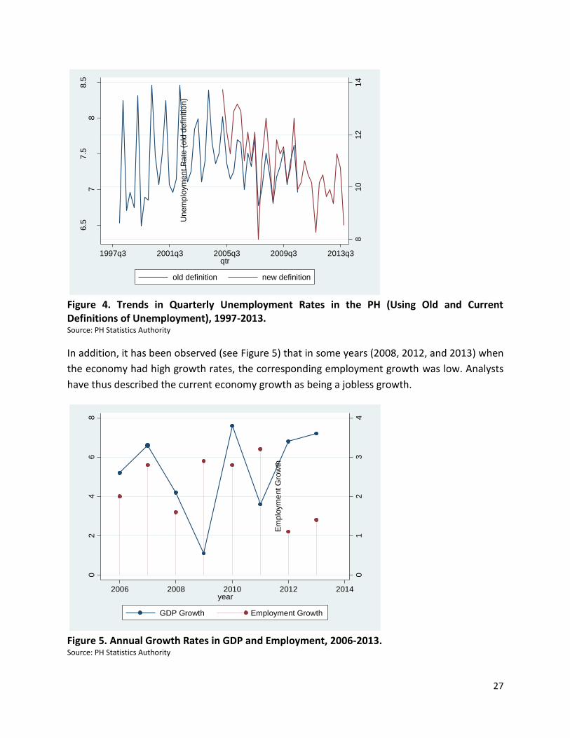
LFS. In 2004, the official definition of unemployment32 was changed by the Philippine Statistical

System to align it to suggestions made by the International Labor Organization. Unemployment

is currently defined as people who do not have work in the past week, have actively looked for

work, and are available for work. When we examine historical data on the unemployment rate

(total unemployed in relation to the labor force, which comprises the employed and

unemployed) we see that unemployment rates have been fairly stable across the years whether

using the current definition or the old definition of unemployment that did not include

availability for work (Figure 4).

32 Previous to 2004, the unemployed are persons 15 years old and over as of their last birthday and are reported as: (1) without

work, i.e., had no job or business during the basic survey reference period; AND (2) seeking work, i.e., had taken specific steps to look for a job or establish business during the basic survey reference period; OR not seeking work due to the following reasons: (a) tired/believe no work available, i.e., the discouraged workers who looked for work within the last six months prior to the interview date; (b) awaiting results of previous job application; (c) temporary illness/disability; (d) bad weather; and (e) waiting for rehire/job recall. After 2004, the definition of unemployment was changed. A third criterion must also be satisfied, aside from having no work, and actively seeking work --- being available for work, i.e., these persons should be available and willing to take up work in paid employment or self-employment during the basic survey reference period, and/or would be available and willing to take up work in paid employment or self-employment within two weeks after the interview date. This change in definition of the unemployed was carried in fulfillment of the National Statistical Coordination Board (NCSB) Resolution No. 15, Series of 2004, issued on 20 October 2004. International standards on this matter have been laid down in Resolution No. 1 adopted by the 13th International Conference of Labor Statisticians (ICLS) in October 1982 and expounded in the 1990 publication of the International Labor Organization (ILO), Surveys of Economically Active Population, Employment, Unemployment, and Underemployment: An ILO Manual on Concepts and Methods. It should be noted that out of 88 countries regularly conducting labor force surveys, in 2004, only 10 countries did not include the availability criterion, and the Philippines was the only country in Asia which did not use the availability criterion

27

Figure 4. Trends in Quarterly Unemployment Rates in the PH (Using Old and Current Definitions of Unemployment), 1997-2013. Source: PH Statistics Authority

In addition, it has been observed (see Figure 5) that in some years (2008, 2012, and 2013) when

the economy had high growth rates, the corresponding employment growth was low. Analysts

have thus described the current economy growth as being a jobless growth.

Figure 5. Annual Growth Rates in GDP and Employment, 2006-2013. Source: PH Statistics Authority

6.5

77.5

88.5

Un

em

plo

ym

en

t R

ate

(n

ew

defin

itio

n)

810

12

14

Un

em

plo

ym

en

t R

ate

(o

ld d

efin

itio

n)

1997q3 2001q3 2005q3 2009q3 2013q3qtr

old definition new definition

01

23

4

Em

plo

ym

ent G

row

th

02

46

8

GD

P G

row

th

2006 2008 2010 2012 2014year

GDP Growth Employment Growth

28

Noticeable also in Figure 5, during recent years when there was low GDP growth, particularly in

2009, ironically there was a surge in employment (and as will be shown later, the creation of

more jobs was actually a reaction of the labor market to economic slowdown, but the jobs

created here were largely of the vulnerable type of employment).

Aggregate pictures mask dynamics as was shown in the previous section. When indicators such

as official poverty rates have measly differences across time that are not statistically significant,

that does not necessarily mean that no poor person exits poverty as some

areas/subpopulations/sectors may be improving, and some may be deteriorating to yield a net

change of zero. In particular, some of the poor have become non-poor, but some non-poor fell

into poverty. Similarly, when unemployment rates are flat, does this mean no jobs are being

created given that the Filipino population, including our labor force33, continues to grow?

Disaggregating both employment and output data according to major sectors can be very

revealing (see Figure 6). The Philippines is dominated by the services sector, whether in output

or employment.

Figure 6. Output and Employment Shares in the Economy, by Major Sector; 1990-2013. Source: PH Statistics Authority

33 The Labor Force or Economically Active Population refers to the population 15 years old and over who contribute to the

production of goods and services in the country, and who are either employed or unemployed. Those who are not in the Labor Force refers to the population 15 years old and over who are neither employed nor unemployed, e.g. persons who are not working and are not available during the reference week and persons who are not available and are not looking for work because of reasons other than those previously mentioned. Examples are housewives, students, disabled or retired persons and seasonal workers.

0 20 40 60 80 100

201320122011201020092008200720062005200420032002200120001999199819971996199519941993199219911990

Output Share

Agriculture Industry Services

0 20 40 60 80 100

201320122011201020092008200720062005200420032002200120001999199819971996199519941993199219911990

Employment Share

Agriculture Industry Services

29

With regard to output, as of 2013, the share of services is more than half (57.7%) of total

national output. The output share of agriculture to the economy has always been relatively

minimal, 15.4% in 1990, and 11.2% in 2013. Even if we trace GDP shares of major sectors all the

way back to the 1946, we would find that the shares of agriculture, industry and services

sectors were then at 29.7%, 22.6%, and 47.7%, respectively, contrary to the belief of some that

we were once an agricultural economy. The economy has only become less agricultural in

recent times, with services and industry sectors getting more of the share of the economy.

As regards employment, the agriculture sector has also had decreasing trends in its share of

total employment from 45.2% in 1990 to about a third (31.0%) in 2013. In the same period, the

service sector took increasing shares of total employment from two-fifth (39.7%) to more than

half (53.4%). Industry, which had a share of about a 15.0% of aggregate employment in 1990,

had its share decrease slightly to 14.6% in 2009, and increase marginally to 15.6% by 2013.

In 2013, the largest growth in output of 9.5% came from industry, which had also the highest

growth in employment (3.4%), while agriculture, which only had a mere 1.1% growth in output,

even had a deceleration in employment figures. A structural transformation in the economy

may thus be arising, even if overall employment rate has been relatively flat.

Historically, the share of employment in industry has been lowest among the three major

sectors. Even the current robust growth in output of the industry sector has not translated into

more jobs (and lower unemployment) because of the low base figures of employment in the

industry sector. In the short term, for unemployment rates to drop considerably, employment

growth must occur in agriculture (which has a bigger share of employment than industry).

Volatility in employment (as well as in output) in agriculture, however, has been observed

especially on account of extreme weather events. In the long run, employment should start

shifting from agriculture to industry, the same path taken by many neighboring economies

which are in better development conditions.

Another disaggregation of employment in the country, by full-time and part-time

employment34, is equally revealing. Figure 7 shows that full-time employment in the Philippines

increased during periods of high economic growth (except for 2012) and contracted during

slowdown, while part-time employment has had reversed directions from those of economic

growth (except in 2008, the year when the slowdown in the global economy started to take

effect).

34 Those in full-time employment work 40 hours or more during the reference week, while those in part-time employment work less than 40 hours during the reference week.

30

Figure 7. Annual Growth Rates in GDP, Full Time and Part Time Employment, 2007-2013. Source: PH Statistics Authority

Thus, the economy isn’t really having jobless growth! In recent times, the small net changes in

the unemployment rates are the result of full-time jobs being created in the industry and

services sectors and part-time jobs lost in the agricultural sector. In addition, Figure 8 illustrates

a decreasing share of the total employment that is engaged in vulnerable work.

Figure 8. Proportion of Total Employment in Vulnerable Work (Unpaid Family Workers and Own-account Workers); 1998-2012. Source: PH Statistics Authority

-50

510

2006 2008 2010 2012 2014year

GDP Growth

Growth in Full-Time Employment

Growth in Part-Time Employment

01

02

03

04

05

0

Pro

po

rtio

n in V

uln

era

ble

Em

plo

ym

en

t (%

)

1995 2000 2005 2010 2015year

( as a percentage of total employment)

Unpaid Family Workers and Own-account Workers

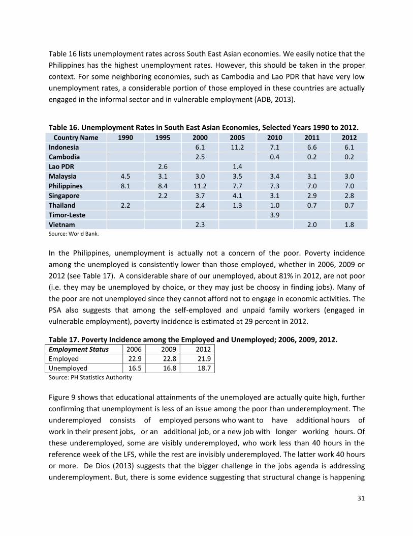
31

Table 16 lists unemployment rates across South East Asian economies. We easily notice that the

Philippines has the highest unemployment rates. However, this should be taken in the proper

context. For some neighboring economies, such as Cambodia and Lao PDR that have very low

unemployment rates, a considerable portion of those employed in these countries are actually

engaged in the informal sector and in vulnerable employment (ADB, 2013).

Table 16. Unemployment Rates in South East Asian Economies, Selected Years 1990 to 2012.

Country Name 1990 1995 2000 2005 2010 2011 2012

Indonesia 6.1 11.2 7.1 6.6 6.1

Cambodia 2.5 0.4 0.2 0.2

Lao PDR 2.6 1.4

Malaysia 4.5 3.1 3.0 3.5 3.4 3.1 3.0

Philippines 8.1 8.4 11.2 7.7 7.3 7.0 7.0

Singapore 2.2 3.7 4.1 3.1 2.9 2.8

Thailand 2.2 2.4 1.3 1.0 0.7 0.7

Timor-Leste 3.9

Vietnam 2.3 2.0 1.8 Source: World Bank.

In the Philippines, unemployment is actually not a concern of the poor. Poverty incidence

among the unemployed is consistently lower than those employed, whether in 2006, 2009 or

2012 (see Table 17). A considerable share of our unemployed, about 81% in 2012, are not poor

(i.e. they may be unemployed by choice, or they may just be choosy in finding jobs). Many of

the poor are not unemployed since they cannot afford not to engage in economic activities. The

PSA also suggests that among the self-employed and unpaid family workers (engaged in

vulnerable employment), poverty incidence is estimated at 29 percent in 2012.

Table 17. Poverty Incidence among the Employed and Unemployed; 2006, 2009, 2012. Employment Status 2006 2009 2012

Employed 22.9 22.8 21.9

Unemployed 16.5 16.8 18.7 Source: PH Statistics Authority

Figure 9 shows that educational attainments of the unemployed are actually quite high, further

confirming that unemployment is less of an issue among the poor than underemployment. The

underemployed consists of employed persons who want to have additional hours of

work in their present jobs, or an additional job, or a new job with longer working hours. Of

these underemployed, some are visibly underemployed, who work less than 40 hours in the

reference week of the LFS, while the rest are invisibly underemployed. The latter work 40 hours

or more. De Dios (2013) suggests that the bigger challenge in the jobs agenda is addressing

underemployment. But, there is some evidence suggesting that structural change is happening

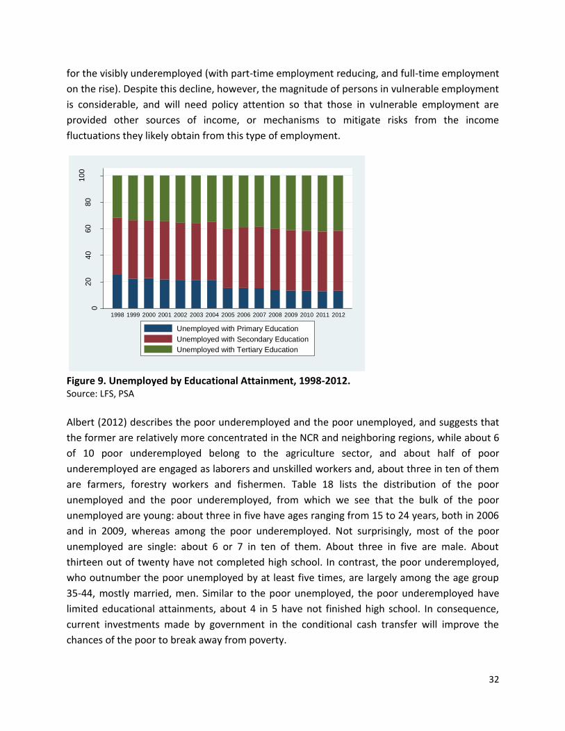
32

for the visibly underemployed (with part-time employment reducing, and full-time employment

on the rise). Despite this decline, however, the magnitude of persons in vulnerable employment

is considerable, and will need policy attention so that those in vulnerable employment are

provided other sources of income, or mechanisms to mitigate risks from the income

fluctuations they likely obtain from this type of employment.

Figure 9. Unemployed by Educational Attainment, 1998-2012. Source: LFS, PSA

Albert (2012) describes the poor underemployed and the poor unemployed, and suggests that

the former are relatively more concentrated in the NCR and neighboring regions, while about 6

of 10 poor underemployed belong to the agriculture sector, and about half of poor

underemployed are engaged as laborers and unskilled workers and, about three in ten of them

are farmers, forestry workers and fishermen. Table 18 lists the distribution of the poor

unemployed and the poor underemployed, from which we see that the bulk of the poor

unemployed are young: about three in five have ages ranging from 15 to 24 years, both in 2006

and in 2009, whereas among the poor underemployed. Not surprisingly, most of the poor

unemployed are single: about 6 or 7 in ten of them. About three in five are male. About

thirteen out of twenty have not completed high school. In contrast, the poor underemployed,

who outnumber the poor unemployed by at least five times, are largely among the age group

35-44, mostly married, men. Similar to the poor unemployed, the poor underemployed have

limited educational attainments, about 4 in 5 have not finished high school. In consequence,

current investments made by government in the conditional cash transfer will improve the

chances of the poor to break away from poverty.

020

40

60

80

10

0

pe

rcen

t

1998 1999 2000 2001 2002 2003 2004 2005 2006 2007 2008 2009 2010 2011 2012

Unemployed with Primary Education

Unemployed with Secondary Education

Unemployed with Tertiary Education

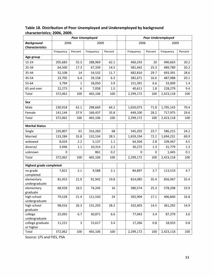
33

Table 18. Distribution of Poor Unemployed and Underemployed by background characteristics; 2006, 2009. Poor Unemployed Poor Underemployed

Background Characteristics

2006 2009 2006 2009

Frequency Percent Frequency Percent Frequency Percent Frequency Percent

Age group

15-24 205,683 55.3 288,969 62.1 460,243 20 490,663 20.2

25-34 64,500 17.3 67,339 14.5 581,442 25.3 489,789 20.2

35-44 52,108 14 54,532 11.7 682,816 29.7 693,391 28.6

45-54 23,705 6.4 29,158 6.3 382,671 16.6 487,988 20.1

55-64 3,794 1 18,050 3.9 151,391 6.6 33,009 1.4

65 and over 22,273 6 7,058 1.5 40,611 1.8 228,279 9.4

Total 372,062 100 465,106 100 2,299,172 100 2,423,118 100

Sex

Male 230,918 62.1 298,669 64.2 1,650,073 71.8 1,705,143 70.4

Female 141,144 37.9 166,437 35.8 649,100 28.2 717,975 29.6

Total 372,062 100 465,106 100 2,299,172 100 2,423,118 100

Marital Status

Single 226,807 61 316,260 68 545,202 23.7 586,215 24.2

Married 133,284 35.8 132,534 28.5 1,659,194 72.2 1,694,231 69.9

widowed 8,024 2.2 5,137 1.1 64,504 2.8 109,447 4.5

divorce/ 3,946 1.1 10,314 2.2 30,272 1.3 31,779 1.3

unknown 0 861 0.2 0 0 1,445 0.1

Total 372,062 100 465,106 100 2,299,172 100 2,423,118 100

Highest grade completed

no grade completed

7,822 2.1 9,588 2.1 84,897 3.7 113,519 4.7

elementary undergraduate

81,453 21.9 91,942 19.8 814,085 35.4 856,947 35.4

elementary graduate

68,928 18.5 74,245 16 580,574 25.3 578,208 23.9

high school undergraduate

79,528 21.4 111,550 24 392,904 17.1 406,840 16.8

high school graduate

98,016 26.3 131,293 28.2 332,403 14.5 361,292 14.9

college undergraduate

25,093 6.7 30,871 6.6 77,043 3.4 87,379 3.6

college graduate or higher

11,221 3 15,617 3.4 17,266 0.8 18,933 0.8

Total 372,062 100 465,106 100 2,299,172 100 2,423,118 100

Source: LFS and FIES, PSA

34

In consequence, as far as labor is concerned, the ultimate focus of government, and more

importantly the private sector (which is the main engine of the economy), should be on

creating quality jobs to sustain the growth momentum in the economy. But this focus cannot

be taken in isolation of required investments in education (both on the supply side and the

demand side).

5. Inequities in Basic Education

In the previous section, we noticed that underemployment and the quality of employment have

been barriers for improved income, especially for the poor. Inequalities in education

attainment have been the root of vulnerable employment, thus improving opportunities for

school participation and other education outcomes for the poor would be the mechanism for

social inclusiveness so that everyone, whether poor or non-poor, rural or urban folk, can fully

participate in economic growth processes and the progress of Philippine society.

Inequities in education are intrinsically important to address since these are unacceptable to

any society. Since the adoption of the Universal Declaration of Human Rights in 1948,

education, especially basic education, has been viewed as a human right. Various global human

rights treaties, such as the 1960 United Nations Educational, Scientific and Cultural Organization

(UNESCO) Convention against Discrimination in Education, the 1966 International Covenant on

Economic, Social and Cultural Rights (1966), the 1981 Convention on the Elimination of All

Forms of Discrimination against Women, and the 2006 Convention on the Rights of Persons

with Disabilities, have affirmed this view of education. In addition, the Education for All (EFA)

initiative and the Education Goals in the Millennium Development Goals (MDGs) also affirm the

right, particularly, of children to primary education. The High Level Panel (HLP) Report

(http://www.post2015hlp.org/accessible-report/) that initiated the emerging post 2015

Development Agenda on Sustainable Development Goals has also identified the importance of

education as a key driver for improving capabilities and opportunities for the poor, the

vulnerable and other marginalized sectors.

Education inequities limit people’s empowerment, capabilities and full participation in social

and, ultimately, in economic growth processes. The basic skills and competencies gained from

increased levels of education offer much better income prospects for rural folk, for those in the

informal sector, for those in vulnerable employment. More education also enables those in

paid formal employment to have higher wages. Psacharopoulos and Patrinos (2002) also

estimate that globally, every additional year of schooling yields generally 12% returns in wages,

although such returns vary considerably across countries and income levels. Higher incomes

brought about by improved education attainment ultimately boost innovation and higher

productivity, which, in turn, drive growth in an economy (Barro, 2013).

35

The latest report of ADB (2014) on a framework for inclusive growth discusses the importance

of education as a pathway for inclusive growth. In the report, estimates of education poverty

rates and extreme education poverty rates are presented for select countries, including the

Philippines. Table 19 shows that between 1993 and 2008, the proportion of the youth (aged

15–24) in the country with less than 4 years of schooling (called education poverty rate) had

hardly changed from 5.3% in 1993 to 4.9% in 2008. Wealth, gender and rural-urban disparities

are challenges to achieving equity in years of schooling of the youth. Notice that the males are

more education poor than females, rural areas are more education poor, and the share of our

youth with less than 4 years of schooling among the poor (19.0%) was as much as four times

the national average (5.3%). Extreme education poverty, or the proportion of the youth with

less than 2 years of schooling, was also unchanged at 1.9% from 1993 to 2008, and similarly

have gender, wealth and rural-urban disparities that need to be addressed. The country also

has had little improvements in years of schooling among the youth in the period 1993 to 2008,

before government expanded the coverage of Pantawid.

Table 19. Proportion of Youth Aged 15 -24 in the Philippines with less than 4 years of schooling (education poverty rate) and less than 2 years of schooling (extreme education poverty rate), 1993 and 2008.

Extreme Education Poverty Rate Education Poverty Rate

1993 2008 1993 2008

Lowest Quintile 7.2 19.0 7.2 18.8

Highest Quintile 0.6 1.2 0.3 0.7

Rural 3.0 8.5 3.2 7.9

Urban 1.0 2.7 0.7 2.3

Male 2.1 6.7 2.2 6.5

Female 1.7 3.9 1.6 3.3

National 1.9 5.3 1.9 4.9 Note: Taken from ADB (2014). Estimates prepared by ADB staff using data from 1993 and 2008 National

Demographic Health Survey, conducted by PSA.

A report on Out of School Children (OOSC) 35 prepared by PIDS (2012) for UNICEF and DepED

suggests that in school years 2007-2008 and 2008-2009, estimates of school participation in the

Philippines vary depending on the data source (see Table 20). In school years 2007-2008 and

2008-2009, administrative data from the Department of Education (DepED) together with

projections of school-age children suggest that school participation of primary age children at

the primary level was around 90% (while survey-based estimates are around 95%). School

participation rates of secondary age children at the secondary level are estimated at around

60% also from the administrative data (while survey based estimates are around 5 percentage 35 Out of school children refer here to (a) five year old children who are not in preprimary or primary school; (b) children of primary-school age (6 to 11) who are not in primary school or secondary school; and (c) children of secondary-school age (12-15) who are not in primary school or secondary education.

36

points higher, i.e. 65%). The statistics on school participation from surveys in Table 20 yield an

estimated number of five to fifteen-year-old OOSC at 2.9 million in 2008-2009.

Table 20. School Participation/Attendance Rates in 2007 and 2008 by Age and by Data Source

Age Group 2007 2008

BEIS APIS LFS July UIS BEIS APIS LFS July FLEMMS LFS Oct UIS 5 Years Old 47.9a 67.2 67.3 56.3a 65.8 65.9 - 65.9 Primary Age (6 to 11 years old)

88.3b

(88.7c) 94.4

(89.8d) 93.8 87

(88c) 89.2b

(89.6c) 95.2

(90.8d) 94.9 92.3

(85.2d) 94.8 88

(88c) Secondary Age (12 to 15 years old)

59.9b (59.9c)

88.5 (65.8 d) 87.8 60

60.5b (60.5c)

89.6 (66.3d) 90.0

87.2 (60.1d) 88.9 61

Notes: a based on BEIS enrollment in public and private kindergarten schools, as well as DSWD data on children served in day care centers; b based

on revised projections of school-age population; c adjusted net enrollment ratio (ANER) is the ratio of the number of children in an age range that is

enrolled in the proper education tier (or higher) relative to the number of children of the school-age range; d adjusted net attendance rates (ANAR) is

the ratio of the number of children in an age range that attends the proper education tier (or higher) relative to the number of children of the school-age

range

Recent waves of the APIS suggest that the number of five to fifteen-year-old OOSC have

decreased to 2.6 million by 2010, and further to 1.8 million by 2011. The decrease in OOSC is

largely on account of the increase in school participation of 5 to 14 year old children, on

account of the Pantawid Pamilya Pilipino Program (4Ps), the conditional cash transfer (CCT)

program implemented by government. Pantawid was designed to assist poor households to

break free from intergenerational poverty by investing in the education of their children, and

health of their household members.

Household surveys ask the reasons why children are not in school. Table 21 lists these reasons

among five year old OOSC and among primary school-age children in 2007 and 2008.

Table 21. Percentage of Five year old and Primary School-Age OOSC in 2007 and in 2008, by Reason for Nonattendance in School, by Data Source.

Reason for Nonattendance Five year old Children (%) Six to eleven year old Children (%)

APIS 2007 APIS 2008 APIS 2007 APIS 2008 FLEMMS 2008

Lack of personal interest 3.83 6.94 24.49 31.68 23.78

High cost of education 4.53 3.62 12.90 11.52 13.32

Too young to go to school 83.52 80.46 34.03 29.21 34.86

Illness/disability 0.54 1.06 8.08 9.48 6.76

Lack of nearby schools 4.53 3.88 8.61 7.45 7.66

Employment 0.00 0.00 0.31 0.13 0.09

Other reasons (e.g., school records, marriage*, housekeeping)

3.05 4.04 11.55 10.53 13.53

Source: APIS 2007, APIS 2008, and FLEMMS 2008, PSA; *including marriage by children

In both 2007 and 2008, about four out of every five were viewed as too young for schooling. In

2007, among five year old OOSC, about one out of twenty-five was reported to lack interest,

while in 2008, this rate increased to one out of fifteen. When data are further disaggregated

into urban and rural areas, we find that in 2007 and 2008, another prominent reason cited in

urban areas, aside from being too young or lacking interest was cost of schooling. In the rural

areas, on the other hand, school accessibility was the more prominent reason for

nonattendance of five year old children. The reasons for nonattendance of five year old

37

children hardly varied by sex: the share of boys (82.9 percent) that were too young for

schooling is practically the same as that of girls (77.5 percent).

Among primary school-age children (aged six to eleven), about three-fifths of primary school-

age children were not in school either because the children were thought to be too young for

schooling (especially among six year old and seven year old children) or because the children

lacked personal interest. About ten percent of six to eleven year old children were not in

school because of cost issues while five percent were not in school due to school accessibility

issues (with the figures higher in rural areas). Among boys six to eleven years old who were not

in school, the primary reason for being out of school was lack of interest while among girls of

the same age group, the major reason for nonparticipation continued to be that the child was

considered too young for schooling.

A logistic regression model36 explaining lack of interest in school (see Table 22) suggests that

the mother’s level of education explains some of this lack of interest along with advancing age

and having a male household head. Some qualitative investigations suggest that while parents,

principals, and teachers report that some parents do not support their children’s schooling,

majority of the parents do. Mothers tend to spend time with children who are in the younger

grades, helping them with the children’s assignments, projects, and accompanying them to

school every day. The mother guides the children through school assignments until at least the

middle of primary school. Field work and Table 22 show that a child’s lack of interest for

schooling is a capacity issue on the part of the parent (especially the mother), which ultimately

affects the child’s interest in schooling. Thus, special school-based interventions like remedial

classes for children who are behind in reading or math skills, can augment shortcomings in

support provided by mothers. In the higher grades, however, parents who have little education

need to provide at least emotional and resource support. It can be unreasonable to expect

parents with little or no education to be able to provide similar quality support provided by

more educated parents. These parents may not even attend parent-teacher association (PTA)

meetings or may not show up when guidance counselors call them in as they find it difficult to

understand what is going on and more importantly, they really cannot afford to take time out 36 A logistic regression explains a binary outcome (here, whether a child not in school lacks interest or is not reported to lack interest) from a set of explanatory variables 𝑋1, 𝑋2, … , 𝑋𝑘, that may be binary, continuous, or a mix of any of these. The relationship between the binary response variable and the explanatory variables is given by:

𝑙𝑜𝑔 (𝜃

1 − 𝜃) = 𝛽0 + 𝛽1 𝑋1 + 𝛽2𝑋2 + ⋯ + 𝛽𝑘𝑋𝑘

where θ and 1−θ respectively represent the probability of being an OOSC and the probability of attending school. Note also that for categorical explanatory variables, a set of binary indicator variables are first generated to represent membership (or non-membership) in the categories, with one of the indicator variables serving as base or reference to compare other categories with.

38

from work, unlike parents with more education who may have better capacity to take time off

from their occupations to attend to these matters.

Table 22. Log Odds of Logistic Regression Model Predicting Lack of Interest. Explanatory Variables Lack of

interest Log per capita expenditure of household -0.02

Indicator for Age = 7 (base Age = 6) 1.45***

Indicator for Age = 8 1.59***

Indicator for Age = 9 1.56***

Indicator for Age = 10 1.69***

Indicator for Age = 11 1.60***

Mean pupil-teacher ratio in region 0.00

Urban indicator (rural base) -0.26

Female child Indicator (male base) -0.37**

Number of children in household 0.01

Number of adults in household 0.09

Number of retired persons in household 0.00

Mother has some secondary education (base mother at most primary)

-0.57**

Mother has beyond secondary education (base mother at most primary)

-0.91**

Indicator for male household head -0.29

Age of household head 0.00

Constant -1.16 Source: Calculations using data from BEIS 2008—09 (census of public schools) and APIS 2008 (APIS n=40,613) Note: *p<.05; **p<.01; ***p<.005

Another logistic regression to identify determinants of the lack of school participation is

provided in Table 23. The basic source for the model is data from the 2008 APIS, supplemented

by average pupil-to-teacher ratios (PTRs) in the regions sourced from the 2008-09 BEIS. The

PTR, which for the primary school level, is the ratio of the total number of students enrolled in

primary school to the total number of primary school teachers, is a proxy for quality of

schooling. (Lee and Barro, 1997). The higher the PTR, the lower the relative access of students

to teachers and the less attention provided by the teacher to students, especially for students

who may need more attention than others and are therefore more likely to lose interest in

schooling. A parental perception of overcrowding may also influence the decision to allow their

children to attend school. Various individual and household characteristics can also explain lack

of school participation. The explanatory variables considered in the logistic regression model,

include: (1) individual characteristics, namely, the sex and age of the child; (2) household

characteristics, including household per capita expenditure (in logarithmic terms) and the

number of children, adults, and retired persons in the household; location of household

residence (urban/rural); age of the household head; sex of the household head; educational

39

attainment of the child’s mother; and, (3) average PTR in the region. A separate regression was

run for primary school-age and for secondary school-age children, with the latter model

including in its list of explanatory variables an indicator on whether or not the child is engaged

in labor.

Table 23. Log Odds of Logistic Regression Models for Nonattendance in School.

Explanatory Variables Primary- School

Age Secondary-School Age

Log ( per capita expenditure) -0.498*** -0.873***

Indicator for Age = 6 (BASE)

Indicator for Age = 7 -2.228***

Indicator for Age =8 -3.086***

Indicator for Age = 9 -3.476***

Indicator for Age = 10 -3.412***

Indicator for Age = 11 -3.223***

Indicator for Age = 12 (BASE)

Indicator for Age = 13 0.552***

Indicator for Age = 14 1.073***

Indicator for Age = 15 1.300***

Mean Pupil to Teacher Ratio in Region (Elementary Level)

0.035***

Mean Pupil to Teacher Ratio in Region (High School Level)

0.005**

Indicator for Residing in Urban Area 0.064 -0.182**

Indicator for Female -0.295*** -0.567***

Indicator for Mother Attaining At Most Primary (BASE)

Indicator for Mother Attaining Secondary Education -0.680*** -0.796***

Indicator for Mother Attaining Education Beyond Secondary Level

-0.538*** -1.451***

Indicator for Male household Head -0.223* -0.275**

Age of Household Head 0.006 0.007

Number of Children in Household 0.065*** 0.006

Number of Adults in Household 0.016 -0.029

Number of Retired Persons in the Household -0.085 -0.223

Child Engaged in Labor 1.956***

Memo Notes:

Number of Observations 20809 14373

Pseudo Rsquared 0.2844 0.2517 Source: Calculations based on data from BEIS 2008-2009 and APIS 2008

The logistic regression model shows that, assuming all other explanatory variables are constant

(ceteris paribus):

Children who come from families with more per capita expenditure are more likely to be in school. For primary school-age children, every one percentage change in per

40

capita expenditure is associated with a 0.50 percent decrease in the odds for not attending school. For secondary school-age children, the decrease in odds for not attending school is 0.87 percent;

Age matters. Compared to six-year-old children, children aged seven to eleven years old are less likely to be out of school. Secondary school-age children in the thirteen-to-fifteen-year-old age range are more likely to be OOSC than twelve-year-old children;

Every unit increase in pupil-to-teacher ratio is associated with an increase in the odds of nonattendance in school by 3.5 percent in primary school-age children and 0.5 percent in secondary school-age children;

Secondary school-age children residing in rural areas are more at risk of being out of school compared to children residing in urban areas. Urban-rural differentials are not significant for primary school-age children;

Boys are more at risk of being out of school. Primary school-age girls are 1.3 times more likely to be in school than their boy counterparts; secondary school-age girls are 1.8 times more likely to attend school than boys in their age range;

Compared to children with mothers who have attained, at most, primary level of education, children with more educated mothers tend to be less prone to being out of school;

Children belonging to families with many children are more at risk of being out of school;

Secondary school-age children who are not engaged in some labor activities are more likely to be in school. Those engaged in child labor are seven times more likely to be out of school; and

Primary school- and secondary school-age children who are part of families where the household head is male tend to be less at risk of being OOSC.

6. Investing in Human Capital: the CCT

Whether we examine the lack of school participation, or the lack of interest in schooling, these

phenomena are largely economic, and would thus require some economic intervention.

Pantawid, the government’s CCT has been designed precisely to address this, to provide

incentives to poor households to compensate for the income they lose by sending their children

to school instead of having them work at an early age. In addition, CCT household beneficiaries

are given cash grants to incentivize them to send their household members (especially pregnant

women and children) to avail of health services. The CCT is a concrete step to ensure children’s

rights to a full life that were articulated in Convention on the Rights of the Child and adopted by

United Nations General Assembly on Nov. 20, 1989.

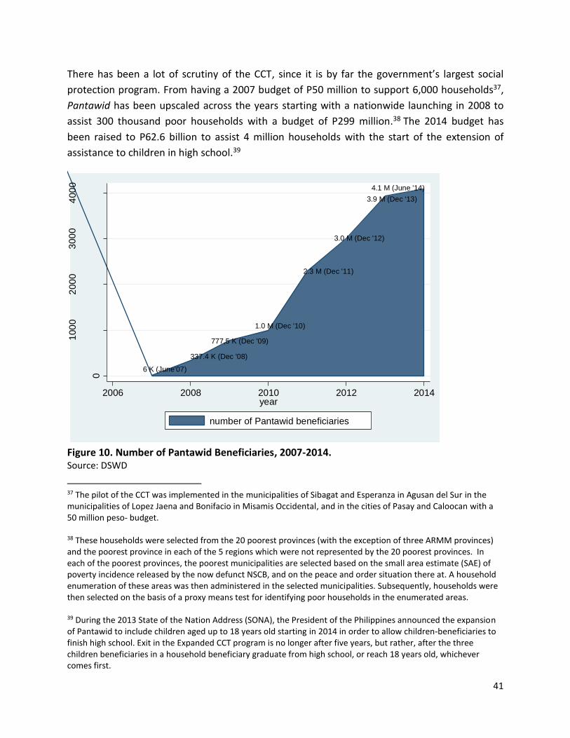
41

There has been a lot of scrutiny of the CCT, since it is by far the government’s largest social

protection program. From having a 2007 budget of P50 million to support 6,000 households37,

Pantawid has been upscaled across the years starting with a nationwide launching in 2008 to

assist 300 thousand poor households with a budget of P299 million.38 The 2014 budget has

been raised to P62.6 billion to assist 4 million households with the start of the extension of

assistance to children in high school.39

Figure 10. Number of Pantawid Beneficiaries, 2007-2014. Source: DSWD

37 The pilot of the CCT was implemented in the municipalities of Sibagat and Esperanza in Agusan del Sur in the municipalities of Lopez Jaena and Bonifacio in Misamis Occidental, and in the cities of Pasay and Caloocan with a 50 million peso- budget. 38 These households were selected from the 20 poorest provinces (with the exception of three ARMM provinces) and the poorest province in each of the 5 regions which were not represented by the 20 poorest provinces. In each of the poorest provinces, the poorest municipalities are selected based on the small area estimate (SAE) of poverty incidence released by the now defunct NSCB, and on the peace and order situation there at. A household enumeration of these areas was then administered in the selected municipalities. Subsequently, households were then selected on the basis of a proxy means test for identifying poor households in the enumerated areas. 39 During the 2013 State of the Nation Address (SONA), the President of the Philippines announced the expansion of Pantawid to include children aged up to 18 years old starting in 2014 in order to allow children-beneficiaries to finish high school. Exit in the Expanded CCT program is no longer after five years, but rather, after the three children beneficiaries in a household beneficiary graduate from high school, or reach 18 years old, whichever comes first.

6 K (June'07)

337.4 K (Dec '08)

777,5 K (Dec '09)

1.0 M (Dec '10)

2.3 M (Dec '11)

3.0 M (Dec '12)

3.9 M (Dec '13)

4.1 M (June '14)

0

100

02

00

03

00

04

00

0

num

ber

of b

en

eficia

rie

s (

in th

ou

sa

nd

s)

2006 2008 2010 2012 2014year

number of Pantawid beneficiaries

42

Many have criticized the CCT from various angles: its cost, its targeting system, and the entire

scheme of giving support to the poor. While the program is costly in aggregate, but the

amounts given to each Pantawid household beneficiary has not been much. Using data from

the APIS 2013, the World Bank estimated that in 2013, Pantawid beneficiary families received

an average of P1,407 of monthly cash grants, if they sent their 3 beneficiary children to school,

and received health services for their household members. Without the cash grants, these

families had an average per capita income of P13,293, whereas the poverty line per person

then was P19,262. Thus, the amounts given will not really help them cross the poverty line, but

are only truly “Pantawid.”

Some argue that the money given to the poor only go to alcohol, but hard data, from

independent evaluations, show otherwise. About half of cash grants are used for food, a

quarter (25%) on education-related expenses, while 7% is used on health, and close to nothing

is used for recreation or alcohol.

Some also suggest that Pantawid has not brought down poverty rates, and is thus ineffective.

Actually, Pantawid was not designed to be a quick fix to reduce poverty. In 2012, poor families,

which have an average family size of 6, needed, on average, P29,765 to cross the poverty line,

while CCT beneficiary families only received a maximum of PHP 15,000 grants in 2012 (PHP 300

per child per month for 10 months for a maximum of 3 children, plus PHP 500 per month for

twelve months for health support), if they satisfied their co-responsibilities. Pantawid was

meant as a human capital investment, i.e., to encourage the poor to send their children to

school so that they can, in the future, find a means of escaping the cycle of poverty. These

beneficiary children are still in school, and it is expected that with more schooling, they will

have better income prospects once they join the labor market.

Using data from the 2013 APIS, the World Bank has suggested that the official poverty rate (of

25% in the first semester of 2013) could be as much 26.4% without Pantawid. Even the extreme

poverty rate (of 11.1%), would be 1.4 percentage points higher without Pantawid (12.5%).

Table 25. Estimates of Poverty Incidence (using Total Poverty Line and Food Poverty Line)

with and without Pantawid Pamilya.

National Among Pantawid beneficiaries

Without Pantawid

With Pantawid

Without Pantawid

With Pantawid

Poverty rate 26.4% 25.0% 64.5% 58.1%

Extreme poverty rate

12.5% 11.1% 35.3% 28.7%

Note: Estimates generated by World Bank Staff using data from national household surveys conducted by PSA, as

presented in DSWD forum on Pantawid Pamilya 2nd Wave Impact Evaluation, Nov 14, 2014.

43

Among CCT beneficiaries, the increase in poverty rate without Pantawid is even higher. Poverty

among beneficiaries (at 58.1%) would be 6.4 percentage points higher (64.5%) without the CCT.

Doesn’t this suggest that some CCT households are not “poor”? Certainly, but independent

evaluation by the Social Weather Stations shows that most of these non-poor beneficiaries are

nearly-poor. Note that while government estimates poverty through income data collected

meticulously in surveys of the PSA, the DSWD, through their Listahanan, on the other hand,

obtains information on facilities (such as electricity, toilets, walls, roofs) and assets (such as

refrigerators, television sets, and the like), and on the basis of a statistical model estimates

household income. There are certainly errors in identifying poor households (when a non-poor

household is thought to be poor, or a poor household is tagged as non-poor), but DSWD has a

process for delisting the non-poor, and also for having the poor who are not in its list to be

enlisted, subject to verification. Further, the World Bank estimates that more than four fifths

(82%) of Pantawid beneficiaries are from the bottom 40 percent of income distribution, and

more than half (53%) are from the bottom 20 percent. Figure 11 shows that when Pantawid is

compared in targeting accuracy with other CCTs, the DSWD program performs better than all

CCTs with a large coverage in the population (of more than 15%), except for that of Brazil.

Figure 11. Targeting accuracy to the poorest 20 percent of CCTs with more than fifteen

percent coverage of the population.

Note: Estimates generated by World Bank Staff, as presented in DSWD forum on Pantawid Pamilya 2nd Wave

Impact Evaluation, Nov 14, 2014.

57.0

52.850.4

40.639.5

37.0

02

04

06

0

% b

en

eficia

ries f

rom

th

e p

oore

st 2

0%

Brazil (2009)

Philippines (2

013)

Mexico (2010)

Jamaica (2010)

Colombia (2012)

Ecuador (2010)

44

The World Bank also estimates using APIS 2013 data that Pantawid has increased income of

beneficiaries so that they have moved closer to the poverty line: per peso cash grant, the

poverty gap has been reduced by 61 centavos. It is no wonder why many serious poverty

analysts are convinced that had we implemented Pantawid a decade ago, we would be reaping

benefits of lower poverty incidence, lower poverty gap and lower income inequality today.

There are certainly challenges in making economic growth inclusive and in making prosperity

shared. The CCT is a worthy program to protect the poor from getting forever trapped in

poverty by investing in their human capital, but in isolation, it will not be enough, especially in

the short term, to reduce poverty. We all have roles to play, especially our taipans, in improving

the economic mobility of those at the lower end of income distribution. The year 2015, the

target year for the MDGS, is fast approaching, and as the world starts crafting and embarking

on a post-2015 agenda, we have to ensure that no one, whether poor or nonpoor, male or

female, urban or rural folk, Christian or Muslim, employed or unemployed, is left behind in

development.

References

Albert, J. R. G. (2008). “Issues on Counting the Poor” PIDS Policy Notes 2008-11 (Available from Internet

http://dirp4.pids.gov.ph/ris/pn/pidspn0811.pdf Last accessed 31 July 2014 ) .

Albert, J. R. G. (2012). “May trabaho na nga, mahirap pa ren… JEP Jobs, Earnings, Prices para sa Kanila”

in Sexy Statistics Series, NSCB Blog, 22 October, 2012 (Available from Internet

http://www.nscb.gov.ph/sexystats/2012/SS20121022_joblessness.asp Last accessed 31 July 2014 ) .

ADB (2012). Framework of Inclusive Growth Indicators 2012: Key Indicators for Asia and the Pacific,

Special Supplement, 3rd Edition, Asian Development Bank, Manila, Philippines.

ADB (2014). Framework of Inclusive Growth Indicators 2012: Key Indicators for Asia and the Pacific,

Special Supplement, 3rd Edition, Asian Development Bank, Manila, Philippines.

Balisacan, A. and Fuwa, N. (2004).

Going Beyond Cross-Country Averages: Growth, Inequality and Poverty Reduction in the Philippines

Cord, L. Lopez, J. H. and Page, J. (2003). “When I Use a Word… Pro-Poor Growth and Poverty

Reduction”. (Available from Internet

http://siteresources.worldbank.org/INTPGI/Resources/15179_Page_Lopez_Cord_-

_When_I_use_a_word.pdf Last accessed 31 July 2014 )

45

Datt, G. and M. Ravallion (1992). "Growth and Redistribution Components of Changes in Poverty

Measures: A Decomposition with Applications to Brazil and India in the 1980s." Journal of Development

Economics, 38, 275-295.

De Dios, E. (2013). “Unemployment has no welfare significance” in Introspective, Business World, 30

September, 2013 (Available from Internet

http://www.econ.upd.edu.ph/perse/?p=3178 Last accessed 31 July 2014 ) .

Martinez, A., Western, M., Haynes, M. and Tomaszewski, W. 2014a. Is there income mobility in the Philippines? Asian-Pacific Economic Literature, 28(1), pp. 96-115. DOI: 10.1111/apel.12047. Martinez, A., Western, M., Tomaszewski, W. and Haynes, M. 2014b. How Income Segmentation Affects Income Mobility: Evidence from Panel Data in the Philippines. Working paper under review in a journal.

Ostry, J. D. & Berg, A. (2011.) "Inequality and Unsustainable Growth; Two Sides of the Same Coin?," IMF

Staff Discussion Notes 11/08, International Monetary Fund. (Available from Internet

http://www.imf.org/external/pubs/ft/sdn/2011/sdn1108.pdf Last accessed 31 July 2014)

Picketty, T. (2014). Capital in the Twenty-First Century. Harvard University Press.

Ravallion, M. (2013), How Long Will It Take to Lift One Billion People Out of Poverty? (Available from

Internet

http://www-

wds.worldbank.org/external/default/WDSContentServer/IW3P/IB/2013/01/22/000158349_2013012209

1052/Rendered/PDF/wps6325.pdf Last accessed 30 November 2014 )

Reyes, C. and Tabuga, A. (2011), A note on economic growth, inequality, and poverty in the Philippines.

PID Discussion Paper 2011-30. (Available from Internet

http://dirp3.pids.gov.ph/ris/dps/pidsdps1130.pdf Last accessed 31 July 2014)

Thomas, V., Albert, J. R. G., and Hepburn, C. (2014). Contributors to the frequency of intense climate

disasters in Asia-Pacific countries. Climatic Change (2014) 126:381–398. DOI 10.1007/s10584-014-1232-

y (Available from Internet

http://download.springer.com/static/pdf/187/art%253A10.1007%252Fs10584-014-1232-

y.pdf?auth66=1418267014_6a89ec2b4619fda2c9cff46676237425&ext=.pdf Last accessed 30 November

2014 )

Thomas, V., Albert, J. R. G., and Perez, R. (2013). Climate-Related Disasters in Asia and the Pacific. ADB

Economics Working Paper Series No. 358. July 2013. (Available from Internet

http://www.adb.org/sites/default/files/publication/30323/ewp-358.pdf Last accessed 31 July 2014 )

World Bank (2014). Philippine Economic Update, August 2014 edition

46

http://www.worldbank.org/en/country/philippines/publication/philippines-accelerating-public-

investment-to-sustain-growth-that-benefits-the-poor Last accessed 30 November 2014

World Bank (2013). Philippine Economic Update: Accelerating Reforms to Meet The Jobs Challenge

(Available from Internet

http://www.worldbank.org/content/dam/Worldbank/document/EAP/Philippines/Philippine_Economic_

Update_May2013.pdf Last accessed 31 July 2014 )

World Development Indicators. 2014. World Development Indicators Database. The World Bank. Available at http://data.worldbank.org/data-catalog/world-development-indicators