Inequality decomposition by factor component: a newapproach illustrated on the Taiwanese case

Martin FOURNIER*

CERDI (Université d’Auvergne) and CREST (Laboratoire deMicroéconométrie)

Key Words: Inequality, Income distribution, Inequality decomposition byfactor components, Taiwan.

Classification JEL: D3, D63, O15, O53

Address: CERDI65, bd François Mitterrand63000 Clermont-Ferrand

E-mail: M.Fournier@cerdi.u-clermont1.frTél.: 04 73 43 12 29

This version: November 1999

* I would like to thank François Bourguignon, Denis Fougères, François Gardes, Sylviane

Guillaumont-Jeanneney, Marc Gurgand and Sylvie Démurger as well as participants at seminars inCERDI and CREST for helpful comments.

2

1. Introduction

The rise in inequality observed in most industrialised countries andspecifically in the United States has lead to rising concern for distributionalissues since the beginning of the 90s (Atkinson, 1997; Atkinson andBourguignon, 1998; Kanbur, 1999; Kanbur and Lustig, 1999). Parallel tothe development of theoretical and empirical works, methodological issueshave recently been raised, leading to the elaboration of new tools for theanalysis of the sources of changes in the distribution of income. Inequalitydecomposition methods have been developed in two main directions, oneinitiated by Juhn, Murphy and Pierce’s (1993) work on decompositionmethods based on micro-simulation techniques, the other in the line ofDiNardo, Fortin and Lemieux’s (1996) paper, based on non-parametricweighting techniques. However, both methods are focussed on inequalitydecomposition by population sub-groups and bring little perspective aboutthe decomposition of inequality by factor component1.

The question of the relative importance of various income sources inthe level, and in the distribution, of total income is nonetheless a centralaspect of the analysis of observed changes in income inequality. Indeed,inequality decomposition by factor component allow for an evaluation ofthe specific impact of a given income source (capital income for example)on total income inequality. Moreover, it gives valuable information on theevaluation of the impact on the distribution of total household income ofchanges in household structure as well as changes in labour forceparticipation behaviours2. This feature has been at the core of variousempirical studies of the rise in income inequality in the US, which point outchanges in household structure and participation behaviours as centralfactors3. Usual factor decomposition of income inequality is howeverrestricted to some specific inequality index and suffers from a number oflimitations highlighted by Shorrocks (1982) theorem.

In a recent work, Burtless (1999) studies the impact of changes in thecorrelation between spouses' income on US household inequality using analternative methodology. We show in this paper that the method succinctlyand intuitively exposed by Burtless on a specific empirical framework canbe systematised into a general decomposition methodology allowing toovercome a number of drawbacks inherent to the use of usualdecomposition procedures. This method, which we will call rank-correlation method, does not rely on any parametrical assumptions andprovides easily interpretable results as is shown by the illustration driven onthe Taiwanese case provided by the second part of this paper.

After a decrease in inequality since the beginning of the 50s, Taiwanhas experienced a worsening of household income distribution since the endof the 70s. Bourguignon, Fournier and Gurgand (1999a) show that animportant part of the observed rise in inequality can be imputed to changes

3

occurring within the structure of households. Several other studies alsoinsist on the unequalizing effect due to rising endogamy in terms ofeducation in the assortative mating of spouses in Taiwan (Fields and Leary,1997; Tsai, 1994). However, usual procedures fail to provide a specificevaluation for the magnitude of this phenomenon. The second part of thispaper proposes a new study of this issue through the implementation of therank-correlation method on Taiwanese data over the 1979-94 period.

The paper is organised as follows. Section 2 discusses theoreticalresults concerning usual methods for inequality decomposition by factorcomponents and proposes a generalisation of the alternative approachinitiated by Burtless (1999). Section 3 applies this method to incomedistribution changes in Taiwan over the 1979-94 period. Section 4concludes and discusses further methodological developments to be derivedfrom this approach.

2. À new approach to inequality decomposition by factor component

2.1 Usual decomposition procedures: Shorrocks' theorem

Usual inequality decomposition by factor components can beformalised as follows. Let Y be total income derived from N distinct incomesources:

(1) Y Ykk

N

==

∑1

and let I be an inequality index. Decomposing inequality by factorcomponents consists in deriving a set of N contributions ( ) ...Sk k N=1 suchthat:

a) Sk is a function of the distribution of the kth income source -written {Yk} - and of its relative share in total income (πk).

b) { } ),()( kk

N

1kk YSYI π∑

=

=

Sk thus represents the kth income source contribution to observed inequalityin total income Y.

Two main approaches can be found in the literature. The firstincludes works based on the decomposition of the variance of income and,following Fei, Ranis and Kuo (1978), on the decomposition of the Ginicoefficient. This approach tries to define easy to apply and intuitivelyappealing decompositions but remains based on ad hoc formulations. Thesecond approach follows Shorrocks (1982) formalisation of inequality

4

decomposition by factor components through the definition of a set ofaxioms leading to a general decomposition procedure.

Variance decomposition

The usual decomposition4 of the variance allows for relatively simplefactor decomposition for the variance as well as most inequality measuresderived from the variance (especially the coefficient of variation). Indeed,the variance of total income Y can be written as the following function of thestandard errors of sources (σk) and of the covariance between sources (Cov):

(2)

∑

∑∑∑

=

≠ ==

=

+=

N

1kk

jk

N

1jkj

N

1k

2k

YYCov

YYCovY

),(

),()²( σσ

which directly provides the Sk contributions for the variance of total income,),( kk YYCovS = .

This decomposition directly applies to the square of the coefficientof variation as follows:

(3)

∑=

=

=

N

1k

k

2

YYCov

YYCV

²),(

²)²()(

µ

µσ

which provides an evaluation of the contribution of various income sourcesto overall observed inequality. Moreover, it should be noted here that therelative contribution of income sources is the same for the variance or thecoefficient of variation, since in both cases we have:

(4))²(

),()()(

YYYCov

YIYSs kkk

k σ==

Gini coefficient decomposition

Following Fei, Ranis and Kuo (1978), Pyatt, Chen and Fei (1980)proposed a decomposition procedure for the Gini coefficient as a weightedsum of « pseudo-Gini » terms ( ~Gk ), using the relative share of sources intotal income as weights (Φk), so that:

5

(5)∑∑

∑ ===

i

ii

ik

k

N

kkk Y

YwhereGYG φφ ,~)(

1

« Pseudo Gini » coefficient ~Gk is computed as a Gini coefficient over thekth income source (Yk), individuals (or any other unit) being ranked in termsof total income (Y) and not in terms of the kth income source.

Pyatt, Chen and Fei (1980) also show that « pseudo Gini »coefficients can be written as a function of individuals ranks in terms oftotal income (ρ) and of the kth income source (ρk) as follows:

(6)),(),()(),(~

kk

kkkk YCov

YCovYGYYGρρ=

The Gini coefficient can thus be written as a weighted sum of Ginicoefficients computed (in the usual way) on various income sources asfollows:

(7) ∑=

=N

1kk

kk

kk YG

YCovYCovYG )(

),(),()(

ρρφ

Equation (7) allows for a decomposition of the Gini coefficient intothe sum of terms depending solely on the distribution of a specific incomesource and its correlation with total income. Here, as for the decompositionof the variance of total income, each contribution can be positive as well asnegative. A negative sign refers to a negative correlation between theincome source and the rank with respect to total income, which means thatthe income source lowers total income inequality (this will be the case forexample for transfers).

Shorrocks’ theorem: an impossibility theorem

Shorrocks (1982) proposes a formalisation for inequalitydecomposition by factor component. He shows that the decompositionprocedures exposed above rely on strong ad hoc implicit hypothesesconcerning the allocation of interaction effects between income sources tothe contributions of each income source. Indeed, Shorrocks shows that thereare an infinite number of possible decomposition rules for any giveninequality index depending on the hypothesis made and emphasises thenecessity to impose further decomposition properties. Proposing a series ofsimple straightforward axioms, Shorrocks proves the following theorem:

6

Theorem: Under six relatively intuitive hypotheses concerning thedecomposition rule (detailed appendix 1), for any given inequalitymeasure (I), decomposing inequality by factor component leads to:

(8) kkkk sYVar

YYCovYI

YYS ==)(

),()(

),(

This result is extremely strong since, under Shorrocks’ sixhypotheses, the inequality share imputable to the kth income source (sk)does not depend on the choice of the inequality index. The followingdecomposition rule (8) indeed gives, for any inequality index, a relativecontribution for the kth income source equal to that obtained naturally fromthe decomposition of the variance.

The main drawback of the approach defined by Shorrocks (1982) isindeed the independence of the relative contributions of income sourceswith respect to the choice of the inequality index5. When trying to explainan observed change in inequality, this property also implies that thecontribution of any income source only depends on total income inequality(and not on the inequality measured on the marginal distribution of thisspecific source). Shorrocks (1982) theorem is thus more an impossibilityresult than a practical analysis framework, impossibility linked to thenecessity to deal with existing interrelations between income sources.Indeed, when trying to decompose inequality by factor components, threefactors are at stake: the inequality observed within each income source, therelative shares of income sources in total income and the existing correlationbetween income sources. Decomposing inequality by factor components asdefined above thus implies choosing an allocation procedure for theinequality (or equality) induced by the correlation between income sources.Shorrocks (1982) shows that there are an infinity of such allocationprocedures and that imposing enough constraints on the decomposition toovercome the indetermination leads to a very restrictive decompositionframework. The only acceptable decomposition procedure is indeedrestricted to the natural decomposition of one of the less attractiveinequality index: the square of the coefficient of variation.

2.2 An alternative approach: the rank correlation methodAs mentioned above, the evolution of the overall distribution of total

income comes from the combination of three phenomena: the evolution ofthe relative share of various sources in total income, the evolution of themarginal distribution of each income source and the modification of thecorrelation between income sources. The difficulty arising when trying todisentangle these three dimensions resides in the impossibility to consider avariation of the marginal distribution of a specific income source keeping

7

constant both the marginal distribution of other sources and the correlationbetween sources.

Burtless (1999), in an empirical study of income inequality in theUS, proposed an alternative approach which opens new perspectives ininequality decomposition by factor components. His approach relies on asimple idea: a shift from statistical correlation to rank correlation. Weargue here that this approach, presented succinctly and intuitively byBurtless on a specific case study, can be systematised and allow for theisolation of the specific effects of changes in the marginal distribution ofincome sources as well as that of changes in the correlation structurebetween sources.

This method consists in affecting to individuals (or households)observed at date t a counter-factual income component keeping eithermarginal distributions or rank-correlation between sources fixed. Two typesof simulation can thus be computed in order to isolate the two effects.

Modification of the marginal distribution of income source yikeeping marginal distributions of other sources as well as the correlationbetween sources unchanged

Any individual6 (a) observed at date t at rank n1, in the income scaleof income source y1, can be imputed the income component 1n

1y' of theindividual (c) corresponding to the same rank n1 in y1 but observed at datet’. The simulation derived from this reallocation keeps the distribution ofother income sources observed in t unchanged and provides a counter-factual marginal distribution for income source y1 which corresponds to thatobserved at date t’. Comparing inequality measured on the counter-factualtotal income to observed total income inequality in t thus provides thespecific effect of changes in the distribution of income source y1 keepingrank-correlation between sources unchanged. This simulation of coursealters the statistical correlation between income sources but preserves therank-correlation.7

Modification of the correlation between sources, keeping marginaldistribution of income sources unchanged

Symmetrically, the rank-correlation structure of income sourcesobserved at date t’ can be applied to the population observed at date tthrough the reallocation between individuals of observed values for variousincome sources. Let individual (a) be of rank n1 and n2 in y1 and y2 at date t8.Let n1’ be the rank in y1 of individual (d) observed at date t’ in the same rank

8

n2 in y2. Individual (a) can then be imputed income '1n1y observed for

individual (b) at date t in rank n1’ in y1. This simulation only results in thereallocation between individuals of incomes observed at a given date t. Thecounter-factual distribution obtained thus preserves the marginaldistributions y1 and y2, whereas the simulated rank-correlation structurebetween sources is that observed at date t’9.

Recapitulation

These two simulation procedures are relatively simple to implementand are based on totally non-parametric computations since they only usethe rank structure of various income sources and simply affect variousobserved incomes differently among individuals.

Tables 1 and 2 provide a recapitulation of simulations discussedabove and a simple numerical example provided in appendix 2 gives anillustration of the method. For simplification purposes total income y issupposed to be derived from only two income sources y1 and y2 (y= y1 + y2).

For any individual (a) observed in t:• at ranks n1 and n2 with respect to y1 and y2,• with observed income y = yn1 + yn2,

the following individuals (b) to (d) can be defined as follows:

Table 1: Definitions

Date t Date t’

Indiv. Incomey1

Rank /y1

Incomey2

Rank /y2

Indiv. Incomey1

Rank /y1

Incomey2

Rank /y2

(a) yn1 n1 yn2 n2 (c) n1 y’n1 l2 yl2(b) ym1 m1 ym2 m2 (d) m1 y’m1 n2 y’n2

Meanincome µµµµ1

Meanincome µµµµ’1

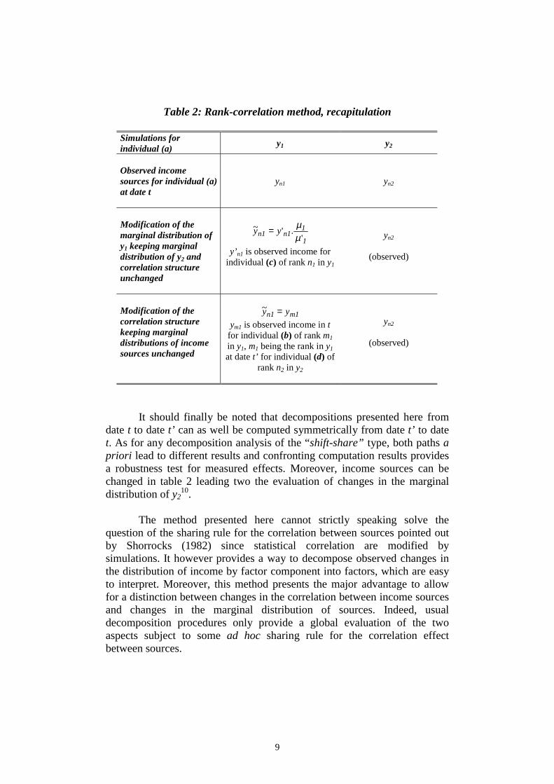
Following the notation described table 1, the two simulation proceduresdiscussed above can be summarised as follows for any individual (a):

9

Table 2: Rank-correlation method, recapitulation

Simulations forindividual (a) y1 y2

Observed incomesources for individual (a)at date t

yn1 yn2

Modification of themarginal distribution ofy1 keeping marginaldistribution of y2 andcorrelation structureunchanged

1

11n1n yy

'.'~µµ=

y’n1 is observed income forindividual (c) of rank n1 in y1

yn2

(observed)

Modification of thecorrelation structurekeeping marginaldistributions of incomesources unchanged

1m1n yy =~

ym1 is observed income in tfor individual (b) of rank m1in y1, m1 being the rank in y1at date t’ for individual (d) of

rank n2 in y2

yn2

(observed)

It should finally be noted that decompositions presented here fromdate t to date t’ can as well be computed symmetrically from date t’ to datet. As for any decomposition analysis of the “shift-share” type, both paths apriori lead to different results and confronting computation results providesa robustness test for measured effects. Moreover, income sources can bechanged in table 2 leading two the evaluation of changes in the marginaldistribution of y2

10.

The method presented here cannot strictly speaking solve thequestion of the sharing rule for the correlation between sources pointed outby Shorrocks (1982) since statistical correlation are modified bysimulations. It however provides a way to decompose observed changes inthe distribution of income by factor component into factors, which are easyto interpret. Moreover, this method presents the major advantage to allowfor a distinction between changes in the correlation between income sourcesand changes in the marginal distribution of sources. Indeed, usualdecomposition procedures only provide a global evaluation of the twoaspects subject to some ad hoc sharing rule for the correlation effectbetween sources.

10

A second major advantage of this method is that it allows for adecomposition of the whole distribution of income and is not based on aspecific inequality index. It thus allows for the decomposition of Lorenzcurves as well as any synthetic measure, every different index providingdifferent results depending on its specific sensitivity properties.

Finally, this method does not rely on any modelisation orparametrical assumption. It can nonetheless easily be combined with variousparameterisations in order to deal with related issues such as changes inlabour force participation or changes in household size.

Two main limits can however be noted here. First, the approachproposed can only provide a decomposition of changes in incomedistribution and does not give any static decomposition at a specific point intime as usual methods do. Second, the decomposition results do not providean exact decomposition of inequality changes and the sum of the variouseffects is not a priori equal to the total observed evolution11.

3. Taiwan 1979-94

This section provides an illustration of the rank-correlation methodto the evolution of household income distribution in Taiwan over the 1979-94 period.

3.1. Evolution of household income distribution in Taiwan (1979-94)

Taiwan appears as a counter-example to the Kuznets (1955)hypothesis predicting an inverted U-shape relationship between economicdevelopment and inequality. Indeed, since the settlement of the Republic ofChina in Taiwan in 1949, this country has experienced an exemplary growthprocess not only without increasing inequality but even with decreasingincome disparities up to the beginning of the 80s. This evolution has madeTaiwan in the 90s a newly industrialised country with high growth rates andinequality levels comparable or below western countries standards.

As shown figure 1, household income distribution has howeverbecome more unequal since the end of the 70s, which lead to a series ofdiscussions on what as been called, following Hung (1996), the “great U-turn”12.

11

Figure 1: Inequality of household income (1964-96)

(Gini)

0,27

0,28

0,29

0,3

0,31

0,32

0,33

64 69 74 79 84 89 94

Source: DGBAS (1996).

Inversely, the distribution of individual wages in Taiwan shows acontinuous decrease in inequality since the end of the 70s. The 80s and 90sthus appear as a period of divergence between a decrease in inequality at theindividual level and an increase in inequality in total household income.Using a micro-simulation based decomposition method, Bourguignon,Fournier and Gurgand (1999a) show that these trends come from thecombination of various compensating forces of strong magnitude. Indeed, astrong unequalising force, at the individual as well as at the household level,is shown to be caused by the rise in returns to education, whereas theexpansion of education in the population has had the opposite effect. Thisstudy shows that most of the observed divergence between the evolution inindividual and household income inequality is to be imputed to changes inhousehold structure. Other recent studies of the Taiwanese incomeinequality also emphasise changes in household structure as a key factor inexplaining the observed rise in household income inequality since the end ofthe 70s (Chu, 1997; Fields and Leary, 1997; Schultz, 1997; Tsai, 1994).Usual analyses of the decomposition of inequality changes as well as recentmethodological developments however fail to provide any further study ofthis phenomenon. The rank-correlation method exposed above thus appearshere as a valuable complementary tool for the identification of the sourcesof income inequality changes in Taiwan.

12

3.2. Data

Fully comparable micro-data from household survey are onlyavailable over the period 1979-94; we will thus restrict the analysis to theobserved rise in household income over this period.

The empirical analysis is based on a series of household surveysconducted annually since 1979 on samples composed of 16 400 householdsby the Taiwanese government (Directorate-General of Budget Accountingand Statistics, DGBAS). Household surveys are in fact available since 1976,but the quality of the data prior to 1979 as well as various adjustments madeon the size of the sample lead us to restrict the analysis to the period 1979onwards. The surveys are intended to provide information on the livingstandards of Taiwanese inhabitants and actually provide valuable, rich andreliable data13. A new sample is draws every year; it thus provides a set ofrepeated cross section and not a panel.

It should finally be noted that all income sources considered in thefollowing empirical work are evaluated as income per adult equivalent,using the square root of the total number of household members as theequivalence scale.

3.3. Changes in the structure of household income by type ofhousehold members

The joint evolution of household structure, participation behaviourand remuneration structure, which have been taking place in Taiwan overthe period studied has led to major changes in the structure of primaryhousehold income structure by type of household members. This evolutionis illustrated by the following table.

Tableau 3: Structure of primary household income by type of householdmembers (1979-94)

(%)Share in total income Share in wage income1979 1994 1979 1994

Wages Household head 49.5 50.1 69.2 65.7 Spouses 6.3 12.3 8.8 16.1 Children 8.0 5.1 11.2 6.7 Other members 7.7 8.7 10.8 11.4Income from independentactivities14 28.5 23.9 - -

It should first be noted that the share in total household wage incomeprovided by household heads has substantially declined, whereas that of

13

spouses increased quite strongly. Moreover, increasing scolarisation athigher education levels as well as the decline in fertility led to a strongdecrease in the relative share of children in total household income.

Changes in household structure also comes from changes in thecorrelation between the characteristics of household members, andespecially of spouses (Tsai, 1994). At the same time, changes inparticipation behaviour especially strong for spouses and children has alsoled to a modification of the correlation between individual incomes withinhouseholds15.

The following empirical work thus proposes an implementation ofthe rank-correlation method to total household income considered as thesum of individual income provided by various household members andincome derived from independent activities.

Changes in the marginal distribution of individual incomes ofdifferent household members

The first decomposition exercise proposed in the rank-correlationdecomposition method described above consists in isolating the specificimpact on total household income of observed changes in the distribution ofa specific income source. Figures 2 to 5 represent the specific effect ofchanges in the marginal distribution of the wage income of each type ofhousehold member. The effects are measured keeping the marginaldistribution of other income sources as well as rank-correlation between thesource studied and its complementary to total household income unchanged.Figures show the simulated variation in Lorenz curves. A negative curve onthe whole income scale corresponds to an increase in inequality (i.e. thedominance of Lorenz curves) induced by the simulation. Finally, asmentioned above, simulations are computed from initial to final date as wellas from final to initial date and the confrontation of both results can beviewed as a robustness test.

The plain curve represents the observed change in primaryhousehold income distribution as measured by Lorenz curves. Its negativesign up to the very top of the distribution reflects the observed rise ininequality described above using the Gini coefficient16.

These figures show that changes in the marginal distribution of alltypes of members except heads and children have had an equalising effecton overall household income distribution. The effect observed for householdheads is ambiguous, since curves cross the horizontal axis, whichcorresponds to a cross in Lorenz curves. However, the curves being firstabove and then below the horizontal axis, the effect is equalising at thebottom of the distribution and unequalising at the top. Lorenz dominance atthe bottom of the distribution implies that the measured effect will be

14

equalising for inequality indexes most sensitive to changes at the bottom ofthe distribution. As noted above, the distribution of individual income hasbecome more equal over the period studied, which naturally entails that thespecific effect of changes in the marginal distribution of most types ofhousehold members has had an equalising effect on total household incomedistribution.

Figures 2 to 5: Variation in the marginal distribution of wage income fordifferent household members

Variation in Lorenz curves – Household primary income (1979-94)Figure 2: Household heads

-0 ,01 5

-0 ,01

-0 ,00 5

0

0 ,00 5

0 20 40 60 80 100

Simulated variations

O bserved variation

Figure 3: Spouses

-0 ,01 5

-0 ,01

-0 ,00 5

0

0 ,00 5

0 ,01

0 20 40 60 80 100

Simulated variations

O bserved variation

Figure 4: Children

-0 ,01 5

-0 ,01

-0 ,00 5

0

0 ,00 5

0 20 40 60 80 100

Simulated variations

O bserved variation

Figure 5: Other members

-0 ,01 5

-0 ,01

-0 ,00 5

0

0 ,00 5

0 20 40 60 80 100

Simulated variations

O bserved variation

Note: Abscissas represent the cumulative share of households, ranked by increasing totalincome. The equivalence scale used is the square root of the total number of householdmembers. The number of household members weights households.

Results concerning children of household heads however call forfurther discussion. Indeed, the study of income distribution changes withinthis class also shows a decrease in inequality, however, figure 4 shows anon-ambiguous rise in inequality for total household income distributioninduced by this evolution. This result comes from the rapid widening ofscolarisation at higher levels, which led children to enter the labour marketmuch later. This evolution both comes from a strong concern and politicalefforts from the Taiwanese government17 as well as from a loosening of thebudget constraint for poorer households, induced by the high growth ratesobserved all over the period. As lower income households tend to have moreopportunities to keep their children scolarised for a longer period, theirrelative income in the whole population suffers all the more that childrenrepresent a much larger part of total household income at the bottom of thedistribution of household income. Applying the observed distribution ofchildren income in 1994 to the population observed in 1979 thus induces a

15

net loss coming from the increase in the share of non-working children,which is concentrated at the bottom of the distribution.

Changes in the correlation between the income of householdmembers

The second type of exercise proposed by the rank-decompositionmethod consists in measuring the specific impact of changes in thecorrelation between income sources, keeping marginal distribution ofsources unchanged. Figures 6 to 9 show the specific impact of changes inrank-correlation between the income of each type of household member andits complementary to total household income.

Figures 6 and 7 show non-ambiguous unequalising effects of strongmagnitude induced by changes in rank-correlation for household heads andspouses. These results can be related to two main simultaneous factors:rising female participation and rising endogamy in the assortative mating ofspouses especially in relation with education and age18 [Tsai (1994), Fieldsand Leary (1997)]. More specifically, concerning the rise in female laboursupply, Bourguignon, Fournier and Gurgand (1999a) show a sizeableunequalising effect induced both by entries into the labour force at the top ofthe distribution of household income and exits at the bottom. This evolutioncan be explained for one part by the rise in the participation of moreeducated women, which are strongly concentrated within richer household.For the other part, exits from the labour force of women belonging to poorerhouseholds can be explained as the result of a loosening of the budgetconstraint induced by the rapid rise in average income during the Taiwanesedevelopment process.

The specific impact of changes in the correlation between childrenincome and total household income shown figure 8 seems to go in the samedirection even though the effect depends on the sensitivity properties of theinequality index when computations are made upon the 1979 reference year.The central mechanism, as before, concerns the lengthening of scolarisation,which has had a stronger impact on children belonging to poorer householdsand which has been allowed by the overall rise in income. It is thus clearthat the decrease in labour force participation has increased, everything elsebeing equal, the correlation between household income and childrenincome, since more children have no income in poorer households. Figure 8isolates the effect keeping marginal distributions (and thus participation tothe labour market) unchanged and shows, at least for simulations based onthe 1994 data, a sizeable unequalising effect.

Finally, figure 9 shows a very similar trend (although non-robust)concerning the other members of the household. This evolution should belinked to the decrease in the age of retirement over the period studied.

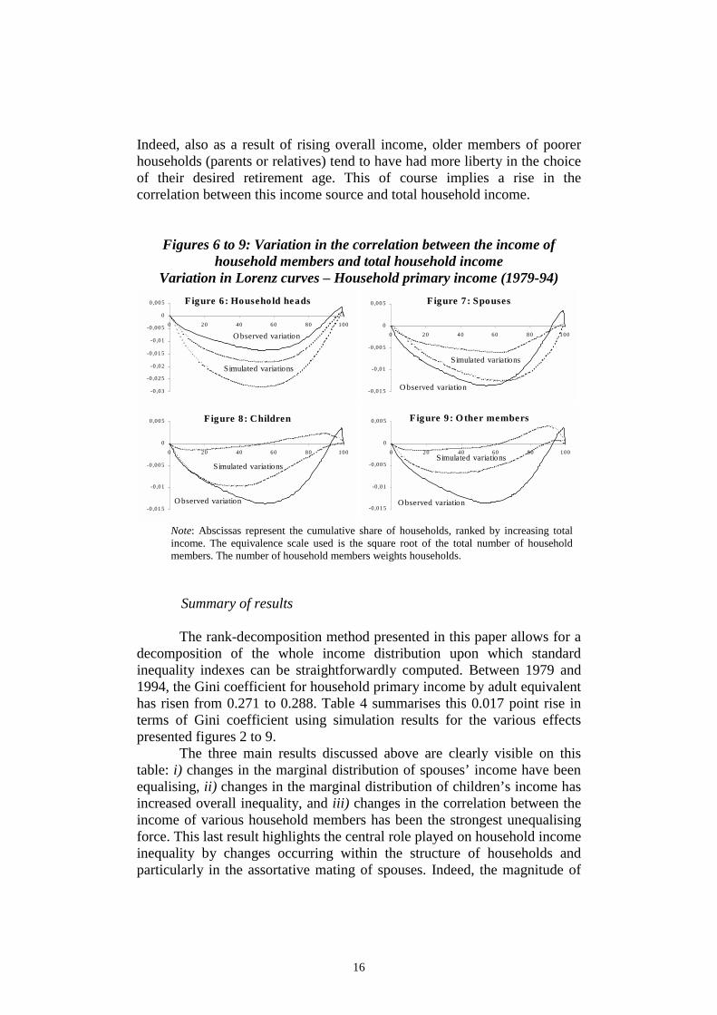
16

Indeed, also as a result of rising overall income, older members of poorerhouseholds (parents or relatives) tend to have had more liberty in the choiceof their desired retirement age. This of course implies a rise in thecorrelation between this income source and total household income.

Figures 6 to 9: Variation in the correlation between the income ofhousehold members and total household income

Variation in Lorenz curves – Household primary income (1979-94)Figure 6: Household heads

-0 ,03

-0 ,02 5

-0 ,02

-0 ,01 5

-0 ,01

-0 ,00 5

0

0 ,00 5

0 20 40 60 80 100

Simulated variations

O bserved variation

Figure 7: Spouses

-0 ,01 5

-0 ,01

-0 ,00 5

0

0 ,00 5

0 20 40 60 80 100

Simulated variations

O bserved variation

Figure 8: Children

-0 ,01 5

-0 ,01

-0 ,00 5

0

0 ,00 5

0 20 40 60 80 100

Simulated variations

O bserved variation

Figure 9: Other members

-0 ,01 5

-0 ,01

-0 ,00 5

0

0 ,00 5

0 20 40 60 80 100Simulated variations

O bserved variation

Note: Abscissas represent the cumulative share of households, ranked by increasing totalincome. The equivalence scale used is the square root of the total number of householdmembers. The number of household members weights households.

Summary of results

The rank-decomposition method presented in this paper allows for adecomposition of the whole income distribution upon which standardinequality indexes can be straightforwardly computed. Between 1979 and1994, the Gini coefficient for household primary income by adult equivalenthas risen from 0.271 to 0.288. Table 4 summarises this 0.017 point rise interms of Gini coefficient using simulation results for the various effectspresented figures 2 to 9.

The three main results discussed above are clearly visible on thistable: i) changes in the marginal distribution of spouses’ income have beenequalising, ii) changes in the marginal distribution of children’s income hasincreased overall inequality, and iii) changes in the correlation between theincome of various household members has been the strongest unequalisingforce. This last result highlights the central role played on household incomeinequality by changes occurring within the structure of households andparticularly in the assortative mating of spouses. Indeed, the magnitude of

17

the effect measured for household heads and spouses is comparable or largerthan the total observed change in inequality over the 1979-94 period.

Table 4: Summary of results using Gini coefficient (1979-94)

Gini Coefficient1979 Population* 1994 Population*

Observed variation 0.017

Variation due to marginal distributions Household head -0.001 -0.002 Spouses -0.007 -0.011 Children 0.009 0.003 Other members -0.002 -0.003

Variation due to correlation changes Household head 0.038 0.025 Spouses 0.016 0.008 Children 0.012 0.000 Other members 0.008 0.000

Notes: (*) Population upon which the simulation has been computed. The equivalence scaleused is the square root of the total number of household members. The number of householdmembers weights households.A negative number indicates a decrease in inequality. Different signs in the two columnscorrespond to a non-robust effect (for the Gini coefficient).

4. Conclusion

This article shows that the decomposition procedure briefly initiatedby Burtless (1999) can actually be systematised and provides a new generalmethod for decomposing income inequality changes by factor components.The method, based on the concept of rank-correlation, provides a useful toolanswering some major drawbacks inherent to usual decompositionprocedures.

Indeed, this method allows for a decomposition of the whole incomedistribution and is thus not restricted to the use of a specific inequalityindex. It thus provides a decomposition procedure for observed changes inLorenz curves as well as any synthetic inequality measure and the resultsobtained depend on the specific sensitivity properties of chosen indexes atvarious points of the distribution, which is not the case for decompositionmethods following Shorrocks (1982) approach.

18

Moreover, the decomposition procedure proposed here providesuseful answers to the central question raised by Shorrocks (1982) about thesharing of the role played by the correlation between sources among incomesources. The rank-decomposition method indeed allows for a furtherdecomposition step in distinguishing the specific impact of changes in thecorrelation between sources from that of changes in the marginaldistribution of sources, whereas usual decomposition procedures onlyprovide a global evaluation based on a given sharing rule for correlationfactors, which is inevitably partial.

The implementation of the method to the Taiwan case illustrates thetype of results it can provide and allows for a better understanding of somemajor factors behind the rise in household income inequality over the 1979-94 period. Indeed, three main sources of inequality change can be derivedfrom this decomposition procedure: i) a sizeable equalising effect comingfrom changes in the distribution of spouses’ (marginal) income distribution,ii) a notable unequalising effect induced by the decline in labour forceparticipation of children following the rise in scolarisation, and iii) a majorunequalising effect (which magnitude is much stronger than the first two)coming from changes in the correlation between various householdmembers’ income. We finally argue here, that this last point is to be linkedwith changes in the assortative mating of spouses and especially with risingendogamy in terms of education and age induced by profound sociologicalchanges leading to a shift from traditional Chinese marriages to a freerchoice of bride or groom.

Results for the Taiwanese case plead more generally in favour of theuse and development of methods dealing with inequality decomposition byfactor components. Indeed, the method proposed here is complementary torecent developments in inequality decomposition through micro-simulationtechniques (Juhn, Murphy and Pierce, 1993; Bourguignon and Martinez,1997; Bourguignon, Fournier and Gurgand, 1999a)19. These methods onlyprovide a general evaluation of the impact of changes in population andhousehold structure on income distribution and can not isolate the specificfactors highlighted here. Combining both approaches within a commonframework would certainly be of great interest for the understanding of themajor sources of inequality changes.

19

References

ATKINSON A. B. (1997), « Bringing Income Distribution in from the Cold »,Economic Journal, n° 107, pp. 297-321.

ATKINSON A. B. and F. BOURGUIGNON (1998), Introduction to Handbook ofIncome Distribution, North Holland, forthcoming.

BOURGUIGNON F., M. FOURNIER and M. GURGAND (1999a), « Fastdevelopment with a Stable Income Distribution: Taiwan, 1979-1994 »,Document de travail Crest n° 9921.

BOURGUIGNON F., M. FOURNIER and M. GURGAND (1999b), « FemaleLabour Supply in the Course of Taiwan’s Economic Development:1979-94 », Document de travail Crest n° 9920.

BOURGUIGNON F. and M. MARTINEZ (1997), « Decomposition of thechanges in the distribution of primary family income: a microsimulationapproach applied to France, 1979-1989 », Document de travail Delta,Paris.

BURTLESS G. (1999), « Effects of growing wage disparities and changingfamily composition on the U.S. income distribution », EuropeanEconomic Review, April, Vol. 43, pp. 853-65.

CHANTREUIL F. and A. TRANNOY (1997), « Inequality DecompositionValues », Mimeo, THEMA, Université de Cergy-Pontoise.

CHU Y. P. (1997), « Employment Expansion and Equitable Growth :Taiwan’s Post-war Experience », Mimeo Academia Sinica, Taipei.

DEATON A. and C. PAXSON (1993), « Saving, growth and aging inTaiwan », NBER Working Paper No. 4330.

DINARDO J., N. FORTIN and T. LEMIEUX (1996), « Labour market institutions andthe distribution of wages 1973-1992: A semiparametric approach »,Econometrica, Vol. 64, September, pp. 1001-1064.

DIRECTORATE GENERAL OF BUDGET, ACCOUNTING AND STATISTICS (1996),Report on the Survey of Family Income and Expenditure in Taiwan Areaof Republic of China, Executive Yuan, Republic of China.

FEI J., G. RANIS and S. KUO (1978), « Growth and the Family Distributionof Income by Factor Component », Quarterly Journal of Economics,February, pp. 17-54.

FIELDS G. S. and J. LEARY (1997), « Economic and demographic aspects ofTaiwan’s rising family income inequality », Mimeo.

FOURNIER M. (1999), Développement et distribution des revenus : Analysespar décomposition de l’expérience taiwanaise, PhD thesis, EHESS,Paris.

GOTTSCHALK, R. and S. DANZIGER (1993), « Family structure, family size,and family income: accounting for changes in the economic well-beingof children, 1968-1986 », in S. DANZIGER and GOTTSCHALK, R. (eds.),Uneven Tides: Rising Inequality in America. New York: Russel Sagefoundation.

20

HUNG R (1996), « The Great U-Turn in Taiwan: Economic Restructuringand a Surge in Inequality », Journal of Contemporary Asia, Vol. 26, No.2, pp. 151-163.

JUHN C., K. MURPHY and B. PIERCE (1993), « Wage Inequality and the Risein Returns to Skill », Journal of Political Economy, Vol. 101, No. 3, pp.410-442.

KANBUR R. and N. LUSTIG (1999), « Why is Inequality Back on theAgenda? », Paper prepared for the Annual Bank Conference onDevelopment Economics, Washington, D.C., 28-30 April 1999.

KUZNETS S. (1955), « Economics growth and income inequality »,American Economic Review, Vol. 45, pp. 1-28.

LERMAN R. I. (1996), « The Impact of the Changing US Family Structure onChild Poverty and Income Inequality », Economica, Vol. 63, pp. S119-S139.

PYATT G., C. N. CHEN and J. FEI (1980), « The Distribution of Income byFactor Components », Quarterly Journal of Economics, Vol. 95,Novembre, pp. 451-473.

SCHULTZ T. P. (1997), « Income Inequality in Taiwan 1976-1995: ChangingFamily Composition, Aging and Female Labour-Force Participation »,Economic Growth Center Discussion Paper, No. 778, Yale University.

SHORROCKS A. F. (1982), « Inequality Decomposition by FactorComponents », Econometrica, Vol. 50, No. 1, January, pp. 193-211.

TSAI S. L. (1994), « Assortative Mating in Taiwan », in S. K. Lau, M. K.Lee, P. S. Wan and S. L. Wong (eds.), Inequalities and Development,Hong Kong Institute of Asia-Pacific Studies, The Chinese University ofHong Kong.

21

Appendix 1 Conditions proposed by Shorrocks (1982)

Shorrocks (1982) proposes the following six conditions for thedecomposition of total income Y by N factor components:

- Condition 1: I is a continuous and symmetric inequality measure.

- Condition 2 (Continuity and symmetry):

a) Each term NkkS ...1, = is continuous in Yk.b) Terms NkkS ...1, = are invariant to any permutation of income

sources.

- Condition 3 (Independence of the level of disaggregation): Eachcomponent NkkS ...1, = is independent of how other factors Yj!k aregrouped.

- Condition 4 (Consistence of the decomposition): NkkS ...1, = is

invariant to any permutation of individuals1.

- Condition 5 (Normalisation): The contribution of an evenlydistributed income source is 0.

- Condition 6 (Symmetry): For any two factor componentsdecomposition (Y1 and Y2), if Y1 can be derived from Y2 by asimple permutation then S1 = S2.

1 The term “individual” is to be understood here as any unit(individual, household, family, etc.).

22

Appendix 2 Example of implementation of the rank-decompositionmethod

Distributions of income sources at dates t and t’:

Date t Date t’Income

y1

Rank /y1

Incomey2

Rank /y2

y =y1+y2

Incomey1

Rank /y1

Incomey2

Rank /y2

y =y1+y2

10 2 5 1 15 15 3 10 1 255 1 15 2 20 13 2 15 2 28

25 3 30 3 55 12 1 25 3 37

Modification of marginal distribution of income source y2 keeping marginaldistributions of other income sources and correlation between sources

unchanged:

Income1y~

Rank /1y~

Incomey2

Rank /y2

y~ =

1y~ + y’.213 2 5 1 1812 1 15 2 2715 3 30 3 45

Modification of correlation between sources keeping marginaldistributions of sources unchanged:

Income1y~

Rank /1y~

Incomey2

Rank /y2

y~ =

1y~ + y’.225 3 5 1 3010 2 15 2 255 1 30 3 35

23

Notes

1 Developments of the micro-simulation methodology proposed by Bourguignon, Fournierand Gurgand (1999) however take into account some aspects of the question, modellingspecifically occupational choice behaviours and income functions in various occupations.2 Total household can indeed be considered as the sum of individual incomes of varioushousehold members.3 See for example Burtless (1999), Gottschalk and Danziger (1993) and Lerman (1996).4 Shorrocks (1982) calls it the "natural decomposition".5 This drawback has led various authors to relax some of Shorrocks (1982) axioms. See forexample Chantreuil and Trannoy (1997).6 The term “individual” is to be understood here as any unit (individual, household, family,etc.).7 Counter-factual incomes imputed have to be weighted by the share of the mean of theincome source at dates t and t’ in order to preserve the overall mean income observed in t.8 The generalisation to three sources and more is straightforward.9 Here again, the statistical correlation simulated will not a priori correspond to that of datet’.10 The effect measured for the modification of the correlation between income sources ishowever unchanged whatever income source the simulation is based upon.11 It would be possible to provide an exact decomposition by computing various simulationsbased on the previous estimation results. This type of decomposition would however lead toan important number of possible combinations concerning the order in which simulationmay be computed, each combination giving a priori a different result.12 This result, illustrated here on gross total household income is robust to the use of variousequivalence scales (Fournier, 1999, pp.222-224).13 For a discussion on the reliability of the data, see for example Deaton and Paxson (1993).14 Income derived from independent activities of household members (agricultural or not)can not be affected to any particular household member in the data.15 For a detailed study of changes in female labour supply in Taiwan over the 1979-94period, see Bourguignon, Fournier and Gurgand (1999b).16 Fournier (1999) shows that most inequality indicators show a rise in inequality.17 Free and compulsory education has been lengthened from 6 to 9 years in 1968 and a lawhas recently been passed to implement a further increase to 12 years by 2001.18 The correlation coefficient between the education of spouses rose from 0.66 to 0.72between 1979 and 1994. Between the age of spouses, a rise from 0.84 to 0,90 has beentaking place over the same period.19 See Fournier (1999) for a detailed presentation of the methodology.