inequality in the twenty-first century economic theory ... · 1 inequality in the twenty-first...
TRANSCRIPT
1
Inequality in the Twenty-First Century – Economic Theory Revisited
Hanna Szymborska
University of Leeds1
Abstract
This paper argues that analyses of inequality based on existing theories of
distribution do not adequately account for growing wealth disparities. This is
because the division into capitalists and workers traditionally envisaged in the
Post Keynesian wage share models has been altered by financialisation, making
these categories more heterogeneous. Financial deregulation and securitisation
have contributed to the falling wage share of national income. The rich
accumulate high-yielding assets while the middle/low-income groups suffer
from high leverage due to unsustainable debt accumulation. Rising indebtedness,
linked to stagnating wage growth and validated by the growing demand for
asset-backed securities among financial investors, has led to massive wealth
disparities. Recent contributions to the stock flow consistent modelling literature
incorporate some wealth considerations into the Post Keynesian stock flow
consistent models by distinguishing between rentiers, non-managerial and
managerial workers as well as by allowing for indebtedness of non-supervisory
workers and consumption emulation. This paper aims to complement these
contributions by focusing on how financialisation has altered the structures of
households’ balance sheets, and affected their stability. In particular, the
implications of these changes for income distribution are examined in a stock
flow consistent model of a US economy with three classes of households and a
complex financial sector. The simulation results reveal that balance sheet
heterogeneity among households has an important impact on inequality levels.
WORK IN PROGRESS – DO NOT QUOTE
Note
The author wishes to thank Yannis Dafermos, Gary Dymski, Antoine Godin, Maria
Nikolaidi, Ozlem Onaran and Cem Oyvat for comments on an earlier draft of the paper.
1 Contact e-mail: [email protected]
1
Table of Contents
I. Introduction ......................................................................................................................... 2
II. Theories of inequality and the conceptualisation of the middle class ....... 10
III. Wealth and inequality in stock-flow consistent models .................................. 16
IV. Model specification ........................................................................................................ 17
The household sector .............................................................................................................................. 20 Firms .............................................................................................................................................................. 29 Commercial banks .................................................................................................................................... 30 SPVs/underwriters .................................................................................................................................. 32 Institutional investors ............................................................................................................................ 32 Simulations ................................................................................................................................................. 33
V. Results ................................................................................................................................. 35
VI. Conclusion and future work ....................................................................................... 42
References ....................................................................................................................................... 46
Appendix .......................................................................................................................................... 52
List of Figures
Figure 1. Change in homeownership rate by percentile, USA 1989-2012................. 4
Figure 2. The top 1% income share, USA 1980-2013 ........................................................ 5
Figure 3. Mean and median net worth, the mean-median ratio, USA 1983-2013 .. 6
Figure 4. Financial fragility measures by percentile, USA 2010 .................................... 7
Figure 5. Median net worth annual growth rate by decile, USA 1989-2013 ............ 8
Figure 6. Household portfolio composition, USA 2014 ..................................................... 9
Figure 7. Simulation results – full model ............................................................................. 35
Figure 8. Simulation results – “pure capitalists” specification .................................... 39
Figure 9. Simulation results – “pure capitalist” specification, no rentier debt ..... 40
Figure 10. Simulation results – reduced specification without securitisation ..... 41
List of Tables
Table 1. Annual growth rate of average hourly wages, USA 1979-2012 ................. 12
Table 2. Balance sheet matrix .................................................................................................. 18
Table 3. Transaction flow matrix ............................................................................................ 19
2
I. Introduction
The main goal of this paper is to examine the dynamics of income and wealth
inequality in high-income countries and the implications for the stability of
household financial positions across the distribution in the light of financial
sector transformation since 1980s. A theoretical stock flow consistent model is
proposed, aiming to explain the concentration of income and wealth at the top of
the distribution and the diffusion of financial fragility to the rest of the society.
The innovation of the model lies in its interpretation of inequality as balance
sheet structure disparities, based on a reinterpretation of the working and
rentier class and a new conceptualisation of the middle class in Post Keynesian
analysis. Three-class specification of the household sector is developed,
accounting for indebtedness, financial fragility and wage inequality – processes
strongly associated with the impact of financial sector transformation on
inequality.
Financial sector transformation, often described by the umbrella term
“financialisation”, is an extremely complex process occurring at a variety of
dimensions. Although most pronounced in USA, it has also taken place in various
aspects and at different points since 1980s in Europe (cf. Pasarella Veronese
2013).
Financialisation finds its roots in the persistently high inflation and high
interest rates in the late 1960s, which induced non-financial companies to turn
to financial markets rather than banks for investment financing. This realigned
firms’ objectives away from long-term investment towards short-term
profitability, making them more involved in financial activities (such as issuing
shares), which raised the importance of financial over real profits and
contributed to the growing share of the financial, insurance and real estate
sector (FIRE) in the economy at the expense of manufacturing (Palley 2007:18).
The processes of financialisation gained steam in the 1980s under policies
promoting market liberalisation and retrenchment of the state from public
service provision associated with the leadership of Reagan in USA and Thatcher
in UK (Sawyer 2013:13). Firstly, labour market liberalisation and the associated
3
rolling back of minimum wage, unemployment protection and union-oriented
policies resulted in gradually declining wage income growth. Simultaneously,
provision of pensions, housing and public goods such as education and
healthcare was increasingly delegated from the state to the private sector. With
stagnant wages and diminishing state provision, households found themselves in
need of additional financing through borrowing.
Rising credit demand was paralleled by the massive proliferation of
financial instruments and the development of structured finance. The
aforementioned turn of non-financial companies towards financial markets
resulting from high borrowing costs in 1960s and 70s led financial
intermediaries to seek revenue in the household sector and through innovation
of new financial products (Dymski 2009:157). An increasing volume of financial
obligations — primarily consumer debt and mortgages — was transformed into
securities in a process labelled securitisation, forming collateralised debt
obligations (CDOs), which combined financial instruments of varying risk and
return characteristics (Pollin/Heintz 2013:113). The establishment of credit
default swaps (CDS) and derivatives on existing products allowed investors to
bet against the default of any financial instrument, leading to the transformation
of traditional lending relations based on intermediation towards an “originate
and redistribute" model, where default risk became “originated" by creditors and
then spread across the financial system through securitisation. The actors of this
new lending model were not only registered banks, transformed into highly
consolidated “megabanks” as a result of intense merger activity, but also non-
bank intermediaries, which played a role similar to that of formal banks but were
outside central bank’s jurisdiction in obtaining liquidity (ibid.:115). This whole
process was validated by increasing financial deregulation measures such as the
Gramm-Leach-Bliley Act in 1999 in USA, which allowed commercial banks to
engage in financial investment activities.
The combination of demand factors (stagnant earnings, privatisation of
public services) and supply factors (securitisation, deregulation) led households
in high-income economies to become more involved in financial markets,
although to a varying extent in different countries depending on the degree of
4
liberalisation and deregulation introduced. On the supply side, financial
intermediaries were eager to include more households in their services partly to
compensate for diminishing deposits from non-financial firms (banks) and partly
to generate more underlying assets for CDOs so as to keep pace with the rapidly
growing demand for securitised instruments among financial investors (bank
and non-bank intermediaries) (cf. Goda/Lysandrou 2013). In the process, many
non-bank intermediaries took advantage of lax financial regulation and engaged
in predatory lending practices by offering “subprime" mortgages at extremely
harsh conditions to social groups previously excluded from access to credit, such
as the young, women and racial minorities (cf. Dymski et al. 2013). Those
subprime mortgages formed a lion share of securitised assets demanded by
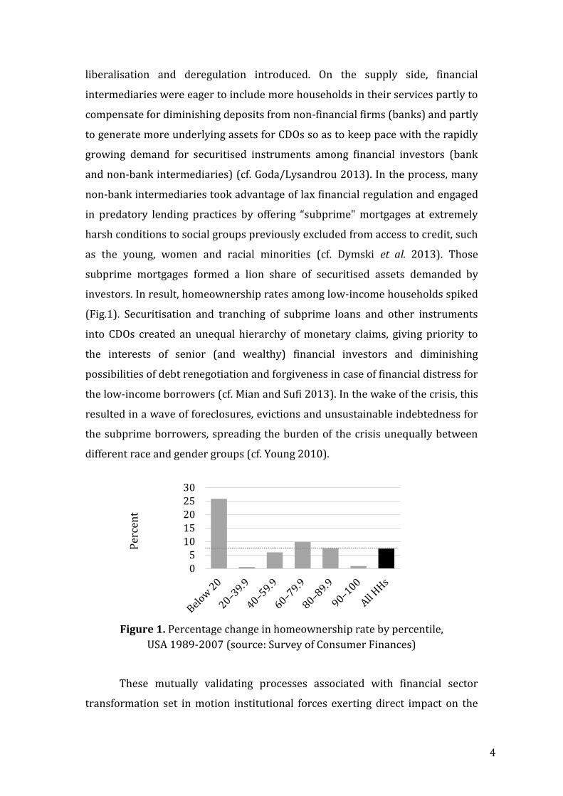
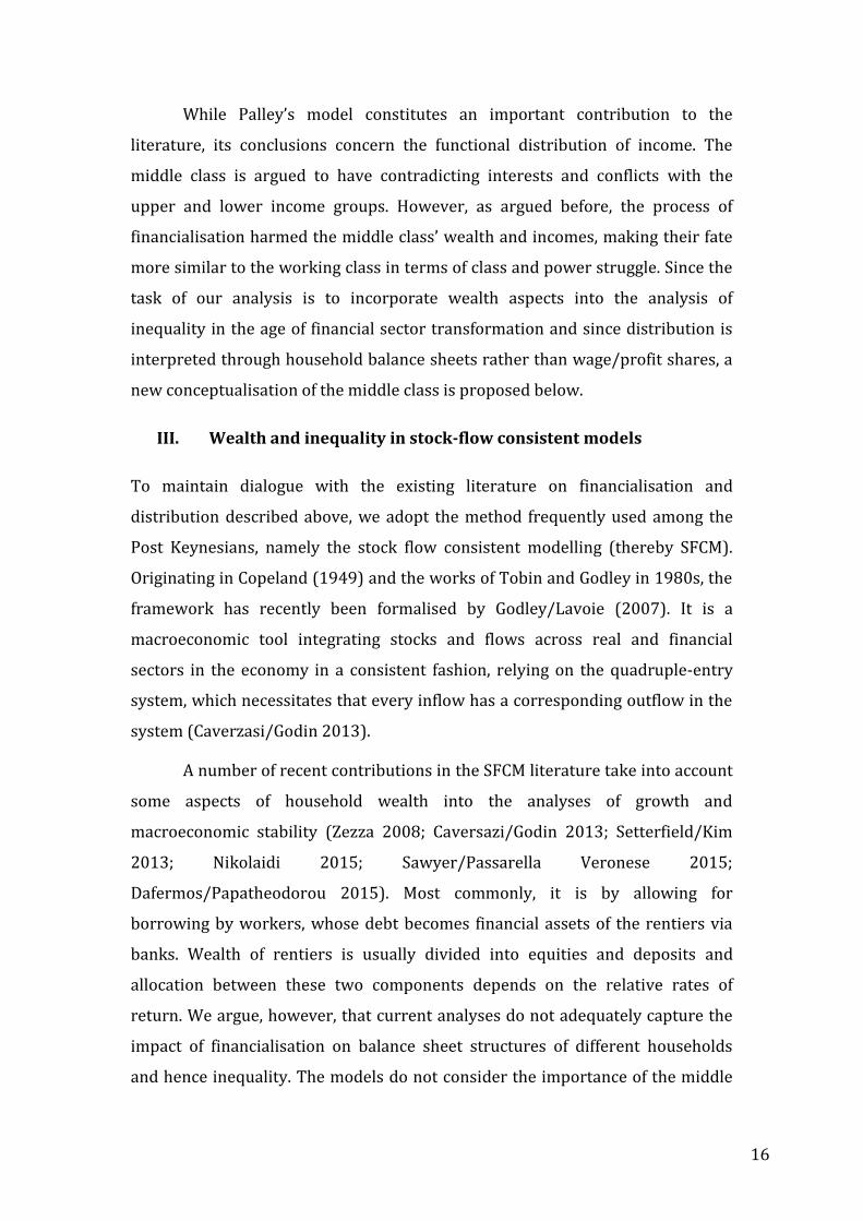
investors. In result, homeownership rates among low-income households spiked
(Fig.1). Securitisation and tranching of subprime loans and other instruments
into CDOs created an unequal hierarchy of monetary claims, giving priority to
the interests of senior (and wealthy) financial investors and diminishing
possibilities of debt renegotiation and forgiveness in case of financial distress for
the low-income borrowers (cf. Mian and Sufi 2013). In the wake of the crisis, this
resulted in a wave of foreclosures, evictions and unsustainable indebtedness for
the subprime borrowers, spreading the burden of the crisis unequally between
different race and gender groups (cf. Young 2010).
Figure 1. Percentage change in homeownership rate by percentile,
USA 1989-2007 (source: Survey of Consumer Finances)
These mutually validating processes associated with financial sector
transformation set in motion institutional forces exerting direct impact on the
05
1015202530
Per
cen
t
5
dynamics of income and wealth distribution in advanced countries. Data show
that various measures of inequality have dramatically increased in high-income
countries. In USA, where the trends are the most extreme, Gini coefficient for
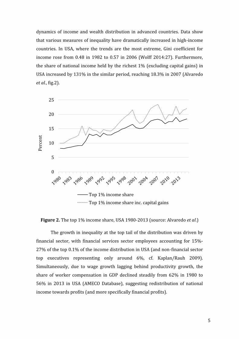
income rose from 0.48 in 1982 to 0.57 in 2006 (Wolff 2014:27). Furthermore,
the share of national income held by the richest 1% (excluding capital gains) in
USA increased by 131% in the similar period, reaching 18.3% in 2007 (Alvaredo
et al., fig.2).
Figure 2. The top 1% income share, USA 1980-2013 (source: Alvaredo et al.)
The growth in inequality at the top tail of the distribution was driven by
financial sector, with financial services sector employees accounting for 15%-
27% of the top 0.1% of the income distribution in USA (and non-financial sector
top executives representing only around 6%, cf. Kaplan/Rauh 2009).
Simultaneously, due to wage growth lagging behind productivity growth, the
share of worker compensation in GDP declined steadily from 62% in 1980 to
56% in 2013 in USA (AMECO Database), suggesting redistribution of national
income towards profits (and more specifically financial profits).
Per
cen
t
0
5
10
15
20
25
Top 1% income share
Top 1% income share inc. capital gains
6
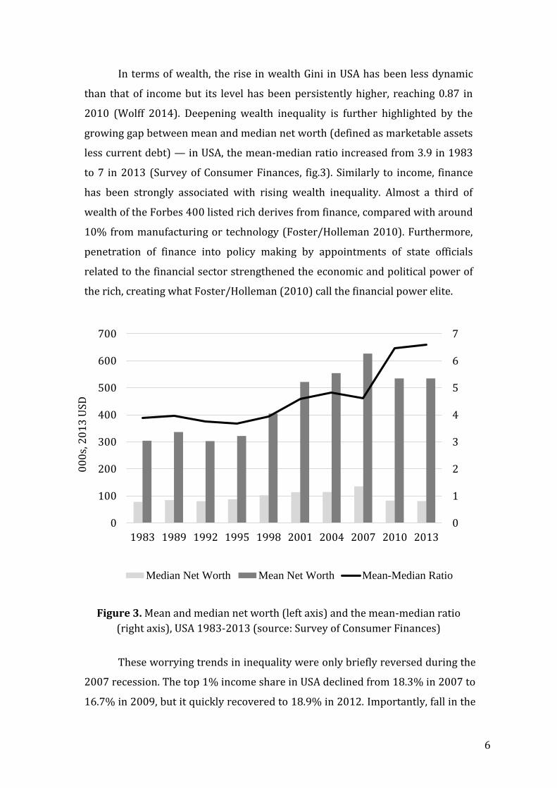
In terms of wealth, the rise in wealth Gini in USA has been less dynamic
than that of income but its level has been persistently higher, reaching 0.87 in
2010 (Wolff 2014). Deepening wealth inequality is further highlighted by the
growing gap between mean and median net worth (defined as marketable assets
less current debt) — in USA, the mean-median ratio increased from 3.9 in 1983
to 7 in 2013 (Survey of Consumer Finances, fig.3). Similarly to income, finance
has been strongly associated with rising wealth inequality. Almost a third of
wealth of the Forbes 400 listed rich derives from finance, compared with around
10% from manufacturing or technology (Foster/Holleman 2010). Furthermore,
penetration of finance into policy making by appointments of state officials
related to the financial sector strengthened the economic and political power of
the rich, creating what Foster/Holleman (2010) call the financial power elite.
Figure 3. Mean and median net worth (left axis) and the mean-median ratio
(right axis), USA 1983-2013 (source: Survey of Consumer Finances)
These worrying trends in inequality were only briefly reversed during the
2007 recession. The top 1% income share in USA declined from 18.3% in 2007 to
16.7% in 2009, but it quickly recovered to 18.9% in 2012. Importantly, fall in the
0
1
2
3
4
5
6
7
0
100
200
300
400
500
600
700
1983 1989 1992 1995 1998 2001 2004 2007 2010 2013
Median Net Worth Mean Net Worth Mean-Median Ratio
00
0s,
20
13
US
D
7
3.5
60.6
18.921
127
41.2
71.5
134.5
51.3
0
20
40
60
80
100
120
140
Debt / equity ratio Debt / income ratio Principal residencedebt / house value
Top 1%
All HHs
Middle 3
quintiles
top 1% share of national income was redistributed within the top quintile, as the
share of the top 10% decreased by far less than the top 1% share between
2007-2011 (Dufour/Orhangazi 2016:165). Real wages were temporarily on the
rise and despite growing unemployment, low and middle income households
suffered smaller income losses than the top 1%. The latter saw they capital
income diminished in result of falling asset and property prices
(Dufour/Orhangazi 2016:165). The overall Gini coefficient for income fell from
0.57 to 0.55 (Wolff 2014:27). Nevertheless, there are reasons to believe that the
relative income gains for the working class are likely to be short lived as positive
growth of real wages in recent years has been driven primarily by low inflation
(caused mainly by falling commodity prices, which are known to be highly
volatile) rather than rising nominal wages (Gould 2016).
In contrast, while falling asset prices slightly diminished the stocks of
wealth of the rich, the Gini coefficient for wealth increased by 0.035 Gini points
in the post-crisis period (Wolff 2014:32). In fact, while median net wealth fell by
21.2% from 2007 to 2010, mean net wealth saw only 6.5% decline, suggesting an
uneven burden of the crisis across the society (ibid.:24). The increase in wealth
inequality during the crisis was due to different degrees of leverage across the
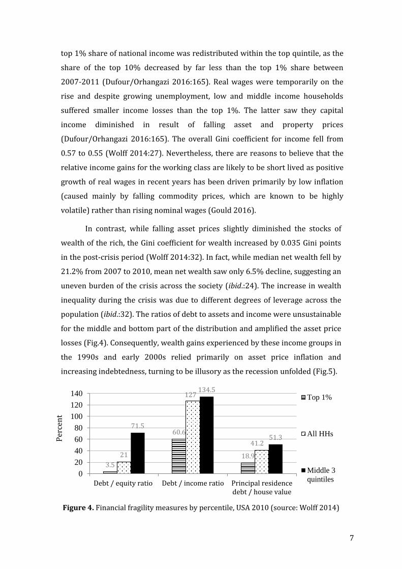
population (ibid.:32). The ratios of debt to assets and income were unsustainable
for the middle and bottom part of the distribution and amplified the asset price
losses (Fig.4). Consequently, wealth gains experienced by these income groups in
the 1990s and early 2000s relied primarily on asset price inflation and
increasing indebtedness, turning to be illusory as the recession unfolded (Fig.5).
Figure 4. Financial fragility measures by percentile, USA 2010 (source: Wolff 2014)
Per
cen
t
8
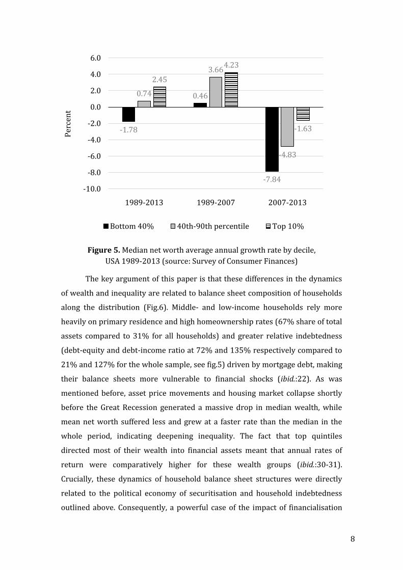
Figure 5. Median net worth average annual growth rate by decile,
USA 1989-2013 (source: Survey of Consumer Finances)
The key argument of this paper is that these differences in the dynamics
of wealth and inequality are related to balance sheet composition of households
along the distribution (Fig.6). Middle- and low-income households rely more
heavily on primary residence and high homeownership rates (67% share of total
assets compared to 31% for all households) and greater relative indebtedness
(debt-equity and debt-income ratio at 72% and 135% respectively compared to
21% and 127% for the whole sample, see fig.5) driven by mortgage debt, making
their balance sheets more vulnerable to financial shocks (ibid.:22). As was
mentioned before, asset price movements and housing market collapse shortly
before the Great Recession generated a massive drop in median wealth, while
mean net worth suffered less and grew at a faster rate than the median in the
whole period, indicating deepening inequality. The fact that top quintiles
directed most of their wealth into financial assets meant that annual rates of
return were comparatively higher for these wealth groups (ibid.:30-31).
Crucially, these dynamics of household balance sheet structures were directly
related to the political economy of securitisation and household indebtedness
outlined above. Consequently, a powerful case of the impact of financialisation
Per
cen
t
-1.78
0.46
-7.84
0.74
3.66
-4.83
2.45
4.23
-1.63
-10.0
-8.0
-6.0
-4.0
-2.0
0.0
2.0
4.0
6.0
1989-2013 1989-2007 2007-2013
Bottom 40% 40th-90th percentile Top 10%
9
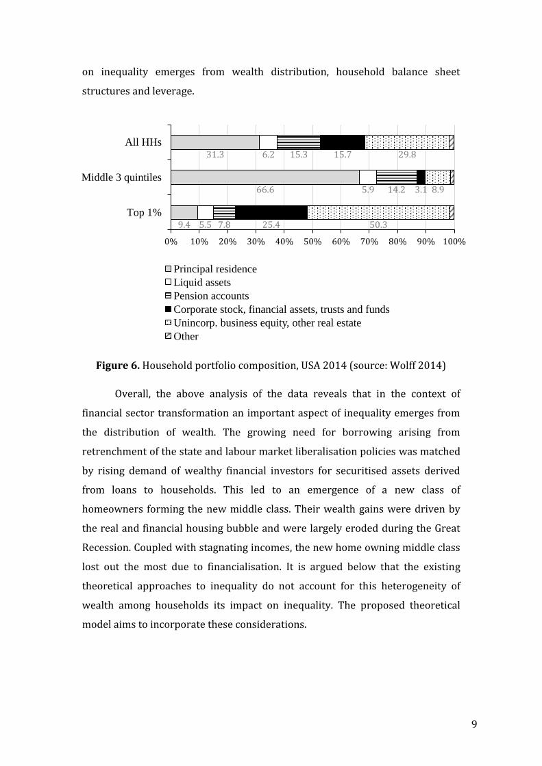
on inequality emerges from wealth distribution, household balance sheet
structures and leverage.
Figure 6. Household portfolio composition, USA 2014 (source: Wolff 2014)
Overall, the above analysis of the data reveals that in the context of
financial sector transformation an important aspect of inequality emerges from
the distribution of wealth. The growing need for borrowing arising from
retrenchment of the state and labour market liberalisation policies was matched
by rising demand of wealthy financial investors for securitised assets derived
from loans to households. This led to an emergence of a new class of
homeowners forming the new middle class. Their wealth gains were driven by
the real and financial housing bubble and were largely eroded during the Great
Recession. Coupled with stagnating incomes, the new home owning middle class
lost out the most due to financialisation. It is argued below that the existing
theoretical approaches to inequality do not account for this heterogeneity of
wealth among households its impact on inequality. The proposed theoretical
model aims to incorporate these considerations.
9.4
66.6
31.3
5.5
5.9
6.2
7.8
14.2
15.3
25.4
3.1
15.7
50.3
8.9
29.8
0% 10% 20% 30% 40% 50% 60% 70% 80% 90% 100%
Top 1%
Middle 3 quintiles
All HHs
Principal residence
Liquid assets
Pension accounts
Corporate stock, financial assets, trusts and funds
Unincorp. business equity, other real estate
Other
10
II. Theories of inequality and the conceptualisation of the middle
class
Despite its importance in inequality dynamics described above, middle class as
an analytical category has been neglected in the existing theories of inequality.
Although aspects of wealth have been increasingly incorporated into
distributional theories, heterogeneity of households financial positions has not
been taken into consideration explicitly.
Theory putting the largest emphasis on the importance of wealth for
inequality is found in the seminal work of Piketty (2014). The main premise of
his “Capital in the Twenty-First Century” is that inequality is driven by
accumulation of persistently higher returns to wealth (r) relative to the growth
of income (g) (historically averaging at 5% and 1% respectively). Compounding
of the returns to wealth overtime generates higher income flows for the wealth
holders and their inheritors (identified with the top 0.1-1%) than for the rest of
the society. Higher capital income in turn allows for greater saving, facilitating
further wealth generation and perpetuating inequality. In other work
(Piketty/Zucman 2014) it is emphasised that due to its high concentration and
the aforementioned accumulation dynamics, inequality of wealth is more
important for the overall structure of inequality in the 21st century than in the
post-war era. Importantly, saving and consumption propensities are not enough
to predict wealth-income levels in advanced countries (higher wealth-income
ratios suggesting large economic power of asset holders and deepening
inequality). This is because capital gains (often driven by housing wealth) are
found to account for around 40% of increase in national wealth to income ratios
between 1970 and 2010 (Piketty/Zucman 2014:1288).
Piketty’s insight regarding the interplay between income and wealth
dynamics and its impact on inequality is particularly relevant in the age of
financialisation. As highlighted in the introduction, financial innovation and
securitisation influenced inequality by generating differential rates of return and
degrees of volatility across the distribution. Large wealth holdings of the rich
allowed them to invest in high-yielding financial instruments (often requiring
large initial payments, which can only be afforded at high levels of net worth),
11
generating sizeable capital income. Moreover, they were able to use their
economic power to secure higher wages, particularly when employed in financial
sector.
Despite the importance of its general conclusions, Piketty’s “Capital in the
Twenty-First century” suffers from several drawbacks. The most relevant
criticisms for our analysis concern the weakness of Piketty’s theoretical
explanation and insufficient emphasis on household debt in contributing to
inequality.
While his empirical work is to be applauded, theoretical explanation for
inequality based on “r greater than g” relies on the expectation that these trends
observed in the past would continue into the future (Pressman 2016:159).
Hence, Piketty does not provide any explicit theoretical explanation why returns
to wealth should always exceed the growth of income. Consequently, despite the
relevance of his conclusions, there is no formal link between inequality and
financial sector transformation in Piketty’s framework.
The alternative body of theoretical literature identified with the Post
Keynesian functional distribution explicitly takes into account the link between
financialisation and distribution. It focuses on the macroeconomic impact of
increasingly unequal functional distribution of national income between two
factors of production – capital and labour – which are associated with higher
propensity to save and consume respectively (cf. Kalecki 1971). The distributive
forces of financialisation are seen as the maximisation of shareholder value,
proxied by a higher rentier (i.e. capitalist) income share, although the precise
view on which of the aspects of financialisation is the most important for
redistribution varies among researchers (cf. Hein 2009, 2015; Hein/Van Treeck
2010; Palley 2012, 2013; Van Treeck 2009). These models often draw from
Bhaduri/Marglin (1990) argument that the macroeconomic effects of income
transfers between wage and profit earners hinge on whether the economy is
wage- or profit-led. Onaran et al. (2011) establish that the majority of advanced
economies are wage-led, which in the Bhaduri/Marglin framework signifies that
lower wage share resulting from financial sector transformation has a negative
impact on aggregate demand and growth by undercutting effective investment
12
demand because resources are taken away from those who are more likely to
spend them to those who are more likely to hoard them.
However, what this theoretical approach has not yet done is to examine
how the transformation in the nature of financial intermediation has
complexified the division of society into two distinct categories. Both groups of
“workers” and “capitalists” have become heterogeneous, which complicates their
analytical usefulness. In the course of financialisation workers became the
recipients of capital income through homeownership and private pension
schemes, while capitalists became the recipients of the highest wages in the
economy. In fact, the top 10% of earners were the only income group with
above-average income growth between 1979-2012 (Bivens et al. 2014), with the
top 5% of wage earners experiencing a wage increase during the Great Recession
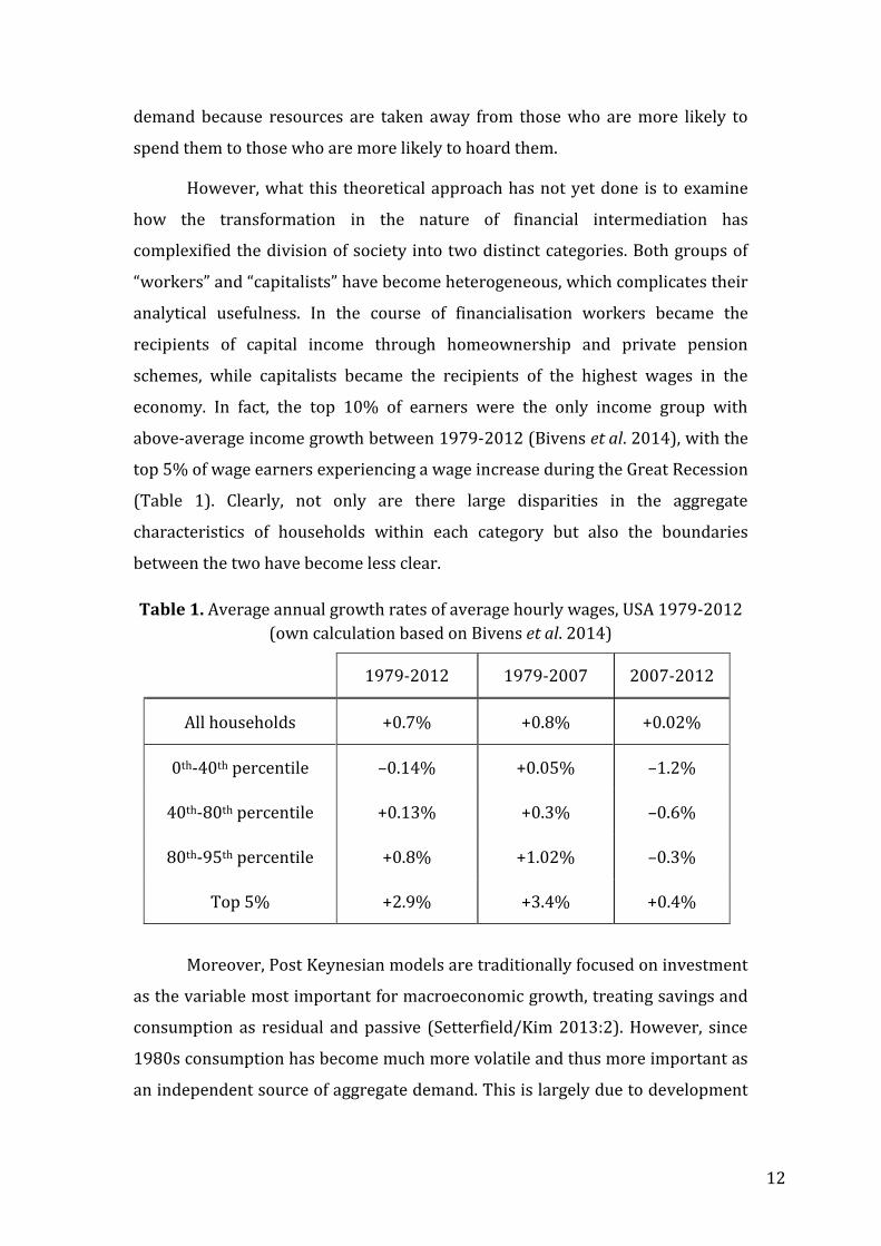
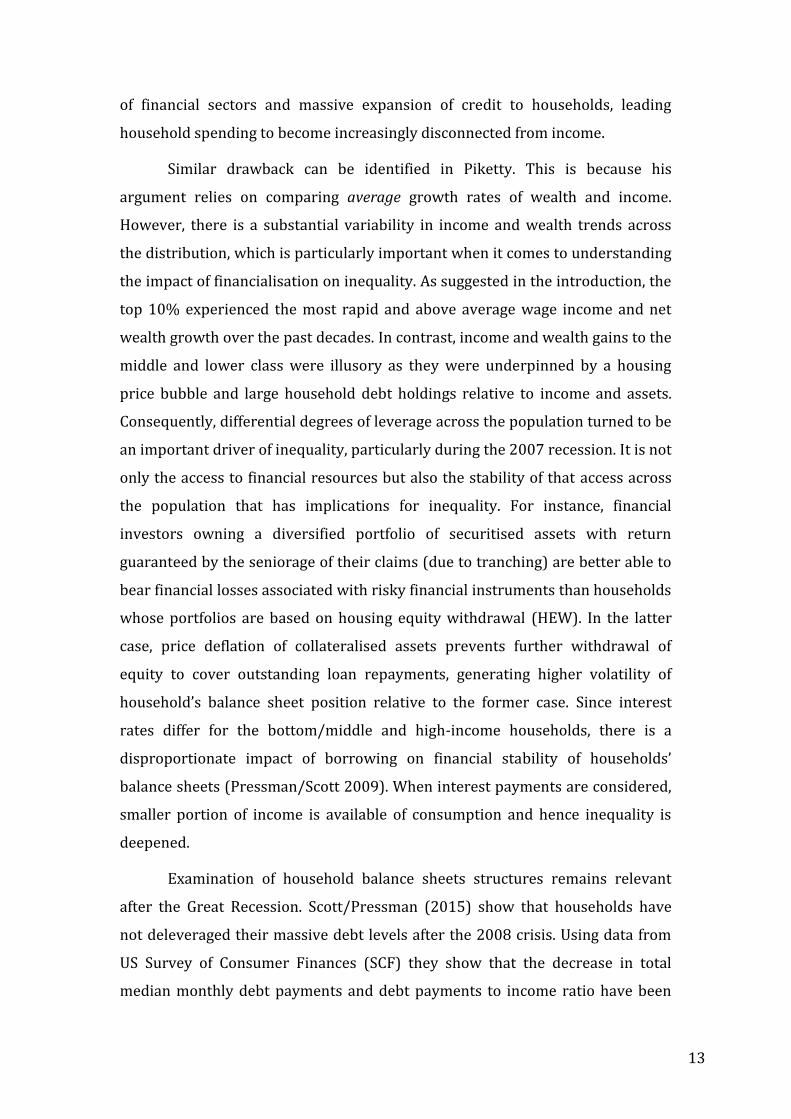
(Table 1). Clearly, not only are there large disparities in the aggregate
characteristics of households within each category but also the boundaries
between the two have become less clear.
Table 1. Average annual growth rates of average hourly wages, USA 1979-2012
(own calculation based on Bivens et al. 2014)
Moreover, Post Keynesian models are traditionally focused on investment
as the variable most important for macroeconomic growth, treating savings and
consumption as residual and passive (Setterfield/Kim 2013:2). However, since
1980s consumption has become much more volatile and thus more important as
an independent source of aggregate demand. This is largely due to development
1979-2012 1979-2007 2007-2012
All households +0.7% +0.8% +0.02%
0th-40th percentile –0.14% +0.05% –1.2%
40th-80th percentile +0.13% +0.3% –0.6%
80th-95th percentile +0.8% +1.02% –0.3%
Top 5% +2.9% +3.4% +0.4%
13
of financial sectors and massive expansion of credit to households, leading
household spending to become increasingly disconnected from income.
Similar drawback can be identified in Piketty. This is because his
argument relies on comparing average growth rates of wealth and income.
However, there is a substantial variability in income and wealth trends across
the distribution, which is particularly important when it comes to understanding
the impact of financialisation on inequality. As suggested in the introduction, the
top 10% experienced the most rapid and above average wage income and net
wealth growth over the past decades. In contrast, income and wealth gains to the
middle and lower class were illusory as they were underpinned by a housing
price bubble and large household debt holdings relative to income and assets.
Consequently, differential degrees of leverage across the population turned to be
an important driver of inequality, particularly during the 2007 recession. It is not
only the access to financial resources but also the stability of that access across
the population that has implications for inequality. For instance, financial
investors owning a diversified portfolio of securitised assets with return
guaranteed by the seniorage of their claims (due to tranching) are better able to
bear financial losses associated with risky financial instruments than households
whose portfolios are based on housing equity withdrawal (HEW). In the latter
case, price deflation of collateralised assets prevents further withdrawal of
equity to cover outstanding loan repayments, generating higher volatility of
household’s balance sheet position relative to the former case. Since interest
rates differ for the bottom/middle and high-income households, there is a
disproportionate impact of borrowing on financial stability of households’
balance sheets (Pressman/Scott 2009). When interest payments are considered,
smaller portion of income is available of consumption and hence inequality is
deepened.
Examination of household balance sheets structures remains relevant
after the Great Recession. Scott/Pressman (2015) show that households have
not deleveraged their massive debt levels after the 2008 crisis. Using data from
US Survey of Consumer Finances (SCF) they show that the decrease in total
median monthly debt payments and debt payments to income ratio have been
14
illusory and reflected low interest rates rather than real reduction in debt. In
fact, mortgage debt levels have not fallen much since the recession. Moreover,
the share of households filing for bankruptcy has been rising since 2010. Because
households have not deleveraged properly after the Great Recession, there have
been no increases in consumption and saving allowing for more equitable
growth of the economy.
Consequently, there is a gap in the existing literature on inequality. On the
one hand, Piketty’s insight on the interplay between wealth and income is not
fully developed on a theoretical level. On the other hand, the Post Keynesian
theoretical literature does not take into sufficiently explore the role of wealth
distribution for overall inequality dynamics. This provides an opportunity to
complement the existing literature with a theoretical model incorporating
wealth into the analysis of inequality. We propose a three-class theoretical
model aiming to explain the observed trends in inequality, accounting for
disparate wage growth, unequal returns to wealth and leverage across the
population and the role played by the middle class.
Definition of the middle class is a complex task as it can be considered
along a variety of dimensions. In monetary terms it is defined, according to the
relative size of income, as the middle 60% of the population, with incomes
ranging from 75% to 125% of median income as the standard, although some
studies have extended the upper limit to as much as 300% of median income
(this is because with 125% as the cut-off a disproportionately large portion of
the population in certain countries falls into the upper class category, cf.
Pressman 2007). Atkinson/Brandolini (2011) develop a wealth criterion to
qualify the income definition of the middle class. Based on various studies, the
rich can be classified as having net wealth at least 30 times larger than mean
income. As for the lower cut-off point, members of the middle class should have
enough real and financial assets to be clear from the risk of falling into poverty
for a certain period of time, e.g. 6 months, if income suddenly falls.
Atkinson/Brandolini argue that asset-poor individuals may need to be excluded
from the middle class even if their income exceeds the poverty threshold.
Furthermore, classification of the middle class depends on social criteria such as
15
class consciousness, social status, lifestyle and type of employment, which
influences individual’s economic security and prospects.
In the Post Keynesian literature, Palley (2015) constitutes one of the first
attempts at formalising the middle class. He models a Goodwinian three-class
economy, with household sector divided into upper, middle and working class
according to the type of employment. Class membership is defined through
capital ownership terms. Upper class is identified with the richest 1% of the
population, corresponding to the top managers. The middle class consisting of
middle managers is defined as the next 19% and hence is much smaller than
traditionally envisaged in the literature and does not contain the median
household. The working class is the bottom 80% and consists of non-supervisory
production workers. Palley’s model introduces a complex class struggle, where
the middle managerial class has conflicts with both the upper and the working
class. Managerial pay is seen as a deduction from surplus in line with Kalecki
(1971), as top managers receive a share of firms’ profit. In contrast, middle
managers’ pay is treated, as is the non-managerial wage, as part of the wage bill
and hence the cost of production based on which the mark-up prices are
determined. Moreover, while non-managerial workers are paid hourly, middle
managers receive a salary. The workers’ share of the wage bill is dependent on
exogenously determined labour bargaining power as well as employment rate
and working hours. Middle and top managers save part of their income, while
workers are traditionally assumed to consume all their wages. Hence, since
middle managers own part of the capital stock, transfer of income towards non-
managerial workers increases consumption. Similarly, because middle managers
have larger propensity to consume than top managers, increase in middle
managerial income boosts consumption. In this setting, class conflict is
complexified as the middle class benefits from higher profit share (which aligns
their interests with those of top managers) as well as from a higher wage share
(creating a common interest with the working class). Simultaneously, it is in
conflict with both the top managerial and working class over the share of profits
and the wage bill respectively. The political alliance of the middle class will
ultimately depend on which source of income – wages or capital – is preferred
(Palley 2015:240).
16
While Palley’s model constitutes an important contribution to the
literature, its conclusions concern the functional distribution of income. The
middle class is argued to have contradicting interests and conflicts with the
upper and lower income groups. However, as argued before, the process of
financialisation harmed the middle class’ wealth and incomes, making their fate
more similar to the working class in terms of class and power struggle. Since the
task of our analysis is to incorporate wealth aspects into the analysis of
inequality in the age of financial sector transformation and since distribution is
interpreted through household balance sheets rather than wage/profit shares, a
new conceptualisation of the middle class is proposed below.
III. Wealth and inequality in stock-flow consistent models
To maintain dialogue with the existing literature on financialisation and
distribution described above, we adopt the method frequently used among the
Post Keynesians, namely the stock flow consistent modelling (thereby SFCM).
Originating in Copeland (1949) and the works of Tobin and Godley in 1980s, the
framework has recently been formalised by Godley/Lavoie (2007). It is a
macroeconomic tool integrating stocks and flows across real and financial
sectors in the economy in a consistent fashion, relying on the quadruple-entry
system, which necessitates that every inflow has a corresponding outflow in the
system (Caverzasi/Godin 2013).
A number of recent contributions in the SFCM literature take into account
some aspects of household wealth into the analyses of growth and
macroeconomic stability (Zezza 2008; Caversazi/Godin 2013; Setterfield/Kim
2013; Nikolaidi 2015; Sawyer/Passarella Veronese 2015;
Dafermos/Papatheodorou 2015). Most commonly, it is by allowing for
borrowing by workers, whose debt becomes financial assets of the rentiers via
banks. Wealth of rentiers is usually divided into equities and deposits and
allocation between these two components depends on the relative rates of
return. We argue, however, that current analyses do not adequately capture the
impact of financialisation on balance sheet structures of different households
and hence inequality. The models do not consider the importance of the middle
17
class in this context as the standard two-class division of households into
workers and capitalists prevails.
With the exception of Dafermos/Papatheodorou (2015), most of the
SFCMs reviewed above do not explain income distribution endogenously. This is
because they are ultimately concerned with macroeconomic growth and
stability. Consequently, analysis of household balance sheets based on the
division of society in two classes of workers and capitalists encounters the same
difficulties as described in the previous section, namely that they do not
sufficiently account for the heterogeneity of wealth among different households.
Apart from Sawyer/Passarella Veronese (2015) borrowing is restricted to
workers, while in most high-income countries it is the rich who are indebted the
most both in terms of value and participation (Survey of Consumer Finances).
Furthermore, few of the studies reviewed above take into account changes
within the financial sector brought about by financialisation – Nikolaidi (2015)
and Sawyer/Passarella Veronese (2015) constitute one of the few analyses
incorporating a sophisticated financial sector. Consequently, the proposed model
attempts to fill the emergent gap in the literature, providing an analysis of
endogenous inequality determination in an economy with a complex financial
sector. Emphasis is put on balance sheet structures within the household sector
and, in particular, different levels of leverage across the population.
IV. Model specification
The aim of the model presented in this paper is to account for household wealth
dynamics in explaining inequality in a financialised economy, using the
benchmark framework developed by Dafermos/Papatheodorou (2015). The US
economy is taken as an example. The methodology of SFCM yields itself to
consideration of the reinforcing dynamics between stocks of wealth and flows of
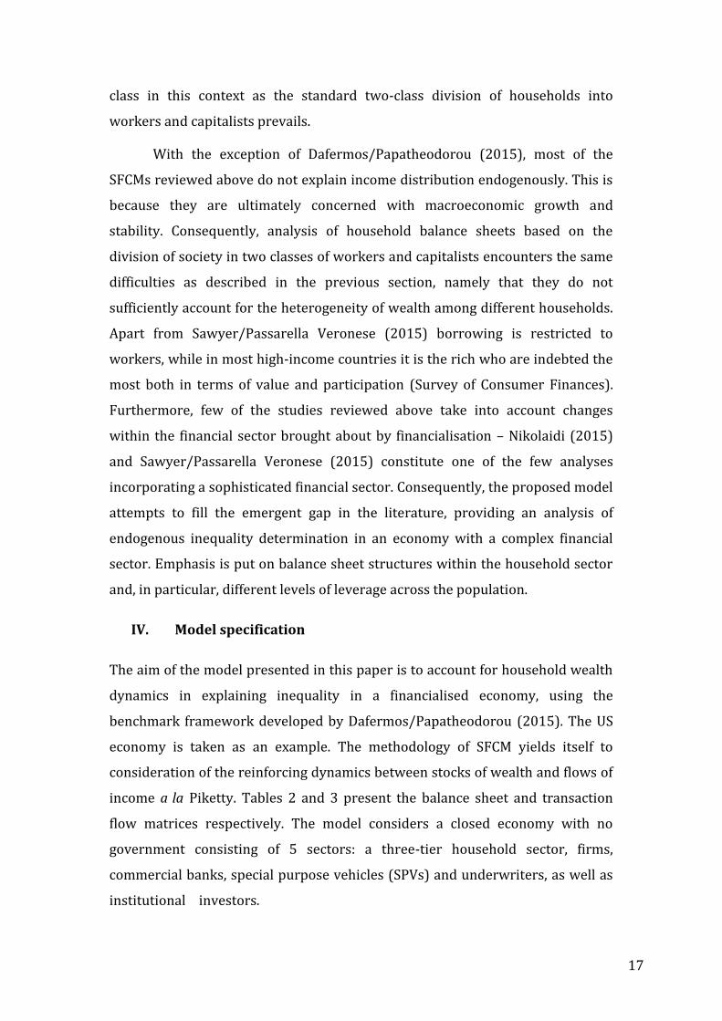
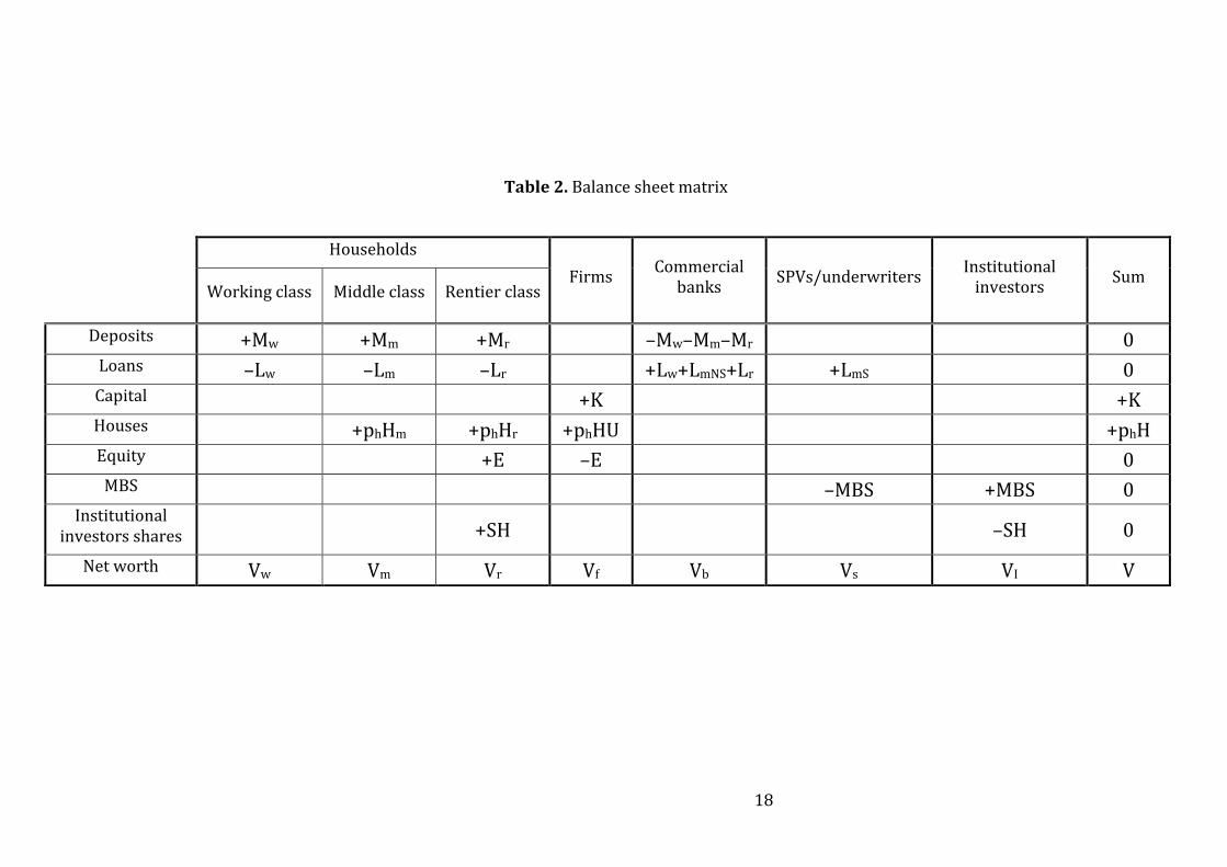
income a la Piketty. Tables 2 and 3 present the balance sheet and transaction
flow matrices respectively. The model considers a closed economy with no
government consisting of 5 sectors: a three-tier household sector, firms,
commercial banks, special purpose vehicles (SPVs) and underwriters, as well as
institutional investors. m
18
Table 2. Balance sheet matrix
Households
Firms Commercial
banks SPVs/underwriters
Institutional investors
Sum Working class Middle class Rentier class
Deposits +Mw +Mm +Mr –Mw–Mm–Mr 0 Loans –Lw –Lm –Lr +Lw+LmNS+Lr +LmS 0 Capital +K +K Houses +phHm +phHr +phHU +phH Equity +E –E 0 MBS –MBS +MBS 0
Institutional investors shares +SH –SH 0
Net worth Vw Vm Vr Vf Vb Vs VI V
19
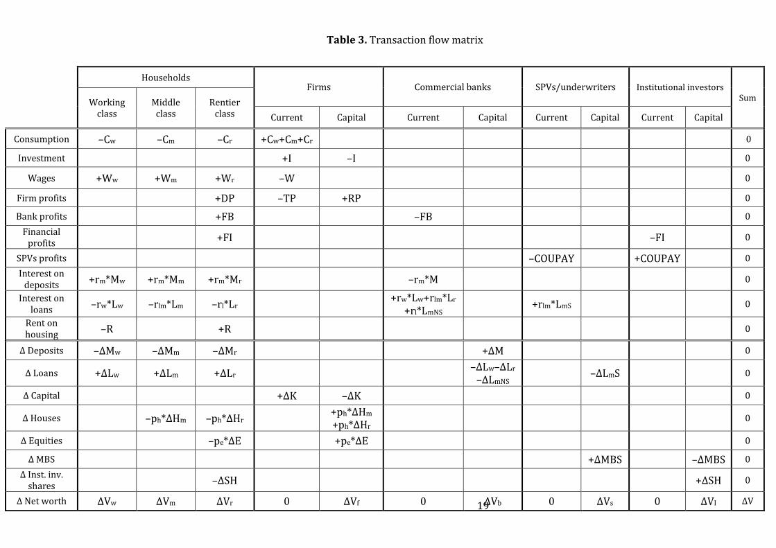
Table 3. Transaction flow matrix
Households Firms Commercial banks SPVs/underwriters Institutional investors
Sum Working class
Middle class
Rentier class Current Capital Current Capital Current Capital Current Capital
Consumption –Cw –Cm –Cr +Cw+Cm+Cr 0
Investment +I –I 0
Wages +Ww +Wm +Wr –W 0
Firm profits +DP –TP +RP 0
Bank profits +FB –FB 0
Financial profits
+FI –FI 0
SPVs profits –COUPAY +COUPAY 0
Interest on deposits
+rm*Mw +rm*Mm +rm*Mr –rm*M 0
Interest on loans
–rw*Lw –rlm*Lm –rl*Lr +rw*Lw+rlm*Lr
+rl*LmNS +rlm*LmS 0
Rent on housing
–R +R 0
Δ Deposits –ΔMw –ΔMm –ΔMr +ΔM 0
Δ Loans +ΔLw +ΔLm +ΔLr –ΔLw–ΔLr
–ΔLmNS –ΔLmS 0
Δ Capital +ΔK –ΔK 0
Δ Houses –ph*ΔHm –ph*ΔHr +ph*ΔHm +ph*ΔHr
0
Δ Equities –pe*ΔE +pe*ΔE 0
Δ MBS +ΔMBS –ΔMBS 0
Δ Inst. inv. shares
–ΔSH +ΔSH 0
Δ Net worth ΔVw ΔVm ΔVr 0 ΔVf 0 ΔVb 0 ΔVs 0 ΔVI ΔV
20
The household sector
In contrast to the existing Post Keynesian approaches to distribution, social
groups in our analysis are defined not by the type of employment or ownership
of the means of production but by their balance sheet characteristics. As argued
previously, this is a more suitable method to understanding inequality in the age
of financial sector transformation and massive indebtedness of the society.
Moreover, it links with the theory developed by Piketty, which highlights the
importance of wealth in contributing to overall inequality.
The working class
Classification of the working class in the present model is conceptually the
closest to the “workers” category encountered in the literature. The working
class includes non-supervisory production/“blue collar” workers. In line with the
Kaleckian approach, this group has the highest propensity to consume. Critically,
they are the most leveraged group. It is identified with the bottom 40% of US
population, which experience net wealth losses over the past three decades (see
fig.5 above).
One of the phenomena associated with financial sector transformation
has been the massive extension of credit to those previously excluded from
access to it based on their low incomes and low or non-existent wealth. As was
argued before, this credit expansion wasn’t accidental as household loans,
primarily mortgages and consumer credit, constituted the basis for asset-backed
securities. Consequently, there were strong incentives in the financial sector to
generate as many household loans as possible to satisfy the growing demands of
financial investors for securitised instruments. For these reasons, analysis of the
household sector in the model accounting for financial sector transformation
calls for consideration of credit among the lowest income groups. In the present
model, the working class households are seen as subprime borrowers. We
assume that they do not carry enough wealth and income that would allow them
to take out mortgages and hence that all working class households rent houses.
Consequently, it is assumed that credit to the working class households consists
of unsecured short-term consumer credit and payday loans. This has been
particularly relevant in recent years as unsecured debt and payday borrowing
21
have been on the rise after the crisis (cf. The Pew Charitable Trust 2012; PWC
2015).
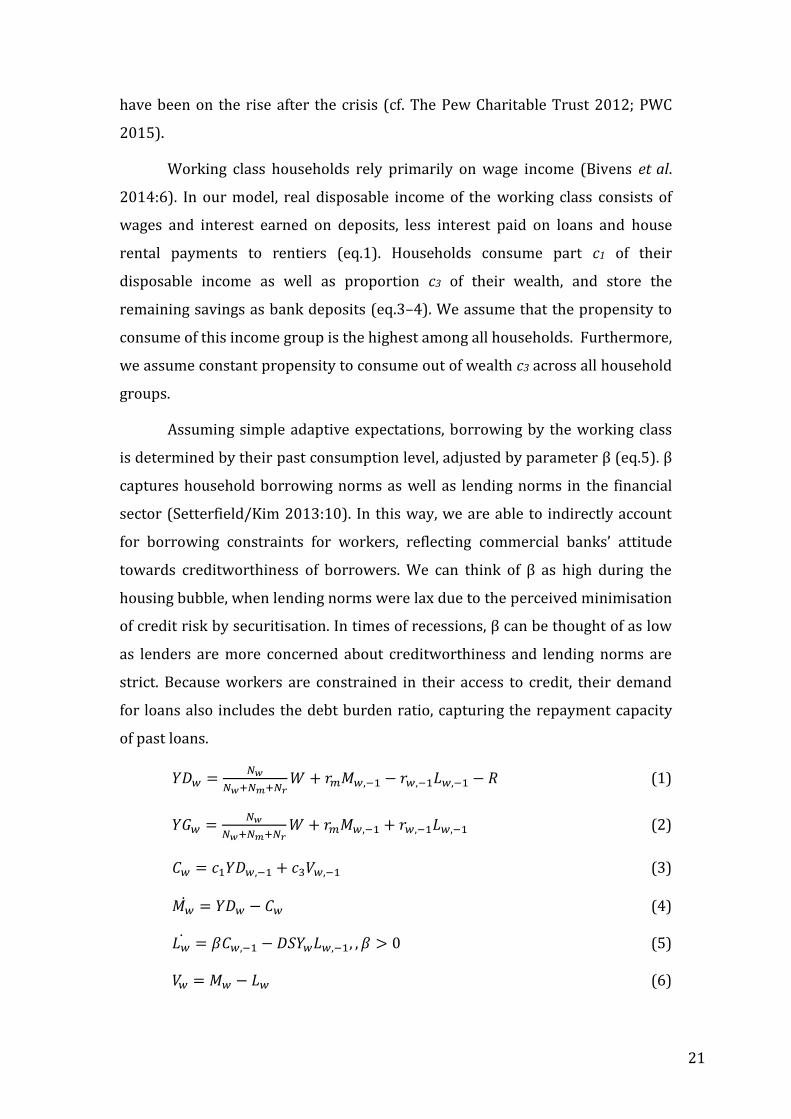
Working class households rely primarily on wage income (Bivens et al.
2014:6). In our model, real disposable income of the working class consists of
wages and interest earned on deposits, less interest paid on loans and house
rental payments to rentiers (eq.1). Households consume part c1 of their
disposable income as well as proportion c3 of their wealth, and store the
remaining savings as bank deposits (eq.3–4). We assume that the propensity to
consume of this income group is the highest among all households. Furthermore,
we assume constant propensity to consume out of wealth c3 across all household
groups.
Assuming simple adaptive expectations, borrowing by the working class
is determined by their past consumption level, adjusted by parameter β (eq.5). β
captures household borrowing norms as well as lending norms in the financial
sector (Setterfield/Kim 2013:10). In this way, we are able to indirectly account
for borrowing constraints for workers, reflecting commercial banks’ attitude
towards creditworthiness of borrowers. We can think of β as high during the
housing bubble, when lending norms were lax due to the perceived minimisation
of credit risk by securitisation. In times of recessions, β can be thought of as low
as lenders are more concerned about creditworthiness and lending norms are
strict. Because workers are constrained in their access to credit, their demand
for loans also includes the debt burden ratio, capturing the repayment capacity
of past loans.
𝑌𝐷𝑤 =𝑁𝑤
𝑁𝑤+𝑁𝑚+𝑁𝑟𝑊 + 𝑟𝑚𝑀𝑤,−1 − 𝑟𝑤,−1𝐿𝑤,−1 − 𝑅 (1)
𝑌𝐺𝑤 =𝑁𝑤
𝑁𝑤+𝑁𝑚+𝑁𝑟𝑊 + 𝑟𝑚𝑀𝑤,−1 + 𝑟𝑤,−1𝐿𝑤,−1 (2)
𝐶𝑤 = 𝑐1𝑌𝐷𝑤,−1 + 𝑐3𝑉𝑤,−1 (3)
𝑀�̇� = 𝑌𝐷𝑤 − 𝐶𝑤 (4)
𝐿�̇� = 𝛽𝐶𝑤,−1 − 𝐷𝑆𝑌𝑤𝐿𝑤,−1, , 𝛽 > 0 (5)
𝑉𝑤 = 𝑀𝑤 − 𝐿𝑤 (6)
22
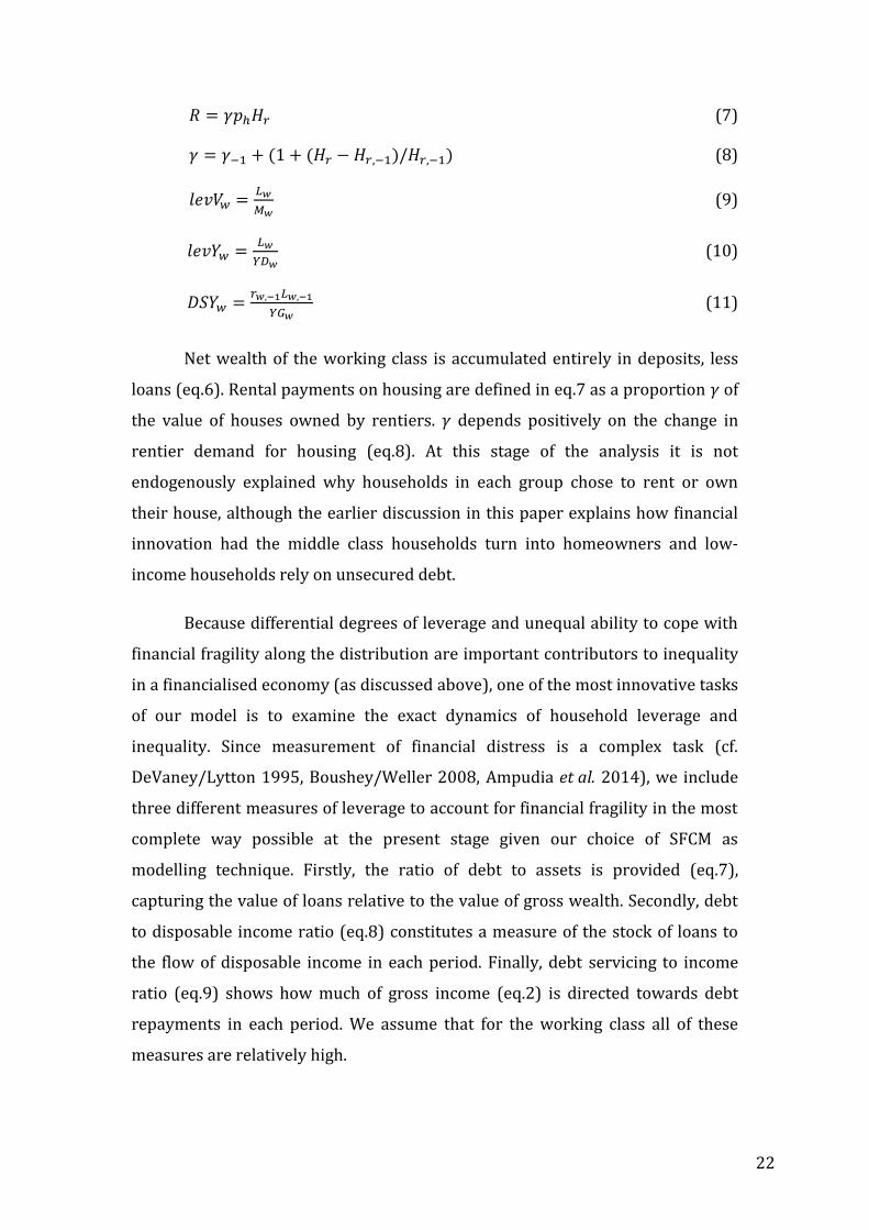
𝑅 = 𝛾𝑝ℎ𝐻𝑟 (7)
𝛾 = 𝛾−1 + (1 + (𝐻𝑟 − 𝐻𝑟,−1)/𝐻𝑟,−1) (8)
𝑙𝑒𝑣𝑉𝑤 =𝐿𝑤
𝑀𝑤 (9)
𝑙𝑒𝑣𝑌𝑤 =𝐿𝑤
𝑌𝐷𝑤 (10)
𝐷𝑆𝑌𝑤 =𝑟𝑤,−1𝐿𝑤,−1
𝑌𝐺𝑤 (11)
Net wealth of the working class is accumulated entirely in deposits, less
loans (eq.6). Rental payments on housing are defined in eq.7 as a proportion 𝛾 of
the value of houses owned by rentiers. 𝛾 depends positively on the change in
rentier demand for housing (eq.8). At this stage of the analysis it is not
endogenously explained why households in each group chose to rent or own
their house, although the earlier discussion in this paper explains how financial
innovation had the middle class households turn into homeowners and low-
income households rely on unsecured debt.
Because differential degrees of leverage and unequal ability to cope with
financial fragility along the distribution are important contributors to inequality
in a financialised economy (as discussed above), one of the most innovative tasks
of our model is to examine the exact dynamics of household leverage and
inequality. Since measurement of financial distress is a complex task (cf.
DeVaney/Lytton 1995, Boushey/Weller 2008, Ampudia et al. 2014), we include
three different measures of leverage to account for financial fragility in the most
complete way possible at the present stage given our choice of SFCM as
modelling technique. Firstly, the ratio of debt to assets is provided (eq.7),
capturing the value of loans relative to the value of gross wealth. Secondly, debt
to disposable income ratio (eq.8) constitutes a measure of the stock of loans to
the flow of disposable income in each period. Finally, debt servicing to income
ratio (eq.9) shows how much of gross income (eq.2) is directed towards debt
repayments in each period. We assume that for the working class all of these
measures are relatively high.
23
The middle class
As suggested previously, definition of the middle class in our model differs
sharply from Palley’s analysis as it is centred on the stylised facts on balance
sheet composition and income trends found in the income and wealth data for
USA.
Importantly, the middle class is defined as a group whose balance sheets
depend on housing. Their wealth was rising in the 1990s and 2000s due to
increasing house prices, allowing them to refinance their mortgages by taking on
more credit and engage in home equity withdrawal, a strategy which was only
feasible in house price bubble. When the price trends reversed during 2006 and
2007, these households saw their wealth gains largely wipe out. Separation of
this group from the working class is important as the evidence shows that in USA
inequality growth has been the most striking between the middle and upper
parts of the population rather than between the top and the bottom (cf. Wolff
2014). This is because of the differential rates of return on wealth of the upper
and middle income groups as well as stagnant income for the latter. For these
reasons, the middle class is assumed to have high leverage ratios.
Our definition of the middle class encompasses the portion of the
population between the 40th and the 90th percentile and thus includes the
median household. The lower cut-off has been chosen as households below the
40th percentile saw negative wage and net worth growth between 1989-2013
(see table 1 and fig.5). In contrast, the upper cut-off has been chosen as only
households above the 90th percentile experienced above average income growth
(Bivens et al. 2014).
Because the middle class is assumed to account for 50% of population in
our analysis, issues associated with heterogeneity of this group need to be
acknowledged. Currently, the middle class in our model includes both subprime
mortgage borrowers, whose incomes resemble more the income of the working
class, and the middle-managers in the 80th-90th percentile, whose incomes and
wealth are closer to the rentier households.
24
We argue that heterogeneity issues cannot be avoided in analysing the
household sector. Three class division adopted here is superior to the two-class
conceptualisation of households in the literature because it allows for a more
intricate examination of household balance sheets, leverage and incomes in the
age of financialisation, which altered the traditionally envisaged economic
relationships. There is a possibility of extending the division of households even
further, which has been done by Dafermos/Papatheodorou (2015). Such detailed
division is not necessary in the present model for two reasons. Firstly, it would
introduce a considerable degree of complexity to an already elaborate model of
heterogeneous households and financial institutions. Secondly, in an aggregate
model that SFCM is, it would be difficult to meaningfully break down the social
classes into upper/lower groups and introduce a drastically different picture of
balance sheets than already provided in the three class model. This is because at
the aggregate level the most important distinctions between the different types
of debt and wealth accumulation possibilities are already made.
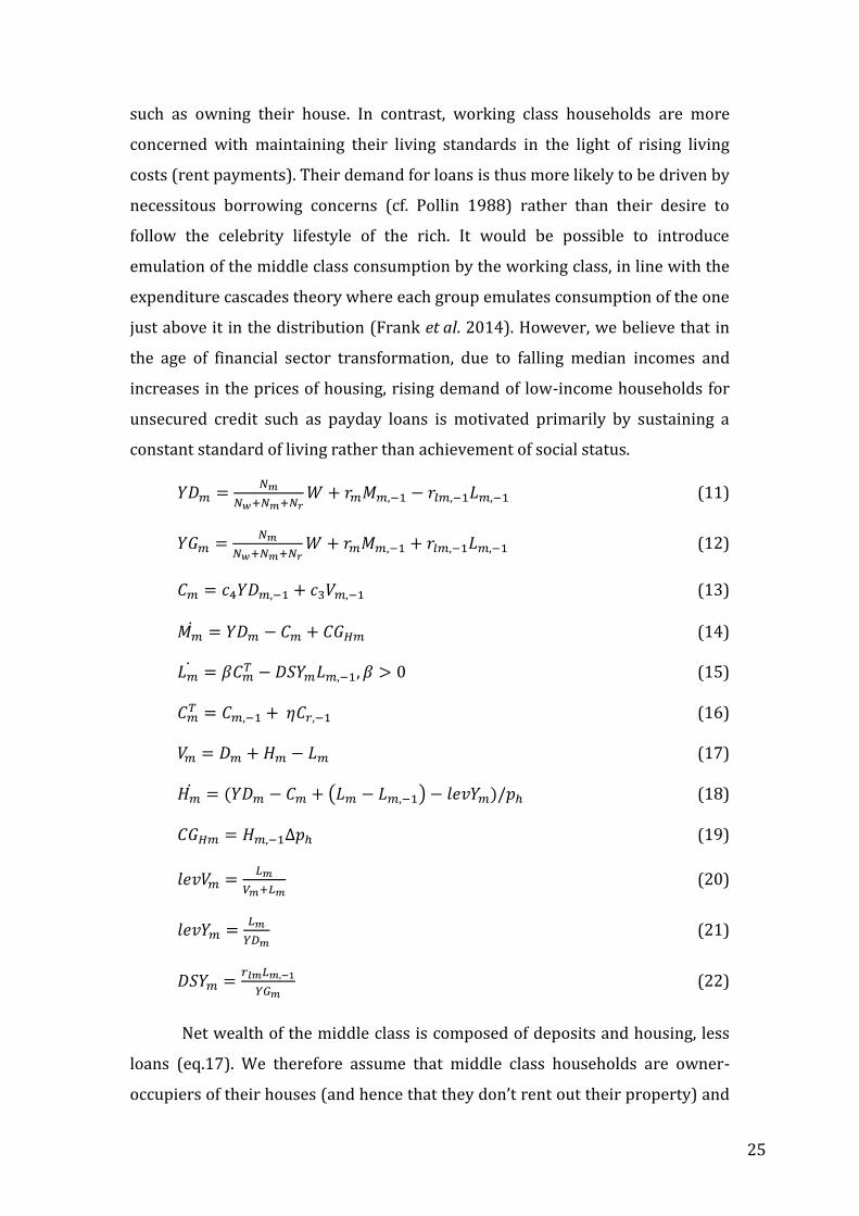
Real disposable income of the middle class consists of wage income and
interest earned on deposits less interest payments on loans (eq.10). A fraction of
disposable income and wealth is consumed (eq.13). Residual income is saved as
deposits, including realised capital gains on housing (eq.14).
Borrowing of the middle class depends on their target consumption and
their debt burden (eq.15). Target consumption incorporates past consumption
(due to simple adaptive expectations) and relative consumption concerns, which
depend on rentier consumption adjusted by an emulation parameter η (eq.16). η
is exogenously defined as the Ravina emulation parameter (Ravina 2007).
Consumption emulation has recently emerged as a potentially important driver
of borrowing (cf. Cynamon/Fazzari 2008, Pressman/Scott 2009), leading to
lower levels of consumption than income inequality (cf. Krueger/Perri 2006).
However, while in existing SFCM studies emulation is applied to low-income
workers (see above and Kapeller/Schuetz 2015; Detzer 2016), we restrict
relative consumption to the middle class. This approach is more reflective of
reality as emulation motives are more likely to be relevant among the more
affluent households belonging to the middle class, who can afford necessities
25
such as owning their house. In contrast, working class households are more
concerned with maintaining their living standards in the light of rising living
costs (rent payments). Their demand for loans is thus more likely to be driven by
necessitous borrowing concerns (cf. Pollin 1988) rather than their desire to
follow the celebrity lifestyle of the rich. It would be possible to introduce
emulation of the middle class consumption by the working class, in line with the
expenditure cascades theory where each group emulates consumption of the one
just above it in the distribution (Frank et al. 2014). However, we believe that in
the age of financial sector transformation, due to falling median incomes and
increases in the prices of housing, rising demand of low-income households for
unsecured credit such as payday loans is motivated primarily by sustaining a
constant standard of living rather than achievement of social status.
𝑌𝐷𝑚 =𝑁𝑚
𝑁𝑤+𝑁𝑚+𝑁𝑟𝑊 + 𝑟𝑚𝑀𝑚,−1 − 𝑟𝑙𝑚,−1𝐿𝑚,−1 (11)
𝑌𝐺𝑚 =𝑁𝑚
𝑁𝑤+𝑁𝑚+𝑁𝑟𝑊 + 𝑟𝑚𝑀𝑚,−1 + 𝑟𝑙𝑚,−1𝐿𝑚,−1 (12)
𝐶𝑚 = 𝑐4𝑌𝐷𝑚,−1 + 𝑐3𝑉𝑚,−1 (13)
𝑀�̇� = 𝑌𝐷𝑚 − 𝐶𝑚 + 𝐶𝐺𝐻𝑚 (14)
𝐿�̇� = 𝛽𝐶𝑚𝑇 − 𝐷𝑆𝑌𝑚𝐿𝑚,−1, 𝛽 > 0 (15)
𝐶𝑚𝑇 = 𝐶𝑚,−1 + 𝜂𝐶𝑟,−1 (16)
𝑉𝑚 = 𝐷𝑚 + 𝐻𝑚 − 𝐿𝑚 (17)
𝐻�̇� = (𝑌𝐷𝑚 − 𝐶𝑚 + (𝐿𝑚 − 𝐿𝑚,−1) − 𝑙𝑒𝑣𝑌𝑚)/𝑝ℎ (18)
𝐶𝐺𝐻𝑚 = 𝐻𝑚,−1∆𝑝ℎ (19)
𝑙𝑒𝑣𝑉𝑚 =𝐿𝑚
𝑉𝑚+𝐿𝑚 (20)
𝑙𝑒𝑣𝑌𝑚 =𝐿𝑚
𝑌𝐷𝑚 (21)
𝐷𝑆𝑌𝑚 =𝑟𝑙𝑚𝐿𝑚,−1
𝑌𝐺𝑚 (22)
Net wealth of the middle class is composed of deposits and housing, less
loans (eq.17). We therefore assume that middle class households are owner-
occupiers of their houses (and hence that they don’t rent out their property) and

26
that loans to the middle class consist exclusively mortgages. Demand for houses
by the middle class depends positively on their income and change in the
provision of mortgages and negatively on their consumption and debt-to-income
ratio, adjusted by the price of housing (eq.18). As in the case of the working class,
different measures of financial fragility for the middle class are presented,
including the debt-to-asset ratio (eq.20), debt-to-income ratio (eq.21) and the
debt-service-to-income ratio (eq.22).
Rentier class
Households in this group are defined as the top 10% of the population. In
contrast to the other household groups, they saw income growth equal or above
the average since 1980s (Bivens et al. 2014). Moreover, their balance sheets are
relying primarily on financial wealth rather than housing or wages, which
differentiates this group from the middle and the working class respectively (see
fig.6).
Existing studies accounting for distributional heterogeneity often adopt
social classification from the times of Marx and treat the rich as pure rentiers,
deriving their income purely from capital ownership. This is also envisaged by
Piketty – as wealth becomes inherited and compounding returns to wealth
exceed income growth overtime, the rich abandon work as they are able to live
off the returns to their wealth. While this was true in the pre-Fordist era and
seems like a plausible scenario for the future in light of the deepening wealth
concentration, it doesn’t describe the realities seen since the post-war period.
Data for USA show that inheritance accounts for a small portion of existing
wealth for the rich (Keister/Lee 2014:20). In turn, much of the income of the top
10% derives not only from large returns to capital but also from extremely high
salaries, particularly for financial sector executives (cf. Kaplan/Rauh 2010). To
account for growing wage inequality we can describe the rentier class in our
model as “working rentiers”. This complements the traditional Post Keynesian
view of the capitalist class as owners of capital earning no wage income.
Importantly, the rentier class engages in work not because of necessity (as is in
the case of the working and the middle class) but because institutional
conditions made employment an alternative “investment strategy” for the rich
27
along the ownership of capital, as they are able to use their financial power to
influence their earnings.
Furthermore, in contrast to the majority of SFCM studies including debt,
we allow for indebtedness of the rich. This is because the analysis of household
survey data reveals that the top decile undertakes sizeable debt and constitutes
the most indebted income group in terms of both participation and the amount
of debt. Consequently, in our model it is assumed that rentiers borrow from
banks to consume and invest in excess of their wage and capital income. Rentier
borrowing depends positively on their wealth, which serves as a collateral. What
is different about indebtedness of the rich is their leverage. In contrast to other
income groups, debt of the top decile constitutes a small portion of their assets.
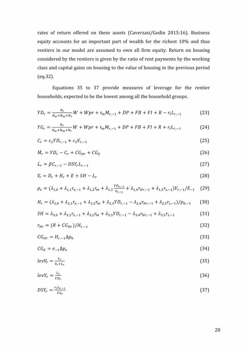
Rentiers’ disposable income consists of wages, interest on deposits,
profits of firms, commercial banks and institutional investors, return on equity,
institutional investors’ shares as well as housing rent payments by the working
class households, less interest paid on loans (eq.23). As other household groups,
rentiers consume a fraction of their income and wealth (eq.25). In line with
Kalecki, rentiers are assumed to have the lowest propensity to consume among
all household groups. Deposits of rentiers consist of residual saving as well as
realised capital gains on housing and equity (eq.26).
Borrowing of rentiers (eq.27) depends on their past consumption and
debt burden ratio and does not include relative consumption concerns. It should
be mentioned, however, that since growth in the national income share of the top
10% is driven by the top 1%, and the growth of the top 1% share is driven by the
top 0.1% (cf. Piketty 2014), relative consumption motives are bound to be
especially strong among the richest 10%, who engage in luxury goods
consumption and aim to attain the highest status and the associated “celebrity
lifestyle”. However, high aggregation of SFCM and the elaborate character of the
current model prevent us from modelling the precise consumption behaviour of
different income groups within the top 10%.
It is assumed that the allocation of rentiers’ wealth between houses,
equities, institutional investors’ shares and deposits (treated as a buffer stock)
(eq.29–31) follows a Tobinesque portfolio principle and depends on the relative
28
rates of return offered on these assets (Caverzasi/Godin 2015:16). Business
equity accounts for an important part of wealth for the richest 10% and thus
rentiers in our model are assumed to own all firm equity. Return on housing
considered by the rentiers is given by the ratio of rent payments by the working
class and capital gains on housing to the value of housing in the previous period
(eq.32).
Equations 35 to 37 provide measures of leverage for the rentier
households, expected to be the lowest among all the household groups.
𝑌𝐷𝑟 =𝑁𝑟
𝑁𝑤+𝑁𝑚+𝑁𝑟𝑊 + 𝑊𝑝𝑟 + 𝑟𝑚𝑀𝑟,−1 + 𝐷𝑃 + 𝐹𝐵 + 𝐹𝐼 + 𝑅 − 𝑟𝑙𝐿𝑟,−1 (23)
𝑌𝐺𝑟 =𝑁𝑟
𝑁𝑤+𝑁𝑚+𝑁𝑟𝑊 + 𝑊𝑝𝑟 + 𝑟𝑚𝑀𝑟,−1 + 𝐷𝑃 + 𝐹𝐵 + 𝐹𝐼 + 𝑅 + 𝑟𝑙𝐿𝑟,−1 (24)
𝐶𝑟 = 𝑐2𝑌𝐷𝑟,−1 + 𝑐3𝑉𝑟,−1 (25)
𝑀𝑟̇ = 𝑌𝐷𝑟 − 𝐶𝑟 + 𝐶𝐺𝐻𝑟 + 𝐶𝐺𝐸 (26)
𝐿�̇� = 𝛽𝐶𝑟,−1 − 𝐷𝑆𝑌𝑟𝐿𝑟,−1 (27)
𝑉𝑟 = 𝐷𝑟 + 𝐻𝑟 + 𝐸 + 𝑆𝐻 − 𝐿𝑟 (28)
𝑝𝑒 = (𝜆1,0 + 𝜆1,1𝑟𝑒,−1 + 𝜆1,2𝑟𝑚 + 𝜆1,3𝑌𝐷𝑟,−1
𝑉𝑟,−1+ 𝜆1,4𝑟𝐻𝑟,−1 + 𝜆1,5𝑟𝑠,−1)𝑉𝑟,−1/𝐸−1 (29)
𝐻𝑟 = (𝜆2,0 + 𝜆2,1𝑟𝑒,−1 + 𝜆2,2𝑟𝑚 + 𝜆2,3𝑌𝐷𝑟,−1 − 𝜆2,4𝑟𝐻𝑟,−1 + 𝜆2,5𝑟𝑠,−1)/𝑝ℎ,−1 (30)
𝑆𝐻 = 𝜆3,0 + 𝜆3,1𝑟𝑒,−1 + 𝜆3,2𝑟𝑚 + 𝜆3,3𝑌𝐷𝑟,−1 − 𝜆3,4𝑟𝐻𝑟,−1 + 𝜆3,5𝑟𝑠,−1 (31)
𝑟𝐻𝑟 = (𝑅 + 𝐶𝐺𝐻𝑟)/𝐻𝑟,−1 (32)
𝐶𝐺𝐻𝑟 = 𝐻𝑟,−1∆𝑝ℎ (33)
𝐶𝐺𝐸 = 𝑒−1∆𝑝𝑒 (34)
𝑙𝑒𝑣𝑉𝑟 =𝐿𝑟
𝑉𝑟+𝐿𝑟 (35)
𝑙𝑒𝑣𝑌𝑟 =𝐿𝑟
𝑌𝐷𝑟 (36)
𝐷𝑆𝑌𝑟 =𝑟𝑙𝐿𝑟,−1
𝑌𝐺𝑟 (37)
29
Firms
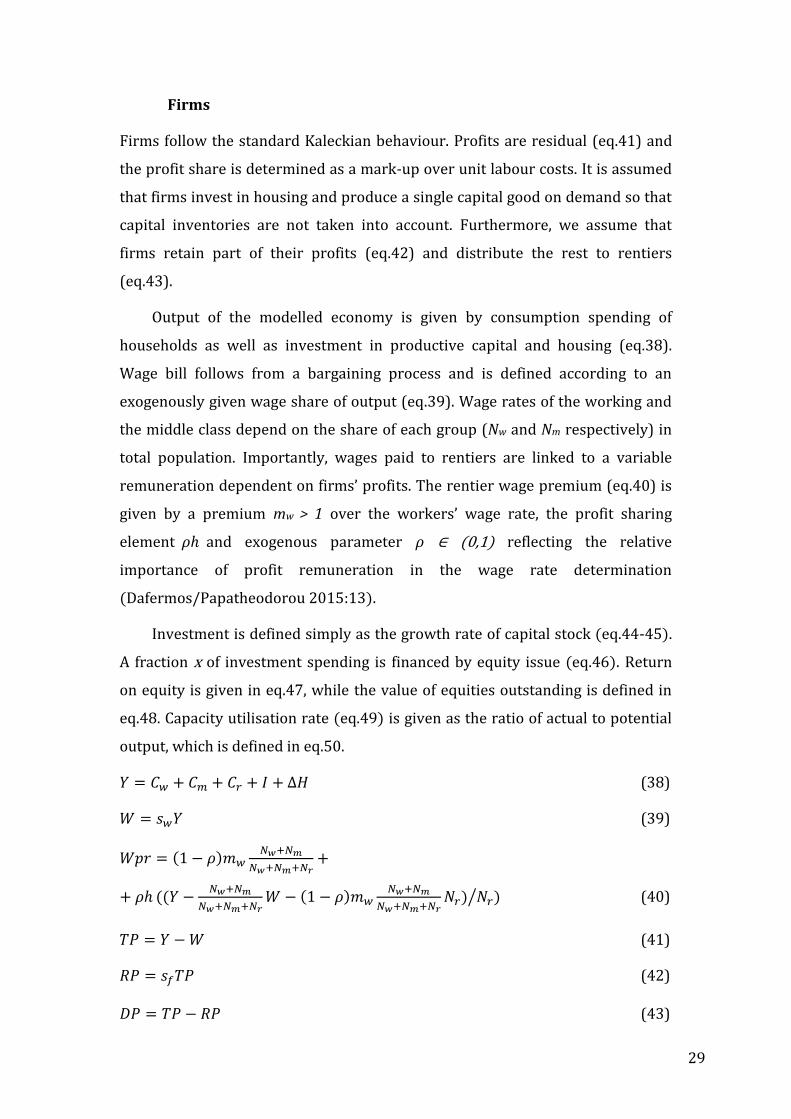
Firms follow the standard Kaleckian behaviour. Profits are residual (eq.41) and
the profit share is determined as a mark-up over unit labour costs. It is assumed
that firms invest in housing and produce a single capital good on demand so that
capital inventories are not taken into account. Furthermore, we assume that
firms retain part of their profits (eq.42) and distribute the rest to rentiers
(eq.43).
Output of the modelled economy is given by consumption spending of
households as well as investment in productive capital and housing (eq.38).
Wage bill follows from a bargaining process and is defined according to an
exogenously given wage share of output (eq.39). Wage rates of the working and
the middle class depend on the share of each group (Nw and Nm respectively) in
total population. Importantly, wages paid to rentiers are linked to a variable
remuneration dependent on firms’ profits. The rentier wage premium (eq.40) is
given by a premium mw > 1 over the workers’ wage rate, the profit sharing
element 𝜌ℎ and exogenous parameter 𝜌 ∈ (0,1) reflecting the relative
importance of profit remuneration in the wage rate determination
(Dafermos/Papatheodorou 2015:13).
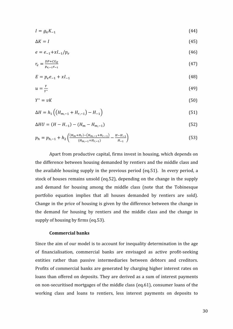
Investment is defined simply as the growth rate of capital stock (eq.44-45).
A fraction x of investment spending is financed by equity issue (eq.46). Return
on equity is given in eq.47, while the value of equities outstanding is defined in
eq.48. Capacity utilisation rate (eq.49) is given as the ratio of actual to potential
output, which is defined in eq.50.
𝑌 = 𝐶𝑤 + 𝐶𝑚 + 𝐶𝑟 + 𝐼 + ∆𝐻 (38)
𝑊 = 𝑠𝑤𝑌 (39)
𝑊𝑝𝑟 = (1 − 𝜌)𝑚𝑤𝑁𝑤+𝑁𝑚
𝑁𝑤+𝑁𝑚+𝑁𝑟+
+ 𝜌ℎ ((𝑌 −𝑁𝑤+𝑁𝑚
𝑁𝑤+𝑁𝑚+𝑁𝑟𝑊 − (1 − 𝜌)𝑚𝑤
𝑁𝑤+𝑁𝑚
𝑁𝑤+𝑁𝑚+𝑁𝑟𝑁𝑟) 𝑁𝑟⁄ ) (40)
𝑇𝑃 = 𝑌 − 𝑊 (41)
𝑅𝑃 = 𝑠𝑓𝑇𝑃 (42)
𝐷𝑃 = 𝑇𝑃 − 𝑅𝑃 (43)
30
𝐼 = 𝑔𝑘𝐾−1 (44)
Δ𝐾 = 𝐼 (45)
𝑒 = 𝑒−1+𝑥𝐼−1/𝑝𝑒 (46)
𝑟𝑒 =𝐷𝑃+𝐶𝐺𝐸
𝑝𝑒,−1𝑒−1 (47)
𝐸 = 𝑝𝑒𝑒−1 + 𝑥𝐼−1 (48)
𝑢 =𝑌
𝑌∗ (49)
𝑌∗ = 𝑣𝐾 (50)
Δ𝐻 = ℎ1 ((𝐻𝑚,−1 + 𝐻𝑟,−1) − 𝐻−1) (51)
Δ𝐻𝑈 = (𝐻 − 𝐻−1) − (𝐻𝑚 − 𝐻𝑚,−1) (52)
𝑝ℎ = 𝑝ℎ,−1 + ℎ2 ((𝐻𝑚+𝐻𝑟)−(𝐻𝑚,−1+𝐻𝑟,−1)
(𝐻𝑚,−1+𝐻𝑟,−1)−
𝐻−𝐻−1
𝐻−1) (53)
Apart from productive capital, firms invest in housing, which depends on
the difference between housing demanded by rentiers and the middle class and
the available housing supply in the previous period (eq.51). In every period, a
stock of houses remains unsold (eq.52), depending on the change in the supply
and demand for housing among the middle class (note that the Tobinesque
portfolio equation implies that all houses demanded by rentiers are sold).
Change in the price of housing is given by the difference between the change in
the demand for housing by rentiers and the middle class and the change in
supply of housing by firms (eq.53).
Commercial banks
Since the aim of our model is to account for inequality determination in the age
of financialisation, commercial banks are envisaged as active profit-seeking
entities rather than passive intermediaries between debtors and creditors.
Profits of commercial banks are generated by charging higher interest rates on
loans than offered on deposits. They are derived as a sum of interest payments
on non-securitised mortgages of the middle class (eq.61), consumer loans of the
working class and loans to rentiers, less interest payments on deposits to
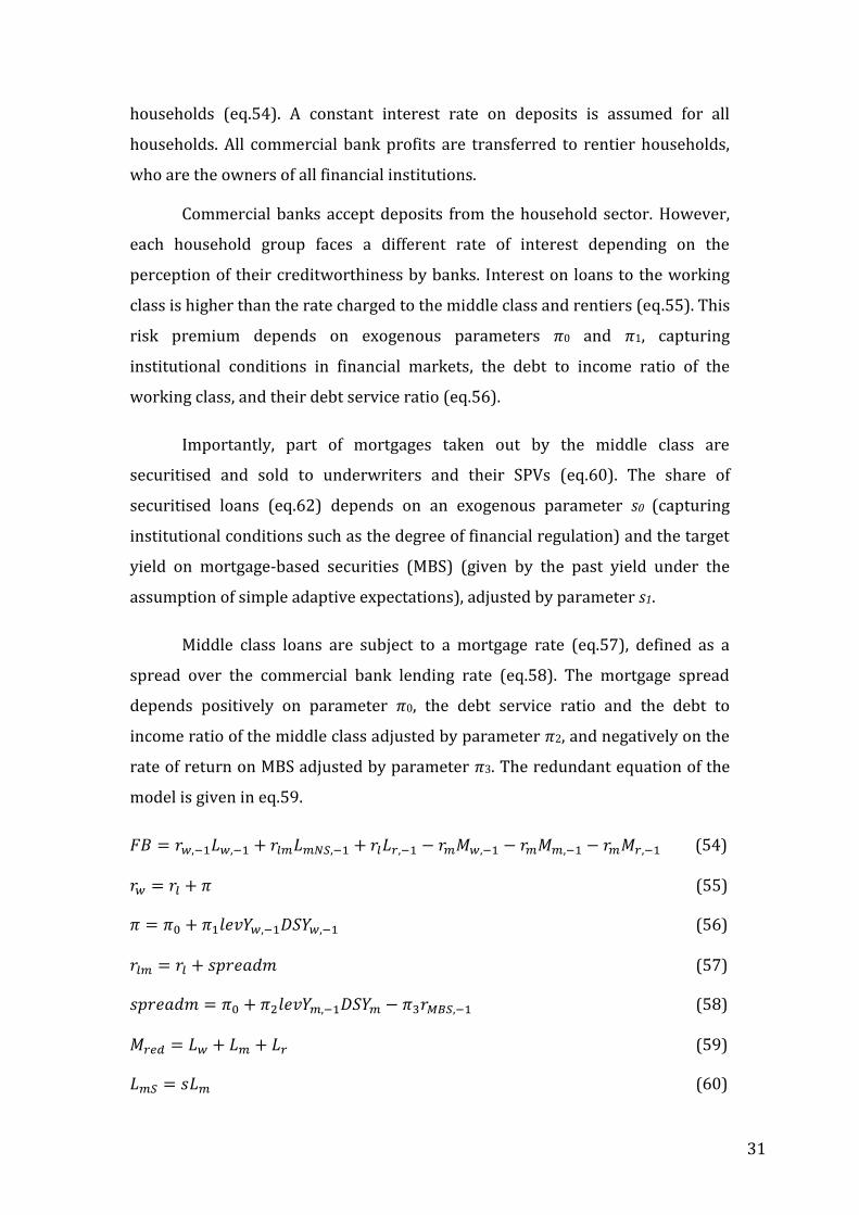
31
households (eq.54). A constant interest rate on deposits is assumed for all
households. All commercial bank profits are transferred to rentier households,
who are the owners of all financial institutions.
Commercial banks accept deposits from the household sector. However,
each household group faces a different rate of interest depending on the
perception of their creditworthiness by banks. Interest on loans to the working
class is higher than the rate charged to the middle class and rentiers (eq.55). This
risk premium depends on exogenous parameters 𝜋0 and 𝜋1, capturing
institutional conditions in financial markets, the debt to income ratio of the
working class, and their debt service ratio (eq.56).
Importantly, part of mortgages taken out by the middle class are
securitised and sold to underwriters and their SPVs (eq.60). The share of
securitised loans (eq.62) depends on an exogenous parameter s0 (capturing
institutional conditions such as the degree of financial regulation) and the target
yield on mortgage-based securities (MBS) (given by the past yield under the
assumption of simple adaptive expectations), adjusted by parameter s1.
Middle class loans are subject to a mortgage rate (eq.57), defined as a
spread over the commercial bank lending rate (eq.58). The mortgage spread
depends positively on parameter 𝜋0, the debt service ratio and the debt to
income ratio of the middle class adjusted by parameter 𝜋2, and negatively on the
rate of return on MBS adjusted by parameter 𝜋3. The redundant equation of the
model is given in eq.59.
𝐹𝐵 = 𝑟𝑤,−1𝐿𝑤,−1 + 𝑟𝑙𝑚𝐿𝑚𝑁𝑆,−1 + 𝑟𝑙𝐿𝑟,−1 − 𝑟𝑚𝑀𝑤,−1 − 𝑟𝑚𝑀𝑚,−1 − 𝑟𝑚𝑀𝑟,−1 (54)
𝑟𝑤 = 𝑟𝑙 + 𝜋 (55)
𝜋 = 𝜋0 + 𝜋1𝑙𝑒𝑣𝑌𝑤,−1𝐷𝑆𝑌𝑤,−1 (56)
𝑟𝑙𝑚 = 𝑟𝑙 + 𝑠𝑝𝑟𝑒𝑎𝑑𝑚 (57)
𝑠𝑝𝑟𝑒𝑎𝑑𝑚 = 𝜋0 + 𝜋2𝑙𝑒𝑣𝑌𝑚,−1𝐷𝑆𝑌𝑚 − 𝜋3𝑟𝑀𝐵𝑆,−1 (58)
𝑀𝑟𝑒𝑑 = 𝐿𝑤 + 𝐿𝑚 + 𝐿𝑟 (59)
𝐿𝑚𝑆 = 𝑠𝐿𝑚 (60)
32
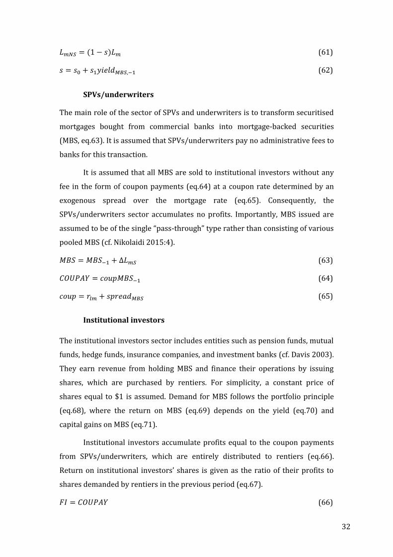
𝐿𝑚𝑁𝑆 = (1 − 𝑠)𝐿𝑚 (61)
𝑠 = 𝑠0 + 𝑠1𝑦𝑖𝑒𝑙𝑑𝑀𝐵𝑆,−1 (62)
SPVs/underwriters
The main role of the sector of SPVs and underwriters is to transform securitised
mortgages bought from commercial banks into mortgage-backed securities
(MBS, eq.63). It is assumed that SPVs/underwriters pay no administrative fees to
banks for this transaction.
It is assumed that all MBS are sold to institutional investors without any
fee in the form of coupon payments (eq.64) at a coupon rate determined by an
exogenous spread over the mortgage rate (eq.65). Consequently, the
SPVs/underwriters sector accumulates no profits. Importantly, MBS issued are
assumed to be of the single “pass-through” type rather than consisting of various
pooled MBS (cf. Nikolaidi 2015:4).
𝑀𝐵𝑆 = 𝑀𝐵𝑆−1 + ∆𝐿𝑚𝑆 (63)
𝐶𝑂𝑈𝑃𝐴𝑌 = 𝑐𝑜𝑢𝑝𝑀𝐵𝑆−1 (64)
𝑐𝑜𝑢𝑝 = 𝑟𝑙𝑚 + 𝑠𝑝𝑟𝑒𝑎𝑑𝑀𝐵𝑆 (65)
Institutional investors
The institutional investors sector includes entities such as pension funds, mutual
funds, hedge funds, insurance companies, and investment banks (cf. Davis 2003).
They earn revenue from holding MBS and finance their operations by issuing
shares, which are purchased by rentiers. For simplicity, a constant price of
shares equal to $1 is assumed. Demand for MBS follows the portfolio principle
(eq.68), where the return on MBS (eq.69) depends on the yield (eq.70) and
capital gains on MBS (eq.71).
Institutional investors accumulate profits equal to the coupon payments
from SPVs/underwriters, which are entirely distributed to rentiers (eq.66).
Return on institutional investors’ shares is given as the ratio of their profits to
shares demanded by rentiers in the previous period (eq.67).
𝐹𝐼 = 𝐶𝑂𝑈𝑃𝐴𝑌 (66)

33
𝑟𝑠 =𝐹𝐼
𝑆𝐻−1 (67)
𝑝𝑀𝐵𝑆 =(𝜃10+𝜃11𝑟𝑀𝐵𝑆,−1)𝑆𝐻−1
𝑀𝐵𝑆 (68)
𝑟𝑀𝐵𝑆 = 𝑦𝑖𝑒𝑙𝑑𝑀𝐵𝑆 +𝐶𝐺𝑀𝐵𝑆
𝑝𝑀𝐵𝑆,−1𝑀𝐵𝑆−1 (69)
𝑦𝑖𝑒𝑙𝑑𝑀𝐵𝑆 =𝐶𝑂𝑈𝑃𝐴𝑌
𝑝𝑀𝐵𝑆,−1𝑀𝐵𝑆−1 (70)
𝐶𝐺𝑀𝐵𝑆 = 𝑀𝐵𝑆−1(𝑝𝑀𝐵𝑆 − 𝑝𝑀𝐵𝑆,−1) (71)
Simulations
The model is calibrated to the US economy (see Appendix). The main objective of
the simulation exercise is to examine the impact of the proposed model on
inequality patters. Specifically, we analyse how changes in household balance
sheet composition and leverage affect quantitative measures of income
inequality such as the Gini index (eq.72), the Atkinson index (with inequality
aversion parameter 𝜀=2 in eq.73) and the squared coefficient of variation
(eq.74). While the Gini and Atkinson indices range between 0 and 1, squared
coefficient of variation ranges from 0 to infinity. In all indices, higher value
indicates higher inequality level. This follows the benchmark exercise outlined in
Dafermos/Papatheodorou (2015) where the choice of these three inequality
measures is motivated by their different sensitivity to inequality in different
moments of the distribution (the middle, the bottom and the top of the
distribution respectively).
In addition, we calculate the Theil T index to capture wealth inequality
(eq.78). This is because the other measures of income inequality incorporated in
our model cannot be readily adapted to the distribution of wealth due to possible
negative net worth values (cf. Cowell 2009:72). Theil T index is a generalised
entropy measure of inequality, ranging between 0 and infinity, higher value
corresponding to a higher inequality level (World Bank 2005). To compare the
distributions of income and wealth in our model, we also compute the Theil T
index for income (eq.77).
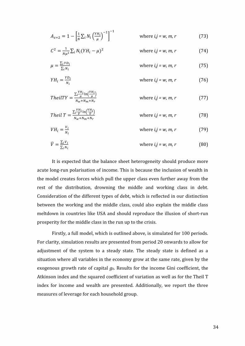
𝐺𝐼𝑁𝐼 =1
2𝑁2𝜇∑ |𝑌𝐻𝑖 − 𝑌𝐻𝑗|𝑁𝑖𝑁𝑗𝑖,𝑗 where i,j = w, m, r (72)
34
𝐴𝜀=2 = 1 − [1
𝑁∑ 𝑁𝑖 (
𝑌𝐻𝑖
𝜇)
−1
𝑖 ]−1
where i,j = w, m, r (73)
𝐶2 =1
𝑁𝜇2∑ 𝑁𝑖(𝑌𝐻𝑖 − 𝜇)2
𝑖 where i,j = w, m, r (74)
𝜇 =∑ 𝑌𝐷𝑖𝑖
∑ 𝑁𝑖𝑖 where i,j = w, m, r (75)
𝑌𝐻𝑖 =𝑌𝐷𝑖
𝑁𝑖 where i,j = w, m, r (76)
𝑇ℎ𝑒𝑖𝑙𝑇𝑌 =∑
𝑌𝐻𝑖𝜇
ln(𝑌𝐻𝑖
𝜇)𝑖
𝑁𝑤+𝑁𝑚+𝑁𝑟 where i,j = w, m, r (77)
𝑇ℎ𝑒𝑖𝑙 𝑇 =∑
𝑉𝐻𝑖�̅�
ln(𝑉𝐻𝑖
�̅�)𝑖
𝑁𝑤+𝑁𝑚+𝑁𝑟 where i,j = w, m, r (78)
𝑉𝐻𝑖 =𝑉𝑖
𝑁𝑖 where i,j = w, m, r (79)
�̅� =∑ 𝑉𝑖𝑖
∑ 𝑁𝑖𝑖 where i,j = w, m, r (80)
It is expected that the balance sheet heterogeneity should produce more
acute long-run polarisation of income. This is because the inclusion of wealth in
the model creates forces which pull the upper class even further away from the
rest of the distribution, drowning the middle and working class in debt.
Consideration of the different types of debt, which is reflected in our distinction
between the working and the middle class, could also explain the middle class
meltdown in countries like USA and should reproduce the illusion of short-run
prosperity for the middle class in the run up to the crisis.
Firstly, a full model, which is outlined above, is simulated for 100 periods.
For clarity, simulation results are presented from period 20 onwards to allow for
adjustment of the system to a steady state. The steady state is defined as a
situation where all variables in the economy grow at the same rate, given by the
exogenous growth rate of capital gk. Results for the income Gini coefficient, the
Atkinson index and the squared coefficient of variation as well as for the Theil T
index for income and wealth are presented. Additionally, we report the three
measures of leverage for each household group.
35
Secondly, we compare the above results of the full model with reduced
form specification without the novel features introduced in our model, namely
rentier wage, rentier debt and securitisation.
V. Results
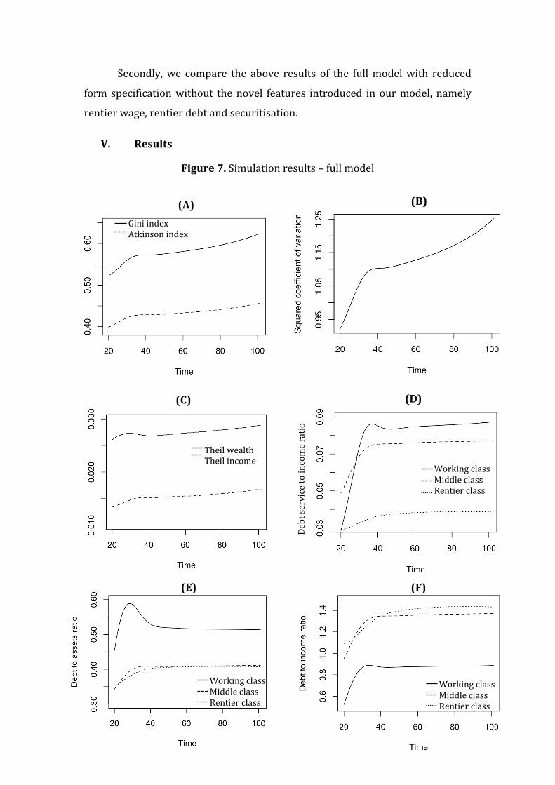
Figure 7. Simulation results – full model
Gini index Atkinson index
Working class Middle class Rentier class
Working class Middle class Rentier class
Working class Middle class Rentier class
Deb
t se
rvic
e to
inco
me
rati
o
(A) (B)
(C) (D)
(E) (F)
Theil wealth Theil income
36
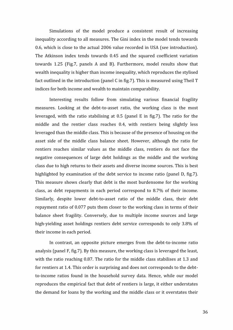
Simulations of the model produce a consistent result of increasing
inequality according to all measures. The Gini index in the model tends towards
0.6, which is close to the actual 2006 value recorded in USA (see introduction).
The Atkinson index tends towards 0.45 and the squared coefficient variation
towards 1.25 (Fig.7, panels A and B). Furthermore, model results show that
wealth inequality is higher than income inequality, which reproduces the stylised
fact outlined in the introduction (panel C in fig.7). This is measured using Theil T
indices for both income and wealth to maintain comparability.
Interesting results follow from simulating various financial fragility
measures. Looking at the debt-to-asset ratio, the working class is the most
leveraged, with the ratio stabilising at 0.5 (panel E in fig.7). The ratio for the
middle and the rentier class reaches 0.4, with rentiers being slightly less
leveraged than the middle class. This is because of the presence of housing on the
asset side of the middle class balance sheet. However, although the ratio for
rentiers reaches similar values as the middle class, rentiers do not face the
negative consequences of large debt holdings as the middle and the working
class due to high returns to their assets and diverse income sources. This is best
highlighted by examination of the debt service to income ratio (panel D, fig.7).
This measure shows clearly that debt is the most burdensome for the working
class, as debt repayments in each period correspond to 8.7% of their income.
Similarly, despite lower debt-to-asset ratio of the middle class, their debt
repayment ratio of 0.077 puts them closer to the working class in terms of their
balance sheet fragility. Conversely, due to multiple income sources and large
high-yielding asset holdings rentiers debt service corresponds to only 3.8% of
their income in each period.
In contrast, an opposite picture emerges from the debt-to-income ratio
analysis (panel F, fig.7). By this measure, the working class is leveraged the least,
with the ratio reaching 0.87. The ratio for the middle class stabilises at 1.3 and
for rentiers at 1.4. This order is surprising and does not corresponds to the debt-
to-income ratios found in the household survey data. Hence, while our model
reproduces the empirical fact that debt of rentiers is large, it either understates
the demand for loans by the working and the middle class or it overstates their
37
income. This may be either because the part of the wage share accruing to the
working and the middle class is overstated in our model compared to the real
world or because the impact of securitisation on household indebtedness does
not generate enough supply and demand for debt among the lower and middle
income groups. Both of these explanations are related to the aggregate nature of
the SFCM method and the inability to decompose the imposed aggregated
structures. Consequently, in the context of our model it is important to examine
household financial fragility holistically, as each of the commonly used measures
provides different information on households’ capacity to handle financial
distress.
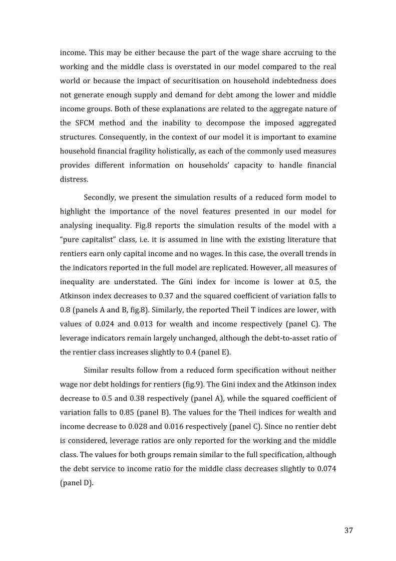
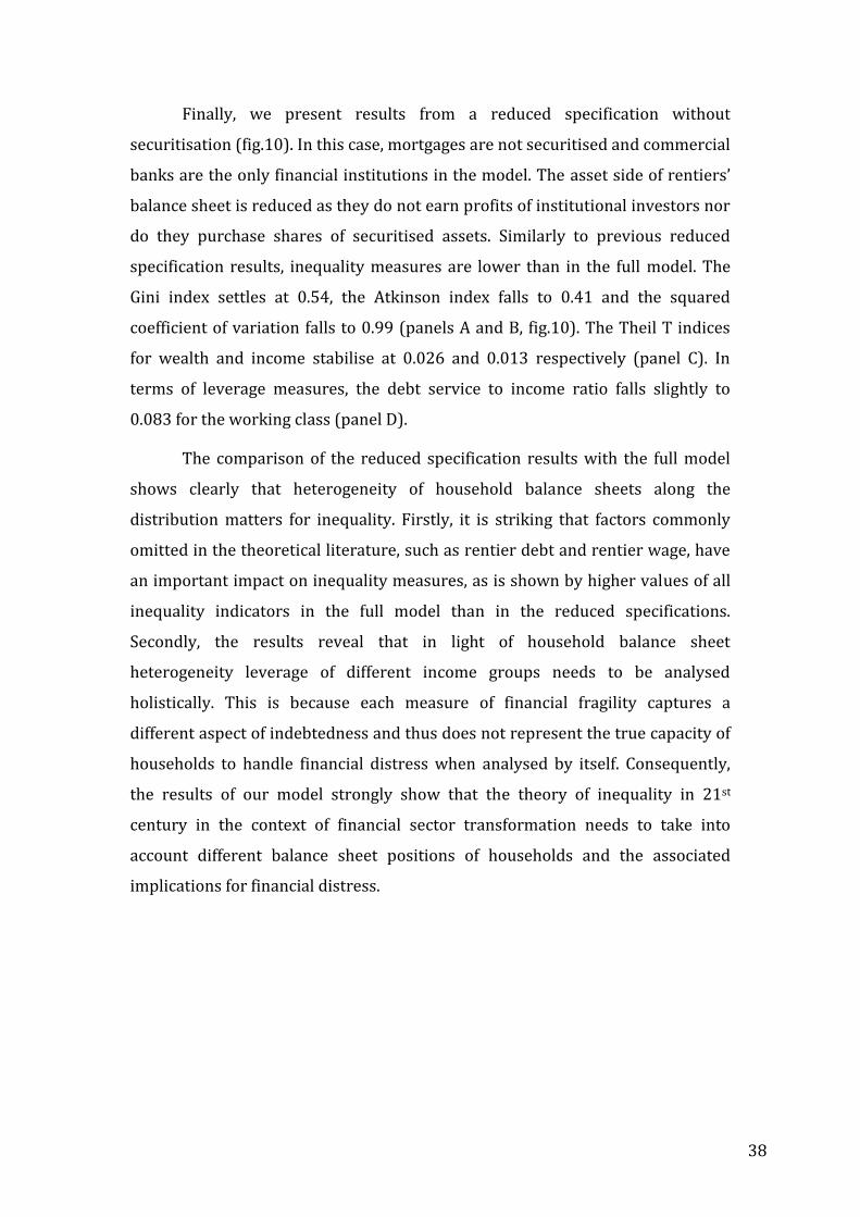
Secondly, we present the simulation results of a reduced form model to
highlight the importance of the novel features presented in our model for
analysing inequality. Fig.8 reports the simulation results of the model with a
“pure capitalist” class, i.e. it is assumed in line with the existing literature that
rentiers earn only capital income and no wages. In this case, the overall trends in
the indicators reported in the full model are replicated. However, all measures of
inequality are understated. The Gini index for income is lower at 0.5, the
Atkinson index decreases to 0.37 and the squared coefficient of variation falls to
0.8 (panels A and B, fig.8). Similarly, the reported Theil T indices are lower, with
values of 0.024 and 0.013 for wealth and income respectively (panel C). The
leverage indicators remain largely unchanged, although the debt-to-asset ratio of
the rentier class increases slightly to 0.4 (panel E).
Similar results follow from a reduced form specification without neither
wage nor debt holdings for rentiers (fig.9). The Gini index and the Atkinson index
decrease to 0.5 and 0.38 respectively (panel A), while the squared coefficient of
variation falls to 0.85 (panel B). The values for the Theil indices for wealth and
income decrease to 0.028 and 0.016 respectively (panel C). Since no rentier debt
is considered, leverage ratios are only reported for the working and the middle
class. The values for both groups remain similar to the full specification, although
the debt service to income ratio for the middle class decreases slightly to 0.074
(panel D).
38
Finally, we present results from a reduced specification without
securitisation (fig.10). In this case, mortgages are not securitised and commercial
banks are the only financial institutions in the model. The asset side of rentiers’
balance sheet is reduced as they do not earn profits of institutional investors nor
do they purchase shares of securitised assets. Similarly to previous reduced
specification results, inequality measures are lower than in the full model. The
Gini index settles at 0.54, the Atkinson index falls to 0.41 and the squared
coefficient of variation falls to 0.99 (panels A and B, fig.10). The Theil T indices
for wealth and income stabilise at 0.026 and 0.013 respectively (panel C). In
terms of leverage measures, the debt service to income ratio falls slightly to
0.083 for the working class (panel D).
The comparison of the reduced specification results with the full model
shows clearly that heterogeneity of household balance sheets along the
distribution matters for inequality. Firstly, it is striking that factors commonly
omitted in the theoretical literature, such as rentier debt and rentier wage, have
an important impact on inequality measures, as is shown by higher values of all
inequality indicators in the full model than in the reduced specifications.
Secondly, the results reveal that in light of household balance sheet
heterogeneity leverage of different income groups needs to be analysed
holistically. This is because each measure of financial fragility captures a
different aspect of indebtedness and thus does not represent the true capacity of
households to handle financial distress when analysed by itself. Consequently,
the results of our model strongly show that the theory of inequality in 21st
century in the context of financial sector transformation needs to take into
account different balance sheet positions of households and the associated
implications for financial distress.
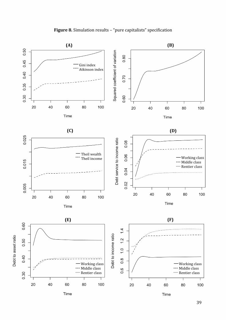
39
Figure 8. Simulation results – “pure capitalists” specification
(A) (B)
(C) (D)
(E) (F)
Gini index Atkinson index
Theil wealth Theil income Working class
Middle class Rentier class
Working class Middle class Rentier class
Working class Middle class Rentier class
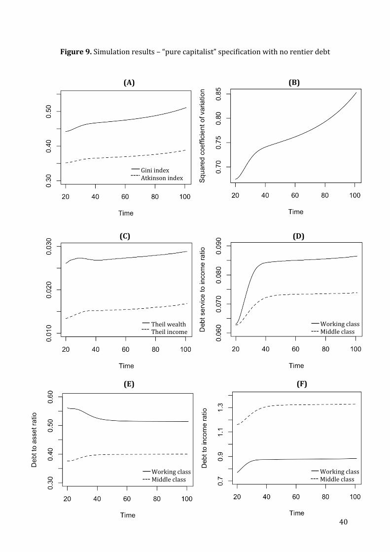
40
Figure 9. Simulation results – “pure capitalist” specification with no rentier debt
(A) (B)
(C) (D)
(E) (F)
Working class Middle class
Working class Middle class
Working class Middle class
Theil wealth Theil income
Gini index Atkinson index
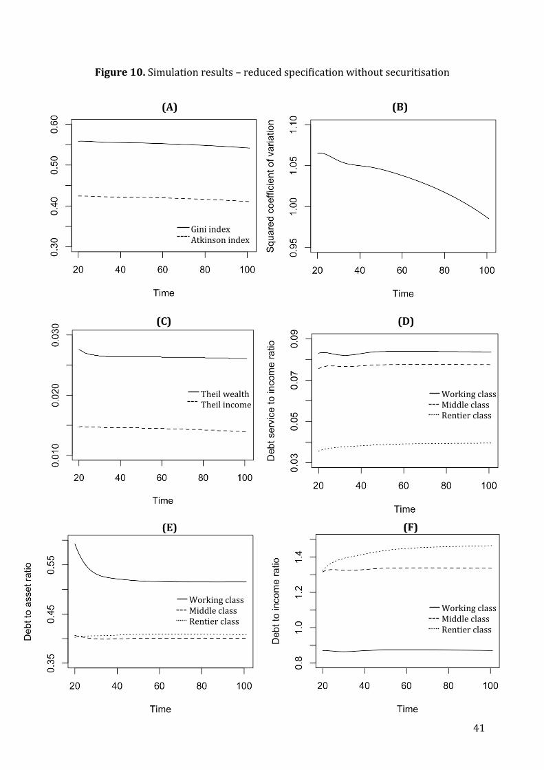
41
Figure 10. Simulation results – reduced specification without securitisation
(A) (B)
(C) (D)
(E) (F)
Theil wealth Theil income
Gini index Atkinson index
Working class Middle class Rentier class
Working class Middle class Rentier class
Working class Middle class Rentier class
42
VI. Conclusion and future work
Summary
The model outline presented here constitutes a first attempt of the author to
develop a theoretical model of inequality in the age of financialisation. SFCM is
adopted to account for the interactions between the financial and real sector and
their impact on the distribution of income and wealth in a financialised economy.
Unlike the existing functional distribution literature, in the current model
inequality is understood in terms of differential balance sheet and net wealth
structures among various income groups in the society. It is argued that this is a
more suitable approach to analysing inequality in times of financial sector
transformation as the traditionally envisaged groups of “workers” and
“capitalists” in the Post Keynesian literature became more heterogeneous since
1980s. While low- and middle-income households became actively involved in
financial markets through securitisation, the rich captured an increasing share of
income and economic power due to high returns to their wealth in result of
financial innovation and deregulation as well as high incomes received in the
financial sector. Thus, the innovation of our model is to reinterpret the groups of
workers and rentiers as well as to reconceptualise the middle class and its role in
inequality trends since 1980s.
The main distributional channels in our model emerge through credit
provision to the working and the middle class (firstly, because the interest
payments by the latter are ultimately received by the rentiers, and secondly,
because loans to the working and middle class are transformed into derivative
instruments held by rentiers); the housing sector (directly through rent
payments by the working class households to rentiers and indirectly through
interest payments on mortgages); and inequality is also reflected in the relative
consumption undertaken by the middle class.
Future work
At this early stage, the model is necessarily simplistic. In the near future, I aim to
extend the model so as to account for important processes influencing

43
distribution in the age of financial sector transformation, which could not be
considered at present due to their novelty and complexity.
The most innovative aspect which will be considered in the model is the
addition of more complex microeconomic behaviour using agent-based
modelling (ABM) techniques. The present SFCM representation is too aggregate
to study changes in the shape of the wealth and income distribution in detail.
This is because its macroeconomic character imposes a top-down structure of
behaviour in the model. This macroeconomic rigour is certainly important as
shown by Dafermos/Papatheodorou (2015) since aggregate mechanisms
provide important feedback mechanisms into the distribution of income, which
could give misleading outlook on the dynamics of inequality overtime if omitted.
However, it may not be a suitable starting point for the analysis of inequality
based on understanding what determines portfolio decisions of households and
hence their balance sheet structures in the times of financialisation. Agent-based
dynamics could inform what drives household behaviour when interacting with
different social groups, employers and the financial sector. It could also help to
correct the puzzle regarding the opposite than expected order of the debt-to-
income ratios in the present model.
In recent years, ABM has been propagated among economists as an
alternative to microfoundation development in macroeconomic theories, a
practice predominant in the paradigm of neoclassical general equilibrium
economics (cf. Gaffeo et al. 2007, Delli Gatti et al. 2011). ABM uses simulations to
analyse complex decentralised dynamic systems of interacting agents and de
facto construct economic states from the bottom-up. The key idea behind this
method is that the system is more than just a sum of its parts (Carvalho/Di
Giulmi 2013:3) and that the “fundamental social structures and aggregate
behaviors emerge from the interaction of individual agent operating on artificial
environments under rules that place only bounded demands on each agent’s
information and computation capacity” (Epstein/Axtell 1996:6). This, however,
is associated with methodological individualism — a trait of neoclassical
economics according to which the behaviour of economic agents is determined
solely by their individual characteristics in isolation from social interactions.
44
This methodological assumption has been particularly heavily criticised among
Post Keynesians as it obscures the importance of social influence of economic
decision-making. Importantly, however, in ABM social structures and institutions
do generate feedback mechanisms influencing agent behaviour. Consequently,
agents’ decisions, characteristics and resources are dynamic and can change
overtime in result of social interactions (Impullitti/Rebmann 2002:4). Moreover,
no agent has global information and knowledge is gained at the local level. These
features of ABM can handle a scenario in which agents with the same
preferences and endowments face different welfare outcomes (ibid.). Hence,
there exist disequilibria at the local level, resulting in a statistical equilibrium in
the model as a whole — an equilibrium which is probabilistic so that the optimal
allocation of resources among agents can never be achieved in a Pareto sense (cf.
Foley 1994). Clearly, this makes ABM distinct from the dynamic stochastic
general equilibrium models despite the shared assumption of methodological
individualism.
Further issue with ABM is that due to the decentralised nature of the
modelled systems, there is no analytical definition of the relationship between
the micro- and macro-level of analysis (Carvalho/Di Giulmi 2013:3).
Consequently, no precise causality between the two can be defined. Thus,
integration of ABM into SFCM proposed for our model carries the advantage that
macrostructures are clearly defined. In this case, rather than modelling the exact
behaviour of each agent, probabilistic evolution of the agents’ states can be
examined and used to endogenously derive macroeconomic equations and
interpret the micro-macro level interactions meaningfully (ibid.:3-4).
Since my main interest is to understand what drives inequality in the age
of financial sector transformation by examining the determinants of household
balance sheet composition, ABM combined with SFCM provides a suitable tool to
model household portfolio decisions and feedback mechanisms arising from the
interaction between the micro- and macroeconomic behaviour. Moreover, it
could allow for changing states of agents in our model and movement of
households between different social groups in result of, e.g. default (movement
from middle- to working class) or inheritance (movement from middle- to upper
45
class, or a Piketty future?). Overall, the addition of agent-based behaviour to the
model could produce a richer analysis of the determinants on household balance
sheet structures and hence inequality.
Furthermore, I will analyse the influence of specific balance sheet
structures on income shares of different household groups. Decomposition
technique could be adopted to reveal which aspect of balance sheet inequality
has the biggest impact on distribution. This issue remains ambiguous in the
literature. While the Post Keynesian theories of inequality reviewed earlier
suggest that it is debt which exacerbates the distribution of income away from
workers, empirical studies often find that it is the asset side of the balance sheets
that contributes more to inequality (cf. Fredriksen 2012). Similar conclusion can
be drawn from Piketty, according to whom high capital income from assets held
by the top 1% drives economic inequality. The unique setout of our model would
be capable of testing these competing claims.
Further extension to the present model will concern the inclusion of
social transfers. This is particularly important in the recent years, as due to
stagnating incomes and worsening working conditions (due to globalisation,
privatisation and labour market liberalisation), many especially low income
households (corresponding to the working class in our model) rely increasingly
on social security in their income. Furthermore, it would shed light on how
different taxation policies influence inequality.
46
References
Alvaredo, F., Atkinson, A.B., Piketty, T. and Saez, E., The World Top
Incomes Database, http://topincomes.g-mond.parisschoolofeconomics.eu;
AMECO Database, European Commission. Available at:
http://ec.europa.eu/economy_finance/ameco/user/serie/SelectSerie.cfm
[Accessed: 3/08/2015];
Ampudia M., van Vlokhoven, H., and Zochowski, D. (2014) “Financial
fragility of euro area households”, Working paper 1737, European Central Bank;
Atkinson, A.B. and Brandolini, A. (2011) “On the identification of the
“middle class””, ECINEQ Working Paper 2011-217,
Bivens, J., Gould, E., Mishel, L. and Shierholz, H. (2014) “Raising America’s
Pay. Why It’s Our Central Economic Policy Challenge”, Economics Policy Institute
Briefing Paper #378;
Bhaduri, A., and Marglin, S. (1990) “Unemployment and the real wage: the
economic basis for contesting political ideologies”, Cambridge Journal of
Economics, 14, pp. 375-393;
Boushey, H., and Weller, C. (2008) “Has Growing Inequality Contributed to
Rising Household Economic Distress?”, Review of Political Economy, 20(1), pp. 1-
22;
Carvalho, L., Di Giulmi, C. (2013) “Macroeconomic instability and
microeconomic financial fragility: a stock-flow consistent approach with
heterogeneous agents”, Working paper;
Caverzasi, E. and Godin, A. (2013) “Stock-flow Consistent Modeling
through the Ages”, The Levy Economics Institute Working Paper No. 745;
Caverzasi, E. and Godin, A. (2015) “Financialization and the sub-prime
crisis: a Stock-Flow Consistent model”, Working paper;
Copeland, M. A. (1949) “Social Accounting for Money Flows”, The
Accounting Review, 24(3), pp. 254–264;
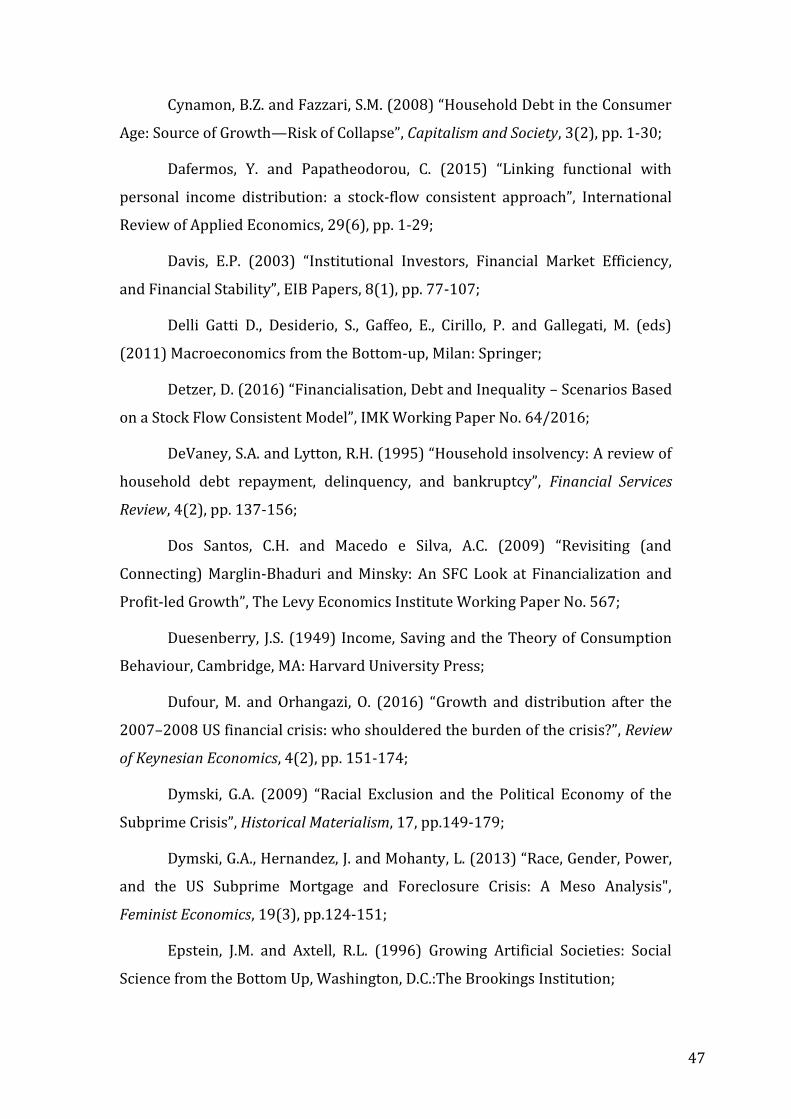
47
Cynamon, B.Z. and Fazzari, S.M. (2008) “Household Debt in the Consumer
Age: Source of Growth—Risk of Collapse”, Capitalism and Society, 3(2), pp. 1-30;
Dafermos, Y. and Papatheodorou, C. (2015) “Linking functional with
personal income distribution: a stock-flow consistent approach”, International
Review of Applied Economics, 29(6), pp. 1-29;
Davis, E.P. (2003) “Institutional Investors, Financial Market Efficiency,
and Financial Stability”, EIB Papers, 8(1), pp. 77-107;
Delli Gatti D., Desiderio, S., Gaffeo, E., Cirillo, P. and Gallegati, M. (eds)
(2011) Macroeconomics from the Bottom-up, Milan: Springer;
Detzer, D. (2016) “Financialisation, Debt and Inequality – Scenarios Based
on a Stock Flow Consistent Model”, IMK Working Paper No. 64/2016;
DeVaney, S.A. and Lytton, R.H. (1995) “Household insolvency: A review of
household debt repayment, delinquency, and bankruptcy”, Financial Services
Review, 4(2), pp. 137-156;
Dos Santos, C.H. and Macedo e Silva, A.C. (2009) “Revisiting (and
Connecting) Marglin-Bhaduri and Minsky: An SFC Look at Financialization and
Profit-led Growth”, The Levy Economics Institute Working Paper No. 567;
Duesenberry, J.S. (1949) Income, Saving and the Theory of Consumption
Behaviour, Cambridge, MA: Harvard University Press;
Dufour, M. and Orhangazi, O. (2016) “Growth and distribution after the
2007–2008 US financial crisis: who shouldered the burden of the crisis?”, Review
of Keynesian Economics, 4(2), pp. 151-174;
Dymski, G.A. (2009) “Racial Exclusion and the Political Economy of the
Subprime Crisis”, Historical Materialism, 17, pp.149-179;
Dymski, G.A., Hernandez, J. and Mohanty, L. (2013) “Race, Gender, Power,
and the US Subprime Mortgage and Foreclosure Crisis: A Meso Analysis",
Feminist Economics, 19(3), pp.124-151;
Epstein, J.M. and Axtell, R.L. (1996) Growing Artificial Societies: Social
Science from the Bottom Up, Washington, D.C.:The Brookings Institution;
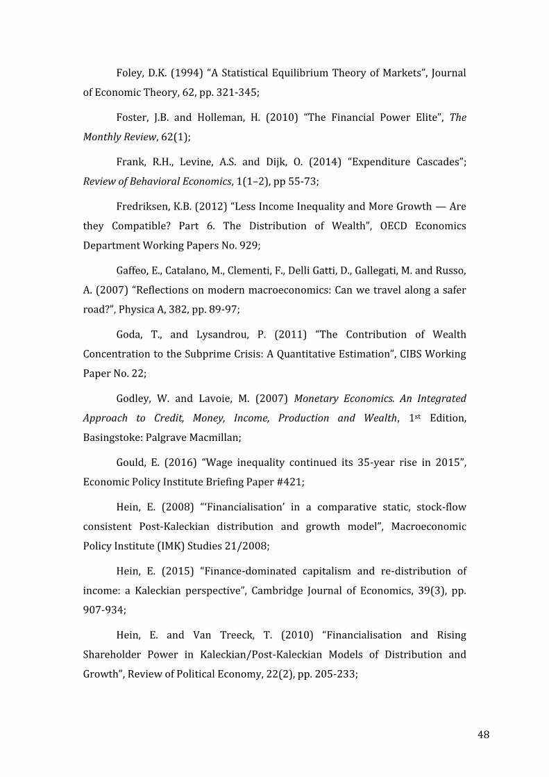
48
Foley, D.K. (1994) “A Statistical Equilibrium Theory of Markets”, Journal
of Economic Theory, 62, pp. 321-345;
Foster, J.B. and Holleman, H. (2010) “The Financial Power Elite”, The
Monthly Review, 62(1);
Frank, R.H., Levine, A.S. and Dijk, O. (2014) “Expenditure Cascades”;
Review of Behavioral Economics, 1(1–2), pp 55-73;
Fredriksen, K.B. (2012) “Less Income Inequality and More Growth — Are
they Compatible? Part 6. The Distribution of Wealth”, OECD Economics
Department Working Papers No. 929;
Gaffeo, E., Catalano, M., Clementi, F., Delli Gatti, D., Gallegati, M. and Russo,
A. (2007) “Reflections on modern macroeconomics: Can we travel along a safer
road?”, Physica A, 382, pp. 89-97;
Goda, T., and Lysandrou, P. (2011) “The Contribution of Wealth
Concentration to the Subprime Crisis: A Quantitative Estimation”, CIBS Working
Paper No. 22;
Godley, W. and Lavoie, M. (2007) Monetary Economics. An Integrated
Approach to Credit, Money, Income, Production and Wealth, 1st Edition,
Basingstoke: Palgrave Macmillan;
Gould, E. (2016) “Wage inequality continued its 35-year rise in 2015”,
Economic Policy Institute Briefing Paper #421;
Hein, E. (2008) “‘Financialisation’ in a comparative static, stock-flow
consistent Post-Kaleckian distribution and growth model”, Macroeconomic
Policy Institute (IMK) Studies 21/2008;
Hein, E. (2015) “Finance-dominated capitalism and re-distribution of
income: a Kaleckian perspective”, Cambridge Journal of Economics, 39(3), pp.
907-934;
Hein, E. and Van Treeck, T. (2010) “Financialisation and Rising
Shareholder Power in Kaleckian/Post-Kaleckian Models of Distribution and
Growth”, Review of Political Economy, 22(2), pp. 205-233;
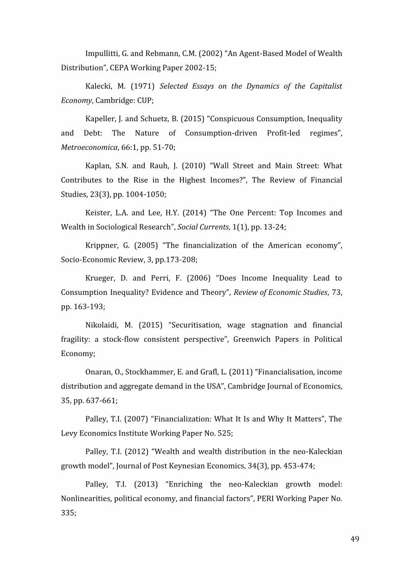
49
Impullitti, G. and Rebmann, C.M. (2002) “An Agent-Based Model of Wealth
Distribution”, CEPA Working Paper 2002-15;
Kalecki, M. (1971) Selected Essays on the Dynamics of the Capitalist
Economy, Cambridge: CUP;
Kapeller, J. and Schuetz, B. (2015) “Conspicuous Consumption, Inequality
and Debt: The Nature of Consumption-driven Profit-led regimes”,
Metroeconomica, 66:1, pp. 51-70;
Kaplan, S.N. and Rauh, J. (2010) “Wall Street and Main Street: What
Contributes to the Rise in the Highest Incomes?”, The Review of Financial
Studies, 23(3), pp. 1004-1050;
Keister, L.A. and Lee, H.Y. (2014) “The One Percent: Top Incomes and
Wealth in Sociological Research”, Social Currents, 1(1), pp. 13-24;
Krippner, G. (2005) “The financialization of the American economy”,
Socio-Economic Review, 3, pp.173-208;
Krueger, D. and Perri, F. (2006) “Does Income Inequality Lead to
Consumption Inequality? Evidence and Theory”, Review of Economic Studies, 73,
pp. 163-193;
Nikolaidi, M. (2015) “Securitisation, wage stagnation and financial
fragility: a stock-flow consistent perspective”, Greenwich Papers in Political
Economy;
Onaran, O., Stockhammer, E. and Grafl, L. (2011) “Financialisation, income
distribution and aggregate demand in the USA”, Cambridge Journal of Economics,
35, pp. 637-661;
Palley, T.I. (2007) “Financialization: What It Is and Why It Matters”, The
Levy Economics Institute Working Paper No. 525;
Palley, T.I. (2012) “Wealth and wealth distribution in the neo-Kaleckian
growth model”, Journal of Post Keynesian Economics, 34(3), pp. 453-474;
Palley, T.I. (2013) “Enriching the neo-Kaleckian growth model:
Nonlinearities, political economy, and financial factors”, PERI Working Paper No.
335;
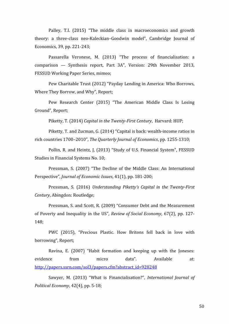
50
Palley, T.I. (2015) “The middle class in macroeconomics and growth
theory: a three-class neo-Kaleckian–Goodwin model”, Cambridge Journal of
Economics, 39, pp. 221-243;
Passarella Veronese, M. (2013) “The process of financialisation: a
comparison — Synthesis report, Part 3A", Version: 29th November 2013,
FESSUD Working Paper Series, mimeo;
Pew Charitable Trust (2012) “Payday Lending in America: Who Borrows,
Where They Borrow, and Why”, Report;
Pew Research Center (2015) “The American Middle Class Is Losing
Ground”, Report;
Piketty, T. (2014) Capital in the Twenty-First Century, Harvard: HUP;
Piketty, T. and Zucman, G. (2014) “Capital is back: wealth-income ratios in
rich countries 1700–2010”, The Quarterly Journal of Economics, pp. 1255-1310;
Pollin, R. and Heintz, J, (2013) “Study of U.S. Financial System", FESSUD
Studies in Financial Systems No. 10;
Pressman, S. (2007) “The Decline of the Middle Class: An International
Perspective”, Journal of Economic Issues, 41(1), pp. 181-200;
Pressman, S. (2016) Understanding Piketty’s Capital in the Twenty-First
Century, Abingdon: Routledge;
Pressman, S. and Scott, R. (2009) “Consumer Debt and the Measurement
of Poverty and Inequality in the US”, Review of Social Economy, 67(2), pp. 127-
148;
PWC (2015), “Precious Plastic. How Britons fell back in love with
borrowing”, Report;
Ravina, E. (2007) “Habit formation and keeping up with the Joneses:
evidence from micro data”. Available at:
http://papers.ssrn.com/sol3/papers.cfm?abstract_id=928248
Sawyer, M. (2013) “What is Financialisation?”, International Journal of
Political Economy, 42(4), pp. 5-18;
51
Sawyer, M. and Passarella Veronese, M. (2015) “The Monetary Circuit in
the age of Financialisation”, University of Leeds Working Paper;
Scott, R. and Pressman, S. (2015) “Inadequate Household Deleveraging:
Income, Debt and Social Provisioning”, Journal of Economic Issues, 49(2), pp. 483-
492;
Setterfield, M. and Kim, Y.K. (2013) “Debt Servicing, Aggregate
Consumption, and Growth”, Trinity College Department of Economics Working
Paper 13-16;
Survey of Consumer Finances, 1989-2013, Federal Reserve. Available at:
http://www.federalreserve.gov/econresdata/scf/scfindex.htm
Van Treeck, T. (2009) “A synthetic stock-flow consistent macroeconomic
model of financialisation”, Cambridge Journal of Economics, 33, pp. 467-493;
Veblen, T. (1899) The Theory of the Leisure Class, New York: Macmillan;
Wolff, E.N. (2014) “Household wealth trends in the United States, 1983-
2010”, Oxford Review of Economic Policy, 30(1), pp. 21-43.
World Bank (2005) “Inequality Measures”, Chapter 6, Poverty Manual;
Young, B. (2010) “The Gendered Dimension of Money, Finance and the
Subprime Crisis”. In: Bauhardt, C. and Caglar, G. (eds) Gender and Economics.
Feministische Kritik der politischen Oekonomie, Wiesbaden: VS Verlag für
Sozialwissenschaften;
Zezza, G. (2008) “U.S. growth, the housing market, and the distribution of
income”, Journal of Post Keynesian Economics, 30(3), pp. 375-401.
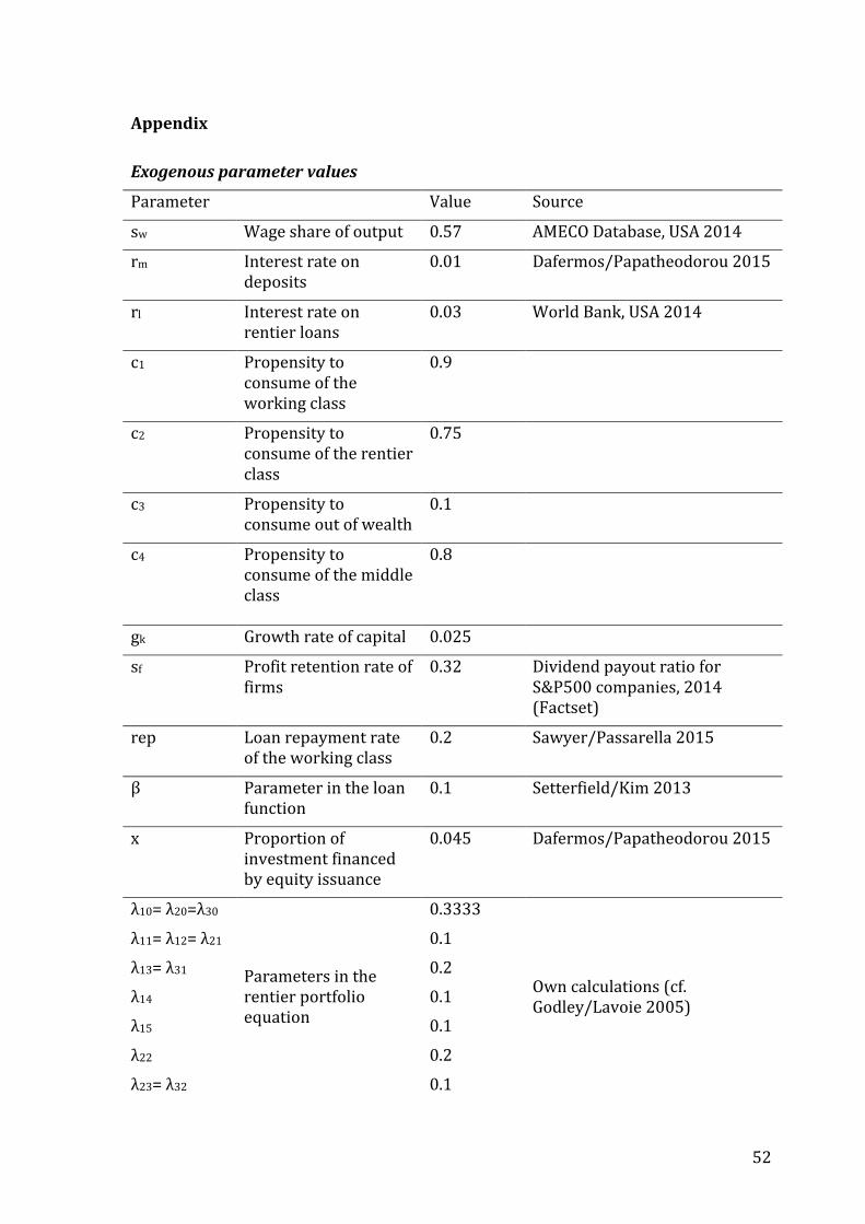
52
Appendix
Exogenous parameter values
Parameter Value Source
sw Wage share of output 0.57 AMECO Database, USA 2014
rm Interest rate on deposits
0.01 Dafermos/Papatheodorou 2015
rl Interest rate on rentier loans
0.03 World Bank, USA 2014
c1 Propensity to consume of the working class
0.9
c2 Propensity to consume of the rentier class
0.75
c3 Propensity to consume out of wealth
0.1
c4 Propensity to consume of the middle class
0.8
gk Growth rate of capital 0.025
sf Profit retention rate of firms
0.32 Dividend payout ratio for S&P500 companies, 2014 (Factset)
rep Loan repayment rate of the working class
0.2 Sawyer/Passarella 2015
β Parameter in the loan function
0.1 Setterfield/Kim 2013
x Proportion of investment financed by equity issuance
0.045 Dafermos/Papatheodorou 2015
λ10= λ20=λ30
Parameters in the rentier portfolio equation
0.3333
Own calculations (cf. Godley/Lavoie 2005)
λ11= λ12= λ21 0.1
λ13= λ31 0.2
λ14 0.1
λ15 0.1
λ22 0.2
λ23= λ32 0.1
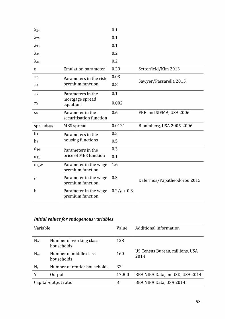
53
λ24 0.1
λ25 0.1
λ33 0.1
λ34 0.2
λ35 0.2
η Emulation parameter 0.29 Setterfield/Kim 2013
π0 Parameters in the risk premium function
0.03 Sawyer/Passarella 2015
π1 0.8
π2 Parameters in the mortgage spread equation
0.1
π3 0.002
s0 Parameter in the securitisation function
0.6 FRB and SIFMA, USA 2006
spreadMBS MBS spread 0.0121 Bloomberg, USA 2005-2006
h1 Parameters in the housing functions
0.5
h3 0.5
𝜃10 Parameters in the price of MBS function
0.3
𝜃11 0.1
m_w Parameter in the wage premium function
1.6
Dafermos/Papatheodorou 2015 𝜌 Parameter in the wage
premium function 0.3
h Parameter in the wage premium function
0.2/𝜌 + 0.3
Initial values for endogenous variables
Variable Value Additional information
Nw Number of working class households
128
US Census Bureau, millions, USA 2014
Nm Number of middle class households
160
Nr Number of rentier households 32
Y Output 17000 BEA NIPA Data, bn USD, USA 2014
Capital-output ratio 3 BEA NIPA Data, USA 2014
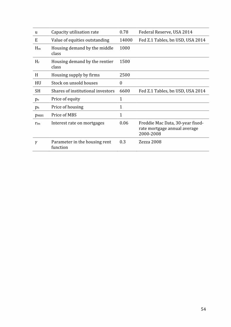
54
u Capacity utilisation rate 0.78 Federal Reserve, USA 2014
E Value of equities outstanding 14000 Fed Z.1 Tables, bn USD, USA 2014
Hm Housing demand by the middle class
1000
Hr Housing demand by the rentier class
1500
H Housing supply by firms 2500
HU Stock on unsold houses 0
SH Shares of institutional investors 6600 Fed Z.1 Tables, bn USD, USA 2014
pe Price of equity 1
ph Price of housing 1
pMBS Price of MBS 1
rlm Interest rate on mortgages 0.06 Freddie Mac Data, 30-year fixed-rate mortgage annual average 2000-2008
𝛾 Parameter in the housing rent function
0.3 Zezza 2008