INF1100 Lectures, Chapter 3:Functions and Branching

Hans Petter Langtangen

Simula Research Laboratory

University of Oslo, Dept. of Informatics

September 06, 2011

We have used many Python functions

Mathematical functions:from math import *y = sin(x)*log(x)

Other functions:n = len(somelist)ints = range(5, n, 2)

Functions used with the dot syntax (called methods):C = [5, 10, 40, 45]i = C.index(10) # result: i=1C.append(50)C.insert(2, 20)

What is a function? So far we have seen that we put someobjects in and sometimes get an object (result) out

Next topic: learn to write your own functions

Python functions

Function = a collection of statements we can executewherever and whenever we want

Function can take input objects and produce output objects

Functions help to organize programs, make them moreunderstandable, shorter, and easier to extend

Simple example: a mathematical function F (C ) = 95C + 32

def F(C):return (9.0/5)*C + 32

Functions start with def, then the name of the function, thena list of arguments (here C) – the function header

Inside the function: statements – the function body

Wherever we want, inside the function, we can ”stop thefunction” and return as many values/variables we want

Functions must be called

A function does not do anything before it is called

Examples on calling the F(C) function:a = 10F1 = F(a)temp = F(15.5)print F(a+1)sum_temp = F(10) + F(20)Fdegrees = [F(C) for C in Cdegrees]

Since F(C) produces (returns) a float object, we can call F(C)everywhere a float can be used

Local variables in Functions

Example: sum the integers from start to stop

def sumint(start, stop):s = 0 # variable for accumulating the sumi = start # counterwhile i <= stop:

s += ii += 1

return s

print sumint(0, 10)sum_10_100 = sumint(10, 100)

i and s are local variables in sumint – these are destroyed atthe end (return) of the function and never visible outside thefunction (in the calling program); in fact, start and stop arealso local variables

In the program above, there is one global variable, sum 10 100,and two local variables, s and i (in the sumint function)

Read Chapter 2.2.2 in the book about local and globalvariables!!

Python function for the ”ball in the air formula”

Recall the formula y(t) = v0t −12gt2:

We can make Python function for y(t):def yfunc(t, v0):

g = 9.81return v0*t - 0.5*g*t**2

# sample calls:y = yfunc(0.1, 6)y = yfunc(0.1, v0=6)y = yfunc(t=0.1, v0=6)y = yfunc(v0=6, t=0.1)

Functions can have as many arguments as you like

When we make a call yfunc(0.1, 6), all these statements arein fact executed:

t = 0.1 # arguments get values as in standard assignmentsv0 = 6g = 9.81return v0*t - 0.5*g*t**2

Functions may access global variables

The y(t,v0) function took two arguments

Could implement y(t) as a function of t only:>>> def yfunc(t):... g = 9.81... return v0*t - 0.5*g*t**2...>>> yfunc(0.6)...NameError: global name ’v0’ is not defined

v0 must be defined in the calling program program before wecall yfunc

>>> v0 = 5>>> yfunc(0.6)1.2342

v0 is a global variable

Global variables are variables defined outside functions

Global variables are visible everywhere in a program

g is a local variable, not visible outside of yfunc

Functions can return multiple values

Say we want to compute y(t) and y ′(t) = v0 − gt:def yfunc(t, v0):

g = 9.81y = v0*t - 0.5*g*t**2dydt = v0 - g*treturn y, dydt

# call:position, velocity = yfunc(0.6, 3)

Separate the objects to be returned by comma

What is returned is then actually a tuple>>> def f(x):... return x, x**2, x**4...>>> s = f(2)>>> s(2, 4, 16)>>> type(s)<type ’tuple’>>>> x, x2, x4 = f(2)

Example: compute a function defined as a sum

The function

L(x ; n) =

n∑

i=1

1

i

(

x

1 + x

)i

is an approximation to ln(1 + x) for a finite n and x ≥ 1

Let us make a Python function for L(x ; n):def L(x, n):

x = float(x) # ensure float division belows = 0for i in range(1, n+1):

s += (1.0/i)*(x/(1+x))**ireturn s

x = 5from math import log as lnprint L(x, 10), L(x, 100), ln(1+x)

Returning errors as well from the L(x, n) function

We can return more: also the first neglected term in the sumand the error (ln(1 + x)− L(x ; n)):

def L2(x, n):x = float(x)s = 0for i in range(1, n+1):

s += (1.0/i)*(x/(1+x))**ivalue_of_sum = sfirst_neglected_term = (1.0/(n+1))*(x/(1+x))**(n+1)from math import logexact_error = log(1+x) - value_of_sumreturn value_of_sum, first_neglected_term, exact_error

# typical call:x = 1.2; n = 100value, approximate_error, exact_error = L2(x, n)

Functions do not need to return objects

Let us make a table of L(x ; n) versus the exact ln(1 + x)

The table can be produced by a Python function

This function prints out text and numbers but do not need toreturn anything – we can then skip the final return

def table(x):print ’\nx=%g, ln(1+x)=%g’ % (x, log(1+x))for n in [1, 2, 10, 100, 500]:

value, next, error = L2(x, n)print ’n=%-4d %-10g (next term: %8.2e ’\

’error: %8.2e)’ % (n, value, next, error)

Output from table(10) on the screen:x=10, ln(1+x)=2.3979n=1 0.909091 (next term: 4.13e-01 error: 1.49e+00)n=2 1.32231 (next term: 2.50e-01 error: 1.08e+00)n=10 2.17907 (next term: 3.19e-02 error: 2.19e-01)n=100 2.39789 (next term: 6.53e-07 error: 6.59e-06)n=500 2.3979 (next term: 3.65e-24 error: 6.22e-15)

No return value implies that None is returned

Consider a function without any return value:>>> def message(course):... print "%s is the greatest fun I’ve "\... "ever experienced" % course...>>> message(’INF1100’)INF1100 is the greatest fun I’ve ever experienced>>> r = message(’INF1100) # store the return valueINF1100 is the greatest fun I’ve ever experienced>>> print rNone

None is a special Python object that represents an ”empty” orundefined value – we will use it a lot later

Keyword arguments

Functions can have arguments of the form name=value, calledkeyword arguments:

>>> def somefunc(arg1, arg2, kwarg1=True, kwarg2=0):>>> print arg1, arg2, kwarg1, kwarg2

>>> somefunc(’Hello’, [1,2]) # drop kwarg1 and kwarg2Hello [1, 2] True 0 # default values are used

>>> somefunc(’Hello’, [1,2], kwarg1=’Hi’)Hello [1, 2] Hi 0 # kwarg2 has default value

>>> somefunc(’Hello’, [1,2], kwarg2=’Hi’)Hello [1, 2] True Hi # kwarg1 has default value

>>> somefunc(’Hello’, [1,2], kwarg2=’Hi’, kwarg1=6)Hello [1, 2] 6 Hi # specify all args

If we use name=value for all arguments, their sequence can bearbitrary:

>>> somefunc(kwarg2=’Hello’, arg1=’Hi’, kwarg1=6, arg2=[2])Hi [2] 6 Hello

Example: function with default parameteres

Consider a function of t, with parameters A, a, and ω:

f (t;A, a, ω) = Ae−at sin(ωt)

We can implement f in a Python function with t as positionalargument and A, a, and ω as keyword arguments:

from math import pi, exp, sin

def f(t, A=1, a=1, omega=2*pi):return A*exp(-a*t)*sin(omega*t)

v1 = f(0.2)v2 = f(0.2, omega=1)v2 = f(0.2, 1, 3) # same as f(0.2, A=1, a=3)v3 = f(0.2, omega=1, A=2.5)v4 = f(A=5, a=0.1, omega=1, t=1.3)v5 = f(t=0.2, A=9)

Doc strings

Python convention: document the purpose of a function, itsarguments, and its return values in a doc string – a(triple-quoted) string written right after the function header

Examples:

def C2F(C):"""Convert Celsius degrees (C) to Fahrenheit."""return (9.0/5)*C + 32

def line(x0, y0, x1, y1):"""Compute the coefficients a and b in the mathematicalexpression for a straight line y = a*x + b that goesthrough two points (x0, y0) and (x1, y1).

x0, y0: a point on the line (floats).x1, y1: another point on the line (floats).return: a, b (floats) for the line (y=a*x+b)."""a = (y1 - y0)/(x1 - x0)b = y0 - a*x0return a, b

Convention for input and output data in functions

A function can have three types of input and output data:

input data specified through positional/keyword argumentsinput/output data given as positional/keyword arguments thatwill be modified and returnedoutput data created inside the function

All output data are returned, all input data are arguments

Sketch of a general Python function:def somefunc(i1, i2, i3, io4, io5, i6=value1, io7=value2):

# modify io4, io5, io7; compute o1, o2, o3return o1, o2, o3, io4, io5, io7

i1, i2, i3, i6: pure input data

io4, io5, io7: input and output data

o1, o2, o3: pure output data

The main program

A program contains functions and ordinary statements outsidefunctions, the latter constitute the main program

from math import * # in main

def f(x): # in maine = exp(-0.1*x)s = sin(6*pi*x)return e*s

x = 2 # in mainy = f(x) # in mainprint ’f(%g)=%g’ % (x, y) # in main

The execution starts with the first statement in the mainprogram and proceeds line by line, top to bottom

def statements define a function, but the statements insidethe function are not executed before the function is called

Math functions as arguments to Python functions

Programs doing calculus frequently need to have functions asarguments in other functions

We may have Python functions for

numerical integration:∫

b

af (x)dx

numerical differentiation: f ′(x)numerical root finding: f (x) = 0

Example: numerical computation of f ′′(x) by

f ′′(x) ≈f (x − h)− 2f (x) + f (x + h)

h2

def diff2(f, x, h=1E-6):r = (f(x-h) - 2*f(x) + f(x+h))/float(h*h)return r

No difficulty with f being a function (this is more complicatedin Matlab, C, C++, Fortran, and very much morecomplicated in Java)

Application of the diff2 function

Code:

def g(t):return t**(-6)

# make table of g’’(t) for 14 h values:for k in range(1,15):

h = 10**(-k)print ’h=%.0e: %.5f’ % (h, diff2(g, 1, h))

Output (g ′′(1) = 42):

h=1e-01: 44.61504h=1e-02: 42.02521h=1e-03: 42.00025h=1e-04: 42.00000h=1e-05: 41.99999h=1e-06: 42.00074h=1e-07: 41.94423h=1e-08: 47.73959h=1e-09: -666.13381h=1e-10: 0.00000h=1e-11: 0.00000h=1e-12: -666133814.77509h=1e-13: 66613381477.50939h=1e-14: 0.00000

What is the problem? Round-off errors...

For h < 10−8 the results are totally wrong

We would expect better approximations as h gets smaller

Problem: for small h we add and subtract numbers of approxequal size and this gives rise to round-off errors

Remedy: use float variables with more digits

Python has a (slow) float variable with arbitrary number ofdigits

Using 25 digits gives accurate results for h ≤ 10−13

Is this really a problem? Quite seldom – other uncertainies ininput data to a mathematical computation makes it usual tohave (e.g.) 10−2 ≤ h ≤ 10−6

If tests

Sometimes we want to peform different actions depending ona condition

Consider the function

f (x) =

{

sin x , 0 ≤ x ≤ π

0, otherwise

In a Python implementation of f we need to test on the valueof x and branch into two computations:

def f(x):if 0 <= x <= pi:

return sin(x)else:

return 0

In general (the else block can be skipped):if condition:

<block of statements, executed if condition is True>else:

<block of statements, executed if condition is False>

If tests with multiple branches (part 1)

We can test for multiple (here 3) conditions:if condition1:

<block of statements>elif condition2:

<block of statements>elif condition3:

<block of statements>else:

<block of statements><next statement>

If tests with multiple branches (part 2)

Example on multiple branches:

N(x) =

0, x < 0x , 0 ≤ x < 12− x , 1 ≤ x < 20, x ≥ 2

def N(x):if x < 0:

return 0elif 0 <= x < 1:

return xelif 1 <= x < 2:

return 2 - xelif x >= 2:

return 0

Inline if tests

A common construction isif condition:

variable = value1else:

variable = value2

This test can be placed on one line as an expression:variable = (value1 if condition else value2)

Example:def f(x):

return (sin(x) if 0 <= x <= 2*pi else 0)

Summary of if tests and functions

If tests:if x < 0:

value = -1elif x >= 0 and x <= 1:

value = xelse:

value = 1

User-defined functions:def quadratic_polynomial(x, a, b, c)

value = a*x*x + b*x + cderivative = 2*a*x + breturn value, derivative

# function call:x = 1p, dp = quadratic_polynomial(x, 2, 0.5, 1)p, dp = quadratic_polynomial(x=x, a=-4, b=0.5, c=0)

Positional arguments must appear before keyword arguments:def f(x, A=1, a=1, w=pi):

return A*exp(-a*x)*sin(w*x)

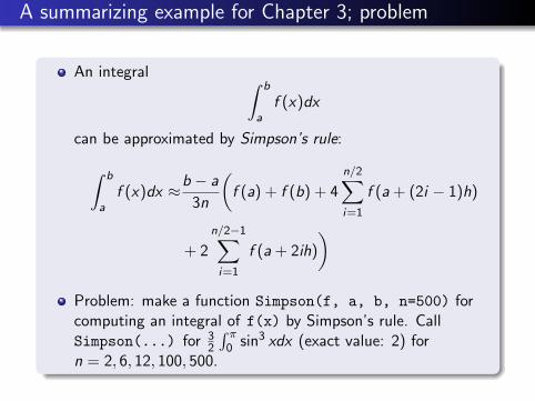
A summarizing example for Chapter 3; problem

An integral∫

b

a

f (x)dx

can be approximated by Simpson’s rule:

∫

b

a

f (x)dx ≈b − a

3n

(

f (a) + f (b) + 4

n/2∑

i=1

f (a+ (2i − 1)h)

+ 2

n/2−1∑

i=1

f (a+ 2ih)

)

Problem: make a function Simpson(f, a, b, n=500) forcomputing an integral of f(x) by Simpson’s rule. CallSimpson(...) for 3

2

∫ π0sin3 xdx (exact value: 2) for

n = 2, 6, 12, 100, 500.

The program: function for computing the formula

def Simpson(f, a, b, n=500):"""Return the approximation of the integral of ffrom a to b using Simpson’s rule with n intervals."""

h = (b - a)/float(n)

sum1 = 0for i in range(1, n/2 + 1):

sum1 += f(a + (2*i-1)*h)

sum2 = 0for i in range(1, n/2):

sum2 += f(a + 2*i*h)

integral = (b-a)/(3*n)*(f(a) + f(b) + 4*sum1 + 2*sum2)return integral

The program: function, now with test for possible errors

def Simpson(f, a, b, n=500):

if a > b:print ’Error: a=%g > b=%g’ % (a, b)return None

# Check that n is evenif n % 2 != 0:

print ’Error: n=%d is not an even integer!’ % nn = n+1 # make n even

# as before......return integral

The program: application (and main program)

def h(x):return (3./2)*sin(x)**3

from math import sin, pi

def application():print ’Integral of 1.5*sin^3 from 0 to pi:’for n in 2, 6, 12, 100, 500:

approx = Simpson(h, 0, pi, n)print ’n=%3d, approx=%18.15f, error=%9.2E’ %

application()

The program: verification

Property of Simpson’s rule: 2nd degree polynomials are integratedexactly!

def verify():"""Check that 2nd-degree polynomials are integrated exactly."""a = 1.5b = 2.0n = 8g = lambda x: 3*x**2 - 7*x + 2.5 # test integrandG = lambda x: x**3 - 3.5*x**2 + 2.5*x # integral of gexact = G(b) - G(a)approx = Simpson(g, a, b, n)if abs(exact - approx) > 1E-14: # never use == for floats!

print "Error: Simpson’s rule should integrate g exactly"

verify()