Statistical inference

Ian JolliffeIan Jolliffe

University of AberdeenUniversity of Aberdeen

CLIPS module 3.4CLIPS module 3.4bb

Probability and Statistics

Probability starts with a population, often Probability starts with a population, often described by a probability distribution, and described by a probability distribution, and predicts what will happen in a sample from that predicts what will happen in a sample from that population.population.

Statistics starts with a sample of data, and Statistics starts with a sample of data, and describes the data informatively, or makes describes the data informatively, or makes inferences about the population from which the inferences about the population from which the sample was drawn. sample was drawn.

This module concentrates on the inferential, rather This module concentrates on the inferential, rather than descriptive, side of Statistics.than descriptive, side of Statistics.

Probability vs. Statistics: an example

Probability: suppose we know that the Probability: suppose we know that the maximum temperature at a particular station maximum temperature at a particular station has a Gaussian distribution with mean 27has a Gaussian distribution with mean 27o o C C and standard deviation 3and standard deviation 3o o C. We can use this C. We can use this (population) probability distribution to (population) probability distribution to make predictions about the maximum make predictions about the maximum temperature on one or more days.temperature on one or more days.

Probability vs. Statistics: an example II

Statistics: for a new station we may wish to Statistics: for a new station we may wish to estimate the long-term (population) mean estimate the long-term (population) mean maximum temperature, and its standard maximum temperature, and its standard deviation, based on the small amount of deviation, based on the small amount of relevant data collected so far.relevant data collected so far.

Three types of statistical inference

Point estimation: given a sample of relevant data Point estimation: given a sample of relevant data find an estimate of the (population) mean find an estimate of the (population) mean maximum temperature in June at a station? Or an maximum temperature in June at a station? Or an estimate of the (population) probability of estimate of the (population) probability of precipitation in October at a station?precipitation in October at a station?

Interval estimation: given a sample of relevant Interval estimation: given a sample of relevant data, find a range of values within which we have data, find a range of values within which we have a high degree of confidence that the mean a high degree of confidence that the mean maximum temperature (or the probability of maximum temperature (or the probability of precipitation) liesprecipitation) lies

Three types of statistical inference II

Hypothesis testing: given a sample of Hypothesis testing: given a sample of relevant data, test one or more specific relevant data, test one or more specific hypotheses about the population from hypotheses about the population from which the sample is drawn. For example, is which the sample is drawn. For example, is the mean maximum temperature in June the mean maximum temperature in June higher at Station A than at Station B? Is the higher at Station A than at Station B? Is the daily probability of precipitation at Station daily probability of precipitation at Station A in October larger or smaller than 0.5?A in October larger or smaller than 0.5?

Representative samples

In the previous two Slides we have used the In the previous two Slides we have used the phrase ‘sample of relevant data’phrase ‘sample of relevant data’

It is crucial that the sample of data you use to It is crucial that the sample of data you use to make inferences about a population is make inferences about a population is representative of that population; otherwise the representative of that population; otherwise the inferences will be be biasedinferences will be be biased

Designing the best way of taking a sample is a Designing the best way of taking a sample is a third (as well as description and inference) aspect third (as well as description and inference) aspect of Statistics. It is important, but it will not be of Statistics. It is important, but it will not be discussed further in this modulediscussed further in this module

Estimates and errors

The need for probability and statistics arises The need for probability and statistics arises because nearly all measurements are subject to because nearly all measurements are subject to random variationrandom variation

One part of that random variation may be One part of that random variation may be measurement errormeasurement error

By taking repeated measurements of the same By taking repeated measurements of the same quantity we can quantify the measurement error –quantity we can quantify the measurement error – build a probability distribution for it, thenbuild a probability distribution for it, then use the distribution to find a ‘confidence interval’ for use the distribution to find a ‘confidence interval’ for

the ‘true’ value of the measurementthe ‘true’ value of the measurement

Confidence intervals

A point estimate on its own is of little useA point estimate on its own is of little use For example, if I tell you the probability of For example, if I tell you the probability of

precipitation tomorrow is 0.4, you will not know precipitation tomorrow is 0.4, you will not know how to react. Your reaction will be different if I how to react. Your reaction will be different if I then saythen say the probability is 0.4 +/- 0.01the probability is 0.4 +/- 0.01 the probability is 0.4 +/- 0.3the probability is 0.4 +/- 0.3

We need some indication of the precision of an We need some indication of the precision of an estimate, which leads naturally into confidence estimate, which leads naturally into confidence intervalsintervals

Confidence intervals II

The two statements on the previous slides were of The two statements on the previous slides were of the form ‘estimate +/- error’the form ‘estimate +/- error’

They could also be written as intervalsThey could also be written as intervals0.4 +/- 0.01 0.4 +/- 0.01 ( 0.39, 0.41) ( 0.39, 0.41)0.4 +/- 0.3 0.4 +/- 0.3 ( 0.10, 0.70) ( 0.10, 0.70)

For these intervals to be ‘confidence’ intervals we For these intervals to be ‘confidence’ intervals we need to associate a level of confidence with them need to associate a level of confidence with them – for example we might say that we are 95% – for example we might say that we are 95% confident that the interval includes the true confident that the interval includes the true probabilityprobability

Confidence intervals for what?

Confidence intervals can be found for any Confidence intervals can be found for any parameter or parameters (a quantity parameter or parameters (a quantity describing some aspect of a population or describing some aspect of a population or probability distribution).probability distribution).

Examples include Examples include probability of success in a binomial experimentprobability of success in a binomial experiment mean of a normal distributionmean of a normal distribution mean of a Poisson distributionmean of a Poisson distribution

…for what II?

More parametersMore parameters Differences between normal meansDifferences between normal means Differences between binomial probabilitiesDifferences between binomial probabilities Ratios of normal variancesRatios of normal variances Parameters describing Weibull, gamma or Parameters describing Weibull, gamma or

lognormal distributionslognormal distributions

Calculation of confidence intervals

No algebraic details are given, just the general No algebraic details are given, just the general principles behind most formulae for confidence principles behind most formulae for confidence intervalsintervals Find an estimate of the parameter of interestFind an estimate of the parameter of interest The estimate is a function of the data, so is a random The estimate is a function of the data, so is a random

variable, and hence has a probability distributionvariable, and hence has a probability distribution Use this distribution to construct probability statements Use this distribution to construct probability statements

about the estimateabout the estimate Manipulate the probability statements to turn them into Manipulate the probability statements to turn them into

statements about confidence intervals and their statements about confidence intervals and their coveragecoverage

Calculation of confidence intervals – an outline example

Suppose we have n independent observations on a Suppose we have n independent observations on a Gaussian random variable (for example maximum Gaussian random variable (for example maximum daily temperature in June). We write Udaily temperature in June). We write Ui i ~ ~

N(N(i = 1,2, …, n, where is the mean of the distribution and 2 is its variance

The sample mean, or average, of the n observations is an obvious estimator for . We denote this average by Ū, and it can be shown that Ū ~ N(n)

Confidence interval calculations II

Let Z = Let Z = √ n( n(Ū - μ)/σ. Then Z ~ N(0,1) We have tables of probabilities for N(0,1)

and can use these to make statements such as P( -1.96 < Z < 1.96 ) = 0.95 P( -2.58 < Z < 2.58 ) = 0.99 P (-1.65 < Z < 1.65 ) = 0.90

Probabilities for N(0,1) – 90% interval

-1.645 1.645

0.0

0.1

0.2

0.3

0.4

z

f(z)

Numbers indicate areas under curve, left of -1.65, right of 1.65, and between.

0.05

0.90

0.05

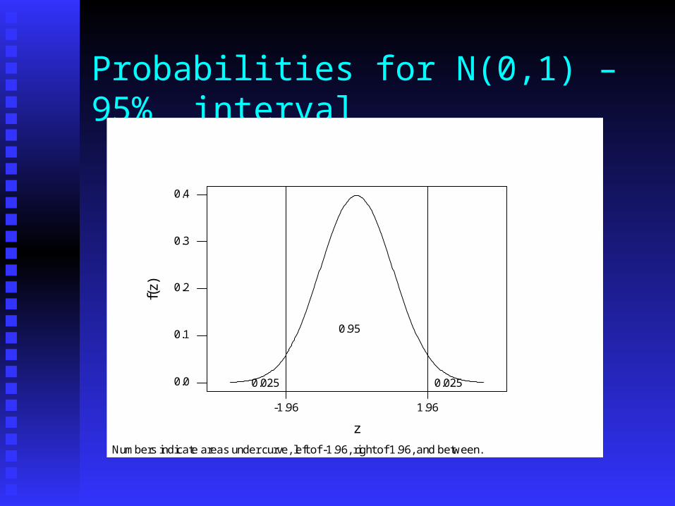
Probabilities for N(0,1) – 95% interval

-1.96 1.96

0.0

0.1

0.2

0.3

0.4

z

f(z)

Numbers indicate areas under curve, left of -1.96, right of 1.96, and between.

0.025

0.95

0.025

Confidence interval calculations III

Substituting the expression above for Z, in terms Substituting the expression above for Z, in terms of Ū, μ, σ and n, into the probability statements, of Ū, μ, σ and n, into the probability statements, and manipulating those statements givesand manipulating those statements gives P(P( ŪŪ -- 1.96σ/√n1.96σ/√n << μμ < < ŪŪ + 1.96 + 1.96σσ//√√n ) = 0.95n ) = 0.95 P(P( ŪŪ -- 2.58 2.58σ/√nσ/√n << μμ < < ŪŪ + 2.58 + 2.58σσ//√√n ) = 0.99n ) = 0.99 P(P( ŪŪ -- 1.65 1.65σ/√nσ/√n << μμ < < ŪŪ + 1.65 + 1.65σσ//√√n ) = 0.90n ) = 0.90

The intervals defined by these 3 expressions are The intervals defined by these 3 expressions are 95%, 99%, 90% confidence intervals respectively 95%, 99%, 90% confidence intervals respectively for μfor μ

Confidence interval for μ -example

Measurements are taken of maximum temperature at a Measurements are taken of maximum temperature at a station for a sample of 20 June days. Find a confidence station for a sample of 20 June days. Find a confidence interval for interval for μ, the (population) mean of maximum daily temperatures in June at that station.

The data give Ū = 25.625, and we assume that σ = 1.5. Substituting these values in the expressions on the

previous Slide gives 90% interval (25.07, 26.18) 95% interval (24.97, 26.28) 99% interval (24.76, 26.49)

Comments on confidence interval example Note how we ‘pay for’ a greater degree of confidence with Note how we ‘pay for’ a greater degree of confidence with

a wider interval a wider interval We have deliberately chosen the simplest possible We have deliberately chosen the simplest possible

example of a confidence interval – though intervals for example of a confidence interval – though intervals for other parameters (see Slides 11, 12) have similar other parameters (see Slides 11, 12) have similar constructions, most are a bit more complicated in detailconstructions, most are a bit more complicated in detail

One immediate complication is that we rarely know One immediate complication is that we rarely know σσ – it – it is replaced by an estimate, s, the sample standard is replaced by an estimate, s, the sample standard deviation. This leads to an interval which is based on a so-deviation. This leads to an interval which is based on a so-called t-distribution rather than N(0,1), and which is called t-distribution rather than N(0,1), and which is usually wider. usually wider.

Confidence interval example – more comments As well as assuming As well as assuming σσ known, the interval known, the interval

has also assumed normality (it needs to be has also assumed normality (it needs to be checked whether this assumption is OK), checked whether this assumption is OK), and independence of observations, which and independence of observations, which won’t be true if the data are recorded on won’t be true if the data are recorded on consecutive days in the same monthconsecutive days in the same month

Interpretation of confidence intervals

Interpretation is subtle/tricky and often Interpretation is subtle/tricky and often found difficult or misunderstoodfound difficult or misunderstood

A confidence interval is not a probability A confidence interval is not a probability statement about the chance of a (random) statement about the chance of a (random) parameter falling in a (fixed) intervalparameter falling in a (fixed) interval

It is a statement about the chance that a It is a statement about the chance that a random interval covers a fixed, but random interval covers a fixed, but unknown, parameterunknown, parameter

Hypothesis testing -introduction

For any parameter(s) where a confidence interval For any parameter(s) where a confidence interval can be constructed, it may also be of interest to can be constructed, it may also be of interest to test a hypothesis.test a hypothesis.

For simplicity, we develop the ideas of hypothesis For simplicity, we develop the ideas of hypothesis testing for the same scenario as our confidence testing for the same scenario as our confidence interval example, namely inference for interval example, namely inference for μ, a single , a single Gaussian mean, when Gaussian mean, when σ is known, though is known, though hypothesis testing is often more relevant when hypothesis testing is often more relevant when comparing two or more parameterscomparing two or more parameters

Hypothesis testing - example

Suppose that the instrument or exposure for Suppose that the instrument or exposure for measuring temperature has changed. Over a long measuring temperature has changed. Over a long period with the old instrument/ exposure, the period with the old instrument/ exposure, the mean value of daily June maximum temperature mean value of daily June maximum temperature was 25was 25ooC, with standard deviation 1.5C, with standard deviation 1.5ooCC

The data set described on Slide 19 comprises 20 The data set described on Slide 19 comprises 20 daily measurements with the new instrument/ daily measurements with the new instrument/ exposure. Is there any evidence of a change in exposure. Is there any evidence of a change in mean?mean?

The steps in hypothesis testing

1.1. Formulate a null hypothesis. The null hypothesis is Formulate a null hypothesis. The null hypothesis is often denoted as Hoften denoted as H00. In our example we have H. In our example we have H00: : μμ = 25= 25

2.2. Define a test statistic, a quantity which can be Define a test statistic, a quantity which can be computed from the data, and which will tend to computed from the data, and which will tend to take different values when Htake different values when H00 is true/false. is true/false. ŪŪ is an is an obvious estimator of obvious estimator of μμ, which should vary as , which should vary as μμ varies, and so is suitable as a test statistic. Z (see varies, and so is suitable as a test statistic. Z (see Slide 15) is equivalent to Slide 15) is equivalent to ŪŪ, and is more , and is more convenient, as its distribution is tabulated. Thus convenient, as its distribution is tabulated. Thus use Z as our test statistic.use Z as our test statistic.

Hypothesis testing steps II

33. Calculate the value of Z for the data.. Calculate the value of Z for the data.

Here Z = Here Z = √ n( n(Ū - μ)/σ, and Z ~ N(0,1). Assuming σ = 1.5, and the null value μ =25, we have Z = √20 (25.565 – 25) / 1.5 = 1.864. Calculate the probability of obtaining a value of the test

statistic at least as extreme as that observed, if the null hypothesis is true. This probability is called a p-value. Here we calculate P( Z > 1.86) if we believe before seeing the data that the change in mean temperature could only be an increase, or P(Z > 1.86) + P(Z < -1.86), if we believe the change could be in either direction.

Hypothesis testing steps III

The p-values are calculated from tables of the cumulative The p-values are calculated from tables of the cumulative distribution of N(0,1). From such tables, P( Z > 1.86 ) = distribution of N(0,1). From such tables, P( Z > 1.86 ) = 0.03, and because and symmetry of N(0,1) about zero, P 0.03, and because and symmetry of N(0,1) about zero, P ( Z < -1.86 ) = 0.03, and the two-sided p-value is 0.06( Z < -1.86 ) = 0.03, and the two-sided p-value is 0.06

Whether we calculate a one- or two-sided p-value depends Whether we calculate a one- or two-sided p-value depends on the context. If felt certain, before collecting the data, on the context. If felt certain, before collecting the data, that the change in instrument/exposure could only increase that the change in instrument/exposure could only increase mean temperature, a one-sided p-value is appropriate. mean temperature, a one-sided p-value is appropriate. Otherwise we should use the two-sided (two-tailed) valueOtherwise we should use the two-sided (two-tailed) value

Confidence intervals and hypothesis testing There is often, though not always, an There is often, though not always, an

equivalence between confidence intervals equivalence between confidence intervals and hypothesis testingand hypothesis testing

A null hypothesis is rejected at the 5% (1%) A null hypothesis is rejected at the 5% (1%) if and only if the null value of the parameter if and only if the null value of the parameter lies outside a 95% (99%) confidence lies outside a 95% (99%) confidence interval interval

Hypothesis testing: p-values

We haven’t yet said what to do with our calculated p-valueWe haven’t yet said what to do with our calculated p-value A small p-value casts doubt on the plausibility of the null A small p-value casts doubt on the plausibility of the null

hypothesis, Hhypothesis, H00, but …, but … It is NOT equal to P(HIt is NOT equal to P(H00|data)|data) How small is ‘small’? Frequently a single threshold is set, How small is ‘small’? Frequently a single threshold is set,

often 0.05, 0.01 or 0.10 (5%, 1%, 10%), and Hoften 0.05, 0.01 or 0.10 (5%, 1%, 10%), and H00 is rejected is rejected when the p-value falls below the threshold (rejected at the when the p-value falls below the threshold (rejected at the 5%, 1%, 10% significance level).5%, 1%, 10% significance level).

It is more informative to quote a p-value than to conduct It is more informative to quote a p-value than to conduct the test a single threshold levelthe test a single threshold level

Confidence intervals and hypothesis testing There is often, though not always, an There is often, though not always, an

equivalence between confidence intervals equivalence between confidence intervals and hypothesis testingand hypothesis testing

A null hypothesis is rejected at the 5% (1%) A null hypothesis is rejected at the 5% (1%) if and only if the null value of the parameter if and only if the null value of the parameter lies outside a 95% (99%) confidence lies outside a 95% (99%) confidence intervalsintervals