Inferring interaction partners from protein sequences

Anne-Florence Bitbol,1, 2, 3, ∗ Robert S. Dwyer,4 Lucy J. Colwell,5, † and Ned S. Wingreen1, 4, ‡

1Lewis-Sigler Institute for Integrative Genomics, Princeton University, Princeton, NJ 08544, USA2Department of Physics, Princeton University, Princeton, NJ 08544, USA

3Sorbonne Universites, Universite Pierre et Marie Curie - Paris 6,CNRS, Laboratoire Jean Perrin (UMR 8237), F-75005, Paris, France

4Department of Molecular Biology, Princeton University, Princeton, NJ 08544, USA5Department of Chemistry, University of Cambridge,

Lensfield Road, Cambridge CB2 1EW, United Kingdom

Specific protein-protein interactions are crucial in the cell, both to ensure the formation and sta-bility of multi-protein complexes, and to enable signal transduction in various pathways. Functionalinteractions between proteins result in coevolution between the interaction partners, causing theirsequences to be correlated. Here we exploit these correlations to accurately identify which proteinsare specific interaction partners from sequence data alone. Our general approach, which employs apairwise maximum entropy model to infer couplings between residues, has been successfully used topredict the three-dimensional structures of proteins from sequences. Thus inspired, we introduce aniterative algorithm to predict specific interaction partners from two protein families whose membersare known to interact. We first assess the algorithm’s performance on histidine kinases and responseregulators from bacterial two-component signaling systems. We obtain a striking 0.93 true positivefraction on our complete dataset without any a priori knowledge of interaction partners, and we un-cover the origin of this success. We then apply the algorithm to proteins from ATP-binding cassette(ABC) transporter complexes, and obtain accurate predictions in these systems as well. Finally,we present two metrics that accurately distinguish interacting protein families from non-interactingones, using only sequence data.

SIGNIFICANCE

Specific protein-protein interactions play crucial rolesin the stability of multi-protein complexes and in signaltransduction. Thus, mapping these interactions is keyto a systems-level understanding of cells. Systematic ex-perimental identification of protein interaction partnersis still challenging. However, a large and rapidly grow-ing amount of sequence data is now available. Is it pos-sible to identify which proteins interact just from theirsequences? We propose an approach based on sequencecovariation, building on methods used with success topredict the three-dimensional structures of proteins fromsequences alone. Our method identifies specific interac-tion partners with high accuracy among the membersof several ubiquitous prokaryotic protein families, andprovides a way to predict protein-protein interactions di-rectly from sequence data.

INTRODUCTION

Many key cellular processes are carried out by inter-acting proteins. For instance, specific protein-protein in-teractions ensure proper signal transduction in various

∗ anne-florence.bitbol@upmc.fr† ljc37@cam.ac.uk; L.J.C. and N.S.W. contributed equally to this

work.‡ wingreen@princeton.edu

pathways. Hence, mapping specific protein-protein in-teractions is central to a systems-level understanding ofcells, and has broad applications to areas such as drugtargeting. High-throughput experiments have recentlyelucidated a substantial fraction of protein-protein inter-actions in a few model organisms [1], but such experi-ments remain challenging. Meanwhile, there has been anexplosion of available sequence data. Can we exploit thisabundant new sequence data to identify specific protein-protein interaction partners?

Specific interactions between proteins imply evolution-ary constraints on the interacting partners. For instance,mutation of a contact residue in one partner generally im-pairs binding, but may be compensated by a complemen-tary mutation in the other partner. This co-evolution ofinteraction partners results in correlations between theiramino-acid sequences. Similar correlations exist withinsingle proteins, for example between amino acids thatare in contact in the folded protein. However, the sim-ple fact of a correlation between residues in a multiplesequence alignment is only weakly predictive of a three-dimensional contact [2–4], as correlation can also stemfrom indirect effects. Fortunately, global statistical mod-els allow direct and indirect interactions to be disentan-gled [5–7]. In particular, the maximum entropy prin-ciple [8] specifies the least-structured global statisticalmodel consistent with the one- and two-point statisticsof an alignment [5]. This approach has recently beenused with success to determine three-dimensional pro-tein structures from sequences [9–11], to predict muta-tional effects [12–14], and to find residue contacts be-tween known interaction partners [7, 15–19]. Pairwise

2

maximum entropy models have also been used produc-tively in various other fields [20–26].

Here we present a pairwise maximum entropy approachthat uses sequence data to predict interaction partnersamong the paralogous genes belonging to two interactingprotein families. We use histidine kinases (HKs) and re-sponse regulators (RRs) from prokaryotic two-componentsignaling systems (Fig. 1A) as our main benchmark.Two-component systems constitute a major class of path-ways that enable bacteria to sense and respond to envi-ronment signals. Typically, a transmembrane HK sensesa signal, autophosphorylates, and transfers its phosphategroup to its cognate RR, which induces a cellular re-sponse [28]. Most HKs are encoded in operons togetherwith their cognate RR, so interaction partners are known,which enables us to assess performance. There are of-ten dozens of paralogs of HKs and RRs in each genome,making prediction of interaction partners from sequencesalone highly nontrivial.

To address this challenge, we developed an iterativepairing algorithm (IPA, Fig. 1) that pairs proteins basedon their effective interaction energies as predicted by apairwise maximum entropy model. At each iteration, thehighest-scoring predicted HK-RR pairs are incorporatedinto the concatenated sequence alignment from which themodel is built. This yields a major increase of predic-tive accuracy through progressive training of the model.First, we consider the case where the IPA starts with atraining set of known HK-RR partners. We obtain goodperformance even with few training pairs. Then, we showthat the IPA can make accurate predictions starting with-out any known pairings, as would be needed to predictnovel protein-protein interactions. We trace the origin ofthis success to the preferential recruitment of new correctpairs by those already in the concatenated alignment. Wealso demonstrate how multiple random initializations canbe leveraged to improve performance. We show that ouralgorithm works more generally by successfully applyingit to ATP-binding cassette (ABC) transporter proteins.Finally, we develop two IPA-based methods that distin-guish interacting protein families from non-interactingones, using only sequence data.

RESULTS

Iterative pairing algorithm (IPA)

We have developed an iterative method to predictinteraction partners among the paralogs of two pro-tein families in each species, using just their sequences(Fig. 1A,B). In each iteration (Fig. 1C; Materials andMethods), we compute correlations between residuesfrom a concatenated alignment (CA) of paired sequences.The initial CA is either built from a training set of correctprotein pairs, or made from random pairs, assuming noprior knowledge of interacting pairs. We then infer cou-plings for all residue pairs using a pairwise maximum en-

tropy model built from the CA using a mean-field approx-imation [9, 29]. We calculate the interaction energy forevery possible protein pair within each species, by sum-ming the inter-protein couplings assigned by the model.Such “energies” capture evolutionary correlations, andcorrelate to physical energies for lattice proteins [30]. Us-ing these interaction energies, we predict protein pairs(assuming one-to-one specific HK-RR interactions [28],Fig. 1D). We attribute a confidence score to each pre-dicted protein pair, using the energy gap between thispair and the next best alternative (Fig. 1E). The CAis then updated by including the highest-scoring proteinpairs, and the next iteration can begin. At each iteration,all pairs in the CA are re-selected based on confidencescores (except initial training pairs, if any), allowing forerror correction.

Unless otherwise specified in what follows, our re-sults were obtained on a standard dataset comprising5064 HK-RR pairs for which the correct pairings areknown from gene adjacency. Each species has on average〈mp〉 = 11.0 pairs, and at least two pairs (see Materialsand Methods).

Starting from known pairings

We begin by predicting interaction partners startingfrom a training set of known pairs. To implement this,we pick a random set of Nstart known HK-RR pairs fromour standard dataset, and the first IPA iteration uses thisconcatenated alignment (CA) to train the model. Weblind the pairings of the remaining test set, and predictthem. At each subsequent iteration n > 1, the CA usedto retrain the model contains the initial training pairsplus the (n− 1)Nincrement highest-scoring predicted pairsfrom the previous iteration (see Materials and Methods).

At the first iteration, the fraction of accurately pre-dicted HK-RR pairs (true positive (TP) fraction) de-pends strongly on Nstart, and is close to the random ex-pectation (0.09) for small training sets, ranging from 0.13at Nstart = 1 to 0.93 for Nstart = 2000 (Fig. 2, inset, bluecurve). The TP fraction increases with subsequent iter-ations (Fig. 2, main panel). Strikingly, the final TP frac-tion depends only weakly on Nstart. For Nstart = 1, theIPA achieves a final TP fraction of 0.84, a huge increasefrom the initial value of 0.13 (Fig. 2, inset, red curve).This demonstrates the power of iterating: incorporatinghigh-scoring predicted pairs progressively increases thepredictive accuracy of the model.

Starting without known pairings

Given the success of the IPA with very small train-ing sets, we next ask whether predictions can be madewithout any prior knowledge of interacting pairs. To testthis, we randomly pair each HK with an RR from thesame species, and use these 5064 random pairs to train

3

FIG. 1. Iterative pairing algorithm (IPA). (A) Surface representations of a histidine kinase dimer (HK, top) and a responseregulator (RR, bottom), from a co-crystal structure [27]; the HK-RR contacts in each molecule are highlighted in color. (B) Tocorrectly pair HKs and RRs in each species from their sequences alone, we start from multiple sequence alignments of HKs andRRs, including 64 amino acids from the HK and 112 from the RR. (C) Schematic of the main steps of the IPA. (D, E) Exampleof HK-RR pair assignment and ranking by energy gap for one species. (D) Color map of the matrix of HK-RR interactionenergies in E. coli K-12 MG1655 from the final iteration of the IPA performed on our standard dataset, with a training setof Nstart = 100 HK-RR pairs, and an increment step of Nincrement = 200 pairs. As in every IPA iteration and every species,the pair with the lowest interaction energy is selected first (here, HK 10 - RR 10, boxed in white), and this HK and RR areremoved from further consideration (black hatches). Then, the next pair with the lowest energy is chosen, and the process isrepeated until all HKs and RRs are paired. (E) Energy spectrum from (D), showing the interaction energies with all the HKsfor each RR, with the correct HK-RR pairs shown in red. The energy gap ∆E is shown for RR 10. A confidence score basedon the energy gap is used to rank all assigned HK-RR pairs, and this ranking is exploited in order to build the concatenatedalignment for the subsequent IPA iteration. See Materials and Methods for details.

the initial model. At each subsequent iteration n > 1,the CA is built just from the (n − 1)Nincrement highest-scoring pairs from the previous iteration (see SupportingInformation).

Fig. 3 shows the progression of the TP fraction for dif-ferent values of Nincrement. It increases in all cases, andthe iterative method performs best for small incrementsteps (Fig. 3, inset). The low–Nincrement limit of the fi-nal TP fraction is 0.84, identical to that obtained with asingle training pair (Fig. 2). This striking TP fraction of0.84 is attained without any prior knowledge of HK-RRinteractions: the IPA bootstraps its way toward high pre-dictivity. The low–Nincrement limit is almost reached forNincrement = 6; thus we generically use Nincrement = 6 toreduce computational time while retaining near-optimalperformance. The final TP fraction is robust with re-

spect to different initializations: for Nincrement = 6, itsstandard deviation (over 500 replicates) is 0.04. For thecomplete dataset (23,424 HK-RR pairs), the IPA yieldsa TP fraction of 0.93 with no training data (see below).

Training process

The ability to accurately predict interaction partnerswithout training data is surprising. To understand it,we examine the evolution of the model over iterations ofthe IPA. In a well-trained model, the residue pairs withthe largest couplings have been shown to correspond tocontacts in the protein complex [7, 16, 31]. Up to iter-ation ∼100 − 150 (with Nincrement = 6), models start-ing from random pairings do no better than chance at

4

FIG. 2. Fraction of predicted pairs that are true positives(TP fraction), for different training set sizes Nstart. Mainpanel: Progression of the TP fraction during iterations of theIPA. The TP fraction is plotted versus the effective numberof HK-RR pairs (Meff , see Supporting Information, Eq. S1)in the concatenated alignment, which includes Nincrement = 6additional pairs at each iteration. The IPA is performed onthe standard dataset, and all results are averaged over 50replicates that differ by the random choice of training pairs.Dashed line: Average TP fraction obtained for random HK-RR pairings. Inset: Initial and final TP fractions (at first andlast iteration) versus Nstart.

identifying contacts. Subsequently, they improve rapidlyand soon predict contacts nearly as well as models con-structed from correct pairs (Figs. 4 and S1A).

At early stages, the model, constructed from few al-most random HK-RR pairs, poorly predicts real contactsand correct HK-RR pairs. However, couplings associatedto residue pairs that occur in the CA increase, raising thescores of HK-RR pairs with high sequence similarity tothose already in the CA, and making them more likely tobe added to the CA. We thus examine sequence similar-ity between the HK-RR pairs in the CA in consecutiveiterations. Specifically, we consider two HK-RR pairs tobe “neighbors” if the sequence identity between the twoHKs and between the two RRs are both > 70%. We findthat sequence similarity is crucial in the early recruitmentof new HK-RR pairs to the CA (Fig. S1B).

Understanding the initial increase of the TP fractionrequires a further observation. In our standard dataset,among all possible, within-species HK-RR pairs, the av-erage number of neighbor pairs per correct HK-RR pairis 9.66, of which 99% are correct. In contrast, the aver-age number of neighbor pairs per incorrect HK-RR pairis 5.25, of which less than 1% are correct. Thus, correctpairs are more similar to each other than they are to in-correct pairs, or than incorrect pairs are to each other.We call this the Anna Karenina effect, in reference tothe first sentence of Tolstoy’s novel [32]: All happy fami-

FIG. 3. Starting from random pairings, i.e. without knownpairings. Main panel: TP fraction during iterations of theIPA versus the effective number of HK-RR pairs (Meff) in theconcatenated alignment, which includes Nincrement additionalpairs at each iteration. Different curves correspond to differ-ent Nincrement. The IPA is performed on the standard dataset,and all results are averaged over 50 replicates that differ intheir initial random pairings. Note that the first point of eachcurve corresponds to the second iteration. Dashed line: Aver-age TP fraction obtained for random HK-RR pairings. Inset:Final TP fraction versus Nincrement.

lies are alike; each unhappy family is unhappy in its ownway. Biologically, this makes sense: each HK-RR pair isan evolutionary unit, so a correct pair is likely to haveorthologs of both the HK and the RR in multiple otherspecies, whereas an incorrect pair is less likely to haveorthologs of both the HK and the (non-cognate) RR inother species. Hence, in early iterations, the number ofneighbors recruited per correct pair is higher than perwrong pair (Fig. S1B), increasing the TP fraction in theCA. To summarize, sequence similarity is crucial at earlystages, and the Anna Karenina effect helps to increasethe TP fraction in the CA, thus promoting training ofthe model. This suggests that the IPA might be furtherenhanced by initially scoring HK-RR pairs based on sim-ilarity [33].

Application of the IPA to ABC transporters

To demonstrate the utility of the IPA beyond HK-RRs, we applied it to several protein families involvedin ABC transporter complexes. Bacterial genomes typi-cally contain multiple paralogs of these transporters, in-volved in the translocation of different substances [34].We built alignments of homologs of the Escherichia coliinteracting protein pairs MALG-MALK, FBPB-FBPC,and GSIC-GSID (see Supporting Information). These

5

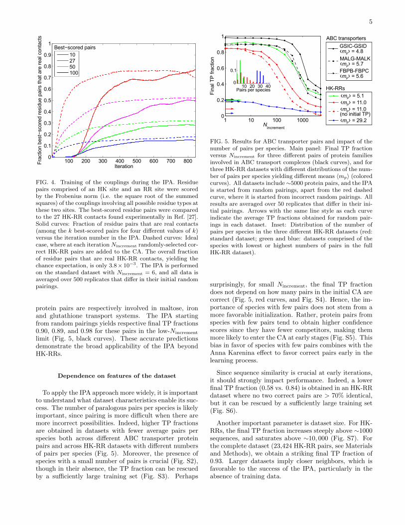
FIG. 4. Training of the couplings during the IPA. Residuepairs comprised of an HK site and an RR site were scoredby the Frobenius norm (i.e. the square root of the summedsquares) of the couplings involving all possible residue types atthese two sites. The best-scored residue pairs were comparedto the 27 HK-RR contacts found experimentally in Ref. [27].Solid curves: Fraction of residue pairs that are real contacts(among the k best-scored pairs for four different values of k)versus the iteration number in the IPA. Dashed curves: Idealcase, where at each iterationNincrement randomly-selected cor-rect HK-RR pairs are added to the CA. The overall fractionof residue pairs that are real HK-RR contacts, yielding thechance expectation, is only 3.8× 10−3. The IPA is performedon the standard dataset with Nincrement = 6, and all data isaveraged over 500 replicates that differ in their initial randompairings.

protein pairs are respectively involved in maltose, ironand glutathione transport systems. The IPA startingfrom random pairings yields respective final TP fractions0.90, 0.89, and 0.98 for these pairs in the low-Nincrement

limit (Fig. 5, black curves). These accurate predictionsdemonstrate the broad applicability of the IPA beyondHK-RRs.

Dependence on features of the dataset

To apply the IPA approach more widely, it is importantto understand what dataset characteristics enable its suc-cess. The number of paralogous pairs per species is likelyimportant, since pairing is more difficult when there aremore incorrect possibilities. Indeed, higher TP fractionsare obtained in datasets with fewer average pairs perspecies both across different ABC transporter proteinpairs and across HK-RR datasets with different numbersof pairs per species (Fig. 5). Moreover, the presence ofspecies with a small number of pairs is crucial (Fig. S2),though in their absence, the TP fraction can be rescuedby a sufficiently large training set (Fig. S3). Perhaps

FIG. 5. Results for ABC transporter pairs and impact of thenumber of pairs per species. Main panel: Final TP fractionversus Nincrement for three different pairs of protein familiesinvolved in ABC transport complexes (black curves), and forthree HK-RR datasets with different distributions of the num-ber of pairs per species yielding different means 〈mp〉 (coloredcurves). All datasets include∼5000 protein pairs, and the IPAis started from random pairings, apart from the red dashedcurve, where it is started from incorrect random pairings. Allresults are averaged over 50 replicates that differ in their ini-tial pairings. Arrows with the same line style as each curveindicate the average TP fractions obtained for random pair-ings in each dataset. Inset: Distribution of the number ofpairs per species in the three different HK-RR datasets (red:standard dataset; green and blue: datasets comprised of thespecies with lowest or highest numbers of pairs in the fullHK-RR dataset).

surprisingly, for small Nincrement, the final TP fractiondoes not depend on how many pairs in the initial CA arecorrect (Fig. 5, red curves, and Fig. S4). Hence, the im-portance of species with few pairs does not stem from amore favorable initialization. Rather, protein pairs fromspecies with few pairs tend to obtain higher confidencescores since they have fewer competitors, making themmore likely to enter the CA at early stages (Fig. S5). Thisbias in favor of species with few pairs combines with theAnna Karenina effect to favor correct pairs early in thelearning process.

Since sequence similarity is crucial at early iterations,it should strongly impact performance. Indeed, a lowerfinal TP fraction (0.58 vs. 0.84) is obtained in an HK-RRdataset where no two correct pairs are > 70% identical,but it can be rescued by a sufficiently large training set(Fig. S6).

Another important parameter is dataset size. For HK-RRs, the final TP fraction increases steeply above ∼1000sequences, and saturates above ∼10, 000 (Fig. S7). Forthe complete dataset (23,424 HK-RR pairs, see Materialsand Methods), we obtain a striking final TP fraction of0.93. Larger datasets imply closer neighbors, which isfavorable to the success of the IPA, particularly in theabsence of training data.

6

Optimization

To improve the predictive ability of the IPA, we ex-ploit multiple different random initializations of the CA.For each possible, within-species HK-RR pair, we calcu-late the fraction fr of replicates of the IPA in which thispair is predicted. High fr values are excellent predic-tors of correct pairs, outperforming average TP fractionsfrom individual replicates (Fig. S8). The quality of fras a classifier is demonstrated by the area under the re-ceiver operating characteristic: it is 0.991, very close to1 (ideal). The very high TP fraction of the pairs withhighest fr can be exploited by taking some as trainingpairs and running the IPA again. This “rebootstrapping”process can be iterated, yielding further performance in-creases, particularly for small datasets (Fig. S9).

Determining whether two protein families interact

The IPA correctly predicts most interacting proteinpairs no matter which initial random pairing is used.This suggests that the distribution of replication fractionsfr (over all possible within-species pairs) should distin-guish pairs of protein families that interact from thosethat do not. To test this idea, we consider three pairsof families with similar 〈mp〉: the subset of HK-RRs ho-mologous to BASS-BASR, the homologs of the interact-ing ABC transporter proteins MALG-MALK, and a pairwith no known interaction, homologs of BASR-MALK.For both interacting protein families, the distribution ofreplication fractions fr strongly favors values close to0, mostly corresponding to wrong pairs, and close to 1,mostly corresponding to correct pairs (Fig. 6A-B). Nosuch bimodality is observed for BASR-MALK (Fig. 6C).We constructed null models for each dataset by randomlyscrambling the amino acids at each site (column) of thealignment, thus retaining conservation while removingcorrelations. For BASR-MALK, the observed fr distribu-tion is very similar to the null-model distribution, whilefor both interacting pairs the results and the null stronglydiffer (Fig. 6). The standard HK-RR dataset can be sim-ilarly contrasted with an HK-RR dataset lacking correctpairs (Fig. S10). Comparing the observed fr distribu-tion to the null thus distinguishes interacting from non-interacting protein families using sequence data alone.For these family pairs, the difference in fr distributionsis visible down to dataset sizes M ∼500. Another sig-nature of interacting families is the strength of the toppredicted contacts (Fig. S11).

DISCUSSION

We have presented a method to infer interaction part-ners among two protein families with multiple paralogs,using only sequence data. Our approach is based on pair-wise maximum entropy models, which have proved suc-

FIG. 6. An IPA-derived signature of protein-protein inter-actions. For three pairs of protein families, we compute thefraction fr of IPA replicates in which each possible within-species protein pair is predicted as a pair. (A and B) Proteinfamilies with known interactions: (A) BASS-BASR homologsand (B) MALG-MALK homologs; (C) Protein families withno known interaction (BASR-MALK homologs). Red curves:Distribution of fr obtained for each alignment. Blue curves:Same distribution obtained by running the IPA on alignmentswhere each column is scrambled (null model). Alignments in-clude ∼5000 pairs, with 〈mp〉 ≈ 5, and each distribution isestimated from 500 IPA replicates that differ in their initialrandom pairings, using Nincrement = 50.

cessful at predicting residue contacts between known in-teraction partners [7, 15–19]. To our knowledge, the im-portant problem of predicting interaction partners amongparalogs from sequences has only been addressed byBurger and van Nimwegen [6], who used a Bayesiannetwork method. Pairwise maximum entropy-based ap-proaches were later shown to outperform this methodfor orphan HK-RR partner predictions, starting from asubstantial training set of partners known from gene ad-jacency [15]. Importantly, our method enables partnerprediction without any initial known pairs, whereas eventhe seminal study [6] included a training set via speciesthat contain only a single pair. This lack of a training setis important to predict novel protein-protein interactions,since in this context no prior knowledge of interactingpairs would be available.

We first benchmarked our iterative pairing algorithm(IPA) on HK-RR pairs. The top-scoring predicted HK-RR pairs are progressively incorporated into the con-catenated alignment used to build the maximum entropymodel. This enables progressive training of the model,providing major increases in predictive accuracy. Strik-ingly, the IPA is very successful even in the absence ofany prior knowledge of HK-RR interactions, yielding a0.93 TP fraction on our complete dataset. The successof the IPA with no training data relies on initial recruit-ment of pairs by sequence similarity. Correct pairs aremore similar to one another than incorrect pairs, favor-ing recruitment of correct pairs - a process we called the“Anna Karenina effect”.

IPA performance is best for large datasets (with strongsequence similarity), and when species with few pairs areincluded. The first condition is easily met for HK-RRs(a 0.84 TP fraction was obtained with 5064 pairs, out of23,424, and our rebootstrapping approach yields a 0.64

7

TP fraction even for a dataset of only 502 pairs, Fig. S9B)and is realized for a large and growing number of otherprotein families. Indeed, in the protein family databasePfamA-30 [35], 62% of the 15,701 entries classified as“domains” or “families” comprise more than 500 distinctUniprot sequences. The mean number of paralogs perspecies in PfamA-30 domains or families is 3.9, so theHK-RR system actually constitutes an unusually diffi-cult case in this respect [28]. The success we obtained forABC transporter proteins, which form permanent com-plexes, while HK-RRs interact transiently, further pointsto the broad applicability of the IPA. So far we haveonly applied the IPA to one-to-one interactions, but themethod should be fruitful beyond this domain.

Our approach could be combined with those of Refs. [7,13, 15–19] to improve protein complex structure predic-tion. It solves the major issue [17–19] of finding the cor-rect interaction partners among paralogs, which is a pre-requisite for accurate contact prediction. In particular,better paralog-partner predictions will help extend ac-curate contact prediction to currently-inaccessible casessuch as eukaryotic proteins, for which genome organiza-tion cannot be used to find partners.

Finally, we have introduced two distinct IPA-basedsignatures that distinguish between interacting and non-interacting protein families. These results pave the waytoward predicting novel protein-protein interactions be-tween protein families from sequence data alone.

MATERIALS AND METHODS

Extended Materials and Methods are presented in theSupporting Information.

HK-RR dataset

Our dataset was built from the P2CS database [36, 37],which includes two-component system proteins from allfully-sequenced prokaryotic genomes. All data can thusbe accessed online. We considered the protein domainsthrough which HKs and RRs interact, namely the PfamHisKA domain present in most HKs (64 amino acids)and the Pfam Response reg domain present in all RRs(112 amino acids). We focused on proteins with knownpartners, i.e. those encoded in the genome in pairs con-taining an HK and an adjacent RR. Discarding specieswith only one pair, for which pairing is unambiguous,we obtained a complete dataset of 23,424 HK-RR pairsfrom 2102 species. A smaller “standard dataset” of 5064pairs from 459 species was extracted by picking speciesrandomly.

Iterative pairing algorithm (IPA)

Here, we summarize each of the steps of an iterationof the IPA (Fig. 1C).1. Correlations. Each iteration begins by the cal-

culation of empirical correlations from the CA of pairedHK-RR sequences. The empirical one- and two-site fre-quencies, fi(α) and fij(α, β), of occurrence of amino-acidstates α (or β) at each site i (or j) are computed forthe CA, using a re-weighting of similar sequences, and apseudocount correction (Eqs. S1-S4) [7, 9, 15, 29]. Thecorrelations are then computed as

Cij(α, β) = fij(α, β)− fi(α)fj(β) . (1)

2. Couplings. Next, we construct a pairwise max-imum entropy model of the CA (Eq. S6). It involvesone-body fields hi at each site i and (direct) couplingseij between all sites i and j, which are determined byimposing consistency of the pairwise maximum entropymodel with the empirical one- and two-point frequenciesof the CA (Eqs. S7-S8). We use the mean-field approx-imation [9, 29]: couplings are obtained by inverting thematrix of correlations:

eij(α, β) = C−1ij (α, β) . (2)

We then transform to the zero-sum gauge [7, 31].3. Interaction energies for all possible HK-RR

pairs. The interaction energy E of each possible HK-RR pair within each species is calculated as a sum ofcouplings:

E (α1, ..., αLHK, αLHK+1, ..., αL) =

LHK∑i=1

L∑j=LHK+1

eij(αi, αj) ,

(3)where LHK denotes the length of the HK sequence andL that of the concatenated HK-RR sequence.4. HK-RR pair assignments and ranking by

gap. In each species, the pair with the lowest interactionenergy is selected first, and the HK and RR involved areremoved from further consideration, assuming one-to-oneHK-RR matches (Fig. 1D). Then, the pair with the nextlowest energy is chosen, until all HKs and RRs are paired.Each pair is scored at assignment by a confidence score∆E/(n+ 1), where ∆E is the energy gap (Fig. 1E), andn is the number of lower-energy matches discarded inassignments made previously, within that species and atthat iteration (Fig. S12). All the assigned HK-RR pairsare then ranked in order of decreasing confidence score.5. Incrementation of the CA. At each iteration

n > 1, the (n − 1)Nincrement assigned pairs that had thehighest confidence scores at iteration n − 1 are includedin the CA. In the presence of an initial training set, theNstart training pairs are also included in the CA. Withouta training set, the initial CA is built by randomly pairingeach HK of the dataset to an RR from the same species,and for n > 1, the CA only contains the above-mentioned(n − 1)Nincrement assigned pairs. Once the new CA isconstructed, the next iteration can start.

8

ACKNOWLEDGMENTS

We thank Mohamed Barakat and Philippe Ortet forsharing and discussing specifically-formatted datasetsbuilt from the P2CS database. AFB acknowledgessupport from the Human Frontier Science Program.This research was supported in part by NIH GrantR01-GM082938 (AFB and NSW) and by NSF GrantPHY1305525 (NSW), Marie Curie Career IntegrationGrant 631609 (LJC), a Next Generation Fellowship(LJC), and the Eric and Wendy Schmidt TransformativeTechnology Fund.

AUTHOR CONTRIBUTIONS

A.F.B., R.S.D., L.J.C. and N.S.W. designed research,A.F.B., L.J.C. and N.S.W. performed research, analyzeddata, and wrote the paper.

NOTE

While submitting this manuscript, we learned that T.Gueudre, C. Baldassi, M. Zamparo, M. Weigt, and A.Pagnani are preparing a related paper on predicting in-teracting paralog pairs.

[1] Rajagopala SV et al. (2014) The binary protein-proteininteraction landscape of Escherichia coli. Nat. Biotech-nol. 32(3):285–290.

[2] Altschuh D, Lesk AM, Bloomer AC, Klug A (1987) Cor-relation of co-ordinated amino acid substitutions withfunction in viruses related to tobacco mosaic virus. J.Mol. Biol. 193(4):693–707.

[3] Lockless SW, Ranganathan R (1999) Evolutionarily con-served pathways of energetic connectivity in protein fam-ilies. Science 286(5438):295–299.

[4] Skerker JM et al. (2008) Rewiring the specificityof two-component signal transduction systems. Cell133(6):1043–1054.

[5] Lapedes AS, Giraud BG, Liu L, Stormo GD (1999) Cor-related mutations in models of protein sequences: phy-logenetic and structural effects in Statistics in molecularbiology and genetics - IMS Lecture Notes - MonographSeries. Vol. 33, pp. 236–256.

[6] Burger L, van Nimwegen E (2008) Accurate predictionof protein-protein interactions from sequence alignmentsusing a Bayesian method. Mol. Syst. Biol. 4:165.

[7] Weigt M, White RA, Szurmant H, Hoch JA, Hwa T(2009) Identification of direct residue contacts in protein-protein interaction by message passing. Proc. Natl. Acad.Sci. U.S.A. 106(1):67–72.

[8] Jaynes ET (1957) Information Theory and StatisticalMechanics. Phys. Rev. 106(4):620–630.

[9] Marks DS et al. (2011) Protein 3D structure com-puted from evolutionary sequence variation. PLoS ONE6(12):e28766.

[10] Su lkowska JI, Morcos F, Weigt M, Hwa T, Onuchic JN(2012) Genomics-aided structure prediction. Proc. Natl.Acad. Sci. U.S.A. 109(26):10340–10345.

[11] Jones DT, Buchan DW, Cozzetto D, Pontil M (2012)PSICOV: precise structural contact prediction usingsparse inverse covariance estimation on large multiple se-quence alignments. Bioinformatics 28(2):184–190.

[12] Dwyer RS, Ricci DP, Colwell LJ, Silhavy TJ, WingreenNS (2013) Predicting functionally informative mutationsin Escherichia coli BamA using evolutionary covarianceanalysis. Genetics 195(2):443–455.

[13] Cheng RR, Morcos F, Levine H, Onuchic JN (2014) To-ward rationally redesigning bacterial two-component sig-naling systems using coevolutionary information. Proc.Natl. Acad. Sci. U.S.A. 111(5):E563–571.

[14] Figliuzzi M, Jacquier H, Schug A, Tenaillon O, WeigtM (2016) Coevolutionary Landscape Inference and theContext-Dependence of Mutations in Beta-LactamaseTEM-1. Mol. Biol. Evol. 33(1):268–280.

[15] Procaccini A, Lunt B, Szurmant H, Hwa T, Weigt M(2011) Dissecting the specificity of protein-protein in-teraction in bacterial two-component signaling: orphansand crosstalks. PLoS ONE 6(5):e19729.

[16] Baldassi C et al. (2014) Fast and accurate multivariateGaussian modeling of protein families: predicting residuecontacts and protein-interaction partners. PLoS ONE9(3):e92721.

[17] Ovchinnikov S, Kamisetty H, Baker D (2014) Robust andaccurate prediction of residue-residue interactions acrossprotein interfaces using evolutionary information. Elife3:e02030.

[18] Hopf TA et al. (2014) Sequence co-evolution gives 3Dcontacts and structures of protein complexes. Elife3:e03430.

[19] Feinauer C, Szurmant H, Weigt M, Pagnani A (2016)Inter-Protein Sequence Co-Evolution Predicts KnownPhysical Interactions in Bacterial Ribosomes and the TrpOperon. PLoS ONE 11(2):e0149166.

[20] Schneidman E, Berry MJ, Segev R, Bialek W (2006)Weak pairwise correlations imply strongly correlatednetwork states in a neural population. Nature440(7087):1007–1012.

[21] Lezon TR, Banavar JR, Cieplak M, Maritan A, FedoroffNV (2006) Using the principle of entropy maximizationto infer genetic interaction networks from gene expressionpatterns. Proc. Natl. Acad. Sci. U.S.A. 103(50):19033–19038.

[22] Mora T, Walczak AM, Bialek W, Callan CG (2010) Max-imum entropy models for antibody diversity. Proc. Natl.Acad. Sci. U.S.A. 107(12):5405–5410.

[23] Bialek W et al. (2012) Statistical mechanics for nat-ural flocks of birds. Proc. Natl. Acad. Sci. U.S.A.109(13):4786–4791.

[24] Wood K, Nishida S, Sontag ED, Cluzel P (2012)Mechanism-independent method for predicting responseto multidrug combinations in bacteria. Proc. Natl. Acad.Sci. U.S.A. 109(30):12254–12259.

[25] Ferguson AL et al. (2013) Translating HIV sequences intoquantitative fitness landscapes predicts viral vulnerabili-ties for rational immunogen design. Immunity 38(3):606–

9

617.[26] Mann JK et al. (2014) The fitness landscape of HIV-

1 gag: advanced modeling approaches and validation ofmodel predictions by in vitro testing. PLoS Comput.Biol. 10(8):e1003776.

[27] Casino P, Rubio V, Marina A (2009) Structural insightinto partner specificity and phosphoryl transfer in two-component signal transduction. Cell 139(2):325–336.

[28] Laub MT, Goulian M (2007) Specificity in two-component signal transduction pathways. Annu. Rev.Genet. 41:121–145.

[29] Morcos F et al. (2011) Direct-coupling analysis of residuecoevolution captures native contacts across many proteinfamilies. Proc. Natl. Acad. Sci. U.S.A. 108(49):E1293–1301.

[30] Jacquin H, Gilson A, Shakhnovich E, Cocco S, MonassonR (2016) Benchmarking inverse statistical approaches forprotein structure and design with exactly solvable mod-els. PLoS Comput. Biol. 12(5):e1004889.

[31] Ekeberg M, Lovkvist C, Lan Y, Weigt M, Aurell E(2013) Improved contact prediction in proteins: usingpseudolikelihoods to infer Potts models. Phys. Rev. E87(1):012707.

[32] Tolstoy L (1877) Anna Karenina. Translation: R. Pevearand L. Volokhonsky (Penguin, 2001).

[33] Bradde S et al. (2010) Aligning graphs and finding sub-structures by a cavity approach. EPL 89(3).

[34] Rees DC, Johnson E, Lewinson O (2009) ABC trans-porters: the power to change. Nat. Rev. Mol. Cell Biol.10(3):218–227.

[35] Finn RD et al. (2016) The Pfam protein familiesdatabase: towards a more sustainable future. NucleicAcids Res. 44(D1):D279–285.

[36] Barakat M et al. (2009) P2CS: a two-component sys-tem resource for prokaryotic signal transduction research.BMC Genomics 10:315.

[37] Ortet P, Whitworth DE, Santaella C, Achouak W,Barakat M (2015) P2CS: updates of the prokaryotictwo-component systems database. Nucleic Acids Res.43(Database issue):D536–541.

[38] Plefka T (1982) Convergence condition of the TAP equa-tion for the infinite-ranged Ising spin glass model. J.Phys. A: Math. Gen. 15(6):1971–1978.

[39] Ekeberg M, Hartonen T, Aurell E (2014) Fast pseudo-likelihood maximization for direct-coupling analysis ofprotein structure from many homologous amino-acid se-quences. J. Comput. Phys. 276:341–356.

[40] Capra EJ et al. (2010) Systematic dissection andtrajectory-scanning mutagenesis of the molecular inter-face that ensures specificity of two-component signalingpathways. PLoS Genet. 6(11):e1001220.

[41] Podgornaia AI, Casino P, Marina A, Laub MT (2013)Structural basis of a rationally rewired protein-proteininterface critical to bacterial signaling. Structure21(9):1636–1647.

[42] Podgornaia AI, Laub MT (2015) Protein evolution. Per-vasive degeneracy and epistasis in a protein-protein in-terface. Science 347(6222):673–677.

10

SUPPORTING INFORMATION

EXTENDED MATERIALS AND METHODS

I. DATASET CONSTRUCTION

A. Complete HK-RR dataset

Our dataset is built using the online databaseP2CS (http://www.p2cs.org/) [36, 37], which in-cludes two-component-system proteins from all fully-sequenced prokaryotic genomes. In the construc-tion of P2CS, these proteins were identified bysearching genomes for two-component system domainsfrom the Pfam (http://pfam.xfam.org/) and SMART(http://smart.embl-heidelberg.de/) libraries. Wekept only chromosome-encoded proteins, due to strongvariability in plasmid presence. We also excluded hybridand unorthodox proteins, which involve both HK andRR domains in the same protein, since the energetics ofpartnering is different and often less constraining for suchproteins [13]. In HKs, there are different domain vari-ants in the vicinity of the N-terminal Histidine-containingphosphoacceptor site, including the region that interactswith RRs. These variants are classified into several dif-ferent Pfam domain families, which are all members ofthe His Kinase A domain clan (CL0025). In order to re-liably align all HK sequences, we chose to focus on onlyone of these Pfam domain families, HisKA (PF00512).Proteins containing a HisKA domain account for the ma-jority (64%) of all chromosome-encoded, non-hybrid, or-thodox HKs in P2CS.

Proteins in P2CS are annotated based on genetic orga-nization [37]. As our aim was to benchmark our methodon known, specific interaction partners, we only consid-ered HKs and RRs that are encoded by adjacent genes.Note that 67% of all chromosome-encoded, non-hybrid,orthodox HKs in P2CS are from such pairs. Suppressingthe (rare) HKs with multiple HisKA domains and RRswith multiple Response reg domains for which the pair-ing of domains is ambiguous, this yields 23,632 distinctpairs that differ in either sequence or species. Discard-ing the 208 pairs from species with only one such pair(see discussion below) yields a dataset of 23,424 HK-RRpairs. Grouping together sequences with mean Hammingdistance per site < 0.3 (i.e. with 70% sequence identityor more) to estimate sequence diversity yields an effec-tive number of HK-RR pairs Meff = 5391 in the completedataset.

These 23,424 HK-RR pairs are from 2102 differentspecies, with numbers of pairs per species ranging from2 to 41, with mean 〈mp〉 = 11.1. The distribution of thenumber of pairs per species in our complete dataset isshown in Fig. S6A.

B. Standard HK-RR dataset

In most of our work, we focused on a smaller “standarddataset” extracted from this complete dataset, both be-cause protein families that possess as many members asthe HKs and RRs are atypical, and in view of compu-tational time constraints. Note, however, that our IPAwas used to make predictions on the complete dataset,yielding a striking 0.93 final TP fraction (Fig. S7).

Our standard dataset was constructed by pickingspecies randomly. Once 43 species with one single pairare suppressed (see discussion below), it comprises 5064pairs from 459 species, with an average number of pairsper species 〈mp〉 = 11.0, which is very close to that ofthe complete dataset (see Fig. S6A for the distributionsof the number of pairs per species). Grouping togethersequences with mean Hamming distance per site < 0.3to estimate sequence diversity yields an effective numberof HK-RR pairs Meff = 2091 in the standard dataset.

C. Suppressing species with a single pair

In our datasets, we discarded sequences from speciesthat contain only one known pair, for which pairing istherefore unambiguous. This allowed us to quantitativelyassess the impact of training set size (Nstart) without theinclusion of an implicit training set via these pairs. Moreimportantly, this enabled us to address prediction in theabsence of any known pairs (no training set), which iscrucial for predicting unknown protein-protein interac-tions between protein families, since no training set isthen available. For other purposes, pairs from specieswith only one known pair might be included as a train-ing set (but then one would need to be sure that they areactually interacting, because any error in the trainingset would be detrimental for the model). In our stan-dard HK-RR dataset, if the 43 pairs from species witha single pair are treated as a training set instead of be-ing discarded, the IPA yields a final TP fraction of 0.88(vs. 0.84 starting from random pairings, i.e. in the ab-sence of any training set). This value is the same as theone obtained for Nstart = 50 (0.88, value averaged over50 different random choices of the 50 training pairs, seeFig. 2). Interestingly, by exploiting multiple random ini-tializations, a TP fraction of 0.89 is reached starting fromrandom pairings (Fig. S8).

D. Multiple sequence alignment of HKs and RRs

All HKs in our dataset were aligned to the profile hid-den Markov model (HMM) representing the Pfam HisKAdomain (PF00512) using the hmmalign tool from theHMMER suite (http://hmmer.org/). Similarly, all RRswere aligned to the profile HMM representing the PfamResponse reg domain (PF00072). The aligned sequencesof each HK were then concatenated to those of their

11

RR partner, yielding a concatenated multiple sequencealignment. The length of each concatenated sequence isL = 176 amino acids, among which the LHK = 64 firstamino acids are from the HK, and the remaining 112amino acids are from the RR. The full length of thesesequences was kept throughout.

E. Dataset construction for ABC transporterproteins

While we used HK-RRs as the main benchmark forthe IPA, we also applied it to several pairs of pro-tein families involved in ABC (ATP-binding cassette)transporter complexes. These ubiquitous complexes en-able ATP-powered translocation of various substancesthrough membranes [34]. As in the case of HK-RRs,bacterial genomes typically contain multiple paralogs ofthese transporters, and actual pairings are known fromgenome proximity, enabling us to assess the success ofthe IPA.

We built paired alignments of homologs of theEscherichia coli interacting protein pairs MALG-MALK, FBPB-FBPC, and GSIC-GSID, all involved inABC transporter complexes, using a method adaptedfrom Ref. [17] and http://gremlin.bakerlab.org/.First, the homologs of each protein were re-trieved from Uniprot (http://www.uniprot.org/)using hhblits from the HH-suite(https://github.com/soedinglab/hh-suite) withmain options -n 8 -e 1E-20. Then hhfilter fromthe HH-suite was run with options -id 100 -cov 75to only retain the homologs that have at least 75%coverage. In order to focus on the relevant conserveddomains involved in binding, as we did for HK-RRs,we then used hmmsearch from the HMMER suite toalign a subsequence of each homolog to the profileHMM of the appropriate domain from Pfam. Thesedomains are ABC tran (PF00005) for MALK, andBPD transp 1 (PF00528) for all other ABC transporterproteins considered here. For each pair of interactingprotein families, sequences from the same species (foundvia the OX/OS field in the Uniprot headers) were thenpaired to their interacting partner by genome proximity(assessed via the Uniprot accession numbers, and usinga maximum allowed difference of 20 between these IDs).These pairings enabled us to evaluate IPA performance(Fig. 5), as in the HK-RR case. Note that the pairedalignment of HK-RRs homologous to BASS-BASR wasconstructed in the same way as the alignments of theseABC-transporter protein pairs.

We also considered a pair of protein families withno known interactions: BASR homologs (Response regdomain) and MALK homologs (ABC tran domain).These two protein families have very different biolog-ical functions, and no interaction between BASR andMALK has been reported in the STRING database(http://string-db.org/).

As in the case of HK-RRs, for each pair of proteinfamilies, we worked on subsets of ∼ 5000 protein pairsextracted from the complete dataset by randomly pickingspecies, and we discarded species with a single pair.

II. STATISTICS OF THE CONCATENATEDALIGNMENT (CA)

Henceforth, as in the main text, we will present ourgeneral method in the specific case of HK-RRs. Note thatwe applied it in the exact same way to ABC transporterprotein pairs.

Let us consider a CA of paired HK-RR sequences. Ateach site i ∈ {1, .., L}, where L is the number of amino-acid sites, a given concatenated sequence can feature anyamino acid (denoted by α with α ∈ {1, .., 20}), or a gap(denoted by α = 21), yielding 21 possible states α foreach site i.

To describe the statistics of the alignment, we onlyemploy the single-site frequencies of occurrence of eachstate α at each site i, denoted by fei (α), and the two-sitefrequencies of occurrence of each ordered pair of states(α, β) at each ordered pair of sites (i, j), denoted byfeij(α, β) [7]. The raw empirical frequencies, obtainedby counting the sequences where given residues occur atgiven sites and dividing by the number M of sequences inthe CA, are subject to sampling bias, due to phylogenyand to the choice of species that are sequenced [9, 29].Hence, to define fei and feij , we use a standard cor-rection that re-weights “neighboring” concatenated se-quences with mean Hamming distance per site < 0.3.The value of this similarity threshold is arbitrary, butour results depend very weakly on this choice, even whentaking the threshold down to zero. The weight associ-ated to a given concatenated sequence a is 1/ma, wherema is the number of neighbors of a within the thresh-old [9, 15, 29]. This allows one to define an effectivesequence number Meff via

Meff =

M∑a=1

1

ma. (S1)

To avoid issues such as amino acids that never ap-pear at some sites, which would present mathematicaldifficulties, e.g. a non-invertible correlation matrix anddiverging couplings [29], we introduce pseudocounts viaa parameter Λ [7, 9, 15, 29]. The one-site frequencies fibecome

fi(α) =Λ

q+ (1− Λ)fei (α) , (S2)

where q = 21 is the number of states (i.e. of aminoacids, including gaps) per site. Similarly, the two-site

12

frequencies fij become

fij(α, β) =Λ

q2+ (1− Λ)feij(α, β) if i 6= j , (S3)

fii(α, β) =Λ

qδαβ + (1− Λ)feii(α, β) = fi(α)δαβ , (S4)

where δαβ = 1 if α = β and 0 otherwise. These pseudo-count corrections are uniform (i.e. they have the sameweight 1/q on all amino-acid states), and their impor-tance relative to the raw empirical frequencies can betuned through the parameter Λ. In practice, we takeΛ = 0.5, which has been shown to be a satisfactorychoice [9, 29]. Note that the correspondence of Λ withthe parameter λ in Refs. [9, 15, 29] is obtained by settingΛ = λ/(λ+Meff).

From these quantities, we define the two-point corre-lations

Cij(α, β) = fij(α, β)− fi(α)fj(β) . (S5)

III. MAXIMUM ENTROPY MODEL

A. Formulation

The maximum entropy principle [8] yields the followingform for the least-structured global (L-point) probabilitydistribution P of sequences consistent with the empiricalone- and two-point statistics of the CA:

P (α1, ..., αL) =1

Zexp

− L∑i=1

hi(αi) +∑i<j

eij(αi, αj)

,

(S6)where Z is a normalization constant. Each one-bodyterm hi is known as the field at site i, and each two-bodyinteraction term eij is known as the (direct) couplingbetween sites i and j. The fields hi and the couplingseij are determined by imposing that the probability dis-tribution P be consistent with the empirical one- andtwo-point frequencies fi and fij :∑

αk,k 6=i

P (α1, ..., αL) = fi(αi) , (S7)

∑αk,k/∈{i,j}

P (α1, ..., αL) = fij(αi, αj) . (S8)

Such pairwise interaction maximum entropy modelshave proved very successful in various fields (see e.g.Refs. [12, 14, 20–26]), including the prediction of pro-tein structures and inter-protein contacts from multi-ple sequence alignments (see e.g. Refs. [7, 9, 29]). Inparticular, high couplings eij are better predictors ofreal contacts in proteins than high correlations Cij , be-cause the eij represent minimal direct couplings betweenamino acids, while high Cij can arise from indirect ef-fects [7, 9, 29].

B. Inference of the parameters

Eqs. S7 and S8 alone do not uniquely define all thefields hi(α) and couplings eij(α, β) with 1 ≤ i < j ≤ Linvolved in Eq. S6, which amount to Lq + L(L− 1)q2/2parameters, where q = 21 is the number of amino-acid states α. Indeed, while the number of equationsin Eqs. S7 and S8 is the same as that of the empiri-cal frequencies, the latter are not all independent. Thetwo-site frequencies are symmetric (fij(α, β) = fji(β, α))and consistent with the one-site frequencies (fii(α, β) =fi(α)δαβ ;

∑β fij(α, β) = fi(α); and

∑α fij(α, β) =

fj(β)), which sum to one (∑α fi(α) = 1). All these

constraints reduce the number of independent variablesamong the one- and two-site frequencies, and thus ofindependent equations, to L(q − 1) + L(L − 1)(q −1)2/2 [7, 29]. This yields a degree of freedom in the deter-mination of the fields and couplings from Eqs. S7 and S8.Given the number of independent equations, one possiblegauge choice is to set to zero the fields and couplings forone given state, e.g. state q (the gap) [9, 29]: hi(q) = 0and, for all α,

eij(α, q) = eij(q, α) = 0 . (S9)

Determining the remaining fields hi and the couplingseij from Eqs. S7 and S8 is difficult, and various ap-proximations have been developed to solve this prob-lem. Following Refs [9, 29], we use the mean-field orsmall-coupling approximation, which was introduced inRef. [38] for the Ising spin-glass model. In this approxi-mation, for i 6= j and α, β < q, the couplings are given byeij(α, β) = A−1

kl , where A is a (q−1)L× (q−1)L correla-tion matrix: Akl = Cij(α, β), where k = (q−1)(i−1)+αand l = (q − 1)(j − 1) + β [31]. This can be summarizedas

eij(α, β) = C−1ij (α, β) . (S10)

Together, Eqs. S9 and S10 yield all the couplings. Notethat the couplings are symmetric (eij(α, β) = eji(β, α))since the correlations are.

This simple mean-field approximation has been usedwith success for protein structure prediction [9, 29].(More sophisticated approximations typically improveperformance by less than ten percent [16, 31].) More-over, this approximation is computationally fast, sinceit only requires the inversion of a (20L) × (20L) corre-lation matrix. Computational rapidity is a considerableasset for our purpose, given that the IPA performs betterwith smaller increment step size Nincrement (see Fig. 3),i.e. with more iterations, and that the couplings eij arecomputed at each iteration. This approximation also en-abled us to use the full-length sequences of domains toinfer couplings, without needing to restrict to a subsetof amino-acid sites as in some other works using moresophisticated approximations [7, 15]. We find that usingfull-length sequences increases the resulting TP fraction.

13

C. Gauge choice

Qualitatively, the gauge degree of freedom means thatcontributions to the effective energy of the system

H =

L∑i=1

hi(αi) +∑i<j

eij(αi, αj) (S11)

can be shifted between the fields and the couplings [7].Since our focus is on interactions, we do not want thecouplings to include contributions that can be accountedfor by the (one-body) fields [39]. The zero-sum (or Ising)gauge, where the couplings satisfy

∑α

eij(α, β) =∑β

eij(α, β) = 0 , (S12)

minimizes the Frobenius norms of the couplings

‖eij‖ =

√√√√ q∑α,β=1

[eij(α, β)]2. (S13)

Hence, the zero-sum gauge attributes the smallest possi-ble fraction of the energy in Eq. S6 to the couplings, andthe largest possible fraction to the fields [7, 31]. Further-more, when employing this gauge, the Frobenius normhas proved to be a successful predictor of contacts inproteins [16, 31]. In particular, within the mean-fieldapproximation Eq. S10, the use of the Frobenius norm(with an average-product correction) improves over theresults obtained using direct information [31].

Thus, after calculating the couplings as describedabove, we change the gauge from the one defined inEq. S9 to the one defined in Eq. S12, by replacing eachcoupling eij(α, β) by

eij(α, β)− 〈eij(γ, β)〉γ − 〈eij(α, δ)〉δ + 〈eij(γ, δ)〉γ,δ ,(S14)

where 〈.〉γ denotes an average over γ ∈ {1, ..., q} [31].

Note that in Fig. 4, we use the Frobenius norm withoutthe average-product correction [31]. With this correction,implemented by averaging within single proteins [17], weobtained similar results (see Fig. S13). Overall, with thecorrection, final performance is slightly worse, but train-ing is visible slightly earlier in the IPA.

IV. ITERATIVE PAIRING ALGORITHM (IPA)

The main steps of the IPA are shown in Fig. 1C. Here,we describe each of these steps in detail, after explaininghow the CA is constructed for the very first iteration.

Initialization of the CA

Starting from a training set of HK-RR pairs

The CA for the first iteration of the IPA is built fromthe pairs in the training set, which are considered asknown interaction partners. In subsequent iterations, thetraining set pairs are always kept in the CA, and addi-tional pairs with the highest confidence scores (see below)are added to the CA.

Starting from random pairings

In the absence of a training set, each HK of the datasetis randomly paired with an RR from its species. AllM pairs, where M represents the total number of HKs,or, equivalently, RRs, in the dataset, are included in theCA for the first iteration of the IPA. Hence, this initialCA contains a mixture of correct and incorrect pairs,with one correct pair per species on average. At thesecond iteration, the CA is built using only the Nincrement

HK-RR pairs with the highest confidence scores obtainedfrom this first iteration.

There are other ways to initialize the CA in the ab-sence of a training set. We varied the number of pairsincluded at the second iteration (Nincrement in the abovescheme), and we also tried constructing the first CA fromall possible HK-RR pairs from the species with few pairs(as for these species, exhaustive pairing yields a largerproportion of true pairs). These variants did not sig-nificantly increase the final TP fraction. Moreover, therandom initialization of the CA can be exploited to in-crease the TP fraction (Figs. S10 and S9), which wouldbe impossible for exhaustive initializations.

Now that we have described the initial construction ofthe CA, we describe each step of an iteration of the IPA(Fig. 1C).

Step 1: Correlations

At each iteration, the empirical one- and two-body fre-quencies are computed for the CA, using the re-weightingof neighbor sequences and the pseudocount correction de-scribed above (see Eqs. S1-S4). The empirical correla-tions Cij are then deduced using Eq. S5.

Step 2: Direct couplings

The direct couplings in the pairwise maximum entropymodel of the CA are inferred from the empirical correla-tions using Eqs. S9 and S10. The gauge is then changedto the zero-sum gauge (Eq. S12) using Eq. S14.

14

Step 3: Interaction energies for all possible HK-RRpairs

The interaction energy E of each possible HK-RR pairwithin each species of the dataset is calculated by sum-ming the appropriate direct couplings:

E (α1, ..., αLHK, αLHK+1, ..., αL) =

LHK∑i=1

L∑j=LHK+1

eij(αi, αj) ,

(S15)where LHK denotes the length (i.e. the number of amino-acid sites) of the HK sequence and L that of concatenatedHK-RR sequence. Note that this HK-RR interaction en-ergy only involves the inter-molecular couplings (i ≤ LHK

and j > LHK; the case i > LHK and j ≤ LHK does notneed to be considered as the couplings are symmetric).

Step 4: HK-RR pair assignments and ranking byenergy gap

HK-RR pair assignments

In each separate species, the pair with the lowest inter-action energy is selected first, and the HK and RR fromthis pair are removed from further consideration, since weassume one-to-one HK-RR matches (see Fig. 1D). Then,the pair with the next lowest energy is chosen, and theprocess is repeated until all HKs and RRs are paired.

Scoring by gap

Each assigned HK-RR pair is scored at the time of as-signment by ∆E/(n + 1), where ∆E is the energy gapbetween the match with the lowest energy and the nextbest one (see Fig. 1E), and n is the number of lower-energy matches discarded in assignments made previ-ously (within that species and at that iteration). Qual-itatively, the larger the energy gap, and the smaller thenumber n of rejected better candidates, the more reliablewe expect the assignment to be.

More precisely, ∆ERR = ERR,2 − ERR,1 > 0 is com-puted for the RR involved as minus the difference of theinteraction energy ERR,1 of this RR with its assignedpartner (i.e. the “best” HK, which yields the lowest in-teraction energy with this RR, among the HKs that arestill unpaired) and that ERR,2 with the second-best HKamong the HKs that are still unpaired. Meanwhile, nRR isthe number of HKs of that species that had lower interac-tion energies with this RR than the assigned partner, butthat have been eliminated previously in that iteration’spairing process, because they were paired to other RRswith a lower interaction energy. A schematic example isshown on Fig. S12A. Similarly, the value of ∆EHK and ofnHK are calculated for the HK involved in the assignedpair. Finally, the lowest score among the two obtained is

kept:

∆E

n+ 1= min

(∆ERR

nRR + 1,

∆EHK

nHK + 1

). (S16)

We have chosen to divide the energy gap ∆E by n+ 1in order to penalize the HK-RR pairs made after bet-ter candidates were discarded, even if their current gapamong remaining candidates appears large, as illustratedby the second assignment in Fig. S12A. However, onecould consider other definitions of confidence scores, suchas ∆E/(n + 1)α, where α is a parameter. In Fig. S12B,we show that our confidence score significantly improvesTP fraction over the raw energy gap ∆E, and that α = 1yields an optimal TP fraction.

This definition of the confidence score leaves an am-biguity for the last assigned pair of each species, sincethere is no remaining second-best match to define theenergy gap. We have chosen to assign to this pair a con-fidence score equal to the lowest other one within thespecies, given that this pair, made by default, shouldnot be deemed more reliable than any other pair in thespecies.

Another ambiguity exists when several pairs have ex-actly the same interaction energy. This mostly occurswhen the model is built from one single HK-RR con-catenated sequence (this case is not singular thanks tothe pseudocount correction, and the model then yieldsa lower energy contribution for each residue pair iden-tical to the initial concatenated sequence, and a higherenergy contribution for each residue pair comprising onesame and one different residue compared to the initialconcatenated sequence). It also occurs in the extremelyrare case where two identical HK (or RR) sequences arefound in the same genome. In this case, we chose to ran-domly make one pair assignment between the equivalentmatches, and to leave the other equal energy HKs and/orRRs to be paired later. We checked that the impact ofthis choice on final results is very small.

Ranking of pairs

Once all the HK-RR pairs are assigned and scored, werank them in order of decreasing confidence score.

Step 5: Incrementation of the CA

The ranking of the HK-RR pairs is used to pick thosepairs that are included in the CA at the next iteration.Pairs with a high confidence score are more likely to becorrect because there was less ambiguity in the assign-ment. The number of pairs in the CA is increased byNincrement at each iteration, and the IPA is run until allthe HKs and RRs in the dataset have been paired andadded to the CA. In the last iteration, all pairs assignedat the second to last iteration are included in the CA.

15

Starting from a training set of HK-RR pairs

The Nstart training pairs remain in the CA through-out and the HKs and RRs involved in these pairs arenot paired or scored by the IPA. The HKs and RRs fromall the other pairs in the CA are re-paired and re-scoredat each iteration, and only re-enter the CA if their confi-dence score is sufficiently high. In other words, at the firstiteration, the CA only contains the Nstart training pairs.Then, for any iteration number n > 1, it contains theseexact sameNstart training pairs, plus the (n−1)Nincrement

assigned HK-RR pairs that had the highest confidencescores at iteration number n− 1.

Starting from random pairings

In the absence of a training set, all M HKs and RRsin the dataset are paired and scored at each iteration,and all the pairs of the CA are fully re-picked at eachiteration based on the confidence score. The first it-eration is special, since the CA is made of M randomwithin-species HK-RR pairs (see above, “Initialization ofthe CA”). Then, for any iteration number n > 1, theCA contains the (n− 1)Nincrement assigned HK-RR pairsthat had the highest confidence scores at iteration num-ber n− 1.

Once the new CA is constructed, the iteration is com-pleted, and the next one can start with Step 1, the com-putation of the empirical correlations in this CA.

Run time

The run time of the IPA strongly depends on Nincrement

and on dataset size (length of concatenated sequences,number of such sequences in the dataset). For our stan-dard HK-RR dataset, all single-processor run times for aMatlab-coded version of the IPA were shorter than oneday down to Nincrement = 6.

16

SUPPORTING FIGURES

FIG. S1. Evolution of the coupling matrix and of the concatenated alignment (CA) during the IPA. (A) Training of thecoupling matrix. As in Fig. 4A, pairs comprised of an HK residue site and an RR residue site are scored by the Frobenius norm(i.e. the square root of the summed squares) of the couplings involving all possible residue types at these two sites. The 10best-scored pairs are compared to the main specificity residues determined experimentally in Refs. [4, 40–42] (5 HK residues,T267, A268, A271, Y272, and T275 in the sequence of T. maritima HK853, and 5 RR residues, V13, L14, I17, N20, and F21 inthe sequence of T. maritima RR468 [41]). Solid curves: Fraction of the 10 best-scored residue pairs that include HK and/orRR specificity residues versus the iteration number in the IPA. Dashed curves: Ideal case, where at each iteration Nincrement

randomly-selected correct HK-RR pairs are added to the CA. Dash-dotted curves: Case where random HK-RR pairs are addedto the CA. Dotted lines: Overall fraction of residue pairs that include specificity residues. (B) Neighbor recruitment. Averagenumber of neighbors an HK-RR pair of the CA has among the new HK-RR pairs of the next CA versus iteration number.Two pairs are considered neighbors if the mean Hamming distance per site between the two HKs and between the two RRsare both < 0.3. Dashed line: Null model – at each iteration, Nincrement new correct HK-RR pairs are chosen at random andadded to the CA. Inset: Expanded view of the first 50 iterations. In both panels, the IPA is performed on the standard datasetwith Nincrement = 6. In panel A (resp. B), data is averaged over 500 (resp. 5193) replicates that differ in their initial randompairings.

17

FIG. S2. Impact of the distribution of the number of HK-RR pairs per species. (A) Distribution of the number of pairs perspecies in two different datasets: the standard one (red) and one with the same total number of HK-RR pairs M and the samemean number of pairs per species 〈mp〉, but with a more strongly peaked distribution (blue). (B) Final TP fraction versusNincrement for the two datasets described in (A). All results are averaged over 50 replicates that differ in their initial randompairings. Dashed line: Average TP fraction obtained for random HK-RR pairings.

FIG. S3. Impact of the number of HK-RR pairs per species: starting from a training set. Final TP fraction versus Nstart forthe three datasets with different distributions of the number of pairs per species yielding different means 〈mp〉 presented inFig. 5. Colored arrows indicate the average TP fractions obtained for random HK-RR pairings in each dataset. The IPA isperformed on the standard dataset with Nincrement = 6. All results are averaged over 50 replicates that differ by the randomchoice of pairs in the training set.

18

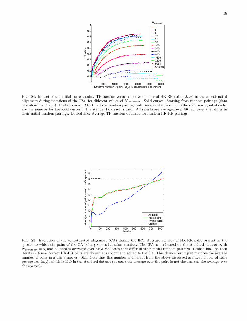
FIG. S4. Impact of the initial correct pairs. TP fraction versus effective number of HK-RR pairs (Meff) in the concatenatedalignment during iterations of the IPA, for different values of Nincrement. Solid curves: Starting from random pairings (dataalso shown in Fig. 3). Dashed curves: Starting from random pairings with no initial correct pair (the color and symbol codesare the same as for the solid curves). The standard dataset is used. All results are averaged over 50 replicates that differ intheir initial random pairings. Dotted line: Average TP fraction obtained for random HK-RR pairings.

FIG. S5. Evolution of the concatenated alignment (CA) during the IPA. Average number of HK-RR pairs present in thespecies to which the pairs of the CA belong versus iteration number. The IPA is performed on the standard dataset, withNincrement = 6, and all data is averaged over 5193 replicates that differ in their initial random pairings. Dashed line: At eachiteration, 6 new correct HK-RR pairs are chosen at random and added to the CA. This chance result just matches the averagenumber of pairs in a pair’s species: 16.1. Note that this number is different from the above-discussed average number of pairsper species 〈mp〉, which is 11.0 in the standard dataset (because the average over the pairs is not the same as the average overthe species).

19

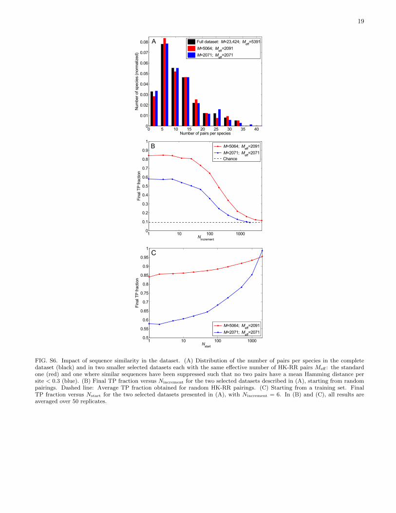
FIG. S6. Impact of sequence similarity in the dataset. (A) Distribution of the number of pairs per species in the completedataset (black) and in two smaller selected datasets each with the same effective number of HK-RR pairs Meff : the standardone (red) and one where similar sequences have been suppressed such that no two pairs have a mean Hamming distance persite < 0.3 (blue). (B) Final TP fraction versus Nincrement for the two selected datasets described in (A), starting from randompairings. Dashed line: Average TP fraction obtained for random HK-RR pairings. (C) Starting from a training set. FinalTP fraction versus Nstart for the two selected datasets presented in (A), with Nincrement = 6. In (B) and (C), all results areaveraged over 50 replicates.

20

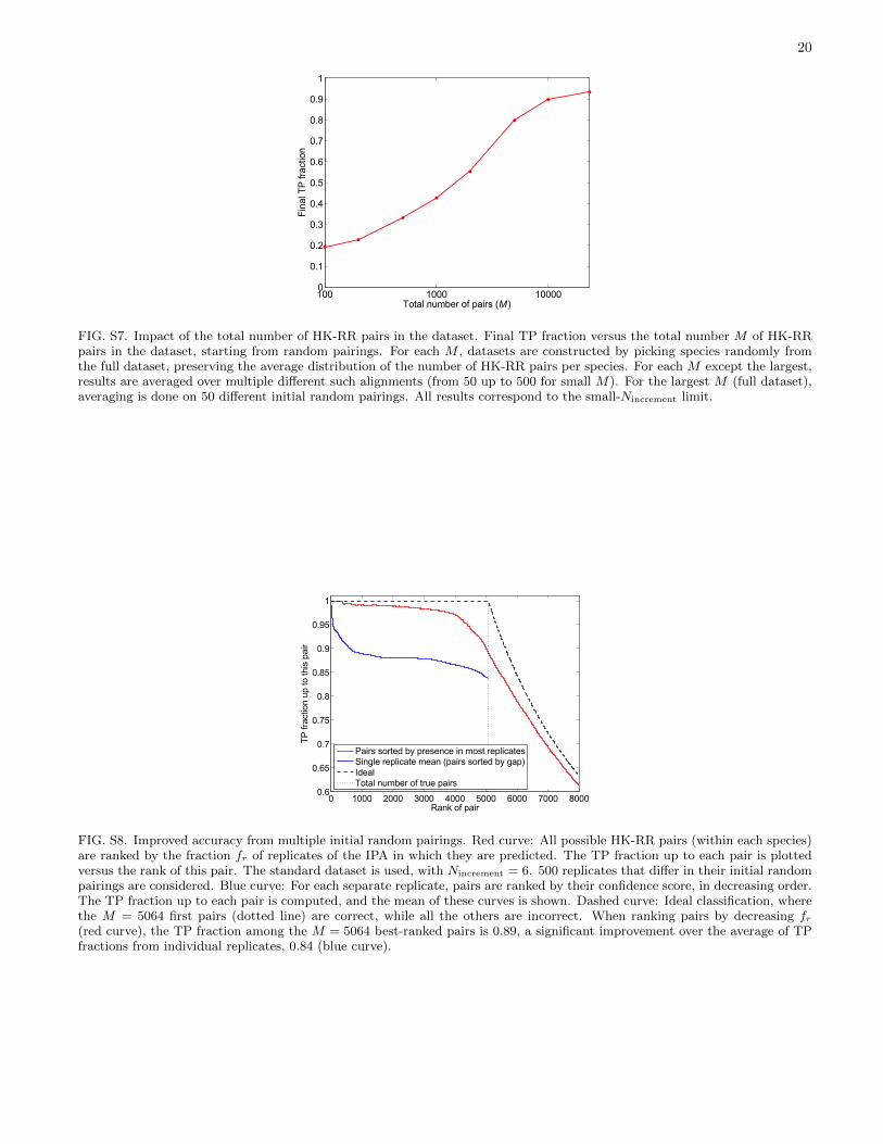
FIG. S7. Impact of the total number of HK-RR pairs in the dataset. Final TP fraction versus the total number M of HK-RRpairs in the dataset, starting from random pairings. For each M , datasets are constructed by picking species randomly fromthe full dataset, preserving the average distribution of the number of HK-RR pairs per species. For each M except the largest,results are averaged over multiple different such alignments (from 50 up to 500 for small M). For the largest M (full dataset),averaging is done on 50 different initial random pairings. All results correspond to the small-Nincrement limit.

FIG. S8. Improved accuracy from multiple initial random pairings. Red curve: All possible HK-RR pairs (within each species)are ranked by the fraction fr of replicates of the IPA in which they are predicted. The TP fraction up to each pair is plottedversus the rank of this pair. The standard dataset is used, with Nincrement = 6. 500 replicates that differ in their initial randompairings are considered. Blue curve: For each separate replicate, pairs are ranked by their confidence score, in decreasing order.The TP fraction up to each pair is computed, and the mean of these curves is shown. Dashed curve: Ideal classification, wherethe M = 5064 first pairs (dotted line) are correct, while all the others are incorrect. When ranking pairs by decreasing fr(red curve), the TP fraction among the M = 5064 best-ranked pairs is 0.89, a significant improvement over the average of TPfractions from individual replicates, 0.84 (blue curve).

21

FIG. S9. Rebootstrapping: exploiting the high TP fraction of the HK-RR pairs predicted to be correct in most replicates ofthe IPA, which differ in their initial random pairings. (A) Rebootstrapping on the standard dataset (M = 5064 HK-RR pairs).The final TP fraction is plotted versus rebootstrapping step number. Step 0 corresponds to the standard procedure describedin the main text (IPA starting from random pairings, see Fig. 6). 500 replicates are computed. We then take as a trainingset 1000 HK-RR pairs chosen randomly among those predicted to be correct in more than 50% of replicates. These pairs arechosen with probability equal to the fraction of replicates in which they are predicted to be true. The IPA is then performedagain starting from such training sets. The process is then iterated. Here, 50 replicates were computed for steps 1, 2, and 3.The average final TP fraction is plotted (blue curve), as well as the TP fraction for the best M = 5064 pairs ranked by thefraction of replicates in which they are predicted to be true (red curve, see Fig. 6). Here, Nincrement = 6. (B) Rebootstrappingon a smaller dataset with M = 502 HK-RR pairs from 40 species (mean number of pairs per species 〈mp〉 = 12.6). The processis the same as in (A), but here, at each rebootstrapping step, we take as a training set 200 HK-RR pairs chosen randomlyamong those predicted to be true in more than 25% of replicates at the previous step, and Nincrement = 1.

22

FIG. S10. Distribution of the fraction of replicates fr of the IPA in which each possible within-species HK-RR pair is predictedas a pair. (A) Red curve: Distribution of fr obtained by applying the IPA to the standard dataset (same data as in Fig. S8).Blue curve: Same dataset, but with each column of the alignment randomly scrambled. (B) HK-RR dataset with no correctpairs; a dataset of the same size as the standard one (M = 5062 in practice) that does not include any true HK-RR pairs wasconstructed. Red curve: Distribution of fr obtained by applying the IPA to this dataset with no correct pairs. Blue curve:Same alignment, but with each column randomly scrambled. For each curve, 500 IPA replicates that differ in their initialrandom pairings were used, with Nincrement = 6. All data is binned into 50 equally-spaced bins between fr = 0 and fr = 1.

23

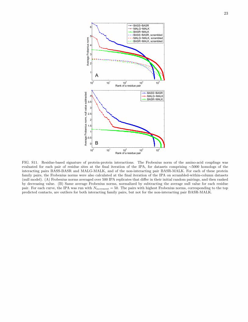
FIG. S11. Residue-based signature of protein-protein interactions. The Frobenius norm of the amino-acid couplings wasevaluated for each pair of residue sites at the final iteration of the IPA, for datasets comprising ∼5000 homologs of theinteracting pairs BASS-BASR and MALG-MALK, and of the non-interacting pair BASR-MALK. For each of these proteinfamily pairs, the Frobenius norms were also calculated at the final iteration of the IPA on scrambled-within-column datasets(null model). (A) Frobenius norms averaged over 500 IPA replicates that differ in their initial random pairings, and then rankedby decreasing value. (B) Same average Frobenius norms, normalized by subtracting the average null value for each residuepair. For each curve, the IPA was run with Nincrement = 50. The pairs with highest Frobenius norms, corresponding to the toppredicted contacts, are outliers for both interacting family pairs, but not for the non-interacting pair BASR-MALK.

24

FIG. S12. Scoring by gap. (A) Determination of the confidence score of each assigned HK-RR pair in a given iteration of theIPA. In this schematic, we consider a species with three HKs and RRs. In the energy spectra showing the interaction energiesfor each RR with all three HKs, each color represents a given HK (red: HK 1, partner of RR 1; blue: 2; green: 3). Assignment1: The pair with the lowest interaction energy (HK 2 - RR 2, boxed) is selected. The energy gap ∆ERR is shown. Here nRR = 0since no HK has been removed from consideration yet. Assignment 2: The HK and RR previously paired are removed fromfurther consideration (dashed energy levels). The next pair with the lowest energy (HK 1 - RR 3, boxed) is chosen amongthe remaining ones. Here nRR = 1 since HK 2, which was paired previously, had a lower interaction energy with RR 3 thanHK 1. Using the ad hoc confidence score ∆ERR/(nRR + 1), this (incorrect) pair is penalized with respect to the (correct) onemade in the first assignment, even though their energy gaps are similar. Assignment 3: Only one possible pair remains. It ismade, and its confidence score is taken to be equal to the lowest previously calculated confidence score for that species (thesecond one here). At each HK-RR pair assignment, symmetric confidence scores ∆EHK/(nHK + 1) are also calculated from theenergy spectra showing the interaction energies for each HK with all three RRs. The final confidence score of a pair, denotedby ∆E/(n+ 1), is the smallest of these two scores, i.e. min{∆ERR/(nRR + 1), ∆EHK/(nHK + 1)}. (B) More generally, in everyiteration of the IPA, each predicted HK-RR pair can be scored by ∆E/(n+ 1)α, where α is a parameter. Red curve: Averagefinal TP fraction obtained versus α; error bars: 95% confidence intervals around the mean. The IPA was performed on thestandard dataset, with Nincrement = 6. Results are averaged over 200 replicates that differ in their initial random pairings forall α except α = 1, for which 500 replicates were computed. As we found the highest TP fraction for α = 1, all the resultselsewhere in the paper were obtained using α = 1.

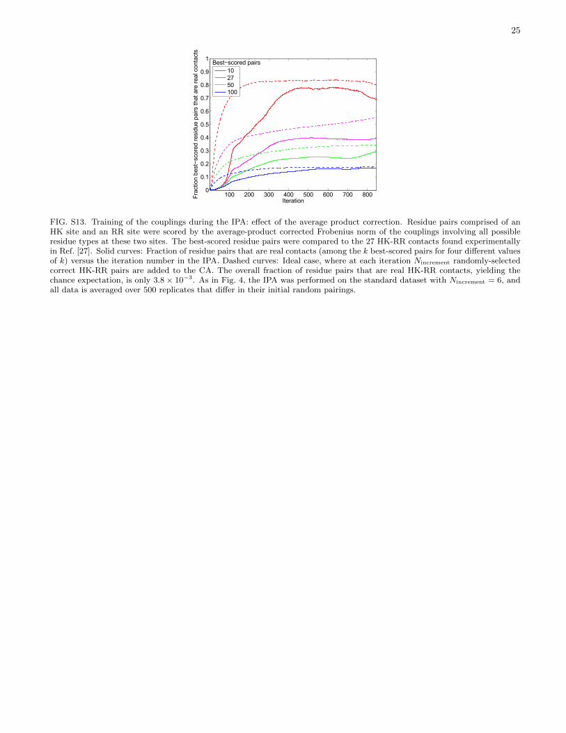
25

FIG. S13. Training of the couplings during the IPA: effect of the average product correction. Residue pairs comprised of anHK site and an RR site were scored by the average-product corrected Frobenius norm of the couplings involving all possibleresidue types at these two sites. The best-scored residue pairs were compared to the 27 HK-RR contacts found experimentallyin Ref. [27]. Solid curves: Fraction of residue pairs that are real contacts (among the k best-scored pairs for four different valuesof k) versus the iteration number in the IPA. Dashed curves: Ideal case, where at each iteration Nincrement randomly-selectedcorrect HK-RR pairs are added to the CA. The overall fraction of residue pairs that are real HK-RR contacts, yielding thechance expectation, is only 3.8× 10−3. As in Fig. 4, the IPA was performed on the standard dataset with Nincrement = 6, andall data is averaged over 500 replicates that differ in their initial random pairings.