INFINITE LATENT HARMONIC ALLOCATION: A NONPARAMETRICBAYESIAN APPROACH TO MULTIPITCH ANALYSIS

Kazuyoshi Yoshii Masataka GotoNational Institute of Advanced Industrial Science and Technology (AIST), Japan

{k.yoshii, m.goto}@aist.go.jp

ABSTRACTThis paper presents a statistical method called Infinite La-tent Harmonic Allocation (iLHA) for detecting multiplefundamental frequencies in polyphonic audio signals. Con-ventional methods face a crucial problem known as modelselection because they assume that the observed spectra aresuperpositions of a certain fixed number of bases (soundsources and/or finer parts). iLHA avoids this problem byassuming that the observed spectra are superpositions ofa stochastically-distributed unbounded (theoretically infi-nite) number of bases. Such uncertainty can be treated in aprincipled way by leveraging the state-of-the-art paradigmof machine-learning called Bayesian nonparametrics. Torepresent a set of time-sliced spectral strips, we formulatednested infinite Gaussian mixture models (GMMs) basedon hierarchical and generalized Dirichlet processes. Eachstrip is allowed to contain an unbounded number of soundsources (GMMs), each of which is allowed to contain anunbounded number of harmonic partials (Gaussians). Totrain the nested infinite GMMs efficiently, we used a mod-ern inference technique called collapsed variational Bayes(CVB). Our experiments using audio recordings of real pi-ano and guitar performances showed that fully automatediLHA based on noninformative priors performed as well asoptimally tuned conventional methods.

1. INTRODUCTION

Multipitch analysis of polyphonic audio signals [1–11] isone of the most important issues because it is the basisof many applications such as music transcription, chordrecognition, and musical instrument recognition. We focuson principled methods based on machine learning, whichhave recently yielded promising results. Some researchers,for example, have proposed generative probabilistic mod-els that explain how multiple spectral/signal bases (compo-sitional units) are mixed to form polyphonic music [3–6].The model parameters can be trained by means of statisti-cal inference. Others have used nonnegative matrix factor-ization (NMF) to decompose polyphonic spectra into indi-vidual spectral bases [7–11]. NMF can be interpreted fromthe viewpoint of statistical inference [10–12].

Permission to make digital or hard copies of all or part of this work for

personal or classroom use is granted without fee provided that copies are

not made or distributed for profit or commercial advantage and that copies

bear this notice and the full citation on the first page.c© 2010 International Society for Music Information Retrieval.

Model #2

Unified

Model

Select an optimal model

Carefully tune prior distributions

Assume the number of spectral bases

Output:

Fundamental frequencies (F0s)

Input:

Polyphonic

audio signals

Conventional methods

…Model #1

Assume the number of harmonic partials

Our method (iLHA)

No prior tuning

Require

No assumptions

Figure 1. Methodological advantage of our method.

A crucial problem in these methods, known as modelselection, is that they perform best only if an appropriatemodel complexity (the number of bases) is specified in ad-vance. One might think that the optimal number of basesmust be equal to the number of sound sources, but it is notclear how many bases are most suited to represent a singlesource if the spectral shape varies through time. Althoughuncertainty is inherent in model selection, conventionalmethods assume that a certain complexity exists uniquelyas an oracle. As shown in Figure 1, they require possiblemodels to be examined separately and exhaustively and theoptimal model selected in retrospect. Such a determinis-tic framework is not easy-to-use in practice although opti-mally tuned methods can achieve good performance.

To avoid model selection, we propose a novel statisticalmethod called Infinite Latent Harmonic Allocation (iLHA)based on a modern paradigm of machine learning calledBayesian nonparametrics. Note that the term “nonpara-metric” means that we do not have to fix model complexityuniquely. We assume that an unbounded but finite numberof bases stochastically appears in a limited amount of avail-able data although an infinite number of bases theoreticallyexists in the universe. Uncertainty in model selection canbe treated reasonably in a probabilistic framework.

iLHA can be derived by taking the infinite limit of con-ventional finite models [3, 4]. Conventionally, each spec-tral basis is often parameterized by means of a Gaussianmixture model (GMM) in which a fixed number of Gaus-sians corresponds to the spectral peaks of harmonic par-tials, and a time-sliced polyphonic spectral strip is modeledby mixing a fixed number of GMMs. Here, we considerboth the number of bases and the number of partials to ap-proach infinity, where most are regarded as unnecessaryand automatically removed through statistical inference.

A fundamental and practically-important advantage ofiLHA is that precise prior knowledge is not required. Con-ventional methods [3–5] heavily rely on prior distributionsregarding the relative strengths of harmonic partials, which

309

11th International Society for Music Information Retrieval Conference (ISMIR 2010)

have too much impact on performance, and forced us totune priors and their weighting factors by hand accordingto the properties of target sound sources. iLHA, in contrast,can be fully automated by layering noninformative hyper-priors on influential priors in a hierarchical Bayesian man-ner. This is consistent with the fact that humans can adap-tively distinguish individual notes of various instruments.One of major contributions of this study is to embody thefundamental Bayesian principle “Let the data speak for it-self” in the context of multipitch analysis.

The rest of this paper is organized as follows: Section 2describes statistical interpretation of polyphonic spectra.Section 3 discusses related work. Sections 4 and 5 explainfinite models (LHA) and infinite models (iLHA). Section 6reports our experiments. Section 7 concludes this paper.

2. STATISTICAL INTERPRETATION

We interpret polyphonic spectra as histograms of observedfrequencies that independently occur. This interpretationbasically follows conventional studies [3–5].

2.1 Assumptions

Suppose given polyphonic audio signals are generated fromK bases, each of which consists of M harmonic partialslocated on a linear frequency scale at integral multiples ofthe fundamental frequency (F0). Note that each basis canbe associated with multiple sounds of different temporalpositions if these sounds are derived from the same pitchof the same instrument. We transform the audio signalsinto wavelet spectra. Let D be the number of frames. If aspectral strip at frame d (1 ≤ d ≤ D) has amplitude a atfrequency f , we assume that frequency f was observed a

times in frame d. Assuming that amplitudes are additive,we can consider each observed frequency to be generatedfrom one of M partials in one of K bases.

These notations are for the finite case. In Bayesian non-parametrics, we take the limit as K and M go to infinity.

2.2 Observed and Latent Variables

Let the total observed variables over all D frames be rep-resented by X = {X1, · · · ,XD}, where Xd is a set ofobserved frequencies Xd = {xd1, · · · ,xdNd

} in frame d.Nd is the number of frequency observations. That is, Nd isequal to the sum of spectral amplitudes over all frequencybins in frame d. xdn (1 ≤ n ≤ Nd) is an one-dimensionalvector that represents an observed frequency.

Let the total latent variables corresponding to X be sim-ilarly represented by Z = {Z1, · · · ,ZD}, where Zd =

{zd1, · · · ,zdNd}. zdn is a KM-dimensional vector in which

only one entry, zdnkm, takes a value of 1 and the others takevalues of 0 when frequency xdn is generated from partialm (1 ≤ m ≤ M) of basis k (1 ≤ k ≤ K).

3. COMPARISON WITH RELATED WORK

The properties of iLHA are intermediate between those oftwo successful approaches–statistical inference and NMF–which are discussed here for comparison and to clarify thepositioning of our approach.

Frequency

(Cent)

Density

kµ

2o

k+µ

mko+μL L

1−Λ

k 1kτ

2kτ km

τ

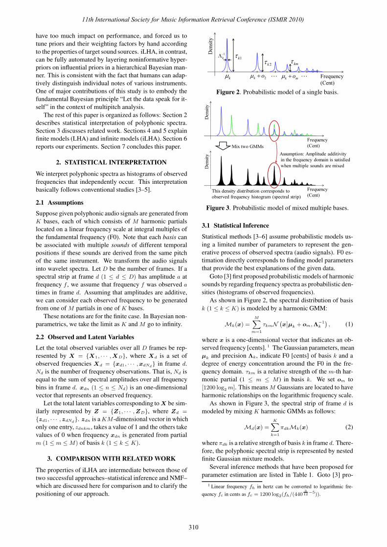
Figure 2. Probabilistic model of a single basis.

Frequency

(Cent)

Density

Frequency

(Cent)

Density

Assumption: Amplitude additivity

in the frequency domain is satisfied

when multiple sounds are mixed

Mix two GMMs

This density distribution corresponds to

observed frequency histogram (spectral strip)

Figure 3. Probabilistic model of mixed multiple bases.

3.1 Statistical Inference

Statistical methods [3–6] assume probabilistic models us-ing a limited number of parameters to represent the gen-erative process of observed spectra (audio signals). F0 es-timation directly corresponds to finding model parametersthat provide the best explanations of the given data.

Goto [3] first proposed probabilistic models of harmonicsounds by regarding frequency spectra as probabilistic den-sities (histograms of observed frequencies).

As shown in Figure 2, the spectral distribution of basisk (1 ≤ k ≤ K) is modeled by a harmonic GMM:

Mk(x) =

M∑

m=1

τkmN (

x∣

∣μk + om,Λ−1k

)

, (1)

where x is a one-dimensional vector that indicates an ob-served frequency [cents]. 1 The Gaussian parameters, meanμk and precision Λk, indicate F0 [cents] of basis k and adegree of energy concentration around the F0 in the fre-quency domain. τkm is a relative strength of the m-th har-monic partial (1 ≤ m ≤ M) in basis k. We set om to[1200 log2 m]. This means M Gaussians are located to haveharmonic relationships on the logarithmic frequency scale.

As shown in Figure 3, the spectral strip of frame d ismodeled by mixing K harmonic GMMs as follows:

Md(x) =K∑

k=1

πdkMk(x) (2)

where πdk is a relative strength of basis k in frame d. There-fore, the polyphonic spectral strip is represented by nestedfinite Gaussian mixture models.

Several inference methods that have been proposed forparameter estimation are listed in Table 1. Goto [3] pro-

1 Linear frequency fh in hertz can be converted to logarithmic fre-quency fc in cents as fc = 1200 log2(fh/(440

312

−5)).

310

11th International Society for Music Information Retrieval Conference (ISMIR 2010)

#(bases) #(partials) Temporal modelingPreFEst [3] Fixed Fixed None

HC [4] Inferred Fixed NoneHTC [5] Fixed Fixed Continuity treatedNMF [7] Fixed Not used Exchangeable

iLHA Infinite Infinite Exchangeable

Table 1. Comparison of multipitch analysis methods.

posed a method called PreFEst that estimates only relativestrengths τ and π while μ and Λ are fixed by allocatingmany GMMs to cover the entire frequency range as F0 can-didates. Kameoka et al. [4] then proposed harmonic clus-tering (HC), which estimates all the parameters and selectsthe optimal number of bases by using the Akaike informa-tion criterion (AIC). Although these methods yielded thepromising results, they analyze the spectral strips of differ-ent frames independently. Thus, Kameoka et al. [5] pro-posed harmonic-temporal-structured clustering (HTC) thatcaptures temporal continuity of spectral bases. Note thatall these methods are based on maximum-likelihood andmaximum-a-posteriori training of the parameters by intro-ducing prior distributions of relative strengths τ , whichhave a strong impact on the accuracy of F0 estimation.

Our method called iLHA is based on hierarchical non-parametric Bayesian modeling that requires no prior tuningand avoids specifying K and M in advance. More specif-ically, the limit of the conventional nested finite GMMs isconsidered as K and M diverge to infinity.

3.2 Nonnegative Matrix FactorizationNMF-based methods [7–12] factorize observed frequencyspectra into the product of spectral bases and time-varyingenvelopes under the nonnegativity constraint. K bases areestimated by sweeping all frames of the given spectra. Al-though several methods [10, 12] take temporal continuityinto account, standard methods are based on temporal ex-changeability. In other words, exchange of arbitrary framesdoes not affect the factorized results. Although such tem-poral modeling is not sufficient, it is known to work wellin practice. Therefore, iLHA adopted the exchangeability.

4. LATENT HARMONIC ALLOCATION

This section explains LHA, the finite version of iLHA, as apreliminary step to deriving iLHA. We formulate the con-ventional nested finite GMMs in a Bayesian manner.

4.1 Model FormulationFigure 4 illustrates a graphical representation of the LHAmodel. The full joint distribution is given by

p(X,Z,π, τ ,μ,Λ)

= p(X|Z,μ,Λ)p(Z|π, τ )p(π)p(τ)p(μ,Λ) (3)

where the first two terms on the right-hand side are likeli-hood functions and the other three terms are prior distribu-tions. The likelihood functions are defined as

p(X|Z,μ,Λ) =∏

dnkm

N (

xdn

∣

∣μk + om,Λ−1k

)zdnkm (4)

p(Z|π, τ ) =∏

dnkm

(πdkτkm)zdnkm (5)

dnz

dnx

�D

kmτ

kµ

00,bm

kΛ

00,cW

βK

dπα

ν

υM

Figure 4. A graphical representation of LHA.

Then, we introduce conjugate priors as follows:

p(π) =

D∏

d=1

Dir(πd|αν) ∝D∏

d=1

K∏

k=1

πανk−1dk (6)

p(τ ) =K∏

k=1

Dir(τk|βυ) ∝K∏

k=1

M∏

m=1

τβυm−1km (7)

p(μ,Λ) =

K∏

k=1

N (

μk

∣

∣m0, (b0Λk)−1

)W (

Λk

∣

∣W 0, c0)

(8)

where p(π) and p(τ) are products of Dirichlet distributionsand p(μ,Λ) is a product of Gaussian-Wishart distributions.αν and βυ are hyperparameters and α and β are calledconcentration parameters when ν and υ sum to unity. m0,b0, W 0, and c0 are also hyperparameters; W 0 is a scalematrix and c0 is a degree of freedom.

4.2 Variational Bayesian InferenceThe objective of Bayesian inference is to compute a trueposterior distribution of all variables: p(Z,π, τ ,μ,Λ|X).Because analytical calculation of the posterior distributionis intractable, we instead approximate it by using iterativeinference techniques such as variational Bayes (VB) andMarkov chain Monte Carlo (MCMC). Although MCMCis considered to be more accurate in general, we use VBbecause it converges much faster.

In the VB framework, we introduce a variational pos-terior distribution q(Z,π, τ ,μ,Λ) and make it close to thetrue posterior p(Z,π, τ ,μ,Λ|X) iteratively. Here, we as-sume that the variational distribution can be factorized as

q(Z,π, τ ,μ,Λ) = q(Z)q(π, τ ,μ,Λ) (9)

To optimize q(Z,π, τ ,μ,Λ), we use a variational ver-sion of the Expectation-Maximization (EM) algorithm [13].We iterate VB-E and VB-M steps until a variational lowerbound of evidence p(X) converges as follows:

q∗(Z) ∝ exp(

Eπ,τ ,μ,Λ [log p(X,Z,π, τ ,μ,Λ)])

(10)

q∗(π, τ ,μ,Λ) ∝ exp (EZ [log p(X,Z,π, τ ,μ,Λ)]) (11)

4.3 Updating FormulaWe derive the formulas for updating variational posteriordistributions according to Eqns. (10) and (11).

4.3.1 VB-E Step

An optimal variational posterior distribution of latent vari-ables Z can be computed as follows:

log q∗(Z) = Eπ,τ ,μ,Λ [log p(X,Z,π, τ ,μ,Λ)] + const.

= Eμ,Λ [log p(X|Z,μ,Λ)] + Eπ,τ [log p(Z|π, τ )] + const.

=∑

dnkm

zdnkm log ρdnkm + const. (12)

311

11th International Society for Music Information Retrieval Conference (ISMIR 2010)

1

~

ν1

~1 ν−

2

~

ν2

~1 ν−

3

~

ν3

~1 ν−

1ν

2ν

3ν

L

:

:

:

Recursively break

the stick of length 1

Figure 5. Stick-breaking construction of Dirichlet process.

where ρdnkm is defined as

log ρdnkm = Eπd [log πdk] + Eτk [log τkm]

+Eμk,Λk

[

logN (

xdn

∣

∣μk + om,Λ−1k

)]

(13)

q∗(Z) is obtained as multinomial distributions given by

q∗(Z) =∏

dnkm

γzdnkmdnkm (14)

where γdnkm is given by γdnkm = ρdnkm∑km ρdnkm

and is calleda responsibility that indicates how likely it is that observedfrequency xdn is generated from harmonic partial m of ba-sis k. Here, let ndkm be an observation count that indicateshow many frequencies were generated from harmonic par-tial m of basis k in frame d. ndkm and its expected valuecan be calculated as follows:

ndkm =∑

n

zdnkm E[ndkm] =∑

n

γdnkm (15)

For convenience in executing the VB-M step, we com-pute several sufficient statistics as follows:

Sk[1]≡∑

dnm

γdnkm Sk[x] ≡∑

dnm

γdnkmxdnm (16)

Sk[xxT ]≡

∑

dnm

γdnkmxdnmxTdnm (17)

where xdnm is defined as xdnm = xdn − om.

4.3.2 VB-M Step

Consequently, an optimal variational posterior distributionof parameters π, τ ,μ,Λ is shown to be given by

q∗(π, τ ,μ,Λ) =D∏

d=1

q∗(πd)K∏

k=1

q∗(τk)K∏

k=1

q∗(μk,Λk) (18)

Since we use conjugate priors, each posterior has the sameform of the corresponding prior as follows:

q∗(πd) = Dir(πd|αd) (19)

q∗(τk) = Dir(τk|βk) (20)

q∗(μk,Λk) =N (

μk

∣

∣mk, (bkΛk)−1)W (

Λk

∣

∣W k, ck)

(21)

where the variational parameters are given by

αdk = ανk + E[ndk·] βkm = βυm + E[n·km] (22)

bk = b0 + Sk[1] ck = c0 + Sk[1] (23)

mk =b0m0 + Sk[x]

b0 + Sk[1]=

b0m0 + Sk[x]

bk(24)

W−1k =W−1

0 + b0m0mT0 + Sk[xx

T ]− bkmkmTk (25)

Here dot (·) denotes the sum over that index.

5. INFINITE LATENT HARMONIC ALLOCATION

This section derives hierarchical nonparametric Bayesianmodels, i.e., nested infinite GMMs for polyphonic spectra.

5.1 Model Formulation

First we let K approach infinity, where the infinite numberof harmonic GMMs is assumed to exist in the universe.More specifically, the dimensionality of the Dirichlet dis-tributions in Eqn. (6) is considered to be infinite. At eachframe d, πd is an infinite vector of normalized probabili-ties (mixing weights) drawn from the infinite-dimensionalDirichlet prior. Such stochastic process is called a Dirichletprocess (DP). Every time frequency xdn is generated, oneof the infinite number of harmonic GMMs is drawn accord-ing to πd. Note that most entries of πd take extremely tinyvalues because all entries sum to unity. If we can observethe infinite number of frequencies (Nd → ∞), the infinitenumber of harmonic GMMs can be drawn. However, Nd

is finite in practice. Therefore, only the finite number ofharmonic GMMs, K+ � ∞, is drawn at frame d. Here,a problem is that harmonic GMMs that are actually drawnat frame d are completely disjointed from those drawn atanother frame d′. This is not a reasonable situation.

To solve this problem, we use the hierarchical DirichletProcess (HDP) [14]. More specifically, we assume thatinfinite-dimensional hyperparameter ν in Eqn. (6), whichis shared among all D frames, is a draw from a top-levelDP. A generative interpretation is that after an unboundednumber of harmonic GMMs is initially drawn from the top-level DP, an unbounded subset is further drawn accordingto the local DP at each frame. This effectively ties frame d

to another frame d′. As shown in Figure 5, ν is known tofollow the stick-breaking construction [14] as follows:

νk = ν̃k

k−1∏

k′=1

(1− ν̃k′) ν̃k ∼ Beta(1, γ) (26)

where γ is a concentration parameter of the top-level DP.Therefore ν can be converted into ν̃.

Now we let M approach infinity, where each harmonicGMM consists of the infinite number of harmonic partials.To put effective priors on τ , we use generalized DPs calledBeta two-parameter processes as follows:

τkm = τ̃km

m−1∏

m′=1

(1− τ̃km′) τ̃km ∼ Beta(βλ1, βλ2) (27)

where β is a positive scalar and λ1 + λ2 = 1.Because α, β, γ and λ are influential hyperparameters,

we put Gamma and Beta hyperpriors on them as follows:

p(α) = Gam(α|aα, bα) p(γ) = Gam(γ|aγ , bγ) (28)

p(β) = Gam(β|aβ, bβ) p(λ) = Beta(λ|u1, u2) (29)

where a{α,β,γ} and b{α,β,γ} are shape and rate parameters.Figure 6 shows a graphical representation of the iLHA

model. The full joint distribution is given by

p(X,Z,π, τ̃ ,μ,Λ, α, β, γ,λ, ν̃) = p(X|Z,μ,Λ)p(μ,Λ)

p(Z|π, τ̃ )p(π|α, ν̃)p(τ̃ |β,λ)p(α)p(β)p(γ)p(λ)p(ν̃|γ) (30)

where p(Z|π, τ̃ ) is obtained by plugging Eqn. (27) intoEqn. (5) and p(π|α, ν) is the same as Eqn. (6). p(ν̃|γ) andp(τ̃ |β,λ) are defined according to Eqns. (26) and (27) as

p(ν̃|γ) =∏

k

Beta(τ̃k|1, γ) p(τ̃ |β,λ) =∏

km

Beta(τ̃km|βλ)(31)

312

11th International Society for Music Information Retrieval Conference (ISMIR 2010)

dπ

�D

kmτ~

00,bm

00,cW

K

βββ ba ,

αααba ,

γk

ν~

M

∞→M

∞→K

kµ

kΛ

γγba ,

dnz

dnx

λ u

Figure 6. A graphical representation of iLHA.

5.2 Collapsed Variational Bayesian InferenceTo train the HDP model we use a sophisticated version ofVB called collapsed variational Bayes (CVB) [15]. CVBenables more accurate posterior approximation in the spaceof latent variables where parameters are integrated out.

Figure 7 shows a collapsed iLHA model. By integratingout π, τ̃ ,μ,Λ, we obtain the marginal distribution given by

p(X,Z, α, β, γ,λ, ν̃)

= p(X|Z)p(Z|α, β,λ, ν̃)p(α)p(β)p(γ)p(λ)p(ν̃|γ) (32)

where the first two terms are calculated as follows:

p(X|Z) = (2π)−n···2

∏

k

(

b0bzk

) 12 B(W 0, c0)

B(W zk, czk)(33)

p(Z|α, β,λ, ν̃) =∏

d

Γ(α)

Γ(α+ nd··)

∏

k

Γ(ανk + ndk·)Γ(ανk)

∏

km

Γ(β)Γ(βλ1 + n·km)Γ(βλ2 + n·k>m)

Γ(βλ1)Γ(βλ2)Γ(β + n·k≥m)(34)

where bzk,W zk, czk are obtained by substituting zdnkm forγdnkm in calculating Eqns. (23) and (25).

Because CVB cannot be applied directly to Eqn. (32),we introduce auxiliary variables by using a technique calleddata augmentation [15]. Let ηd and ξkm be Beta-distributedvariables and sdk and tkm be positive integers that satisfy1 ≤ sdk ≤ ndk·, 1 ≤ tkm1 ≤ n·km, and 1 ≤ tkm2 ≤ n·k>m.Eqn. (34) can be augmented as

p(Z,η, ξ, s, t|α, β,λ, ν̃) =∏

d

ηα−1d

(1 − ηd)nd··−1

Γ(nd··)

∏

k

[ndk·sdk

]

(ανk)sdk

∏

km

ξβ−1km

(1 − ξkm)n·k≥m−1

Γ(n·k≥m)

[n·km

tkm1

]

(βλ1)tkm1

[n·k>m

tkm2

]

(βλ2)tkm2

where [ ] denotes a Stirling number of the first kind. Theaugmented marginal distribution is given by

p(X,Z,η, ξ, s, t, α, β, γ,λ, ν̃)

= p(Z,η, ξ, s, t|α, β,λ, ν̃)p(α)p(β)p(γ)p(λ)p(ν̃|γ) (35)

In the CVB framework, we assume that the variationalposterior distribution can be factorized as follows:

q(Z,η, ξ, s, t, α, β, γ,λ, ν̃)

= q(α, β, γ,λ)q(ν̃)q(η, ξ, s, t|Z)∏

dn

q(zdn) (36)

We also use an approximation technique called varia-tional posterior truncation. More specifically, we assumeq(zdnkm) = 0 when k > K and m > M . In practice, it isenough that K and M are set to sufficiently large integers.

5.3 Updating FormulaWe descrive the formulas for updating variational posteriordistributions.

�D

K

α

γk

ν~

∞→M

∞→K

dη

ds

00,bm

00,cW

ααba ,

γγba ,

dnz

dnx

βββ ba , u

M

kmξ

kmt

λ

Figure 7. A collapsed model with auxiliary variables.

5.3.1 CVB-E Step

A variational probability of zdnkm = 1 is given by

log q∗(zdnkm = 1) = Ez¬dn

[

log(

G[ανk] + n¬dndk·

)]

+ Ez¬dn

[

log

(

G[βλ1] + n¬dn·km

E[β] + n¬dn·k≥m

m−1∏

m′=1

G[βλ2] + n¬dn·k>m′

E[β] + n¬dn·k≥m′

)]

+ Ez¬dn

[

log S(xdnm|m¬dnzk ,L¬dn

zk , c¬dnzk )

]

+ const. (37)

where subscript ¬dn denotes a set of indices without d andn, G[x] denotes the geometric average exp(E[log x]), andS is the Student-t distribution. L¬dn

zk is given by L¬dnzk =

b¬dnzk

1+b¬dnzk

c¬dnzk W ¬dn

zk , where m¬dnzk , b¬dn

zk ,W¬dnzk , c¬dn

zk are ob-tained by substituting zdnkm for γdnkm required by Eqns.(23), (24), and (25) and calculating sum without zdn. Eachterm of Eqn. (37) can be calculated efficiently [15, 16].

5.3.2 CVB-M Step

First, α, β and γ are Gamma distributed as follows:

q(α)∝ αaα+E[s··]−1e−α(bα−∑d E[log ηd]) (38)

q(β)∝ βaβ+E[t···]−1e−β(bβ−∑km E[log ξkm]) (39)

q(γ)∝ γaγ+K−1e−γ(bγ−∑k E[log(1−ν̃k)]) (40)

Then, λ and τ̃ are Beta distributed as follows:

q∗(λ)∝ λu1+E[t··1]−11 λ

u2+E[t··2]−12 (41)

q∗(ν̃k)∝ ν̃1+E[s·k]−1k (1− ν̃k)

E[γ]+E[s·>k]−1 (42)

Finally, the variational posteriors of η, ξ, s, t are given by

q∗(ηd)∝ ηE[α]−1d (1− ηd)

nd··−1 (43)

q∗(ξkm|Z)∝ ξE[β]−1km (1− ξkm)n·k≥m−1 (44)

q∗(sdk = s|Z)∝[

ndk·s

]

G[ανk]s (45)

q∗(tkm1 = t|Z)∝[

n·km

t

]

G[βλ1]t (46)

q∗(tkm2 = t|Z)∝[

n·k>m

t

]

G[βλ2]t (47)

To calculate E[sdk] (average sdk over Z), we exactly treatthe case ndk· = 0 and apply second-order approximationwhen ndk· > 0 (see details in [15]). E[log ξkm], E[tkm1],and E[tkm2] can be calculated in the same way.

To estimate F0s, we need explicitly compute the varia-tional posteriors of the integrated-out parameters μ,Λ. Todo this, we execute the standard VB-M step once by usingthe responsibilities q(Z) obtained in the CVB-E step.

6. EVALUATION

This section reports our comparative experiments evaluat-ing the performance of iLHA.

313

11th International Society for Music Information Retrieval Conference (ISMIR 2010)

Piece number Optimally tuned Fully automatedRWC-MDB- PreFEst [3] HTC [5] LHA iLHAJ-2001 No.1 75.8 79.0 70.7 82.2J-2001 No.2 78.5 78.0 69.1 77.9J-2001 No.6 70.4 78.3 49.8 71.2J-2001 No.7 83.0 86.0 70.2 85.5J-2001 No.8 85.7 84.4 55.9 84.6J-2001 No.9 85.9 89.5 68.9 84.7

C-2001 No.30 76.0 83.6 81.4 81.6C-2001 No.35 72.8 76.0 58.9 79.6

Total 79.4 82.0 65.8 81.7

Table 2. Frame-level F-measures of F0 detection.

6.1 Experimental ConditionsWe evaluated LHA and iLHA on the same test set used in[5], which consisted of nine pieces of piano and guitar soloperformances excerpted from the RWC music database [17].The first 23 [s] of each piece were used for evaluation. Thespectral analysis was conducted by the wavelet transformusing Gabor wavelets with a time resolution of 16 [ms].The values and temporal positions of actual F0s were pre-pared by hand as ground truth. We evaluated performancein terms of frame-level F-measures. The priors and hyper-priors of LHA and iLHA were set to noninformative uni-form distributions. K and M were set to sufficiently largenumbers, 60 and 15. iLHA is not sensitive to these values.No other tuning was required. To output F0s at each frame,we extracted bases whose expected weights π were over athreshold, which was optimized as in [5].

For comparison, we referred to the experimental resultsof PreFEst and HTC reported in [5]. Although the ground-truth data was slightly different from ours, it would be suf-ficient for roughly evaluating performance comparatively.The number of bases, priors, and weighting factors werecarefully tuned by using the ground-truth data to optimizethe results. Although this is not realistic, the upper boundsof potential performance were investigated in [5].

6.2 Experimental ResultsThe results listed in Table 2 show that the performance ofiLHA approached and sometimes surpassed that of HTC.This is consistent with the empirical findings of many stud-ies on Bayesian nonparametrics that nonparametric modelswere competitive against optimally-tuned parametric mod-els. HTC outperformed PreFEst because HTC can appro-priately deal with temporal continuity of spectral bases.This implies that incorporating temporal modeling wouldimprove the performance of iLHA.

The results of LHA were worse than those of iLHA be-cause LHA is not based on hierarchical Bayesian modelingand requires precise priors. In fact, we confirmed that theresults of PreFEst and HTC based on MAP estimation weredrastically degraded when we used noninformative priors.In contrast, iLHA stably showed the good performance.

7. CONCLUSION

This paper presented a novel statistical method for detect-ing multiple F0s in polyphonic audio signals. The methodallows polyphonic spectra to contain an unbounded num-ber of spectral bases, each of which can consist of an un-

bounded number of harmonic partials. These numbers canbe statistically inferred at the same time that F0s are esti-mated. Even in experimental evaluation using noninforma-tive priors, our automated method performed well or betterthan conventional methods manually optimized by trial anderror. To our knowledge, this is the first attempt to applyBayesian nonparametrics to multipitch analysis.

Bayesian nonparametrics is an ultimate methodologicalframework avoiding the model selection problem faced invarious areas of MIR. For example, how many sectionsshould one use for structuring a musical piece? How manygroups should one use for clustering listeners according totheir tastes or musical pieces according to their contents?We are freed from these problems by assuming that in the-ory there is an infinite number of classes behind observeddata. Unnecessary classes are automatically removed fromconsideration through statistical inference. We plan to usethis powerful framework in a wide range of applications.

Acknowledgement: This study was partially supported byJST CREST and JSPS KAKENHI 20800084.

8. REFERENCES[1] A. Klapuri. Multipitch analysis of polyphonic music and

speech signals using an auditory model. IEEE Trans. onASLP, Vol. 16, No. 2, pp. 255–266, 2008.

[2] M. Marolt. A connectionist approach to transcription of poly-phonic piano music. IEEE Trans. on Multimedia, Vol. 6,No. 3, pp. 439–449, 2004.

[3] M. Goto. A real-time music scene description system:Predominant-F0 estimation for detecting melody and basslines in real-world audio signals. Speech Communication,Vol. 43, No. 4, pp. 311–329, 2004.

[4] H. Kameoka et al. Separation of harmonic structures basedon tied Gaussian mixture model and information criterion forconcurrent sounds. ICASSP, Vol. 4, pp. 297–300, 2004.

[5] H. Kameoka et al. A multipitch analyzer based on har-monic temporal structured clustering. IEEE Trans. on ASLP,Vol. 15, No. 3, pp. 982–994, 2007.

[6] A. Cemgil et al. A generative model for music transcription.IEEE Trans. on ASLP, Vol. 14, No. 2, pp. 679–694, 2006.

[7] P. Smaragdis and J. Brown. Nonnegative matrix factorizationfor polyphonic music transcription. WASPAA, 2003.

[8] A. Cont. Realtime multiple pitch observation using sparsenon-negative constraints. ISMIR, pp. 206–211, 2006.

[9] E. Vincent et al. Adaptive harmonic spectral decompositionfor multiple pitch estimation. IEEE Trans. on ASLP, Vol. 18,No. 3, pp. 528–537, 2010.

[10] N. Bertin et al. Enforcing harmonicity and smoothness inBayesian non-negative matrix factorization applied to poly-phonic music transcription. IEEE Trans. on ASLP, Vol. 18,No. 3, pp. 538–549, 2010.

[11] P. Peeling et al. Generative spectrogram factorization mod-els for polyphonic piano transcription. IEEE Trans. on ASLP,Vol. 18, No. 3, pp. 519–527, 2010.

[12] T. Virtanen et al. Bayesian extensions to nonnegative matrixfactorisation for audio signal modelling. ICASSP, 2008.

[13] H. Attias. A variational Bayesian framework for graphicalmodels. NIPS, pp. 209–215, 2000.

[14] Y. W. Teh et al. Hierarchical Dirichlet processes. J. of Am.Stat. Assoc., Vol. 101, No. 476, pp. 1566–1581, 2006.

[15] Y. W. Teh et al. Collapsed variational inference for HDP.NIPS, Vol. 20, 2008.

[16] J. Sung et al. Latent-space variational Bayes. IEEE Trans. onPAMI, Vol. 30, No. 12, pp. 2236–2242, 2008.

[17] M. Goto et al. RWC music database: Popular, classical, andjazz music database. ISMIR, pp. 287–288, 2002.

314

11th International Society for Music Information Retrieval Conference (ISMIR 2010)