1

INFLATION AND ESCALATION BEST PRACTICES FOR COST ANALYSIS:

ANALYST HANDBOOK

OFFICE OF THE SECRETARY OF DEFENSE

COST ASSESSMENT AND PROGRAM EVALUATION, JANUARY 2017

2

About This Publication:

This study was performed in collaboration with the cost community in the Department of Defense, including the Office of the Secretary of Defense, Cost Assessment and Program Evaluation (OSD CAPE), the Assistant Secretary of the Air Force for Financial Management (SAF-FM), the Air Force Cost Analysis Agency (AFCAA), the Naval Cost Center for Analysis (NCCA), the Naval Systems Cost Engineering and Industrial Analysis Division (NAVSEA 05C), the Assistant Secretary of the Army, Financial Management (ASA-FM), and the Deputy Assistant Secretary of the Army for Cost and Economics (DASA-CE), as well as consultant support from Technomics, Inc. and the Institute for Defense Analyses (IDA).

Prepared for:

Office of the Secretary of Defense Cost Assessment and Program Evaluation January, 2017

3

Contents Preface..................................................................................................................................5 1. Introduction .................................................................................................................7

A. Background and Purpose .....................................................................................7 B. Scope ...................................................................................................................8

2. Terminology ................................................................................................................9 A. Inflation ...............................................................................................................9 B. Escalation ..........................................................................................................10 C. Real Price Change .............................................................................................11 D. Constant Year (CY) Dollars ..............................................................................12 E. Constant Price (CP) ...........................................................................................12 F. A Numerical Example .......................................................................................13

3. Framework for Analyzing Escalation ........................................................................14 A. Inflation .............................................................................................................14 B. Specific Market Prices .......................................................................................15 C. Contractor Business Effects ..............................................................................15 D. Government Effects ...........................................................................................16 E. Economy ............................................................................................................16

4. Estimating Realistic Then Year Costs .......................................................................17 A. Applying the Framework to Lower Levels of Cost Detail ................................17 B. Applying the Framework to Cost Estimating Methodologies ...........................18 C. Forward Pricing .................................................................................................19 D. Forecasting Prices Beyond the Future Year’s Defense Program ......................20

5. Normalizing for Decision Support ............................................................................23 A. Affordability Analysis .......................................................................................23 B. Comparing Alternative Purchases .....................................................................25 C. Measuring Program Performance ......................................................................27

6. Normalizing for Cost Estimation ...............................................................................30 A. Normalizing for Cost Estimating Relationships (CERs) ...................................30 B. Normalizing for Learning Curve Analyses .......................................................33

7. Selecting an Escalation Index ....................................................................................38 A. Index Attributes .................................................................................................38 B. Index Selection ..................................................................................................40

8. Index Documentation ................................................................................................43 A. Documenting Use of a Published Index ............................................................43 B. Documenting Use of a Custom Index ...............................................................44 C. Labeling Charts and Tables ...............................................................................44

9. Understanding Published DoD Indexes .....................................................................47 A. Pricing Guidance for the President’s Budget ....................................................47 B. Service-Level Indexes .......................................................................................48

4

1. Air Force Indexes ........................................................................................48 2. Army/Navy Joint Inflation Calculator (JIC) ...............................................49 3. Additional Sources ......................................................................................50

C. Overview ...........................................................................................................51 10. Escalation Resources .................................................................................................52

A. Price Indexes and Quality ..................................................................................52 B. Producer Price Indexes ......................................................................................53 C. Bureau of Economic Analysis (BEA) Deflators ...............................................54 D. Public Labor Cost Data .....................................................................................54

1. National Compensation Survey ...................................................................55 2. Occupational Employment Statistics Survey ..............................................56 3. Current Population Survey ..........................................................................56

E. Contractor Forward Pricing Rate (FPR) Data ...................................................56 F. Forecasting Resources .......................................................................................57

11. Appendices ................................................................................................................58 A. Expanded Glossary ............................................................................................58 B. Mathematical Glossary ......................................................................................58 C. Intermediate Escalation Application in CER Development ..............................64 D. Normalizing for Learning Curves: Estimating Using Actuals ..........................67 E. Understanding Legislation, OMB and Comptroller Guidance ..........................70 F. Selecting a Raw or Weighted Index ..................................................................76 G. Developing a Raw Index ...................................................................................77 H. Developing a Weighted Index ...........................................................................79 I. Categorizing Joint Inflation Calculator (JIC) Indexes ......................................83 J. Selected Defense-Related Price Indexes ...........................................................84

5

Preface

“The cost of maintaining our armed forces at adequate strength to deter war has steadily increased in recent years. This upward trend is likely to continue in the years ahead. Three major factors account for this development.

“First, each new generation of weapons costs several times more than the one it replaces, and the lifespan of new weapons systems is becoming shorter year after year.

“Secondly, rapid technological advances force an unprecedented investment in weapons development – an investment that will provide additional security in the future but contribute little to our current strength.

“And third, expenditures by the armed forces, like those of everyone else, are affected by increases in prices and wages…

“The World War II B-17 was purchased for $250,000, while each B-47 costs more than $2,000,000; the new B-58 is likely to cost 10 times more than the B-47. In the heavy bomber category, the World War II B-29, costing $700,000 apiece, was replaced by the $4,000,000 B-36, which in turn has given way to the B-52, costing nearly $8,000,000. Many of today’s fighters fly 3 times as fast as those of World War II but cost 30 times as much.

“Similar increases have occurred in ship construction costs. A World War II Essex-class carrier cost about $55,000,000; for the Midway-class carriers the cost rose to $90,000,000 and for the Forrestal-class carriers to $210,000,000. World War II submarines cost less than $5,000,000 and the present nuclear submarines more than $50,000,000; the price of a ballistic missile submarines is likely to reach $100,000,000. The cost of destroyers has risen from nearly $9,000,000 in World War II to $34,000,000 for the present guided-missile destroyers.

“The Army, too, has not been immune from these cost increases. The capital cost of an air defense battalion equipped with 120-mm guns was $6,000,000, while a NIKE-AJAX battalion costs about $18,000,000 and a NIKE-HERCULES battalion about $20,000,000, not including the cost of the nuclear warheads.”

Neil H. McElroy

Semiannual Report of the Secretary of Defense Jan. 1 – Jun. 30, 1958

6

Increasing costs for defense acquisitions has long concerned officials in the Department of Defense.1 In 1958, Secretary of Defense Neil H. McElroy observed cost increases emanating from three interrelated sources: fewer production orders within programs; large technological advances between programs; and wage and price increases of defense resources. All factors are implicit when Secretary McElroy noted that the cost of military submarines had increased from $5M to $50M to $100M. But what proportion of that cost change is attributable to fewer production units bought and thus less productivity achieved? What proportion is attributable to increasing the capabilities of submarines from diesel to nuclear power, and the subsequent addition of ballistic missile capabilities? What proportion of the cost change remains un-attributable to the previous sources?

When defense analysts attempt to estimate the cost of systems, they are chiefly concerned with understanding the cost effects of defense decisions. These decisions come in two broad forms: what to buy and how much to buy. To properly estimate the cost of a new system, the analyst needs to understand the relationships between historical costs, technical characteristics, and quantity orders. In order to derive realistic relationships, and ultimately estimate the final cost, the analyst will have to account for the effects of persistent underlying cost increases that occur regardless of individual programmatic decisions, specifically inflation and escalation. This Handbook will help analysts use price indexes to both estimate realistic program costs as well as present those costs in a way that facilitates decision making.

1 Other observers have made note as well. In An Inquiry into the Nature and Causes of the Wealth of

Nations (1776), Adam Smith wrote: “… the art of war, too, has gradually grown up to be a very intricate and complicated science…. Both [military] arms and their ammunition are become more expensive. A musket is a more expensive machine than a javelin or a bow and arrows; a cannon or a mortar than a balista or a catapulta. The powder which is spent in a modern review is lost irrecoverably, and occasions a very considerable expence. The javelins and arrows which were thrown or shot in an ancient one, could easily be picked up again, and were besides of very little value. The cannon and the mortar are not only much dearer, but much heavier machines than the balista or catapulta, and require a greater expence, not only to prepare them for the field, but to carry them to it.”

7

1. Introduction

A. Background and Purpose Reliable cost analysis is critical to defense management. A weapon system’s cost

will depend in part on price changes in the broader acquisition process and external market economy. Well researched forecasts of price growth help the Department of Defense (DoD) make sound acquisition trade-offs and adequately budget for the development, procurement, and sustainment of defense systems.2

To illustrate, suppose DoD plans to procure certain aircraft five years in the future. If the analyst assumed that the current aircraft price of $100M will grow at the forecasted economy-wide inflation rate of about 2%, DoD would budget $110.4M per aircraft for the procurement. But if there is reason to believe that prices for the aircraft industry would escalate at 3 percent annually, the unit cost3 would grow from $110.4M to $115.9M. The unanticipated 5% growth above budget could force DoD to buy fewer aircraft, accept unattractive compromises to schedule or quality, or to reprogram spending. Additionally, the average unit cost of the aircraft in inflation-adjusted Constant Year dollars – the metric that Congress would track to assess DoD’s management of the program – would be 5% higher than planned, $105M vice the expected $100M.

As the illustration suggests, DoD cost analysts should be concerned with two types of price change: inflation, which is an economy-wide increase in the average price level; and changes in the prices of specific goods and services, termed “escalation.” (While distinct from inflation, escalation does include an inflation component. Chapters 2 and 3 elaborate on this.) The difference between inflation and escalation raises several significant issues for cost analysis. In addition to understanding concepts and terms, analysts must be able to determine the most appropriate index for a given analysis. If the analyst requires an escalation index to forecast prices affecting a system, the best index may not be published in DoD’s standard tables, necessitating additional research. Chapter 10 will provide an overview of escalation index resources.

Section 2334 of Title 10, United States Code requires the Director, Cost Assessment and Program Evaluation (DCAPE) to “periodically assess and update the cost indexes used by the Department to ensure that such indexes have a sound basis and meet the

2 DoD Instruction 5000.73, Cost Analysis Guidance and Procedures, states “It is DoD policy, in

accordance with Reference (a), that analysis be conducted to provide accurate information and realistic estimates of cost for DoD acquisition programs.”

3 Price is often defined as the sum of production costs and profit. This Handbook will use the term cost for DoD purchases because profit is generally negotiated as a percent of cost for major systems.

8

Department’s needs for realistic cost estimation.” DCAPE has published this Handbook to help analysts meet these objectives. Developed in collaboration with cost estimators and economists in OSD and the Military Services, the Handbook provides best practice guidelines for incorporating price change into cost analysis, and teaches analysts how to implement them. The escalation best practices are:

• Adopt standard terminology.

• Use realistic escalation rates to estimate Then Year dollar costs.

• Select long-term assumptions about fuel prices and other rates to maximize the realism and stability of the estimate.

• To support decision making and cost reporting, present cost estimates in Then Year dollars or convert to Constant Year dollars using an inflation index. Escalation indexes are, however, useful for normalizing historical data.

• Document and label all indexes used in an analysis.

B. Scope This Handbook focuses on the differences between inflation and escalation and

what they mean for cost analysis. It suggests how analysts should approach cost problems in light of the two types of price change. It does not provide a complete overview of inflation, DoD indexes, policies, and methods.4

This Handbook is intended for the entire DoD cost analysis community: analysts in the Office of Secretary of Defense (OSD), the Military Departments, the Office of the Chairman of the Joint Chiefs of Staff and the Joint Staff, the Combatant Commands, the Office of the Inspector General of the Department of Defense, the Defense Agencies, the DoD Field Activities, support contractors, and all other organizational entities within the DoD. The methods apply to costing all phases of a program’s lifecycle – development, procurement, and sustainment – and to all appropriation titles.

This Handbook is organized by best practices. It starts with terminology and a framework for assessing escalation. Next, an introduction to estimating Then Year dollar costs using realistic rates and long-term forecasts. Third, it discusses best practices for cost conversions to a base year to support decision making followed by normalization for analytical purposes. Then, it describes index selection and basic requirements for documentation and labeling. Finally, two chapters will detail the contents of DoD-published indexes and give a primer for escalation resources available to the analyst.

4 The DoD Inflation Handbook is a good resource for analysts seeking a comprehensive overview. For the

2011 version, see https://www.ncca.navy.mil/tools/OSD_Inflation_handbook.pdf.

9

2. Terminology

This chapter will introduce analysts to the best practice terminology used throughout the Handbook. Analysts will be expected to use the terminology and implement the related calculations when appropriate. A glossary containing related terms is available in Appendix A. Additional mathematical descriptions of relevant terms are available in Appendix B.

A. Inflation Inflation refers to a rise in the general price level over time. The general price level

is an economy-wide average over all goods and services transacted. (The opposite trend, comparatively rare over a sustained period of time, of a decrease in the general price level is called deflation.) Mathematically, the inflation rate, π, is the percentage change of a general price index, 𝑝𝑝, from one period t to the next:

𝐼𝐼𝐼𝐼𝐼𝐼𝐼𝐼𝐼𝐼𝐼𝐼𝐼𝐼𝐼𝐼𝐼𝐼 𝑅𝑅𝐼𝐼𝐼𝐼𝑅𝑅 𝐼𝐼𝐼𝐼 𝐼𝐼𝐼𝐼𝑡𝑡𝑅𝑅 𝐼𝐼 = 𝜋𝜋𝑡𝑡 = 𝑝𝑝𝑡𝑡− 𝑝𝑝(𝑡𝑡−1)

𝑝𝑝(𝑡𝑡−1)− 1 (1)

Key to the definition of inflation is that it measures the economy-wide change in price as opposed to the change in price of any specific good or service. The Office of Management and Budget (OMB) Circular A-94 defines inflation as “the proportionate rate of change in the general price level, as opposed to the proportionate increase in a specific price.” Inflation represents a decrease in the value of money (i.e., the dollar). Money is on one side of every market transaction and is the unit of account against which the value of all other goods is measured. A rise in the price level means that money buys less.

Inflation measurement encompasses a broad, economy-wide weighted average of prices indexed to a base year. The inflation index used in federal budgeting is the Gross Domestic Product Chain-Type Price Index,5 known more commonly as the GDP Price Index and abbreviated here as the GDPPI. The Bureau of Economic Analysis (BEA) of the Department of Commerce develops the index based on value-added prices of all final goods and services produced on U.S. soil. It includes investment goods, consumption goods, services, and products exported overseas. The BEA also calculates the GDP Implicit Price Deflator (GDP Deflator), which is extremely close to the GDPPI but differs in its technical details.

5 OMB Historical Tables and OMB A-94.

10

Escalation Examples:

• Military and civilian pay raises • Increases in contractor labor rates • Changes in the unit cost of a system • Increase in the Producer Price Index for

electronics • Decrease in the price per barrel of JP-8 fuel

Quality Changes

The price of office machine A was $100 in years 1 and 2. In year 2, machine B of became available for $200. While machine B can do the tasks of machine A, it can do many more tasks as well. In year 3, machine A was no longer on the market and the price of B remained $200. The average price of office machines increased each year. This is not escalation (nor inflation), however, because the change in price was due only to the composition of machines with different qualities on the market.

B. Escalation The term “escalation” refers to price changes of particular goods and services in

specific sectors of the economy. Inflation is only one component of a price change for a particular market basket of goods and services. Equivalent terms to escalation include price change, market price change, specific price change/growth, and price escalation. Negative price escalation is called de-escalation. As shown in Equations 2 and 3 below, escalation for specific item j from one period t to the next can be expressed as a dollar amount, E, or as a percentage, e.

𝑃𝑃𝑃𝑃𝐼𝐼𝑃𝑃𝑅𝑅 𝐸𝐸𝐸𝐸𝑃𝑃𝐼𝐼𝐼𝐼𝐼𝐼𝐼𝐼𝐼𝐼𝐼𝐼𝐼𝐼 𝐼𝐼𝐼𝐼 𝐼𝐼𝐼𝐼𝑅𝑅𝑡𝑡 j 𝐼𝐼𝐼𝐼 𝐼𝐼𝐼𝐼𝑡𝑡𝑅𝑅 t (𝐷𝐷𝐼𝐼𝐼𝐼𝐼𝐼𝐼𝐼𝑃𝑃𝐸𝐸) = 𝐸𝐸𝑗𝑗,𝑡𝑡 = 𝑝𝑝𝑗𝑗,𝑡𝑡 − 𝑝𝑝𝑗𝑗,(𝑡𝑡−1) (2)

𝑃𝑃𝑃𝑃𝐼𝐼𝑃𝑃𝑅𝑅 𝐸𝐸𝐸𝐸𝑃𝑃𝐼𝐼𝐼𝐼𝐼𝐼𝐼𝐼𝐼𝐼𝐼𝐼𝐼𝐼 𝐼𝐼𝐼𝐼 𝐼𝐼𝐼𝐼𝑅𝑅𝑡𝑡 j 𝐼𝐼𝐼𝐼 𝐼𝐼𝐼𝐼𝑡𝑡𝑅𝑅 t (𝑅𝑅𝐼𝐼𝐼𝐼𝑅𝑅) = 𝑅𝑅𝑗𝑗,𝑡𝑡 = 𝑝𝑝𝑗𝑗,𝑡𝑡− 𝑝𝑝𝑗𝑗,(𝑡𝑡−1)

𝑝𝑝𝑗𝑗,(𝑡𝑡−1)= 𝑝𝑝𝑗𝑗,𝑡𝑡

𝑝𝑝𝑗𝑗,(𝑡𝑡−1)− 1 (3)

Escalation can be measured for an individual good, or a basket of goods. When the market basket of goods is economy-wide, escalation is tantamount to inflation. Aside from this singular case, escalation and inflation differ in concept and measurement.

Escalation reflects many factors including inflation itself, market shifts, changes in the supplies of system-unique materials, contractors’ and the government’s costs of doing business, government purchasing strategies, economies or diseconomies of scale, changes in the mix of the workforce and other inputs to production, rate effects, technological change, and learning-by-doing. Chapter 3 discusses how various components of escalation can be assessed and, if necessary, controlled for, in a cost analysis.

Escalation refers to change in prices of specifically defined goods and services. It excludes price changes due to the mix of items being measured or significant changes in product attributes (e.g., changes in aircraft prices due to the introduction of new, more advanced, subsystems). Many published price indexes control for quality, including the GDPPI. However, most indexes measuring the price of labor are not quality-adjusted by controlling for demographics or productivity. Chapter 7 provides considerations for

11

selecting the appropriate escalation index for common cost analyses. Chapter 10 provides guidance on where to locate professional escalation indexes. Table 1 below presents examples of correct and incorrect terminology for inflation and escalation in selected cost scenarios.

Table 1 – Examples of Correct and Incorrect Terminology

What Happened Examples of Correct Terminology Incorrect Terminology

The price of medical procedures increased 3%

• Medical escalation • Escalation • Price change • Specific price change

• Inflation • Medical Inflation

The general price level in the U.S. increased 1.7%

• Inflation • General price inflation

• Escalation • Specific price change

Government civilian pay increased 1.5%

• Pay raise

• Escalation

• Wage growth

• Inflation

• Pay inflation

• De-escalation

The unit cost index for military aircraft changed as a result of quality improvement

• Unit cost increase • Escalation

• Price change

• Inflation

C. Real Price Change Escalation has two components: inflation and real price change (RPC). By

definition, inflation affects all prices in the same proportion, while RPC is the portion of escalation unexplained by inflation. Positive real price change indicates that the item has become more expensive relative to an economy-wide basket of goods and services, while negative RPC indicates it has become relatively less expensive. From a socio-economic perspective, positive RPC incentivizes consumers and firms to conserve use of the item. Negative RPC, conversely, incentivizes an intensification of the item’s use.

Like escalation, real price change may be expressed in dollar or percentage terms. The dollar amount of real price change, R, is measured as the difference between inflation-adjusted prices for specific item j from one period t to the next, expressed in Equation 4 below. Taking real price change as a percent of the item’s initial price returns the rate of real price change, r, shown in Equation 5.

𝑅𝑅𝑅𝑅𝐼𝐼𝐼𝐼 𝑃𝑃𝑃𝑃𝐼𝐼𝑃𝑃𝑅𝑅 𝐶𝐶ℎ𝐼𝐼𝐼𝐼𝑎𝑎𝑅𝑅 𝐼𝐼𝐼𝐼𝑃𝑃 𝐼𝐼𝐼𝐼𝑅𝑅𝑡𝑡 𝑗𝑗 𝐼𝐼𝐼𝐼 𝐼𝐼𝐼𝐼𝑡𝑡𝑅𝑅 𝐼𝐼 (𝐷𝐷𝐼𝐼𝐼𝐼𝐼𝐼𝐼𝐼𝑃𝑃𝐸𝐸) = 𝑅𝑅𝑗𝑗,𝑡𝑡 = 𝑝𝑝𝑗𝑗,𝑡𝑡(1+𝜋𝜋𝑡𝑡) − 𝑝𝑝𝑗𝑗,(𝑡𝑡−1) (4)

𝑅𝑅𝑅𝑅𝐼𝐼𝐼𝐼 𝑃𝑃𝑃𝑃𝐼𝐼𝑃𝑃𝑅𝑅 𝐶𝐶ℎ𝐼𝐼𝐼𝐼𝑎𝑎𝑅𝑅 𝐼𝐼𝐼𝐼𝑃𝑃 𝐼𝐼𝐼𝐼𝑅𝑅𝑡𝑡 𝑗𝑗 𝐼𝐼𝐼𝐼 𝐼𝐼𝐼𝐼𝑡𝑡𝑅𝑅 𝐼𝐼 (𝑅𝑅𝐼𝐼𝐼𝐼𝑅𝑅) = 𝑃𝑃𝑗𝑗,𝑡𝑡 = 𝑝𝑝𝑗𝑗,𝑡𝑡(1+𝜋𝜋𝑡𝑡) · 𝑝𝑝𝑗𝑗,(𝑡𝑡−1)

− 1 (5)

Rearranging Equation 5 shows the current period’s price depends on the product of last period’s price, a growth factor resulting from inflation, and an RPC growth factor.

12

These growth factors are the same as inflation and RPC index values from time t with a base period of time t–1.

𝑝𝑝𝑗𝑗,𝑡𝑡 = 𝑝𝑝𝑗𝑗,(𝑡𝑡−1)(1 + 𝜋𝜋𝑡𝑡)(1 + 𝑃𝑃𝑗𝑗,𝑡𝑡) (6)

Further rearrangement of Equation 5 shows that the relationship between the growth rates of escalation, inflation, and real price change. The escalation rate, e, described in Equation 3, is equivalent to the sum of the inflation rate, π, the rate of RPC, r, and the product of inflation and RPC rates, shown in Equation 7. The last term in Equation 7 is the interaction term. It accounts for inflation on the value of real price change.

𝑅𝑅 = 𝑝𝑝𝑗𝑗,𝑡𝑡

𝑝𝑝𝑗𝑗,(𝑡𝑡−1)− 1 = 𝜋𝜋𝑡𝑡 + 𝑃𝑃𝑗𝑗,𝑡𝑡 + �𝜋𝜋𝑡𝑡 ∙ 𝑃𝑃𝑗𝑗,𝑡𝑡� (7)

D. Constant Year (CY) Dollars Constant Year dollars (CY$), more commonly called “constant dollars,” have been

normalized for inflation, not escalation, using an economy-wide index such as the GDPPI. Constant Year dollars measure the counterfactual prices had inflation been zero relative to the base year. The equation for a Constant Year dollar for item j at time t in the base year (BY) t–1 is shown in Equation 8. Note that it is a simple rearrangement of Equation 6, where dividing today’s price by the inflation factor, or index value, returns the previous period’s price accompanied by the residual RPC factor. A Constant Year dollar does not remove price changes associated with RPC.

𝐶𝐶𝐼𝐼𝐼𝐼𝐸𝐸𝐼𝐼𝐼𝐼𝐼𝐼𝐼𝐼 𝑌𝑌𝑅𝑅𝐼𝐼𝑃𝑃 𝐵𝐵𝑌𝑌(𝐼𝐼 − 1) 𝑝𝑝𝑗𝑗,𝑡𝑡 = 𝑝𝑝𝑗𝑗,𝑡𝑡(1+𝜋𝜋𝑡𝑡) = 𝑝𝑝𝑗𝑗,(𝑡𝑡−1)(1 + 𝑃𝑃𝑗𝑗,𝑡𝑡) (8)

E. Constant Price (CP) The term Constant Price (CP$) may be used to refer to costs normalized with an

escalation index. Constant Price indicates what a narrowly defined basket of goods or services would cost had it been fully produced and purchased in the base year. Examples of Constant Prices include contractor labor rates normalized with a labor rate index; aircraft unit costs normalized with an aircraft index; and fuel costs normalized with a fuel price index. Constant Prices remove both inflation and real price change from observed dollars, returning the base period’s price. The equation for a Constant Price conversion for item j at time t in base year t–1 is shown in Equation 9 below.

𝐶𝐶𝐼𝐼𝐼𝐼𝐸𝐸𝐼𝐼𝐼𝐼𝐼𝐼𝐼𝐼 𝑃𝑃𝑃𝑃𝐼𝐼𝑃𝑃𝑅𝑅 𝐵𝐵𝑌𝑌(𝐼𝐼 − 1) 𝑝𝑝𝑗𝑗,𝑡𝑡 = 𝑝𝑝𝑗𝑗,𝑡𝑡(1+𝜋𝜋𝑡𝑡)(1+𝑟𝑟𝑗𝑗,𝑡𝑡)

= 𝑝𝑝𝑗𝑗,(𝑡𝑡−1) (9)

13

F. A Numerical Example Figure 1 below demonstrates how to perform the equations introduced in this

chapter using an example. Suppose that you observe the unit cost of the same item in 2017 and 2018 and are provided the inflation rate over that time period. First, calculate the 2018 escalation and real price change values in terms of both dollars and rates. Next, convert the observed 2018 cost into base year 2017 Constant Year and Constant Price values. Finally, you can validate the calculated rates by showing how the components of escalation hold together using Equation 7 above. Given Values

pj,(t-1) = TY17$ $100.00 Pj,t = TY18$ $103.02

πt = Inflation 2018 2.00% Equations for time t Answer

Ej,t = Escalation $ for 2018 $103.02 − $100.00 $3.02

ej,t = Escalation Rate for 2018 $103.02 ÷ $100.00 − 1 3.02%

Rj,t = RPC $ for 2018 $103.02 ÷ (1 + 2.00%) − $100.00 $1.00

rj,t = RPC Rate for 2018 $103.02 ÷ [(1 + 2.00%)($100.00)] − 1 1.00%

Cost Conversions to Base Year t-1 Answer CY(t-1)$ pj,t = CY17$ for 2018 value $103.02 ÷ (1 + 2.00%) $101.00

CP(t-1)$ pj,t = CP17$ for 2018 value $103.02 ÷ [(1 + 2.00%)(1 + 1.00%)] $100.00

Validate Components of Escalation

ej,t = πt + rj,t + (πt · rj,t) 3.02% = 2.00% + 1.00% + (2.00% · 1.00%)

Figure 1 – Applying the Escalation Equations

14

3. Framework for Analyzing Escalation

This chapter will further explain the terminology through an example and provide a basis from which to understand the remaining best practices, such as estimating realistic costs. While there is no single way to assess escalation, this chapter suggests an approach that analysts may find useful.

Figure 2 below illustrates a basic framework for considering the components of escalation. The black line represents the historical unit cost of a specific system that has a constant quality (or consistent set of characteristics). The stacked area chart represents broad components of escalation that the analyst should explore. In the idealized illustration presented in Figure 2, the escalation in the price was attributable to one broad component category or another.

Figure 2 – Components of Escalation

A. Inflation As discussed earlier, inflation is the increase in the general, economy-wide average

price level. It represents a decrease in the purchasing power of the dollar, and is an applicable component of every escalation analysis. Normalizing observed prices using

15

the GDPPI will remove inflation in its entirety relative to the base year. The result is a stream of Constant Year values. The remaining variation in observed prices is by definition RPC, which requires more targeted considerations.

B. Specific Market Prices While inflation affects all prices in the same proportion, an individual item sits

within an industry or commodity market which may experience average price changes different from inflation. Professionally developed price indexes are available to track the price changes in many specific markets. For example, if the item of analysis were a missile seeker, the analyst could use the Producer Price Index (PPI) for Search Detection Navigation and Guidance; or if it were a ship, the PPI for Shipbuilding Construction. Refer to Chapter 10 for a discussion of escalation index resources. Normalizing observed prices using a specific market price index simultaneously removes both general inflation and the RPC related to the specific market (as specific market price indexes incorporate both inflation and RPC, see Equation 7). Therefore, you should not consecutively apply an inflation index and a specific market price index to normalize because inflation will be accounted for twice.

C. Contractor Business Effects In addition to being associated with an industry or commodity group, items are

produced by one or more particular firms that may exhibit efficiencies not representative of the industry average. Cost analysts should consider the cost control measures contractors have taken and are expected to take. For example, a firm selling off excess facilities may lower capital, and therefore operating, costs. A pension regulation may immediately increase the amount the firm must set aside for retirement benefits. Other important business effects that cannot be explained by industry trends alone include the business base, geographic relocation, company reorganization, changes in workforce demographics and skill mix, process improvements, and union agreements. These and other considerations are especially important in industries where firms have significant pricing power. Cost analysts should explore changes that have affected companies’ costs in the past, and the extent to which they will continue to drive costs in the future.

Within the defense industry, contractor labor rates represent the price paid by the government per hour of labor. The fully burdened labor rate includes much of an individual contractor’s contribution to escalation, including capital, administrative, and fringe costs (see Chapter 10 Section E for additional information). Not all cost changes associated with a labor rate are due to the contractor business effects. Goods and services purchased by the contractor are affected by inflation, specific market prices, and the business effects of subcontractors. Government decisions also affect the contractor labor rates.

16

Like specific market price indexes, the indexes of contractor labor rates include components of inflation and RPC. The RPC can itself be broken down into changes in specific market prices (discussed in the previous section) and the contractor’s business effects. De-escalating observed prices with contractor labor rates removes the effects of inflation as well as elements of specific market price changes.

D. Government Effects The government purchaser controls demand for DoD end items, creating substantial

effects to the year-to-year price variation. For example, increasing annual production induces learning and rate effects which will put downward pressure on the unit cost of an item. The government also negotiates non-quality requirements with the contractors, such as information reporting and other regulations, which affect the price paid. However, escalation does not include price change attributable to quality-related requirements directed by the government.

Other considerations include Government Furnished Equipment (GFE) and Government Furnished Material (GFM). These become inputs into the contractor’s production process, but the contractor does not necessarily determine their sourcing or pricing. Changes in the government’s acquisition policies also affect the unit cost of a system. Note that there are no escalation indexes that quantify government effects directly. Some of these considerations could be captured in measures of contractor business effects.

E. Economy The cost analyst may consider how the economy affects escalation. Changes in the

unemployment rate are likely to affect the growth of wages and salaries of defense workers. Where there are foreign-based supply chains, exchange rates can have relatively volatile effects on prices. For example, if the currency of a foreign supplier were depreciating, making the dollar-value of the materials cheaper, it may not be reasonable to expect this factor affecting prices to continue. The cost analyst is not expected to make detailed forecasts of unemployment, labor productivity, exchange rates, or other economic factors, but they are encouraged to think about how this information can help explain past escalation or predict future unit cost changes.

17

4. Estimating Realistic Then Year Costs

Cost estimates should incorporate the escalation rates that best forecast funding requirements for the system being estimated, taking specific markets into account. Cost analysts (and the organizations publishing estimates) are responsible for determining which escalation assumptions are appropriate and where they are applicable; for conducting analyses necessary to forecast escalation affecting system costs; and for developing the rationale for their approach. The cost community should foster the data and methods necessary to measure escalation affecting weapons systems, and encourage analysts to assess all escalation rates affecting their analyses.

This chapter will discuss how the escalation framework applies across the hierarchy of cost detail and range of cost estimating methodologies. It will help the analyst accomplish the best practice of producing realistic Then Year costs by accounting for real price change as well as inflation. Finally, it will address the best practice of selecting long-term forecast assumptions that maximize the realism and stability of the cost estimate.

A. Applying the Framework to Lower Levels of Cost Detail A weapon system is comprised of various subsystems, each of which can be further

described by components, which contain smaller deliverable sets, etc. The separation of system work-scope into smaller pieces is oriented either by product deliverable, called a Work Breakdown Structure (WBS), or by production process, called an Organizational Breakdown Structure (OBS). Analysts should not limit themselves to considering total end item costs alone. Analysts are encouraged to assess escalation at lower levels of the WBS or OBS when time and data permit.

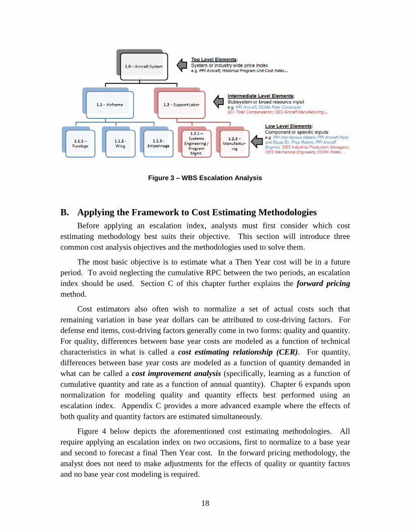
The framework for analyzing escalation can apply to all levels of cost detail. Figure 3 below shows a notional aircraft WBS with potential escalation indexes useful at each level. Instead of asking “what part of the observed RPC is due to price changes in aircraft prices at large?” the analyst asks “what part of the observed RPC is due to price changes in the components or resource inputs to the aircraft?” For example, the analyst might use a Producer Price Index (PPI) for aircraft to understand the market pressures affecting total aircraft system costs. At a lower level of the WBS, the analyst could examine the PPI for aircraft engines, the Employment Cost Index (ECI), market data on engineering salaries, or other indicators of production cost. See Chapter 7 for selecting an escalation index suited to level of cost detail. See Chapter 10 for more information about the example escalation indexes used in Figure 3.

18

Figure 3 – WBS Escalation Analysis

B. Applying the Framework to Cost Estimating Methodologies Before applying an escalation index, analysts must first consider which cost

estimating methodology best suits their objective. This section will introduce three common cost analysis objectives and the methodologies used to solve them.

The most basic objective is to estimate what a Then Year cost will be in a future period. To avoid neglecting the cumulative RPC between the two periods, an escalation index should be used. Section C of this chapter further explains the forward pricing method.

Cost estimators also often wish to normalize a set of actual costs such that remaining variation in base year dollars can be attributed to cost-driving factors. For defense end items, cost-driving factors generally come in two forms: quality and quantity. For quality, differences between base year costs are modeled as a function of technical characteristics in what is called a cost estimating relationship (CER). For quantity, differences between base year costs are modeled as a function of quantity demanded in what can be called a cost improvement analysis (specifically, learning as a function of cumulative quantity and rate as a function of annual quantity). Chapter 6 expands upon normalization for modeling quality and quantity effects best performed using an escalation index. Appendix C provides a more advanced example where the effects of both quality and quantity factors are estimated simultaneously.

Figure 4 below depicts the aforementioned cost estimating methodologies. All require applying an escalation index on two occasions, first to normalize to a base year and second to forecast a final Then Year cost. In the forward pricing methodology, the analyst does not need to make adjustments for the effects of quality or quantity factors and no base year cost modeling is required.

19

Figure 4 – Major Cost Estimating Scenarios and Processes

Analysts should always choose the inflation or escalation index that best

complements the data and methodology. However, it is often preferred to use labor hours to model the cost effects of quality or quantity changes if data permits. Using labor hours removes the need to normalize historical costs to a base year and a potential source of error. The analyst will still have to apply a forward price rate to dollarize the estimated labor hours using a forecasted escalation index.

C. Forward Pricing Suppose a project due to start in 2017 is estimated to cost TY17 $10M. If that

project experienced a two-year delay, and will now start in 2019, what would the TY19 cost be? If the analyst used an inflation index to move between TY17 and TY19, the analyst would neglect real price change and risk mispricing the project. Therefore, an escalation index is recommended to re-phase costs.

To properly escalate the costs to TY19, the analyst will first take the TY17 $100M and normalize (divide) by the 2017 value from the escalation index. The resulting CP$ value will be expressed in terms of prices during the base year. No base year dollar analysis or adjustments are required because project quality and quantities are assumed constant. The CP$ will then be multiplied by the (forecast) 2019 value from the same escalation index and base year, returning the final TY19$ cost.

20

Mechanics of Cost Conversion

How the analyst converts to base or objective year dollars depends on whether the cost data represent expenditures (i.e., outlays) or obligations. The key distinction is that raw indexes are used to convert expenditures (transactions at a specific point in time) and weighted indexes are used to convert obligations (dollars which will be spent over an outlay period). Underlying a raw index is the assumption that appropriated funds are obligated (guaranteed) and expended (paid for) in a single year. When appropriated funds are obligated in one year, but expended over a number of years, a weighted index is used to account for price change that occurs in those subsequent years. Note that the concepts are the same whether converting costs using an inflation index (via CY$) or escalation index (via CP$). See Appendix F for additional information.

In most cases, analysts should not rely on DoD-published indexes to measure escalation. For example, the Research, Development, Test, and Evaluation (RDT&E) and Procurement indexes reflect inflation. The indexes take appropriation titles because the weighted index version reflects their generalized expenditure rates (via outlay profiles). They do not reflect DoD pricing experience or industry analysis. However, DoD-published indexes provide escalation indexes for at least four spending categories: military pay, civilian pay, fuel, and medical. See Chapter 9 for additional information on escalation and inflation indexes published by DoD.

Although escalation in a given program may match a DoD index, this conclusion should be supported with analysis. Professional market studies, cost estimating models, government-published price indexes, contractors’ forward pricing rate agreements, contractual economic adjustments, historical quality-adjusted unit costs, and historical labor rates are among the preferred data and tools to measure past and forecast future escalation. See Chapter 10 for additional information on escalation resources.

Often, the analyst will not have insight into the escalation assumptions used to develop the original Then Year cost estimate. Continuing the example, the analyst may need to re-phase the TY17 $10M to TY19, but has no documentation for the original escalation index used. Further, the original estimate may have been performed using a detailed build-up using many escalation indexes. Where the analyst lacks insight into the assumed escalation for a cost figure, the analyst should draw from the best information available to apply an escalation index that does better than inflation alone. The situation highlights the importance of documenting escalation assumptions to assist future updates to cost estimates, discussed in Chapter 8.

D. Forecasting Prices Beyond the Future Year’s Defense Program Cost estimates usually require assumptions about future inflation and price

escalation rates. The DoD-published indexes will typically provide forecasts for a five-year period called the Future Years Defense Program (FYDP). Similarly, forward pricing rate agreements between the DoD and industry partners typically only extend out five years. Because many program estimates have spending requirements beyond five years,

21

the analyst should determine long-term assumptions that maximize the realism and stability of the cost estimate.

Standard practice has been to apply the percentage growth rate from the last year of the FYDP to all subsequent years. For example, if the forecasted growth rate for the fuel appropriation in the fifth and final year of the FYDP were 1.00%, the analyst would assume annual 1.00% growth for fuel in the sixth, seventh, and eighth years, and beyond. Neither the Office of Management and Budget nor OUSD (Comptroller) currently require analysts to extrapolate price growth assumptions for the last year of the FYDP into out years beyond the scope of the guidance.6 The practice causes disruptive changes in cost estimates that are updated annually, based solely on FYDP rates. Estimates of programs with large sustainment costs, normally incurred over many decades, are made particularly unstable. Guidance for fuel is especially volatile. Between fiscal years 2001 and 2016, the fuel escalation rate in the last FYDP year ranged between -0.9% and 2.7%. Extrapolation of these rates over a twenty year window, shown in Figure 5, can create substantially different conclusions about future price levels.

Figure 5 – Extrapolating Fuel Prices Using Last Year of FYDP

6 For the President’s Budget, OUSD(C) guidance had previously prescribed use of the growth rate from the

last year of the FYDP in all out years. OUSD(C) removed this guidance in FY 2012. However, in FY 2017 OUSD(C) stipulated that for military and civilian pay raises only, the growth rate from the last year of the FYDP was to be applied “for 2021 and beyond”.

0.60

1.00

1.40

1.80

Inde

x, 1

.00

= La

st Y

ear o

f FYD

P

22

Not all escalation indexes will have forecasts, and those that do may not forecast out far enough. While it is preferred to use a professional forecast, analysts will at times need to develop their own. The same best practice that applies to OUSD (Comptroller) indexes applies to years beyond other government or commercial forecasts: out year assumptions should be chosen to maximize the realism and stability of the estimate. There is no right way to forecast a price index. Some may use a line-of-best-fit from historical data. Others may carry forward the average actual RPC over the GDPPI forecast. Others still may model supply and demand factors or employ Markov chains. Do not, however, automatically extrapolate the last forecast rate out into the indefinite future. In the same way that cost analysts (and the organizations publishing estimates) are responsible for determining appropriate escalation indexes for a given analysis, they are also responsible for creating defensible forecast assumptions using the best information available.

For most long-term forecasts, this Handbook recommends using professionally published rates. (See Chapter 10 and Appendix J for forecasting resources.) Although estimating future rates from historical data may be appropriate, the further into the out years the analyst estimates the more uncertainty will come to dominate. As a result, this Handbook recommends setting long term escalation rates (forecasts more than five years out) at the at the Federal Reserve’s inflation target, currently two percent per annum.7 Long term rates different than the inflation target credibly set by the Federal Reserve should be used when supported by defensible analysis. For example, where labor costs are under consideration, a reasonable long term rate forecast would be about one percentage point above inflation. This is because labor wages as measured by the Employment Cost Index (ECI) have outpaced inflation over the long term, representing returns to increasing labor productivity over time. However, where the analyst chooses to estimate higher long term rates due to labor productivity, the analyst should incorporate symmetric logic such that output-per-hour also increases, requiring fewer overall hours to produce the same constant quality item.

7 The Federal Reserve currently targets a two percent inflation rate to be “consistent over the longer run”

with its dual mandate for “price stability and maximum employment.” https://www.federalreserve.gov/faqs/economy_14400.htm.

23

5. Normalizing for Decision Support

Constant Year and Constant Price figures convey distinct information and have different uses in cost analysis. If the dollar can be viewed as a measuring stick for expressing the cost of all items, inflation “lengthens” the measuring stick. Constant Year dollars (CY$) attempt to remove the distortion caused by changes in the measuring stick, but preserve real price change. Real price change (RPC) signals increasing or decreasing claims against budgetary resources. In contrast, Constant Prices (CP$) can sometimes serve as indicators of changes in quantity or capability underlying Then Year dollar costs.

Analysts should always assess escalation when creating TY$ cost estimates. However, when necessary to present a cost estimate for decision making in terms of a “reportable” base year, the conversion from Then Year dollars to Constant Year dollars should be made with an inflation index, not an escalation index. This principle applies to life cycle costs for all appropriations and phases of the program. Chapter 9 discusses published DoD inflation indexes which provide authoritative guidance for Constant Year conversions to a “reportable” base year.

This chapter will help analysts understand the best practice of presenting cost estimates to support decision making in Then Year or Constant Year dollars, but not Constant Prices. Cost figures not only convey information about a specific program or cost element, but facilitate the comparison of alternatives. Constant Year dollars provide a consistent normalization process that enables direct comparisons, and are useful for decision support. Common cost comparisons include, but are not limited to: affordability analyses (Section A); comparing alternative purchases (Section B); and comparing current and baseline costs to measure program performance (Section C).

A. Affordability Analysis A reliable affordability analysis is critical to understanding whether program

funding needs fit under a future budget. An aggregate portfolio of cost estimates, combined with all other fiscal demands, must not exceed a reasonably projected topline budget. Guidance finds a reasonable projection of the topline to grow by inflation as measured by the GDPPI.8

Suppose DoD is executing two programs, A and B, and wants to assess the affordability of a new program, C. The programs use a unique mix of market resources,

8 See Defense Acquisitions University (DAU), section 3.2.2. – Affordability Analysis.

https://acc.dau.mil/CommunityBrowser.aspx?id=488335&lang=en-US.

24

the prices of which are expected to grow faster than the prices of resources in the economy as a whole. Assume program cost estimates reflect realistic escalation assumptions.

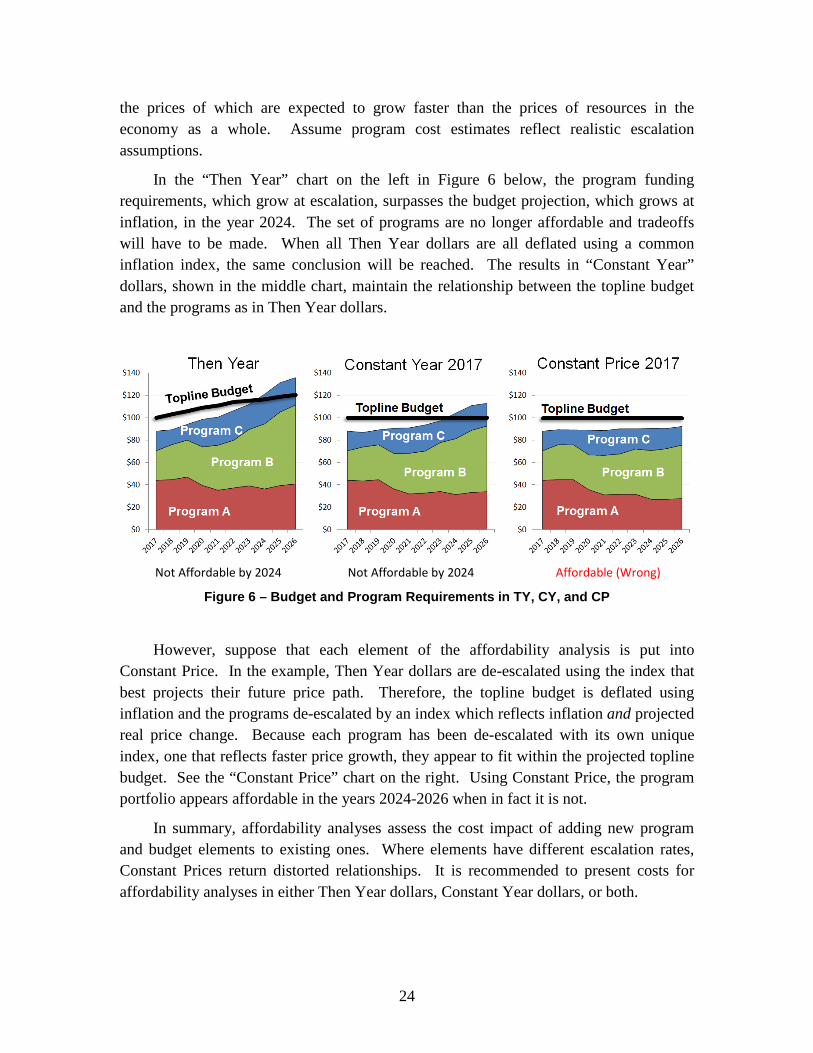
In the “Then Year” chart on the left in Figure 6 below, the program funding requirements, which grow at escalation, surpasses the budget projection, which grows at inflation, in the year 2024. The set of programs are no longer affordable and tradeoffs will have to be made. When all Then Year dollars are all deflated using a common inflation index, the same conclusion will be reached. The results in “Constant Year” dollars, shown in the middle chart, maintain the relationship between the topline budget and the programs as in Then Year dollars.

Not Affordable by 2024 Not Affordable by 2024 Affordable (Wrong)

Figure 6 – Budget and Program Requirements in TY, CY, and CP

However, suppose that each element of the affordability analysis is put into Constant Price. In the example, Then Year dollars are de-escalated using the index that best projects their future price path. Therefore, the topline budget is deflated using inflation and the programs de-escalated by an index which reflects inflation and projected real price change. Because each program has been de-escalated with its own unique index, one that reflects faster price growth, they appear to fit within the projected topline budget. See the “Constant Price” chart on the right. Using Constant Price, the program portfolio appears affordable in the years 2024-2026 when in fact it is not.

In summary, affordability analyses assess the cost impact of adding new program and budget elements to existing ones. Where elements have different escalation rates, Constant Prices return distorted relationships. It is recommended to present costs for affordability analyses in either Then Year dollars, Constant Year dollars, or both.

25

B. Comparing Alternative Purchases Programs often have multiple courses of action available to fulfill mission

requirements. Decision makers must select the most effective alternative taking into account differences in cost, schedule and technical requirements. Consider the following example that focuses on aspects related to cost. A system that is deployed in fiscal year 2017 can undergo depot overhauls in two year cycles with equal reliability using either a “Labor Intensive” option or a “Material Intensive” option. Assume for simplicity that the discount rate is zero percent.9 The cost estimator’s task is to determine the most cost effective option over a 15 year timeframe and make a recommendation to decision makers.

Table 2 – Summary of Alternatives

Labor Intensive Material Intensive

Time between depot overhauls 2 years 2 years

Cost of depot overhaul in FY'17 $20.0K $25.0K

Forecasted escalation rate 7.00% 3.00%

Which alternative is recommended? Over 15 years, the system would undergo seven overhauls under both alternatives. By correctly applying forecasted escalation (not inflation) to the current cost of each alternative, the analyst will return the cumulative Then Year overhaul cost profiles (left chart of Figure 7 below). The 15-year sustainment costs are $217K for the Material Intensive option and $233K for the Labor Intensive option. In Then Year dollars, the Material Intensive option appears marginally more cost effective.

Then Year dollars, however, are not appropriate for comparing alternatives with different expenditure patterns over time due to the fact that options might use different escalation rates. Remember that the purchasing power of the dollar is also changing over time. To account for the different timing of expenditures across options, the effects of the change in the dollar’s purchasing power must be removed. Deflating the stream of

9 Suppose the analyst was to use a discount rate. Provided that the analyst used the escalation framework

to derive final Then Year costs, there are two general methods for discounting: 1) discount future TY$ cash flows using the nominal discount rate; or 2) convert the future TY$ cash flows into CY$ using an inflation index and discount using the real (inflation-adjusted) discount rate.

26

overhaul costs for each alternative by a common inflation index returns Constant Year dollars in the base year of FY17 (middle chart of Figure 7 below).

After deflating Then Year to Constant Year dollars, the analyst finds a Material Intensive overhaul cost of $188K and a Labor Intensive cost of $199K. The conclusion remains; the Material Intensive option is marginally more cost effective when viewed in Constant Year dollars. However, different conclusions are often reached between Then Year and Constant Year dollars, which may have been the case in this example if the alternatives had different overhaul cycle times, or had a significant discount rate been applied.

Marginally Favor Labor Marginally Favor Labor Strongly Favor Materials (Wrong)

Figure 7 – Alternative Cum. Cost Profiles in TY, CY, and CP

While Then Year costs are best estimated utilizing escalation, the analyst should present alternative costs in Constant Year dollars because it preserves the effects of real price change, which often differ between alternatives. The Labor Intensive option is more expensive because its projected escalation rate is four percentage points higher than for Material. Should the analyst normalize the Then Year dollars to Constant Prices (right chart of Figure 7 above), it would remove all real price growth, distorting the comparison. De-escalating the Material Intensive option with a 3.0% annual escalation index and de-escalating the Labor Intensive option with a 7.0% annual escalation index would lead the analyst to the wrong conclusion. It incorrectly presents the Labor Intensive option as significantly less expensive, as opposed to marginally more expensive, compared to the Material Intensive option.

Constant Year dollars are the appropriate method for presenting the stream of costs in an analysis of alternatives. Decision makers need to understand which alternative is more cost effective after removing distortions to the “measuring stick,” or purchasing

Then Year Constant Year Constant Price

Cum

ulat

ive

Cost

s, $

K

27

power of the dollar, caused by different expenditure time-phasing. Constant Prices remove additional information about real price changes, and therefore prohibits an accurate comparison of alternatives relative to actual budgetary demands.

C. Measuring Program Performance Program performance is often measured relative to a baseline cost objective, and

growth above certain thresholds trigger additional controls and oversight. Cost performance baselines and metrics should be expressed in Constant Year dollars converted using the GDPPI (weighted, as necessary, according to the outlay profile for the type of appropriation being costed). Differences across cost estimates, including changes compared to baseline, are best presented in Constant Year dollars for two primary reasons.

First, Constant Year dollars are a focal point. Each observer can immediately recognize that the dollars were converted using the GDPPI, and draws the same interpretation. Constant Prices are converted using an escalation index, but beg the question “an escalation index of what?” An escalation index might measure the price change for a broad basket of goods, such as all aircraft manufacturing inputs, or a narrow basket, such as titanium. Proper interpretation of Constant Prices requires further investigation into the escalation index.

Second, and more importantly, Constant Year dollars preserve the appearance of real price change (RPC) which is often important information for detecting, and acting on, changes in program costs. Suppose two program baselines were estimated with different escalation assumptions, one with a real price change of positive 3.00% and the other negative 3.00%. If both programs experienced annual cost growth 2.00% above the baseline escalation assumptions, different views emerge in Constant Year dollars and Constant Prices. A Constant Year profile (left-hand side of Figure 8 below) will reflect the fact that the second program demanded fewer real resources over time, despite experiencing cost growth, while the first demanded ever increasing resources. A Constant Price profile (right-hand side of Figure 8 below) only shows performance to assumptions, or the fact that both programs experienced annual cost growth of 2.00% above baseline.

28

Figure 8 – Presenting in Constant Year and Constant Price

Not only will the audience’s perception of program costs differ depending on the method of cost conversion, but so will the calculated average unit cost growth. While the percent growth in Figure 8 is exactly the same between the two programs in Constant Prices, they differ in Constant Year dollars. Because both programs experienced an equal 2.00% annual RPC above baseline escalation assumptions, they realized the same percentage cost growth in CP$ (11.77%).10 Yet when measured in CY$, Program 1 shows relatively higher percent cost growth and Program 2 relatively lower (12.55% and 10.97%, respectively). This differential occurs because Program 1 had assumed positive RPC in the baseline while Program 2 assumed negative RPC. The higher baseline escalation assumptions translated into higher percent cost growth in Constant Year dollars due to the effects of compounding growth.

Cost growth measured in Constant Prices is not recommended because every commodity, possibly every program, could use its own unique measure of success. Constant Prices further distort the opportunity costs of actual dollars the DoD has

10 Had the programs used escalation indexes that depended in large part on the programs in question, there

would have been 0.00% cost growth in Constant Prices. Say that these programs represented the only purchases in their commodity group, and the escalation indexes at the time of baseline, based on previous program actuals, get filled in with the actuals from the programs in question. In this case, the final escalation indexes would have incorporated the higher real price change than forecasted and normalized away any apparent cost growth. It was assumed here that the programs in question did not affect the realized escalation indexes, which conformed to escalation forecasts at the time of the baseline.

Shows some RPC: removes RPC reflected in the escalation index, highlights RPC above assumptions

Shows all RPC: highlights increasing or decreasing claims on government resources

29

The Selected Acquisition Report (SAR) Process

Each military department submits to OUSD(AT&L) the updated cost estimates of each major defense acquisition program (MDAP) in then year dollars, and a set of price indexes applicable to each appropriation. The SAR reporting system calculates the cost performance metrics, including conversion of the cost estimates from then year to base year dollars. The process for Operating and Support (O&S) costs differs because the services convert those costs to constant base year dollars before they are submitted to OUSD(AT&L).

available. The example programs have the same average cost and percent growth in Constant Prices. In Constant Year dollars, however, one program shows decreasing demands on the DoD’s budget which allows for more programming while the other shows increasing demands that may require cuts there or elsewhere. For these reasons, programs that assume a faster escalation rate in the baseline should undergo closer scrutiny.

30

6. Normalizing for Cost Estimation

This chapter will provide examples of how the choice of index, whether inflation or escalation, can affect cost estimates. Two common methodologies will be explored: cost estimating relationships and learning curves. The former models how system costs are affected by the attributes of a system – its quality. The latter models how unit costs are affected by the number of units produced – its quantity. In both cases, the modeling occurs on cost data normalized to an “analytical” base year. It will be shown that Constant Prices are the preferred base year units in which to perform such analyses, as opposed to Constant Year dollars. The intent of this chapter is to supplement, and not replace, existing cost estimating training with a focus on the impact of normalization assumptions.

A. Normalizing for Cost Estimating Relationships (CERs) A cost estimating relationship (CER) is a parametric model that seeks to determine

the statistical relationships between program costs and the characteristics of sampled weapon systems. Cost analysts use CERs to predict the cost of a future program given its (planned) characteristics. The following example will introduce how the cost normalization choice affects the estimated relationships for a given set of data.

Suppose an analyst is estimating the Detail Design phase for a new ship, slated to start in 2019, based on actual costs for analogous programs. For simplicity, assume weight (measured by full-load displacement in thousands of long tons) is the sole cost-driver. During Detail Design, the Department primarily buys labor to solve system design problems, and often the assumption is that the relationship exists between the cost-driver (weight) and the amount of resources (i.e., the number of labor hours). In this example, ship design resource costs have escalated at 3.5% as opposed to 2.0% for the economy-wide measure of inflation. Normalizing Then Year dollars with escalation will remove price escalation in ship resource costs, revealing the “true” underlying relationship between resources and weight. Table 3 below shows the available information for six analogous programs.

31

Table 3 – Analogous Program Information

Assumptions: Inflation = 2.0%, Escalation = 3.5%

Start Year

(A) (B) (C) (D) (F) (G) Ship

Weight (K LT)

Then Year $M

Escalation Index, Wtd.

Constant Price 2017 $M

(B ÷ C)

Inflation Index, Wtd.

Constant Year 2017 $M (B ÷ F)

1990 25 $215.2 0.422 $510.0 0.609 $353.6 1992 12 $113.0 0.452 $250.0 0.633 $178.4 1998 10 $116.7 0.556 $210.0 0.713 $163.6 2000 7 $89.3 0.595 $150.0 0.742 $120.3 2005 15 $219.1 0.707 $310.0 0.819 $267.5

Because escalation in ship design resource costs has outpaced inflation, historical programs’ costs viewed in 2017 Constant Prices are higher than in 2017 Constant Year dollars. The cost as a function of weight scatterplot is shown in Figure 9 below, and highlights the different views of the relationship. Note that the CER performed in Constant Year dollars returns a shallower slope (an additional 1,000 tons of weight costs CY17 $13.2M vice CP17 $20M).

Figure 9 - Cost Estimating Relationships

1990

1992 1998 2000

2005

$-

$100

$200

$300

$400

$500

$600

5 10 15 20 25 30

Deta

il De

sign

Pha

se C

ost,

$M

Weight (K)

Constant Price 2017 CP17$ = 10 + 20*Weight

Constant Year 2017 CY17$ = 34.5 + 13.2*Weight

Then Year Actuals

32

The example data assumes that ship weight has a perfect linear relationship with the analogous Detail Design phase costs when measured in Constant Prices. The relationship exists between weight and escalation-adjusted Constant Prices, and not inflation-adjusted Constant Year dollars, because it is assumed that ship development of a given weight requires a certain amount of labor resources, not dollars.11 The relationship takes the form:

𝐶𝐶𝑃𝑃17$ = 𝐼𝐼(𝑊𝑊𝑅𝑅𝐼𝐼𝑎𝑎ℎ𝐼𝐼) = $10𝑀𝑀 + $20𝑀𝑀 ∗𝑊𝑊𝑅𝑅𝐼𝐼𝑎𝑎ℎ𝐼𝐼 (𝐾𝐾 𝐿𝐿𝐿𝐿) + ɛ

The equation states that ship Detail Design would cost on average $10M in 2017 Constant Prices plus $20M for each additional 1,000 tons. (The epsilon reflects a standard error term reflecting all other factors not accounted for by weight.) If the new ship program is planned to weigh 30,000 tons, the Constant Price CER would predict a cost of ($10M + $20M · 30K LT) = CP17 $610M. The Constant Year Dollar CER, however, would predict a cost of ($34.5M + $13.2M · 30K LT) = CY17 $431M. If execution of the Detail Design effort was to start in the year 2017, the Constant Year Dollar CER would underestimate the costs by 29%. However, we assume Detail Design starts in 2019. Therefore, multiplying the Constant Price and Constant Year costs by the forecasted 2019 value of their respective weighted indexes returns the final Then Year Detail Design costs ($674M vice $456M). The Constant Price CER predicts a Then Year cost 32% higher than the Constant Year CER, the difference increasing due to anticipated real price change.

The results can be generalized for any bivariate linear CER. For multiple data points, the precise relationship is dependent on how the cost-driver is correlated with time (which it often is). We can derive a rule of thumb by considering a single data point, known as an Analogy estimate. Assuming a relationship between cost-driver and Constant Prices that is perfectly linear (an assumption that will not hold in practice), the error of an individual analogy using a Constant Year CER is fully described by the age of the Then Year cost data and the real price change over that time. Figure 10 below shows the analogy error as a function of age for select RPC values, where inflation and RPC have had constant growth rates. For example, suppose an analogy is 30 years old in a commodity that has experienced a constant +2% annual RPC. In this case, costs as calculated by Constant Year dollars are expected to be 45% lower than costs as calculated by Constant Price.

11 It would also be valid to apply an escalation index measuring the quality-constant costs of

“representative” Detail Design outputs (e.g., ship engineering documents and models from past programs) as opposed to an escalation index measuring project inputs (e.g., labor costs). This application assumes the underlying relationship exists between ship weight and dollars, but such escalation indexes for unique defense outputs often do not exist. Analogous commercial indexes may also be lacking. See Chapter 7 for additional insight on selecting the proper escalation index.

33

Figure 10 – Analogy Error as Function of Time by Real Price Change (RPC)

Note that for positive RPC, the percent underestimated increases with age at a decreasing rate. For negative RPC, the percent overestimated increases with age at an increasing rate. This is because underestimates of 50% and 75% are equivalent to overestimates of 100% and 400%, respectively. In the extremes, positive real price changes can create underestimates that are asymptotic at 100% while negative real price changes can create overestimates that approach infinity. For a more advanced example of escalation application into CERs, see Appendix C.

B. Normalizing for Learning Curve Analyses The previous section addressed the CER and Analogy cost estimating techniques for

adjusting for quality; this section addresses adjusting for quantity. When line workers perform repetitive tasks in the production of large complex end items in an environment of continuous pressure to reduce costs, they learn to become more efficient in their processes, resulting in fewer direct labor hours needed to produce each subsequent item. This learned efficiency (measured in labor hours or the cost thereof) can be plotted on a chart and a “learning curve” observed. Experience shows that for every doubling of cumulative production quantity, touch labor hours tends to decrease by a fixed percent. When analyzing labor costs, the data must be normalized to adjust for effects that expose learning that occurs on labor hours. The example below will discuss how the method of

-80%

-60%

-40%

-20%

0%

20%

40%

60%

80%

0 5 10 15 20 25 30

Anal

ogy

Estim

ate

% E

rror

Age of Then Year Cost Data

+4% RPC +3% RPC +2% RPC

+1% RPC

-1% RPC

-2% RPC

0% RPC

34

cost normalization affects future projected cost savings from learning based on analysis of historical data from an analogous program.

Using the analogous data set, the cost estimator must determine the cost of seven new annual production lot buys that span years 2018-2024. Assume that the analyst has targeted Integration, Assembly, Test, and Checkout (IAT&C) costs, and that the analogy’s parameters are expected to be same as the new program in all important respects.12 Further, assume that labor costs are known to be $10 per hour in 2017, which has experienced, and is expected to continue experiencing, 2.00% real price change over a 2.00% inflation rate (or an escalation rate of 4.04%).

With information on hours, the estimator would regress the hours-per-unit against the quantities and estimate a learning slope of 87.4% and a T1 cost of 157 hours. This “Full Insight Model” estimates IAT&C labor hours as a function of cumulative quantity, the proper objects of learning. Projected labor rates can then be applied to estimated hours to derive a total cost. See Table 4 below.

Table 4 – Analogous IAT&C Data and Learning Curve Coefficients

Lacking data on hours, the estimator can use the dollars-per-unit to back into the underlying learning which occurs on labor hours. Because the purchasing power of the dollar has changed over time, the analyst cannot estimate the learning on Then Year

12 Important similarities include: 100% of the costs are in recurring touch labor; same performing

contractor; zero productivity change; the theoretical first units (T1) require the same number of labor hours; annual buys of 20 units; annual buys fully executed within one year; no production breaks or requirement changes.

35

dollars. An hour of labor today almost certainly costs a different amount in Then Year dollars than an equivalent hour of labor five years ago. The estimator can normalize the dollars in two principal ways:

1) Inflation Model – use an inflation index to remove distortions to the purchasing power of the dollar relative to an economy-wide basket of goods and services

2) Escalation Model – use an escalation index to remove distortions to the purchasing power of the dollar relative to the analogous program’s labor costs

Note that in Table 4 the estimated IAT&C learning slope in Constant Prices agrees with the Full Insight Model using hours. The T1 costs also agree, though the units have different denominations. Using Constant Year dollars, both the estimated learning and T1 cost are less. This is because the price of labor grew faster than inflation. As a result, the Escalation Model found a dollar in the past bought relatively more labor hours than the Inflation Model. More implied hours in the past means the program experienced relatively steeper (greater) learning. Figure 11 below shows a plot of the analogous data set in Then Year dollars (black). It also shows the fitted, or regression derived, values from the Escalation Model (CP17$, blue) and Inflation Model (CY17$, red).13

Figure 11 – Analogous Data Fitted Values

13 A further indication that the Inflation Model is problematic is that the red curve does not pass through

the actual 2017 value, despite the “perfected” data concocted for this example.

$400

$600

$800

$1,000

$1,200

2011 2012 2013 2014 2015 2016 2017

Uni

t Cos

t

Escalation Model (CP17$) Learning = 87.4% ; T1 = 1,571

Inflation Model (CY17$) Learning = 89.9% ; T1 = 1,265

Then Year Cost Data Avg. Hours * Escalated Hourly Labor Cost

36

The coefficients from the analogous learning models can also be used to predict the new program’s costs in both Constant Year dollars and Constant Prices. The predicted values from the regression models, which remain in base year 2017 dollars, are still expressed in different types of dollars. The Escalation Model is in CP17$ and the Inflation Model in CY17$. The predicted costs for the new program are displayed in Figure 12 below, and shown relative to the predictions from the Full Insight Model (performed on labor hours) in TY$ in purple.

Figure 12 – New Program Predicted Values

The final step is to convert all predicted costs to Then Year dollars. This is done by applying the projected inflation index values to the Constant Year dollars and the projected escalation index values to the Constant Prices for 2018-2024. See Figure 13 below. Note that the estimate performed using the Escalation Model agrees with the Full Insight Model. The complete agreement is because labor costs alone were targeted and perfect information regarding escalation was assumed. The Inflation Model, on the other hand, underestimated unit costs relative to the Full Insight Model by more than 10%.

$400

$600

$800

$1,000

$1,200

2018 2019 2020 2021 2022 2023 2024

Uni

t Cos

t

Inflation Model (CY17$) Learning = 89.9% ; T1 = 1,265

Escalation Model (CP17$) Learning = 87.4% ; T1 = 1,571

Full Insight Model (Hours) Learning = 87.4% ; T1 = 157.1 TY$ = Hours * Escalated Labor Cost per Hour

37

Figure 13 – New Program Final Then Year Cost Estimates

In the case where an analogous historical program is used to estimate a future program, the Inflation Model will produce Then Year costs which preserve much the same slope relative to the Escalation Model. The slope is largely preserved because the regression in Constant Year dollars seeks to produce a mean bias of zero over the relevant quantities. The Inflation Model’s Then Year costs fall below the Escalation Model’s because it neglects the real price change that has occurred between the analogous program and the new. Had the objective been to estimate new buys for the same program, as opposed to the same buys for a new program, the Inflation Model would show different patterns of estimate biases. See Appendix D for a learning curve example using program actuals instead of an analogy.

Because information regarding past and future escalation rates is often noisy, it is recommended that cost estimators seek to use effort (labor hours) data whenever possible for estimating learning curves. The Escalation Model learning curve is a second-best method when only costs (dollars) are available and labor costs can be targeted. The Escalation Model seeks to strip away noise in the change of the dollar’s purchasing power relative to the proper object of learning curve analysis, labor hours.

$400

$600

$800

$1,000

$1,200

2018 2019 2020 2021 2022 2023 2024

Full Insight Model (TY$) TY$ = Hours * Escalated Labor Cost per Hour

Escalation Model (TY$) TY$ = CP17$ * Escalation Index (BY17)

Inflation Model (TY$) TY$ = CY17$ * Inflation Index (BY17)

38

7. Selecting an Escalation Index

When estimating a particular program or cost element thereof, the analyst should use the price index that best represents the program’s actual or anticipated experience. Because there is no “one size fits all” approach, this chapter provides considerations that will help the analyst choose the appropriate escalation index for a given objective.

A. Index Attributes A spectrum of escalation indexes is available. The analyst can normalize cost data

for an item using an index derived from its own unit costs. Such an extremely precise escalation index will be called the “own” index, which the analyst must often derive from primary data sources. Conversely, the analyst may broaden the scope of items included in the index so wide that that the escalation index becomes tantamount to inflation. Between the two extremes is a range of indexes containing varying degrees of representative items. A “representative” escalation index is constructed, often by a professional source, from the cost of analogous items which may be precisely or imprecisely defined around the characteristics of the historical cost data of interest. This Handbook finds relatively precise “representative” indexes based on actual defense costs, while relatively imprecise “representative” indexes are based on commercially available prices. Figure 14 below provides example index spectrums applicable to certain cost normalizations. See Chapters 9 and 10 for more information about the indexes below.

Figure 14 – Spectrum of Price Indexes

Just as the uses of Constant Year dollars and Constant Prices differ, so do the uses of Constant Prices normalized using the “own” and “representative” escalation indexes. While the “own” index returns the flat unit cost streams, removing all real price change,

39

the “representative” index preserves some, but not all, real price change.14 This is because the representative index approximates the price change, but includes additional “noise” because it also includes price changes from items similar, but not identical, to the item of interest.

It is important to consider whether adjustments have been made to the escalation index when using Constant Prices. Chapter 2 defined an escalation index as quality-adjusted, which means price changes resulting from improvements in the item’s capabilities are excluded. A quality-adjusted escalation index is used to normalize costs of similar items of differing technical characteristics. Remaining variation in the resulting Constant Prices of the items can be attributed to differences in technical characteristics using a CER. Many defense and commercial escalation indexes are quality-adjusted; indexes of labor costs, often unadjusted, are a major exception (see Chapter 10).

Cost improvement through learning and rate effects are important concerns in many defense purchases. If historical cost data displays cost improvement, the analyst requires not only a quality-adjusted escalation index, but one that is also quantity-adjusted. Such a quality- and quantity-adjusted escalation index would result in Constant Prices whose remaining variation can be attributed to differences in quantity demanded as well as in technical characteristics. However, attribution of Constant Price variation between relevant quality and quantity factors can be hard to disentangle. For this reason, cost improvement analyses are best performed on constant-quality items such that the whole of the Constant Price variation can be attributed to quantity demanded.

When using a relatively precise “representative” escalation index of similar defense end items to analyze quality or quantity factors, the index must always be both quality- and quantity-adjusted.15 The analyst may also normalize defense cost data using a relatively imprecise “representative” escalation index of commercially available analogous items. Many commercial escalation indexes, though quality-adjusted, are not quantity-adjusted.16 For normalizing defense costs, however, they need not be quantity-adjusted. Commercial markets, unlike their defense facsimiles, bring together numerous

14 Note that the “own” index, being precisely defined, can only normalize cost data to years within the

range that the specific item was produced. To create a consistent escalation index over long periods of time, especially important in defense because the underlying characteristics within and between programs change frequently, a “representative” index must often be derived from analogous items.

15 Productivity adjustments can be made, for example, by only factoring costs after the 100th unit of production where learning effects are less (if production rates are relatively low).

16 Not quantity-adjusted with respect to learning and rate effects, that is. However, some commercial escalation indexes are seasonally-adjusted, a form of quantity adjustment due to the effects of supply or demand factors resulting from seasonal changes (particularly important for agricultural products).

40

buyers and sellers. The price does not depend on the demand decisions of one primary buyer as it does in defense, where quantity orders are often small and learning/rate effects often significant. Therefore, a “representative” escalation index of commercial analogues can be considered quantity-constant with respect to learning and rate effects.

B. Index Selection The selection of an “own” or “representative” escalation index, and whether it

should be quality-adjusted, quantity-adjusted, or even in some cases unadjusted, depends upon the cost analyst’s objectives. Objectives can often be accomplished through a number of valid approaches. This Handbook will suggest two primary approaches to guide index selection across the range of possible alternatives.

When assessing historical data for cost estimates, whether actuals from the program under consideration or analogous programs, the analyst will often consider the costs as either an output or a combination of inputs. For example, in the CER example presented in Chapter 6, the historical cost data pertained to the Detail Design of Navy ships. While the output could be considered a set of engineering documents and models, the analyst may prefer to consider costs in terms of a production process where the product is the output from combining certain inputs; in this case, labor hours. Approached as an output, the analyst would normalize with an escalation index representing the cost of ship design documentation and models. Approached as an inputs process, the analyst would normalize with an escalation index representing labor hour costs. The CER example in Chapter 6 took the latter approach.

What are the interpretations of cost data normalized in these two ways? For the output approach, the normalized data represents the cost of that particular set of ship engineering documents and models as if they were developed and bought in the base year of the escalation index. For the inputs approach, the normalized data represents the cost of the number of labor hours it required to plan and design that particular ship, if the labor was all bought and expended in the base year of the escalation index.

In most circumstances, the cost analyst finds it preferable to use the output approach. For example, when estimating the cost of a computer, the analyst would naturally like to have an escalation index of computer prices. The analyst would not want to complicate the analysis by isolating and estimating input costs to the computer production process. Taking the output approach for more complex systems, the analyst favors the “representative” escalation index to the “own”. This is because the “own” index returns a flat profile of Constant Prices, removing all appearance of cost changes due to technical characteristics or cost improvement which are often the analyst’s primary interests.

41

The unique environment of defense, however, makes it difficult to derive the favored quality- and quantity-adjusted “representative” index of defense outputs. Attributing price changes between the relevant factors is difficult in defense due to small quantity orders within programs and vast technical differences between programs. While the analyst favors normalizing an output’s costs with a quality- and quantity-adjusted “representative” index, such indexes for defense purchases often do not exist or reflect great uncertainty regarding the true escalation rates. The analyst has three recourses: first, use a quality-adjusted commercial escalation index that may not be indicative of military escalation, but likely does a better job than normalizing for inflation alone; second, segregate the total system into smaller, less complex, outputs using the Work Breakdown Structure (WBS) and apply appropriate escalation indexes; and third, take the inputs approach.

Using the inputs approach, the analyst considers the output’s total cost as an aggregation of direct input costs to the production process. Direct inputs can be segregated into two broad categories: labor (e.g., engineering, manufacturing, management) and material (e.g., raw materials, piece parts, tooling).17 Complex defense outputs require numerous processes that combine heterogeneous forms of labor and materials inputs. The analyst would need to isolate costs attributable to relevant inputs and normalize them using distinct escalation indexes. Often, material cost will represent complete items (e.g., propulsion or radar) that may require the output approach of escalation normalization. However, where detailed cost data exist for materials through subcontractor reports, the materials may also be approached as a combination of inputs.

When normalizing input costs, the analyst favors using an escalation index derived from the actual price paid per unit. Such an escalation index is its “own” escalation index, rather than a “representative” of similar input costs (more desirable for normalization in the output approach). Normalization for the cost of one unit of an input over time using an “own” index, unadjusted for either quality or quantity, should return the idealized flat stream of Constant Prices. Normalizing aggregate input costs using the unadjusted “own” index should return a stream of Constant Prices that reflect the relative number of inputs bought. For example, normalizing aggregate labor costs using an index of the unadjusted labor rate actually paid will return costs that have the same relative behavior as labor hours.18 The example in Chapter 6 showed that the learning curve slopes calculated on labor hours and de-escalated labor dollars were equivalent.

17 The suppliers’ costs can be segregated into direct and indirect costs. In defense contracts, allowable

indirect costs are allocated to contracts using negotiated factors and rates. 18 Practice has often been to make no adjustments to labor quality in CER or learning curve analyses (by

controlling for non-quantity related productivity or demographics). Unadjusted indexes may hold for defense because suppliers often freeze technology and processes at the start of production. However,

42

Taking the inputs approach, normalization with the “own” index returns the relative quantity of inputs used. It makes no account for whether there were quality differences in the inputs or production processes over time. Because the inputs approach isolates unit resource costs, they never need quantity adjustments. Output costs, rather than inputs costs, are affected by cost improvement. The “representative” index, though applicable to normalizations using the inputs approach, is a second-best method compared to the “own” index as it will return only approximate resource utilization.

Figure 15 below summarizes the flow of considerations for selecting an escalation index. The output approach requires a “representative” index in all cases except forward pricing, where an “own” index is also applicable. If defense procurements comprise the underlying data for the index, the output approach requires a quality- and quantity-adjusted index. If commercial procurements comprise the underlying data, the output approach requires quality-adjustment alone.

The inputs approach favors the “own” index in all cases, though the analyst may also apply a “representative” index. Because the inputs approach seeks relationships in production resource usage, it requires an unadjusted escalation index. Though not depicted in Figure 15, quality-adjusted indexes are applicable to the inputs approach if the analyst determines that the resources purchased include quality improvements that allows for fewer labor or materials inputs to produce the same output. An alternative adjustment is for the “Total Factor Productivity” of the firm, industry, or economy if the analyst believes that the firm is improving the efficiency with which it combines inputs.

Figure 15 – Selecting an Escalation Index

some scholars advocate productivity adjustments (for example, see W. D. Nordhaus, 2009, “The Perils of the Learning Model for Modeling Endogenous Technological Change”). Such an adjustment was made for so-called “green,” or inexperienced, labor in shipbuilding (see Richard L. Coleman, et al., 2008, “Advanced Learning Model for Shipbuilding”).

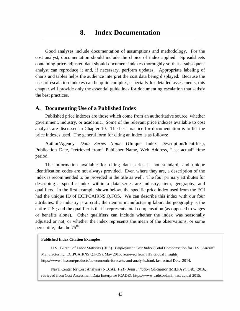
43

Published Index Citation Examples:

U.S. Bureau of Labor Statistics (BLS). Employment Cost Index (Total Compensation for U.S. Aircraft Manufacturing, ECIPCAIRNS.Q.FOS), May 2015, retrieved from IHS Global Insights, https://www.ihs.com/products/us-economic-forecasts-and-analysis.html, last actual Dec. 2014.

Naval Center for Cost Analysis (NCCA). FY17 Joint Inflation Calculator (MILPAY), Feb. 2016, retrieved from Cost Assessment Data Enterprise (CADE), https://www.cade.osd.mil, last actual 2015.

8. Index Documentation

Good analyses include documentation of assumptions and methodology. For the cost analyst, documentation should include the choice of index applied. Spreadsheets containing price-adjusted data should document indexes thoroughly so that a subsequent analyst can reproduce it and, if necessary, perform updates. Appropriate labeling of charts and tables helps the audience interpret the cost data being displayed. Because the uses of escalation indexes can be quite complex, especially for detailed assessments, this chapter will provide only the essential guidelines for documenting escalation that satisfy the best practices.

A. Documenting Use of a Published Index Published price indexes are those which come from an authoritative source, whether

government, industry, or academic. Some of the relevant price indexes available to cost analysts are discussed in Chapter 10. The best practice for documentation is to list the price indexes used. The general form for citing an index is as follows:

Author/Agency, Data Series Name (Unique Index Description/Identifier), Publication Date, “retrieved from” Publisher Name, Web Address, “last actual” time period.

The information available for citing data series is not standard, and unique identification codes are not always provided. Even where they are, a description of the index is recommended to be provided in the title as well. The four primary attributes for describing a specific index within a data series are industry, item, geography, and qualifiers. In the first example shown below, the specific price index used from the ECI had the unique ID of ECIPCAIRNS.Q.FOS. We can describe this index with our four attributes: the industry is aircraft; the item is manufacturing labor; the geography is the entire U.S.; and the qualifier is that it represents total compensation (as opposed to wages or benefits alone). Other qualifiers can include whether the index was seasonally adjusted or not, or whether the index represents the mean of the observations, or some percentile, like the 75th.

44

The “last actual” time period conveys the last observed date recorded in the price index. Some price indexes are forecasts of the future where there is no “last actual” date. In such cases, use “forecast start” and the time period where the price index forecast starts. In other cases, the professional forecast does not extend out long enough, requiring the analyst to perform his or her own forecast. Such instances of extending professional forecasts will be documented as a separate entry that follows the Custom Index style. Composite indexes use multiple sources in some proportion, for example using labor rates from multiple contractors in an industry and weighting them by quantity bought. Where composites are used, simply list the indexes used as if they had been applied independently in the form shown above.

B. Documenting Use of a Custom Index This Handbook provides numerous published escalation resources for the analyst to

apply. They cover most commercial end items and supply-side inputs, such as labor and material. Yet there are often useful data not incorporated into published indexes that are available to the analyst. We do not expect analysts to develop their own price indexes, though such studies are encouraged where sufficient time and manpower can be applied.

Custom indexes come in several forms, but are generally either historical estimates or future extrapolations based on datasets that are either published or unpublished. For example, a time series of labor rates received directly from the contractor would be considered unpublished data, from which a custom index could be derived.

The general form for custom indexes based on published sources is as follows:

“Custom Index based on published data from” Author/Agency, Data Series Name (Unique Data Description/Identifier), Publication Date, “retrieved from” Publisher Name, Web Address, “last actual” time period.

The general form for custom indexes based on unpublished sources is as follows:

“Custom Index based on unpublished data from” Source/Provider, Unique Data Description/Identifier, “retrieved from” Source Contact/Location, “last actual” time period.

C. Labeling Charts and Tables Dollar values in charts and tables should be labeled Then Year, Constant Year, or

Constant Price, and the base year specified if appropriate. All analysts should be able to immediately interpret the former two accurately, when properly labeled. By contrast, Constant Prices require additional information regarding the escalation indexes used to draw the correct interpretation. Each will be discussed in turn.

45

What is a Current Dollar?

One often observes the term “Current” dollars, in some cases used synonymously with Then Year dollars and others distinguished from Then Year dollars based on the outlay profile. In the latter case, Current dollars refer specifically to obligations with an outlay profile of 100% in the first period, in other words expenditures. This Handbook will not recommend one usage for the term “Current” dollar over the other. It will continue to use the term “Then Year” as the general form for both obligations and expenditures. The analyst should always be clear on whether TY$ represent obligations or expenditures.

Then Year. Dollars unadjusted for relative price changes and represent the actual amount of dollars needed at a point in time to meet an obligation or expenditure. If the figure makes the time-phasing of Then Year dollars clear, no labeling of a reference year is needed. It is sufficient to label them as “Then Year” or “TY$” alone. If the time-phasing is not clear, each observation should be attributed to a year. The suggested shorthand is “TYXX$” where XX denotes the year. For example, TY17 $100 says the price of a good or service in 2017 was $100.

Constant Year. Dollars adjusted using the GDPPI and represent the amount of dollars needed if no inflation had occurred. Constant Year dollars always require a base year for reference to the general price level to which all others are normalized. Suggested labeling includes “Constant Year XX” or “CYXX$” where XX represents the base year, or merely CY$ where the base year is stated elsewhere.

Constant Price. Dollars adjusted with a specific price index and represent the amount of dollars needed for a purchase, after removing the effects of inflation and some or all of real price change. Constant Prices also always require a base year for reference to a specific price level, and can be labeled “Constant Price XX” or “CPXX$” where XX represents the base year. In addition to the base year, it is recommended that a proper index citation follows in a footnote, bibliography, speaker notes, or back-up slides.

One will often encounter charts and tables that are ambiguously labeled. Examples include: “FY” for fiscal year; “BY” for base year; and “Constant” or “Constant Budget Dollars.” These terms often have a base year which can indicate normalization, such as “BY17,” but it is not clear whether an inflation or escalation index was used. “FY” dollars can, depending on the case, refer to dollars that are normalized as well as those that are not. If and when it is necessary to use an ambiguous label, annotate appropriately using the standard terminology to convey the precise meaning.

As discussed in Chapter 5, costs should usually be presented in Constant Year or Then Year dollars. For proper interpretation, these only require clear labeling. Where Constant Prices are displayed in a chart or table, as in a buying-power analysis, it is a best

46

practice to include citations and interpretations to the escalation indexes used, whether in a footnote, a bibliography, speaker notes, or back-up slides. In general, Constant Prices are used in the process of analysis and should not be presented unless proper context is provided. Figure 16 below gives an example of suggested chart labeling.

Figure 16 – Labeling Then Year, Constant Year, and Constant Price

$80

$90

$100

$110

$120

$130

$140

$150

$160

$170

$180

2004 2005 2006 2007 2008 2009 2010 2011 2012 2013 2014 2015 2016 2017

Uni

t Cos

t

CP04$

47

9. Understanding Published DoD Indexes

Most cost estimators use price indexes developed and published by a DoD organization, such as a financial management branch or a cost estimating shop. This chapter outlines how the DoD develops price indexes. It will help the analyst distinguish between inflation and escalation indexes, regardless of how they are labeled, and thereby help the analyst select an appropriate index for a given analysis.

A. Guidance for the President’s Budget Three Executive Branch offices work together to develop economic forecasts to

include a forecast of the Gross Domestic Product Chain-Weighted Price Index (GDPPI): the Office of Management and Budget (OMB), the Department of the Treasury, and the Council of Economic Advisers (CEA), informally known together as the “Troika.” Federal agencies, including the Department of Defense, use the GDPPI forecast as the inflation forecast for planning purposes and when preparing budget documents. OMB records the economic assumptions for the current budget in detailed OMB budget documentation.19

OMB provides the inflation forecast to the Office of the Under Secretary of Defense (Comptroller) (OUSD(C)). OUSD(C) uses the forecast as the basis for many of the price growth rates published in its annual “Inflation Guidance.” The congruence between the GDPPI and the Inflation Guidance for the President’s Budget is shown in Figure 17 on the right. Within the guidance, annual rates are the same for: RDT&E; Procurement; Military Construction; O&M (excluding fuel and medical); and Military Personnel (non-pay excluding medical accrual). These rates are the same because they all reflect the GDPPI, which the OUSD(C) publishes every year in Table 5-1 of the “Green Book.”

19 https://www.whitehouse.gov/omb/budget/Historicals. See table 10-1.

Figure 17 – Source of Inflation Guidance

48

In addition to inflation, the rate guidance provided by OUSD(C) contains price escalation rate guidance for fuel, medical, government employee pay. Like inflation, OUSD(C) receives this guidance from the Troika.

B. Service-Level Indexes Since some of the OUSD(C) guidance is inflation and some escalation, the

published Service-level indexes will also contain inflation and escalation. It is important for analysts to read notes and instructions accompanying an index to ensure correct usage.

1. Air Force Indexes Starting in FY16, the Air Force separates and labels inflation and escalation indexes.

There are six price escalation indexes: fuel; general schedule and wage board pay; and four related to military compensation. The raw inflation index is repeated for various appropriations. Figure 18 below shows an excerpt from the Air Force raw index tables with escalation indexes (labeled “SPECIFIC PRICE INDICES”) highlighted in blue.

Figure 18 – Excerpt from Air Force Raw Indexes

Air Force inflation indexes may be either raw or weighted. The weighted indexes differ only by the OUSD(C) outlay profiles imparted onto them. See Appendix H for further information about calculating weighted indexes. In contrast, the Air Force escalation indexes do not have multi-year outlay profiles associated with them because funds for pay and fuel are expended in the year of the appropriation. Therefore, normalization of pay and fuel dollars can be performed using the raw index and no weighted variants are available.

49

One unique aspect of the Air Force weighted indexes is that some of the indexes are labelled “Special” while others are labelled “Other”. The “Special” indexes are intended to be used for classified programs within that appropriation. For example, an analyst wanting to normalize a classified aircraft program for inflation would select the index with the heading “Aircraft Procurement Special (3010).” Conversely, to normalize an unclassified Aircraft program for inflation, utilize the index with the heading “Aircraft Procurement Other (3010).”

The Air Force Indexes are hosted under Inflation on the TOOLS page of the Cost Assessment Data Enterprise (CADE), http://cade.osd.mil/.

2. Army/Navy Joint Inflation Calculator (JIC) Each year, the Army and Department of the Navy publish the Joint Inflation

Calculator (JIC) which provides raw and weighted indexes for specific categories and base years. Like the Air Force Indexes, the JIC contains both inflation and escalation indexes. As of the FY16 JIC, 14 of the Navy’s 35 indexes reflect some degree of real price change. Of the Army’s 26 indexes, six are escalation indexes. The JIC also includes eight defense-wide indexes, none of which reflect escalation (i.e., all are based on the GDPPI). In general, escalation-related indexes in the JIC come in three types:

1) Pay (denoted by “Pay”) and Fuel (denoted by “Fuel” or “_F”) 2) Composite (denoted by “COMP”) 3) BLS History (denoted by “BLS HIST”)

Figure 19 below shows an excerpt of Navy indexes from the JIC with escalation indexes highlighted in blue. All other indexes are based on inflation.

Figure 19 – Excerpt of JIC Navy Weighted Indexes

50

The pay and fuel escalation indexes are provided directly from OUSD(C) guidance, and include no outlay profile, meaning the weighted indexes shown are equivalent to raw indexes (hence the value of 1.0000 in the base year of 2016). The composite indexes blend an inflation index with an escalation index, such as fuel and/or pay. Take, for example, Family Housing Construction Composite. This blends “FH Con Purchases,” an index fully based on inflation, with the Civ Pay index to produce the “FH Con COMP,” index. The last type of escalation related index found in the JIC is calculated from NAVSEA/Bureau of Labor Statistics (BLS) estimates. These are called “BLS History” (denoted with “BLS HIST” in the JIC) because NAVSEA funds the BLS effort to calculate the past escalation rates for some military purchases. The forecast rates for BLS HIST, however, are inflation and should not be used as a basis of escalation. Note that the last BLS History actual would be two years prior to the President’s Budget (PB) for which the JIC was released (e.g., in the FY17 JIC, the last BLS History actual would be in FY15).

There are two Navy indexes which have NAVSEA/BLS history and inflation forecasts, the National Defense Sealift Fund “NDSF (BLS HIST)” and Shipbuilding and Conversion, Navy “SCN (BLS HIST).” These indexes are provided to give the analyst the option of using an index more closely aligned with actual industry price experience rather than adjusting solely for inflation. Appendix I shows all indexes provided in the JIC and categorizes them by inflation and escalation.

The JIC is designated by PB year, so that the annual release in February, 2016, was designated FY17 and is to be used for the FY17 President’s Budget (PB). It is released by the Naval Center for Cost Analysis (NCCA) and hosted under Inflation on the TOOLS page of the Cost Assessment Data Enterprise (CADE), http://cade.osd.mil/. Additional documentation is available on the NCCA website, https://ncca.navy.mil/.

3. Additional Sources The DoD, along with other agencies, develops specialized price indexes which often

go unpublished in public sources. For example, NAVSEA also produces a forecast for the ship escalation index (SCN, BLS HIST), but it remains unavailable through the JIC. NAVAIR, the air systems counterpart to NAVSEA, produces its own aircraft escalation index which is not publicly available. Various other DoD and non-DoD cost departments have commissioned studies to develop price indexes for military systems and resources, such as the satellite price index from the National Reconnaissance Office (NRO). Contact your leadership for insight and access to some of these escalation resources.

51

C. Overview Figure 20 below provides an overall perspective of the chain of inflation and

escalation policy and guidance. High level guidance and the administration’s economic assumptions are provided by OMB. OUSD(C) converts the GDPPI into rates and provides those rates along with selected specific price escalation indexes to the Services. OUSD(C) also mandates use of the outlay rates they provide for budget purposes. The Services then build indexes from the rates and otherwise implement the guidance provided by OUSD(C) while allowing flexibility in forecasting so analysts can perform realistic cost estimating.

Figure 20 – Chain of Policy

52

10. Escalation Resources

Analysts should use the most suitable pricing data for the cost elements involved. This chapter will provide an overview of major escalation resources, but not an exhaustive list. The goal is to make the analyst aware of existing resources so that they don’t inadvertently “reinvent the wheel.” Nevertheless, further analysis may be needed when those existing resources fall short. Figure 21 below shows the behavior of selected defense-related price indexes from 1996-2014 relative to the GDPPI. See Appendix J for further information regarding these and other selected price indexes.

Figure 21 – Inflation and Various Escalation Indexes

A. Price Indexes and Quality Price indexes are typically calculated by comparing the price of the same item or

group of items across multiple time periods. These indexes answer the question “how much more money would you need today to buy the same basket of items that you bought yesterday (last month, last year, etc.)?” A price index captures the net effect of all market forces that go into determining price.

Cost analysts should be aware of whether a particular price index they are considering using is adjusted for quality. While a price index measures the change in price of the same item over different time periods, sometimes the item itself is not exactly the same as it was in the earlier time period due to improvements in that item’s quality. For example, a price index for computers could compare the price of a computer today with the price of a computer five years ago, yet a computer available for purchase today

53

Hedonic Modeling of Price Indexes

One method for determining a quality-adjusted escalation index is to use a parametric, or “hedonic,” model. The model simultaneously estimates quality and escalation by attempting to explain an item’s TY cost using a set of independent variables.

A variable subset explains price variation due to quality differences between items. The remaining variables are binary, or dummy, variables that represent the time-period of the observed TY cost. With quality held constant, the coefficients on the dummy time variables form the escalation index. Some hedonic models use additional variables to hold constant demand effects (such as learning and rate).

The BLS occasionally uses hedonic models to estimate price indexes, such as for the laptop computer PPI.

would have much greater capability than one available for purchase five years ago. That makes it difficult to interpret the price change in computers over time. A quality-adjusted price index will remove the effect of quality changes on price. Assuming quality generally increases over time, adjusting a price index for quality will lower the rate of growth in the price index because the index removes the portion of price increases associated with quality.

B. Producer Price Indexes A Producer Price Index (PPI) measures

changes in prices received by producers for their output (net of taxes). The Bureau of Labor Statistics (BLS) measures separate PPI’s for separate industries and items. This makes each PPI a “representative” price escalation index, rather than an inflation index. The BLS tracks more than 4,100 PPI’s on a monthly basis: more than 3,700 for goods and more than 400 for services. There are also PPIs available at different levels of aggregation. For example, while there is an aggregate PPI for “mining,” there are also separate PPIs for specific industries within mining, such as “coal mining,” “iron ore mining,” “gold ore mining,” and so on. This level of granularity makes PPIs a good potential source for cost estimators to find an appropriate price escalation rate. Industry-level PPIs are a weighted average of all PPIs within that industry where the weights are fixed to a base period for relatively long periods of time.

The BLS adjusts PPIs for quality and product changes that impact the costs of production, so that only prices for items of comparable attributes and qualities are measured. It does not, however, adjust for small quality and product changes that do not change the costs of production. The price effects of learning and bulk buys (and other incentive and rebate programs offered by the seller) are reflected in a PPI. For example, if a manufacturer charges $100 per unit for 1 unit and $90 per unit for two units, the PPI would reflect the weighted average price between $90 and $100 (depending on the number of units sold to each customer).

Analysts are encouraged to gain a basic understanding of the PPI methodology. The BLS Handbook on Methods contains a detailed chapter on the PPI. The chapter may be

54

BEA Deflators

The BEA deflators tend to show significantly less price growth for their respective items than BLS PPI equivalents. Reasons for the differences include:

• Military vs civilian markets • Quality-adjusted at the component level • Controls for learning and rate • Weighting methodology

downloaded from the BLS PPI methods website: http://bls.gov/ppi/methodology.htm. The website also contains a description of how particular indexes are calculated.

C. Bureau of Economic Analysis (BEA) Deflators The Bureau of Economic Analysis (BEA), which develops the GDPPI, also

publishes deflators for the procurement of five military systems: aircraft, missiles, ships, vehicles, and electronics. These “representative” escalation indexes are quality-adjusted by attributing all production costs associated with a specification change to a change in quality.20 The approach, also occasionally used by the BLS PPI, does not measure quality by functional usefulness, but by cost of producing the new specification. Therefore, if a good inherits a new specification that costs the producer an additional dollar per item and increases the price by a dollar, no price change is observed for the quality-adjusted good. Unlike the PPI, however, the BEA deflators do not use fixed weights to control for industry composition. The index is continually reweighted to reflect the industry composition current to the observation.

For military goods, the BEA considers the value of quality changes by component. For example, aircrafts are broken down into component groups such as airframe, electronics, and engine. When comparing the quality differences between components of different aircraft, the BEA only considers prices after the 100th unit of production for a new aircraft design. The intent is to remove the effects of learning, wherein workers gain efficiencies and drive down unit costs in new production starts. BEA military deflators are quality- and quantity-constant.

D. Public Labor Cost Data The BLS produces three primary surveys, described in the following subsections,

from which they develop figures on the cost of employment by occupation. They include over 800 occupations from 375 metropolitan and 170 nonmetropolitan areas for about

20 Galbraith, K.D. and Ziemar, R.C. “Deflation of Defense Purchases” in The U.S. National Income and

Product Accounts: Selected Topics. Ed. Foss, Murray, University of Chicago Press, 1982, pg. 152.

55

400 industries, using the same industry classifications as the PPIs.21 Unlike the PPIs, however, the statistics from the BLS employment surveys are not quality-adjusted. The BLS reports observed labor costs, so the cost analyst must be aware that normalizing with indexes derived from these data removes price change attributable to any cause – including labor productivity growth and other market forces.

1. National Compensation Survey The quarterly National Compensation Survey (NCS) measures changes in the cost

of labor to employers. The total compensation costs are broken down into wages and benefits, the latter including additional breakouts like paid leave, overtime, insurance, retirement, and Social Security. The occupational categories captured in the National Compensation Survey tend to be quite broad, such as “professional, specialty, and technical” or “manufacturing.” Industry attributes allow for more detailed targeting, such as “aircraft manufacturing.” The results from the survey are the basis for two key price series, the Employer Cost for Employee Compensation (ECEC) and the Employment Cost Index (ECI).

The ECEC data provides the cost per hour of employment by attributes described above. For example, the average hourly compensation for U.S. aircraft manufacturing in the quarter ending December 2015 is $68.64, of which $41.84 is wages, $6.13 is paid leave, $7.11 is insurance, etc. With a time series of compensation data from the ECEC, the analyst can derive a labor cost index.

The ECIs are “representative” escalation indexes that use the same data as the ECEC, though ECIs are not provided for component cost elements of benefits. The analyst can only get an ECI for total compensation, wages, and total benefits. The other important difference between the ECEC and the ECI is how the industry and occupation categories are weighted. “The ECI is designed to measure how compensation paid by employers would have changed over time if the industry/occupation composition of employment had not changed from a base period, while the ECEC is designed to measure the current cost for employee compensation.”22 The BLS recommends that the ECI be used for examining changes in compensation over time, while the ECEC be used to obtain the average compensation level at a point in time.23

21 Bureau of Labor Statistics (BLS), http://www.bls.gov/bls/blswage.htm. Note that the forecasts under

discussion generally include some number of years of historical values and that those historical values are often retroactively revised as much as a couple years later.

22 Lettau, M.K., Loewenstein, M.A., and Cushner, A.T. “Explaining the Differential Growth Rates of the ECI and ECEC.” Compensation and Working Conditions. 1997.

23 Ibid.

56

Escalation and Outlays

Most escalation resources will only provide raw indexes. Unlike raw indexes in the military service inflation tools, they will not have weighted counterparts available using OUSD(C) outlay profiles. Because defense cost information is often received as obligations, as opposed to expenditures, the analyst has two options for normalization.

First, the obligation can be translated into expenditures using either the actual outlay profile experienced, or the outlay profile from the relevant OUSD(C) appropriation. Second, a weighted index can be built using the raw escalation index and the appropriate outlay profile. Creating a weighted index is often preferable when dealing with multiple obligations. See Appendix H for calculating a weighted index.

2. Occupational Employment Statistics Survey Data from the Occupational Employment Statistics (OES) is published from another

survey that provides more detailed occupational, industry, and geographic categories than the NCS. For example, there are dozens of types of engineers captured, including aerospace, civil, computer hardware, electrical, mechanical, nuclear, and ship. These can be further broken out by detailed industry and metropolitan areas. For example, ship engineers’ mean hourly wage rose 2.6% in Virginia Beach-Norfolk-Newport News area between May 2014 and May 2015 after having fallen by the same percentage the prior year.

The OES only provides wages and total employment with no insight into the cost of benefits. It does, however, report the mean and median wages, along with various percentiles. The analyst can then get an idea of the range and distribution of wages for that occupation, industry, and geographic location.

3. Current Population Survey The Current Population Survey (CPS) is

different from the NCS and OES in that it surveys worker’s earnings and not employer’s labor costs. The utility of these data are that in addition to earnings by occupation type, they provide demographic information such as age, sex, race, and education. Data from the former two surveys, however, are recommended because they tend to have more detailed occupational categories and are based on labor cost to the firm.

E. Contractor Forward Pricing Rate (FPR) Data The Defense Contract Management Agency (DCMA) negotiates labor rates by

occupational category for defense contractor business units. It also negotiates indirect rates, which include both overhead (e.g., training and employee benefits) and general and administrative (e.g., facilities, equipment, corporate costs). The fully burdened labor rate includes the cost of a worker’s wages (direct labor rate) as well as indirect costs (wrap rate). The direct and indirect rates, which include five-year forecasts, are called Forward Pricing Rates (FPRs) and are negotiated with DCMA annually.

The FPRs represent the most appropriate price data available for DoD purchases relative to a contractor’s value-add. Indexes derived from the FPRs can be considered an

57

“own” escalation index with respect to normalizing labor costs (see Chapter 7). While price indexes from the PPIs and ECIs represent specific market prices, the FPRs include yet more specific information regarding the contractor business effects on escalation. It is recommended that DoD cost analysts seek time series of FPRs to normalize historical or project future prices when possible, especially where the performing contractor business unit is known. However, defense contractors often change their accounting and operations such that a consistent time series of FPRs is difficult to develop. Because these data are sensitive, DCMA houses the FPR information in the gated Contracts Business Analysis Repository24 system whose access is generally restricted to government personnel on a need-to-know basis.

F. Forecasting Resources The BLS and BEA are considered the authoritative sources for the various historical

escalation rates and inflation rates that they produce. But they do not develop forecasts. When cost analysis requires the use of a price forecast, such as forecasting future costs of a weapon system, analysts can access both public and private sources.

Examples of public sources for escalation and inflation forecasts include the Congressional Budget Office (CBO), the Office of Management and Budget (OMB), and the Energy Information Administration (EIA). CBO and OMB typically produce forecasts of general inflation, such the GDPPI or the consumer price index, and escalation rates aggregated at a high level, such as the total compensation ECI. EIA annually produces forecasts of energy and fuel prices, at a relatively detailed level.

There are several private sources of forecasts of specific PPIs and ECIs. One private source commonly used in the Department of Defense is IHS Global Insight (IHS). IHS maintains a vast macroeconomic model that is used to generate forecasts of almost any economic indicator or price index produced by BLS and BEA. Forecasts from IHS are generally available going out 30 years. IHS is commonly used by cost analysts in DoD to obtain a forecast of a specific PPI needed in their analysis (e.g., the PPI for titanium). DoD maintains multiple subscriptions to IHS forecast data, and cost analysts should check with their respective Service cost agency to determine their access.

24 Contract Business Analysis Repository (CBAR). Hosted by the Defense Contract Management Agency.

See http://www.dcma.mil/DCMAIT/cbt/CBAR/index.cfm.

58

11. Appendices

A. Glossary Opportunity Cost. Opportunity cost is the value of the highest valued alternative foregone. The concept is tied to scarcity, as an individual must decide how to allocate scarce resources across the range of possible alternatives.

Out Years. The fiscal years extending past the Future Years Defense Program (FYDP). The FYDP provides price index guidance for the forthcoming year of the President’s Budget (PB) as well as the four subsequent years. The years extending past the FYDP guidance are the out years.

Obligation. Binding agreement that will result in outlays immediately or in the future. DOD 7000.14 – R Vol. 2, 1-14.

Outlay. The amount of checks issued or other payments made (including advances to others), net of refunds and reimbursements collected. The terms “expenditure” and “net disbursement” are frequently used interchangeably with the term “outlay.” DOD 7000.14 – R Vol. 2, 1-14.

Outlay Rates (Profiles). An outlay rates provides a profile of how money appropriated for a program will be spent over time according to the type of program. Some categories of appropriations, such as Military Pay, Civilian Pay, and Fuel, are required to be spent 100% within the year of appropriation. Other categories are allowed to be spent over a period of as many as seven years, such as shipbuilding. Each budget category (Appropriation Category) has an outlay profile which specifies the percent of the appropriation which should be spent in a given year. http://acqnotes.com/acqnote/ acquisitions/outlay.

B. Mathematical Glossary Variable Definitions

𝑝𝑝𝑡𝑡 - the overall price level at time t (Observed) 𝑝𝑝(𝑡𝑡+1) - the overall price level at time (t+1) (Observed) 𝑝𝑝𝑗𝑗,𝑡𝑡 - the price of a good j at time t (Observed or negotiated) 𝑝𝑝𝑗𝑗,(𝑡𝑡+1) - the price of good j at time (t+1) (Observed or negotiated) 𝜋𝜋(𝑡𝑡+1) - the inflation rate (economy-wide) between time (t) and (t+1) (Given) All prices are in discrete time, not continuous time.

Important Formulae

Inflation Rate – The percent change of the general price level for goods and services from one period to the next

59

𝐼𝐼𝐼𝐼𝐼𝐼𝐼𝐼𝐼𝐼𝐼𝐼𝐼𝐼𝐼𝐼𝐼𝐼 𝑅𝑅𝐼𝐼𝐼𝐼𝑅𝑅 𝐼𝐼𝐼𝐼 𝐼𝐼𝐼𝐼𝑡𝑡𝑅𝑅 (𝐼𝐼 + 1) = 𝜋𝜋(𝑡𝑡+1) = 𝑝𝑝(𝑡𝑡+1) − 𝑝𝑝𝑡𝑡

𝑝𝑝𝑡𝑡

𝐼𝐼𝐼𝐼𝐼𝐼𝐼𝐼𝐼𝐼𝐼𝐼𝐼𝐼𝐼𝐼𝐼𝐼 𝑅𝑅𝐼𝐼𝐼𝐼𝑅𝑅 𝐼𝐼𝐼𝐼 𝐼𝐼𝐼𝐼𝑡𝑡𝑅𝑅 (𝐼𝐼 + 2) = 𝜋𝜋(𝑡𝑡+2) = 𝑝𝑝(𝑡𝑡+2) − 𝑝𝑝(𝑡𝑡+1)

𝑝𝑝(𝑡𝑡+1)

The inflation rate can be further expressed as a weighted average of the individual price levels (𝑝𝑝𝑗𝑗). The following equation uses the variable (𝑞𝑞𝑗𝑗,𝑡𝑡) as the quantity of good j purchased at time t. Also, the variable (N) represents the total number of goods in the economy. The formula is the geometric mean of a Laspeyres Price Index and a Paasche Price Index. This formulation is known as a Fisher Index and it is used by the Bureau of Economic Analysis25. The Fisher Index formula is subtracted by 1 to get the rate (percent change).

𝜋𝜋(𝑡𝑡+1) = 𝑝𝑝(𝑡𝑡+1) − 𝑝𝑝𝑡𝑡

𝑝𝑝𝑡𝑡 = �

∑ (𝑝𝑝𝑗𝑗,(𝑡𝑡+1)𝑁𝑁𝑗𝑗=1 ∙ 𝑞𝑞𝑗𝑗,𝑡𝑡)∑ (𝑝𝑝𝑗𝑗,𝑡𝑡𝑁𝑁𝑗𝑗=1 ∙ 𝑞𝑞𝑗𝑗,𝑡𝑡)

∙ ∑ (𝑝𝑝𝑗𝑗,(𝑡𝑡+1)𝑁𝑁𝑗𝑗=1 ∙ 𝑞𝑞𝑗𝑗,(𝑡𝑡+1))∑ (𝑝𝑝𝑗𝑗,𝑡𝑡𝑁𝑁𝑗𝑗=1 ∙ 𝑞𝑞𝑗𝑗,(𝑡𝑡+1))

− 1

Inflation Index – The change of the general price level for goods and services as measured against a base year. Inflation rates are given to the DoD and converted to indexes.

𝐼𝐼𝐼𝐼𝐼𝐼𝐼𝐼𝐼𝐼𝐼𝐼𝐼𝐼𝐼𝐼𝐼𝐼 𝐼𝐼𝐼𝐼𝐼𝐼𝑅𝑅𝐼𝐼 𝑉𝑉𝐼𝐼𝐼𝐼𝑉𝑉𝑅𝑅 𝐼𝐼𝐼𝐼 𝐼𝐼𝐼𝐼𝑡𝑡𝑅𝑅 (𝐼𝐼 + 1) = 𝑝𝑝(𝑡𝑡+1)

𝑝𝑝𝑡𝑡

𝐼𝐼𝐼𝐼𝐼𝐼𝐼𝐼𝐼𝐼𝐼𝐼𝐼𝐼𝐼𝐼𝐼𝐼 𝐼𝐼𝐼𝐼𝐼𝐼𝑅𝑅𝐼𝐼 𝑉𝑉𝐼𝐼𝐼𝐼𝑉𝑉𝑅𝑅 𝐼𝐼𝐼𝐼 𝐼𝐼𝐼𝐼𝑡𝑡𝑅𝑅 (𝐼𝐼 + 2) = 𝑝𝑝(𝑡𝑡+2)

𝑝𝑝𝑡𝑡

Real Price Change – The change in the price of a specific good after the change in the overall price has been removed. (The price change of a specific good relative to the average overall price change.)

𝑅𝑅𝑅𝑅𝐼𝐼𝐼𝐼 𝑃𝑃𝑃𝑃𝐼𝐼𝑃𝑃𝑅𝑅 𝐶𝐶ℎ𝐼𝐼𝐼𝐼𝑎𝑎𝑅𝑅 = 𝑝𝑝𝑗𝑗,(𝑡𝑡+1)

(1 + 𝜋𝜋(𝑡𝑡+1))− 𝑝𝑝𝑗𝑗,𝑡𝑡

Using the expanded definition of inflation

𝑅𝑅𝑅𝑅𝐼𝐼𝐼𝐼 𝑃𝑃𝑃𝑃𝐼𝐼𝑃𝑃𝑅𝑅 𝐶𝐶ℎ𝐼𝐼𝐼𝐼𝑎𝑎𝑅𝑅 = 𝑝𝑝𝑗𝑗,(𝑡𝑡+1)

�∑ (𝑝𝑝𝑗𝑗,(𝑡𝑡+1)𝑁𝑁𝑗𝑗=1 ∗ 𝑞𝑞𝑗𝑗,𝑡𝑡)∑ (𝑝𝑝𝑗𝑗,𝑡𝑡𝑁𝑁𝑗𝑗=1 ∗ 𝑞𝑞𝑗𝑗,𝑡𝑡)

∗ ∑ (𝑝𝑝𝑗𝑗,(𝑡𝑡+1)𝑁𝑁𝑗𝑗=1 ∗ 𝑞𝑞𝑗𝑗,(𝑡𝑡+1))∑ (𝑝𝑝𝑗𝑗,𝑡𝑡𝑁𝑁𝑗𝑗=1 ∗ 𝑞𝑞𝑗𝑗,(𝑡𝑡+1))

− 𝑝𝑝𝑗𝑗,𝑡𝑡

25 “Concepts and Methods of the U.S. National Income and Product Accounts” p. 4-13

60

Constant Year Dollars – A measurement showing the price of a good after removing the change in price that can be attributed to inflation.

𝐶𝐶𝐼𝐼𝐼𝐼𝐸𝐸𝐼𝐼𝐼𝐼𝐼𝐼𝐼𝐼 𝑌𝑌𝑅𝑅𝐼𝐼𝑃𝑃 𝐷𝐷𝐼𝐼𝐼𝐼𝐼𝐼𝐼𝐼𝑃𝑃𝐸𝐸 = 𝑝𝑝𝑗𝑗,(𝑡𝑡+1)

�1 + 𝜋𝜋(𝑡𝑡+1)�

= 𝑝𝑝𝑗𝑗,(𝑡𝑡+1)

�∑ (𝑝𝑝𝑗𝑗,(𝑡𝑡+1)𝑁𝑁𝑗𝑗=1 ∗ 𝑞𝑞𝑗𝑗,𝑡𝑡)∑ (𝑝𝑝𝑗𝑗,𝑡𝑡𝑁𝑁𝑗𝑗=1 ∗ 𝑞𝑞𝑗𝑗,𝑡𝑡)

∗ ∑ (𝑝𝑝𝑗𝑗,(𝑡𝑡+1)𝑁𝑁𝑗𝑗=1 ∗ 𝑞𝑞𝑗𝑗,(𝑡𝑡+1))∑ (𝑝𝑝𝑗𝑗,𝑡𝑡𝑁𝑁𝑗𝑗=1 ∗ 𝑞𝑞𝑗𝑗,(𝑡𝑡+1))

Market level Price Growth – Market level price growth (𝑡𝑡𝑘𝑘,𝐻𝐻,(𝑡𝑡+1)) is the change in a price or price aggregate that can be attributed to the aggregate of market interactions for that good or set of goods. Examples of indexes that represent market level price growth are the Employment Cost Index and the Producer Price Indexes. Commonly published market level price growth indexes will be expressed in nominal terms. To obtain the market level price growth in real terms, the market level price index value is divided by the inflation index value. The following equation uses the variable (𝐻𝐻𝑗𝑗,𝑡𝑡) as the category of input consumed in the production of good j at time t. The variable (𝐻𝐻𝑗𝑗,𝑡𝑡) is related to the variable (ℎ𝑗𝑗,𝑡𝑡) used in the productivity equation in that (𝐻𝐻𝑗𝑗,𝑡𝑡) is the category of the input and (ℎ𝑗𝑗,𝑡𝑡) is the quantity of the input consumed.

For the subset of goods (j) that are elements of the market based grouping of goods (k)

Nominal Calculation – Includes both market effects and inflation

𝑀𝑀𝑘𝑘,𝐻𝐻,(𝑡𝑡+1) = �∑ (𝑝𝑝𝑘𝑘,𝐻𝐻,𝑗𝑗,(𝑡𝑡+1)𝑁𝑁𝑘𝑘𝑗𝑗=1 ∙ 𝑞𝑞𝑘𝑘,𝐻𝐻,𝑗𝑗,𝑡𝑡)

∑ (𝑝𝑝𝑘𝑘,𝐻𝐻,𝑗𝑗,𝑡𝑡𝑁𝑁𝑘𝑘𝑗𝑗=1 ∙ 𝑞𝑞𝑘𝑘,𝐻𝐻,𝑗𝑗,𝑡𝑡)

∙ ∑ (𝑝𝑝𝑘𝑘,𝐻𝐻,𝑗𝑗,(𝑡𝑡+1)𝑁𝑁𝑘𝑘𝑗𝑗=1 ∙ 𝑞𝑞𝑘𝑘,𝐻𝐻,𝑗𝑗,(𝑡𝑡+1))

∑ (𝑝𝑝𝑘𝑘,𝐻𝐻,𝑗𝑗,𝑡𝑡𝑁𝑁𝑘𝑘𝑗𝑗=1 ∙ 𝑞𝑞𝑘𝑘,𝐻𝐻,𝑗𝑗,(𝑡𝑡+1))

− 1

The above formula is an example of how the market effect can be viewed. In words, the market effect from this formula is the price escalation in the subset of goods (j) that are included in market (k) that is attributable to input costs (h). This formulation is the same as the inflation index formula except it is over a narrower set of goods included in a market (e.g., goods produced within the aircraft industry) and it is also narrowed by the type of resource input (e.g., labor). An example requiring a similar, but different formulation of nominal market level price growth is the employment cost index (ECI) for aircraft manufacturing. The ECI would be formulated a little differently than above because it is an aggregation of the labor cost per hour instead of an aggregation of the product price that is attributable to labor.

Real Calculation – Isolates market effects from inflation

61

𝑡𝑡𝑘𝑘,𝐻𝐻,(𝑡𝑡+1) = (1 + 𝑀𝑀𝑘𝑘,𝐻𝐻,(𝐼𝐼+1))

(1 + 𝜋𝜋(𝐼𝐼+1))− 1

=

�∑ (𝑝𝑝𝑘𝑘,𝐻𝐻,𝑗𝑗,(𝐼𝐼+1)𝑁𝑁𝑗𝑗=1 ∙ 𝑞𝑞𝑘𝑘,𝐻𝐻,𝑗𝑗,𝐼𝐼)∑ (𝑝𝑝𝑘𝑘,𝐻𝐻,𝑗𝑗,𝐼𝐼𝑁𝑁𝑗𝑗=1 ∙ 𝑞𝑞𝑘𝑘,𝐻𝐻,𝑗𝑗,𝐼𝐼)

∙ ∑ (𝑝𝑝𝑘𝑘,𝐻𝐻,𝑗𝑗,(𝐼𝐼+1)𝑁𝑁𝑗𝑗=1 ∙ 𝑞𝑞𝑘𝑘,𝐻𝐻,𝑗𝑗,(𝐼𝐼+1))∑ (𝑝𝑝𝑘𝑘,𝐻𝐻,𝑗𝑗,𝐼𝐼𝑁𝑁𝑗𝑗=1 ∙ 𝑞𝑞𝑘𝑘,𝐻𝐻,𝑗𝑗,(𝐼𝐼+1))

�∑ (𝑝𝑝𝑗𝑗,(𝐼𝐼+1)𝑁𝑁𝑗𝑗=1 ∙ 𝑞𝑞𝑗𝑗,𝐼𝐼)∑ (𝑝𝑝𝑗𝑗,𝐼𝐼𝑁𝑁𝑗𝑗=1 ∙ 𝑞𝑞𝑗𝑗,𝐼𝐼)

∙ ∑ (𝑝𝑝𝑗𝑗,(𝐼𝐼+1)𝑁𝑁𝑗𝑗=1 ∙ 𝑞𝑞𝑗𝑗,(𝐼𝐼+1))∑ (𝑝𝑝𝑗𝑗,𝐼𝐼𝑁𝑁𝑗𝑗=1 ∙ 𝑞𝑞𝑗𝑗,(𝐼𝐼+1))

− 1

Contractor Effects (Real) – Contractor effects account for the part of the price change that is not due to inflation or market effects. For this element, divide the indexed number for the specific contract cost we are looking at by the nominal market based index number ((1 + 𝑡𝑡𝑘𝑘,𝑗𝑗,(𝑡𝑡+1)). In some cases, this can be done for the cost of the item as a whole. In other cases, it can be done for some subset of the cost (e.g., labor). The following equation uses the variable (𝐻𝐻𝑗𝑗,𝑡𝑡) as the category of input consumed in the production of good j at time t. The variable (𝐻𝐻𝑗𝑗,𝑡𝑡) is related to the variable (ℎ𝑗𝑗,𝑡𝑡) used in the productivity equation in that (𝐻𝐻𝑗𝑗,𝑡𝑡) is the category of the input and (ℎ𝑗𝑗,𝑡𝑡) is the quantity of the input consumed.

𝑃𝑃𝑗𝑗,𝐻𝐻,(𝑡𝑡+1) =

𝑝𝑝𝑗𝑗,𝐻𝐻,(𝑡𝑡+1)𝑝𝑝𝑗𝑗,𝐻𝐻,𝑡𝑡

ℎ𝑗𝑗,(𝑡𝑡+1)ℎ𝑗𝑗,𝑡𝑡

�

�1 + 𝑡𝑡𝑘𝑘,𝐻𝐻,(𝑡𝑡+1)� – 1

=

𝑝𝑝𝑗𝑗,𝐻𝐻,(𝑡𝑡+1)𝑝𝑝𝑗𝑗,𝐻𝐻,𝑡𝑡

ℎ𝑗𝑗,(𝑡𝑡+1)ℎ𝑗𝑗,𝑡𝑡

�

�∑ (𝑝𝑝𝑘𝑘,𝐻𝐻,𝑗𝑗,(𝑡𝑡+1)𝑁𝑁𝑗𝑗=1 ∙ 𝑞𝑞𝑘𝑘,𝐻𝐻,𝑗𝑗,𝑡𝑡)∑ (𝑝𝑝𝑘𝑘,𝐻𝐻,𝑗𝑗,𝑡𝑡𝑁𝑁𝑗𝑗=1 ∙ 𝑞𝑞𝑘𝑘,𝐻𝐻,𝑗𝑗,𝑡𝑡)

∙ ∑ (𝑝𝑝𝑘𝑘,𝐻𝐻,𝑗𝑗,(𝑡𝑡+1)𝑁𝑁𝑗𝑗=1 ∙ 𝑞𝑞𝑘𝑘,𝐻𝐻,𝑗𝑗,(𝑡𝑡+1))∑ (𝑝𝑝𝑘𝑘,𝐻𝐻,𝑗𝑗,𝑡𝑡𝑁𝑁𝑗𝑗=1 ∙ 𝑞𝑞𝑘𝑘,𝐻𝐻,𝑗𝑗,(𝑡𝑡+1))

− 1

Productivity Effect (e.g., Learning) – Productivity effects include changes to the resource inputs (e.g., labor, materials, equipment, etc.) needed for the end product. As an example, if the labor cost is being analyzed, productivity would include the reduction in hours required to produce a unit of the good or service. The following equation uses the variable (ℎ𝑗𝑗,𝑡𝑡) as the quantity of input consumed in the production of good j at time t.

𝜓𝜓𝑗𝑗,ℎ,(𝑡𝑡+1) = ℎ𝑗𝑗,(𝑡𝑡+1)

ℎ𝑗𝑗,𝑡𝑡 − 1

62

Price Escalation (Dollars) – The price of a good in one year minus the price of that same good in the previous year

𝑃𝑃𝑃𝑃𝐼𝐼𝑃𝑃𝑅𝑅 𝐸𝐸𝐸𝐸𝑃𝑃𝐼𝐼𝐼𝐼𝐼𝐼𝐼𝐼𝐼𝐼𝐼𝐼𝐼𝐼 (𝐷𝐷𝐼𝐼𝐼𝐼𝐼𝐼𝐼𝐼𝑃𝑃𝐸𝐸) = 𝑝𝑝𝑗𝑗,(𝑡𝑡+1) − 𝑝𝑝𝑗𝑗,𝑡𝑡

Price Escalation Rate – The percent change of the price of a good from one period to the next

𝑃𝑃𝑃𝑃𝐼𝐼𝑃𝑃𝑅𝑅 𝐸𝐸𝐸𝐸𝑃𝑃𝐼𝐼𝐼𝐼𝐼𝐼𝐼𝐼𝐼𝐼𝐼𝐼𝐼𝐼 𝑅𝑅𝐼𝐼𝐼𝐼𝑅𝑅 𝐼𝐼𝐼𝐼 𝐼𝐼𝐼𝐼𝑡𝑡𝑅𝑅 (𝐼𝐼 + 1) = 𝑝𝑝𝑗𝑗,(𝑡𝑡+1) − 𝑝𝑝𝑗𝑗,𝑡𝑡

𝑝𝑝𝑗𝑗,𝑡𝑡=

𝑝𝑝𝑗𝑗,(𝑡𝑡+1)

𝑝𝑝𝑗𝑗,𝑡𝑡 − 1

𝑃𝑃𝑃𝑃𝐼𝐼𝑃𝑃𝑅𝑅 𝐸𝐸𝐸𝐸𝑃𝑃𝐼𝐼𝐼𝐼𝐼𝐼𝐼𝐼𝐼𝐼𝐼𝐼𝐼𝐼 𝑅𝑅𝐼𝐼𝐼𝐼𝑅𝑅 𝐼𝐼𝐼𝐼 𝐼𝐼𝐼𝐼𝑡𝑡𝑅𝑅 (𝐼𝐼 + 2) = 𝑝𝑝𝑗𝑗,(𝑡𝑡+2) − 𝑝𝑝𝑗𝑗,(𝑡𝑡+1)

𝑝𝑝𝑗𝑗,(𝑡𝑡+1)

For practical applications, price escalation can be the aggregation of the changes in the price of the input (e.g., labor, materials, and overhead).

𝑝𝑝𝑗𝑗,(𝑡𝑡+1)

𝑝𝑝𝑗𝑗,𝑡𝑡 − 1 = �

∑ �𝑝𝑝𝑗𝑗,𝐻𝐻,(𝑡𝑡+1)�𝑁𝑁𝑗𝑗𝐻𝐻=1

∑ �𝑝𝑝𝑗𝑗,𝐻𝐻,𝑡𝑡�𝑁𝑁𝑗𝑗𝐻𝐻=1

� − 1

The price escalation rate for a particular input (e.g., labor, materials, overhead) is then:

𝑝𝑝𝑗𝑗,𝐻𝐻,(𝑡𝑡+1)

𝑝𝑝𝑗𝑗,𝐻𝐻,𝑡𝑡 − 1

The price escalation rate for inputs can also be calculated using the components of price defined above. 𝑝𝑝𝑗𝑗,𝐻𝐻,(𝑡𝑡+1)

𝑝𝑝𝑗𝑗,𝐻𝐻,𝑡𝑡 − 1 = �1 + 𝜋𝜋(𝑡𝑡+1)� ∙

(1 + 𝑡𝑡𝑘𝑘,𝐻𝐻,(𝑡𝑡+1))(1 + 𝜋𝜋(𝑡𝑡+1))

∙ �1 + 𝑃𝑃𝑗𝑗,𝐻𝐻,(𝑡𝑡+1)� ∙ �1 + 𝜓𝜓𝑗𝑗,ℎ,(𝑡𝑡+1)�

− 1

When expanded, this equation is: 𝑝𝑝𝑗𝑗,𝐻𝐻,(𝑡𝑡+1)

𝑝𝑝𝑗𝑗,𝐻𝐻,𝑡𝑡 − 1 =

�∑ (𝑝𝑝𝑗𝑗,(𝑡𝑡+1)𝑁𝑁𝑗𝑗=1 ∗ 𝑞𝑞𝑗𝑗,𝑡𝑡)

∑ (𝑝𝑝𝑗𝑗,𝑡𝑡𝑁𝑁𝑗𝑗=1 ∗ 𝑞𝑞𝑗𝑗,𝑡𝑡)

∗ ∑ (𝑝𝑝𝑗𝑗,(𝑡𝑡+1)𝑁𝑁𝑗𝑗=1 ∗ 𝑞𝑞𝑗𝑗,(𝑡𝑡+1))

∑ (𝑝𝑝𝑗𝑗,𝑡𝑡𝑁𝑁𝑗𝑗=1 ∗ 𝑞𝑞𝑗𝑗,(𝑡𝑡+1))

∗

63

�∑ (𝑝𝑝𝑘𝑘,𝐻𝐻,𝑗𝑗,(𝑡𝑡+1)𝑁𝑁𝑗𝑗=1 ∗ 𝑞𝑞𝑘𝑘,𝐻𝐻,𝑗𝑗,𝑡𝑡)

∑ (𝑝𝑝𝑘𝑘,𝐻𝐻,𝑗𝑗,𝑡𝑡𝑁𝑁𝑗𝑗=1 ∗ 𝑞𝑞𝑘𝑘,𝐻𝐻,𝑗𝑗,𝑡𝑡)

∗ ∑ (𝑝𝑝𝑘𝑘,𝐻𝐻,𝑗𝑗,(𝑡𝑡+1)𝑁𝑁𝑗𝑗=1 ∗ 𝑞𝑞𝑘𝑘,𝐻𝐻,𝑗𝑗,(𝑡𝑡+1))

∑ (𝑝𝑝𝑘𝑘,𝐻𝐻,𝑗𝑗,𝑡𝑡𝑁𝑁𝑗𝑗=1 ∗ 𝑞𝑞𝑘𝑘,𝐻𝐻,𝑗𝑗,(𝑡𝑡+1))

�∑ (𝑝𝑝𝑗𝑗,(𝑡𝑡+1)𝑁𝑁𝑗𝑗=1 ∗ 𝑞𝑞𝑗𝑗,𝑡𝑡)

∑ (𝑝𝑝𝑗𝑗,𝑡𝑡𝑁𝑁𝑗𝑗=1 ∗ 𝑞𝑞𝑗𝑗,𝑡𝑡)

∗ ∑ (𝑝𝑝𝑗𝑗,(𝑡𝑡+1)𝑁𝑁𝑗𝑗=1 ∗ 𝑞𝑞𝑗𝑗,(𝑡𝑡+1))

∑ (𝑝𝑝𝑗𝑗,𝑡𝑡𝑁𝑁𝑗𝑗=1 ∗ 𝑞𝑞𝑗𝑗,(𝑡𝑡+1))

∗

𝑝𝑝𝑗𝑗,𝐻𝐻,(𝑡𝑡+1)𝑝𝑝𝑗𝑗,𝐻𝐻,𝑡𝑡

ℎ𝑗𝑗,(𝑡𝑡+1)ℎ𝑗𝑗,𝑡𝑡

�

�∑ (𝑝𝑝𝑘𝑘,𝐻𝐻,𝑗𝑗,(𝑡𝑡+1)𝑁𝑁𝑗𝑗=1 ∗ 𝑞𝑞𝑘𝑘,𝐻𝐻,𝑗𝑗,𝑡𝑡)

∑ (𝑝𝑝𝑘𝑘,𝐻𝐻,𝑗𝑗,𝑡𝑡𝑁𝑁𝑗𝑗=1 ∗ 𝑞𝑞𝑘𝑘,𝐻𝐻,𝑗𝑗,𝑡𝑡)

∗ ∑ (𝑝𝑝𝑘𝑘,𝐻𝐻,𝑗𝑗,(𝑡𝑡+1)𝑁𝑁𝑗𝑗=1 ∗ 𝑞𝑞𝑘𝑘,𝐻𝐻,𝑗𝑗,(𝑡𝑡+1))

∑ (𝑝𝑝𝑘𝑘,𝐻𝐻,𝑗𝑗,𝑡𝑡𝑁𝑁𝑗𝑗=1 ∗ 𝑞𝑞𝑘𝑘,𝐻𝐻,𝑗𝑗,(𝑡𝑡+1))

∗ ℎ𝑗𝑗,(𝑡𝑡+1)

ℎ𝑗𝑗,𝑡𝑡 – 1

Specific Price Index – An index made from the ratio of the price of a good over the price of that same good in a base year

𝑆𝑆𝑝𝑝𝑅𝑅𝑃𝑃𝐼𝐼𝐼𝐼𝐼𝐼𝑃𝑃 𝑃𝑃𝑃𝑃𝐼𝐼𝑃𝑃𝑅𝑅 𝐼𝐼𝐼𝐼𝐼𝐼𝑅𝑅𝐼𝐼 𝐼𝐼𝐼𝐼 𝐼𝐼𝐼𝐼𝑡𝑡𝑅𝑅 (𝐼𝐼 + 1) = 𝑝𝑝𝑗𝑗,(𝑡𝑡+1)

𝑝𝑝𝑗𝑗,𝑡𝑡

𝑆𝑆𝑝𝑝𝑅𝑅𝑃𝑃𝐼𝐼𝐼𝐼𝐼𝐼𝑃𝑃 𝑃𝑃𝑃𝑃𝐼𝐼𝑃𝑃𝑅𝑅 𝐼𝐼𝐼𝐼𝐼𝐼𝑅𝑅𝐼𝐼 𝐼𝐼𝐼𝐼 𝐼𝐼𝐼𝐼𝑡𝑡𝑅𝑅 (𝐼𝐼 + 2) =𝑝𝑝𝑗𝑗,(𝑡𝑡+2)

𝑝𝑝𝑗𝑗,𝑡𝑡

Constant Price – The price of a good in the base year

𝐶𝐶𝐼𝐼𝐼𝐼𝐸𝐸𝐼𝐼𝐼𝐼𝐼𝐼𝐼𝐼 𝑃𝑃𝑃𝑃𝐼𝐼𝑃𝑃𝑅𝑅 (𝑈𝑈𝐸𝐸𝐼𝐼𝐼𝐼𝑎𝑎 𝑃𝑃𝑃𝑃𝐼𝐼𝑃𝑃𝑅𝑅 𝐼𝐼𝐼𝐼𝐼𝐼𝑅𝑅𝐼𝐼 𝐼𝐼𝐼𝐼 𝐺𝐺𝐼𝐼𝐼𝐼𝐼𝐼 𝑗𝑗) = 𝑝𝑝𝑗𝑗,𝑡𝑡+𝑘𝑘

𝑝𝑝𝑗𝑗,(𝑡𝑡+𝑘𝑘)𝑝𝑝𝑗𝑗,𝑡𝑡�

= 𝑝𝑝𝑗𝑗,𝑡𝑡

𝐶𝐶𝐼𝐼𝐼𝐼𝐸𝐸𝐼𝐼𝐼𝐼𝐼𝐼𝐼𝐼 𝑃𝑃𝑃𝑃𝐼𝐼𝑃𝑃𝑅𝑅|𝑗𝑗,𝑔𝑔 �𝑈𝑈𝐸𝐸𝐼𝐼𝐼𝐼𝑎𝑎 𝑃𝑃𝑃𝑃𝐼𝐼𝑃𝑃𝑅𝑅 𝐼𝐼𝐼𝐼𝐼𝐼𝑅𝑅𝐼𝐼𝑔𝑔 𝐼𝐼𝐼𝐼𝐼𝐼𝐼𝐼𝐼𝐼𝑎𝑎𝐼𝐼𝑉𝑉𝐸𝐸 𝐼𝐼𝐼𝐼 𝐺𝐺𝐼𝐼𝐼𝐼𝐼𝐼𝑗𝑗� = 𝑝𝑝𝑗𝑗,𝑡𝑡+𝑘𝑘

𝑝𝑝𝑔𝑔,(𝑡𝑡+𝑘𝑘)𝑝𝑝𝑔𝑔,𝑡𝑡�

Cost Growth (SAR)26 – An increase in the Program Acquisition Unit Cost (PAUC) or Average Procurement Unit Cost (APUC) (in Base-Year dollars) compared to the Acquisition Program Baseline (APB) PAUC, or APUC. Cost growth is attributed to: economic, quantity, schedule, engineering, estimating, other, and support.

𝐶𝐶𝐼𝐼𝐸𝐸𝐼𝐼 𝐺𝐺𝑃𝑃𝐼𝐼𝐺𝐺𝐼𝐼ℎ = 𝐶𝐶𝑉𝑉𝑃𝑃𝑃𝑃𝑅𝑅𝐼𝐼𝐼𝐼 �∑

𝑇𝑇𝑇𝑇$ 𝑂𝑂𝑂𝑂𝑂𝑂𝑂𝑂𝑂𝑂𝑂𝑂𝑡𝑡𝑂𝑂𝑂𝑂𝑂𝑂𝑗𝑗,𝑡𝑡1+𝜋𝜋(𝑡𝑡)

𝑂𝑂𝑡𝑡=1 �

�∑ 𝑄𝑄𝑄𝑄𝑄𝑄𝑄𝑄𝑡𝑡𝑄𝑄𝑡𝑡𝑄𝑄𝑗𝑗,𝑡𝑡𝑂𝑂𝑡𝑡=1 �

− 𝐴𝐴𝑃𝑃𝐵𝐵 �∑

𝑇𝑇𝑇𝑇$ 𝑂𝑂𝑂𝑂𝑂𝑂𝑂𝑂𝑂𝑂𝑂𝑂𝑡𝑡𝑂𝑂𝑂𝑂𝑂𝑂𝑗𝑗,𝑡𝑡1+𝜋𝜋(𝑡𝑡)

𝑂𝑂𝑡𝑡=1 �

�∑ 𝑄𝑄𝑄𝑄𝑄𝑄𝑄𝑄𝑡𝑡𝑄𝑄𝑡𝑡𝑄𝑄𝑗𝑗,𝑡𝑡𝑂𝑂𝑡𝑡=1 �

26 Cost Variance Instructions on DAMIR Website used to populate the Selected Acquisition Report (SAR)

64

C. Intermediate Escalation Application in CER Development The following will expand on the basic example from Chapter 6 Section A and

provide additional information for handling escalation in CER development using a more advanced example. Assume that a new ground vehicle has just finished its Engineering and Manufacturing Development (EMD) phase and is authorized to move into its first production lot. The development units have a known cost, and the contractor used an engineering build-up method as the basis for their proposal. The estimator’s task is to derive an independent cost estimate using a set of historical data on first production lots. For each analogy, the data provided include: year of first lot purchase; total cost; quantity; and five technical characteristics.

The historical production data span nearly 20 years, implying large distortion to the purchasing power of the dollar between programs. In order to explore cost relationships, the analyst must first normalize the data. Training has often suggested normalizing Then Year dollars using an inflation index to return Constant Year dollars. Because the example production cost data are obligations, Constant Year dollars are returned using the GDPPI weighted by the outlay profile for the Weapons & Tracked Combat Vehicles Procurement, Army (WTCV) Appropriation. The analyst can also normalize Then Year dollars using a similarly weighted escalation index which attempts to remove distortions in the purchasing power of the dollar relative to tactical vehicles and return Constant Prices.

If tactical vehicle prices have experienced real price change, CER models will differ when estimated in Constant Year dollars and Constant Prices. This is shown in Figure 22 below for the bivariate relationship between the log of first lot unit cost and the log of gross-vehicle weight. The variables were put into log-space because it is expected that a percentage change, as opposed to unit change, in weight will lead to a percentage change in unit cost. While the Constant Price unit costs are higher than in Constant Year, the general relationship between cost and weight is maintained. A 1.00% increase in weight is associated with a 0.90% increase in CP17$ and 0.93% in CY17$.

The correlation between unit cost and cost-driver is not always consistent between Constant Year and Constant Prices. In the left-hand chart of Figure 22, the choice of normalization can result in substantially different views of the prevailing relationship across data subsets. Where the independent variable, weight, has a strong correlation with time, an escalation rate significantly different than inflation can result in estimated relationships of opposite signs. In such cases, a Constant Year CER mistakenly attributes cost variation to the independent variable that which results from real price change (i.e., omitted variable bias). Because there is little correlation between weight and time for the dataset as a whole, the line of best fit has a similar slope for both Constant Year and Constant Price normalizations. The neglect of real price growth is largely picked up by the intercept term.

65

Figure 22 – Bivariate Cost Estimating Relationship

The bivariate model can be improved by including a number of other important cost-drivers which can pick up variation not explained by vehicle weight. For example, a light vehicle may cost more than a heavy vehicle if it had other quality differences, such as a higher maximum speed. Adding other variables as regressors into the parametric analysis allows for such considerations. Figure 23 below shows the output from a multiple regression on six independent variables. Note how the regression coefficients on weight have changed significantly from the bivariate specification as cost variation was better attributed the other variables. A 1.00% increase in weight is assocated with a unit cost increase of 0.28% in CP17$ and 0.42% in CY17$. The inclusion of other variables, such as derivative, affects these changes. Vehicles which are derivatives (i.e., not a new design), are associated with CP17$ unit costs (e-0.25 = 0.775) 77.5% that of new vehicles, all else equal. In CY17$, derivates are associated with less savings as derivate unit costs are only (e-0.14 = 0.870) 87.0% that of new vehicles. Also note that the the derivative variable is not statistically significant at the 90% level in the CY$ formulation.

66

Figure 23 – Multivariate Regression Coefficients (Std. Errors) in Log-Space

Using the regression coefficients from the CER models, the analyst can predict the first lot unit cost of the future program. Assume the following:

• Work Start: 2019 • First Lot Quantity: 60 units • Gross Vehicle Weight (GVW): 50,200 lbs • Max Speed: 62 MPH • Is armored; is combat; is a derivative

Applying the Constant Price coefficients, the unit cost is CP17 $3,008. Applying the Constant Year coefficients, the unit cost is CY17 $2,292. The average unit cost for the first lot of the new program is predicted to be 31% higher using the escalation methodology. Though the outputs are in different units (one in Constant Price and the other Constant Year), the estimates are equivalent to Then Year dollars if it is assumed that the first production lot were obligated in the base year (here, BY17). However, the work is assumed to start in 2019 using the WTCV appropriation outlay. The costs are then multiplied by the 2019 value from the BY17 weighted inflation and escalation indexes. The final TY19 values are $3,216 and $2,361, the difference increasing to 36% due to the anticipated real price change.

67

D. Normalizing for Learning Curves: Estimating Using Actuals Consider the exact same scenario from the learning curve example in Chapter 6

Section B. Instead of estimating a new program’s IAT&C costs using analogous data, this example will estimate IAT&C costs for new purchase orders of the same program. The historical costs for the program are displayed in Table 5 below. Any estimate based on a cost improvement model in inflation-adjusted Constant Year dollars will still be biased, but in a different way than the previous example. The following will illustrate the importance of escalation considerations in predicting new buys for a program using its own actual cost data.

Table 5 – Historical Actual IAT&C Data and Learning Curve Coefficients

Using the same process as the previous example, the analyst will calculate the Constant Year and Constant Price values for the Then Year cost data. The analyst can then regress the normalized unit cost against the cumulative quantity to estimate the learning parameters. Again, where there is positive real price change, the Escalation Model will return a steeper learning slope and higher T1 cost relative to the Inflation Model. The parameters from the Escalation Model, however, agree those from a model using labor hours, though the units for T1 coefficients differ.

Figure 24 below shows the predicted regression values both for both the Escalation and Inflation models over the historical quantities, as well as into the forecasted set of quantity orders. Note that the fitted values from the regression models, which remain in base year 2017, are not directly comparable. The Inflation Model results are in CY17$ and the Escalation Model in CP17$.

68

Figure 24 – Predicted Values in CY$ and CP$

The next step is to convert all the predicted values into Then Year dollars. For the Inflation Model, this is done by inflating the stream of predicted CY17$ values with a forecasted inflation index (base year, 2017). Similarly, for the Escalation Model, the CP17$ values are escalated with a forecasted escalation index (base year, 2017). Figure 25 below shows the final Then Year cost estimates for the future program production orders. The Escalation Model returns higher Then Year costs for the future buys than the Inflation Model and the disparity between the two grows larger over time.

Figure 25 – Final Then Year Cost Estimates

$500

$600

$700

$800

$900

$1,000

2011 2012 2013 2014 2015 2016 2017 2018 2019 2020 2021 2022 2023 2024

Uni

t Cos

t

$400

$500

$600

$700

$800

$900

2011 2012 2013 2014 2015 2016 2017 2018 2019 2020 2021 2022 2023 2024

Uni

t Cos

t in

Then

Yea

r $

Escalation Model (CP17$) Learning = 87.4% ; T1 = 1,571

Then Year Cost Data

Inflation Model (CY17$) Learning = 89.9% ; T1 = 1,265

Forecast Actuals

Then Year Cost Data Inflation Model (TY$)

TY$ = CY17$* Inflation Index (BY17)

Escalation Model (TY$) TY$ = CP17$ * Escalation Index (BY17)

Increasing error

Actuals Forecast

69

The learning curve bias in the Inflation Model is primarily a function of neglected real price change. Where “true” escalation outpaces inflation, regression residuals (Ŷi – Yi) in inflation-adjusted CY$ trace a consistent pattern. The regression seeks to estimate learning curve parameters in CY$ that will have a mean bias of zero over the regressed quantities. This is done by under-predicting the T1 and making up for it with a flatter slope (since older data are not adjusted “upward” enough where the base year is in the present). See Figure 26 below for a depiction. The pattern of CY$ residuals relative to CP$ residuals tend to be the same so long as escalation outpaces inflation.27 The CY$ bias has a mean of zero over the range of the actual data, but when extended to the future the “counterfactual” bias is negative and intensifying because future quantities always increase the cumulative amount.

Figure 26 – Biased Learning Estimate in Constant Year Dollars

27 One instance where this is not true is when cumulative quantity increases at a constant multiplicative

factor with respect to time (e.g. cumulative quantity increases 50% every two years).

70

E. Understanding Legislation, OMB and Comptroller Guidance There are instructions at various levels from OMB down to the Services that address

how inflation should be incorporated into cost estimates and budgets. This section discusses these instructions and how to interpret them through the lens of cost estimation.

OMB A-11 and issuances from the OSD(Comptroller) and service comptrollers are relevant to determining the top line for budgeting for each appropriation. They also ensure that mandatory programs (such as pay and benefits for military and civilian employees) are funded according to law.

In contrast, cost analysis is intended to be an accurate representation of what a particular system will cost. Although budget guidance sometimes reinforces this point, it is usually lacks the detail necessary to determine the costs of a particular system. Decision makers typically use the estimated costs of systems to determine how to spend available funds, to identify potential shortfalls, and to make decisions about programs within the topline budget.

1. Weapon Systems Acquisition Reform Act of 2009 (WSARA)

Title 10 USC Section 2334 “Independent cost estimation and cost analysis” was created by WSARA.28 It emphasizes that indexes used by the Department of Defense meet the needs for realistic cost estimating. This means that the best information available should be used to build Then Year Dollar estimates. As such, analysts should not apply an index that they believe will not provide a complete picture of the anticipated cost. Instead, analysts should seek out the best available tools to estimate the future cost of their program. The following citation from this section highlights this point.

(a) IN GENERAL.—The Director of Cost Assessment and Program Evaluation shall ensure that the cost estimation and cost analysis processes of the Department of Defense provide accurate information and realistic estimates of cost for the acquisition programs of the Department of Defense. In carrying out that responsibility, the Director shall …

(7) periodically assess and update the cost indexes used by the Department to ensure that such indexes have a sound basis and meet the Department’s needs for realistic cost estimation;….”

28 https://www.law.cornell.edu/uscode/text/10/2334

71

2. OMB Circular A-11

OMB Circular A-11 is entitled “Preparation, Submission, and Execution of the Budget.” 29 Section 31 specifically provides instruction on how to prepare and submit materials required to formulate the President’s Budget (PB).

Section 31.1(a) addresses what should be used as a basis for a budget proposal. The circular states that “In developing the estimates, consider the effect that demographic, economic, or other changes can have on program levels beyond the budget year.”

Section 31.1 (c) addresses the proper economic assumptions to use when developing estimates to be used in the “out years” (the nine years following the budget year). This sub-section states that “OMB policy permits consideration of price changes for goods and services as a factor in developing estimates. However, this does not mean that you should automatically include an allowance for the full rate of anticipated inflation in your request.”

In the following citation from the same sub-section, OMB requires that “mandatory programs” (e.g., social security, government personnel retirement) in the out years are funded for the entire anticipated price change. OMB sees these programs as existing liabilities that must be paid and as such, the entire price increase must be considered.

“For mandatory programs, reflect the full inflation rate where such an allowance is required by law and there has been no decision to propose less than required.”

Conversely, the next citation shows that the OMB allows the Department more flexibility in discretionary programs by allowing the out years to include the full anticipated price increase or something less than the full anticipated price increase. Ultimately, the Department must make decisions among its competing discretionary priorities in order to produce a budget that is consistent with the budget planning guidance levels. (Remember, the ultimate goal of this circular is to facilitate budget preparation.)

“For discretionary programs, you may include an allowance for the full rate of anticipated inflation, an allowance for less than the full rate, or even no allowance for inflation. In many cases, you must make trade-offs between budgeting increases for inflation versus other increases for programmatic purposes. Unless OMB determines otherwise, you must prepare your budget requests to OMB within the budget planning guidance levels provided to you, regardless of the effect of inflation.”

Failure to provide for the full rate of anticipated inflation implies buying less of the item in question. This is allowable for discretionary programs, but not for mandatory programs. 29 https://www.whitehouse.gov/omb/circulars_a11_current_year_a11_toc

72

3. OMB Circular A-94

OMB Circular A-94 “Guidelines and Discount Rates for Benefit-Cost Analysis of Federal Programs”30 provides general guidance for conducting benefit-cost and cost-effectiveness analysis. As such, it includes a definition for inflation and recommended inflation assumptions for both within the Future Years Defense Program (FYDP) and forecasting beyond the FYDP.

The OMB definition for inflation is as follows. “Inflation31 - The proportionate rate of change in the general price level, as opposed to the proportionate increase in a specific price. Inflation is usually measured by a broad-based price index, such as the implicit deflator for Gross Domestic Product or the Consumer Price Index.”

This definition includes the widely agreed upon concepts for the economic definition of inflation that one would find in any reputable textbook. The key is that inflation is the change in the general price level and not the change in the specific price of any particular good.

OMB’s recommended inflation assumptions are as follows.

“When a general inflation assumption is needed, the rate of increase in the Gross Domestic Product deflator from the Administration's economic assumptions for the period of the analysis is recommended. For projects or programs that extend beyond the six-year budget horizon, the inflation assumption can be extended by using the inflation rate for the sixth year of the budget forecast.”

4. DoD FMR Volume 2A Chapter 1

The guidance in DoD 7000.14-R, the Department of Defense Financial Management Regulation (DoD FMR)32 Volume 2A can be contradictory from the perspective of a cost analyst. Consistent with WSARA, section 010303.B.1 of the DODFMR requires “most likely, or expected cost.”

“It is DoD policy to reflect the most likely or expected full costs (including military and civilian personnel pay) for the current year, the biennial budget years, and outyear estimates for all appropriations.”

30 https://www.whitehouse.gov/omb/circulars_a094/ 31 The use of “Full rate of anticipated inflation” in OMB Circular A-11 does not convey the same meaning

as the more traditional definition of inflation included in OMB Circular A-94. By adding the language “full rate of anticipated,” the authors of OMB Circular A-11 include the complete price change, not just inflation.

32 http://comptroller.defense.gov/FMR.aspx

73

However, the DoD FMR then specifies that estimated price level changes will be based on data provided by OUSD (Comptroller). Comptroller does not distribute specific guidance on the anticipated price level changes of individual programs, but the guidance says the indexes provided by Comptroller will be updated as economic conditions warrant.

“[This] estimated price level changes will be based on data provided by OUSD (Comptroller). These indices, which will be updated as economic conditions warrant, will be used to (1) determine the amount of price escalation for a procurement line item, major RDT&E system, or construction item over a given time period, and (2) project inflation in other noncompensation areas of all other appropriations.”

In section 010303.B.4, the DoD FMR goes on to say that the budget estimates for goods and services will reflect such things as learning curves and specific price changes:

“…budget estimates for goods and services will in all cases reflect the following considerations: …

b. The state of development or production and the learning curve.

c. Specific price changes, to take effect at a future date -- e.g., a specific and authoritative rate or tariff schedule to take effect on a definite future date, which may involve higher or lower prices than those in effect at the time estimates are prepared.”

Finally, under section 010107 Budget Terminology/Definitions, the definition for Current Service Estimates explicitly states that inflation should not be the only basis for the budget estimate. This means that the budget estimate should include the entire expected price increase of a good or service.

“Current Services Estimates: Estimated budget authority and outlays for the upcoming fiscal year based on continuation of existing levels of service... These estimates of budget authority and outlays, accompanied by the underlying economic and programmatic assumptions upon which they are based (such as the rate of inflation, the rate of real economic growth, pay increases, etc.), are required to be transmitted by the President to the Congress.”

5. OUSD (Comptroller) Annual Inflation Guidance

OUSD (Comptroller) annually produces guidance on inflation, fuel, medical and government employee pay raise assumptions. Although titled “Inflation Guidance”, it also includes price indexes for fuel, medical, and pay raises which a cost analyst would consider “escalation.” Figure 27 shows the guidance distributed for the FY16 President’s

74

Budget.33 You can see in the figure that the growth rates for Procurement, RDT&E, Military Construction, O&M, and Military Personnel Non-Pay are all the same. That is because these are equal to inflation. The remaining rates are specific price escalation rates.

Figure 27 – Annual Comptroller Memo (Rates page)

The Annual Comptroller Inflation Guidance includes not only rates but also outlay profiles from which the weighted indexes are built. Figure 28 shows some of the outlay

33 https://www.ncca.navy.mil/tools/FY2017_PB_Inflation_Guidance.pdf

75

profiles distributed for the FY16 President’s Budget. For a detailed explanation on how weighted indexes are constructed using an outlay profile, see Appendix H. While that use case is intended to address escalation indexes, the mechanical calculations are the same for inflation. One important note that the budget for pay and fuel are always obligated and expended in the same year as the appropriation. A raw index will always be used to normalize pay and fuel costs.

Figure 28 – Excerpt of OSD(Comptroller) Memo Outlay Rates

6. Conclusion

While some of the guidance is complex and sometimes contradictory, the law states unambiguously that the Department must build realistic cost estimates. This theme is echoed in the instructions from OMB using the less clear wording “Full rate of anticipated inflation.” In our terminology, this means anticipated escalation. The guidance in the DoD FMR has wording that both constrains programs to use OUSD(C)

76

provided indexes and requires analysts to include the most likely or expected full growth in costs. Ultimately, analysts are required by law to develop realistic estimates as required by WSARA which will require the use of indexes that include both inflation and real price change.

F. Selecting a Raw or Weighted Index Normalization for escalation is treated in much the same way as inflation. The

concepts of raw and weighted indexes apply to both. The key distinction is that raw indexes are used to normalize expenditures (transactions at a specific point in time) and weighted indexes are used to normalize obligations (dollars which will be spent over a period of time).

1. Raw Index A raw index reflects the change in value from one year to the next, and is used to

normalize for the effects of price changes. As an example, to see if a stream of costs increased from fiscal year 2011 through 2020 after being adjusted for inflation, the analyst could use a raw inflation index to make that adjustment. Underlying a raw index is the assumption that appropriated funds are obligated and expended (spent) in a single year. These expenditures, or the value of payments made, are sometimes called Current dollars. When appropriated funds are obligated in one year, but expended/outlaid over a number of subsequent years, a weighted index takes into account the inflation that occurs in those subsequent years. Fuel and civilian pay, however, are adjusted using raw indexes since these costs are generally obligated and expended in the same year – payments are not spread out over several years. See Appendix G for instructions on how to build a raw index.

2. Weighted Index The weighted inflation index differs from the raw inflation index in that it takes into

account when the funds leave the Treasury (when the outlay occurs). For example, an organization is provided a certain amount of funding in its Operations and Maintenance (O&M) account each fiscal year. These O&M funds must either be obligated by the end of the fiscal year or returned to the Treasury. While the funds must be obligated in that fiscal year, the funds do not have to be outlaid (i.e., leave the Treasury) within the fiscal year. The outlay can, and many times does, occur after the close of the fiscal year. As a result, weighted indexes were created to account for the additional cost of inflation expected to be incurred from outlays beyond the year of appropriation. See Appendix H for instructions on how to build a weighted index.

Due to the fact that outlays often occur in a different year than the appropriation year, the Services produce and use inflation indexes that are weighted using the outlay

77

profile. To do this, the government considers historical outlay rates to determine the percentage outlaid in the year the funding was appropriated and the percentages outlaid in each subsequent year. Funds that are associated with an outlay profile are called Then Year dollars. When an obligation has an outlay profile of 100% in the first period, a Then Year dollar is equivalent to a Current dollar.

G. Developing a Raw Index

1. Purpose of an Escalation Index Escalation indexes are created using year over year changes in price and save time

by reducing the number of calculations involved in making price adjustments. An escalation index will express the change in the price of a good in terms of a base year. The base year of an index is the reference year by which all other years are compared. The index base year for a raw index will typically have a value of 1.0. Sometimes the index base year value for a raw index will be set at 100.

For some goods, an analyst can gather price information for successive years over the desired period of time the index should include. In these cases, the analyst can build the escalation index directly from that stream of prices. In other cases, the analyst may have the price of a good in a particular year, but not have the stream of prices in the years before and after that year. In lieu of not having actual prices, the analyst may choose to use or build an analogous escalation index like a market level index in order to estimate what the price of that good would be in a different year.

2. Developing Raw Escalation Indexes from Rates of Price Changes Raw escalation indexes are calculated using the following formulas:

Index Value in the Base Year

𝐼𝐼𝑡𝑡 = 1.0 (1)

Index Values After the Base Year

𝐼𝐼(𝑡𝑡+1) = (1 + 𝑅𝑅𝑡𝑡+1) (2)

𝐼𝐼(𝑡𝑡+2) = (1 + 𝑅𝑅𝑡𝑡+1)(1 + 𝑅𝑅𝑡𝑡+2) (3)

𝐼𝐼(𝑡𝑡+𝑄𝑄) = � �1 + 𝑅𝑅(𝑡𝑡+𝑘𝑘)� 𝑄𝑄𝑘𝑘=1 (4)

Index Values Prior to Base Year

𝐼𝐼𝑡𝑡−1 = 1(1+𝑅𝑅𝑡𝑡)

(5)

78

𝐼𝐼𝑡𝑡−2 = 1(1+𝑅𝑅𝑡𝑡)(1+𝑅𝑅𝑡𝑡−1)

(6)

𝐼𝐼𝑡𝑡−𝑄𝑄 = 1

� �1+𝑅𝑅(𝑡𝑡−𝑘𝑘)� 𝑂𝑂−1

𝑘𝑘=0

(7)

𝑅𝑅𝑡𝑡 represents the rate of escalation in the base year of the index

𝑅𝑅(𝑡𝑡+𝑘𝑘) represents the rate of escalation k years after the base year

𝐼𝐼𝑡𝑡 represents the raw index value in the base year of the index (generally 1.0)

𝐼𝐼(𝑡𝑡+𝑘𝑘) represents the raw index value k years after the base year

Recall that the escalation rate is simply the price change from the previous period expressed as a percent of the price level from that previous period:

𝐸𝐸𝑗𝑗,(𝑡𝑡+k) = 𝑃𝑃𝑗𝑗,(𝑡𝑡+𝑘𝑘)−𝑃𝑃𝑗𝑗,(𝑡𝑡+𝑘𝑘−1)

𝑃𝑃𝑗𝑗,(𝑡𝑡+𝑘𝑘−1)= 𝑃𝑃𝑗𝑗,(𝑡𝑡+𝑘𝑘)

𝑃𝑃𝑗𝑗,(𝑡𝑡+𝑘𝑘−1)− 1 (8)

3. Creating a Raw Index - Example Following the formulas above, creating a raw index is a relatively straightforward

calculation. As noted previously, the base year of the index is set at 1.0. Table 6 shows the necessary calculations to build the index values.

Table 6 – Raw Index Example

Base Year FY16 Index

Fiscal Year Rate of Price

Change Index Calculation Index Value 2013 1.5% 1 / [(1 + 1.6%)(1 + 1.4%)(1 + 1.5%)] 0.9563 2014 1.5% 1 / [(1 + 1.6%)(1 + 1.4%)] 0.9707 2015 1.4% 1 / (1 + 1.6%) 0.9843 2016 1.6% 1.0 1.0000 2017 1.8% (1 + 1.8%) 1.0180 2018 1.9% (1 + 1.8%)(1 + 1.9%) 1.0373 2019 2.0% (1 + 1.8%)(1 + 1.9%)(1 + 2.0%) 1.0581 2020 2.0% (1 + 1.8%)(1 + 1.9%)(1 + 2.0%)(1 + 2.0%) 1.0793

79

4. Using a Raw Index Suppose the escalation index in Table 6 accounted for the change in the price of

boots. You know the price of a pair of boots in 2013 was $85.00 and you wanted to estimate the price of boots in 2016. The 2016 estimate for the price of boots would be

($85.00 / 0.9563) = $88.88. (9)

To forecast the price of boots in 2020, the analyst could continue to use Table 6. Now that we have an estimate for 2016 ($88.88), we can use that number to estimate other years in the index. The 2020 estimate for the price of boots would be

($88.88 · 1.0793) = $95.93. (10)

H. Developing a Weighted Index

1. Purpose of a Weighted Escalation Index In the Department of Defense, cost estimates are time phased by the year in which a

program anticipates needing to have the funds appropriated. Commonly, some portion of funds obligated in the year of appropriation is outlaid in subsequent years, through the life of the appropriation. That means some portion of the work performed and the payment for that work will include price increases from years subsequent to the year of appropriation. In order to include the increased price from the portion of work performed in subsequent years, an analyst can develop a weighted escalation index that incorporates estimated price levels from multiple years into a single index value. It should be emphasized that the primary need for developing (custom) weighted escalation indexes is so that the analyst can generate realistic forward-priced budgets in TY$, as described in the body of this Handbook.

2. Developing Weighted Indexes from Raw Indexes and Outlay Profiles The weighted escalation index differs from the raw escalation index in that it takes

into account when the funds leave the Treasury (when the outlay occurs). For example, an organization is provided a certain amount of funding in its Operations and Maintenance (O&M) account each fiscal year. These O&M funds must either be obligated by the end of the fiscal year or returned to the Treasury. While the funds must be obligated in that fiscal year, the funds do not have to be outlaid (i.e., leave the Treasury) within the fiscal year. The outlay can, and many times does, occur after the close of the fiscal year. As a result, weighted indexes were created to account for increased prices that are expected to be incurred because the outlays occurred beyond the year of appropriation.

80

Due to the fact that outlays often occur in a different year than the appropriation year, an analyst can use an escalation index that is weighted using an outlay profile. Estimated outlay profiles are provided by OSD Comptroller.

3. Equation for a Weighted Index

𝑾𝑾𝒕𝒕 = 𝟏𝟏 � 𝒀𝒀𝒕𝒕

𝑹𝑹𝒕𝒕 + 𝒀𝒀𝒕𝒕+𝟏𝟏

𝑹𝑹𝒕𝒕+𝟏𝟏+ 𝒀𝒀𝒕𝒕+𝟐𝟐

𝑹𝑹𝒕𝒕+𝟐𝟐+ ⋯+ 𝒀𝒀𝒕𝒕+𝒌𝒌−𝟏𝟏

𝑹𝑹𝒕𝒕+𝒌𝒌−𝟏𝟏�� (1)

Where

𝑊𝑊𝑡𝑡 represents the weighted index value in the base year of the index

j represents the number of years in the outlay profile

𝑌𝑌𝑡𝑡 represents the outlay rate in the year of appropriation

𝑌𝑌𝑡𝑡+𝑘𝑘−1 represents the outlay rate in the last year of the outlay

𝑅𝑅𝑡𝑡 represents the raw escalation rate in the year of appropriation

𝑅𝑅𝑡𝑡+𝑘𝑘−1 represents the escalation rate in the last year of the outlay

4. Example of Creating a Weighted Index The first step in developing a weighted escalation index is to divide the outlay

percentage by the corresponding raw escalation index value. This converts the percent funding spent in years subsequent to the appropriation year to a base year (“Year 1”) value.

The second step is to add the base year values just calculated. This provides the true value of $1 that will be obligated in “Year 1” and outlaid according to the outlay profile. As seen in the Table 7 below, a dollar obligated in “Year 1” is really only worth 98.57 cents because the value of that dollar was eroded by price escalation during the time represented by the outlay profile.

81

Table 7 – Weighted Index Calculation

Performing this drill provides a ratio used to perform the third and final step in calculating the weighted index value for “Year 1.” Knowing that $1 budgeted for “Year 1” only has the spending power of 98.57 cents, we can determine how much we need to budget in “Year 1” to have $1 spending power. As a result, the weighted index value can be calculated using the relationship that $1 is to $0.9857 as the variable X is to $1. Expressing this relationship as a formula and solving for X can be expressed as:

10.9857

= 𝑋𝑋1

(2)

or:

𝑋𝑋 = 10.9857

= 1.0145 (3)

This means the weighted escalation index for the year 2016 is 1.0145.

5. Weighted Index – Alternative Calculations and Methods The calculation in Table 7 above yields the exact same results as the method in

Table 8 below. The benefit of showing the calculation in Table 8 is that it provides some insight into why the weighted index is more complex than may seem necessary. As Table 8 shows, the weighted index converts the outlay profile to Constant Year dollars. That Constant Year dollar is then converted to a new outlay profile by taking the percent share by year. This new outlay profile is then multiplied by the raw escalation index to develop the outlay weighted index by year. The sum of these years equals the weighted index value. This calculation shows that the outlay weighted index preserves the original outlay profile. The original outlay profile is calculated from Then Year dollars. In building the outlay weighted index, we are essentially trying to replicate the distribution

YearO&M Outlay Profile

Divided By

Raw Escalation

IndexEquals

$1 in BY 2016

Terms

Weighted Escalation Index

for 2016

1 41.46% / 1.0000 = 0.4146 1.01452 43.78% / 1.0180 = 0.43013 10.25% / 1.0373 = 0.09884 2.61% / 1.0581 = 0.02475 1.90% / 1.0793 = 0.0176

1 Divided By 0.9857 Equals

82

of the original outlay profile. As seen in the last column of Table 8. The distribution of the outlay profile is maintained in the Outlay Weighted Index.

Table 8 – Weighted Index Calculation

6. Estimating by Outlays An alternative to using a weighted index is to estimate price by when the

expenditure or outlay will occur. Subsequently, the analyst would add together all the expenditures for which funding will be needed in a particular fiscal year. The resulting amount would be the estimate of appropriated funds needed for that fiscal year.

YearO&M

Outlay Profile

Divided By

Raw Inflation

IndexEquals

Outyear Profile in

CY Dollars

CY Profile Normalized

to 100%Times

Raw Inflation

IndexEquals

Outlay Weighted

Index

Percent Profile of Weighted

Index

1 41.46% / 1.0000 = 0.4146 42.06% * 1.0000 = 0.4206 41.46%2 43.78% / 1.0180 = 0.4301 43.63% * 1.0180 = 0.4441 43.78%3 10.25% / 1.0373 = 0.0988 10.02% * 1.0373 = 0.1040 10.25%4 2.61% / 1.0581 = 0.0247 2.50% * 1.0581 = 0.0265 2.61%5 1.90% / 1.0793 = 0.0176 1.79% * 1.0793 = 0.0193 1.90%

100% 0.9857 100% 1.0145 100.00%

83

I. Categorizing Joint Inflation Calculator (JIC) Indexes

Table 9 – Classification of JIC Indexes

This table is intended to clarify which of the many indexes available in the FY 2017

Joint Inflation Calculator (JIC) are inflation indexes and which incorporate escalation. The latter are indicated by shading in both the Short Name and Long Name columns. The index titles reflect the appropriation outlay profile incorporated in the weighted index variants. As indicated earlier, those designated “COMPOSITE” are combination of inflation and escalation, while the remaining shaded items are purely escalation.

84

J. Selected Defense-Related Price Indexes Table 10 below outlines the type, source, and parameters for a small selection of

price indexes available for defense costing. This list is not comprehensive, so analysts should only view it as a starting point. The Bureau of Labor Statistics (BLS) produces numerous historical escalation indexes upon which 30 year forecasts are produced by IHS Global Insights (a private economic forecasting company). Various other sources discussed in Chapter 10 are also included in the table below. When using a pre-made forecast, an analyst should take the time to understand the assumptions being made to calculate the forecast and the accuracy of the forecast (for example, by comparing the past forecasts to current values).

Table 10 – Selected Price Index Information

1. OMB/Comptroller has Defense Health Program related indexes, while BLS and IHS only publish health care costs and health insurance indexes for the United States.

2. Fuel cost on Comptroller is more accurate, but one can also use IHS Global Insight/BLS indexes for more specific kinds of fuels and forecasting.

3. Other kinds of defense and non-defense electronics indexes are available on BLS and IHS Global Insights.