inflation dynamics in brazil (m.oreng, 2003)

INFLATION DYMAMICS INBRAZIL: AN EMPIRICAL

APPROACH

Mauricio Oreng

Prof. Marco A. Bonomo

This Version: June, 25th 2003

2

I. Introduction

Calvo’s model (1983) implied New Keynesian Phillips Curve (NKPC) addressed some

of the unpleasant features of the New Classical version (NCPC), like the fact that only

unanticipated variations in nominal spending could affect the real economic activity. Such

result, if analyzed more thoroughly, would suggest that monetary policy could influence real

GDP only through its immediate effects, affecting prices only in the medium / long run. This

is, according to empirical evidence, highly counterfactual.

By means of an optimal price setting model, using the hypothesis of staggered prices,

Calvo addressed the issue, obtaining then a so called - by Roberts (1995) - New Keynesian

Phillips Curve. Thereby, one could concluded that the impact of monetary policy on real

economic activity may last until many periods ahead. In addition, this model had on its favor

persuasive empirical evidence, as found by Sbordone (2000), when comparing actual

inflation and its prediction by Calvo’s model.

Nevertheless, according to some economists, we have some reasons one should not

feel very comfortable with such model. There are supposedly two main problems with that

specification of the Phillips Curve proposed by Calvo: (i) first: NKPC implies a negative

relationship between inflation next period and today’s output gap, or, in particular, it predicts

lower inflation following periods when real GDP is above its natural value. Second, such

specification does not allow for any inflation inertia whatsoever, relying too much on agents’

forward looking behavior, in spite of the fact that many central banks around the world use

models incorporating persistence in price acceleration.

With regard to the first issue, we observe that, in fact, most empirical work arrive at a

positive correlation between output gap and inflation acceleration , which contrasts with the

specification of the New Keynesian Curve. Nonetheless, Gali (1999) argues that this may be

due to a methodological problem concerning the way one computes the smooth GDP, when

calculating the output gap. The rationale is that the natural GDP is function of a vector of

structural parameters, whose changes may account for disturbances in natural product

measures. As a result, one could happen to find positive correlation between the current gap

and inflation change next period, in empirical tests using plain measures of output gap. One

solution proposed to address this sticky issue, is to look at the real labor unit cost (marginal

cost equivalent), which, in Calvo´s model, is an increasing function of the output gap. This

could bring us the possibility of using the real labor unit cost as a proxy for the income gap, a

3

methodology that would allow us to test with more precision empirical evidence for Calvo’s

Phillips Curve.

On the second issue concerning the problems in NKPC specification, Christiano et

al.(2001)’s VAR studies bring up some piece of evidence against the purely forward looking

behavior hypothesis, suggested by Calvo’s NKPC. Examining the effects of monetary

disturbances on inflation and output, Christiano found that inflation is affected by changes in

monetary policy only after most of the output response (to the very same shock) has already

occurred. However, as Calvo’s would preach by his model, inflation is determined solely by

future expected output gaps, and thus, following a monetary shock, it should move before

output. In addition those results, and unexpectedly in accordance with theory, Chistiano also

found some high degree of persistence in inflation through this tests, which strengthened the

will to try empirically variations on standard Calvo´s specification, now allowing for the

possibility of existence of a backward looking component in inflation dynamics. The result

then was a another NKPC, mixing agent’s backward and forward looking behavior, so called

the Hybrid NKPC.

Aiming at this discussion above on the NKPC’s problems, and using american data,

Gali and Gertler (1999) tested models that incorporate the approach of using real marginal

costs as a proxy for the (ad-hoc) output gap, and that allow for some degree of persistence in

inflation as well. As one main result, for the US economy, they came up with the

effectiveness of using marginal costs as a proxy to the output gap, yielding the model’s

predicted negative relation between future gaps and inflation acceleration. They also found

evidence of some mild degree of persistence in US economy’s inflation dynamics. In

addition, Gali, Gertler and Salido (2001), performs tests of the same nature for the european

economy, finding that NKPC fits the data very well (even better than in the US), what

becomes another piece of evidence favoring such theory.

How would those results turn out be for the brazilian economy? Our goal, in this

current work, is simply to bring answers to such question. The idea is to perform empirical

tests of the same nature as in Gali and Gertler (1999), always bearing in mind the need to

adjust these experiments to brazilian reality. Hopefully, one will be able to obtain interesting

conclusions about the brazilian inflation path within the Real era and to compare them with

those obtained for the american economy. In addition, this may, in some cases, provide

further robustness to empirical evidence favoring NKPC theorists, and specially in case of

Gali and Gertler´s work.

Having already motivated this work, now we briefly indicate the steps to be taken. In

the next section, we provide methodological information, detailing the sample features,

4

variables and proxies used, and providing some fast information on the econometric

techniques. Later on, we stress, using both theoretical and empirical arguments (specificaly

applied to the brazilian economy), on the advantages of using the marginal costs approach to

estimate the NKPC, sustained by Gali and Gertler. The two sections that follow are dedicated

to the estimations of, respectively, the purely NKPC and the hybrid one, always focusing to

apply Gali and Gertler’s test to the brazilian economy. Then we conclude.

II. Methodological Considerations

Given the purpose of this current work - to perform, for the brazilian economy, the

same type of tests Gali and Gertler have conduced for the US economy - our will here was:

trying to perform, as closely as possible in a methodological sense, the very same procedures

followed by the authors. So, it could be interesting to briefly highlight, at this point, some of

the issues that came up whilst we took on the task of adapting the american research to

brazilian reality.

First of all, some problems involving data matters have appeared, which is quite not

surprising, since there are major asymmetries in both availability and reliability of economic

data when we compare Brazil and the US. It is already known to most researchers the scarcity

of economic data faced in developing countries, Brazil in particular. Without a full nor broad

mass of data in hands, there were times when we faced the need to adapt, to brazilian

economy, concepts of economic data (variables and proxies) in the US, so as to reduce the

presence of asymmetries in the tests ran for these economies, and to prevent the generation of

unwanted noise or measurement errors as well. One standard result from econometrics is that

the latter can potentially hurt consistency of OLS (and also GMM) estimates.

To exemplify what we mean here, in the case of labor income data (used to obtain a

measure of marginal costs), the US data comprises only the industrial and retail sectors

(excluding agriculture), meanwhile, for Brazil, the unique of such measure available to us

included the agricultural sector. We had some problems of the same nature with regard to

variables like long term interest rates and broad-inflation. However, such data asymmetries

are not expected to have huge impact on the estimates, for the proxies used herein were

sought so as to maximize their co-movements with the original variables1. Thus, this problem

1 It might not be completely useless to remind the reader that OLS estimators - naturally GMM as well, beingOLS’ generalization - are robust to linear transformations (like differences in levels between variables, whichis commonly encountered when taking different proxies for a same economic variable).

5

shall not hamper the comparability nor the quality of the results, despite the fact that some

robustness tests (e.g. run the same tests with other proxies) should be performed in later

versions.

One additional issue is that, when it comes to perform the tests and to compare the

results obtained for the different economies, it might not be wasteful to look at countries’

historical differences in both economic and geo-political grounds. In particular, contrarily to

the US, the brazilian economy had been facing in the past severe inflationary process, until

the Real Plan - implemented in June 1994 - succeeded in bringing (relatively) price

stabilization to the economy. In practical terms, this implies that, using time series comprising

periods earlier and after the Real adoption, we are very likely to observe the presence of

structural break(s) in our parameters estimates for Brazil.

Bearing this in mind, we were left with two different alternatives: (1) to use a very

broad sample period for consistency reasons (like Gali and Gertler), albeit generating

somewhat distorted estimates as a result of the applicability of Lucas critique - see Lucas

(1976); (2) or to reduce the sample used in the models’ tests, confining it to the Real period,

loosing in terms of degree of convergence to the real parameter value (consistency), but

reducing dramatically the probability of structural breaks within our dataset. We have found

better to choose the second alternative.

II.A - Observation Sampling Window

Following Gali and Gertler (1999), we chose a dataset of quarterly observations of

brazilian data, covering the interval T = [1994:3, 2002:2]. One must notice that we are left

with only 32 observations, roughly more than one fifth of Gali and Gertler’s dataset for the

US economy, which comprises data across 37 years. Such choice of ours - to shrink the

dataset - can be justified, though, for reasons already mentioned above: by reducing the

sample window, we try to minimize the effects of Lucas’ critique onto the estimates herein

obtained.

One might know that, in brazilian economic history, one can easily divide the

timeline in (at least) two very distinct moments: one phase earlier and another one after the

Real implementation in 1994. The brazilian hyperinflationary process of the past was

reversed by such major change in economic policy, which was crucial to bring yearly

inflation down from figures around 2480% in 1993 to 22% in 19952. And intuitively, we

know that higher inflation levels become more persistence (i.e. more dependent on the past),

6

as a result of generalized price indexation. This allows us to conclude that the Real

implementation brought not only a huge change in inflation level, but also affected the set of

driving forces behind the inflation dynamics.

One further argument is also applicable to justify the rejection of data prior to 1994:3:

hyperinflationary processes are sometimes linked to trajectories associated with bubbles,

which is hard to be modeled (and therefore estimated).

Therefore, we realized (rather informally, we admit) that there can be little doubt

about the existence of major structural changes in any inflation models’ parameters estimated

with a sample beginning before 1994, as consequence of the Real Plan. In all, aware of the

arguments above, it seemed very reasonable to us to avoid the greater costs of the existence

of structural breaks by the compression of the sample window, even at a (smaller) loss in

terms of convergence of parameters estimates.

II.B - Database and concepts

Bearing in mind the objective of being as close as possible to the methodology

proposed by Gali and Gertler, and trying to minimize possible differences in concepts of data

between the US and the brazilian economy, we set up the sample vector Q(T), for T

established as above:

Q(T) = [ π(T)´ R(T)´ Z(T)´ ]´,

where π(T) is the dependent variable, that is, a broad measure of inflation for the observation

period, and R(T), Z(T) are, respectively, a vector of regressors and a vector of instruments,

i.e.,

R(T) = [ s(T)´ x(T)´ ]´

Z(T) = [ s(T)´ x(T)´ i*(T)´ πw(T)´ πc(T)´ πG(T)´ ]´.

In Z(T), we used some lagged variables, as was the case of st and xt.

A rough characterization of the dataset can be seen below, for all t in T:

2 Data from IBGE’s IPCA, a nationwide consumer price index.

7

(i): π t – Inflation will be represented by percent quarterly variation in FGV’s IGP-M (General

Market Price Index), because of the unavailability (in such a frequency) in Brazil of a measure

like US’ GDP Deflator, used by Gali and Gertler. Given that IGP-M is a linear combination of

a consumer price index (IPC), a producer price index (IPA) and a real state price index

(INCC), it is fairly broad measure and thus serve as a good proxy for inflation, given our

purposes. In IGP-M, IPA has weight of 0.6, IPC 0.3, and naturally INCC’s share is 0.1.

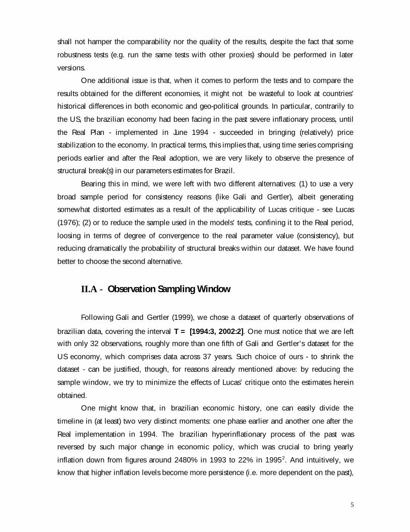
(ii): st – Marginal cost is obtained from the following expression:

st = log[St] – log[S*t],

where St = (WtNt)/ (GDPt n).

Wt is working people’s income (Rendimento Real das Pessoas Ocupadas –IBGE), Nt is labor

force (Ocupação - IBGE) and NGDPt is nominal gross domestic product (PIB Nominal –

IBGE). So, s(t) represents deviation of labor income share from its steady state value, which

we’ll assume here, as a proxy, to be its long term average. The idea of why one comes to use

such a measure in our tests will be given in Section IV. (See Figure 1)

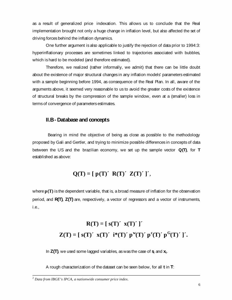
(iii): xt is the detrended output gap:

xt = yt – y*t,

where, yt is the log of output (i.e., the log of the nominal GDP, released by IBGE, and

deflated by FGV’s IGP-M). Meanwhile, yt* is the a long run trend for the real GDP, a proxy

for the natural output, calculated using Hodrick-Prescott’s methodology (HP-Filter). (See

Figure 2)

(iv): it* is interest rates term spread. It is an instrument, which captures the evolution of the

difference between long run and short run interest rates. Such variable is heavily influenced

by future expected inflation. In our tests, we use the difference between TJLP rate (% per

8

annun) and 30 days CDB rate (bank deposit rates), with the first being a proxy for long run

interest rates, and the latter playing the role of short term interests.

(v): πwt and πc

t are, respectively, percent change of labor income (a variable also used to

calculate s(t)) and percent change of FIPE’s IPC index (consumer’s price index). The first plays

the role of wage inflation, whilst the latter is just a standard consumer’s inflation measure.

(vi): π Gt is FGV’s IGP-DI index, another broad inflation measure, which comprises the same

imput variables as IGP-M (with the same weights), differing only in the period of observation

(difference of 10 days). It is used as instrument in most of our tests.

The interested reader will find out that this sample specification is closely connected

to the dataset used by Gali and Gertler, with marginal differences in interpretability, as in the

case of IGP-M substituing a measure like GDP Deflator. Even the choice of the set of

instruments used has respected the standards adopted in Gali and Gertler (1999).

II.C – Econometric Issues

As is commonly done across the literature, when it comes to estimate rational

expectation models, we test models using the generalized method of moments (GMM),

which also follows Gali and Gertler’s way. We shall estimate, for each model, both the

reduced and structural forms (when possible), sometimes imposing restrictions in some

parameters, in order to assess the robustness of results encountered, just like the original

authors have done.

The set of instruments utilized in GMM estimation will be the same for all tests

conduced throughout this work. In this regard, the only diverging point from the original

article is that we used up to 3 lags of each instruments, against 4 in Gali and Gerler (1999).

This was motivated by problem we faced with lack of data - contrarily to what happened in

the american research’s case - for the more lags we use, the less observations we have to

estimate models’ parameters. Comfortably, following that methodological decision, one

should expect no significant effect whatsoever in terms of parameters estimates, and results’

comparability. The set of instruments used is constituted by: lag 3 of wage inflation; lag 3 of

IPC; lag 2 of interest rate term spread; lag 2 of the output gap (HP-Filter); lags 0 until 3 of

IGP-DI and, finally, lags 1 and 2 of marginal cost.

9

For every model estimated, we used Heteroskedastic Autoregressive Consistent (HAC)

Covariance Matrix, proposed by Newey & West (1987), which guarantees more precise

standard error estimates, which are robust to both heteroskedasticity and serial correlation.

This allows us to be more confident on the results generated by the t-statistics, which will be

rejecting (or accepting) the null that the parameter equal zero with greater precision than

otherwise.

In case of models estimated by GMM (the vast majority in this work), we will perform

tests on the overidentifying restrictions, the so called TJ test. Unwilling to go so much deep

into econometric details, for this is not the scope here, the TJ statistic provide a test on the

null hypothesis that the excessive number of moments condition (i.e. the number of

instruments that exceeds the quantity of parameters estimated into the estimated equation) are

indeed valid. One can prove that TJ statistic is distributed by a Chi-Square p.d.f., with

w = r - a degrees of freedom, where r is the number of instruments and a the number of

parameters to be estimated. More details on such test can be found in Hamilton (1994).

III. The Problem of Estimating NKPC Using Output Gap

III.A – Some Theory First

One arrives at the NKPC by solving the problem of a monopolistically competitive

firm (or set of identical firms), which sets its (their) prices optimally, i.e., determining them

such that profits are maximized, subject to the constraint of time-dependent price adjustment.

Accordingly to Calvo, from the hypothesis of constant price elasticity of demand, we

obtain an aggregate price level such as follows (pt is the log of price level, which for

simplicity we name just price level):

pt = θpt-1 + (1-θ) pt* (1),

where θ is the probability that a firm will not change its prices in the current period. So,

aggregate price level is a convex combination of last period’s price level and an optimal price

set by firms (those able to change price in the current period).

10

Letting mct represents the deviation of a firm’s real marginal costs from its steady

state, and β the subjective discount rate, firms maximize their expected discounted profits (by

an stochastic discount factor, which adjusts for the risk), subject to time-dependent price

rules, determining their prices according to the expression below, for k between zero and

infinity:

pt* = (1-θ) Σk(βθ)kEt{mct+k} (2).

It is interesting to notice that, when θ = 0, we have the case of fully flexible prices,

which in such case is to move accordingly to current marginal costs dynamics.

Letting π t = pt – pt-1 denote the inflation rate in tth period, the two expressions above

lead us to the following testable equation (for apropriate mct):

πt = λmct + βEt{π t+1} (3),

where λ = θ-1 (1 - θ) (1 - βθ).

Using lead operators, we obtain, for k between zero and infinity:

πt = λ ΣkβkEt{mct+k} (4).

III.B – The econometrics of the NKPC (Traditional Approach)

In the past, researchers used the following relation to estimate expression (3):

mct = κxt (5),

where xt = yt – yt*, being yt the log of the product, and yt* the log of the “natural” product,

econometrically obtained through some smoothing methodology. Such hypothesis of linear

11

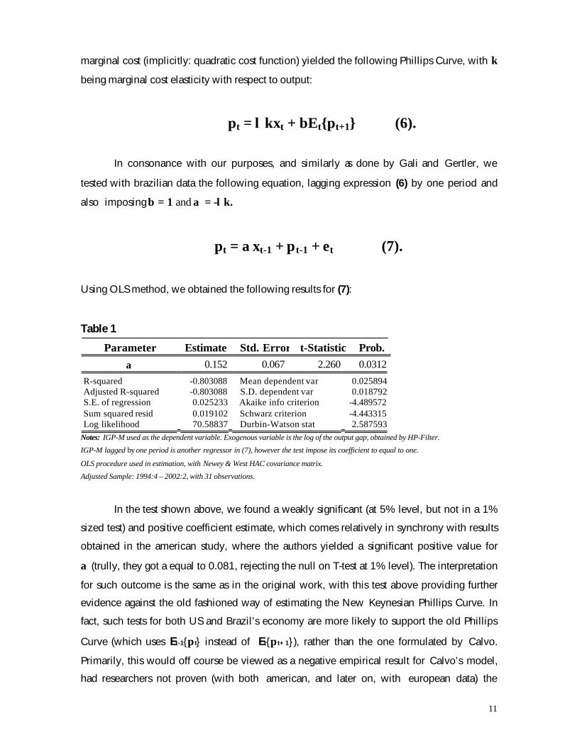
marginal cost (implicitly: quadratic cost function) yielded the following Phillips Curve, with κ

being marginal cost elasticity with respect to output:

πt = λκxt + βEt{πt+1} (6).

In consonance with our purposes, and similarly as done by Gali and Gertler, we

tested with brazilian data the following equation, lagging expression (6) by one period and

also imposing β = 1 and α = -λk.

πt = αxt-1 + π t-1 + εt (7).

Using OLS method, we obtained the following results for (7):

Table 1

Parameter Estimate Std. Error t-Statistic Prob.α 0.152 0.067 2.260 0.0312

R-squared -0.803088 Mean dependent var 0.025894Adjusted R-squared -0.803088 S.D. dependent var 0.018792S.E. of regression 0.025233 Akaike info criterion -4.489572Sum squared resid 0.019102 Schwarz criterion -4.443315Log likelihood 70.58837 Durbin-Watson stat 2.587593

Notes: IGP-M used as the dependent variable. Exogenous variable is the log of the output gap, obtained by HP-Filter.

IGP-M lagged by one period is another regressor in (7), however the test impose its coefficient to equal to one.

OLS procedure used in estimation, with Newey & West HAC covariance matrix.

Adjusted Sample: 1994:4 – 2002:2, with 31 observations.

In the test shown above, we found a weakly significant (at 5% level, but not in a 1%

sized test) and positive coefficient estimate, which comes relatively in synchrony with results

obtained in the american study, where the authors yielded a significant positive value for

α (trully, they got a equal to 0.081, rejecting the null on T-test at 1% level). The interpretation

for such outcome is the same as in the original work, with this test above providing further

evidence against the old fashioned way of estimating the New Keynesian Phillips Curve. In

fact, such tests for both US and Brazil’s economy are more likely to support the old Phillips

Curve (which uses Et-1{π t} instead of Et{π t+1}), rather than the one formulated by Calvo.

Primarily, this would off course be viewed as a negative empirical result for Calvo’s model,

had researchers not proven (with both american, and later on, with european data) the

12

validity of the marginal cost approach to estimate parameters from the NKPC in Calvo’s

fashion. We shall verify, in the sections that follow, if such results also hold true for the

brazilian economy as well.

IV. Marginal Costs Approach: The Purely Forward

Looking NKPC

IV.A – Motivating The New Specification

The poor empirical results obtained by Calvo’s NKPC, using data from both US and

Brazil’s economy (the latter testified by the earlier section of this current work), when

computing the output gap by some smooth technique, might not be a decisive evidence

against Calvo’s model. In other words, these bad results should not lead to the rejection of its

empirical validity, as some might conclude at a first glance. Gali and Gartler’s point is that

such results are directly influenced by the methodology used to obtain the natural output, and

the outcome of empirical tests on NKPC may be quite different conditional on the smoothing

technique deployed. The authors claim that structural shocks, like change in tastes and

variations in government spending may have an impact such that it offsets the forecasted

negative relation between inflation acceleration today and the output gap last period. So it

would be useful if we had a proxy for the output gap which did not suffer from this problem.

The approach used here (for brazilian data), originally proposed in Gali and Gertler (1999), is

to use marginal costs as a proxy to the output gap.

Gali and Gertler sustain that an alternative way to test the NKPC model is, instead of

estimating equation (6), estimating the expression (3), replacing therefore the output gap (xt)

by the marginal costs (mct). Since the latter are not directly observable, we must use theory to

guide efforts on how to obtain such variable, so allowing us to go into estimation procedures.

Section II.B of this current work shows details on how we obtained the measure of marginal

costs (for the brazilian economy) which is deployed here. It is important to highlight here that

the procedure used to get the marginal costs measure is meant to be as near as possible to the

one proposed by the authors in this paper’s “original (american) version”.

Let’s go straight to the point, now. Suppose a Cobb Douglas production function like

13

Yt = AtKtαkNt

αn (8).

Real marginal costs can be expressed by the ratio of the real wage to the labor’s

marginal product:

MCt = (Wt/Pt)( ? Yt/? Nt)-1 (9).

Some algebraic manipulations, i.e., inserting using expression (8) and the partial

derivative of Yt with respect to Nt into (9), yields the following expression below:

MCt = Stαn-1 (10),

where St = WtNt(PtYt)-1.

From St, the share of labor income, we obtain st, which represents the percent

deviations of St from its steady state level (the latter is estimated by use of HP-Filter):

st = log[St] – log[St*] (10*).

Then, st will then be used in the NKPC’s specifications that we test here, providing

our measure of marginal cost that will replace (as a proxy for) the standard measure of the

output gap.

So, in the next section, we test the following version of Calvo’s NKPC:

πt = λ st + βEt{πt+1} (11),

where λ = θ-1 (1 - θ) (1 - βθ).

14

IV.B – Testing Calvo’s NKPC Using Marginal Costs

IV.B.1 – Reduced Form Estimates

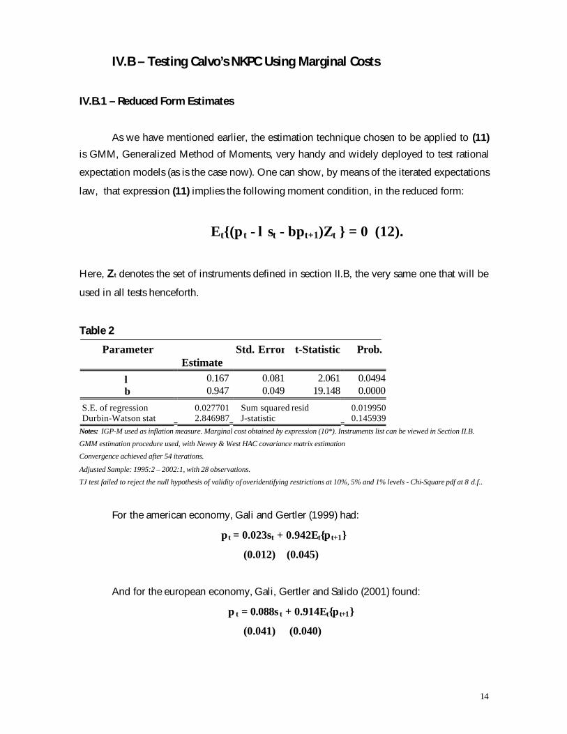
As we have mentioned earlier, the estimation technique chosen to be applied to (11)

is GMM, Generalized Method of Moments, very handy and widely deployed to test rational

expectation models (as is the case now). One can show, by means of the iterated expectations

law, that expression (11) implies the following moment condition, in the reduced form:

Et{(π t - λ st - βπt+1)Zt } = 0 (12).

Here, Zt denotes the set of instruments defined in section II.B, the very same one that will be

used in all tests henceforth.

Table 2

ParameterEstimate

Std. Error t-Statistic Prob.

λ 0.167 0.081 2.061 0.0494β 0.947 0.049 19.148 0.0000

S.E. of regression 0.027701 Sum squared resid 0.019950Durbin-Watson stat 2.846987 J-statistic 0.145939

Notes: IGP-M used as inflation measure. Marginal cost obtained by expression (10*). Instruments list can be viewed in Section II.B.

GMM estimation procedure used, with Newey & West HAC covariance matrix estimation

Convergence achieved after 54 iterations.


TJ test failed to reject the null hypothesis of validity of overidentifying restrictions at 10%, 5% and 1% levels - Chi-Square pdf at 8 d.f..

For the american economy, Gali and Gertler (1999) had:

π t = 0.023st + 0.942Et{π t+1}

(0.012) (0.045)

And for the european economy, Gali, Gertler and Salido (2001) found:

π t = 0.088s t + 0.914Et{π t+1}

(0.041) (0.040)

15

Thus, what we got a positive (and significant at 5%) value for λ, using marginal cost

replacing as a proxy to the “actual” output gap. These results exposed in the table above are

not so different to those obtained for the american economy (listed below). The great

discrepancy concerns the estimates for λ, given that output elasticity obtained for brazilian

data is 7 times as high as the one gotten in the american case, and almost the double of

estimates from european economy. In addition, the significance of λ is rather weak in

brazilian case, for we fail to reject the null at 1% level, contrarily to what happens for the

Europe and US economies. Nevertheless, it is also interesting to notice the similar values

obtained for the betas (not only coefficient estimates, but also standard deviations), implying

impatience rates relatively consistent, and not very contradictory, across the three economies

tested.

It could also be worthwhile to provide, at this point, some information on the TJ test.

In the test of (12), we failed to reject the null hypothesis about the validity of the (r – a)

overidentifying restrictions, where r is the quantity of instruments (10) and a is the number of

parameters estimated (2). At 5%, the critical value of Chi-Square at 8 degrees of freedom is

15.51, greater than the value of 4.09 obtained for the TJ statistic. In fact, the same will

happen to all conditions tested henceforth, so we shall not waste time in detailing further TJ

results on these tests.

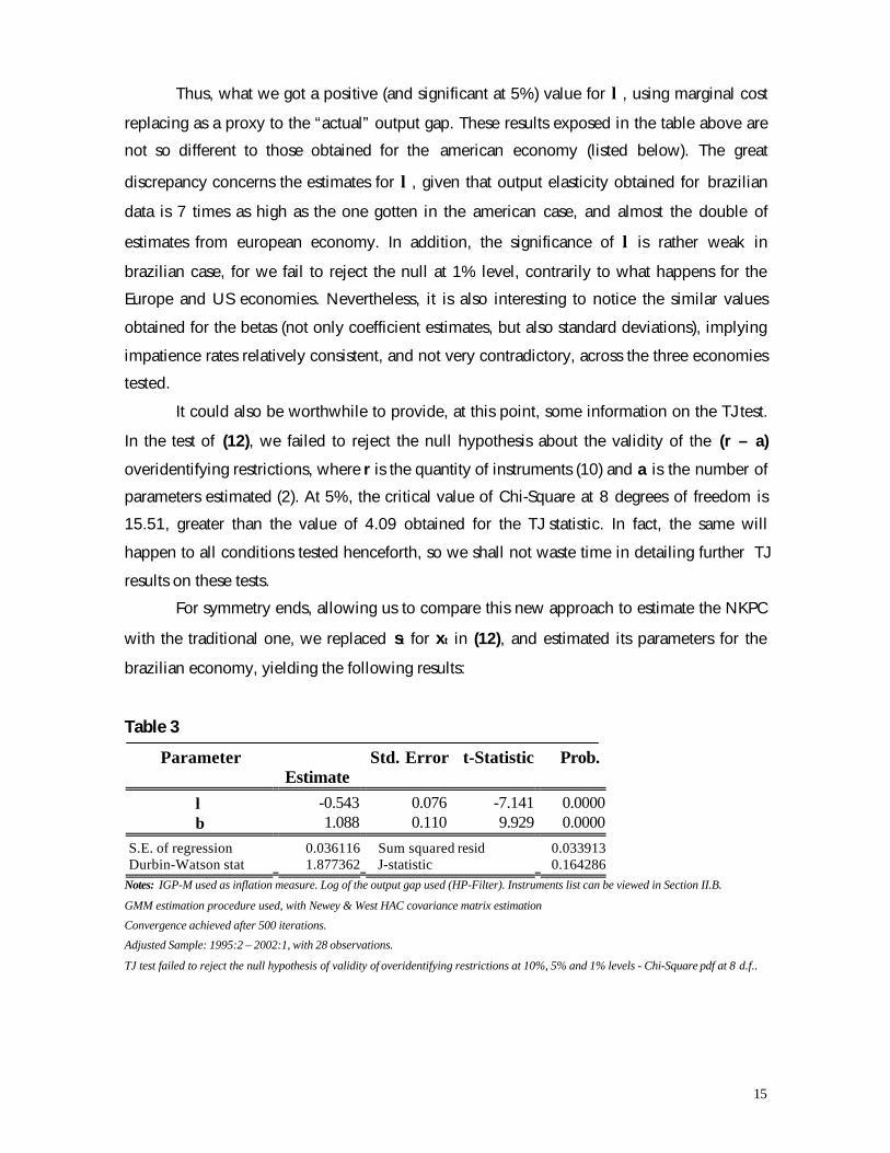
For symmetry ends, allowing us to compare this new approach to estimate the NKPC

with the traditional one, we replaced st for xt in (12), and estimated its parameters for the

brazilian economy, yielding the following results:

Table 3

ParameterEstimate

Std. Error t-Statistic Prob.

λ -0.543 0.076 -7.141 0.0000β 1.088 0.110 9.929 0.0000


Notes: IGP-M used as inflation measure. Log of the output gap used (HP-Filter). Instruments list can be viewed in Section II.B.





16

With regard to this particular test, results for the US economy were3:

π t = -0.016xt + 0.988Et{π t+1}

(0.005) (0.030)

For Europe, it was found that:

π t = -0.003xt + 0.990Et{π t+1}

(0.007) (0.018)

Although our test above has come up with an estimate for λ differing considerably

from those obtained in Gali and Gertler (1999) for american data, and in Gali, Gertler and

Salido (2001) for european data, in general, the evidence found here is roughly the same as in

the papers cited above: results of empirical tests on NKPC have been poorer replacing

marginal costs by conventional output gap measure (i.e. log-output detrended by HP-Filter).

And, at the margin, results encountered for the brazilian sample have become even worse

using the standard output gap, in comparison to the tests performed for the other economies.

To justify this claim, we have the observation here of a negative λ (the same sign as in

the test for US and Europe), as well as the finding of β> 1, similarly as new estmates for the

US economy. Using results from ours and other previous experiments, we robustly find that

results on NKPC estimation, mainly those concerning the sign of parameter λ, depend heavily

on type the instrument chosen to proxy the output gap. Furthermore, the value found for the

beta (yielding an estimate greater than one for both US and Brazil, see footnote 3) is very

implausible, for agents should not like better the future than the present, a widely accepted

economic hypothesis unobserved by a negative impatience rate implied by β> 1. In all, the

tests with brazilian data shown here may strengthen the conclusion that the use of marginal

cost approach is indeed valid to estimate the NKPC. It also reinforce empirical evidence

favoring Calvo’s model.

IV.B.2 – Structural Form Estimates

The tests displayed above were performed using reduced form equations. An

additional exercise useful at this point is try to estimate equation (12) in the structural form,

that is, to test an specification where (in particular) parameter λ is written as function of θ and

β. In case of (12), by the use of (11), we have:

3 In Gali, Gertler and Salido (2001), they show new ( updated)estimates for the american economy, where it

17

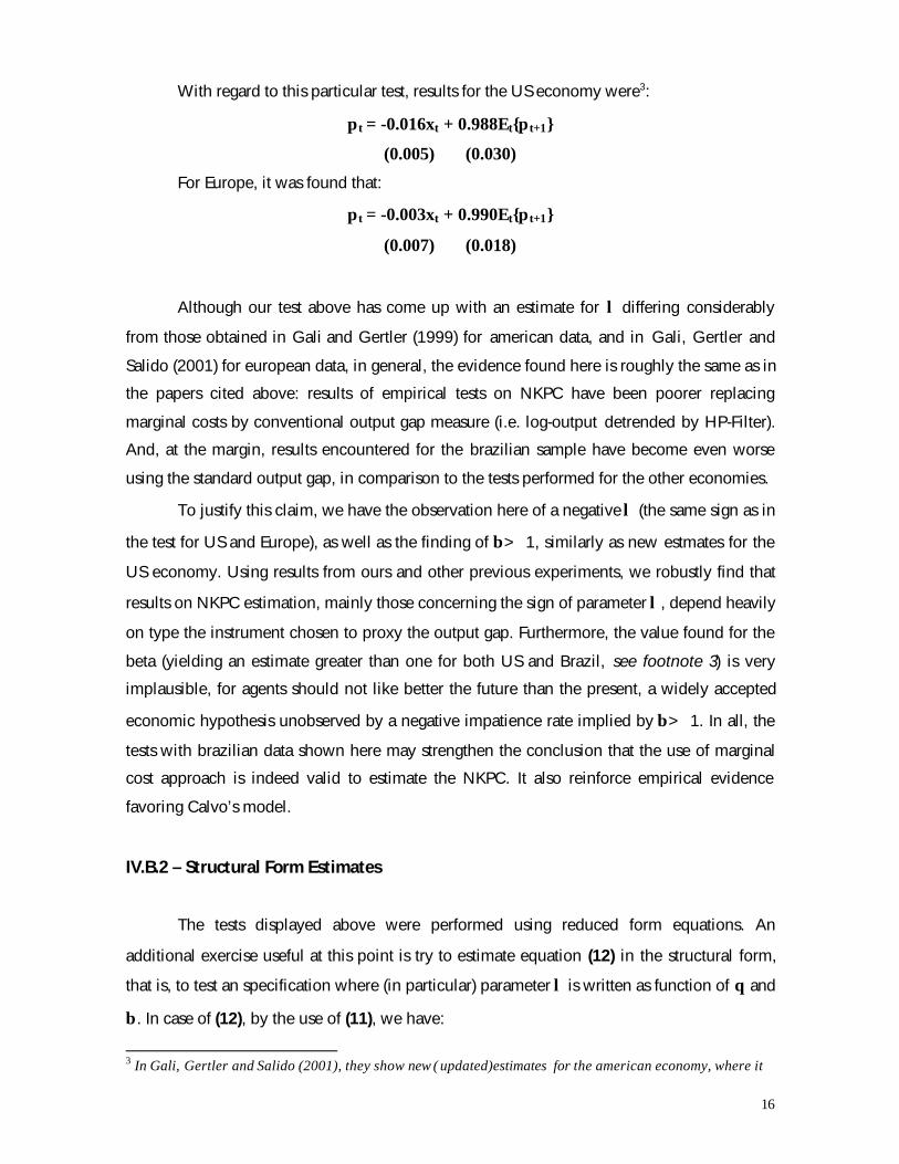
Et{(θπt – (1-θ)(1-θβ)st – θβπ t+1)Zt} = 0 (13).

So, our next step is to estimate equation (13), using exactly the same set of

instruments used before, which will now allow us to obtain estimates for the structural

parameter θ. The importance of such parameter is that, in Calvo’s model, it denotes the

probability that a given price setter will leave price unchanged in the current period. With

knowledge of this parameters, one is able to determine the average time that a certain price is

to remain unchanged, which is given by:

(1-θ)Σkkθk-1 = (1-θ)-1 (E).

More details on that can be found in Gali and Gertler (1999b). By use of this

expression above, we find an interesting empirical measure: how often, in average, agents

change their prices. In a comparative basis across countries, we expect the brazilian data to

show agents changing prices more frequently than in US and Europe, regions where inflation

has let few “scars” in the recent decades.

Tests performed on equation (13) gave us the following results:

Table 4

ParameterEstimate

Std.Error

t-Statistic Prob.

θ 0.593 0.035 16.705 0.0000β 0.875 0.052 16.814 0.0000λa 0.330 - - -






TJ test failed to reject the null hypothesis of validity of overidentifying restrictions at 10%, 5% and 1% levels - Chi-Square pdf at 8 d.f..a Implied value for λ obtained by replacing estimated θ and β in expression (11).

turned out that λ = 0.021, and β = 1.012, both significant at 1% level.

18

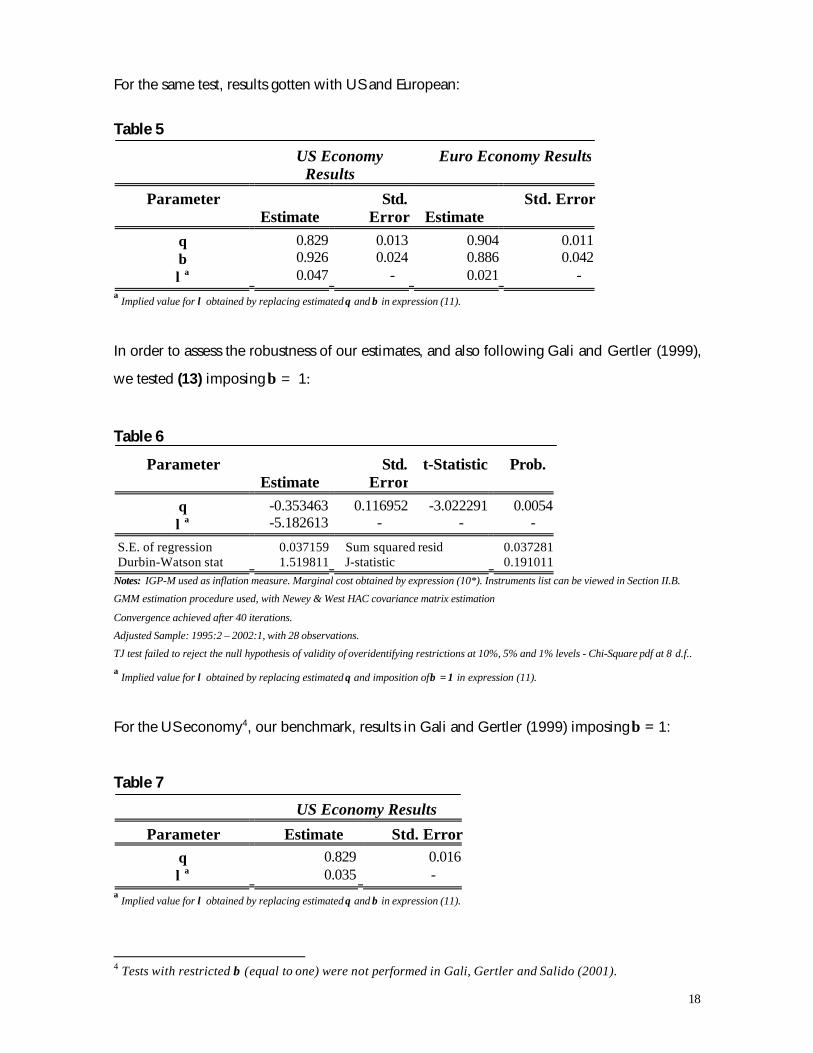
For the same test, results gotten with US and European:

Table 5

US EconomyResults

Euro Economy Results

ParameterEstimate

Std.Error Estimate

Std. Error

θ 0.829 0.013 0.904 0.011β 0.926 0.024 0.886 0.042λa 0.047 - 0.021 -

a Implied value for λ obtained by replacing estimated θ and β in expression (11).

In order to assess the robustness of our estimates, and also following Gali and Gertler (1999),

we tested (13) imposing β = 1:

Table 6

ParameterEstimate

Std.Error

t-Statistic Prob.

θ -0.353463 0.116952 -3.022291 0.0054λa -5.182613 - - -







a Implied value for λ obtained by replacing estimated θ and imposition of β = 1 in expression (11).

For the US economy4, our benchmark, results in Gali and Gertler (1999) imposing β = 1:

Table 7

US Economy Results

Parameter Estimate Std. Errorθ 0.829 0.016λa 0.035 -


4 Tests with restricted β (equal to one) were not performed in Gali, Gertler and Salido (2001).

19

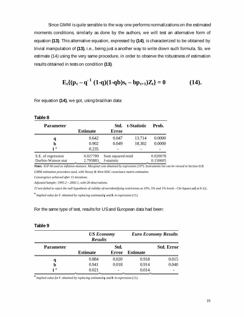
Since GMM is quite sensible to the way one performs normalizations on the estimated

moments conditions, similarly as done by the authors, we will test an alternative form of

equation (13). This alternative equation, expressed by (14), is characterized to be obtained by

trivial manipulation of (13), i.e., being just a another way to write down such formula. So, we

estimate (14) using the very same procedure, in order to observe the robustness of estimation

results obtained in tests on condition (13).

Et{(π t – θ−1 (1-θ)(1-θβ)st – βπ t+1)Zt} = 0 (14).

For equation (14), we got, using brazilian data:

Table 8

ParameterEstimate

Std.Error

t-Statistic Prob.

θ 0.642 0.047 13.714 0.0000β 0.902 0.049 18.302 0.0000λa 0.235 - - -






TJ test failed to reject the null hypothesis of validity of overidentifying restrictions at 10%, 5% and 1% levels - Chi-Square pdf at 8 d.f..a Implied value for λ obtained by replacing estimated θ and β in expression (11).

For the same type of test, results for US and European data had been:

Table 9

US EconomyResults

Euro Economy Results

ParameterEstimate

Std.Error Estimate

Std. Error

θ 0.884 0.020 0.918 0.015β 0.941 0.018 0.914 0.040λa 0.021 - 0.014 -


20

Analogously, imposing β = 1:

Table 10

ParameterEstimate

Std.Error

t-Statistic Prob.

θ 0.699 0.073 9.618 0.0000λa 0.130 - - -








For the US economy5, our benchmark, results in Gali and Gertler (1999) were:

Table 11

US EconomyResults

ParameterEstimate

Std.Error

θ 0.915 0.035λa 0.007 -


It is worthwhile at this time to establish some comments on the results shown above.

In what refers to parameter λ, results robustly indicate a higher estimated value for brazilian

economy (comparing to those gotten from US and Europe), with our estimates ranging in

general on (0.13,0.33). This is an evidence that the output-gap6 elasticity of inflation is greater

for Brazil’s economy, implying that, in this country, inflation responds more (generally

upwards, we know) to given changes in output gap, in comparison to other developed

countries. This is a somewhat intuitive result, for historical reasons, since Brazil has lived

periods of huge inflation, and this may institutionally have affected the way inflation (through

5 Tests with restricted β (equal to one) were not performed in Gali, Gertler and Salido (2001).6 Using marginal costs as a proxy.

21

price setters) responds to output movements, despite the fact that we cannot rule out the

possibility that maybe the difference is to high to be true.

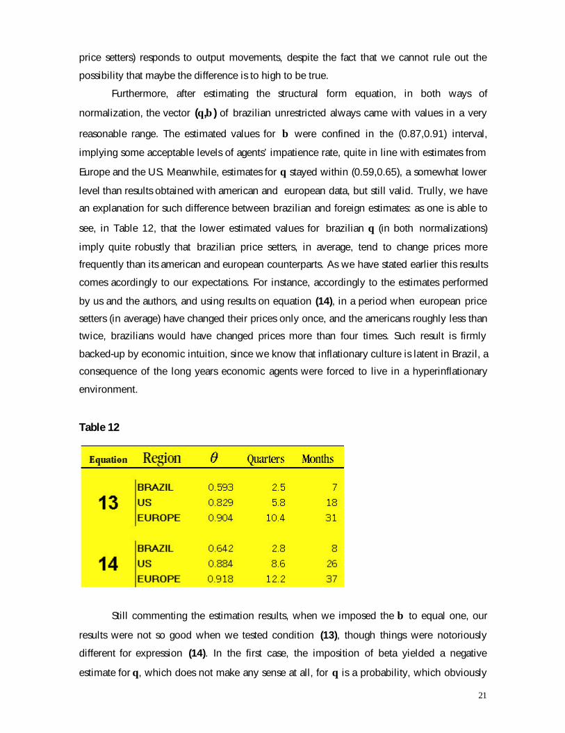
Furthermore, after estimating the structural form equation, in both ways of

normalization, the vector (θ,β ) of brazilian unrestricted always came with values in a very

reasonable range. The estimated values for β were confined in the (0.87,0.91) interval,

implying some acceptable levels of agents’ impatience rate, quite in line with estimates from

Europe and the US. Meanwhile, estimates for θ stayed within (0.59,0.65), a somewhat lower

level than results obtained with american and european data, but still valid. Trully, we have

an explanation for such difference between brazilian and foreign estimates: as one is able to

see, in Table 12, that the lower estimated values for brazilian θ (in both normalizations)

imply quite robustly that brazilian price setters, in average, tend to change prices more

frequently than its american and european counterparts. As we have stated earlier this results

comes acordingly to our expectations. For instance, accordingly to the estimates performed

by us and the authors, and using results on equation (14), in a period when european price

setters (in average) have changed their prices only once, and the americans roughly less than

twice, brazilians would have changed prices more than four times. Such result is firmly

backed-up by economic intuition, since we know that inflationary culture is latent in Brazil, a

consequence of the long years economic agents were forced to live in a hyperinflationary

environment.

Table 12

Still commenting the estimation results, when we imposed the β to equal one, our

results were not so good when we tested condition (13), though things were notoriously

different for expression (14). In the first case, the imposition of beta yielded a negative

estimate for θ, which does not make any sense at all, for θ is a probability, which obviously

22

must lie in the interval [0,1]. In the latter case, however, the estimate for θ was very robust to

the restriction imposed, and the estimates lied within (0.64, 0.70), not much different from

the unrestricted estimate of (13).

The sticky result obtained in (13), which did not resist to the imposition of β =1,

contrasting with american results, proven to be more robust, is indeed something that lead us

to seek explanations. One excuse we have is that is sample size asymmetries between the

two studies (our and Gali and Gertler’s), with the american work having much more data

available - around 37 years of quarterly observations - compared to the 32 quarterly

observations within our dataset. We can speculate that this sets a toll into the robustness of

our results, because of consistency reasons.

Notwithstanding, in the overall, having obtained some reasonable estimates for

parameters in the tests performed here, one should be quite satisfied with the results herein

mentioned. They should, indeed, be considered as another good evidence for Calvo’s

implied NKPC, supporting Gali and Gertler’s argument.

V. Marginal Costs Approach: The Hybrid NKPC

V.A – Motivating The New Specification

As we pointed out earlier, some of the criticism on Calvo’s derivation of the NKPC is

aimed at the purely forward looking agent’s behavior it implies. In fact, NKPC supposes

unrealistically that only current and future events in the economy (more specifically, the ones

affecting the output gap) will be important in inflation determination. Nevertheless, no single

economist, who roughly watches empirical economic events, can feel comfortable with such

an idea. It underestimates the phenomenon of persistence in inflation trajectory, which has

already been documented by empirical work like Christiano et al.(2001).

In addition, most central banks around the world use inflation models incorporating

such feature. In particular, the Central Bank of Brazil is no exception to such rule, with all

versions of its inflation targeting model hypothesizing a variant of Phillips Curve which

allows for the presence of inertia in inflation stochastic process7. With this regard, inflation

inertia in Brazil is considered by economists as key issue for the pathological

hyperinflationary process observed in the country’s economic past.

23

In order to test for the presence of a backward looking component in the inflation

trajectory, we run some models for the Brazilian economy, still in the Gali and Gertler’s

flavor. In their paper, using Calvo’s framework, they attach to the purely forward looking

NKPC a backward looking inflation component, in order to capture the persistence effects in

inflationary process.

V.B – Some Theory, Just for The Record

Respecting the same set of assumptions adopted in Calvo’s model, we might now

suppose, additionally (in ad hoc way), that some fraction ω of firms use an easy rule of thumb

to set their prices, based on past information. This is somewhat different from what we had

before: a bunch (randomly selected) companies setting prices by solving their profit

maximization problem, subject to time-dependent adjustments constraints, using all

information available to foresee future economic conditions, mainly, future marginal costs.

We shall now classify these firms as Forward Looking (FL), henceforth. In addition to these

firms, our new economy has another class of price setters - firms that set prices depending on

what they observed in the past – using history-dependent price rules. They constitute the

group of Backward Looking firms (BL).

In such environment, aggregate prices are determined by the following expressions:

pt = θpt-1 + (1-θ)pt* (15),

pt* = (1-ω)ptf + ωpt

b (16),

where pt* is the restricted aggregate price index, for prices set in the current period, ptf and

ptb are, respectively, new prices for (FL) and (BL) firms. They obey the following rules (let k be

a time-index from period zero to infinity):

ptf = (1-θβ)Σk(θβ)kEt{mct+k} (17),

ptb= p t-1* + π t-1 (18).

7 The interested reader is referred to Bogdanski, Tombini and Werlang (2000) and Bogdanski et al.(2001).

24

One can observe that ptf is just the optimal price chosen in the purely forward looking

model. It is worth to verify that the (ad hoc) establishment of ptb has an interesting property:

for stationary inflation dynamics, the rule converges to the optimal forward looking price

setting rule, as time goes by.

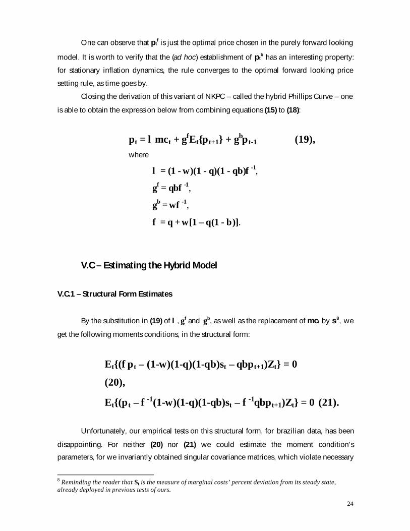
Closing the derivation of this variant of NKPC – called the hybrid Phillips Curve – one

is able to obtain the expression below from combining equations (15) to (18):

πt = λmct + γfEt{π t+1} + γbπ t-1 (19),where

λ = (1 - ω )(1 - θ)(1 - θβ)φ-1,

γf = θβφ -1,

γb = ωφ-1,

φ = θ + ω [1 – θ(1 - β)].

V.C – Estimating the Hybrid Model

V.C.1 – Structural Form Estimates

By the substitution in (19) of λ, γ f and γb, as well as the replacement of mct by st8, we

get the following moments conditions, in the structural form:

Et{(φπt – (1-ω)(1-θ)(1-θβ)st – θβπt+1)Zt} = 0

(20),

Et{(π t – φ-1(1-ω)(1-θ)(1-θβ)st – φ-1θβπt+1)Zt} = 0 (21).

Unfortunately, our empirical tests on this structural form, for brazilian data, has been

disappointing. For neither (20) nor (21) we could estimate the moment condition’s

parameters, for we invariantly obtained singular covariance matrices, which violate necessary

8 Reminding the reader that St is the measure of marginal costs’ percent deviation from its steady state,already deployed in previous tests of ours.

25

boundness condition and impede us to obtain valid estimates. This also happened for other

instrument sets than Zt also tested.

One hypothetical explanation is that micronumerosity is showing its ugly head here,

setting a huge toll on the estimation procedures. Moreover, it is worth highlighting that when

we imposed a restriction that ω = 1, the singular matrix problem could be solved for the set

of instruments deployed throughout this work (i.e. Zt), but this would not resolve our

problem.

In all, this is quite bad for empirical reasons, for it would be useful to have further

estimates that could (luckily) strengthen our conclusions already reached over θ, β and λ,as

well as it could provide (brand new) estimates for ω, γb and γf, parameters for which we have

no results whatsoever this far.

In the paper that inspired this current work, Gali and Gertler have only tested the

structural form equations, and they never mention anything about reduced form estimation

results on the hybrid curve. So, in order to observe empirical evidence on such important

issue - the degree of brazilian inflation’s persistence or, if one will, the ‘backwardness’ of the

inflationary dynamics in Brazil - we detach for a while from the procedures adopted in Gali

and Gertler (1999). From now on, we will be encharged to perform tests on the reduced form

of the hybrid NKPC.

V.C.1 – Reduced Form Estimates

As just stated above, in this sub-section, with will to obtain estimates for important

inflation dynamics’ parameters, we mean to test the reduced form of the hybrid curve. In

order to do so, and likewise the procedure followed in the previous tests, we will be using

the marginal costs approach. From expression (19) we get the following testable equation,

substituting mct for our measure of marginal costs percent deviations from its steady-state:

πt = λ st + γfEt{π t+1} + γbπ t-1(22).

Through the application of the Iterated Expectations Law in (22), one obtain the next

moment condition:

Et{(π t – λst – γf πt+1 – γb π t-1)Zt} = 0 (23).

26

Using the same set of instruments as in our previous tests (Zt), the estimation results of (23)

are shown in Table 13:

Table 13

Parameter Estimate Std. Error t-Statistic Prob.λ 0.480 0.088 5.429 0.0000γf -0.140 0.087 -1.608 0.1203γb 0.704 0.083 8.445 0.0000







In order to gain further interpretability, we compare our estimates with results obtained in

Gali and Gertler (1999) for the US economy, and Gali, Gertler and Salido (2001) for the

european economy. One should be cautious at this point here, for these authors have

estimated only the structural form of the hybrid NKPC, which hampers somewhat the

symmetry of the comparison established herein. Nevertheless, it might not completely

invalidate it, so we display the “foreign” results (for both types of normalization) in Table 14

and 15:

Table 14

US Economy ResultsNormalization (20) Normalization (21)

ParameterEstimate

Std.Error Estimate

Std. Error

λ 0.037 - 0.015 -γf 0.682 0.020 0.591 0.016γb 0.252 0.023 0.378 0.020

27

Table 15

European Economy Results

Normalization (20) Normalization (21)Parameter

Estimate Std.

Error Estimate Std. Error

λ 0.018 - 0.006 -γf 0.877 0.045 0.689 0.044γb 0.025 0.127 0.272 0.072

The results obtained this far for the hybrid NKPC in the brazilian economy allows us

to establish the following parallel to the analogous estimates in the US and european

economies. First of all, in the meantime, the λ are still much higher for the brazilian economy

than for our benchmark economies, which comes very much in line to previous estimates for

the same parameter contained in the NKPC specifications tested before (the levels are

proportional too).

Second, as expected for the historical reasons already mentioned, the brazilian

inflationary dynamics was the one with the highest degree of persistence (or inertia, if one

will). This might well be a consequence of a “price indexation culture” present in Brazil: after

many years of high inflation, price setters became used to observe past inflation and reset

their prices likewise. Maybe this culture or habit has not been left aside yet by a considerable

fraction of brazilian price setters, even after the Real Plan implementation (which indeed

stabilized prices). In other words, our view is that the highly persistent inflation dynamics in

Brazil might be result of sluggish agents’ behavior, who got used to living in a widespread

price indexation environment, as was the case for the Brazilian economy in the past.

Third, one bizarre result that we found is the lack of significance in the forward

looking component in brazilian inflation process. This could hint to some the possibility that

brazilian inflation expectations are, even in the Real era, purely adaptative, implying a high

level of irrationality from price setters in Brazil. This last result is very strong, and may force

us to go into further tests in order to validate it.

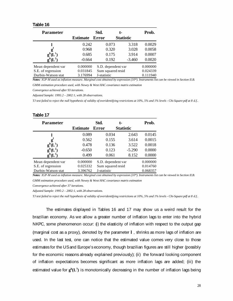
Therefore, for robustness assessment purposes, we also estimated variants of (23)

allowing inflation lags of higher order to enter into the hybrid NKPC specification. The

empirical tests for them in Brazil gave us the following results:

28

Table 16

ParameterEstimate

Std.Error

t-Statistic

Prob.

λ 0.242 0.073 3.318 0.0029γf 0.968 0.320 3.028 0.0058

γb(L1) 0.685 0.175 3.914 0.0007γb(L2) -0.664 0.192 -3.460 0.0020

Mean dependent var 0.000000 S.D. dependent var 0.000000S.E. of regression 0.031845 Sum squared resid 0.024339Durbin-Watson stat 3.176994 J-statistic 0.111940






Table 17

ParameterEstimate

Std.Error

t-Statistic

Prob.

λ 0.089 0.034 2.643 0.0145γf 0.562 0.155 3.614 0.0015

γb(L1) 0.478 0.136 3.522 0.0018γb(L2) -0.650 0.123 -5.290 0.0000γb(L3) 0.499 0.061 8.152 0.0000

Mean dependent var 0.000000 S.D. dependent var 0.000000S.E. of regression 0.025332 Sum squared resid 0.014760Durbin-Watson stat 3.396762 J-statistic 0.068357






The estimates displayed in Tables 16 and 17 may show us a weird result for the

brazilian economy. As we allow a greater number of inflation lags to enter into the hybrid

NKPC, some phenomenon occur: (i) the elasticity of inflation with respect to the output gap

(marginal cost as a proxy), denoted by the parameter λ, shrinks as more lags of inflation are

used. In the last test, one can notice that the estimated value comes very close to those

estimates for the US and Europe’s economy, though brazilian figures are still higher (possibly

for the economic reasons already explained previously); (ii) the forward looking component

of inflation expectations becomes significant as more inflation lags are added; (iii) the

estimated value for γb(L1) is monotonically decreasing in the number of inflation lags being

29

inserted into the hybrid NKPC. Perhaps all issues from (i) to (iii) are a symptom of some

excluded variable bias in coefficient estimates. This is even more clear in case of (iii), when it

seems that γb(L1) gives back the due credit merited by γb(L3) on pushing the current inflation

movements, when the latter is included in the specification.

Anyway, in the last estimation of (23) performed (which includes three inflation lags)

the reasonable estimate for some parameters like λ and γf, which come not only in line with

previous brazilian estimates (in other models) but also compatible to international estimated

values, may be interpreted as a strong hint that this may be the a nice specification to

approximate (i.e. to fit the data on) brazilian inflation dynamics.

Another curious result, and quite robust, we might say, is the negative impact that

inflation lagged by two periods has in current inflation, yielding values close to –0.65 in the

two last tests. This result lacks intuitiveness. The only explanation found this far for this

implied sinusoidal inflation dynamics in Brazil is the possibility that brazilian inflation (in the

Real era) displays a mean-revertion property, which impedes it to diverge. However, we shall

be conservative now and treat this issue more like a puzzle to be resolved, instead of being

satisfied with such explanation (speculation) just given.

One last (but not least) point refers to inflation persistence. As our tests could show as

empirical evidence, brazilian inflation displays huge degree of inertia in prices acceleration.

Such results comes much in line with our expectations based on theory and empirical

literature. This is a quite important issue for policy makers, since at the margin, monetary

policy tends to be less effective in controlling inflation when agents actions are so much

dependent on the past. Or equivalently, such high degree of irrationality may worsen the so

called (and theoretically supported) by Mankiw (2000) “inexorable” tradeoff between

inflation and output.

30

VI. Conclusions

In general, the results obtained in this replication of Gali and Gertler’s experiments,

for the Brazilian economy, were supportive for Calvo´s theory when tests were performed

using real marginal costs as proxy for the true output gap, as was done by the authors. This

outcome comes in line with those obtained for the both US and european economy, despite

some natural differences in estimated parameters. Here, in most tests, we had reasonable

parameter values (i.e. estimates lying in a very acceptable range, accordingly to the theory).

Considering data deficiencies in Brazil, this is something positive.

On empirical grounds, one key conclusion we could obtain with our tests is the deep

and notorious inflationary culture, which is present in Brazil’s economy. Our tests verified

that not only inflationary inertia is a key issue in this country, much more than in the US and

Europe, but also that brazilian price setters, compared to their american and european

counterpart have (in average) habit to change prices much more frequently. In Brazil, one can

say that this is a quite “inflationary” habit, given empirical resistance from price setters to

lower their prices. Another evidence of an inflationary culture is the greater sensibility of

brazilian inflation to the output gap, when compared to the inflation dynamics in both the US

and in Europe. Such conclusion is intuitive, since, in the recent decades, Brazil has suffered

from hyperinflationary maladies, contrarily to what happened for the two other regions

tested.

Notwithstanding, methodologically, one should not disguise the fact that this work

here still needs to be improved in terms of robustness of the results. Some of the parameters

estimated, in spite of being in reasonable parameter range, are still varying undesirably. In

some tests, results changed more than we wanted it to by altering the normalization of

moment’s condition or imposing parameters restrictions.

Robustness is, in fact, the main point that need development in this work. Our guess

is that the smaller degree of robustness in our estimates is caused by the lack of observations

we had (32 points, compared to more than 140 in the american work). In addition to have

hampered any robustness analysis to be performed in sub-periods, the lack of data might have

affected some estimates (the ones showing counter-intuitive results), for parameter estimates’

consistency require greater number of observations. This may explain, also, in our opinion,

the variability of estimates results, because GMM is only asymptotically efficient, and

micronumerosity might have set a toll on variance estimates as well.

31

References

Bogdanski, J., Tombini, A.A., Werlang, S.R.C., 2000, “Implementing Inflation

Targeting in Brazil”, Central Bank of Brazil Working Paper #1.

Bogdanski, J., Freitas, P.S., Goldfajn, I., Tombini, A.A., 2001, “Inflation Targeting in

Brazil: Shocks, Backward-Looking Prices and IMF Conditionality”, Central

Bank of Brazil Working Paper #24, August.

Christiano, L., Eichenbaum, M., Evans, C., 2000, “Monetary Policy Shocks: What Have

We Learned and To What End?”, Handbook of Macroeconomics.

Clarida, R., Gali, J. and Gertler, M., 1999b, “The Science of Monetary Policy: a New

Keynesian Perspective”, Journal of Economic Literature 37 #2, 1661-1707.

Gali, J., 1999, “Technology, Employment, and the Business Cycle: Do

Technology Shocks Explain Aggregate Fluctuations?”, American Economic

Review, March, 249-271.

Gali, J. and Gertler, M., 1999, “Inflation Dynamics: A Structural Econometric

Analysis”, Journal of Monetary Economics 44, 195-222.

Gali, J. and Gertler, M., Salido, J.D.L., 2001, “European Inflation Dynamics”, NBER

Working Paper # 8218.

Hamilton, J.D., 1994, “Time Series Analysis”, Princeton University Press.

Lucas, R.E., 1976, “Econometric Policy Evaluation: A Critique”, Carnegie-

Rochester Conference Series on Public Policy. (1), 19-46.

32

Mankiw, N.G., 2000, “The Inexorable and Mysterious Tradeoff Between

Inflation and Unemployment”, NBER Working Paper # 7884.

Newey, W.K., West, K.D., 1987, “A Simple Positive Semi-Definite

Heteroskedasticity and Autocorrelation Covariance Matrix”, Econometrica (55),

703-708.

Roberts, J.M., 1995, “New Keynesian Economics and the Phillips Curve”, Journal

of Money, Credit and Banking Vol. 27 (4), 975-984.

Sbordone, A.M., 2000, “Prices and Unit Labor Costs: A New Test of Price

Stickiness”, Institute of International Economic Studies, Stockholm, Seminar Paper

#653, April (revised).

Woodford, M., 2001, “Interest and Prices”, mimeo.

33

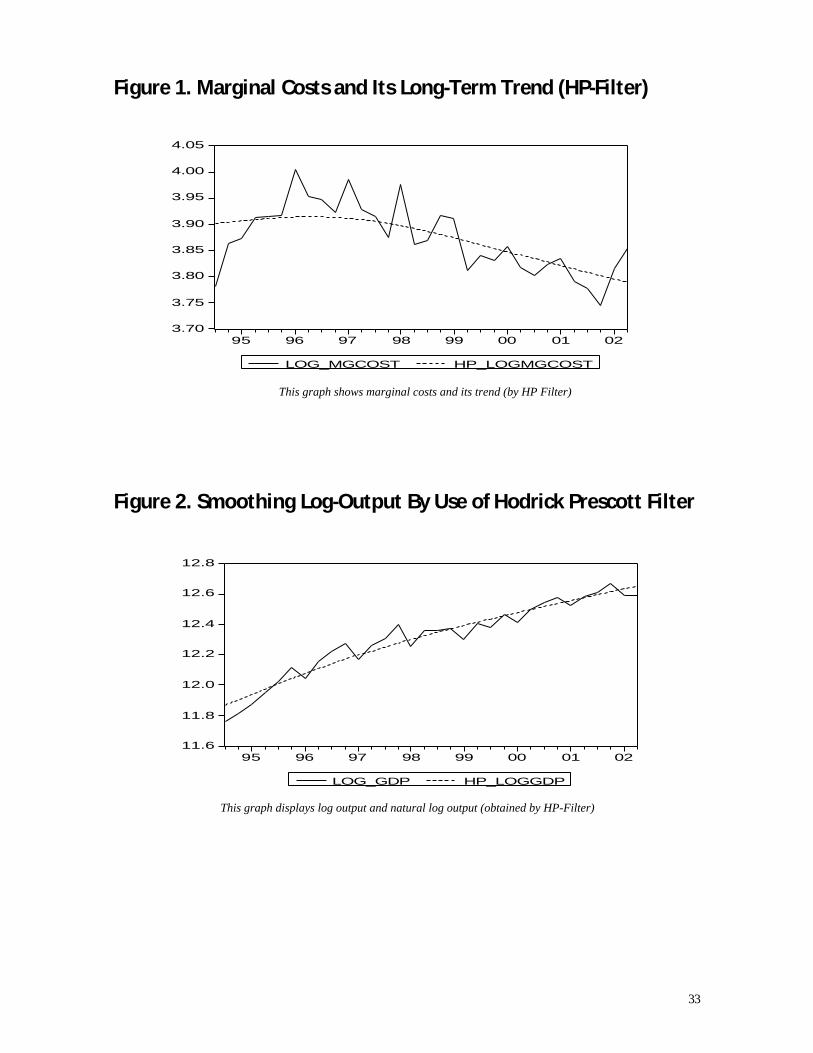
Figure 1. Marginal Costs and Its Long-Term Trend (HP-Filter)

This graph shows marginal costs and its trend (by HP Filter)

Figure 2. Smoothing Log-Output By Use of Hodrick Prescott Filter

This graph displays log output and natural log output (obtained by HP-Filter)

3.70

3.75

3.80

3.85

3.90

3.95

4.00

4.05

95 96 97 98 99 00 01 02

LOG_MGCOST HP_LOGMGCOST

11.6

11.8

12.0

12.2

12.4

12.6

12.8

95 96 97 98 99 00 01 02

LOG_GDP HP_LOGGDP

inflation dynamics in brazil (m.oreng, 2003)

Documents