Inflation Expectations andConsumption Expenditure∗

Francesco D’Acunto,†Daniel Hoang,‡and Michael Weber§

This version: November 2015

AbstractHouseholds that expect an increase in inflation have an 8% higher reported readinessto spend on durables compared to other households. This positive cross-sectionalassociation is stronger for more educated, working-age, high-income, and urbanhouseholds. We document these novel facts using German micro data for the period2000-2013. We use a natural experiment for identification. The German governmentunexpectedly announced in November 2005 a three-percentage-point increase invalue-added tax (VAT) effective in 2007. This shock increased households’inflation expectations during 2006, as well as actual inflation in 2007. Matchedhouseholds in other European countries, which were not exposed to the VAT shock,serve as counterfactuals in a difference-in-differences identification design. Ourfindings suggest fiscal and monetary policy measures that engineer higher inflationexpectations may succeed in stimulating consumption expenditure.

JEL classification: D12, D84, D91, E21, E31, E32, E52, E65

Keywords: Durable Consumption, Zero Lower Bound, Fiscal and Mon-etary Policy, Survey Data, Natural Experiments in Macroeconomics.

∗This research was conducted with restricted access to Gesellschaft fuer Konsumforschung(GfK) data. The views expressed here are those of the authors and do not necessarily reflectthe views of GfK. We thank the project coordinator at GfK, Rolf Buerkl, for help with thedata and insightful comments. We also thank Rudi Bachmann, David Berger, Carola Binder,Jeff Campbell, David Cashin, Robert Chirinko, John Cochrane, George Constantinides, GeneFama, Yuriy Gorodnichenko, Gary Gorton, Anne Hannusch, Tarek Hassan, Jean-Paul L’Huillier,Erik Hurst, Emi Nakamura, Andy Neuhierl, Andreas Neus, Ali Ozdagli, Jonathan Parker, LubosPastor, Carolin Pflueger, Christian Speck, Amir Sufi, Thomas Roende, Martin Ruckes, MayaShaton, Joe Vavra, Johannes Wieland, and seminar participants at the Atlanta Fed, Banque deFrance, Bank of Italy, UC Berkeley, Bocconi, Bundesbank, Cambridge, Chicago, the ChicagoJunior Macro and Finance Meetings, 2015 CITE Conference: New Quantitative Models ofFinancial Markets, the Cleveland Fed Conference on Household Financial Decision Making, EEA2015, EIEF, Federal Reserve Board, 8th joint French Macro Workshop, the 5th meeting of theMacro-Finance Society, NBER ME 2015, SED 2015, and Yale for valuable comments. Webergratefully acknowledges financial support from the University of Chicago, the Neubauer FamilyFoundation, and the Fama–Miller Center.†Haas School of Business, University of California at Berkeley, Berkeley, CA, USA. e-Mail:

francesco dacunto@haas.berkeley.edu‡Department for Finance and Banking, Karlsruhe Institute of Technology, Karlsruhe, B-W,

Germany. e-Mail: daniel.hoang@kit.edu.§Booth School of Business, University of Chicago, Chicago, IL, USA. Corresponding author.

e-Mail: michael.weber@chicagobooth.edu.

I Introduction

Do households act on their inflation expectations? The zero-lower-bound constraint on

conventional monetary policy has revived this question, which is at the center of all New

Keynesian models. Temporarily higher inflation expectations might increase aggregate

demand, stimulate GDP, and bring the economy back to its steady-state growth path.

This argument hinges on two premises: in times of fixed nominal interest rates, higher

inflation expectations decrease real interest rates (Fisher equation), and lower real interest

rates reduce savings and stimulate consumption (Euler equation).1 However, the effect

of real interest rates on consumption depends on assumptions regarding preferences. In

addition, households use paper money as a medium of exchange. Higher inflation is an

implicit tax on paper money, and could lower economic activity.2 Higher inflation might

also increase inflation uncertainty, and reduce consumption spending via a precautionary-

savings channel.3 Ultimately, the sign of the association between households’ inflation

expectations and their willingness to spend on consumption goods is an empirical question.

In this paper, we use German micro data to study the cross-sectional relationship

between inflation expectations and households’ readiness to spend on durable consumption

goods. The market research firm GfK surveys households on a monthly basis to measure

expectations about business-cycle conditions and inflation on behalf of the European

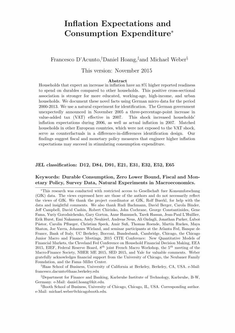
Commission. Figure 1 shows our main finding in a scatter plot for a period from

January 2000 until December 2013. The figure plots the average monthly willingness

to purchase durable goods across surveyed households, against the share of households

that expect inflation to increase in the following 12 months. The solid line is the slope of a

regression of the average willingness to purchase durable goods on our measure of inflation

expectations.4 A positive correlation of 0.59 is present between inflation expectations and

the readiness to spend on durable goods.

The size of this correlation is stable and statistically different from zero throughout

the sample period. The association between inflation expectations and willingness to

purchase durable goods is more pronounced during 2006 (blue points). We discuss this

1Higher inflation expectations may also boost consumption spending through a wealth-redistributionchannel, if borrowers have higher marginal propensities to consume out of wealth (Doepke and Schneider(2006) and Mian, Rao, and Sufi (2013)).

2See Aruoba and Schorfheide (2011).3See Taylor (2013), Bloom (2009), and Pastor and Veronesi (2013).4We describe the data and the construction of our variables in detail in Section II.

1

subperiod in detail below.

Figure 1: Readiness to spend on durables and inflation expectations

2005m11

2005m12

2006m1

2006m2

2006m3

2006m4

2006m52006m6

2006m7

2006m8

2006m9 2006m10

2006m11

2006m12

1.6

1.8

22.

22.

4G

ood

time

to b

uy D

urab

les

0 .1 .2 .3 .4 .5Fraction inflation increases

This figure plots the average monthly readiness to purchase durables on the y-axis against the average

monthly inflation expectation. We use the confidential micro data underlying the GfK Consumer

Climate MAXX survey to construct these variables. GfK asks a representative sample of 2,000

households whether it is a good time to purchase durables given the current economic conditions.

Higher values correspond to better times. GfK also asks how consumer prices will evolve in the next

12 months compared to the previous 12 months. We create a dummy variable that equals 1 when a

household expects inflation to increase. The sample period is January 2000 to December 2013.

In our baseline analysis, we estimate a set of multinomial logit regressions of a

categorical variable that describes the willingness of households to purchase durable

goods on their inflation expectations as well as other household-level characteristics.5

Households that expect higher inflation are on average 8% more likely to report

that it is a good time to buy durable goods, compared to households that expect

constant or decreasing inflation. This positive association holds when we control

for observed household-level heterogeneity with a rich set of demographic variables,

households’ expectations regarding other dimensions such as income or unemployment,

and macroeconomic conditions common to all households. Households expecting higher

5The survey asks households whether it is a good time for them to purchase durable goods givencurrent economic conditions. Households can answer “it is neither a good nor a bad time,” “it is a badtime,” or “it is a good time.” All our results are similar if we interpret the three options as an orderedset of choices, and hence use an ordered probit model for estimation, or if we estimate the relationshipusing ordinary-least squares. See Table A.6 in the online appendix.

2

inflation are also less likely to save, which suggests overall consumption might increase.

We exploit an unexpected, pre-announced value-added tax (VAT) increase as a

natural experiment to assess whether the effect of households’ inflation expectations on

their willingness to purchase durable goods might be causal. Feldstein (2002) suggests

that pre-announced VAT increases can be a discretionary fiscal policy measure to increase

inflation expectations and stimulate private spending.6 Hall and Woodward (2008)

propose temporary sales tax holidays to generate future consumer-goods inflation and

incentivize current spending. Hall (2011) reiterates on this idea in his presidential

address. Correia, Farhi, Nicolini, and Teles (2013) show theoretically that a set of

unconventional fiscal policies, including increasing consumption taxes over time, can fully

offset the zero-lower-bound constraint via stimulating consumer price inflation and achieve

a first-best outcome.

In November 2005, the newly-formed German government unexpectedly announced a

three-percentage-point increase in the VAT effective in January 2007. The administration

legislated the VAT increase to consolidate the federal budget. The increase was unrelated

to prospective economic conditions, and hence it qualifies as an exogenous tax change in

the taxonomy of Romer and Romer (2010). Inflation expectations surged in 2006, and

an increase in realized inflation in 2007 followed. This pattern was unique to Germany

within the European Union.7 The European Central Bank (ECB), which is responsible

for monetary policy and price stability for the whole Euro area, did not increase nominal

rates to offset the higher inflation expectations in Germany. Our natural experiment

therefore provides a setting in which inflation expectations increased while nominal rates

were stable.

We use households in European Union countries not exposed to the VAT shock as

a control group in a difference-in-differences identification strategy. The difference-in-

differences results confirm our baseline findings. To the best of our knowledge, this paper is

the first paper to exploit a natural experiment and a difference-in-differences identification

strategy, to test for the effect of inflation expectations on the readiness to spend.

We also study the heterogeneity of the relationship between inflation expectations

6Feldstein (2002): “This [VAT] tax-induced inflation would give households an incentive to spendsooner rather than waiting until prices are substantially higher.”

7Figure A.2 shows the evolution of inflation expectations for the European Union (EU) and other EUmembership countries.

3

and willingness to spend. The association is higher for household heads with a college

degree, for urban households, for larger households, and for high-income households. The

size of the association is similar across age groups, but it drops by 20% for those in

retirement age.

Two features of the German data make them ideal for studying the relationship

between households’ inflation expectations and their willingness to purchase durable

goods. First, the survey asks households about their willingness to spend on consumption

goods, as opposed to their opinion on whether it is a good time for people in general

to consume, which the Michigan Survey of Consumer (MSC) asks. Second, we can

exploit a natural experiment for identification. This identification setting is close to

the ideal experiment of exogenously increasing households’ inflation expectations in times

of constant nominal interest rates.

Our analysis contains a series of caveats. The survey consists of repeated cross

sections of households. We cannot exploit within-household variation in inflation

expectations to control for time-invariant unobserved heterogeneity at the household

level. The rich set of household demographics, the perception of past inflation, household

expectations regarding their personal economic outlook (e.g., future personal income), and

macroeconomic aggregates (e.g., GDP and unemployment) help alleviate this concern.

Moreover, the survey only elicits a measure of households’ willingness to purchase

consumption goods, and we do not observe the actual consumption behavior of households.

In Figure 11, we show households’ average willingness to spend closely tracks the actual

consumption expenditure on durables. A third potential shortcoming is that the survey

only elicits qualitative measures of inflation expectations. However, evidence suggests

inflation expectations bunch at salient threshold values, and households often report

implausible values for expected inflation rates when asked for quantitative expectations

(see Binder (2015)). Last, pre-announced VAT increases are a salient way to generate

future consumer price inflation and induce current spending. Our baseline findings

continue to hold when we exclude the period after the announcement and before the

effectiveness of the VAT increase. The salience of consumption taxes could be an

advantage of using taxes to engineer negative real interest rates.

Our paper provides empirical support for a growing theoretical literature that

emphasizes the stabilization role of inflation expectations. On the monetary policy side,

4

Krugman (1998), Eggertsson and Woodford (2003), Eggertsson (2006), and Werning

(2012) argue a central bank can stimulate current spending by committing to higher

future inflation rates when the zero lower bound binds. On the fiscal policy side,

Eggertsson (2011), Christiano, Eichenbaum, and Rebelo (2011), Woodford (2011), and

Farhi and Werning (2015) show inflation expectations can increase fiscal multipliers in

standard New Keynesian models in times of a binding zero lower bound. Correia, Farhi,

Nicolini, and Teles (2013) show “unconventional” fiscal policy, including higher future

consumption taxes, can completely offset the zero-lower-bound constraint by generating

consumer price inflation. From a historical perspective, Romer and Romer (2013) argue

deflation expectations caused the Great Depression, whereas Eggertsson (2008) and Jalil

and Rua (2015) suggest a fiscal and monetary policy mix engineered higher inflation

expectations and spurred the recovery from the Great Depression. From an international

perspective, Hausman and Wieland (2014) study the monetary easing of the Bank of Japan

and the expansionary fiscal policy commonly known as “Abenomics.” Their evidence

based on aggregate time series data is consistent with higher inflation expectations raising

consumption and GDP.

We also contribute to the recent literature that uses micro-level data to study

the relationship between inflation expectations and households’ readiness to purchase

consumption goods. Bachmann, Berg, and Sims (2015) start this literature using survey

data from the MSC. They find an economically and statistically insignificant association

between households’ inflation expectations and their readiness to spend on durables.

Burke and Ozdagli (2014) confirm these findings using panel data from the New York

Fed/RAND-American Life Panel household expectations survey for a period from April

2009 to November 2012. Ichiue and Nishiguchi (2015) show Japanese households that

expect higher inflation plan to decrease their future consumption spending.8

We also relate to Cashin and Unayama (2015), who use micro data from the Japanese

Family Income and Expenditure Survey to exploit the VAT increase in Japan to estimate

the intertemporal elasticity of substitution. They do not observe households’ inflation

expectations.

8Other recent papers using inflation expectations data from the MSC are Piazzesi and Schneider(2009), Malmendier and Nagel (2009), Drager and Lamla (2013), Carvalho and Nechio (2014), andCoibion and Gorodnichenko (2012).

5

II Data

A. Data Sources

We use the confidential micro data underlying the GfK Consumer Climate MAXX survey.

GfK conducts the survey on behalf of the Directorate General for Economic and Financial

Affairs (DG ECFIN) of the European Commission.9 GfK monthly asks a representative

repeated cross-section of 2,000 German households questions about general and personal

economic conditions, inflation expectations, and willingness to spend on consumption

goods. We obtained access to the micro data for the period starting in January 2000 and

ending in December 2013. Our sample period includes large variation in macroeconomic

fundamentals, two major recessions, and an unexpected increase in German VAT in 2007.

We use the answers to the following two questions in the survey to construct the

main variables in our baseline analysis:

Question 8 Given the current economic situation, do you think it’s a good time to

buy larger items such as furniture, electronic items, etc.?

Households can answer, “It’s neither a good nor a bad time,” “No, it’s a bad time,” or

“Yes, it’s a good time.”

Question 3 How will consumer prices evolve during the next twelve months compared

to the previous twelve months?

Households can answer, “Prices will increase more,” “Prices will increase by the same,”

“Prices will increase less,” “Prices will stay the same,” or “Prices will decrease.” We

create a dummy variable that equals 1 when households answer, “Prices will increase

more,” to get a measure of higher expected inflation.10

Households’ inflation expectations are highly correlated with their perception of past

inflation (see Jonung (1981)). We also use survey question 2 in our baseline analysis to

disentangle the effects of inflation expectations from inflation perceptions:

Question 2 What is your perception on how consumer prices evolved during the last

twelve months?

9We use similar data from the harmonized surveys of DG ECFIN for several other European countriesin Section IV. We discuss the data in more detail in the online appendix.

10Results do not change if we introduce separate dummies for the individual answer possibilities (seeTable A.5 in the online appendix).

6

Households can answer, “Prices increased substantially,” “Prices increased somewhat,”

“Prices increased slightly,” “Prices remained about the same,” or “Prices decreased.”

The online appendix contains the original survey and a translation to English.

We also use questions regarding expectations about general economic variables,

personal income or unemployment, and a rich set of socio-demographics from the GfK

survey. In robustness checks, we use data on contemporaneous macroeconomic aggregates,

such as GDP and unemployment numbers from the German statistical office (DeStatis),

nominal interest rates, the value of the German stock index DAX, and measures of

European and German policy uncertainty from Baker, Bloom, and Davis (2014). The

online appendix describes in detail the data sources and variable definitions.

B. Descriptive Statistics

Table 1 contains some basic descriptive statistics. On average, 20% of households say it

is a good time to buy durables, 24% say it is a bad time, and the others are indifferent.

Fourteen percent of households expect higher inflation in the following 12 months. More

than 80% of respondents think prices in the previous 12 months increased substantially,

somewhat, or slightly, with equal proportions for each answer. Only 13% think prices

remained the same, and essentially nobody thinks prices decreased.

The sample is balanced between women and men. Most respondents completed high

school, but have no college education.11 The mean household’s size is 2.5, the majority of

households live in cities with fewer than 50,000 inhabitants, and roughly 75% of households

have a monthly net income below EUR 1,500.

Panel C of Table 1 reports statistics for households’ personal expectations. Most

households think their financial situation has not changed in the previous 12 months, and

they expect the same for the future. Most households do not save or save only a little, and

expect a constant or slightly increasing unemployment rate. Panel D of Table 1 describes

macroeconomic aggregates. The inflation rate averaged around 1.6% per year, and the

average unemployment rate was slightly below 8%. The average level of the DAX stock

index was 5,840 points, with an average annual volatility of 22.79%. Industrial production

grew about 1.6% per year, and the average oil price was $63.

11Most respondents completed either Hauptschule or Realschule, and only 8% of respondents have acollege degree.

7

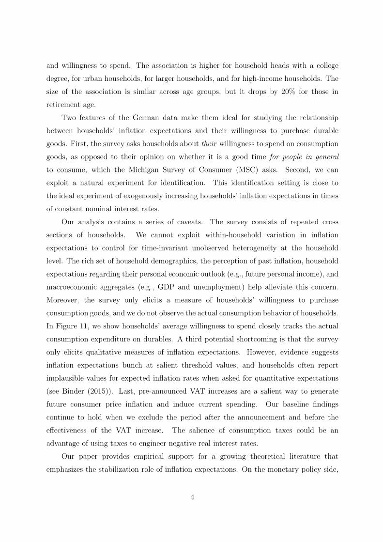
Figure 2 is a time-series plot of the fraction of households that expect higher inflation,

and of the average willingness to buy durable goods. Higher values correspond to a higher

propensity to spend. Expected inflation increases hover around the time-series mean at

the beginning of the sample, and then spike in 2001 before dropping and staying below the

mean until 2005. A sharp increase in expected inflation occurs in 2006, with a subsequent

drop and two minor spikes in mid-2007 and 2008. The series fluctuates around its mean

for the rest of the sample. The propensity to purchase durables drops below the mean in

2001. The series increases slightly before a sharp increase in 2006. The increase reverts

in 2007. The series starts trending upward at the end of 2008.

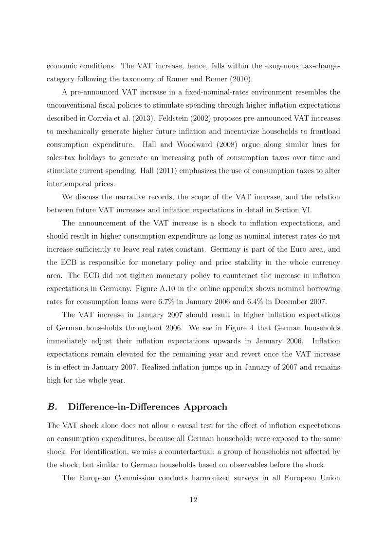
The top-left panel of Figure 3 plots the time series of the harmonized German CPI

inflation rate in percent at an annual rate. The inflation rate is 1.5% at the beginning

of the sample and increases to 2.8% in May 2001, before it drops to 0.6% in May 2003.

Inflation fluctuates between 1% and 2% until the end of 2006. At the beginning of 2007,

the annualized inflation rate is 1.7%, and increases to 3.2% in November 2007. Inflation

remains high and above its sample mean until October 2008, before we see short periods

of negative inflation in July and September 2009. After 2009, inflation slowly increases,

and is above 1% in March 2010.

The inflation expectations in the GfK survey lead actual inflation throughout the

sample. We discuss in detail in Section VI the relation between inflation expectations

and actual inflation, willingness to purchase durables, and actual purchases.

III Baseline Analysis

A. Econometric Model

Our outcome variable of interest, households’ readiness to purchase durable goods,

derives from discrete, non-ordered choices in a survey. We therefore model the response

probabilities in a multinomial-logit setting.

We assume the answer to the question on the readiness to spend is a random variable

representing the underlying population. The random variable may take three values,

y ∈ {0, 1, 2}: 0 denotes it is neither a good nor a bad time to purchase durable goods;

1 denotes it is a bad time to purchase durable goods, and 2 denotes it is a good time to

purchase durable goods.

8

We define the response probabilities as P (y = t|X), where t = 0, 1, 2, and X is a

N × K vector where N is the number of survey participants. The first element of X

is a unit vector, and the other K − 1 columns represent a rich set of household-level

observables, including demographics and expectations. The set of observables X allows

us to control for heterogeneity across households in purchasing propensities, which may

be correlated with inflation expectations.

We assume the distribution of the response probabilities is

P (y = t|X) =eXβt

1 +∑

z=1,2 eXβz

(1)

for t = 1, 2, and βt is a K × 1 vector of coefficients. The response probability for the case

y = 0 is determined, because the three probabilities must sum to unity

P (y = 0|X) =1

1 +∑

z=1,2 eXβz

. (2)

We estimate the model via maximum likelihood to obtain the vector βt of coefficients for

t = 1, 2, and set the category y = 0 as the baseline response.

We compute the marginal effects of changes in the covariates on the probability that

households choose any of three answers in the survey.

For approximately continuous covariates, we can compute the marginal effect of each

covariate x on the response probability as the derivative of P (y = t|x) with respect to x :

∂P (y = t|x)

∂x= P (y = t|x)

[βtx −

∑z=0,1,2

P (y = z|x)βzx

], (3)

for z = 0, 1, 2. For discrete covariates, we calculate marginal effects by predicting the

response probabilities for the potential values of the covariates, and compute the average

across predicted probabilities.

B. Baseline Estimation

Table 2 reports the average marginal effects computed from the multinomial logit

regressions. We cluster standard errors at the quarter level (56 clusters) to allow

for correlation of unknown form in residuals across contiguous months. In the first

9

two columns, the inflation-increase dummy is the only explanatory variable. Column

(1) reports the marginal effect of the inflation-increase dummy on the likelihood that

households respond, “it’s a bad time to buy durables,” whereas column (2) reports

the marginal effect on the likelihood that households reply, “it’s a good time to buy

durables.” Both marginal effects are positive and statistically significant. Column (2)

implies households that expect increasing inflation over the following 12 months are on

average 6.2% more likely to answer, “it’s a good time to buy durables” compared to

households that expect constant or decreasing inflation. Households with higher inflation

expectations also seem to have a higher propensity to say, “it’s a bad time to buy durables”

compared to other households. This result disappears once we control for expectations

about other outcomes, as we discuss below.

Perceptions of past inflation shape households’ expectations about future inflation

(Jonung (1981)). Controlling for past inflation perceptions reduces the marginal effect

on the negative consumption propensity, and increases the marginal effect on the

positive consumption propensity (see columns (3) and (4)). High perceptions of past

inflation decrease the marginal propensity to consume durables, whereas they increase

consumers’ negative attitude toward buying durables, consistent with the consumption

Euler equation.

Households differ in their purchasing propensity (see, e.g., Attanasio and Weber

(1993)). Household characteristics that determine purchasing propensity and inflation

expectations might be systematically related, and hence controlling for the observed

heterogeneity across households is important. We add a rich set of demographics,

expectations about personal and macroeconomic variables, and contemporaneous

macroeconomic variables. Adding demographics has little impact on the statistical

significance and economic magnitude of the effect of higher inflation expectations on

the willingness to purchase durables (columns (5) and (6)). Controlling for households’

expectations regarding their own prospects or future macroeconomic variables (columns

(7) and (8)) increases the marginal effect of the inflation-increase dummy on the “good

time” outcome. It reduces the marginal effect on the “bad time” outcome to zero.

Households that expect higher inflation are on average 8.9% more likely to have positive

spending attitudes compared to households that expect constant or decreasing inflation.

Adding contemporaneous macroeconomic variables in columns (9) and (10) does not affect

10

these findings.12

Economically, a back-of-the-envelope calculation implies that the marginal effect of

inflation expectations on the willingness to buy durables translates into 4.8% higher

real durable consumption expenditure if all Germans expect higher inflation. To reach

this suggestive conclusion, we regress the natural logarithm of real durable consumption

expenditure at the quarterly frequency on the end-of-quarter value of the average durable

purchasing propensity and quarterly dummies, and multiply the resulting coefficient of

0.5396 with the marginal effect of 8.88% (column (8) of Table 2).

Table 3 studies the role of household-level expectations in more detail. Columns

(1) to (4) split the sample based on the median perception of households regarding their

financial situation. Columns (5) to (8) split the sample based on the median expectations

of households regarding their future financial situation.13 The probability of responding

that it is a good time to purchase durables is about 6%–8% higher for households that

expect inflation to increase compared to households that expect constant or decreasing

inflation across specifications (columns (2), (4), (6), and (8)). Note the positive marginal

effect of inflation expectations on replying that it’s a bad time to buy durables is solely

driven by households with a negative perception regarding their financial situation or with

a negative outlook (compare columns (3) and (7) to columns (1) and (5)).

IV Natural Experiment and Identification Strategy

A. Exogenous Shock to Inflation Expectations

We need an exogenous shock to inflation expectations – which does not affect households’

willingness to purchase durable goods through other channels – to establish a causal link

on the readiness to buy durables. We attempt to get close to such an ideal shock following

a narrative approach (see Romer and Romer (2010)).

In November 2005, the newly-formed German government unexpectedly announced a

three-percentage-point increase in the VAT effective January 2007. The narrative records

show the VAT increase was legislated to consolidate the federal budget unrelated to future

12Table A.1 in the appendix reports marginal effects for all control variables.13The discrete nature of the survey with five possible answers results in unbalanced samples when we

use the median answer as the cutoff. Results are virtually identical when we assign households withmedian expectations to the sample with a positive economic outlook (see Table A.3).

11

economic conditions. The VAT increase, hence, falls within the exogenous tax-change-

category following the taxonomy of Romer and Romer (2010).

A pre-announced VAT increase in a fixed-nominal-rates environment resembles the

unconventional fiscal policies to stimulate spending through higher inflation expectations

described in Correia et al. (2013). Feldstein (2002) proposes pre-announced VAT increases

to mechanically generate higher future inflation and incentivize households to frontload

consumption expenditure. Hall and Woodward (2008) argue along similar lines for

sales-tax holidays to generate an increasing path of consumption taxes over time and

stimulate current spending. Hall (2011) emphasizes the use of consumption taxes to alter

intertemporal prices.

We discuss the narrative records, the scope of the VAT increase, and the relation

between future VAT increases and inflation expectations in detail in Section VI.

The announcement of the VAT increase is a shock to inflation expectations, and

should result in higher consumption expenditure as long as nominal interest rates do not

increase sufficiently to leave real rates constant. Germany is part of the Euro area, and

the ECB is responsible for monetary policy and price stability in the whole currency

area. The ECB did not tighten monetary policy to counteract the increase in inflation

expectations in Germany. Figure A.10 in the online appendix shows nominal borrowing

rates for consumption loans were 6.7% in January 2006 and 6.4% in December 2007.

The VAT increase in January 2007 should result in higher inflation expectations

of German households throughout 2006. We see in Figure 4 that German households

immediately adjust their inflation expectations upwards in January 2006. Inflation

expectations remain elevated for the remaining year and revert once the VAT increase

is in effect in January 2007. Realized inflation jumps up in January of 2007 and remains

high for the whole year.

B. Difference-in-Differences Approach

The VAT shock alone does not allow a causal test for the effect of inflation expectations

on consumption expenditures, because all German households were exposed to the same

shock. For identification, we miss a counterfactual: a group of households not affected by

the shock, but similar to German households based on observables before the shock.

The European Commission conducts harmonized surveys in all European Union

12

countries. We obtained access to the confidential micro data for three additional countries

(France, Sweden, and the United Kingdom) through national statistical offices and GfK

subsidiaries.14 We use the households in these three countries to construct our control

group.

Our identification strategy is a difference-in-differences approach: we compare

German households’ readiness to purchase durables with that of households in other

European countries, before and after the VAT shock.

We estimate the average treatment effect (ATE) of the VAT shock on the readiness

to purchase durables as

(DurGerman, post −DurGerman, pre)− (Durforeign, post −Durforeign, pre), (4)

where DurGerman, post is German households’ average readiness to purchase durable goods

after the announcement of the VAT increase, DurGerman, pre is German households’

average readiness to purchase durables goods before the announcement of the VAT

increase, and Durforeign, post and Durforeign, pre are the analogous averages for foreign

households not exposed to the VAT shock.

C. Identifying Assumptions

The parallel-trends assumption is a necessary condition for identification. It requires

that our control group behaves similarly to German households before the announcement

of the VAT increase. Under this assumption, we can interpret the evolution of

inflation expectations and consumption behavior of matched foreign households after

the announcement as a valid counterfactual to the evolution of the behavior of German

households absent the VAT shock.

The top panels of Figure 5 and Figure 6 provide graphical evidence that the parallel-

trend assumption seems satisfied in our setting. The trends in inflation expectations

and purchasing propensities are parallel for German and foreign households before the

announcement of the VAT increase (November 2005). Starting in January 2006, both the

inflation expectations and willingness to buy durable goods of German households start

to increase substantially. Trends for foreign households do not move compared to the

14The online appendix contains details of the data sources and the surveys used in national language.

13

pre-shock period. We see in the bottom panels of Figure 5 and Figure 6 that the similarity

of pre-shock trends is even more pronounced when we only use French households as a

control group. France and Germany face the same monetary policy, they share a common

border, and are structurally similar.

We verify in Table 4 that households in each of the three foreign countries

unconditionally display a positive association between inflation expectations and

consumption expenditure similar to German households. Foreign households are therefore

likely to react to increases in inflation expectations in a similar fashion as German

households.

We match each German household in each month with a household in another

country, interviewed in the same month, with similar demographic characteristics. We

use a nearest-neighbor algorithm to match households based on propensity scores.15 We

estimate propensity scores with a logit regression of the treatment indicator on gender,

age, education, income, and social status.16 Our samples are repeated cross sections, and

we cannot track German and matched foreign households before and after the shock. We

perform a second level of matching, which pairs up similar households interviewed before

and after the shock separately within the German and the foreign survey waves.

The matching exercise is meaningful only for German and foreign households in the

common support of the distributions of the propensity score for the two groups. In Figure

7, we plot the distribution of the propensity score for the treatment group (red) and the

control group (blue). Households are distributed across the full range of the propensity

score in both groups.

Moreover, we formally test whether households’ characteristics are balanced after

the matching process. In Table 5, we report the mean of the matching categories

for households in the control group and treated group as of June 2005, our baseline

month before the announcement of the VAT increase. Columns (3) and (4) test the null

hypothesis that the means across the two groups are equal. We cannot reject the null for

any of the five matching variables.

15All the results are virtually identical if we perform the monthly matching using a group of controlhouseholds for each German household, and we minimize the difference in observables of the Germanhousehold and the group of foreign households.

16We show in subsection V below that age, income, and education are the strongest determinantsof cross-sectional heterogeneity in the relation between households’ inflation expectations and theirconsumption behavior.

14

All our results are similar or become stronger if we only use households from France

as a control group. Neither inflation expectations nor nominal rates changed in the UK

and Sweden during 2006, and using a larger pool of control households increases the size of

the common support, and improves the balancing of matched households’ characteristics

ex post.

D. Threats to Identification

Changes in VAT might affect households’ decisions to purchase durables through channels

different from inflation expectations. A positive average treatment effect in equation (4)

might reflect those other channels, in which case we could interpret our finding only as

an impulse response of consumption expenditure to the announcement of a VAT increase,

as opposed to the causal effect of inflation expectations on consumption expenditure. We

test below whether the VAT shock affected households’ expectations other than inflation

expectations, which might affect the readiness to spend on durables irrespective of inflation

expectations.

Table 3 documents that the perception of past income and the expectation of

future individual income are important determinants of the marginal effects of inflation

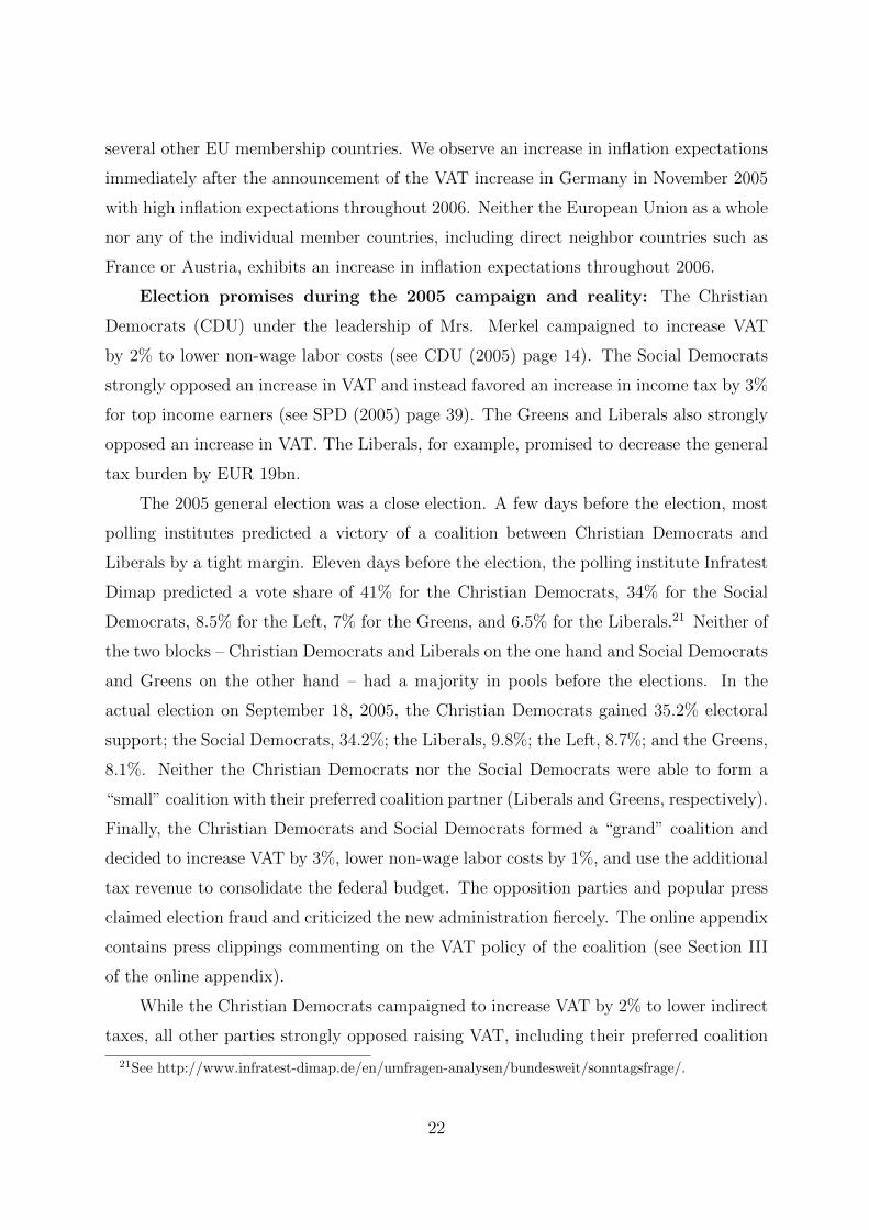
expectations on consumption choices. Figure 8 plots the evolution of average income

perceptions and income expectations together with inflation expectations to test whether

improved income perceptions or improved income expectations after the announcement

to increase VAT might drive our findings. The announcement of the VAT increase does

immediately increase average inflation expectations, whereas the average perception of

income and the average expectation of future income do not move.

We cannot test whether the announcement of an increase in VAT affected all channels

different from inflation expectations, because most of these channels are unobservable.

Figure 8, however, shows household expectations regarding future income and the

perception of current income, which are important determinants of individual purchasing

behavior, are unlikely to drive a potentially positive average treatment effect in equation

(4).

15

E. Causal Effect of VAT Shock on Readiness to Spend

We run a set of cross-sectional regressions on the matched sample before and after the

announcement of the VAT increase to estimate the average treatment effect of the VAT

shock in equation (4). We set the reference month to June 2005, and we change the end

month m across regressions.17

We estimate the following specification:

∆Duri, 06/2005→m = α + βm × V ATshocki + ∆X ′i, 06/2005→m × γ + εi, (5)

where ∆Duri, 06/2005→m is the difference in the willingness to spend on durable goods

between month m and June 2005, V ATshocki is an indicator equal to 1 if the household

was exposed to the VAT shock, βm captures the effect of the VAT shock on the willingness

to buy durables for household i in month m, and ∆X ′i,06/2005→m is the difference in a set

of observables between month m and the baseline month. To economize on notation, we

use the same indicator i for matched households interviewed in different months.

Figure 9 plots the estimated coefficient βm (solid line) of equation (5) for each month

m from July 2005 to December 2007, and the 95% confidence intervals (dashed line).

We find no difference in the readiness to spend on durable goods between German and

matched households before the announcement of the VAT increase. Starting in December

2005, the VAT shock results in a positive effect on the willingness of German households to

purchase compared to matched households: German households are 3.8 percentage points

(s.e. 1.5 percentage points) more likely to declare that it is a good time to purchase

durable goods after the announcement compared to before, and compared to matched

foreign households. The effect increases in magnitude throughout 2006 and peaks at

34 percentage points in November 2006. The average treatment effect drops to zero in

January 2007 once VAT increases and higher inflation materializes.18

Figure 9 shows that the VAT shock has a strong and positive effect on the willingness

of German households to purchase durable goods after the announcement and before

the increase took effect, even after controlling for the purchasing propensities of similar

17All the results are similar if we use any other month before the announcement of the VAT increasein November 2005.

18Figure A.3 in the online appendix plots the average treatment effect of a specification in which wealso match on income expectations for the next 12 months in addition to gender, age, education, income,and social status. Results are virtually identical.

16

households not exposed to the shock in a difference-in-differences setting. Interestingly,

we do not detect any reversal of the positive effect of the VAT shock on the willingness

to purchase durable goods after January 2007.

V Heterogeneity of the Effects

A. Household Heterogeneity

In this section, we study the role of demographics in shaping the marginal effect of inflation

expectations on consumption expenditure.

We first look at education. Germany has a three-tier school system, and pupils

choose their secondary education track after four years of primary school. Hauptschule

offers a total of 9 years of basic education, Realschule offers 10 years, and Gymnasium

offers 13 years, concluding with A levels (required to enter college). Table 6 studies

the relationship between inflation expectations and the willingness to spend on durables

separately for household heads with different levels of education. Survey participants

with a Hauptschule degree who expect inflation to increase are 6.9% more likely to have

a positive stance toward buying durables compared to households that expect constant

or decreasing inflation (column (2)). This marginal effect increases with education, and

is more than 60% larger for household heads that hold a college degree (columns (4), (6),

(8)).

Lifetime inflation experiences matter for how recent inflation shapes inflation

expectations of young and old households (see Malmendier and Nagel (2009)). Retirees

have different time-use and consumption patterns compared to the working-age population

(see Aguiar and Hurst (2005)) and typically have nominal pensions in Germany, hold few

real assets, and have lower human capital compared to someone in the labor force. The

marginal effect of inflation increases on the willingness to spend is constant across age

groups, but drops for those aged 65 or higher. Household heads between 14 to 65 that

expect inflation to increase are 9% more likely to buy durables compared to households

that expect constant or decreasing inflation (Table 7, columns (2), (4), (6), (8)). This

effect is about 20% lower for households in retirement age (column (10)).

City size, marital status, and household size might shape the effect of inflation

expectations on consumption expenditure through financial literacy (see, e.g., Lusardi

17

and Mitchell (2011) and Campbell (2006)). Table 8 shows the marginal effect is about

40% lower for households living in rural areas than households in large cities (columns (2),

(4), (6)). In Table 9, richer survey participants with a monthly net income above EUR

2,500 possess a 15% to 20% higher marginal effect of inflation increases on the likelihood

to reply, “it’s a good time to buy durables” (column (6)), compared to survey participants

with less than EUR 2,500 monthly net income (columns (2) and (4)).

Table 10 looks at financial constraints. Hand-to-mouth consumers might think it is a

good time to purchase durables in times of high inflation, but might be unable to substitute

intertemporally (see Campbell and Mankiw (1989)). Following Zeldes (1989) and Kaplan,

Violante, and Weidner (2014), we split the sample to households that currently save and

households that dis-save or take on debt. Table 10 shows the marginal effect of higher

inflation expectations on the willingness to purchase durable goods is about 40% larger

for unconstrained households compared to hand-to-mouth consumers.

B. Effect over Time

Households may perceive it is a favorable time to purchase durable goods for several

reasons, including low prices, expected price increases, low nominal interest rates,

generally good economic times, or prosperous times for the household. The motive to

purchase durable goods because of higher future prices and lower real interest rates is likely

to be more important and salient just before an announced increase in VAT compared to

other reasons. We therefore expect to find a larger marginal effect of inflation expectations

on purchasing propensities in 2006.

Figure 1 shows the marginal effect of inflation expectations on purchasing propensities

is especially high in 2006. Table 11 studies this relationship using micro data to control

for household characteristics and expectations. From November 2005 to December 2006,

households that expect inflation to increase are 19% more likely to have a positive spending

attitude. Our baseline findings continue to hold when we exclude the period November

2005 to December 2006 (see columns (3) and (4)). We do not find different marginal

effects when we study the time period of the European financial debt crisis in columns (5)

and (6). We estimate our baseline specification year-by-year and plot the marginal effect

in Figure 10. The marginal effect is around 5%–6% throughout the sample but spikes in

2006.

18

C. Additional Results

The online appendix reports additional results and robustness checks. Households that

expect inflation to increase are also more likely to answer that it is a bad time to

save, consistent with the consumption Euler equation (see Table A.7). Results are

quantitatively and statistically similar when we split the sample based on expectations

regarding macroeconomic aggregates such as GDP or unemployment, when we use

dummy-variable specifications for past inflation perceptions and expected inflation, when

we estimate a linear probability or an ordered probit model, when we add month and year

fixed effects, and when we exclude past inflation perception from the set of covariates. We

also show that households that expect deflation are on average more likely to say that it

is a bad time to buy compared to households that expect constant or increasing inflation.

GfK also asks households on a quarterly basis whether they want to spend more, the same

amount, or less for specific consumption goods in the following 12 months compared to

the previous 12 months. We find that households which expect inflation to increase want

to spend more on cars, furniture, appliances, and renovations to their house. The effect

does not seem to differ across genders and across households with or without children.

We find similar marginal effects for single, couple, married, and divorced households.

Renters have a slightly higher marginal effect than house- or apartment-owners. Full-time

employed survey participants have a higher marginal effect than part-time employed and

unemployed survey participants.

VI Discussion

In section III, we document that households with higher inflation expectations are more

willing to purchase durable goods. The answer to the question we posed at the beginning of

the paper might, therefore, be an affirmative yes: temporarily higher inflation expectations

could indeed stimulate current consumption spending. However, a few important points

should be discussed before we can infer any policy recommendations from our analysis.

Willingness to spend versus actual spending: We are ultimately interested in

how inflation expectations transmit to actual consumption. Our survey only reports

the willingness to purchase durable goods. Figure 11 shows the time series of the

average readiness to purchase durable goods across households and realized real durable

19

consumption growth at the quarterly frequency in Germany track each other closely.19

Figure 12 is a scatter plot of the cyclical components of log real durable consumption and

the average propensity to purchase durables.20 Real and reported spending on durables

are positively related with a correlation of 0.46.

The reported willingness to purchase has potential advantages compared to measures

of actual expenditures elicited with surveys. Spending data in surveys typically contain

noise, because survey participants might not recall their actual purchases, or they might

overstate their purchases of visible products such as cars and understate the consumption

of “sin” products, such as tobacco and alcohol (see Hurd and Rohwedder (2012) and

Atkinson and Micklewright (1983)).

Durable consumption versus GDP: Academics and policy makers typically

advocate temporarily higher inflation expectations during a liquidity trap to stimulate

GDP. The ultimate aim is to bring the economy back to its long-run steady-state

growth path. We document that households with higher inflation expectations are

more willing to purchase durable goods, but we do not observe whether households

cut back on other components of consumption. Households that expect higher inflation

are less likely to save, which suggests that they increase total consumption (see Table

A.7 in the online appendix). We also do not study how inflation expectations affect

firm investment. Evidence for aggregate real GDP growth (Figure A.1) suggests higher

inflation expectations might have indeed increased aggregate demand, because real GDP

growth increased from 1.6% in the last quarter of 2005 to 4.38% in the last quarter of

2006.

Temporary versus permanent increases in inflation expectations: We focus

our discussion on temporary increases of inflation expectations to stimulate consumption.

Some economists have suggested unexpectedly increasing inflation to “inflate away”

government debt and delever household balance sheets. Blanchard, Dell’Ariccia, and

Mauro (2010) and Ball (2013), on the contrary, recommend permanently higher inflation

targets to lower the probability of hitting the zero-lower bound on nominal interest rates.

Our evidence does not speak to the positive or negative effects of permanently higher

19We use the end-of-quarter value of the index to construct a quarterly series. We get similar resultsif we plot the average within a quarter or use the first or second monthly observation within a quarter.

20We use a Hodrick-Prescott filter with smoothing parameter λ of 1,600 to extract the cyclicalcomponent.

20

inflation targets, whether expected or unexpected, on welfare. Hilscher, Raviv, and Reis

(2014) suggest unexpected higher inflation is unlikely to lower real debt significantly.

Mishkin (2011) argues the occurrence of zero-lower-bound periods is too rare to justify

the cost of higher inflation. Findings by Gorodnichenko and Weber (2015), Weber (2015),

and D’Acunto, Liu, Pflueger, and Weber (2015) suggest substantial costs of nominal

price adjustment. Ultimately, Coibion, Gorodnichenko, and Wieland (2012) and Ascari,

Phaneuf, and Sims (2015) derive the optimal inflation rate in a New Keynesian model

with infrequent occurrences at the zero lower bound, and conclude the welfare-optimal

inflation rate is below 2%.

Fiscal versus monetary policy: Macro models often rely on monetary policy to

engineer higher inflation expectations. Our survey data do not allow us to identify the

origin of the cross-sectional heterogeneity in inflation expectations. When we use the

unexpected increase in VAT as a shock to inflation expectations, we can trace the cause

of higher inflation expectations back to fiscal policy. Our findings might therefore not

speak to the effects of higher inflation expectations induced by monetary policy. Our

baseline findings hold when we exclude the period after the announcement and before the

effectiveness of the VAT increase, which alleviates those considerations.

Reduced and full VAT tax: All services and products in Germany are subject to

a value-added tax that is part of the European VAT system. The general tax rate was

16% until December 2006 and increased to 19% in 2007. A reduced rate of 7% applies

to many convenience goods such as food, books, or flowers. The reduced rate has been

unchanged since 1983. Rent, services for non-profit organizations, and medical expenses

are not subject to VAT.

VAT increase as a shock to inflation: Prices in Germany are typically

tax-inclusive; that is posted prices are gross prices including value-added tax. Many

convenience goods are only subject to a reduced VAT. If the VAT increase of 2007

indeed led to an increase in inflation, we should observe an immediate rise in inflation

for durable goods that are subject to full VAT, whereas we should see a smaller response

for non-durable inflation. The lower left panel of Figure 3 shows an immediate increase

in durable-goods inflation, which remained high and increased throughout 2007. On the

contrary, the lower-right panel shows a constant non-durable-goods inflation rate during

2007. Figure A.2 plots inflation expectations for the European Union (EU), Germany, and

21

several other EU membership countries. We observe an increase in inflation expectations

immediately after the announcement of the VAT increase in Germany in November 2005

with high inflation expectations throughout 2006. Neither the European Union as a whole

nor any of the individual member countries, including direct neighbor countries such as

France or Austria, exhibits an increase in inflation expectations throughout 2006.

Election promises during the 2005 campaign and reality: The Christian

Democrats (CDU) under the leadership of Mrs. Merkel campaigned to increase VAT

by 2% to lower non-wage labor costs (see CDU (2005) page 14). The Social Democrats

strongly opposed an increase in VAT and instead favored an increase in income tax by 3%

for top income earners (see SPD (2005) page 39). The Greens and Liberals also strongly

opposed an increase in VAT. The Liberals, for example, promised to decrease the general

tax burden by EUR 19bn.

The 2005 general election was a close election. A few days before the election, most

polling institutes predicted a victory of a coalition between Christian Democrats and

Liberals by a tight margin. Eleven days before the election, the polling institute Infratest

Dimap predicted a vote share of 41% for the Christian Democrats, 34% for the Social

Democrats, 8.5% for the Left, 7% for the Greens, and 6.5% for the Liberals.21 Neither of

the two blocks – Christian Democrats and Liberals on the one hand and Social Democrats

and Greens on the other hand – had a majority in pools before the elections. In the

actual election on September 18, 2005, the Christian Democrats gained 35.2% electoral

support; the Social Democrats, 34.2%; the Liberals, 9.8%; the Left, 8.7%; and the Greens,

8.1%. Neither the Christian Democrats nor the Social Democrats were able to form a

“small” coalition with their preferred coalition partner (Liberals and Greens, respectively).

Finally, the Christian Democrats and Social Democrats formed a “grand” coalition and

decided to increase VAT by 3%, lower non-wage labor costs by 1%, and use the additional

tax revenue to consolidate the federal budget. The opposition parties and popular press

claimed election fraud and criticized the new administration fiercely. The online appendix

contains press clippings commenting on the VAT policy of the coalition (see Section III

of the online appendix).

While the Christian Democrats campaigned to increase VAT by 2% to lower indirect

taxes, all other parties strongly opposed raising VAT, including their preferred coalition

21See http://www.infratest-dimap.de/en/umfragen-analysen/bundesweit/sonntagsfrage/.

22

partner, the Liberals. At the same time, the outcome of the election was unclear until

the actual election. A VAT increase by 3% for fiscal consolidation was therefore certainly

unexpected. Figure 2 is direct evidence that households did not expect higher inflation:

households’ inflation expectation did not increase until December 2005 after the new

administration announced its plans to increase VAT.

VII Concluding Remarks

We document a positive cross-sectional association between households’ inflation

expectations and their willingness to purchase durable consumption goods using novel

German survey data. Households that expect higher inflation are 8% more likely to have

a positive attitude toward buying durable consumption goods compared to households

that expect constant or decreasing inflation. The German setting allows the use of the

unexpected announcement of a VAT increase in 2005 as an exogenous shock to inflation

expectations, which we exploit for identification. We use households in other European

countries to form a control group not exposed to the shock. This difference-in-differences

analysis confirms our baseline finding.

The effect of inflation expectations on consumption behavior is stronger for more

educated, working-age, high-income, and urban households and builds up in 2006 after

the announcement and before the effectiveness of the VAT increase. Our results provide

the first empirical evidence using survey data at the household level that temporarily

higher inflation expectations might stimulate consumption expenditure in a fixed nominal

interest rate environment, such as during a liquidity trap or in a currency union.

The heterogeneous marginal effect of inflation expectations on consumption behavior

across households, and the temporal buildup of the effect in 2006, may represent

major impediments to the transmission of economic and monetary policies that

target households’ consumption and savings behaviors and might result in unintended

consequences such as a redistribution of wealth. Future studies should examine

which household characteristics, such as limited attention or cognitive abilities, hinder

households from updating expectations about future macroeconomic variables to policy

interventions.

23

References

Aguiar, M. and E. Hurst (2005). Consumption versus expenditure. Journal of PoliticalEconomy 113 (5), 919–948.

Aruoba, S. B. and F. Schorfheide (2011). Sticky prices versus monetary frictions: Anestimation of policy trade-offs. American Economic Journal: Macroeconomics 3 (1),60–90.

Ascari, G., L. Phaneuf, and E. Sims (2015). On the welfare and cyclical implications ofmoderate trend inflation. Technical report, National Bureau of Economic Research.

Atkinson, A. B. and J. Micklewright (1983). On the reliability of income data in thefamily expenditure survey 1970-1977. Journal of the Royal Statistical Society. Series A(General) 146 (1), 33–61.

Attanasio, O. P. and G. Weber (1993). Consumption growth, the interest rate andaggregation. The Review of Economic Studies 60 (3), 631–649.

Bachmann, R., T. O. Berg, and E. Sims (2015). Inflation expectations and readiness tospend: cross-sectional evidence. American Economic Journal: Economic Policy 7 (1),1–35.

Baker, S. R., N. Bloom, and S. J. Davis (2014). Measuring economic policy uncertainty.Unpublished Manuscript, Stanford University .

Ball, L. (2013). The case for four percent inflation. Central Bank Review 13 (2), 17–31.Binder, C. (2015). Consumer inflation uncertainty and the macroeconomy: evidence from

a new micro-level measure. Unpublished Manuscript, UC Berkeley .Blanchard, O., G. Dell’Ariccia, and P. Mauro (2010). Rethinking macroeconomic policy.

Journal of Money, Credit and Banking 42 (6), 199–215.Bloom, N. (2009). The impact of uncertainty shocks. Econometrica 77 (3), 623–685.Burke, M. A. and A. Ozdagli (2014). Household inflation expectations and consumer

spending: evidence from panel data. Unpublished Manuscript, Federal Reserve Bank ofBoston 13 (25), 1–43.

Campbell, J. Y. (2006). Household finance. The Journal of Finance 61 (4), 1553–1604.Campbell, J. Y. and N. G. Mankiw (1989). Consumption, income and interest rates:

Reinterpreting the time series evidence. In NBER Macroeconomics Annual 1989,Volume 4, pp. 185–216. MIT Press.

Carvalho, C. and F. Nechio (2014). Do people understand monetary policy? Journal ofMonetary Economics 66, 108–123.

Cashin, D. and T. Unayama (2015). Measuring intertemporal substitution inconsumption: evidence from a VAT increase in Japan. Review of Economics andStatistics (forthcoming).

CDU (2005). Deutschlands Chancen nutzen. Wachstum. Arbeit. Sicherheit. ElectoralManifest .

Christiano, L., M. Eichenbaum, and S. Rebelo (2011). When is the government spendingmultiplier large? Journal of Political Economy 119 (1), 78–121.

Coibion, O. and Y. Gorodnichenko (2012). What can survey forecasts tell us aboutinformation rigidities? Journal of Political Economy 120 (1), 116–159.

Coibion, O. and Y. Gorodnichenko (2015). Is the Phillips curve alive and well afterall? Inflation expectations and the missing disinflation. American Economic Journal:Macroeconomics 7 (1), 197–232.

Coibion, O., Y. Gorodnichenko, and J. Wieland (2012). The optimal inflation rate in newkeynesian models: Should central banks raise their inflation targets in light of the zerolower bound? Review of Economic Studies 79 (4), 1371–1406.

Correia, I., E. Farhi, J. P. Nicolini, and P. Teles (2013). Unconventional fiscal policy at

24

the zero bound. American Economic Review 103 (4), 1172–1211.D’Acunto, F., R. Liu, C. Pflueger, and M. Weber (2015). Flexible prices and leverage.

Unpublished manuscript, University of Chicago Booth School of Business .Doepke, M. and M. Schneider (2006). Inflation and the redistribution of nominal wealth.

Journal of Political Economy 114 (6), 1069–1097.Drager, L. and M. J. Lamla (2013). Anchoring of consumers’ inflation expectations:

Evidence from microdata. Unpublished Manuscript, University of Hamburg .Eggertsson, G. B. (2006). The deflation bias and committing to being irresponsible.

Journal of Money, Credit and Banking 38 (2), 283–321.Eggertsson, G. B. (2008). Great expectations and the end of the depression. The American

Economic Review 98 (4), 1476–1516.Eggertsson, G. B. (2011). What fiscal policy is effective at zero interest rates? In NBER

Macroeconomics Annual 2010, Volume 25, pp. 59–112. University of Chicago Press.Eggertsson, G. B. and M. Woodford (2003). The zero bound on interest rates and optimal

monetary policy. Brookings Papers on Economic Activity 34 (1), 139–235.Farhi, E. and I. Werning (2015). Fiscal multipliers: Liquidity traps and currency unions.

Unpublished Manuscript, MIT .Feldstein, M. (2002). The role for discretionary fiscal policy in a low interest rate

environment. Technical report, National Bureau of Economic Research.Gorodnichenko, Y. and M. Weber (2015). Are sticky prices costly? Evidence from the

stock market. American Economic Review (forthcoming).Hall, R. and S. Woodward (2008, December 11). Measuring the effect of infrastructure

spending on GDP, Financial Crisis and Recession (blog).Hall, R. E. (2011). The long slump. American Economic Review 101 (2), 431–69.Hausman, J. K. and J. F. Wieland (2014). Abenomics: preliminary analysis and outlook.

Brookings Papers on Economic Activity 2014 (1), 1–63.Hilscher, J., A. Raviv, and R. Reis (2014). Inflating away the public debt? An empirical

assessment. Technical report, National Bureau of Economic Research.Hurd, M. D. and S. Rohwedder (2012). Measuring total household spending in a monthly

internet survey: Evidence from the American Life Panel. Technical report, NationalBureau of Economic Research.

Ichiue, H. and S. Nishiguchi (2015). Inflation expectations and consumer spending at thezero bound: micro evidence. Economic Inquiry 53 (2), 1086–1107.

Jalil, A. and G. Rua (2015). Inflation expectations and recovery from the depression in1933: Evidence from the narrative record. Unpublished Manuscript, Federal ReserveBoard .

Jonung, L. (1981). Perceived and expected rates of inflation in Sweden. The AmericanEconomic Review 71 (5), 961–968.

Kaplan, G., G. L. Violante, and J. Weidner (2014). The wealthy hand-to-mouth. Technicalreport, National Bureau of Economic Research.

Krugman, P. R. (1998). It’s baaack: Japan’s slump and the return of the liquidity trap.Brookings Papers on Economic Activity 1998 (2), 137–205.

Lusardi, A. and O. S. Mitchell (2011). Financial literacy and retirement planning in theUnited States. Journal of Pension Economics and Finance 10 (4), 509–525.

Malmendier, U. and S. Nagel (2009). Learning from inflation experiences. Unpublishedmanuscript, UC Berkeley .

Mian, A., K. Rao, and A. Sufi (2013). Household balance sheets, consumption, and theeconomic slump. The Quarterly Journal of Economics 128 (4), 1687–1726.

Mishkin, F. S. (2011). Monetary policy strategy: lessons from the crisis. Technical report,

25

National Bureau of Economic Research.Pastor, L. and P. Veronesi (2013). Political uncertainty and risk premia. Journal of

Financial Economics 110 (3), 520–545.Piazzesi, M. and M. Schneider (2009). Momentum traders in the housing market: survey

evidence and a search model. The American Economic Review 99 (2), 406–411.Romer, C. D. and D. H. Romer (2010). The macroeconomic effects of tax changes:

estimates based on a new measure of fiscal shocks. The American EconomicReview 100 (3), 763–801.

Romer, C. D. and D. H. Romer (2013). The missing transmission mechanismin the monetary explanation of the Great Depression. The American EconomicReview 103 (3), 66–72.

SPD (2005). Vertrauen in Deutschland. Das Wahlmanifest der SPD. Electoral Manifest .Taylor, J. B. (2013, January 28). Fed policy is a drag on the economy. Wall Street

Journal .Weber, M. (2015). Nominal rigidities and asset pricing. Unpublished manuscript,

University of Chicago Booth School of Business .Werning, I. (2012). Managing a liquidity trap: monetary and fiscal policy. Unpublished

Manuscript, MIT .Woodford, M. (2011). Simple analytics of the government expenditure multiplier.

American Economic Journal: Macroeconomics 3 (1), 1–35.Zeldes, S. P. (1989). Consumption and liquidity constraints: an empirical investigation.

The Journal of Political Economy 97 (2), 305–346.

26

Figure 2: Expected Increase in Inflation and Average Readiness to Spend onDurables

0

0.1

0.2

0.3

0.4

0.5

Fractio

nInflatio

nIncreases

1.8

2.0

2.2

2.4

12/0

012

/01

12/0

212

/03

12/0

412

/05

12/0

612

/07

12/0

812

/09

12/1

012

/11

12/1

212

/13

Good

Tim

eto

Buy

Durables

Inflation ExpectationsDurable Purchases

This figure plots average monthly inflation expectation (blue line, left y axis) and the average monthly

readiness to purchase durables (green dashed line, right y axis) over time. We use the confidential micro data

underlying the GfK Consumer Climate MAXX survey to construct these variables. GfK asks a representative

sample of 2,000 households how consumer prices will evolve in the next twelve months compared to the

previous twelve months and whether it is a good time to purchase durables given the current economic

conditions. We create a dummy variable which equals 1 when a household expects inflation to increase. Higher

values correspond to better times to purchase durables. The sample period is January 2000 to December 2013

for a total of fourteen years.

27

Figure 3: Time Series of CPI Inflation Rate

−2%

0%

2%

4%

6%

InflationRate

[%]

12/0

012

/0112

/0212

/0312

/0412

/0512

/0612

/07

12/0

812

/0912

/1012

/1112

/1212

/13

CPI π

−2%

0%

2%

4%

6%

InflationRate

[%]

12/0

012

/0112

/0212

/0312

/0412

/0512

/0612

/0712

/08

12/0

912

/1012

/1112

/1212

/13

excl food π

−2%

0%

2%

4%

6%

InflationRate

[%]

12/0

012

/0112

/0212

/0312

/0412

/0512

/0612

/07

12/0

812

/0912

/1012

/1112

/1212

/13

Durable π

−2%

0%

2%

4%

6%

InflationRate

[%]

12/0

012

/0112

/0212

/0312

/0412

/0512

/0612

/0712

/08

12/0

912

/1012

/1112

/1212

/13

Non−durable π

This figure plots the monthly time series of the German consumer price (CPI) inflation rate π in percent

at an annual rate. The top left panel plots the harmonized overall consumer price inflation rate. The top

right panel plots all items CPI excluding food and energy. The bottom left panel plots major durables CPI.

The bottom right panel plots the non-durable households goods CPI. The sample period is January 2000 to

December 2013 for a total of fourteen years.

28

Figure 4: Standardized Lagged Inflation Expectations and CPI Inflation Rate

−2

−1

0

1

2

3

4

5

StandardizedInflation

12/0

112

/02

12/0

312

/04

12/0

512

/06

12/0

712

/08

12/0

912

/10

12/1

112

/12

12/1

3

Standardized Lagged Inflation ExpectationsStandardized Durable Inflation

This figure plots the monthly time series of the one-year lagged standardized average monthly inflation

expectation and the harmonized major durables consumer price inflation rate in percent at an annual rate. We

use the confidential micro data underlying the GfK Consumer Climate MAXX survey to construct inflation

expectations. GfK asks a representative sample of 2,000 households how consumer prices will evolve in the

next twelve months compared to the previous twelve months. We create a dummy variable which equals 1

when a household expects inflation to increase. The sample period is January 2000 to December 2013 for a

total of fourteen years.

29

Figure 5: Expected Increase in Inflation: Germany and European Union

03/0

406

/04

09/0

412

/04

03/0

506

/05

09/0

512

/05

03/0

606

/06

09/0

6

Fra

ctio

nIn.ati

on

Incr

ease

s

0

0.1

0.2

0.3

0.4

0.5

0.6

GermanyEuropean Countries

03/0

406

/04

09/0

412

/04

03/0

506

/05

09/0

512

/05

03/0

606

/06

09/0

6

Fra

ctio

nIn.ati

on

Incr

ease

s

0

0.1

0.2

0.3

0.4

0.5

0.6

GermanyFrance

This figure plots average monthly inflation expectation over time. We use the confidential micro data

underlying the GfK Consumer Climate MAXX survey to construct the variables for Germany and similar data

from national statistical agencies and GfK subsidiaries for the United Kingdom, Sweden, and France. GfK

asks a representative sample of 2,000 households how consumer prices will evolve in the next twelve months

compared to the previous twelve months. We create a dummy variable which equals 1 when a household

expects inflation to increase. The sample period is January 2004 to December 2006 for a total of three years.

30

Figure 6: Readiness to Spend on Durables: Germany and European Union

03/0

406

/04

09/0

412

/04

03/0

506

/05

09/0

512

/05

03/0

606

/06

09/0

6

Good

Tim

eto

Buy

Dura

ble

s

1

1.5

2

2.5

3

GermanyEuropean Countries

03/0

406

/04

09/0

412

/04

03/0

506

/05

09/0

512

/05

03/0

606

/06

09/0

6

Good

Tim

eto

Buy

Dura

ble

s

1

1.5

2

2.5

3

GermanyFrance

This figure plots the average monthly readiness to purchase durables over time. We use the confidential micro

data underlying the GfK Consumer Climate MAXX survey to construct these variables for Germany and

similar data from national statistical agencies and GfK subsidiaries for the United Kingdom, Sweden, and

France. GfK asks a representative sample of 2,000 households whether it is a good time to purchase durables

given the current economic conditions. Higher values correspond to better times to purchase durables. The

sample period is January 2004 to December 2006 for a total of three years.

31

Figure 7: Common Support of Treated and Matched Households

0 .2 .4 .6 .8Propensity Score

Untreated Treated

This figure plots the number of households in the untreated (blue) and treated (red) group across 40

equal-length partitions of the distribution of the propensity score in the baseline month (June 2005) for the

difference-in-differences analysis. We estimate the propensity score with a logit specification whose outcome

variable is the indicator for whether a household is in the treated or control group, and the controls are the

observables we use for the matching of households: age group, gender, education group, income group, and

social status group. The treated group includes 1,431 German households, whereas the control group includes

5,108 households from the UK, France, and Sweden.

Figure 8: Household Expectations

0

0.1

0.2

0.3

0.4

0.5

0.6

Household

Expectations

03/0

406

/04

09/0

412

/04

03/0

506

/05

09/0

512

/05

03/0

606

/06

09/0

6

Inflation ExpectationsIncome PerceptionIncome Expectations

This figure plots average monthly inflation expectation, perception of past income and expectation of future

income over time. We use the confidential micro data underlying the GfK Consumer Climate MAXX survey

to construct those variables. GfK asks a representative sample of 2,000 households how consumer prices

will evolve in the next twelve months compared to the previous twelve months, how the financial situation of

the household evolved during the past twelve months, and how the financial situation of the household will

evolve during the next twelve months. We create dummy variables which equal 1 when a household expects

inflation to increase, perceives an improved financial situation, and expects an improved financial situation.

The sample period is January 2004 to December 2006 for a total of three years.

32

Figure 9: Readiness to Spend: German vs. Foreign Households

09/0

512

/05

03/0

606

/06

09/0

612

/06

03/0

706

/07

09/0

7

Avera

ge

Tre

atm

ent

E,ect

-0.1

-0.05

0

0.05

0.1

0.15

0.2

0.25

0.3

0.35

0.4

Average Treatment Effect Over TimeTwo-Standard Error Bounds

This figure plots βm coefficient (solid line) of ∆Duri,06/2005→m = α+βm×V ATshocki+∆X ′i,06/2005→m×γ+εiand two standard deviation error bands (dashed line). ∆Duri,06/2005→m is the difference in the willingness to

spend on durable goods between month m and June 2005, V ATshocki is an indicator which equals 1 if the

household was exposed to the VAT shock, βm captures the effect of the VAT shock on the willingness to buy

durables for household i in month m, and ∆X ′i,06/2005→m is the difference in a set of observables between

month m and the baseline month. We use the micro data underlying the Directorate-General for Economic and

Financial Affairs of the European Commission harmonized consumer surveys to construct these variables.

Figure 10: Readiness to Spend and Inflation Expectations Over Time

0

0.02

0.04

0.06

0.08

0.1

0.12

0.14

0.16

0.18

0.2

Year

MarginalEffect

2000

2001

2002

2003

2004

2005

2006

2007

2008

2009

2010

2011

2012

2013

Marginal Effect over TimeTwo−Standard Error Bounds

This figure plots the average marginal effect of inflation expectation on households’ readiness to purchase durable

goods of a multinomial logit regression over time and two standard deviation error bands. Inflation expectation

is a dummy variable which equals 1 when a household replies that inflation will increase. The same covariates

as in Table 11 were added. We use the micro data underlying the GfK Consumer Climate MAXX survey to

construct these variables. GfK asks a representative sample of 2,000 households on a monthly basis whether it

is a good time to purchase durables given the current economic conditions. Households can reply that it is a

good time, it is a bad time, or it is neither a good time nor a bad time. Standard errors are clustered at the

quarter level. The sample period is January 2000 to December 2013 for a total of fourteen years.

33

Figure 11: Average Readiness to Spend on Durables and Real DurableConsumption Growth

−3

−2

−1

0

1

2

3

StandardizedDurable

Consumption

00Q1

01Q1

02Q1

03Q1

04Q1

05Q1

06Q1

07Q1

Q108

09Q1

10Q1

11Q1

12Q1

13Q1

Purchasing PropensityDurable Consumption Growth

This figure plots average monthly readiness to purchase durables over time and the realized real durable

consumption growth. We use the confidential micro data underlying the GfK Consumer Climate MAXX

survey to construct the readiness to purchase durables index. GfK asks a representative sample of 2,000

households whether it is a good time to purchase durables given the current economic conditions. Higher

values correspond to better times. We use the end of quarter value to get a quarterly time series. The

sample period is first quarter 2000 to fourth quarter 2013 for a total of fourteen years.

Figure 12: Cyclical Readiness to Spend on Durables and Real DurableConsumption

−0.1 −0.05 0 0.05 0.1 0.15

−0.1

−0.05

0

0.05

0.1

0.15

Cyclical Purchasing Propensity

CyclicalDurable

Consumption

06Q4

07Q1

y = 0.4152xR2 = 21.46%

This figure is a scatter plot of the cyclical components of the average monthly readiness to purchase durables

over time and of the natural logarithm of the real durable consumption at the quarterly frequency. We use

a Hodrick–Prescott filter with smoothing parameter λ = 1, 600 to estimate the cyclical component. We use

the confidential micro data underlying the GfK Consumer Climate MAXX survey to construct the readiness

to purchase durables index. GfK asks a representative sample of 2,000 households whether it is a good time

to purchase durables given the current economic conditions. Higher values correspond to better times. We

use the end of quarter value to get a quarterly time series. The sample period is fist quarter 2000 to fourth

quarter 2013 for a total of fourteen years.

34

Table 1: Descriptive Statistics

This table reports descriptive statistics for households’ inflation expectations and readiness to purchase durables

in Panel A, household demographics in Panel B, household expectations and perceptions in Panel C, and

macroeconomics aggregates in Panel D. We use the confidential micro data underlying the GfK Consumer Climate

MAXX survey to measure the variables in Panel A to Panel C. GfK asks a representative sample of 2,000 households

questions about general economic expectations, income expectations, and willingness to buy in order to create an

aggregate measure labeled ”consumer climate.” For Panel A, GfK asks whether it is a good time to purchase durables

given the current economic conditions. GfK also asks how consumer prices will evolve in the next twelve months

compared to the previous twelve months. Inflation increase is a dummy variable which equals 1 when a household

replies that inflation will increase. GfK also asks how consumer prices evolved in the previous twelve months. See

the online appendix for data sources and detailed data definitions. The sample period is January 2000 to December

2013 for a total of fourteen years.

Nobs Mean Std Min p25 p50 p75 Max

Panel A: Inflation expectations and readiness to spend

Readiness to buy durables Good time 326,011 20.26%

Neither 56.15%

Bad time 23.59%

Inflation increase 355,400 13.77% 0.34 0 0 0 0 1

Inflation perception increased substantially 348,521 28.06%

increased somewhat 29.69%

increased slightly 27.80%

remained the same 13.23%

decreased 1.23%

Panel B: Household demographics

Sex Male 355,400 53.83%

Female 46.17%

Age 355,400 46.07 17.49 14 33 45 60 99

Education Hauptschule 350,093 42.74%

Realschule 38.96%

Gymnasium 10.34%

Universitaet 7.97%

Household members 355,400 2.49 1.17 1 2 2 3 5

City City<9,999 355,400 28.24%

9,999<=City<49,999 34.46%

50,000<=City<199,999 15.66%

199,999<=City 21.64%

Kids at home yes 355,400 26.88%

no 73.12%

Number of kids 352,256 0.42 0.78 0 0 0 1 4

Net income (inc) inc< 1,000 270,592 43.60%

1,000<=inc<1,500 28.66%

1,500<=inc<2,500 20.81%

2,500<=inc 6.93%

Panel C: Household expectations and perceptions

Past Financial situation Improved substantially 351,486 0.02

Improved somewhat 0.12

Identical 0.61

Worsened somewhat 0.21

Worsened substantially 0.05

Financial outlook Improves substantially 341,105 0.01

Improves somewhat 0.11

Identical 0.73

Worsens somewhat 0.13

Worsens substantially 0.02

Current financial situation Save a lot 345,683 0.04

Save little 0.39

Don’t save 0.41

Dissave 0.13

Take on debt 0.02

Expected unemployment rate Increases substantially 342,563 14.10

Increases somewhat 32.24

Identical 35.28

Decreases somewhat 17.27

Decreases a lot 1.12

continued on next page

35

Table 1: Descriptive Statistics continued

Continued from previous page.

Nobs Mean Std Min p25 p50 p75 Max

Panel D: Macroeconomic aggregates

CPI Inflation 355,400 1.61% 0.65% −0.50% 1.21% 1.64% 1.98% 3.27%

Unemployment rate 355,400 8.99 1.61 6.40 7.60 9.00 10.30 12.70

European Uncertainty Index 355,400 134.25 62.78 46.61 83.54 116.53 170.93 331.54

German Uncertainty Index 355,400 119.79 57.60 28.43 79.13 106.68 144.33 377.84

MRO rate 355,400 3.09 1.53 0.25 1.00 4.25 4.25 4.25

Dax 355,400 5840 1511 2424 4769 5970 6949 9552

Volatility DAX 355,400 22.79 8.67 11.24 16.88 20.62 25.91 57.96

Industrial Production Growth 355,400 1.60% 6.97% −27.25% 0.00% 2.41% 5.65% 14.55%

Oil Price 355,400 63.42 33.66 18.71 29.80 58.76 94.99 132.72

36

Tab

le2:

Inflati

on

Exp

ect

ati

ons

and

Readin

ess

toSp

end:

Base

line

This

tabl

ere

port

sth

eave

rage

marg

inal

effec

tsof

am

ult

inom

ial

logi

tre

gres

sion

.H

ou

sehold

s’re

adin

ess

topu

rchase

du

rabl

esis

the

dep

enden

tva

riabl

e.In

flati

on

incr

ease

isa

du

mm

yva

riabl

ew

hic

heq

uals

1w

hen

ahou

sehold

repli

esth

at

infl

ati

on

wil

lin

crea

se.

Past

infl

ati

on

mea

sure

sth

ehou

sehold

perc

epti

on

of

the

incr

ease

inco

nsu

mer

pri

ces

du

rin

gth

ela

sttw

elve

mon

ths.

We

als

oco

ntr

ol

for

hou

sehold

dem

ogra

phic

s,hou

sehold

expe

ctati

on

s,an

dco

nte

mpo

ran

eou

sm

acr

oeco

nom

ic

vari

abl

esw

her

ein

dic

ate

d.

We

use

the

con

fiden

tial

mic

rodata

un

der

lyin

gth

eG

fKC

on

sum

erC

lim

ate

MA

XX

surv

eyto

con

stru

ctth

ese

vari

abl

es.

GfK

ask

sa

repre

sen

tati

vesa

mple

of

2,0

00

hou

sehold

son

am

on

thly

basi

sw

het

her

itis

ago

odti

me

topu

rchase

du

rabl

esgi

ven

the

curr

ent

econ

om

icco

ndit

ion

s.H

ou

sehold

s

can

reply

that

itis

ago

odti

me,

itis

aba

dti

me,

or

itis

nei

ther

ago

odti

me

nor

aba

dti

me.

Sta

ndard

erro

rsare

clu

ster

edat

the

quart

erle

vel

(56

clu

ster

s).

The

sam

ple

peri

odis

Jan

uary

2000

toD

ecem

ber

2013.

Bad

tim

eG

ood

tim

eB

ad

tim

eG

ood

tim

eB

ad

tim

eG

ood

tim

eB

ad

tim

eG

ood

tim

eB

ad

tim

eG

ood

tim

e

(1)

(2)

(3)

(4)

(5)

(6)

(7)

(8)

(9)

(10)

Infl

ati

on

incr

ease

0.0

461∗∗∗

0.0

624∗∗∗

0.0

225∗∗

0.0

749∗∗∗

0.0

242∗∗∗

0.0

755∗∗∗

−0.0

078

0.0

888∗∗∗

0.0

051

0.0

875∗∗∗

(0.0

109)

(0.0

162)

(0.0

091)

(0.0

152)

(0.0

094)

(0.0

156)

(0.0

083)

(0.0

160)

(0.0

073)

(0.0

116)

Past

Infl

ati

on

0.0

632∗∗∗−

0.0

342∗∗∗

0.0

570∗∗∗−

0.0

300∗∗∗

0.0

376∗∗∗−

0.0

200∗∗∗

0.0

331∗∗∗−

0.0

114∗∗∗

(0.0

048)

(0.0

028)

(0.0

045)

(0.0

030)

(0.0

033)

(0.0

035)

(0.0

020)

(0.0

023)

Dem

ogra

ph

ics

XX

XX

XX

Ind

ivid

ual

exp

ecta

tion

sX

XX

X

Macr

oaggre

gate

sX

X

Pse

ud

oR

20.0

031

0.0

161

0.0

292

0.0

654

0.0

762

Nob

s326,0

11

321,4

96

244,4

97

219,7

99

219,7

99

Sta

nd

ard

erro

rsin

pare

nth

eses

∗p<

0.1

0,∗∗p<

0.0

5,∗∗∗p<

0.0

1

37

Tab

le3:

Inflati

on

Exp

ect

ati

ons

and

Readin

ess

toSp

end:

Idio

syncr

ati

cE

xp

ect

ati

ons

This

tabl

ere

port

sth

eave

rage

marg

inal

effec

tsof

am

ult

inom

ial

logi

tre

gres

sion

for

diff

eren

tsu

bset

sof

hou

sehold

s.H

ou

sehold

s’re

adin

ess

topu

rchase

du

rabl

es

isth

edep

enden

tva

riabl

e.In

flati

on

incr

ease

isa

du

mm

yva

riabl

ew

hic

heq

uals

1w

hen

ahou

sehold

repli

esth

at

infl

ati

on

wil

lin

crea

se.

Past

infl

ati

on

mea

sure

s

the

hou

sehold

perc

epti

on

of

the

incr

ease

inco

nsu

mer

pri

ces

du

rin

gth

ela

sttw

elve

mon

ths.

We

use

the

con

fiden

tial

mic

rodata

un

der

lyin

gth

eG

fKC

on

sum

er

Cli

mate

MA

XX

surv

eyto

con

stru

ctth

ese

vari

abl

es.

GfK

ask

sa

repre

sen

tati

vesa

mple

of

2,0

00

hou

sehold

son

am

on

thly

basi

sw

het

her

itis

ago

odti

me

to

pu

rchase

du

rabl

esgi

ven

the

curr

ent

econ

om

icco

ndit

ion

s.H

ou

sehold

sca

nre

ply

that

itis

ago

odti

me,

itis

aba

dti

me,

or

itis

nei

ther

ago

odti

me

nor

aba

d

tim

e.S

tan

dard

erro

rsare

clu

ster

edat

the

quart

erle

vel.

The

sam

ple

peri

odis

Jan

uary

2000

toD

ecem

ber

2013

for

ato

tal

of

fou

rtee

nye

ars

.C

olu

mn

s(1

)to

(4)

spli

tth

esa

mple

base

don

the

med

ian

perc

epti

on

of

hou

sehold

s’fi

nan

cial

situ

ati

on

ove

rth

ela

sttw

elve

mon

ths.

Colu

mn

s(5

)to

(8)

spli

tth

esa

mple

base

don

the

med

ian

expe

ctati

on

of

hou

sehold

s’fi

nan

cial

situ

ati

on

ove

rth

en

ext

twel

vem

on

ths.

Pos

itiv

efi

nan

cial

per

cep

tion

Neg

ati

vefi

nan

cial

per

cep

tion

Posi

tive

fin

an

cial

exp

ecta

tion

Neg

ati

vefi

nan

cial

exp

ecta

tion

Bad

tim

eG

ood

tim

eB

ad

tim

eG

ood

tim

eB

ad

tim

eG

ood

tim

eB

ad

tim

eG

ood

tim

e

(1)

(2)

(3)

(4)

(5)

(6)

(7)

(8)

Infl

atio

nin

crea

se−

0.00

090.0

829∗∗∗

0.0

276∗∗∗

0.0

718∗∗∗

0.0026

0.0745∗∗∗

0.0261∗∗∗

0.0

747∗∗∗

(0.0

081)

(0.0

153)

(0.0

095)

(0.0

155)

(0.0

099)

(0.0

128)

(0.0

095)

(0.0

159)

Pas

tIn

flat

ion

0.0

351∗∗∗

−0.0

362∗∗∗

0.0664∗∗∗

−0.

0326∗∗∗

0.0

588∗∗∗

−0.

0397∗∗∗

0.0639∗∗∗

−0.0

332∗∗∗

(0.0

034)

(0.0

039)

(0.0

049)

(0.0

027)

(0.0

060)

(0.0

039)

(0.0

046)

(0.0

028)

Pse

ud

oR

20.

0082

0.0

173

0.0

13

0.0

168

Nob

s45

,085

276,4

11

49,5

80

271,9

16

Sta

nd

ard

erro

rsin

par

enth

eses

∗p<

0.1

0,∗∗p<

0.05,∗∗∗p<

0.01

38

Table 4: Inflation Expectations and Readiness to Spend: matched sample

This table reports the average marginal effects of a multinomial logit regression. Households’ readiness to purchase

durables is the dependent variable. Inflation increase is a dummy variable which equals 1 when a household replies

that inflation will increase. Past inflation measures the household perception of the increase in consumer prices

during the last twelve months. We use the confidential micro data underlying the Directorate-General for Economic

and Financial Affairs of the European Commission harmonized consumer surveys to construct these variables. The

surveys ask representative samples of households on a monthly basis whether it is a good time to purchase durables

given the current economic conditions. Households can reply that it is a good time, it is a bad time, or it is neither

a good time nor a bad time. In this table we study the “it is a good time” outcome. Standard errors are clustered

at the quarter level. The sample period is January 2004 to December 2012 for France, January 2004 to April 2015

for Sweden, and January 2005 to April 2015 for the United Kingdom. We use the longest sample available for each

country.

France Sweden UK

(1) (2) (3)

Inflation Increase 0.0265∗∗∗ 0.0381∗∗∗ 0.0465∗∗∗(0.0037) (0.0053) (0.0061)

Past Inflation −0.0163∗∗∗ −0.0315∗∗∗ −0.0061

(0.0015) (0.0055) (0.0019)

Demographics X X X

Individual expectations X X X

Pseudo R2 0.0445 0.0288 0.0508

Nobs 163,419 176,829 113,774

Standard errors in parentheses

∗p < 0.10, ∗ ∗ p < 0.05, ∗ ∗ ∗p < 0.01

Table 5: Balancing of Variables - German and Foreign Households (June 2005)

This table describes the balancing of the observables we use to match treated and control households in the baseline

month (June 2005) for the difference-in-differences analysis. For each variable, the first column reports the mean

within the pool of control households (UK, France, and Sweden). The second column reports the mean within the

pool of treated German households. The third and fourth column report the results for a two-sided t-test whose null

hypothesis is that the means across groups are equal. The two pools are constituted by 1,431 households (treated)

and 5,108 households (control) that overlap on the same common support.

Variable Mean Control Mean Treated t-stat p-value

Age (four groups) 2.33 2.30 1.01 0.31

Male 0.47 0.47 0.22 0.82

Education (three groups) 1.77 1.81 -1.15 0.25

Income (four quartiles) 2.31 2.28 0.8 0.42

Social Status (three groups) 2.60 2.61 -0.37 0.71

Obs in common support 5,108 1,431

39

Tab

le6:

Inflati

on

Exp

ect

ati

ons

and

Readin

ess

toSp

end:

by

Educa

tion

This

tabl

ere

port

sth

eave

rage

marg

inal

effec

tsof

am

ult

inom

ial

logi

tre

gres

sion

for

diff

eren

tle

vels

of

edu

cati

on

.H

ou

sehold

s’re

adin

ess

topu

rchase

du

rabl

esis

the

dep

enden

tva

riabl

e.In

flati

on

incr

ease

isa

du

mm

yva

riabl

ew

hic

heq

uals

1w

hen

ahou

sehold

repli

esth

at

infl

ati

on

wil

lin

crea

se.

Past

infl

ati

on

mea

sure

sth

e

hou

sehold

perc

epti

on

of

the

incr

ease

inco

nsu

mer

pri

ces

du

rin

gth

ela

sttw

elve

mon

ths.

We

als

oco

ntr

ol

for

hou

sehold

dem

ogra

phic

san

dhou

sehold

expe

ctati

on

s.

We

use

the

con

fiden

tial

mic

rodata

un

der

lyin

gth

eG

fKC

on

sum

erC

lim

ate

MA

XX

surv

eyto

con

stru

ctth

ese

vari

abl

es.

GfK

ask

sa

repre

sen

tati

vesa

mple

of

2,0

00

hou

sehold

son

am

on

thly

basi

sw

het

her

itis

ago

odti

me

topu

rchase

du

rabl

esgi

ven

the

curr

ent

econ

om

icco

ndit

ion

s.H

ou

sehold

sca

nre

ply

that

itis

ago

odti

me,

itis

aba

dti

me,

or

itis

nei

ther

ago

odti

me

nor

aba

dti

me.

Sta

ndard

erro

rsare

clu

ster

edat

the

quart

erle

vel.

The

sam

ple

peri

odis

Jan

uary

2000

toD

ecem

ber

2013

for

ato

tal

of

fou

rtee

nye

ars

.C

olu

mn

s(1

)an

d(2

)re

stri

ctth

esa

mple

tore

spo

nden

tsw

ith

aH

au

pts

chu

ledeg

ree

(nin

eye

ars

of

schoo

lin

g),

colu

mn

s(3

)an

d

(4)

tore

spon

den

tsw

ith

aR

eals

chu

ledeg

ree

(ten

years

of

schoo

lin

g),

colu

mn

s(5

)an

d(6

)to

resp

on

den

tsw

ith

aG

ymn

asi

um

deg

ree

(thir

teen

years

of

schoo

lin

g),

an

dco

lum

ns

(7)

an

d(8

)to

resp

on

den

tsw

ith

au

niv

ersi

tydeg

ree.

Hau

pts

chu

leR

eals

chu

leG

ym

nasi

um

Un

iver

sity

Bad

tim

eG

ood

tim

eB

ad

tim

eG

ood

tim

eB

ad

tim

eG

ood

tim

eB

ad

tim

eG

ood

tim

e

(1)

(2)

(3)

(4)

(5)

(6)

(7)

(8)

Infl

atio

nin

crea

se0.

0108

0.06

89∗∗∗

−0.

0117

0.0985∗∗∗

−0.

0342∗∗∗

0.0979∗∗∗

−0.

0387∗∗∗

0.1128∗∗∗

(0.0

105)

(0.0

152)

(0.0

080)

(0.0

162)

(0.0

118)

(0.0

225)

(0.0

080)

(0.0

188)

Pas

tIn

flat

ion

0.0

414∗∗∗−

0.0

194∗∗∗

0.0

373∗∗∗−

0.0188∗∗∗

0.0319∗∗∗−

0.0264∗∗∗

0.0252∗∗∗−

0.0214∗∗∗

(0.0

034)

(0.0

032)

(0.0

034)

(0.0

038)

(0.0

047)

(0.0

048)

(0.0

045)

(0.0

057)

Dem

ogra

ph

ics

XX

XX

XX

XX

Ind

ivid

ual

exp

ecta

tion

sX

XX

XX

XX

X

Pse

ud

oR

20.

0673

0.0

635

0.0

415

0.0

508

Nob

s89

,991

88,3

15

23,2

82

18,2

11

Sta

nd

ard

erro

rsin

par

enth

eses

∗p<

0.1

0,∗∗p<

0.05,∗∗∗p<

0.01

40

Tab

le7:

Inflati

on

Exp

ect

ati

ons

and

Readin

ess

toSp

end:

Age

This

tabl

ere

port

sth

eave

rage

marg

inal

effec

tsof

am

ult

inom

ial

logi

tre

gres

sion

for

diff

eren

tage

grou

ps.

Hou

sehold

s’re

adin

ess

topu

rchase

du

rabl

esis

the

dep

enden

tva

riabl

e.In

flati

on

incr

ease

isa

du

mm

yva

riabl

ew

hic

heq

uals

1w

hen

ahou

sehold

repli

esth

at

infl

ati

on

wil

lin

crea

se.

Past

infl

ati

on

mea

sure

sth

e

hou

sehold

perc

epti

on

of

the

incr

ease

inco

nsu

mer

pri

ces

du

rin

gth

ela

sttw

elve

mon

ths.

We

als

oco

ntr

ol

for

hou

sehold

dem

ogra

phic

san

dhou

sehold

expe

ctati

on

s.

We

use

the

con

fiden

tial

mic

rodata

un

der

lyin

gth

eG

fKC

on

sum

erC

lim

ate

MA

XX

surv

eyto

con

stru

ctth

ese

vari

abl

es.

GfK

ask

sa

repre

sen

tati

vesa

mple

of

2,0

00

hou

sehold

son

am

on

thly

basi

sw

het

her

itis

ago

odti

me

topu

rchase

du

rabl

esgi

ven

the

curr

ent

econ

om

icco

ndit

ion

s.H

ou

sehold

sca

nre

ply

that

itis

ago

odti

me,

itis

aba

dti

me,

or

itis

nei

ther

ago

odti

me

nor

aba

dti

me.

Sta

ndard

erro

rsare

clu

ster

edat

the

quart

erle

vel.

The

sam

ple

peri

odis

Jan

uary

2000

toD

ecem

ber

2013

for

ato

tal

of

fou

rtee

nye

ars

.C

olu

mn

s(1

)an

d(2

)re

stri

ctth

esa

mple

tore

spon

den

tsbe

low

age

21,

colu

mn

s(3

)an

d(4

)to

resp

on

den

tsbe

twee

nage

21

an

d35,

colu

mn

s(5

)an

d(6

)to

resp

on

den

tsbe

twee

nage

35

an

d50,

colu

mn

s(7

)an

d(8

)to

resp

on

den

tsbe

twee

nage

50

an

d65,

an

dco

lum

ns

(9)

an

d(1

0)

to

resp

on

den

tsabo

veage

65.

Age≤

21

21<

Age≤

35

35<

Age≤

50

50<

Age≤

65

65<

Age

Bad

tim

eG

ood

tim

eB

ad

tim

eG

ood

tim

eB

ad

tim

eG

ood

tim

eB

ad

tim

eG

ood

tim

eB

ad

tim

eG

ood

tim

e

(1)

(2)

(3)

(4)

(5)

(6)

(7)

(8)

(9)

(10)

Infl

ati

on

incr

ease

−0.0

089

0.0

934∗∗∗

−0.0

111

0.0

906∗∗∗

−0.0

087

0.0

938∗∗∗

−0.0

136

0.0

910∗∗∗

0.0

038

0.0

694∗∗∗

(0.0

134)

(0.0

211)

(0.0

099)

(0.0

191)

(0.0

084)

(0.0

173)

(0.0

089)

(0.0

147)

(0.0

095)

(0.0

134)

Past

Infl

ati

on

0.0

397∗∗∗−

0.0

223∗∗∗

0.0

367∗∗∗−

0.0

179∗∗∗

0.0

361∗∗∗−

0.0

201∗∗∗

0.0

362∗∗∗−

0.0

218∗∗∗

0.0

420∗∗∗−

0.0

216∗∗∗

(0.0

058)

(0.0

043)

(0.0

040)

(0.0

044)

(0.0

034)

(0.0

034)

(0.0

036)

(0.0

038)

(0.0

037)

(0.0

037)

Dem

ogra

ph

ics

XX

XX

XX

XX

XX

Ind

ivid

ual

exp

ecta

tion

sX

XX

XX

XX

XX

X

Pse

ud

oR

20.0

447

0.0

664

0.0

745

0.0

668

0.0

639

Nob

s14,9

13

47,7

02

70,0

04

52,1

86

34,9

94

Sta

nd

ard

erro

rsin

pare

nth

eses

∗p<

0.1

0,∗∗p<

0.0

5,∗∗∗p<

0.0

1

41

Tab

le8:

Inflati

on

Exp

ect

ati

ons

and

Readin

ess

toSp

end:

by

Cit

ySiz

e

This

tabl

ere

port

sth

eave

rage

marg

inal

effec

tsof

am

ult

inom

ial

logi

tre

gres

sion

for

diff

eren

tci

tysi

zes.

Hou

sehold

s’re

adin

ess

topu

rchase

du

rabl

esis

the

dep

enden

t

vari

abl

e.In

flati

on

incr

ease

isa

du

mm

yva

riabl

ew

hic

heq

uals

1w

hen

ahou

sehold

repli

esth

at

infl

ati

on

wil

lin

crea

se.

Past

infl

ati

on

mea

sure

sth

ehou

sehold

perc

epti

on

of

the

incr

ease

inco

nsu

mer

pri

ces

du

rin

gth

ela

sttw

elve

mon

ths.

We

als

oco

ntr

ol

for

hou

sehold

dem

ogra

phic

san

dhou

sehold

expe

ctati

on

s.W

eu

seth

e

con

fiden

tial

mic

rodata

un

der

lyin

gth

eG

fKC

on

sum

erC

lim

ate

MA

XX

surv

eyto

con

stru

ctth

ese

vari

abl

es.

GfK

ask

sa

repre

sen

tati

vesa

mple

of

2,0

00

hou

sehold

s

on

am

on

thly

basi

sw

het

her

itis

ago

odti

me

topu

rchase

du

rabl

esgi

ven

the

curr

ent

econ

om

icco

ndit

ion

s.H

ou

sehold

sca

nre

ply

that

itis

ago

odti

me,

itis

a

bad

tim

e,or

itis

nei

ther

ago

odti

me

nor

aba

dti

me.

Sta

ndard

erro

rsare

clu

ster

edat

the

quart

erle

vel.

The

sam

ple

peri

odis

Jan

uary

2000

toD

ecem

ber

2013

for

ato

tal

of

fou

rtee

nye

ars

.C

olu

mn

s(1

)an

d(2

)re

stri

ctth

esa

mple

tore

spon

den

tsli

vin

gin

citi

esw

ith

less

than

1,9

99

inhabi

tan

ts,

colu

mn

s(3

)an

d(4

)to

resp

on

den

tsli

vin

gin

citi

esbe

twee

n1,9

99

an

d19,9

99

inhabi

tan

ts,

colu

mn

s(5

)an

d(6

)to

resp

on

den

tsli

vin

gin

citi

esbe

twee

n19,9

99

an

d99,9

99

inhabi

tan

ts,

an

d

colu

mn

s(7

)an

d(8

)to

resp

on

den

tsli

vin

gin

citi

esw

ith

more

than

99,9

99

inhabi

tan

ts.

Cit

y≤

1,99

91,9

99<

Cit

y≤

19,9

99

19,9

99<

Cit

y≤

99,9

99

99,9

99<

Cit

y

Bad

tim

eG

ood

tim

eB

ad

tim

eG

ood

tim

eB

ad

tim

eG

ood

tim

eB

ad

tim

eG

ood

tim

e

(1)

(2)

(3)

(4)

(5)

(6)

(7)

(8)

Infl

atio

nin

crea

se−

0.01

230.

0581∗∗∗

0.0018

0.0847∗∗∗

0.0002

0.0854∗∗∗

−0.0

244∗∗∗

0.1

013∗∗∗

(0.0

132)

(0.0

199)

(0.0

086)

(0.0

151)

(0.0

102)

(0.0

217)

(0.0

092)

(0.0

133)

Pas

tIn

flat

ion

0.0

414∗∗∗−

0.01

96∗∗∗

0.0298∗∗∗−

0.0

187∗∗∗

0.0

414∗∗∗−

0.0264∗∗∗

0.0

415∗∗∗−

0.0

177∗∗∗

(0.0

052)

(0.0

055)

(0.0

036)

(0.0

034)

(0.0

037)

(0.0

038)

(0.0

040)

(0.0

042)

Dem

ogra

ph

ics

XX

XX

XX

XX

Ind

ivid

ual

exp

ecta

tion

sX

XX

XX

XX

X

Pse

ud

oR

20.

0738

0.0

632

0.0

721

0.0

656

Nob

s17

,833

74,9

37

59,6

74

67,3

55

Sta

nd

ard

erro

rsin

par

enth

eses

∗p<

0.10,∗∗p<

0.0

5,∗∗∗p<

0.0

1

42

Table 9: Inflation Expectations and Readiness to Spend: Income

This table reports the average marginal effects of a multinomial logit regression by net income. Households’ readiness

to purchase durables is the dependent variable. Inflation increase is a dummy variable which equals 1 when a

household replies that inflation will increase. Past inflation measures the household perception of the increase in

consumer prices during the last twelve months. We use the confidential micro data underlying the GfK Consumer

Climate MAXX survey to construct these variables. Standard errors are clustered at the quarter–year level. The

sample period is January 2000 to December 2013 for a total of fourteen years. Columns (1) and (2) restrict the

sample to respondents with monthly income below EUR 1,000, columns (3) and (4) to respondents with monthly

net income between EUR 1,000 and EUR 2,500, and columns (5) and (6) to respondents with monthly net income

above EUR 2,500.

Income ≤ 1,000 1,000 < Income ≤ 2,500 2,500 < Income

Bad time Good time Bad time Good time Bad time Good time

(1) (2) (3) (4) (5) (6)

Inflation increase −0.0099 0.0898∗∗∗ −0.0055 0.0851∗∗∗ −0.0109 0.1048∗∗∗(0.0105) (0.0168) (0.0078) (0.0151) (0.0077) (0.0203)

Past Inflation 0.0423∗∗∗ −0.0194∗∗∗ 0.0351∗∗∗ −0.0192∗∗∗ 0.0277∗∗∗ −0.0299∗∗∗(0.0036) (0.0037) (0.0032) (0.0036) (0.0043) (0.0045)

Demographics X X X X X X

Individual expectations X X X X X X

Pseudo R2 0.0655 0.0596 0.0504

Nobs 96,555 112,710 16,477

Standard errors in parentheses

∗p < 0.10, ∗ ∗ p < 0.05, ∗ ∗ ∗p < 0.01

Table 10: Inflation Expectations and Readiness to Spend: Contrained

This table reports the average marginal effects of a multinomial logit regression by financial constraints. Households’

readiness to purchase durables is the dependent variable. Inflation increase is a dummy variable which equals 1 when

a household replies that inflation will increase. Past inflation measures the household perception of the increase in

consumer prices during the last twelve months. We use the confidential micro data underlying the GfK Consumer

Climate MAXX survey to construct these variables. Standard errors are clustered at the quarter level. The sample

period is January 2000 to December 2013 for a total of fourteen years. Columns (1) and (2) restrict the sample to

respondents who report that they currently save or save a lot, and columns (3) and (4) to respondents who report

that they dis-save or take on debt.

Unconstrained Constrained

Bad time Good time Bad time Good time

(1) (2) (3) (4)

Inflation Increase −0.0057 0.1042∗∗∗ −0.0105 0.0747∗∗∗(0.0066) (0.0180) (0.0101) (0.0146)

Past Inflation 0.0345∗∗∗ −0.0250∗∗∗ 0.0388∗∗∗ −0.0159∗∗∗(0.0027) (0.0038) (0.0040) (0.0035)

Demographics X X X X

Individual expectations X X X X

Pseudo R2 0.0615 0.0608

Nobs 98,344 121,455

Standard errors in parentheses

∗p < 0.10, ∗ ∗ p < 0.05, ∗ ∗ ∗p < 0.01

43

Table 11: Inflation Expectations and Readiness to Spend: VAT Experiment

This table reports the average marginal effects of a multinomial logit regression for different time periods.

Households’ readiness to purchase durables is the dependent variable. Inflation increase is a dummy variable which

equals 1 when a household replies that inflation will increase. Past inflation measures the household perception of

the increase in consumer prices during the last twelve months. We also control for household demographics and

household expectations. We use the confidential micro data underlying the GfK Consumer Climate MAXX survey

to construct these variables. GfK asks a representative sample of 2,000 households on a monthly basis whether it

is a good time to purchase durables given the current economic conditions. Households can reply that it is a good

time, it is a bad time or it is neither a good time nor a bad time. Standard errors are clustered at the quarter level.

The sample period is January 2000 to December 2013 for a total of fourteen years. Columns (1) and (2) restrict

the sample to 11/2005 – 12/2006 to study the effect of the unexpected VAT increase in 2007 which was announced

in November 2005, columns (3) and (4) exclude the period 11/2005 – 12/2006, and columns (5) and (6) restrict

the sample to 2010 to 2012 to study the effect of the European sovereign debt crisis.

11/2005 – 12/2006 excluding 11/2005 – 12/2006 2010–2012

Bad time Good time Bad time Good time Bad time Good time

(1) (2) (3) (4) (5) (6)

Inflation increase −0.0594∗∗∗ 0.1909∗∗∗ 0.0049 0.0547∗∗∗ 0.0058 0.0576∗∗∗(0.0062) (0.0067) (0.0053) (0.0031) (0.0043) (0.0052)

Past Inflation 0.0160∗∗∗ 0.0206∗∗∗ 0.0384∗∗∗ −0.0146∗∗∗ 0.0237∗∗∗ −0.0129∗∗∗(0.0027) (0.0033) (0.0034) (0.0021) (0.0021) (0.0043)

Demographics X X X X X X

Individual expectations X X X X X X

Pseudo R2 0.0631 0.0676 0.0466

Nobs 19,477 200,322 48,982

Standard errors in parentheses

∗p < 0.10, ∗ ∗ p < 0.05, ∗ ∗ ∗p < 0.01

44

Online Appendix:Inflation Expectations and Consumption Expenditure

Francesco D’Acunto, Daniel Hoang, and Michael Weber

Not for Publication

I Survey Questions

Below we report the original survey questions with answer choices for Germany, theEnglish translation, as well as the harmonized surveys from the Directorate-Generalfor Economic and Financial Affairs of the European Commission harmonized consumersurveys used in Section IV for the matching estimator.

A. Germany

Question 1 Wie hat sich Ihrer Meinung nach die ”allgemeine Wirtschaftslage” inDeutschland in den letzten 12 Monaten entwickelt?

Sie ...

• hat sich wesentlich verbessert• hat sich etwas verbessert• ist in etwa gleich geblieben• hat sich etwas verschlechtert• hat sich wesentlich verschlechtert• weiss nicht

Question 2 Wie haben sich Ihrer Ansicht nach die Verbraucherpreise in den letzten12 Monaten entwickelt?

Sie sind ...

• stark gestiegen• in Massen gestiegen• leicht gestiegen• in etwa gleich geblieben• gesunken• weiss nicht

Question 3 Wie werden sich Ihrer Ansicht nach die Verbraucherpreise in denkommenden 12 Monaten im Vergleich zu den letzten 12 Monatenentwickeln?

Sie werden ...

• staerker als bisher steigen

1

• etwa im gleichen Masse wie bisher steigen• weniger stark als bisher steigen• in etwa gleich bleiben• gesunken• weiss nicht

Question 4 Wie hat sich die finanzielle Lage Ihres Haushaltes in den letzten 12Monaten entwickelt?

Sie ...

• hat sich wesentlich verbessert• hat sich etwas verbessert• ist in etwa gleichgeblieben• hat sich etwas verschlechtert• hat sich wesentlich verschlechtert• weiss nicht

Question 5 Wie wird sich Ihrer Ansicht nach die finanzielle Lage Ihres Haushaltesin den kommenden 12 Monaten entwickeln?

Sie wird ...

• sich wesentlich verbessern• sich etwas verbessern• in etwa gleichbleiben• sich etwas verschlechtern• sich wesentlich verschlechtern• weiss nicht

Question 6 Wie wird sich Ihrer Ansicht nach die allgemeine Wirtschaftslage inDeutschland in den kommenden 12 Monaten entwickeln?

Sie wird ...

• sich wesentlich verbessern• sich etwas verbessern• in etwa gleichbleiben• sich etwas verschlechtern• sich wesentlich verschlechtern• weiss nicht

Question 7 Wie ist die derzeitige finanzielle Lage Ihres Haushaltes?

• wir sparen viel• wir sparen ein wenig• wir kommen mit unseren finanziellen Mitteln so gerade aus• wir greifen etwas unsere Ersparnisse an• wir verschulden uns• weiss nicht

2

Question 8 Glauben Sie, dass es in Anbetracht der allgemeinen Wirtschaft-slage derzeit guenstig ist, groessere Anschaffungen (Moebel, elek-trische/elektronische Geraete usw.) zu taetigen?

• ja, jetzt der Augenblick ist guenstig• der Augenblick ist weder besonders guenstig noch besonders unguenstig• nein, der Augenblick ist nicht guenstig• weiss nicht

Question 10 Wie wird sich Ihrer Ansicht nach die Zahl der Arbeitslosen in Deutsch-land in den kommenden 12 Monaten entwickeln?

Die Zahl wird ...

• stark steigen• leicht steigen• in etwa gleich bleiben• leicht zurueckgehen• stark zurueckgehen• weiss nicht

Question 11 Wollen Sie in den kommenden 12 Monaten fuer groessere Anschaffungen(Moebel, elektrische /elektronische Geraete usw.) mehr oder wenigerausgeben als in den letzten 12 Monaten?

Ich werde ...

• wesentlich mehr ausgeben• etwas mehr ausgeben• in etwa gleich viel ausgeben• etwas weniger ausgeben• wesentlich weniger ausgeben• weiss nicht

Question 12 Wie wahrscheinlich ist es, dass Sie in den kommenden 12 Monaten Geldsparen werden?

• sehr wahrscheinlich• recht wahrscheinlich• unwahrscheinlich• sehr unwahrscheinlich• weiss nicht

Question 13 Glauben Sie, dass es in Anbetracht der allgemeinen Wirtschaftslagederzeit ratsam ist, zu sparen?

• ja, auf alle Faelle• wahrscheinlich ja• eher nicht• auf keinen Fall

3

• weiss nicht

Question 1 How did you perceive the general economic situation in Germany overthe last 12 months?

It ...

• improved substantially• improved somewhat• remained about the same• worsened somewhat• worsened substantially• don’t know

Question 2 What is your perception on how consumer prices evolved during the last12 months?

They ...

• increased substantially• increased somewhat• increased slightly• remained about the same• decreased• don’t know

Question 3 How will consumer prices evolve during the next 12 months compared tothe previous 12 months?

They will ...

• increase more• increase the same• increase less• stay the same• decrease• don’t know

Question 4 How did the financial situation of your household evolve during the past12 months?

It ...

• improved substantially• improved somewhat• remained about the same• worsened somewhat• worsened substantially• don’t know

4

Question 5 How will the financial situation of your household evolve during the next12 months?

It will ...

• improve substantially• improve somewhat• remain the same• worsen slightly• worsen substantially• don’t know

Question 6 How will the general economic situation in Germany evolve during thenext 12 months?

It will ...

• improve substantially• improve slightly• remain the same• worsen slightly• worsen substantially• don’t know

Question 7 What is the current financial situation of your household?

• we save a lot• we save a bit• we just manage to live from our financial inflows and don’t save• we have to de-save• we become indebted• don’t know

Question 8 Given the current economic situation, do you think it’s a good time tobuy larger items such as furniture, electronic items etc?

• yes, it’s a good time• the time is neither good nor bad• no, it’s a bad time• don’t know

Question 10 What is your expectation regarding the number of unemployed people inGermany in the next 12 months?

It will ...

• increase substantially• increase somewhat• remain the same• decrease somewhat

5

• decrease a lot• don’t know

Question 11 Do you plan to spend more money during the next 12 months on largeritems such as furniture, electronics, etc compared to the previous 12months?

I will ...

• spend substantially more• spend somewhat more• spend about the same• spend somewhat less• spend substantially less• don’t know

Question 12 How likely is it that you will save money during the next 12 months?

• very likely• quite likely• unlikely• very unlikely• don’t know

Question 13 Given the current economic situation, do you think it’s a good time tosave right now?

• yes, it’s a good time• probably yes• not really• not at all• don’t know

6

B. Belgium

Question 1 Hoe denkt u dat in het algemeen de economische situatie in Belgie in deafgelopen twaalf maanden geevolueerd is?

Is die ...

• duidelijk beter geworden• een beetje beter geworden• hetzelfde gebleven• een beetje slechter geworden• merkelijk slechter geworden• weet niet

Question 2 En hoe denkt u dat in de komende twaalf maanden de economischesituatie in Belgie in het algemeen zal evolueren?

Zal die ...

• duidelijk beter worden• een beetje beter worden• hetzelfde blijven• iets slechter worden• duidelijk slechter worden• weet niet

Question 3 Vindt u dat in het algemeen de consumptieprijzen in de loop van de laatstetwaalf maanden?

• sterk gestegen zijn• matig gestegen zijn• zwak gestegen zijn• min of meer gelijk gebleven zijn• gedaald zijn• weet niet

Question 4 En wat verwacht u voor de volgende twaalf maanden? Denkt u dat deconsumptieprijzen in vergelijking met de afgelopen twaalf maanden ...

• sterker zullen stijgen• evenveel zullen stijgen• minder sterk zullen stijgen• gelijk zullen blijven• dalen• weet niet

Question 5 Hoe denkt u dat in de komende twaalf maanden de werkloosheid zich inBelgie zal ontwikkelen?

Zal het aantal werklozen in ons land volgens u ...

7

• duidelijk stijgen• een beetje stijgen• gelijk blijven• iets dalen• duidelijk dalen• weet niet

Question 6 Als het gaat om de aankoop van duurzame goederen, zoals meubelen, eenTV, een wasmachine, een computer ..., vindt u dan, rekening houdendmet de algemene economische situatie, dat het momenteel voor de mensen...

• een gunstig ogenblik is voor dergelijke aankopen• niet echt gunstig is, maar ook niet ongunstig• een ongunstig moment voor dergelijke aankopen• weet niet

Question 7 Als het om aankopen gaat zoals meubelen, een TV, enzovoort, watverwacht u dat er in uw gezin in de komende twaalf maanden zal besteedworden in vergelijking met de afgelopen twaalf maanden?

• veel meer• een beetje meer• even veel• iets minder• veel minder• weet niet

Question 8 Is de financiele situatie van uw gezin volgens u in de loop van de voorbijetwaalf maanden ...

• duidelijk beter geworden• iets beter geworden• ongewijzigd gebleven• iets slechter geworden• duidelijk slechter geworden• weet niet

Question 9 Hoe zou u de financiele situatie van uw gezin op dit moment het bestkunnen omschrijven ...

• er kan veel worden gespaard• er kan een beetje worden gespaard• er kan precies worden rondgekomen• de spaarmiddelen moeten worden aangesproken• er moeten schulden worden gemaakt• weet niet

Question 10 En wat verwacht u van de financiele situatie van uw gezin in de komendetwaalf maanden?

8

Die zal in de komende twaalf maanden volgens u, ofwel ...

• duidelijk verbeteren• iets verbeteren• ongewijzigd blijven• iets verslechteren• duidelijk verslechteren• weet niet

Question 11 Denkt u in de komende twaalf maanden geld opzij te kunnen leggen, tekunnen sparen dus?

• ja zeker en vast• ja misschien• waarschijnlijk niet• zeker en vast niet• weet niet

Question 12 Als u let op de algemene economische situatie, vindt u dan dat het op ditogenblik ...

• zeer gunstig is om te sparen• redelijk gunstig is om te sparen• eerder ongunstig is om te sparen• zeer ongunstig is om te sparen• weet niet

9

C. France

Question 1 A votre avis, au cours des douze derniers mois, la situation economiquegenerale de la France ...

• s’est nettement amelioree• s’est un peu amelioree• est restee stationnaire• s’est un peu degradee• s’est nettement degradee• ne sait pas

Question 2 A votre avis, au cours des douze prochains mois, la situation economiquegenerale de la France ...

• va nettement s’ameliorer• va un peu s’ameliorer• va rester stationnaire• va un peu se degrader• va nettement se degrader• ne sait pas

Question 3 Pensez-vous que, dans les douze prochains mois, le nombre de chomeursva ...

• fortement augmenter• un peu augmenter• rester stationnaire• un peu diminuer• fortement diminue• ne sait pas

Question 4 Trouvez-vous que, au cours des douze derniers mois, les prix ont ...

• fortement augmente• moyennement augmente• un peu augmente• stagne• diminue• ne sait pas

Question 5 Par rapport aux douze derniers mois, quelle sera A votre avis l’evolutiondes prix au cours des douze prochains mois?

• elle va etre plus rapide• elle va se poursuivre au meme rythme• elle va etre moins rapide• les prix vont rester stationnaires• les prix vont diminuer• ne sait pas

10

Question 6 Dans la situation economique actuelle, pensez-vous que les gens aientinteret a faire des achats importants? (meubles, machines a laver,materiels electroniques ou informatiques ...)

• oui, le moment est plutot favorable• le moment n’est ni favorable ni defavorable ...• non, le moment est plutA´t defavorable• ne sait pas

Question 7 Dans la situation economique actuelle, pensez-vous que ce soit le bonmoment pour epargner?

• oui, certainement• oui, peut-etre• non, probablement pas• non, certainement pas• ne sait pas

Question 8 A votre avis, au cours des douze derniers mois, le niveau de vie en France,dans l’ensemble s’est ...

• nettement ameliore• un peu ameliore• restee stationnaire• un peu degrade• nettement degrade• ne sait pas

Question 9 A votre avis, au cours des douze prochains mois, le niveau de vie enFrance, dans l’ensemble va ...

• nettement s’ameliorer• s’ameliorer un peu• rester stationnaire• se degrader un peu• nettement se degrader• ne sait pas

Question 10 Laquelle des affirmations suivantes vous semble decrire le mieux lasituation financiere actuelle de votre foyer?

• vous arrivez a mettre pas mal d’argent de cote• vous arrivez a mettre un peu d’argent de cote• vous bouclez juste votre budget• vous tirez un peu sur vos reserves• vous etes en train de vous endetter• ne sait pas

Question 11 Au cours des douze derniers mois, la situation financiere de votre foyers’est ...

11

• nettement amelioree• un peu amelioree• restee stationnaire• un peu degradee• un peu degradee• ne sait pas

Question 12 Pensez-vous que, au cours des douze prochains mois, la situationfinanciere de votre Foyer va ...

• nettement s’ameliorer• un peu s’ameliorer• rester stationnaire• un peu se degrader• nettement se degrader• ne sait pas

Question 13 Pensez-vous reussir a mettre de l’argent de cote au cours des douzeprochains mois?

• oui, certainement• oui, peut-etre• non, probablement pas• non, certainement pas• ne sait pas

Question 14 Au cours des douze prochains mois, par rapport aux douze mois passes,avez-vous l’intention de depenser, pour effectuer des achats importants...

• beaucoup plus• un peu plus• autant• un peu moins• beaucoup moins• ne sait pas

12

D. Sweden

Question 1 Hur ar ditt hushalls ekonomiska situation for narvarande jamfort medfor 12 manader sedan? Ar den ...

• Mycket battre• Nagot battre• Ungefar lika• Nagot samre• Mycket samre• Vet inte

Question 2 Hur tror du att ditt hushalls ekonomiska situation ar om 12 manader?Ar den ...

• Mycket battre• Nagot battre• Ungefar lika• Nagot samre• Mycket samre• Vet inte

Question 3 Hur tycker du att den ekonomiska situationen ar i Sverige for narvarandejamfort med for 12 manader sedan? Ar den ...

• Mycket battre• Nagot battre• Ungefar lika• Nagot samre• Mycket samre• Vet inte

Question 4 Hur tror du att den ekonomiska situationen ar i Sverige om 12 manader?Ar den...

• Mycket battre• Nagot battre• Ungefar lika• Nagot samre• Mycket samre• Vet inte

Question 5 Jamfort med for 12 manader sedan, tycker du att priserna i allmanhetfor narvarande ar...

• Mycket hogre• Ganska mycket hogre• Nagot hogre• Ungefar desamma• Lagre

13

• Vet inte

Question 6 Om du jamfor med dagens situation, tror du att priserna i allmanhet om12 manader kommer att ...

• Stiga snabbare• Stiga i samma takt• Stiga langsammare• Vara i stort sett oforandrade• Sjunka nagot• Vet inte

Question 7 Hur tror du att arbetslosheten kommer att utvecklas under de narmaste12 manaderna? Kommer den att ...

• Oka mycket• Oka nagot• Vara ungefar som nu• Minska nagot• Minska mycket• Vet inte

Question 8 Har risken for att Du sjalv ska bli arbetslos under de senaste 12manaderna ...?

• Oka mycket• Oka nagot• Vara ungefar som nu• Minska nagot• Minska mycket• Vet inte

Question 9 Tycker du att det i dagslaget ar fordelaktigt for folk i allmanhet att gorastora inkop, som exempelvis mabler, tvattmaskiner, TV osv.?

• Ja, det ar ratt tidpunkt• Varken ratt eller fel tidpunkt• Nej, det ar fel tidpunkt, inkapet bar ske senare• Vet inte

Question 10 Hur mycket pengar tror du att ditt hushall kommer att anvanda till inkopav sadana kapitalvaror under de narmaste 12 manaderna jamfort med desenaste 12 manaderna? Blir det ...

• Mycket mer• Nagot mer• Ungefar lika mycket• Nagot mindre• Mycket mindre• Vet inte

14

Question 11 Mot bakgrund av det allmanna ekonomiska laget, hur tycker du att detar att spara for narvarande? Som sparande raknas aven minskning aveventuella lan. Ar det...

• Mycket fordelaktigt• Ganska fordelaktigt• Varken fordelaktigt eller ofordelaktigt• Ganska ofordelaktigt• Mycket ofordelaktigt• Vet inte

Question 12 Hur troligt ar det att Ditt hushall kommer att kunna spara nagot underde narmaste 12 manaderna? Som sparande raknas aven minskning aveventuella lan. Ar det ...?

• Mycket troligt• Ganska troligt• Inte sarskilt troligt• Inte alls troligt• Vet inte

Question 13 Vilket av faljande pastaenden beskriver bast ditt hushalls nuvarandeekonomiska situation?

• Vi skuldsatter oss och/ eller utnyttjar sparade medel i stor utstrackning• Vi skuldsatter oss och/ eller utnyttjar sparade medel• Vi gar ungefar jamnt upp• Vi sparar nagot• Vi sparar mycket• Vet inte

15

E. United Kingdom

Question 1 How has the financial situation of your household changed over the last12 months?

It has ...

• Got a lot better• Got a little better• Stayed the same• Got a little worse• Got a lot worse• Don’t Know

Question 2 How do you expect the financial position of your household to change overthe next 12 months?

It will ...

• Get a lot better• Get a little better• Stay the same• Get a little worse• Get a lot worse• Don’t Know

Question 3 How do you think the general economic situation in this country haschanged over the past 12 months?

It has ...

• Got a lot better• Got a little better• Stayed the same• Got a little worse• Got a lot worse• Don’t Know

Question 4 How do you expect the general economic situation in this country todevelop over the next 12 months?

It will ...

• Get a lot better• Get a little better• Stay the same• Get a little worse• Get a lot worse• Don’t Know

16

Question 5 How do you think consumer prices have developed over the last 12months?

They have ...

• Risen a lot• Risen moderately• Risen slightly• Stayed about the same• Fallen• Don’t Know

Question 6 In comparison with the past 12 months, how do you expect consumerprices will develop in the next 12 months?

They will ...

• Increase more rapidly• Increase at the same rate• Increase at a slower rate• Stay about the same• Fall• Don’t Know

Question 7 How do you expect the number of people unemployed in this country willchange over the next 12 months?

The number will ...

• Increase sharply• Increase slightly• Remain the same• Fall slightly• Fall sharply• Don’t Know

Question 8 In view of the general economic situation, do you think now is the righttime for people to make major purchases such as furniture or electricalgoods?

• Yes, now is the right time• It is neither the right time nor the wrong time• No, it is the wrong time• Don’t Know

Question 9 Compared to the last 12 months, do you expect to spend more or lessmoney on major purchases such as furniture and electrical goods?

I will spend ...

17

• Much more• A little more• About the same• A little less• Much less• Don’t Know

Question 10 In view of the general economic situation, do you think that now is?

• A very good time to save• A fairly good time to save• Not a good time to save• A very bad time to save• Don’t Know

Question 11 Over the next 12 months, how likely will you be to save any money?

• Very likely• Fairly likely• Not likely• Not at all likely• Don’t Know

Question 12 Which of these statements best describes the current financial situationof your household?

• We are saving a lot• We are saving a little• We are just managing to make ends meet on our income• We are having to draw on our savings• We are running into debt• Don’t Know

II Data

When conducting the survey, GfK also collects a rich set of demographics. We enlist the

variables below, and report the possible values the variables obtained in the sample in

parentheses.

Sex (male; female), age (continuous), household size (1; 2; 3; 4; 5 and

more), city size (06size61,999; 2,0006size62,999; 3,0006size64,999; 5,0006size69,999;

10,0006size619,999; 20,0006size649,999; 50,0006size699,999; 100,0006size6199,999;

200,0006size6499,999; 500,0006size), marital status (single; couple; married; widowed;

divorced; separated), children at home (yes; no), number of children (1; 2; 3;

18

4 and more), homeownership (house owner; apartment owner, renter); household

head (yes; no), education (Hauptschule; Realschule; Gymnasium; University), em-

ployment (full-time; part-time; not employed); state (Schleswig-Holstein; Hamburg;

Bremen; Berlin(West); Niedersachen; Nordrhein-Westfalen; Hessen; Rheinland-Pfalz;

Saarland; Baden-Wuerttemberg; Bayern; Mecklenburg-Vorpommern; Sachsen-Anhalt;

Brandenburg; Thueringen; Sachsen; Berlin(Ost)), monthly net income (inc) (inc6500;

500<inc6750; 750<inc61,000; 1,000<inc61,2500; 1,2500<inc61,500; 1,500<inc62,000;

2,000<inc62,500; 2,500<inc63,000; 3,000<inc63,500; 3,500<inc64,000; 4,000<inc), job

(farmer; liberal profession; self-employed; civil servant; white-collar worker; blue-collar

worker; student; trainee, draftee; housewife; retiree; unemployed).

Data on the consumer price index, the unemployment rate, real durable consumption

expenditure, real GDP, and industrial production are from the German Statistical Office

(DeStatis); data on the European and German uncertainty index are from Baker et al.

(2014); data on DAX and Volatility DAX are from the Deutsche Boerse; and oil price

data are from Bloomberg.

We obtain the harmonized consumer price indexes (CPI) from the Statistical Data

Warehouse at the European Central Bank. The data ID for the harmonized overall

CPI is ICP.M.DE.N.000000.4.INX, for the all items CPI excluding food and energy it is

ICP.M.DE.N.XEF000.4.INX, for the major durables CPI it is ICP.M.DE.N.0921 2.4.INX,

and for the non-durable households goods CPI it is ICP.M.DE.N.056100.4.INX.

We obtain data for bank interest rates for loans to households in Germany for

consumption from the Statistical Data Warehouse at the European Central Bank. The

data ID is MIR.M.DE.B.A2B.A.R.A.2250.EUR.N. The rate is the annualized agreed rate,

narrowly defined effective rate, for new loans for consumption excluding revolving loans

and overdrafts, convenience and extended credit card debt.

Inflation expectations data for European Union member countries is from the

European Commission Directorate on Economic and Financial Affairs.

Consensus forecasts of the one-year ahead the German consumer price inflation rate

in percent at an annual rate are from Consensus Economics. The company surveys over

250 financial and economic professional forecasters for different macroeconomic variables

such as future growth, inflation, interest rates, and exchange rates.

The ZEW Financial Market Experts Inflation Forecast Index is from the Center of

19

European Economic Research (ZEW). ZEW Financial Market Survey is a monthly survey

among 350 financial analysts and institutional investors in Germany. The survey asks

participants about their six-month expectations concerning the economy, inflation rates,

interest rates, stock markets, and exchange rates in Germany and other countries. The

index is the difference between the fraction of surveyed financial experts which expect

inflation to increase over the next six months minus the fraction of surveyed financial

experts which expect inflation to decrease in percent.

The ECB Survey of Professional Forecasters (SPF) is a quarterly survey of

expectations for the rates of inflation, real GDP growth, and unemployment in the euro

area for several horizons. The participants to the Survey of Professional Forecasters are

experts affiliated with financial or non-financial institutions based within the European

Union.

III Press Clippings

We briefly cite a few media quotes following the announcement of the newly-elected

administration in 2005 to increase VAT by 3%.

“Mehrwertsteuer ist glatter Betrug an den Waehler”. Gruenen-Vorsitzende Claudia

Roth haelt den Koalitionsvertrag fuer unsozial

“VAT is electoral fraud”. Green party leader Claudia Roth calls coalition agreement

antisocial

Berliner Morgenpost, 11/21/2005

Opposition kritisiert“Wahlbetrug”. Vor allem hoehere Mehrwertsteuer stoesst auf Protest

Opposition criticizes “electoral fraud”. Especially higher VAT fiercely criticized

Frankfurter Rundschau, 11/14/2005

Opposition spricht von Wahlbetrug

Opposition stresses “electoral fraud”

Die Welt, 11/13/2005

Die dreissten Steuerluegen

Unapologetic tax lies

20

Berliner Morgenpost, 5/19/2006

Westerwelle geisselt Steuererhoehungen

Westerwelle criticizes tax hike

Sueddeutsche Zeitung, 5/15/2006

Warum luegen Politiker?

Why do politician lie?

Welt am Sonntag, 5/14/2006

IV Additional Results

This section reports additional tests and robustness checks.

Figure A.1 plots the monthly time series of the German real quarterly GDP growth

in percent at an annual rate. Real GDP growth increased from 1.6% in the last quarter

of 2005 to 4.38

Figure A.2 plots inflation expectations for the European Union (EU), Germany, and

several other EU membership countries. We observe an increase in inflation expectations

immediately after the announcement of the VAT increase in Germany in November 2005

with high inflation expectations throughout 2006. Neither the European Union as a whole

nor any of the individual member countries, including direct neighbor countries such as

France or Austria, exhibits an increase in inflation expectations throughout 2006.

Figure A.3 plots the average treatment effect of the VAT increase on the readiness

to buy durables, like Figure 9, but it also matches German and foreign households based

on income expectations for the following twelve months in addition to gender, age group,

education group, income group, and social status. The results are virtually identical.

Figure A.4 shows that Germany had negative residential property price inflation

throughout our sample period.

Figure 4 documents that the standardized one-year lagged inflation expectations

index and the realized durable inflation rate track each other closely, and have a time

series correlation of 65.37%. Professionals, on the contrary, did not adjust their forecasts

for inflation during 2006 (see Figures A.5, A.6, and A.7 for inflation forecasts for Germany

from Concensus Economics, the ZEW Financial Market Survey, and the ECB Survey of

21

Professional Forecasters for the Euro Zone inflation rate). This finding is consistent

with Coibion and Gorodnichenko (2015) for the US: households increased their inflation

expectations substantially at the beginning of the recent financial crisis, whereas the

inflation expectations of professional forecasters were well anchored and barely moved.

Figure A.8 plots German households standardized inflation expectations lagged by

one year and the standardized change in durable goods inflation. Both track each other

closely.

Figure A.9 plots the fraction of German households that expect zero or negative

inflation over time.

Table A.2 studies the effect of households’ expectations and perceptions regarding

aggregate variables. Columns (1) to (4) split the sample of respondents based on

their GDP growth outlook for the following year, using the median answer as cutoff.

Columns (5) to (8) split the sample based on households’ expectations regarding aggregate

unemployment in the following twelve months. Columns (1), (2), (5), and (6) run the

baseline multinomial logit specification only on households with a positive economic

outlook, whereas columns (3), (4), (7), and (8) run the baseline analysis only on households

with a negative economic outlook. Households that expect higher inflation are 6%-8%

more likely to be willing to buy durables compared to households that expect constant

or decreasing inflation. Note the positive marginal effect of inflation expectations on

replying, “it’s a bad time to buy durables” is solely driven by households with a negative

economic outlook for the following year (columns (3) and (7) vs. columns (1) and (5)).

Table A.3 and Table A.4 show that the definition of cutoff in the multinomial logit

models in which we condition on expectation does not matter. In Table A.2 and Table 3,

we assign households with median values to the set of households with negative outlook.

In Table A.4 and Table A.3, we assign households with median values to the set of

households with positive outlook. Results are consistent across these alternative splits.

In columns (1) and (2) of Table A.5, we add dummies for past inflation instead of

a categorical variable. This choice has no impact on the marginal effects of interest. In

columns (3) and (4), we add a set of dummies for all the elicited answers on inflation

expectations instead of our single dummy for an expected inflation increase. The average

marginal effect of “prices will increase more” rises to 10.5% (column (4)). Households

that expect prices to rise more in the next twelve months compared to the previous

22

twelve months are also on average 3% less likely to say that it is a bad time to purchase

durables. A linear probability model estimates consistent marginal effects (column (5)).

Months and years dummies to control for seasonality and aggregate effects and shocks

have little impact on our findings (see columns (1) to (4) of Table A.6). We might

also interpret the answers to the survey questions as ordered options and estimate an

ordered probit model. Even in this case, we estimate marginal effects in line with our

baseline estimates (see columns (4) and (5) of Table A.6). In columns (7) and (8), we

report marginal effects for a specification that only includes the inflation increase dummy,

households’ demographics, and expectations. Results are consistent with our baseline

estimates.

Households that expect inflation to increase are also more likely to answer that it is

a bad time to save (see Table A.7).

Households that expect inflation to increase have a similar propensity to spend more

on cars, to renovate, household appliances, and furniture in the next 12 months compared

to the previous twelve months in the quarterly survey (see Table A.8).

Households that expect deflation are 3.5% less likely to answer that it is a good time

to buy durables compared to households that expect positive inflation (see Table A.9).

Table A.10 shows that larger households display a slightly higher marginal effect

of inflation increases on spending attitudes compared to smaller households. Moving

from decreasing or flat inflation expectations to increasing inflation expectations increases

the likelihood that households consider the time favorable to buy durables by 10% for

households of size 4 or 5 (columns (8) and (10)). This marginal effect is less than 9%

for households of size 1 to 3 (columns (2), (4), (6)). We do not find any significant

differences in the nexus of inflation expectations and willingness to spend on durables for

male versus female or households with or without children (Table A.11). We find similar

marginal effects for single, couple, and married households (Table A.12), which is in the

order of magnitude of our baseline findings (around 8.5%). Divorced survey participants

show a slightly lower marginal effect (7.8%). Renters have a slightly higher marginal

effect than house- or apartment-owners (Table A.13). The full-time employed have a

higher marginal effect than the part-time employed and unemployed (Table A.14).

23

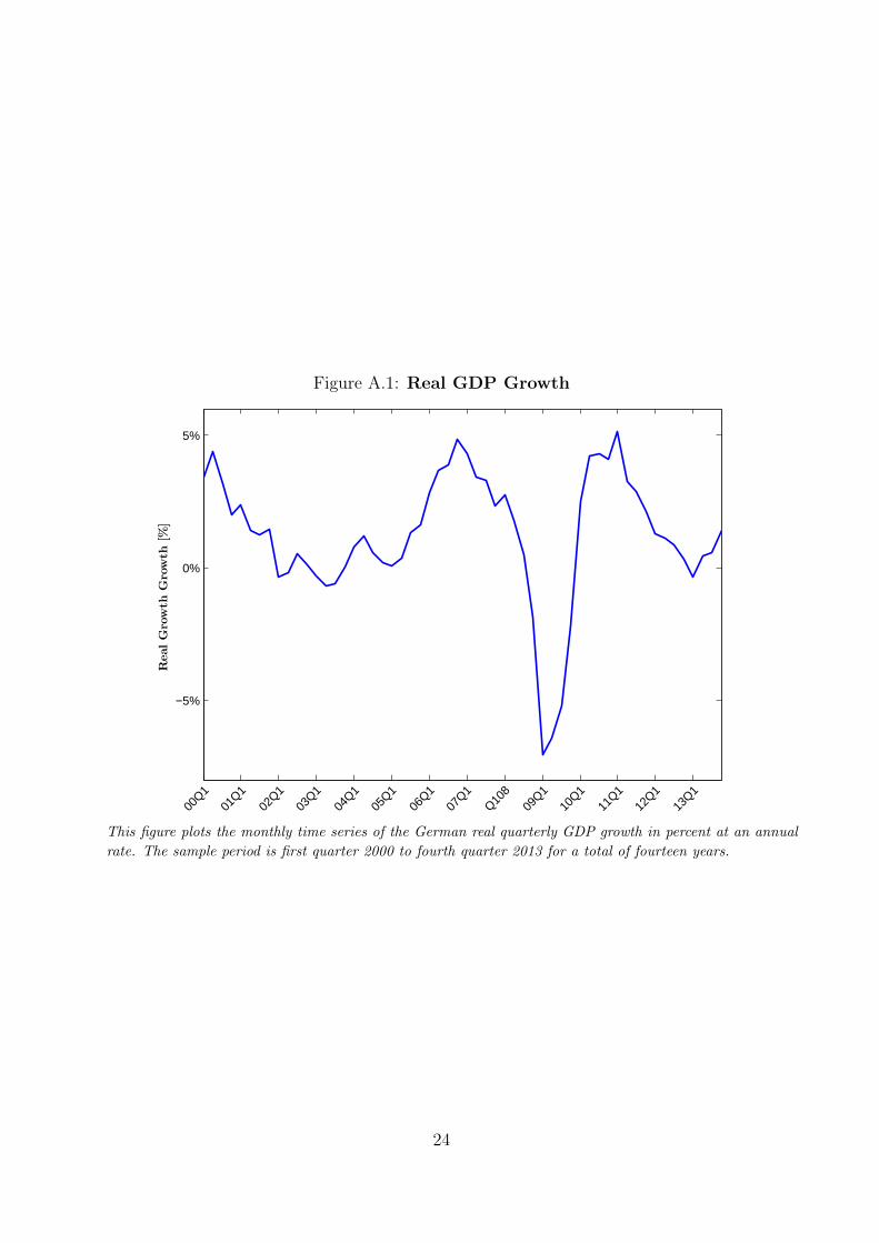
Figure A.1: Real GDP Growth

−5%

0%

5%

00Q1

01Q1

02Q1

03Q1

04Q1

05Q1

06Q1

07Q1

Q108

09Q1

10Q1

11Q1

12Q1

13Q1

RealGrowth

Growth

[%]

This figure plots the monthly time series of the German real quarterly GDP growth in percent at an annual

rate. The sample period is first quarter 2000 to fourth quarter 2013 for a total of fourteen years.

24

Figure A.2: Expected Increase in Inflation

0.1

0.2

0.3

0.4

0.5

12/0

012

/02

12/0

412

/06

12/0

812

/10

12/1

2

EU

0.1

0.2

0.3

0.4

0.5

12/0

012

/02

12/0

412

/06

12/0

812

/10

12/1

2

Germany

0.1

0.2

0.3

0.4

0.5

Fraction

Inflation

Increases

12/0

012

/02

12/0

412

/06

12/0

812

/10

12/1

2

France

0.1

0.2

0.3

0.4

0.5

Fraction

Inflation

Increases

12/0

012

/02

12/0

412

/06

12/0

812

/10

12/1

2

Austria

0.1

0.2

0.3

0.4

0.5

12/0

012

/02

12/0

412

/06

12/0

812

/10

12/1

2

Italy

0.1

0.2

0.3

0.4

0.5

12/0

012

/02

12/0

412

/06

12/0

812

/10

12/1

2

Belgium

This figure plots average monthly inflation expectations over time. We use the time series data on consumer

sentiment from the European Commission Directorate on Economic and Financial Affairs to construct these

variables. We plot the fraction of households which expects inflation to increase. The sample period is

January 2000 to December 2013 for a total of fourteen years.

25

Figure A.3: Change in the Readiness to Spend on Durables for German vs.foreign households

−0.1

−0.05

0

0.05

0.1

0.15

0.2

0.25

0.3

0.35

0.4

AverageTreatmentEffect

09/0

512

/05

03/0

606

/06

09/0

612

/06

03/0

706

/07

09/0

7

Average Treatment Effect Over TimeTwo−Standard Error Bounds

This figure plots βm coefficient (solid line) of ∆Duri,06/2005→m = α+βm×V ATshocki+∆X ′i,06/2005→m×γ+

εi and two standard deviation error bands (dashed line). ∆Duri,06/2005→m is the difference in the willingness

to spend on durable goods between month m and June 2005, V ATshocki is an indicator which equals 1 if

the household was exposed to the VAT shock, βm captures the effect of the VAT shock on the willingness

to buy durables for household i in month m, and ∆X ′i,06/2005→m is the difference in a set of observables

between month m and the baseline month. We use the micro data underlying the Directorate-General for

Economic and Financial Affairs of the European Commission harmonized consumer surveys to construct

these variables.

26

Figure A.4: Residential Property Price Inflation Rate

−4%

−3%

−2%

−1%

0%

1%

Date

RealizedHouse

PriceIn

flationRate

[%]

00Q1

01Q1

02Q1

03Q1

04Q1

05Q1

06Q1

07Q1

Q108

09Q1

10Q1

11Q1

12Q1

House Price π

This figure plots the monthly time series of the German residential property price inflation rate in percent

at an annual rate. The sample period is January 2000 to December 2013 for a total of fourteen years.

27

Figure A.5: Consensus Economics One-Year Ahead Inflation Forecast

−0.5%

0%

0.5%

1%

1.5%

2%

2.5%

00Q1

01Q1

02Q1

03Q1

04Q1

05Q1

06Q1

07Q1

Q108

09Q1

10Q1

Date

One-yearaheadIn

flationForecast

[%]

This figure plots the quarterly consensus forecasts of the one-year ahead German consumer price inflation

rate in percent at an annual rate as surveyed by Consensus Economics. The sample period is first quarter

2000 to forth quarter 2013 for a total of fourteen years.

28

Figure A.6: ZEW Financial Market Experts Inflation Forecast Index

−80

−60

−40

−20

0

20

40

60

80

12/0

012

/01

12/0

212

/03

12/0

412

/05

12/0

612

/07

12/0

812

/09

12/1

012

/11

12/1

212

/13

ZEW

InflationIndex

This figure plots the monthly time series of the ZEW inflation index for the German CPI inflation rate.

The index is the difference between the fraction of surveyed financial experts who expect inflation to increase

over the next six month minus the fraction of surveyed financial experts who expect inflation to decrease in

percent. The sample period is January 2000 to December 2013 for a total of fourteen years.

29

Figure A.7: Survey of Professional Forecasters One-Year ahead InflationForecast (Eurozone)

1%

1.5%

2%

2.5%

00Q1

01Q1

02Q1

03Q1

04Q1

05Q1

06Q1

07Q1

Q108

09Q1

10Q1

11Q1

12Q1

13Q1

Date

One-yearaheadIn

flationForecast

[%]

This figure plots the quarterly time series of the average one-year ahead forecasts by professional forecasters

for the harmonized consumer price inflation in the Eurozone in percent at an annual rate. The sample period

is first quarter 2000 to forth quarter 2013 for a total of fourteen years.

30

Figure A.8: Standardized Lagged Inflation Expectations and Change CPIInflation rate

−2

−1

0

1

2

3

4

5

StandardizedInflation

12/0

112

/02

12/0

312

/04

12/0

512

/06

12/0

712

/08

12/0

912

/10

12/1

112

/12

12/1

3

Standardized Lagged Inflation ExpectationsStandardized Change in Durable Inflation

This figure plots the monthly time series of the one-year lagged standardized average monthly inflation

expectation and the twelve months change in the harmonized major durables consumer price inflation rate

in percent at an annual rate. We use the confidential micro data underlying the GfK Consumer Climate

MAXX survey to construct inflation expectations. GfK asks a representative sample of 2,000 households how

consumer prices will evolve in the next twelve months compared to the previous twelve months. We create a

dummy variable which equals 1 when a household expects inflation to increase. The sample period is January

2001 to December 2013 for a total of thirteen years.

31

Figure A.9: Expected Decrease in Inflation

0

0.1

0.2

0.3

0.4

0.5

12/0

012

/01

12/0

212

/03

12/0

412

/05

12/0

612

/07

12/0

812

/09

12/1

012

/11

12/1

212

/13

Fraction

Inflation

Decreases

This figure plots average monthly inflation expectation over time. We use the confidential micro data

underlying the GfK Consumer Climate MAXX survey to construct this variables. GfK asks a representative

sample of 2,000 households how consumer prices will evolve in the next twelve months compared to the

previous twelve months. We create a dummy variable which equals 1 when a household expects zero or

negative inflation. The sample period is January 2000 to December 2013 for a total of fourteen years.

32

Figure A.10: Interest Rates for Consumption Loans

5.5

6.5

7.5

8.5

9.5

12/0

012

/01

12/0

212

/03

12/0

412

/05

12/0

612

/07

12/0

812

/09

12/1

012

/11

12/1

212

/13

Bank

InterestRatesfo

rConsum

ptio

nLoans[%

]

This figure plots the monthly time series of the bank interest rates for consumption loans to German

households in percent at an annual rate. The sample period is first quarter 2000 to forth quarter 2013

for a total of fourteen years.

33

Table A.1: Inflation Expectations and Readiness to Spend: Demographics andExpectations

This table reports the average marginal effects of a multinomial logit regression. Households’ readiness to purchase

durables is the dependent variable. Inflation increase is a dummy variable which equals 1 when a household

replies that inflation will increase. Past inflation measures the household perception of the increase in consumer

prices during the last twelve months. We also control for household demographics, household expectations, and

contemporaneous macroeconomic variables. We use the confidential micro data underlying the GfK Consumer

Climate MAXX survey to construct the survey variables. GfK asks a representative sample of 2,000 households on

a monthly basis whether it is a good time to purchase durables given the current economic conditions. Households

can reply that it is a good time, it is a bad time or it is neither a good time nor a bad time. Standard errors are

clustered at the quarter level. The sample period is January 2000 to December 2013 for a total of fourteen years.

Bad time Good time Bad time Good time Bad time Good time

(1) (2) (3) (4) (5) (6)

Inflation increase 0.0242∗∗∗ 0.0755∗∗∗ −0.0078 0.0888∗∗∗ 0.0051 0.0875∗∗∗(0.0094) (0.0156) (0.0083) (0.0160) (0.0073) (0.0116)

Past Inflation 0.0570∗∗∗ −0.0300∗∗∗ 0.0376∗∗∗ −0.0200∗∗∗ 0.0331∗∗∗ −0.0114∗∗∗(0.0045) (0.0030) (0.0033) (0.0035) (0.0020) (0.0023)

Sex −0.0285∗∗∗ −0.0074∗∗∗ −0.0146∗∗∗ −0.0144∗∗∗ −0.0098∗∗∗ −0.0155∗∗∗(0.0025) (0.0019) (0.0024) (0.0020) (0.0023) (0.0019)

Age 0.0018∗∗∗ −0.0008∗∗ −0.0023∗∗∗ 0.0015∗∗∗ −0.0017∗∗∗ 0.0013∗∗∗(0.0003) (0.0003) (0.0004) (0.0003) (0.0003) (0.0003)

Age2 −0.0000∗∗∗ 0.0000 0.0000∗∗∗ −0.0000∗∗∗ 0.0000∗∗∗ −0.0000∗∗∗(0.0000) (0.0000) (0.0000) (0.0000) (0.0000) (0.0000)

Education −0.0301∗∗∗ 0.0261∗∗∗ −0.0198∗∗∗ 0.0199∗∗∗ −0.0174∗∗∗ 0.0192∗∗∗(0.0016) (0.0010) (0.0016) (0.0012) (0.0017) (0.0012)

Hh size −0.0118∗∗∗ 0.0066∗∗∗ −0.0034∗∗∗ 0.0024∗∗ −0.0047∗∗∗ 0.0027∗∗(0.0012) (0.0013) (0.0011) (0.0012) (0.0012) (0.0012)

City size 0.0004 0.0006 0.0008 0.0001 0.0001 0.0004

(0.0007) (0.0005) (0.0007) (0.0006) (0.0007) (0.0006)

Marital Status 0.0091∗∗∗ −0.0026∗∗ 0.0037∗∗∗ −0.0001 0.0009 0.0003

(0.0016) (0.0013) (0.0013) (0.0012) (0.0012) (0.0011)

Kids home 0.0078 0.0027 0.0061 0.005 0.0042 0.0053

(0.0048) (0.0045) (0.0046) (0.0050) (0.0043) (0.0049)

\# kids 0.0192∗∗∗ −0.0094∗∗∗ 0.0102∗∗∗ −0.0038 0.0103∗∗∗ −0.0041

(0.0028) (0.0026) (0.0027) (0.0026) (0.0026) (0.0026)

Housing 0.0216∗∗∗ −0.0073∗∗∗ 0.0125∗∗∗ −0.0029∗∗ 0.0133∗∗∗ −0.0031∗∗∗(0.0013) (0.0012) (0.0013) (0.0012) (0.0011) (0.0012)

Job 0.0215∗∗∗ −0.0066∗∗∗ 0.0046∗∗∗ 0.0023 0.0047∗∗∗ 0.0018

(0.0017) (0.0020) (0.0014) (0.0020) (0.0013) (0.0019)

State 0.0018∗∗∗ −0.0017∗∗∗ −0.0002 −0.0008∗∗ −0.0004 −0.0008∗∗(0.0004) (0.0004) (0.0004) (0.0004) (0.0004) (0.0003)

Income −0.0147∗∗∗ 0.0084∗∗∗ −0.0079∗∗∗ 0.0047∗∗∗ −0.0070∗∗∗ 0.0044∗∗∗(0.0006) (0.0007) (0.0007) (0.0007) (0.0006) (0.0007)

Past financial situation −0.0613∗∗∗ 0.0334∗∗∗ −0.0526∗∗∗ 0.0324∗∗∗(0.0027) (0.0021) (0.0017) (0.0019)

Financial outlook −0.0236∗∗∗ 0.0215∗∗∗ −0.0192∗∗∗ 0.0206∗∗∗(0.0025) (0.0030) (0.0019) (0.0027)

Current financial situation 0.0000 −0.0008 0.0103∗∗ −0.0078∗(0.0049) (0.0037) (0.0051) (0.0041)

Exp GDP growth −0.0293∗∗∗ 0.0300∗∗∗ −0.0277∗∗∗ 0.0298∗∗∗(0.0023) (0.0025) (0.0019) (0.0022)

Exp unemployment rate 0.0315∗∗∗ −0.0024 0.0270∗∗∗ −0.0103∗∗∗(0.0028) (0.0040) (0.0014) (0.0021)

Saving propensity −0.0498∗∗∗ 0.0386∗∗∗ −0.0549∗∗∗ 0.0416∗∗∗(0.0041) (0.0028) (0.0035) (0.0025)

Good time to save 0.0067∗∗∗ −0.0279∗∗∗ 0.0004 −0.0265∗∗∗(0.0023) (0.0036) (0.0018) (0.0033)

CPI Inflation 1.4513 −4.9889∗∗(1.4110) (2.1874)

Unemployment rate −0.0076∗ 0.0165∗∗(0.0043) (0.0075)

European uncertainty 0.0000 −0.0003∗(0.0001) (0.0002)

German uncertainty −0.0002∗ 0.0004∗∗∗(0.0001) (0.0001)

Policy rate 0.0134∗ −0.0033

(0.0079) (0.0124)

Dax −0.0000∗∗∗ 0.0000

(0.0000) (0.0000)

Vdax −0.0002 0.0000

(0.0006) (0.0009)

IP growth −0.0594 −0.0207

(0.0812) (0.1170)

Oil price −0.0008∗∗∗ 0.0009∗(0.0003) (0.0005)

∆ Oil price 0.0327∗ −0.0313

(0.0172) (0.0265)

Pseudo R2 0.0292 0.0654 0.0762

Nobs 244,497 219,799 219,799

Standard errors in parentheses

∗p < 0.10, ∗ ∗ p < 0.05, ∗ ∗ ∗p < 0.01 34

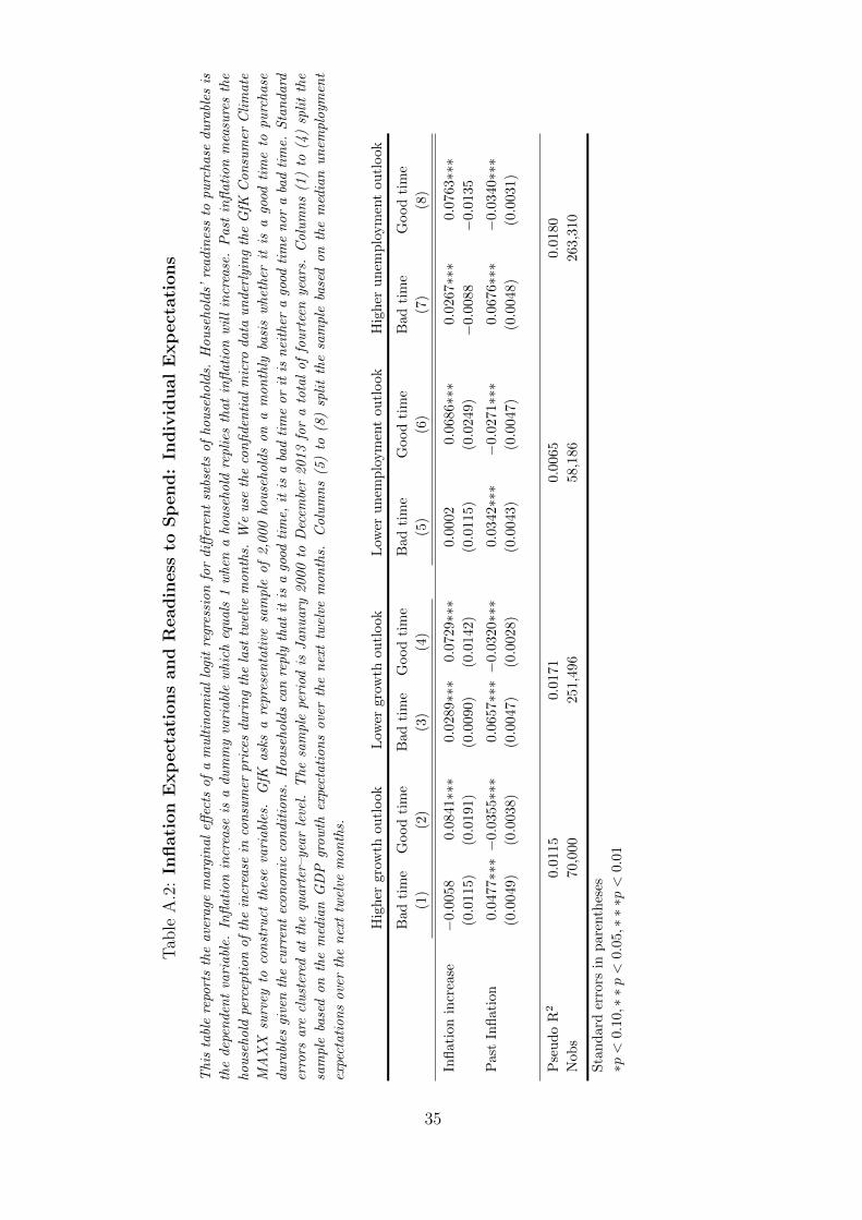
Tab

leA

.2:

Inflati

on

Exp

ect

ati

ons

and

Readin

ess

toSp

end:

Indiv

idual

Exp

ect

ati

ons

This

tabl

ere

port

sth

eave

rage

marg

inal

effec

tsof

am

ult

inom

ial

logi

tre

gres

sion

for

diff

eren

tsu

bset

sof

hou

sehold

s.H

ou

sehold

s’re

adin

ess

topu

rchase

du

rabl

esis

the

dep

enden

tva

riabl

e.In

flati

on

incr

ease

isa

du

mm

yva

riabl

ew

hic

heq

uals

1w

hen

ahou

sehold

repli

esth

at

infl

ati

on

wil

lin

crea

se.

Past

infl

ati

on

mea

sure

sth

e

hou

sehold

perc

epti

on

of

the

incr

ease

inco

nsu

mer

pri

ces

du

rin

gth

ela

sttw

elve

mon

ths.

We

use

the

con

fiden

tial

mic

rodata

un

der

lyin

gth

eG

fKC

on

sum

erC

lim

ate

MA

XX

surv

eyto

con

stru

ctth

ese

vari

abl

es.

GfK

ask

sa

repre

sen

tati

vesa

mple

of

2,0

00

hou

sehold

son

am

on

thly

basi

sw

het

her

itis

ago

odti

me

topu

rchase

du

rabl

esgi

ven

the

curr

ent

econ

om

icco

ndit

ion

s.H

ou

sehold

sca

nre

ply

that

itis

ago

odti

me,

itis

aba

dti

me

or

itis

nei

ther

ago

odti

me

nor

aba

dti

me.

Sta

ndard

erro

rsare

clu

ster

edat

the

quart

er–ye

ar

leve

l.T

he

sam

ple

peri

odis

Jan

uary

2000

toD

ecem

ber

2013

for

ato

tal

of

fou

rtee

nye

ars

.C

olu

mn

s(1

)to

(4)

spli

tth

e

sam

ple

base

don

the

med

ian

GD

Pgr

ow

thex

pect

ati

on

sove

rth

en

ext

twel

vem

on

ths.

Colu

mn

s(5

)to

(8)

spli

tth

esa

mple

base

don

the

med

ian

un

emplo

ymen

t

expe

ctati

on

sove

rth

en

ext

twel

vem

on

ths.

Hig

her

grow

thou

tlook

Low

ergro

wth

ou

tlook

Low

eru

nem

plo

ym

ent

ou

tlook

Hig

her

un

emp

loym

ent

ou

tlook

Bad

tim

eG

ood

tim

eB

ad

tim

eG

ood

tim

eB

ad

tim

eG

ood

tim

eB

ad

tim

eG

ood

tim

e

(1)

(2)

(3)

(4)

(5)

(6)

(7)

(8)

Infl

atio

nin

crea

se−

0.00

580.

0841∗∗∗

0.0289∗∗∗

0.0

729∗∗∗

0.0002

0.0686∗∗∗

0.0267∗∗∗

0.0

763∗∗∗

(0.0

115)

(0.0

191)

(0.0

090)

(0.0

142)

(0.0

115)

(0.0

249)

−0.

0088

−0.0

135

Pas

tIn

flat

ion

0.0

477∗∗∗−

0.0

355∗∗∗

0.0

657∗∗∗−

0.0

320∗∗∗

0.0342∗∗∗

−0.

0271∗∗∗

0.0676∗∗∗

−0.0

340∗∗∗

(0.0

049)

(0.0

038)

(0.0

047)

(0.0

028)

(0.0

043)

(0.0

047)

(0.0

048)

(0.0

031)

Pse

ud

oR

20.

0115

0.0

171

0.0

065

0.0

180

Nob

s70

,000

251,4

96

58,1

86

263,3

10

Sta

nd

ard

erro

rsin

par

enth

eses

∗p<

0.1

0,∗∗p<

0.05,∗∗∗p<

0.01

35

Tab

leA

.3:

Inflati

on

Exp

ect

ati

ons

and

Readin

ess

toSp

end:

Idio

syncr

ati

cE

xp

ect

ati

ons

(diff

ere

nt

cuto

ff)

This

tabl

ere

port

sth

eave

rage

marg

inal

effec

tsof

am

ult

inom

ial

logi

tre

gres

sion

for

diff

eren

tsu

bset

sof

hou

sehold

s.H

ou

sehold

s’re

adin

ess

topu

rchase

du

rabl

es

isth

edep

enden

tva

riabl

e.In

flati

on

incr

ease

isa

du

mm

yva

riabl

ew

hic

heq

uals

1w

hen

ahou

sehold

repli

esth

at

infl

ati

on

wil

lin

crea

se.

Past

infl

ati

on

mea

sure

s

the

hou

sehold

perc

epti

on

of

the

incr

ease

inco

nsu

mer

pri

ces

du

rin

gth

ela

sttw

elve

mon

ths.

We

use

the

con

fiden

tial

mic

rodata

un

der

lyin

gth

eG

fKC

on

sum

er

Cli

mate

MA

XX

surv

eyto

con

stru

ctth

ese

vari

abl

es.

GfK

ask

sa

repre

sen

tati

vesa

mple

of

2,0

00

hou

sehold

son

am

on

thly

basi

sw

het

her

itis

ago

odti

me

to

pu

rchase

du

rabl

esgi

ven

the

curr

ent

econ

om

icco

ndit

ion

s.H

ou

sehold

sca

nre

ply

that

itis

ago

odti

me,

itis

aba

dti

me,

or

itis

nei

ther

ago

odti

me

nor

aba

d

tim

e.S

tan

dard

erro

rsare

clu

ster

edat

the

quart

erle

vel.

The

sam

ple

peri

odis

Jan

uary

2000

toD

ecem

ber

2013

for

ato

tal

of

fou

rtee

nye

ars

.W

eass

ign

med

ian

obs

erva

tion

sto

the

posi

tive

expe

ctati

on

sam

ple

.C

olu

mn

s(1

)to

(4)

spli

tth

esa

mple

base

don

the

med

ian

perc

epti

on

of

hou

sehold

s’fi

nan

cial

situ

ati

on

ove

rth

e

last

twel

vem

on

ths.

Colu

mn

(5)

to(8

)sp

lit

the

sam

ple

base

don

the

med

ian

expe

ctati

on

of

hou

sehold

s’fi

nan

cial

situ

ati

on

ove

rth

en

ext

twel

vem

on

ths.

Pos

itiv

efi

nan

cial

per

cep

tion

Neg

ati

vefi

nan

cial

per

cep

tion

Posi

tive

fin

an

cial

exp

ecta

tion

Neg

ati

vefi

nan

cial

exp

ecta

tion

Bad

tim

eG

ood

tim

eB

ad

tim

eG

ood

tim

eB

ad

tim

eG

ood

tim

eB

ad

tim

eG

ood

tim

e

(1)

(2)

(3)

(4)

(5)

(6)

(7)

(8)

Infl

atio

nin

crea

se0.0

066

0.0

880∗∗∗

0.0328∗∗

0.0498∗∗∗

−0.0

013

0.0841∗∗∗

0.0138

0.0

624∗∗∗

(0.0

073)

(0.0

156)

(0.0

144)

(0.0

145)

(0.0

075)

(0.0

141)

(0.0

184)

(0.0

193)

Pas

tIn

flat

ion

0.0

360∗∗∗

−0.0

256∗∗∗

0.0737∗∗∗

−0.

0362∗∗∗

0.0

504∗∗∗

−0.

0301∗∗∗

0.0767∗∗∗

−0.0

401∗∗∗

(0.0

029)

(0.0

029)

(0.0

049)

(0.0

034)

(0.0

044)

(0.0

028)

(0.0

052)

(0.0

042)

Pse

ud

oR

20.

0087

0.0

162

0.0

121

0.0

179

Nob

s23

7,78

483,7

12

274,4

44

47,0

52

Sta

nd

ard

erro

rsin

par

enth

eses

∗p<

0.1

0,∗∗p<

0.05,∗∗∗p<

0.01

36

Tab

leA

.4:

Inflati

on

Exp

ect

ati

ons

and

Readin

ess

toSp

end:

Indiv

idual

Exp

ect

ati

ons

(diff

ere

nt

cuto

ff)

This

tabl

ere

port

sth

eave

rage

marg

inal

effec

tsof

am

ult

inom

ial

logi

tre

gres

sion

for

diff

eren

tsu

bset

sof

hou

sehold

s.H

ou

sehold

s’re

adin

ess

topu

rchase

du

rabl

esis

the

dep

enden

tva

riabl

e.In

flati

on

incr

ease

isa

du

mm

yva

riabl

ew

hic

heq

uals

1w

hen

ahou

sehold

repli

esth

at

infl

ati

on

wil

lin

crea

se.

Past

infl

ati

on

mea

sure

sth

e

hou

sehold

perc

epti

on

of

the

incr

ease

inco

nsu

mer

pri

ces

du

rin

gth

ela

sttw

elve

mon

ths.

We

use

the

con

fiden

tial

mic

rodata

un

der

lyin

gth

eG

fKC

on

sum

erC

lim

ate

MA

XX

surv

eyto

con

stru

ctth

ese

vari

abl

es.

GfK

ask

sa

repre

sen

tati

vesa

mple

of

2,0

00

hou

sehold

son

am

on

thly

basi

sw

het

her

itis

ago

odti

me

topu

rchase

du

rabl

esgi

ven

the

curr

ent

econ

om

icco

ndit

ion

s.H

ou

sehold

sca

nre

ply

that

itis

ago

odti

me,

itis

aba

dti

me,

or

itis

nei

ther

ago

odti

me

nor

aba

dti

me.

Sta

ndard

erro

rsare

clu

ster

edat

the

quart

erle

vel.

The

sam

ple

peri

odis

Jan

uary

2000

toD

ecem

ber

2013

for

ato

tal

of

fou

rtee

nye

ars

.W

eass

ign

med

ian

obs

erva

tion

sto

the

posi

tive

expe

ctati

on

sam

ple

.C

olu

mn

s(1

)to

(4)

spli

tth

esa

mple

base

don

the

med

ian

GD

Pgr

ow

thex

pect

ati

on

sove

rth

en

ext

twel

vem

on

ths.

Colu

mn

s(5

)

to(8

)sp

lit

the

sam

ple

base

don

the

med

ian

un

emplo

ymen

tex

pect

ati

on

sove

rth

en

ext

twel

vem

on

ths.

Hig

her

grow

thou

tlook

Low

ergro

wth

ou

tlook

Low

eru

nem

plo

ym

ent

ou

tlook

Hig

her

un

emp

loym

ent

ou

tlook

Bad

tim

eG

ood

tim

eB

ad

tim

eG

ood

tim

eB

ad

tim

eG

ood

tim

eB

ad

tim

eG

ood

tim

e

(1)

(2)

(3)

(4)

(5)

(6)

(7)

(8)

Infl

atio

nin

crea

se−

0.00

680.

0953∗∗∗

0.02

0.0609∗∗∗

−0.

0046

0.0879∗∗∗

0.0283∗∗∗

0.0

671∗∗∗

(0.0

088)

(0.0

161)

(0.0

122)

(0.0

138)

(0.0

096)

(0.0

204)

(0.0

091)

(0.0

114)

Pas

tIn

flat

ion

0.0

453∗∗∗−

0.0

250∗∗∗

0.0

721∗∗∗−

0.0

414∗∗∗

0.0426∗∗∗

−0.

0221∗∗∗

0.0739∗∗∗

−0.0

435∗∗∗

(0.0

047)

(0.0

030)

(0.0

048)

(0.0

035)

(0.0

042)

(0.0

030)

(0.0

050)

(0.0

035)

Pse

ud

oR

20.

0108

0.0

178

0.0

098

0.0

198

Nob

s21

1,49

9109,9

97

169,2

73

152,2

23

Sta

nd

ard

erro

rsin

par

enth

eses

∗p<

0.1

0,∗∗p<

0.05,∗∗∗p<

0.01

37

Table A.5: Inflation Expectations and Readiness to Spend: Inflation dummiesand OLS

This table reports the average marginal effects of a multinomial logit regression for different time periods.

Households’ readiness to purchase durables is the dependent variable. Inflation expectation is a dummy variable

which equals 1 when a household replies that inflation will increase. Past inflation measures the household perception

of the increase in consumer prices during the last twelve months. We also control for household demographics and

household expectations. We use the confidential micro data underlying the GfK Consumer Climate MAXX survey

to construct these variables. GfK asks a representative sample of 2,000 households on a monthly basis whether it

is a good time to purchase durables given the current economic conditions. Households can reply that it is a good

time, it is a bad time, or it is neither a good time nor a bad time. Standard errors are clustered at the quarter

level. The sample period is January 2000 to December 2013 for a total of fourteen years. Columns (1) and (2)

add dummy variables for past inflation, columns (3) and (4) add dummy variables for inflation expectations, and

column (5) estimates an OLS specification.

Past inflation dummies Inflation expectation dummies OLS

Bad time Good time Bad time Good time

(1) (2) (3) (4) (5)

Inflation increase −0.0072 0.0874∗∗∗ 0.0988∗∗∗(0.0081) (0.0161) (0.0272)

Prices will increase less −0.0167∗∗∗ 0.0234∗∗∗(0.0047) (0.0061)

Prices will increase the same −0.0295∗∗∗ 0.0202∗∗∗(0.0060) (0.0073)

Prices will increase more −0.0292∗∗∗ 0.1048∗∗∗(0.0109) (0.0193)

Past Inflation 0.0419∗∗∗ −0.0237∗∗∗ −0.0598∗∗∗(0.0034) (0.0034) (0.0061)

Prices stayed constant −0.0164 −0.1497∗∗∗(0.0140) (0.0115)

Prices increased slightly −0.0039 −0.1574∗∗∗(0.0164) (0.0129)

Prices increased somewhat 0.0164 −0.1585∗∗∗(0.0172) (0.0136)

Prices increased substantially 0.0919∗∗∗ −0.1953∗∗∗(0.0184) (0.0143)

Demographics X X X X X

Individual expectations X X X X X

Pseudo R2 0.0676 0.0657 0.1056

Nobs 219,799 215,579 219,799

Standard errors in parentheses

∗p < 0.10, ∗ ∗ p < 0.05, ∗ ∗ ∗p < 0.01

38

Tab

leA

.6:

Inflati

on

Exp

ect

ati

ons

and

Readin

ess

toSp

end:

month

&year

dum

mie

sand

ord

ere

dpro

bit

This

tabl

ere

port

sth

eave

rage

marg

inal

effec

tsof

mu

ltin

om

ial

logi

tan

dord

ered

pro

bit

regr

essi

on

sfo

rdiff

eren

tti

me

peri

ods.

Hou

sehold

s’re

adin

ess

topu

rchase

du

rabl

esis

the

dep

enden

tva

riabl

e.In

flati

on

expe

ctati

on

isa

du

mm

yva

riabl

ew

hic

heq

uals

1w

hen

ahou

sehold

repli

esth

at

infl

ati

on

wil

lin

crea

se.

Past

infl

ati

on

mea

sure

sth

ehou

sehold

perc

epti

on

of

the

incr

ease

inco

nsu

mer

pri

ces

du

rin

gth

ela

sttw

elve

mon

ths.

We

als

oco

ntr

ol

for

hou

sehold

dem

ogra

phic

san

dhou

sehold

expe

ctati

on

s.W

eu

seth

eco

nfi

den

tial

mic

rodata

un

der

lyin

gth

eG

fKC

on

sum

erC

lim

ate

MA

XX

surv

eyto

con

stru

ctth

ese

vari

abl

es.

GfK

ask

sa

repre

sen

tati

ve

sam

ple

of

2,0

00

hou

seho

lds

on

am

on

thly

basi

sw

het

her

itis

ago

odti

me

topu

rchase

du

rabl

esgi

ven

the

curr

ent

econ

om

icco

ndit

ion

s.H

ou

sehold

sca

nre

ply

that

itis

ago

odti

me,

itis

aba

dti

me,

or

itis

nei

ther

ago

odti

me

nor

aba

dti

me.

Sta

ndard

erro

rsare

clu

ster

edat

the

quart

erle

vel.

The

sam

ple

peri

odis

Jan

uary

2000

toD

ecem

ber

2013

for

ato

tal

of

fou

rtee

nye

ars

.C

olu

mn

s(1

)an

d(2

)re

stri

ctth

esa

mple

to2006

tost

udy

the

effec

tof

the

un

expe

cted

VA

Tin

crea

sein

2007,

colu

mn

s(3

)an

d(4

)ex

clu

de

2006,

an

dco

lum

ns

(5)

an

d(6

)re

stri

ctth

esa

mple

to2010

to2012

tost

udy

the

effec

tof

the

Eu

rope

an

sove

reig

ndeb

tcr

isis

.

Mon

thd

um

mie

sY

ear

du

mm

ies

Ord

ered

pro

bit

No

past

infl

ati

on

Bad

tim

eG

ood

tim

eB

ad

tim

eG

ood

tim

eB

ad

tim

eG

ood

tim

eB

ad

tim

eG

ood

tim

e

(1)

(2)

(3)

(4)

(5)

(6)

(7)

(8)

Infl

atio

nin

crea

se−

0.0

074

0.08

78∗∗∗

0.0139∗∗∗

0.0719∗∗∗

−0.

0504∗∗∗

0.0479∗∗∗

0.0048

0.0827∗∗∗

(0.0

081)

(0.0

151)

(0.0

051)

(0.0

070)

(0.0

137)

(0.0

139)

(0.0

095)

(0.0

167)

Pas

tIn

flat

ion

0.0

376∗∗∗−

0.0

200∗∗∗

0.0

309∗∗∗−

0.0096∗∗∗

0.0307∗∗∗−

0.0291∗∗∗

(0.0

033)

(0.0

035)

(0.0

015)

(0.0

026)

(0.0

033)

(0.0

029)

Dem

ogra

ph

ics

XX

XX

XX

XX

Ind

ivid

ual

exp

ecta

tion

sX

XX

XX

XX

X

Pse

ud

oR

20.

0657

0.0

819

0.0

564

0.0

603

Nob

s21

9,79

9219,7

99

219,7

99

221,3

92

Sta

nd

ard

erro

rsin

par

enth

eses

∗p<

0.1

0,∗∗p<

0.05,∗∗∗p<

0.01

39

Table A.7: Inflation Expectations and Readiness to Save

This table reports the average marginal effects of a multinomial logit regression. Households’ readiness to save is

the dependent variable. Inflation expectation is a dummy variable which equals 1 when a households replies that

inflation will increase. Past inflation measures the household perception of the increase in consumer prices during

the last twelve months. We use the confidential micro data underlying the GfK Consumer Climate MAXX survey

to construct these variables. GfK asks a representative sample of 2,000 households on a monthly basis whether it

is a good time to purchase durables given the current economic conditions. Households can reply that it is a good

time, it is probably a good time, it is not really a good time, or it is not at all a good time. Standard errors are

clustered at the quarter level. The sample period is January 2000 to December 2013 for a total of fourteen years.

Not at all Not really Good time

(1) (2) (3)

Inflation increase 0.0160∗∗∗ 0.0082∗∗ 0.0006

(0.0016) (0.0036) (0.0082)

Past Inflation 0.0019∗∗ −0.0134∗∗∗ 0.0332∗∗∗(0.0007) (0.0023) (0.0045)

Demographics X X X

Individual expectations X X X

Pseudo R2 0.0203

Nobs 234,522

Standard errors in parentheses

∗p < 0.10, ∗ ∗ p < 0.05, ∗ ∗ ∗p < 0.01

40

Tab

leA

.8:

Inflati

on

Exp

ect

ati

ons

and

Readin

ess

toSp

end:

Dura

ble

Sub-c

ate

gori

es

This

tabl

ere

port

sth

eave

rage

marg

inal

effec

tsof

am

ult

inom

ial

logi

tre

gres

sion

for

diff

eren

tci

tysi

zes.

Hou

sehold

ssp

endin

gm

ore

on

diff

eren

tdu

rabl

esin

the

nex

ttw

elve

mon

ths

com

pare

dto

the

pre

viou

stw

elve

mon

ths

isth

edep

enden

tva

riabl

e.In

flati

on

incr

ease

isa

du

mm

yva

riabl

ew

hic

heq

uals

1w

hen

ahou

sehold

s

repli

esth

at

infl

ati

on

wil

lin

crea

se.

Past

infl

ati

on

mea

sure

sth

eh

ou

sehold

perc

epti

on

of

the

incr

ease

inco

nsu

mer

pri

ces

du

rin

gth

ela

sttw

elve

mon

ths.

We

als

o

con

trol

for

hou

seh

old

dem

ogra

phic

san

dhou

sehold

expe

ctati

on

s.W

eu

seth

eco

nfi

den

tial

mic

rod

ata

un

der

lyin

gth

eG

fKC

on

sum

erC

lim

ate

MA

XX

surv

eyto

con

stru

ctth

ese

vari

abl

es.

GfK

ask

sa

repre

sen

tati

vesa

mple

of

2,0

00

hou

sehold

son

aqu

art

erly

basi

sw

het

her

hou

sehold

sw

an

tto

spen

dm

ore

on

cert

ain

good

s

inth

en

ext

twel

vem

on

ths

com

pare

dto

the

pre

viou

stw

elve

mon

ths.

Hou

sehold

sca

nre

ply

that

they

wan

tto

spen

dm

ore

,th

esa

me,

or

less

.S

tan

dard

erro

rs

are

clu

ster

edat

the

quart

erle

vel.

The

sam

ple

peri

odis

firs

tqu

art

er2000

tofo

urt

hqu

art

er2013

for

ato

tal

of

fou

rtee

nye

ars

.C

olu

mn

s(1

)an

d(2

)st

udy

the

pro

pen

sity

tobu

yca

rs,

colu

mn

s(3

)an

d(4

)st

udy

the

pro

pen

sity

tore

nova

te,

colu

mn

s(5

)an

d(6

)st

udy

the

pro

pen

sity

tobu

yhou

sehold

appli

an

ces,

an

dco

lum

ns

(7)

an

d(8

)st

udy

the

pro

pen

sity

topu

rchase

furn

itu

re.

Car

Ren

ovate

Ap

pli

an

ces

Fu

rnit

ure

Bad

tim

eG

ood

tim

eB

ad

tim

eG

ood

tim

eB

ad

tim

eG

ood

tim

eB

ad

tim

eG

ood

tim

e

(1)

(2)

(3)

(4)

(5)

(6)

(7)

(8)

Infl

atio

nIn

crea

se−

0.0

012

0.02

65∗∗∗

−0.

0177∗∗∗

0.0234∗∗∗

−0.

0134∗∗

0.0185∗∗∗

−0.

0245∗∗∗

0.0179∗∗∗

(0.0

061)

(0.0

031)

(0.0

061)

(0.0

044)

(0.0

058)

(0.0

024)

(0.0

061)

(0.0

033)

Pas

tIn

flat

ion

0.0

055∗

0.0

040∗∗

0.0

116∗∗∗

0.0088∗∗∗

0.0232∗∗∗−

0.0012

0.0227∗∗∗

0.0026∗

(0.0

033)

(0.0

016)

(0.0

032)

(0.0

021)

(0.0

027)

(0.0

008)

(0.0

028)

(0.0

015)

Dem

ogra

ph

ics

XX

XX

XX

XX

Ind

ivid

ual

exp

ecta

tion

sX

XX

XX

XX

X

Pse

ud

oR

20.

0393

0.0

225

0.0

377

0.0

378

Nob

s59

,011

57,6

55

71,6

99

69,0

13

Sta

nd

ard

erro

rsin

par

enth

eses

∗p<

0.1

0,∗∗p<

0.05,∗∗∗p<

0.01

41

Table A.9: Deflation Expectations and Readiness to Spend

This table reports the average marginal effects of a multinomial logit regression. Households’ readiness to purchase

durables is the dependent variable. Deflation is a dummy variable which equals 1 when a household replies that

inflation will be zero or negative. Past inflation measures the household perception of the increase in consumer

prices during the last twelve months. We use the confidential micro data underlying the GfK Consumer Climate

MAXX survey to construct these variables. GfK asks a representative sample of 2,000 households on a monthly

basis whether it is a good time to purchase durables given the current economic conditions. Households can reply

that it is a good time, it is a bad time, or it is neither a good time nor a bad time. Standard errors are clustered

at the quarter level. The sample period is January 2000 to December 2013 for a total of fourteen years.

Bad time Good time

(1) (2)

Deflation 0.0265∗∗∗ −0.0355∗∗∗(0.0059) (0.0096)

Past Inflation 0.0414∗∗∗ −0.0225∗∗∗(0.0034) (0.0035)

Demographics X X

Individual expectations X X

Pseudo R2 0.0628

Nobs 219,799

Standard errors in parentheses

∗p < 0.10, ∗ ∗ p < 0.05, ∗ ∗ ∗p < 0.01

42

Tab

leA

.10:

Inflati

on

Exp

ect

ati

ons

and

Readin

ess

toSp

end:

House

hold

Siz

e

This

tabl

ere

port

sth

eave

rage

marg

inal

effec

tsof

am

ult

inom

ial

logi

tre

gres

sion

for

diff

eren

thou

sehold

ssi

zes.

Hou

sehold

s’re

adin

ess

topu

rchase

du

rabl

esis

the

dep

enden

tva

riabl

e.In

flati

on

incr

ease

isa

du

mm

yva

riabl

ew

hic

heq

uals

1w

hen

ahou

sehold

repli

esth

at

infl

ati

on

wil

lin

crea

se.

Past

infl

ati

on

mea

sure

sth

e

hou

sehold

perc

epti

on

of

the

incr

ease

inco

nsu

mer

pri

ces

du

rin

gth

ela

sttw

elve

mon

ths.

We

als

oco

ntr

ol

for

hou

sehold

dem

ogra

phic

san

dhou

sehold

expe

ctati

on

s.

We

use

the

con

fiden

tial

mic

rodata

un

der

lyin

gth

eG

fKC

on

sum

erC

lim

ate

MA

XX

surv

eyto

con

stru

ctth

ese

vari

abl

es.

GfK

ask

sa

repre

sen

tati

vesa

mple

of

2,0

00

hou

sehold

son

am

on

thly

basi

sw

het

her

itis

ago

odti

me

topu

rchase

du

rabl

esgi

ven

the

curr

ent

econ

om

icco

ndit

ion

s.H

ou

sehold

sca

nre

ply

that

itis

ago

odti

me,

itis

aba

dti

me,

or

itis

nei

ther

ago

odti

me

nor

aba

dti

me.

Sta

ndard

erro

rsare

clu

ster

edat

the

quart

erle

vel.

The

sam

ple

peri

odis

Jan

uary

2000

toD

ecem

ber

2013

for

ato

tal

of

fou

rtee

nye

ars

.C

olu

mn

s(1

)an

d(2

)re

stri

ctth

esa

mple

tore

spon

den

tsli

vin

gin

ahou

sehold

of

size

1,

colu

mn

s(3

)an

d(4

)to

resp

on

den

ts

livi

ng

ina

hou

sehold

of

size

2,

colu

mn

s(5

)an

d(6

)to

resp

on

den

tsli

vin

gin

ahou

sehold

of

size

3,

colu

mn

s(7

)an

d(8

)to

resp

on

den

tsli

vin

gin

ahou

sehold

of

size

4,

an

dco

lum

ns

(9)

an

d(1

0)

tore

spon

den

tsbe

twee

nli

vin

gin

ahou

sehold

of

size

5.

Hou

seh

old

size

:1

Hou

seh

old

size

:2

Hou

seh

old

size

:3

Hou

seh

old

size

:4

House

hold

size

:5

Bad

tim

eG

ood

tim

eB

ad

tim

eG

ood

tim

eB

ad

tim

eG

ood

tim

eB

ad

tim

eG

ood

tim

eB

ad

tim

eG

ood

tim

e

(1)

(2)

(3)

(4)

(5)

(6)

(7)

(8)

(9)

(10)

Infl

ati

on

incr

ease

−0.0

064

0.0

820∗∗∗

−0.0

098

0.0

881∗∗∗

−0.0

107

0.0

874∗∗∗

−0.0

051

0.0

998∗∗∗

0.0

009

0.0

946∗∗∗

(0.0

090)

(0.0

157)

(0.0

096)

(0.0

164)

(0.0

096)

(0.0

167)

(0.0

090)

(0.0

171)

(0.0

144)

(0.0

210)

Past

Infl

ati

on

0.0

426∗∗∗−

0.0

198∗∗∗

0.0

366∗∗∗−

0.0

205∗∗∗

0.0

369∗∗∗−

0.0

209∗∗∗

0.0

350∗∗∗−

0.0

179∗∗∗

0.0

351∗∗∗−

0.0

221∗∗∗

(0.0

036)

(0.0

036)

(0.0

033)

(0.0

036)

(0.0

040)

(0.0

045)

(0.0

034)

(0.0

039)

(0.0

056)

(0.0

045)

Dem

ogra

ph

ics

XX

XX

XX

XX

XX

Ind

ivid

ual

exp

ecta

tion

sX

XX

XX

XX

XX

X

Pse

ud

oR

20.0

662

0.0

657

0.0

658

0.0

691

0.0

632

Nob

s50,0

27

82,0

26

41,9

09

34,1

03

11,7

34

Sta

nd

ard

erro

rsin

pare

nth

eses

∗p<

0.1

0,∗∗p<

0.0

5,∗∗∗p<

0.0

1

43

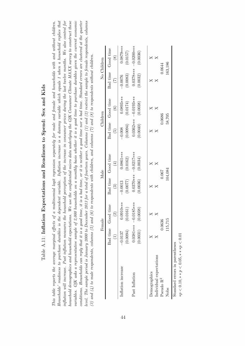
Tab

leA

.11:

Inflati

on

Exp

ect

ati

ons

and

Readin

ess

toSp

end:

Sex

and

Kid

s

This

tabl

ere

port

sth

eave

rage

marg

inal

effec

tsof

am

ult

inom

ial

logi

tre

gres

sion

sepa

rate

lyfo

rm

ale

an

dfe

male

an

dhou

sehold

sw

ith

an

dw

ithou

tch

ildre

n.

Hou

sehold

s’re

adin

ess

topu

rchase

du

rabl

esis

the

dep

enden

tva

riabl

e.In

flati

on

incr

ease

isa

du

mm

yva

riabl

ew

hic

heq

uals

1w

hen

ahou

sehold

repli

esth

at

infl

ati

on

wil

lin

crea

se.

Past

infl

ati

on

mea

sure

sth

ehou

sehold

perc

epti

on

of

the

incr

ease

inco

nsu

mer

pri

ces

du

rin

gth

ela

sttw

elve

mon

ths.

We

als

oco

ntr

ol

for

hou

sehold

dem

ogra

phic

san

dhou

sehold

expe

ctati

on

s.W

eu

seth

eco

nfi

den

tial

mic

rodata

un

der

lyin

gth

eG

fKC

on

sum

erC

lim

ate

MA

XX

surv

eyto

con

stru

ctth

ese

vari

abl

es.

GfK

ask

sa

repre

sen

tati

vesa

mple

of

2,0

00

hou

sehold

son

am

on

thly

basi

sw

het

her

itis

ago

odti

me

topu

rchase

du

rabl

esgi

ven

the

curr

ent

econ

om

ic

con

dit

ion

s.H

ou

sehold

sca

nre

ply

that

itis

ago

odti

me,

itis

aba

dti

me,

or

itis

nei

ther

ago

odti

me

nor

aba

dti

me.

Sta

ndard

erro

rsare

clu

ster

edat

the

quart

er

leve

l.T

he

sam

ple

peri

odis

Jan

uary

2000

toD

ecem

ber

2013

for

ato

tal

of

fou

rtee

nye

ars

.C

olu

mn

s(1

)an

d(2

)re

stri

ctth

esa

mple

tofe

male

resp

on

den

ts,

colu

mn

s

(3)

an

d(4

)to

male

resp

on

den

ts,

colu

mn

s(5

)an

d(6

)to

resp

on

den

tsw

ith

chil

dre

n,

an

dco

lum

ns

(7)

an

d(8

)to

resp

on

den

tsw

ithou

tch

ildre

n.

Fem

ale

Male

Ch

ild

ren

No

Ch

ild

ren

Bad

tim

eG

ood

tim

eB

ad

tim

eG

ood

tim

eB

ad

tim

eG

ood

tim

eB

ad

tim

eG

ood

tim

e

(1)

(2)

(3)

(4)

(5)

(6)

(7)

(8)

Infl

atio

nin

crea

se−

0.01

370.

0910∗∗∗

−0.

0013

0.0861∗∗∗

−0.

008

0.0893∗∗∗

−0.

0076

0.0879∗∗∗

(0.0

094)

(0.0

161)

(0.0

077)

(0.0

162)

(0.0

094)

(0.0

174)

(0.0

083)

(0.0

157)

Pas

tIn

flat

ion

0.0

381∗∗∗−

0.0

185∗∗∗

0.0

370∗∗∗−

0.0

217∗∗∗

0.0

362∗∗∗−

0.0

193∗∗∗

0.0

378∗∗∗−

0.0

200∗∗∗

(0.0

031)

(0.0

038)

(0.0

036)

(0.0

034)

(0.0

040)

(0.0

038)

(0.0

032)

(0.0

036)

Dem

ogra

ph

ics

XX

XX

XX

XX

Ind

ivid

ual

exp

ecta

tion

sX

XX

XX

XX

X

Pse

ud

oR

20.

0636

0.0

67

0.0

686

0.0

644

Nob

s11

5,71

5104,0

84

58,7

05

163,1

86

Sta

nd

ard

erro

rsin

par

enth

eses

∗p<

0.10,∗∗p<

0.0

5,∗∗∗p<

0.01

44

Tab

leA

.12:

Inflati

on

Exp

ect

ati

ons

and

Readin

ess

toSp

end:

Mari

tal

Sta

tus

This

tabl

ere

port

sth

eave

rage

marg

inal

effec

tsof

am

ult

inom

ial

logi

tre

gres

sion

bym

ari

tal

statu

s.H

ou

sehold

s’re

adin

ess

topu

rchase

du

rabl

esis

the

dep

enden

t

vari

abl

e.In

flati

on

incr

ease

isa

du

mm

yva

riabl

ew

hic

heq

uals

1w

hen

ahou

sehold

repli

esth

at

infl

ati

on

wil

lin

crea

se.

Past

infl

ati

on

mea

sure

sth

ehou

sehold

perc

epti

on

of

the

incr

ease

inco

nsu

mer

pri

ces

du

rin

gth

ela

sttw

elve

mon

ths.

We

als

oco

ntr

ol

for

hou

sehold

dem

ogra

phic

san

dhou

sehold

expe

ctati

on

s.W

eu

seth

e

con

fiden

tial

mic

rodata

un

der

lyin

gth

eG

fKC

on

sum

erC

lim

ate

MA

XX

surv

eyto

con

stru

ctth

ese

vari

abl

es.

GfK

ask

sa

repre

sen

tati

vesa

mple

of

2,0

00

hou

sehold

s

on

am

on

thly

basi

sw

het

her

itis

ago

odti

me

topu

rchase

du

rabl

esgi

ven

the

curr

ent

econ

om

icco

ndit

ion

s.H

ou

sehold

sca

nre

ply

that

itis

ago

odti

me,

itis

aba

d

tim

e,or

itis

nei

ther

ago

odti

me

nor

aba

dti

me.

Sta

ndard

erro

rsare

clu

ster

edat

the

quart

erle

vel.

The

sam

ple

peri

odis

Jan

uary

2000

toD

ecem

ber

2013

for

ato

tal

of

fou

rtee

nye

ars

.C

olu

mn

s(1

)an

d(2

)re

stri

ctth

esa

mple

tosi

ngl

ere

spon

den

ts,

colu

mn

s(3

)an

d(4

)to

resp

on

den

tsin

are

lati

on

ship

,co

lum

ns

(5)

an

d

(6)

tom

arr

ied

resp

on

den

ts,

an

dco

lum

ns

(7)

an

d(8

)to

div

orc

edre

spon

den

ts.

Sin

gle

Cou

ple

Marr

ied

Div

orc

ed

Bad

tim

eG

ood

tim

eB

ad

tim

eG

ood

tim

eB

ad

tim

eG

ood

tim

eB

ad

tim

eG

ood

tim

e

(1)

(2)

(3)

(4)

(5)

(6)

(7)

(8)

Infl

atio

nin

crea

se−

0.0

147

0.09

05∗∗∗

−0.

0171

0.0824∗∗∗

−0.

0021

0.0925∗∗∗

−0.

0122

0.0777∗∗∗

(0.0

093)

(0.0

177)

(0.0

113)

(0.0

179)

(0.0

085)

(0.0

157)

(0.0

111)

(0.0

157)

Pas

tIn

flat

ion

0.0

385∗∗∗−

0.0

218∗∗∗

0.0

356∗∗∗−

0.0173∗∗∗

0.0354∗∗∗−

0.0210∗∗∗

0.0442∗∗∗−

0.0177∗∗∗

(0.0

040)

(0.0

042)

(0.0

046)

(0.0

047)

(0.0

030)

(0.0

037)

(0.0

041)

(0.0

034)

Dem

ogra

ph

ics

XX

XX

XX

XX

Ind

ivid

ual

exp

ecta

tion

sX

XX

XX

XX

X

Pse

ud

oR

20.

0575

0.0

695

0.0

678

0.0

677

Nob

s46

,701

25,0

08

111,7

60

36,3

30

Sta

nd

ard

erro

rsin

par

enth

eses

∗p<

0.1

0,∗∗p<

0.05,∗∗∗p<

0.01

45

Table A.13: Inflation Expectations and Readiness to Spend: Homeownership

This table reports the average marginal effects of a multinomial logit regression by home ownership. Households’

readiness to purchase durables is the dependent variable. Inflation increase is a dummy variable which equals 1 when

a household replies that inflation will increase. Past inflation measures the household perception of the increase

in consumer prices during the last twelve months. We also control for household demographics and household

expectations. We use the confidential micro data underlying the GfK Consumer Climate MAXX survey to construct

these variables. GfK asks a representative sample of 2,000 households on a monthly basis whether it is a good time

to purchase durables given the current economic conditions. Households can reply that it is a good time, it is a bad

time, or it is neither a good time nor a bad time. Standard errors are clustered at the quarter level. The sample

period is January 2000 to December 2013 for a total of fourteen years. Columns (1) and (2) restrict the sample to

home owners, columns (3) and (4) to apartment owners, and columns (5) and (6) to renters.

House owner Apartment owner Renter

Bad time Good time Bad time Good time Bad time Good time

(1) (2) (3) (4) (5) (6)

Inflation increase −0.0038 0.0834∗∗∗ −0.0115 0.0766∗∗∗ −0.0105 0.0938∗∗∗(0.0080) (0.0173) (0.0120) (0.0191) (0.0096) (0.0156)

Past Inflation 0.0342∗∗∗ −0.0216∗∗∗ 0.0306∗∗∗ −0.0228∗∗∗ 0.0410∗∗∗ −0.0186∗∗∗(0.0032) (0.0034) (0.0042) (0.0048) (0.0035) (0.0039)

Demographics X X X X X X

Individual expectations X X X X X X

Pseudo R2 0.0616 0.0607 0.0665

Nobs 90,021 13,641 116,137

Standard errors in parentheses

∗p < 0.10, ∗ ∗ p < 0.05, ∗ ∗ ∗p < 0.01

46

Table A.14: Inflation Expectations and Readiness to Spend: Employment

This table reports the average marginal effects of a multinomial logit regression by employment status. Households’

readiness to purchase durables is the dependent variable. Inflation increase is a dummy variable which equals 1 when

a household replies that inflation will increase. Past inflation measures the household perception of the increase

in consumer prices during the last twelve months. We also control for household demographics and household

expectations. We use the confidential micro data underlying the GfK Consumer Climate MAXX survey to construct

these variables. GfK asks a representative sample of 2,000 households on a monthly basis whether it is a good time

to purchase durables given the current economic conditions. Households can reply that it is a good time, it is a bad

time, or it’s neither a good time nor a bad time. Standard errors are clustered at the quarter level. The sample

period is January 2000 to December 2013 for a total of fourteen years. Columns (1) and (2) restrict the sample to

full-time employed respondents, columns (3) and (4) to part-time employed respondents, and columns (5) and (6)

to unemployed respondents.

Full-time Employment Part-time Employment Not Employed

Bad time Good time Bad time Good time Bad time Good time

(1) (2) (3) (4) (5) (6)

Inflation increase −0.0051 0.0923∗∗∗ −0.0072 0.0845∗∗∗ −0.0103 0.0852∗∗∗(0.0080) (0.0169) (0.0100) (0.0186) (0.0098) (0.0149)

Past Inflation 0.0345∗∗∗ −0.0202∗∗∗ 0.0355∗∗∗ −0.0209∗∗∗ 0.0413∗∗∗ −0.0203∗∗∗(0.0034) (0.0038) (0.0034) (0.0042) (0.0035) (0.0035)

Demographics X X X X X X

Individual expectations X X X X X X

Pseudo R2 0.0655 0.0623 0.0617

Nobs 96,555 30,238 93,006

Standard errors in parentheses

∗p < 0.10, ∗ ∗ p < 0.05, ∗ ∗ ∗p < 0.01

47

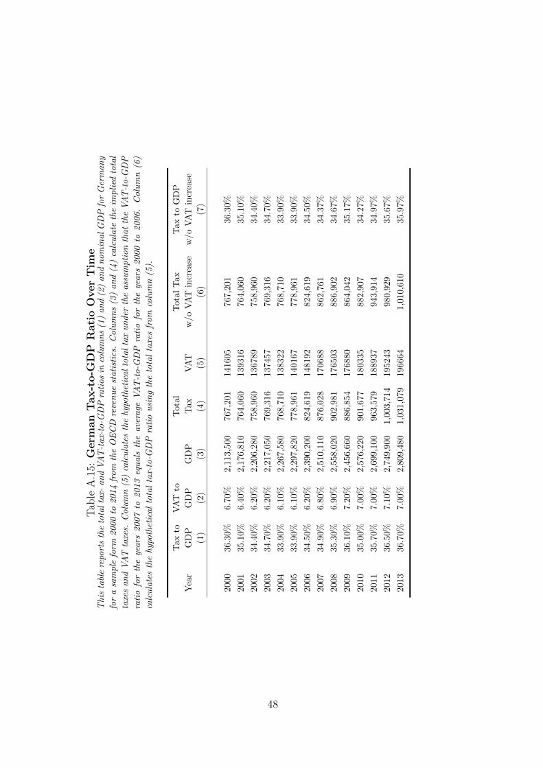
Tab

leA

.15:

Germ

an

Tax-t

o-G

DP

Rati

oO

ver

Tim

eT

his

tabl

ere

port

sth

eto

tal

tax-

an

dV

AT

-tax-

to-G

DP

rati

os

inco

lum

ns

(1)

an

d(2

)an

dn

om

inal

GD

Pfo

rG

erm

an

y

for

asa

mple

form

2000

to2014

from

the

OE

CD

reve

nu

est

ati

stic

s.C

olu

mn

s(3

)an

d(4

)ca

lcu

late

the

impli

edto

tal

taxe

san

dV

AT

taxe

s.C

olu

mn

(5)

calc

ula

tes

the

hyp

oth

etic

al

tota

lta

xu

nder

the

ass

um

pti

on

that

the

VA

T-t

o-G

DP

rati

ofo

rth

eye

ars

2007

to2013

equ

als

the

ave

rage

VA

T-t

o-G

DP

rati

ofo

rth

eye

ars

2000

to2006

.C

olu

mn

(6)

calc

ula

tes

the

hyp

oth

etic

al

tota

lta

x-to

-GD

Pra

tio

usi

ng

the

tota

lta

xes

from

colu

mn

(5).

Tax

toV

AT

toT

ota

lT

ota

lT

ax

Tax

toG

DP

Yea

rG

DP

GD

PG

DP

Tax

VA

Tw

/o

VA

Tin

crea

sew

/o

VA

Tin

crea

se

(1)

(2)

(3)

(4)

(5)

(6)

(7)

2000

36.3

0%6.

70%

2,113,5

00

767,2

01

141605

767,2

01

36.3

0%

2001

35.1

0%6.

40%

2,176,8

10

764,0

60

139316

764,0

60

35.1

0%

2002

34.4

0%6.

20%

2,206,2

80

758,9

60

136789

758,9

60

34.4

0%

2003

34.7

0%6.

20%

2,217,0

50

769,3

16

137457

769,3

16

34.7

0%

2004

33.9

0%6.

10%

2,267,5

80

768,7

10

138322

768,7

10

33.9

0%

2005

33.9

0%6.

10%

2,297,8

20

778,9

61

140167

778,9

61

33.9

0%

2006

34.5

0%6.

20%

2,390,2

00

824,6

19

148192

824,6

19

34.5

0%

2007

34.9

0%6.

80%

2,510,1

10

876,0

28

170688

862,7

61

34.3

7%

2008

35.3

0%6.

90%

2,558,0

20

902,9

81

176503

886,9

02

34.6

7%

2009

36.1

0%7.

20%

2,456,6

60

886,8

54

176880

864,0

42

35.1

7%

2010

35.0

0%7.

00%

2,576,2

20

901,6

77

180335

882,9

07

34.2

7%

2011

35.7

0%7.

00%

2,699,1

00

963,5

79

188937

943,9

14

34.9

7%

2012

36.5

0%7.

10%

2,749,9

00

1,0

03,7

14

195243

980,9

29

35.6

7%

2013

36.7

0%7.

00%

2,809,4

80

1,0

31,0

79

196664

1,0

10,6

10

35.9

7%

48