NBER WORKING PAPER SERIES

INFLATION, MONETARY POLICY AND STOCK MARKET CONDITIONS

Michael D. BordoMichael J. Dueker

David C. Wheelock

Working Paper 14019http://www.nber.org/papers/w14019

NATIONAL BUREAU OF ECONOMIC RESEARCH1050 Massachusetts Avenue

Cambridge, MA 02138May 2008

The authors thank Christopher Martinek for research assistance. The views expressed in this paperare not necessarily official positions of the Federal Reserve Bank of St. Louis, the Federal ReserveSystem, Russell Investments, or the views of the National Bureau of Economic Research.

NBER working papers are circulated for discussion and comment purposes. They have not been peer-reviewed or been subject to the review by the NBER Board of Directors that accompanies officialNBER publications.

© 2008 by Michael D. Bordo, Michael J. Dueker, and David C. Wheelock. All rights reserved. Shortsections of text, not to exceed two paragraphs, may be quoted without explicit permission providedthat full credit, including © notice, is given to the source.

Inflation, Monetary Policy and Stock Market ConditionsMichael D. Bordo, Michael J. Dueker, and David C. WheelockNBER Working Paper No. 14019May 2008JEL No. E31,E52,G12,N12,N22

ABSTRACT

This paper examines the association between inflation, monetary policy and U.S. stock market conditionsduring the second half of the 20th century. We estimate a latent variable VAR to examine how macroeconomicand policy shocks affect the condition of the stock market. Further, we examine the contribution ofvarious shocks to market conditions during particular episodes and find evidence that inflation andinterest rate shocks had particularly strong impacts on market conditions in the postwar era. Disinflationshocks promoted market booms and inflation shocks contributed to busts. We conclude that centralbanks can contribute to financial market stability by minimizing unanticipated changes in inflation.

Michael D. BordoDepartment of EconomicsRutgers UniversityNew Jersey Hall75 Hamilton StreetNew Brunswick, NJ 08901and NBERbordo@econ.rutgers.edu

Michael J. DuekerRussell Investments909 A StreetTacoma, WA 98402MDueker@Russell.com

David C. WheelockResearch DivisionFederal Reserve Bank of St. LouisP.O. Box 442St. Louis, MO 63166-0442david.c.wheelock@stls.frb.org

1

I. Introduction

The association between monetary policy and the performance of stock and other

asset markets has long piqued the interest of economists and policymakers. Stocks are

claims on real assets and, hence, monetary neutrality implies that monetary policy should

not affect real stock prices in the long run. Although real stock returns and inflation have

been negatively correlated historically (Fama and Schwert, 1977), the correlation is

widely seen as an anomaly resulting from the simultaneous impacts of real economic

activity on inflation and stock returns (Fama, 1981).1

Despite the presumed irrelevance of inflation for real stock returns in the long run,

researchers have found considerable evidence that monetary policy can affect real stock

prices in the short run.2 Further, economists have conjectured that the nature of the

monetary policy regime can affect the performance of asset markets over longer horizons.

Goodfriend (2003), for example, argues that before 1980 the policies of the Federal

Reserve and other central banks were an important source of macroeconomic and

financial instability that could explain the negative correlation between real stock prices

and inflation. Rising inflation, for example, tended to depress stock returns because

higher expected inflation would increase long-term interest rates (and thereby raise the

rate at which investors discount future dividends) and because monetary policy actions to

limit inflation would tend to slow economic activity (and thereby depress current and

forecast earnings).3

1 See also Lee (1992) or Rapach (2001; 2002). By contrast, Modigliani and Cohn (1979) argue that the negative correlation between stock returns and inflation reflects “inflation illusion” on the part of investors. For supporting evidence, see Campbell and Vuolteenaho (2004) and Ritter and Warr (2002). 2 See Bernanke and Kuttner (2005) and He (2006), and references therein for estimates of the short-run impact of monetary policy on stock prices. 3 Some economists argue that asset price bubbles or other forms of financial instability are more likely when monetary policy fails to maintain a stable price level (e.g., Schwartz, 1995; Woodford, 2003).

2

The “Fed model” of stock returns, which links market returns to inflation through

nominal bond yields has had considerable success as a historical description of stock

prices (Campbell and Vuolteenaho, 2004), and many observers believe that disinflation

contributed to the U.S. stock market boom of the 1990s, as well as to booms historically.4

Indeed, at a Federal Open Market Committee meeting in 1996, Chairman Alan

Greenspan observed:

We have very great difficulty in monetary policy when we confront stock market bubbles. That is because, to the extent that we are successful in keeping product price inflation down, history tells us that price-earnings ratios under those conditions go through the roof. What is really needed to keep stock market bubbles from occurring is a lot of product price inflation, which historically has tended to undercut stock markets almost everywhere. There is a clear tradeoff. If monetary policy succeeds in one, it fails in the other. (FOMC meeting transcript, September 24, 1996, pp. 30-31)5

Thus, while monetary policy and inflation probably have little or no long-run impact on

real stock returns, the view that monetary policy can affect the stock market in the short-

to-intermediate run both through unanticipated policy shocks and through its impact on

inflation is widely held.

In this paper we seek to quantify the extent to which various macroeconomic and

policy shocks, including inflation shocks, can explain the behavior of U.S. real stock

prices during the second half of the 20th century. Prior research has found that the impact

of monetary policy actions on stock returns has varied over time with changes in market

conditions. Chen (2007), for example, uses a Markov-switching model to identify bull

and bear markets, and finds that monetary policy shocks have a larger impact on market

4 Bordo and Wheelock (2007) review the histories of major 20th century stock market booms in the United States and nine other countries and find that booms usually arose when inflation was below its long-run average, and that booms typically ended when inflation began to rise and/or monetary authorities tightened policy in response to rising or a threatened rise in inflation. 5 Borio and Lowe (2002) argue similarly, contending that disinflation can promote financial imbalances, including stock market bubbles.

3

returns in bear markets and that contractionary monetary policy increases the probability

of the market moving to a bear market state.

We also investigate the impact of macroeconomic and policy shocks on stock

market conditions, and whether the response of real stock prices to shocks differs during

extended periods of unusually rapid growth and decline in real stock prices (“booms” and

“busts”) compared with periods of more normal market conditions. Unlike Chen (2007),

who assumes that the stock market is always in either a bull- or a bear-market state, our

approach allows a majority of observations to belong to a middle (“normal”) category,

which enables us to test explicitly for differences in behavior during highly unusual

episodes. If all observations were forced to lie within either a boom or bust state, the

magnitude of the difference between these two qualitative states would be diluted if most

observations actually belong to a middle (“normal”) category. The historical record

suggests that equity and other asset markets are characterized by occasional extended

periods of extreme optimism and extreme pessimism that seem to defy fundamentals.6 If

true, it would suggest that the impact of a given policy or economic shock on real stock

prices might differ during such periods from more normal times.

We employ a latent-variable vector autoregression (Qual-VAR) model to estimate

the impact of macroeconomic and policy shocks on the growth of real stock prices and

stock market conditions. By explicitly taking account of market conditions, the Qual-

VAR is well suited to studying experiences that fall outside the norm, such as stock

market booms and busts, that comprise relatively little of the overall sample variance of

stock price movements. Thus, the Qual-VAR provides evidence about whether

6 Discussions of this phenomenon include Kindleberger (1989) and Shiller (2005).

4

relationships observed during booms or busts differ from those of periods that could be

characterized as normal.

Qual-VAR models have been used to examine recessions, where researchers are

interested in estimating relationships during periods of unusually weak activity that

nonetheless account for relatively little of the overall sample variance of output (e.g.,

Dueker, 2005; Dueker and Nelson, 2006). However, unlike recession dates, which a

researcher can reasonably treat as data, the identification of when the stock market is in a

boom or bust state inherently involves judgment on the part of the researcher, which is a

potential drawback of the basic Qual-VAR approach.7 To address this drawback, we use

a hybrid approach that combines an otherwise standard Qual-VAR model with a dynamic

factor model. This hybrid model allows the data to partly identify market conditions

guided by our initial classification of periods of exceptionally rapid and prolonged

increase in real stock prices as “booms,” and significant decline as “busts.”

From the Qual-VAR estimation we find evidence that inflation shocks have had a

significant impact on the U.S. stock market historically, with disinflation shocks

promoting booms and inflation shocks promoting busts. Interest rate shocks also have

had a large impact, with unexpected increases in the long-term interest rate pushing the

market toward a bust and unexpected rate declines moving the market toward a boom.

Further, our counterfactual analysis indicates that disinflation shocks can explain more of

the stock market boom of 1995-99 than output shocks, and that inflation shocks also

contributed to prior episodes of market instability. Our results are thus consistent with

7 See Harding and Pagan (2006) for warnings about working with constructed classifications. This problem arises in many contexts, e.g., in studies of financial or currency crises (e.g., Kaminsky and Reinhart, 1999).

5

the view that a policy regime that minimizes unanticipated fluctuations in inflation can

contribute to financial market stability.

Section II describes our econometric model and approach for identifying market

conditions. Section III presents estimation results and a counterfactual exercise to

identify the importance of various shocks on market conditions throughout the period

spanned by our data. Section IV concludes.

II. Estimating the Impact of Macroeconomic and Policy Shocks on Real Stock

Prices

Several studies have investigated the impact of macroeconomic shocks on stock

market variables using vector autoregression techniques.8 However, unlike prior studies,

we focus on the extent to which macroeconomic and policy shocks can explain changes

in stock market conditions, and whether the impact of shocks on real stock prices

historically has varied with the market’s condition. Relatively little of the overall sample

variance of stock returns occurs during booms or busts because those episodes occur

infrequently. Hence, estimates from models that do not account for the condition of the

market will be heavily influenced by data from normal periods. Our latent variable

vector autoregression (Qual-VAR) approach can provide evidence about whether the

relationships we observe during booms and busts differ from those of more ordinary

market conditions.

A potential drawback of the basic Qual-VAR approach to modeling stock market

conditions stems from its reliance on the subjective determination by the researcher of

when the market is in a boom or bust state. In making use of a constructed chronology of

financial booms and busts, one has to decide how heavily to rely on the judgmental dates. 8 Recent examples include Lee (1992), Rapach (2001), and Hayford and Malliaris (2004).

6

If they are given full credence, a multivariate dynamic ordered probit approach, such as

the Qual-VAR from Dueker (2005) and Dueker and Nelson (2006), would treat the

constructed chronology as part of the data. However, in the absence of widely accepted

criteria for identifying differences in market conditions, we adopt the hybrid approach

described below that makes the determination of market conditions at least partly

endogenous, and thereby lessens the influence of our own judgments about how to define

booms and busts. This approach could be applied in other settings where the

identification of an episode being studied is based on ad hoc criteria.

Econometric Model

To fix ideas, consider a generic unobserved component state-space model with the

following state equation, where X are the observable variables and z is the latent

unobserved component:

1

1

1 2

,

,

00

0 1 00

0

t tX

zX zzt z t

t t

t

z t

X

XX XzX Xcz c zz z

ε

ε

−

−

− −

Φ Φ⎛ ⎞ ⎛⎛ ⎞ ⎛ ⎞⎜ ⎟ ⎜⎜ ⎟ ⎜ ⎟= + Φ Φ⎜ ⎟ ⎜⎜ ⎟ ⎜ ⎟

⎜ ⎟⎜ ⎟⎜ ⎟ ⎜⎝ ⎠⎝ ⎠⎝ ⎠ ⎝⎛ ⎞⎜ ⎟

+ ⎜ ⎟⎜ ⎟⎜ ⎟⎝ ⎠

⎞⎟⎟⎟⎠

t

(1)

The measurement equation is

( )1

0 0t

t

t

XX I z

z −

⎛ ⎞⎜= ⎜⎜ ⎟⎝ ⎠

⎟⎟ (2)

As an example of the Qual-VAR approach, consider the following relationship

between the latent variable and the three categories of stock market conditions:

7

1

1 2

2

t

t

t

bust state iff z cnormal state iff c z c

boom state iff z c

<≤ <>

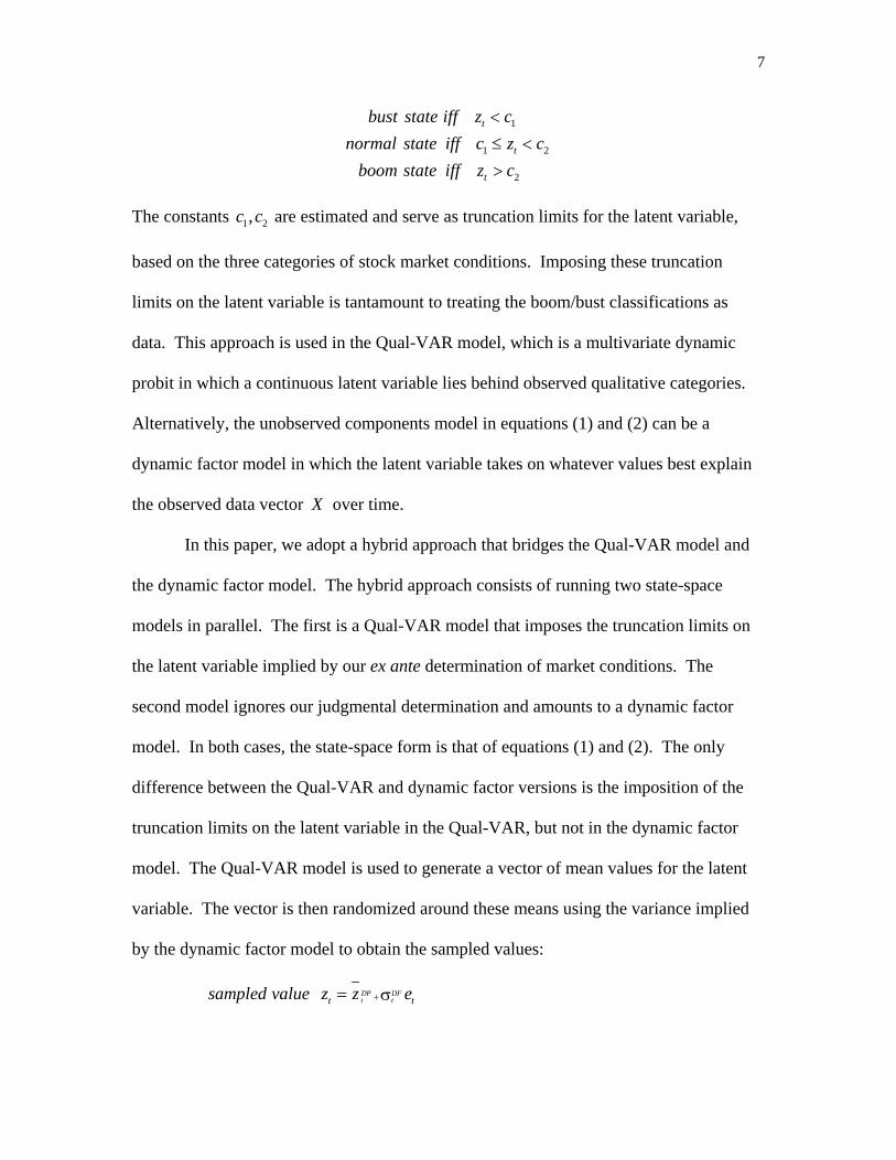
The constants are estimated and serve as truncation limits for the latent variable,

based on the three categories of stock market conditions. Imposing these truncation

limits on the latent variable is tantamount to treating the boom/bust classifications as

data. This approach is used in the Qual-VAR model, which is a multivariate dynamic

probit in which a continuous latent variable lies behind observed qualitative categories.

Alternatively, the unobserved components model in equations (1) and (2) can be a

dynamic factor model in which the latent variable takes on whatever values best explain

the observed data vector

1 2,c c

X over time.

In this paper, we adopt a hybrid approach that bridges the Qual-VAR model and

the dynamic factor model. The hybrid approach consists of running two state-space

models in parallel. The first is a Qual-VAR model that imposes the truncation limits on

the latent variable implied by our ex ante determination of market conditions. The

second model ignores our judgmental determination and amounts to a dynamic factor

model. In both cases, the state-space form is that of equations (1) and (2). The only

difference between the Qual-VAR and dynamic factor versions is the imposition of the

truncation limits on the latent variable in the Qual-VAR, but not in the dynamic factor

model. The Qual-VAR model is used to generate a vector of mean values for the latent

variable. The vector is then randomized around these means using the variance implied

by the dynamic factor model to obtain the sampled values:

DP DFt tt tsampled value z z e+ = σ

8

where DP denotes a value implied by the Qual-VAR (dynamic probit) model, DF refers

to the dynamic factor model and e is a standard normal shock. Note that the sampled

values of the latent variable need not conform with the truncation limits imposed in the

Qual-VAR. Also note that, in keeping with the Bayesian nature of the estimation

procedure outlined here, one can easily scale the variances up or down. A scaling factor

less than one implies a greater degree of confidence in the ex ante determination of

market conditions, which amounts to a stronger prior on their relevance. Similarly, a

scaling factor greater than one amounts to a weaker prior on the ex ante determination.

We set the scaling factor to 1.0, which we consider to be a neutral baseline value, to

generate the results presented here.

A key property of the hybrid procedure is that the draws of the latent variable can

lie outside the truncation limits and so the model-implied category for a given

observation can differ from the category assigned to it by the researcher. Nevertheless,

unlike the dynamic factor model, by centering the randomization of the latent variable at

the values implied by the ex ante determination, the latent variable is tailored to reflect

the judgmental determination on average across the sample period. In this way, the

hybrid Qual-VAR / dynamic factor model helps overcome the “what does the factor

represent?” question that hinders interpretation of dynamic factor models. At the same

time, however, the hybrid model also addresses concerns about the accuracy with which

the researcher assigned observations to particular categories.

We estimate our hybrid model using a Bayesian Markov Chain Monte Carlo

estimation procedure in which the randomized values of the latent variable are treated as

a proposal value in a Metropolis-Hastings step. This proposal draw is either accepted or

9

rejected depending on how the draw fits the data density.9 The proposal density has the

mean implied by the Qual-VAR and the variance implied by the dynamic factor model.

The data density is derived from the forecast errors for the observed data X conditional

on a vector of values for the latent variable . According to the Metropolis-Hastings

sampling algorithm for the latent variable, the proposal value is accepted with probability

z

( ) ( ) ( )( ) ( )

min ,1old new

Tnewnew old

T

g z f X zz

g z f X zα

⎧ ⎫⎪ ⎪= ⎨ ⎬⎪ ⎪⎩ ⎭

The current value is retained if the proposal value is rejected by a uniform draw on

the unit interval, where the acceptance probability is α, is the proposal density for the

latent variable vector and

oldz

g

f is the target density for the data conditional on a set of values

for the latent variable.

Probit models are nonlinear regressions. Even though we are working in a vector

autoregression framework, the latent variable leads to a nonlinear response of the

macroeconomic variables to a change in stock prices. If a change in stock prices is

associated with a change in market conditions, say from normal to boom, then the effect

is magnified (or possibly dampened) relative to a change in stock prices of the same size

that is not associated with a change in conditions. This nonlinearity arises because the

latent variable is relatively constant within each category of market conditions but

undergoes sizable jumps between categories.

Data and Model Specification

We use the hybrid Qual-VAR / dynamic factor model to estimate the effects of

output, inflation, and other shocks on real stock prices and the latent variable representing

9 See Chib and Greenberg (1995) for details about the estimation procedure.

10

market conditions. First, we identify extended periods of exceptional increase or decline

in real stock prices (the nominal S&P 500 index deflated by the Consumer Price Index)

using the approach of Pagan and Sossounov (2003). Specifically, we identify peaks and

troughs in the real stock price within rolling, 25-month windows. To ensure that peaks

and troughs alternate, we eliminate all but the highest maximum that occurred before a

subsequent trough and all but the lowest minimum that occurred before a subsequent

peak. We classify as booms all periods of at least 36 months from trough to peak with an

average annual rate of increase in the real stock price index of at least 10 percent or of at

least 24 months with an annual rate of increase of at least 20 percent. We define market

busts as all periods of at least 12 months from a market peak to a market trough in which

the index declined at an average rate of at least 20 percent per year. Following Pagan and

Sossounov (2003), we also treat the 1987 stock market crash as a bust even though the

stock market decline lasted for less than 12 months. Similarly, we also treat the 10-

month decline in 1966 as a bust. Table 1 lists the boom and bust periods we identify and

the average annual percentage change in the stock market index during each episode. For

comparison, the real stock price index rose at an average annual rate of 4.4 percent

throughout 1947-2004.

As described above, our estimation procedure uses the boom and bust periods

listed in Table 1 as starting values, but the implied classifications for individual periods

are determined endogenously by fitting the model to the data, thereby reducing the extent

to which our estimation results are driven by our personal judgments about how to define

booms and busts. Our ex ante determination of market conditions guides the sampling of

the latent variable but some percentage of the Markov Chain Monte Carlo draws for a

11

given observation will imply a different classification than the one we chose. For

example, not all draws will have zt > c2 within periods listed as booms in Table 1.

Figures 1-3 show the percentage of Qual-VAR draws in which the given model-implied

stock market category corresponds with the market booms and busts listed in Table 1.

For example, Figure 1 shows the percentage of draws for which zt > c2 within periods

designated ex ante as booms (indicated by the shaded regions). For the most part, the

figures show that a high percentage of the model-implied draws of the latent variable lie

within the categories we identified ex ante. Note, however, that the percentages are by no

means constant during these periods, illustrating the difference between the latent market

conditions variable and the ex ante determination of market booms and busts.

III. Estimation Results

The hybrid Qual-VAR / dynamic factor model allows us to present results through

familiar vector autoregression tools such as impulse responses and variance

decompositions. These tools are available once we specify an ordering of the VAR

variables. The selected ordering also permits us to conduct counterfactual analysis by

way of shutting down one structural shock at a time and then calculating counterfactual

histories of the model variables. In doing so, we can investigate the extent to which stock

market conditions would have differed over our sample period in the absence of various

shocks.

We are interested in estimating the impact of shocks to output, inflation, and

various other nominal variables on real stock prices and market conditions. To apply

standard VAR tools to our hybrid model, we identify shocks through the following

ordering of variables: (log) industrial production, inflation, money stock growth, 10-year

12

Treasury security yield, 3-month Treasury bill yield, real stock price index, and the latent

stock market variable (z), representing market conditions.10 The variables are ordered so

that variables that are pre-determined to a greater extent appear first. Shock measures for

variables ordered last condition on a greater number of forecast errors and therefore

ought to be cleaner. In ordering the stock market variables last, we assume that stock

market shocks have no contemporaneous impact on the other variables in the model,

which seems preferable to assuming that policy and other shocks have no

contemporaneous impact on the stock market.11 We use monthly data for August 1952 –

December 2005, and six lags in the Qual-VAR autoregressions.

Figure 4 presents impulse responses of the real stock price index (S&P 500) and

stock market conditions for output (industrial production) and inflation shocks. The

figures show point estimates and the bounds of two standard deviations on either side of

the point estimates. The initial impacts of output shocks on the real stock price index and

on market conditions are both positive, but die out quickly and are not statistically

significant. By contrast, inflation shocks have a negative, statistically significant and

persistent impact on both the real stock price and market conditions. Not only do positive

inflation shocks reduce the real stock price, they also move market conditions away from

boom and normal states toward busts. Moreover, the impact on stock market conditions

10 We experimented by excluding money stock growth and by reversing the order of the 10-year and 3-month Treasury security yields. In so doing we obtained results that are qualitatively similar to those reported here except as noted below. See the appendix for variable definitions and data sources. 11 Evidence on whether or not the Fed reacted to the stock market boom of the 1990s has been mixed. Rigobon and Sack (2003) use an identification scheme based on the heteroskedasticity of stock returns to sort out the simultaneous response of equity prices and interest rates. They estimate that during 1985-99, a 5 percent rise in the S&P 500 stock price index increased the likelihood of a 25 basis point policy tightening by about one half. Cecchetti (2003) also concludes that the Fed tightened in response to the booming stock market in the 1990s. On the other hand, Hayford and Malliaris (2004) estimate a forward-looking Taylor Rule and find no evidence that the Fed reacted to the stock market during the 1990s, and Meyer (2004) contends that the Fed did not react systematically to movements in the stock market during his tenure as a member of the Federal Reserve Board of Governors, 1996-2002.

13

appears to induce further decline in real stock prices. In a simple VAR model that does

not include the latent stock market conditions variable, inflation shocks account for only

25 percent of the variance of the real stock price at a 36 month horizon – a horizon at

which the central bank is certainly responsible for the thrust of inflation shocks.

However, in the hybrid Qual-VAR model, which allows both a direct effect of inflation

on stock prices and an indirect effect via stock market conditions, inflation shocks

account for almost 33 percent of the variance of real stock prices. Thus, our latent

variable approach captures a quantitatively important channel by which inflation shocks

affect real stock prices through their impact on stock market conditions.

Figure 5 shows the impacts of shocks to money stock growth and interest rates on

the stock market index and market conditions. Money stock growth shocks do not have a

statistically significant impact on the market. However, shocks to the long-term interest

rate have a negative, statistically-significant and persistent impact on the real stock price.

The estimated impact on market conditions is also negative, though statistically

significant only for the first three months. Rising interest rates can depress stock prices

by raising the rate at which investors discount future earnings and/or by reducing the

growth rate of earnings, and thus it is not surprising to find that interest rate shocks tend

to reduce stock prices and push the market away from boom conditions. Finally,

controlling for shocks to the long-rate, we find that the initial impact of short-term

interest rate shocks on the real stock price is negative (though not statistically significant)

whereas the initial impact on stock market conditions is positive. Over the long-run,

14

however, short-term interest rate shocks have a negative impact on both the real stock

price and stock market conditions.12

Next we examine the impacts of output, inflation, and interest rate shocks on

stock market conditions over time by comparing counterfactual values of the latent

market conditions variable constructed by shutting down individual shocks with values

estimated from the full model. The black lines in Figures 6-8 show the posterior mean

values of the latent stock market conditions variable zt relative to the constants c1 and c2

that demarcate the bust, normal, and boom regions (c1 and c2 are indicated by the dashed

horizontal lines).13 The grey lines in Figures 6-8 show counterfactual values of the latent

variable calculated by setting the indicated structural shock to zero. This provides an

indication of the importance of various shocks to stock market conditions throughout our

sample period.

Figure 6 shows that output shocks can account for little of the change in stock

market conditions over time, as the simulated path of market conditions is nearly

identical to the actual path of the latent variable. Inflation shocks appear to have had a

more pronounced impact on the market. Figure 7 indicates, for example, that stock

market conditions would have been stronger in the early 1990s but weaker later in the

decade in the absence of inflation shocks. U.S. inflation spiked following a sharp

increase in energy prices at the start of the Gulf War in 1990. Although inflation then

fell, it remained above historical norms and higher than one might forecast given the 12 We find the impact of short-term interest rate shocks to be somewhat sensitive to whether the short-term interest rate is ordered before or after the long-term interest rate in the Qual-VAR as well as to the estimation period. Short-term interest rate shocks are found to have a stronger negative impact on stock prices if the short-term rate is placed before the long-term rate in the variable ordering, and also when the estimation is restricted to the post-1980 period. It should be noted, of course, that shocks to short-term interest rates capture idiosyncratic movements and not the endogenous response of interest rates or monetary policy to inflation, output or stock prices. 13 The values shown for c1 and c2 are posterior means estimated under the restriction that c1 < 0 and c2 > 0.

15

stance of monetary policy.14 Our counterfactual series indicates that positive inflation

shocks kept a lid on the stock market before 1995. Further decline in the inflation rate in

the mid-1990s, however, appears to have promoted a boom state during 1995-99

according to our counterfactual. In the absence of unexpected decline in inflation, the

counterfactual suggests the stock market would have dropped out of a boom state in mid-

1997 into the normal region.

Inflation shocks were also important for U.S. stock market conditions at other

times over our sample period. For example, our counterfactual indicates that lower-than-

expected inflation can help explain the stock market boom of 1953-56, whereas higher-

than-expected inflation may have contributed to the market bust of 1973-75. Further, we

find that stock market conditions would have been decidedly weaker in the absence of

shocks associated with disinflation in the early 1980s.

Figure 8 presents a counterfactual path for market conditions in the absence of

shocks to the long-term Treasury security yield. The counterfactual series indicates, for

example, that market conditions might have been stronger in the absence of positive

interest rate shocks during 1978-81, especially after the abrupt tightening of monetary

policy in October 1979. However, negative interest rate shocks can help account for the

stock market boom conditions of the mid-1980s and late 1990s. Thus, our results

indicate that unanticipated changes in inflation and interest rates were important

determinants of both real stock prices and market booms and busts over the post-war era.

14 In an op-ed article in the Wall Street Journal on 23 October 1992, Milton Friedman argued that “monetary policy has been extremely tight, not easy, in the U.S.” Noting that M2 growth had fallen below 2 percent during the prior four quarters, Friedman argued that “continuation of M2 growth at 2% per year would imply actual deflation, not negligible inflation.” In the event, inflation remained between 2.5 and 3 percent until 1997.

16

IV. Conclusion

Policymakers and others often link the performance of the stock market to

changes in inflation and monetary policy, especially during extended periods of rapid

appreciation or decline in real stock prices. This paper presents an empirical model that

allows the impact of macroeconomic and policy shocks on real stock prices to vary with

stock market conditions. Further, the approach enables us to examine the contribution of

various shocks to stock market conditions during particular episodes. Thus, the use of a

latent boom/bust measure of stock market conditions captures an additional channel

through which a central bank’s efforts to reduce fluctuations in inflation can contribute to

greater asset market stability. Methodologically, our hybrid Qual-VAR / dynamic factor

model offers an innovative approach to estimating the determinants of asset booms and

busts that lessens the influence of researcher judgment on the identification of market

conditions.

The evidence reported here provides support for the view that unanticipated

changes in inflation and interest rates have played important roles in major movements in

the U.S. stock market since World War II. We find that inflation and interest rate shocks

have large, negative impacts on stock market conditions, apart from their effects on real

stock prices. Disinflationary shocks, for example, can help explain the U.S. stock market

boom of 1994-2000, whereas inflationary shocks can help explain the bust of 1973-74.

The policy lesson we draw concerns not necessarily what policymakers ought to do when

faced with a bubbling stock market but how they can contribute to equity market stability

by minimizing unanticipated fluctuations in inflation. Similarly, the impulse responses to

long-term interest rate shocks suggest that monetary policies that induce financial

17

markets to reduce inflation risk premia in long-term interest rates will promote financial

market stability.

18

References

Bernanke, Ben S. and Kuttner, Kenneth N. “What Explains the Stock Market’s Reaction to Federal Reserve Policy?” Journal of Finance 60(3), June 2005, pp. 1221-57.

Bordo, Michael and Wheelock, David C. “Stock Market Booms and Monetary Policy in the 20th Century.” Federal Reserve Bank of St. Louis Review 89 (2), March/April 2007, pp. 91-122.

Borio, Claudio and Lowe, Philip. “Asset Prices, Financial and Monetary Stability: Exploring the Nexus.” Working paper no. 114, Bank for International Settlements, July 2002.

Campbell, John Y. and Vuolteenaho, Tuomo. “Inflation Illusion and Stock Prices.” American Economic Review Papers and Proceedings 94 (2), May 2004, pp. 19-23.

Cecchetti, Stephen G. “What the FOMC Says and Does When the Stock Market Booms.” Prepared for the Reserve Bank of Canada conference on Asset Prices and Monetary Policy. Sydney, Australia, August 2003.

Chen, Shiu-Sheng. “Does Monetary Policy Have Asymmetric Effects on Stock Returns?” Journal of Money, Credit and Banking 39 (2-3), March-April 2007, pp. 667-88.

Chib, Siddhartha and Greenberg, Edward. “Understanding the Metropolis-Hastings Algorithm.” American Statistician 49, 1995, pp. 327-35.

Dueker, Michael J. “Dynamic Forecasts of Qualitative Variables: A Qual VAR Model of U.S. Recessions.” Journal of Business and Economic Statistics 23 (1), January 2005, pp. 96-104.

Dueker, Michael J. and Nelson, Charles R. “Business Cycle Filtering of Macroeconomic Data Via a Latent Business Cycle Index.” Macroeconomic Dynamics 10 (5), November 2006, pp. 573-94.

Fama, Eugene F. “Stock Returns, Real Activity, Inflation, and Money.” American Economic Review 71 (4), September 1981, pp. 545-65.

Fama, Eugene F. and Schwert, G. William. “Asset Returns and Inflation,” Journal of Financial Economics 5, 1977, pp. 115-46.

Friedman, Milton. “Too Tight for a Strong Economy,” The Wall Street Journal, 23 October 1992, p. A12.

Goodfriend, Marvin. “Interest Rates Policy Should Not React Directly to Asset Prices,” in William C. Hunter, George G. Kaufman, and Michael Pomerleano, eds., Asset

19

Price Bubbles: The Implications for Monetary, Regulatory, and International Policies. Cambridge, MA: The MIT Press, 2003, pp. 445-57.

Harding, Don and Adrian Pagan. “The Econometric Analysis of Constructed Binary Time Series.” Working Paper #963, University of Melbourne, 2006.

Hayford, Marc D. and Malliaris, A.G.. “Monetary Policy and the U.S. Stock Market. Economic Inquiry, July 2004, 42(3), pp. 387-401.

He, Ling T. “Variations in Effects of Monetary Policy on Stock Market Returns in the Past Four Decades.” Review of Financial Economics 15, 2006, pp. 331-49.

Kaminsky, Graciela L. and Reinhart, Carmen M. “The Twin Crises: The Causes of Banking and Balance-of-Payments Problems.” American Economic Review 89 (3), June 1999, pp. 473-500.

Kindleberger, Charles P. Manias, Panics and Crashes: A History of Financial Crises. Second Edition. London: Macmillan, 1989.

Lee, Bong-Soo. “Causal Relations Among Stock Returns, Interest Rates, Real Activity, and Inflation.” Journal of Finance 47 (4), September 1992, pp. 1591-1603.

Meyer, Laurence H. A Term at the Fed: An Insider’s View. New York: Harper Business, 2004.

Modigliani, Franco, and Cohn, Richard. “Inflation, Rational Valuation, and the Market.” Financial Analysts Journal 37 (3), March/April 1979, pp. 24-44.

Pagan, Adrian R. and Sossounov, Kirill A. “A Simple Framework for Analysing Bull and Bear Markets.” Journal of Applied Econometrics, January/February 2003, 18(1), pp. 23-46.

Rapach, David E. “The Long-Run Relationship Between Inflation and Real Stock Prices.” Journal of Macroeconomics 24, 2002, pp. 331-51.

Rapach, David E. “Macro Shocks and Real Stock Prices.” Journal of Economics and Business 53, 2001, pp. 5-26.

Rigobon, R. and Sack, Brian. “Measuring the Reaction of Monetary Policy to the Stock Market.” Quarterly Journal of Economics, May 2003, 118(2), pp. 639-69.

Ritter, Jay R. and Warr, Richard S. “The Decline of Inflation and the Bull Market of 1982-1999.” Journal of Financial and Quantitative Analysis 37 (1), March 2002, pp. 29-61.

Schwartz, Anna J. “Why Financial Stability Depends on Price Stability.” Economic Affairs 15(4), Autumn 1995, pp. 21-25.

20

Shiller, Robert J. Irrational Exuberance. Second Edition. Princeton: Princeton University Press, 2005.

Woodford, Michael. Interest and Prices: Foundations of a Theory of Monetary Policy. Princeton: Princeton University Press, 2003.

21

Appendix This appendix provides information about the data and sources used in this paper. Stock Price Index: Standard and Poor's 500 Composite Index, monthly average of daily data. Source: Haver Analytics. Consumer Price Level: All Items Consumer Price Index for urban consumers (not seasonally adjusted, 1982-84=100). Source: Haver Analytics. Output: Index of Industrial Production (seasonally adjusted, 2002=100). Source: Haver Analytics. Money Stock: Broad money stock (1952-58). Source: Friedman and Schwartz (1963), Table A-1, column 8. Board of Governors M2 (1959-2005). Source: Federal Reserve Bank of St. Louis. Long-term Treasury Yield: Yield on 10-year constant maturity Treasury security. Source: Haver Analytics. Short-term Interest Rate: Secondary market (discount) yield on 3-month Treasury bills (1953-2005). Source: Haver Analytics.

Boom Start Boom EndAvg. Annual

% Change Bust Start Bust EndAvg. Annual

% ChangeSept. 1953 Apr. 1956 28.8 Dec. 1961 June 1962 -49.8June 1962 Jan. 1966 13.3 Jan. 1966 Oct. 1966 -29.2July 1984 Aug. 1987 22.9 Dec. 1968 July 1970 -26.5Apr. 1994 Aug. 2000 17.1 Jan. 1973 Dec. 1974 -38.3

Nov. 1980 July 1982 -19.9Aug. 1987 Dec. 1987 -91.0Aug. 2000 Feb. 2003 -23.7

Source: Text.

Table 1U.S. Stock Market Booms and Busts

Booms Busts

Figure 1: United States Boom Category Model-Implied Draws of the Latent Variable

0

0.2

0.4

0.6

0.8

1

1952 1956 1960 1964 1968 1972 1976 1980 1984 1988 1992 1996 2000 2004

Boom Periods Model-implied Draws of the Latent Variable

Figure 2: United States Bust Category Model-Implied Draws of the Latent Variable

0

0.2

0.4

0.6

0.8

1

1952 1956 1960 1964 1968 1972 1976 1980 1984 1988 1992 1996 2000 2004

Bust Periods Model-implied Draws of the Latent Variable

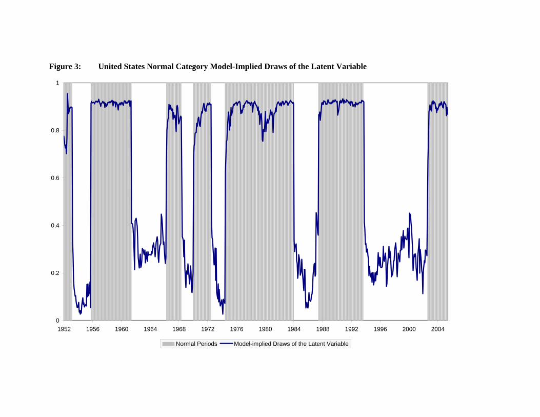
Figure 3: United States Normal Category Model-Implied Draws of the Latent Variable

0

0.2

0.4

0.6

0.8

1

1952 1956 1960 1964 1968 1972 1976 1980 1984 1988 1992 1996 2000 2004

Normal Periods Model-implied Draws of the Latent Variable

Figure 4: Impulse Response Functions of Stock Market Variables to Output and Inflation Shocks

-.025

-.020

-.015

-.010

-.005

.000

.005

.010

5 10 15 20 25 30 35

Response of Real S&P 500to Output Shock

-.12

-.08

-.04

.00

.04

.08

5 10 15 20 25 30 35

Response of Stock Market Conditionsto Output Shock

-.05

-.04

-.03

-.02

-.01

.00

.01

5 10 15 20 25 30 35

Response of Real S&P 500to Inflation Shock

-.20

-.16

-.12

-.08

-.04

.00

.04

5 10 15 20 25 30 35

Response of Stock Market Conditionsto Inflation Shock

Figure 5: Impulse Response Functions of Stock Market Variables to Money and Interest Rate Shocks

-.020

-.015

-.010

-.005

.000

.005

.010

5 10 15 20 25 30 35

Response of Real S&P 500to Money Shock

-.12

-.08

-.04

.00

.04

.08

.12

.16

5 10 15 20 25 30 35

Response of Stock Market Conditionsto Money Shock

-.028

-.024

-.020

-.016

-.012

-.008

-.004

.000

.004

5 10 15 20 25 30 35

Response of Real S&P 500 to Long-TermIntererest Rate Shock

-.12

-.08

-.04

.00

.04

.08

.12

5 10 15 20 25 30 35

Response of Stock Market Conditions to Long-TermIntererest Rate Shock

-.04

-.03

-.02

-.01

.00

.01

5 10 15 20 25 30 35

Response of Real S&P 500 to Short-TermInterest Rate Shock

-.15

-.10

-.05

.00

.05

.10

.15

5 10 15 20 25 30 35

Response of Stock Market Conditions to Short-TermInterest Rate Shock

Figure 6: United States Counterfactual Simulations - Stock Market Conditions Without Output Shock

-4

-2

0

2

4

1953 1963 1973 1983 1993 2003

Actual Counterfactual

Figure 7: United States Counterfactual Simulations - Stock Market Conditions Without Inflation Shock

-4

-2

0

2

4

1953 1963 1973 1983 1993 2003

Actual Counterfactual

Figure 8: United States Counterfactual Simulations - Stock Market Conditions Without Long Rate Shock

4

2

0

-2

-4 1953 1963 2003 1973 1983 1993

Actual Counterfactual