Bank of Canada staff working papers provide a forum for staff to publish work-in-progress research independently from the Bank’s Governing Council. This research may support or challenge prevailing policy orthodoxy. Therefore, the views expressed in this paper are solely those of the authors and may differ from official Bank of Canada views. No responsibility for them should be attributed to the Bank.

www.bank-banque-canada.ca

Staff Working Paper/Document de travail du personnel 2019-9

Inflation Targeting and Liquidity Traps Under Endogenous Credibility

by Cars Hommes and Joep Lustenhouwer

ISSN 1701-9397 © 2019 Bank of Canada

Bank of Canada Staff Working Paper 2019-9

February 2019

Inflation Targeting and Liquidity Traps Under Endogenous Credibility

by

Cars Hommes1, 2, 3 and Joep Lustenhouwer4

1 Financial Markets Department Bank of Canada

Ottawa, Ontario, Canada K1A 0G9 chommes@bankofcanada.ca

2 Center for Nonlinear Dynamics in Economics and Finance

University of Amsterdam

3 Tinbergen Institute, Amsterdam

4 University of Bamberg Bamberg, Germany

i

Acknowledgements

The authors gratefully acknowledge the financial support of the Netherlands Organisation for Scientific Research (NWO) project “Monetary and Fiscal Policy under Bounded Rationality and Heterogeneous Expectations” (Project No. 40614011), and the European Union’s Seventh Framework Programme (FP7) project “Integrated Macro-Financial Modelling for Robust Policy Design” (MACFINROBODS, Grant agreement No. 612796).

ii

Abstract

Policy implications are derived for an inflation-targeting central bank, whose credibility is endogenous and depends on its past ability to achieve its targets. This is done in a New Keynesian framework with heterogeneous and boundedly rational expectations. We find that the region of allowed policy parameters is strictly larger than under rational expectations. However, when the zero lower bound on the nominal interest rate is accounted for, self-fulfilling deflationary spirals can occur, depending on the credibility of the central bank. Deflationary spirals can be prevented with a high inflation target and aggressive monetary easing.

Bank topics: Business fluctuations and cycles; Credibility; Monetary policy JEL codes: E52, E32, C62

Résumé

Nous dégageons des scénarios sur la conduite de la politique monétaire pour une banque centrale dotée d’un régime de ciblage de l’inflation. La crédibilité de la banque est endogène et dépend de sa capacité d’atteindre ses cibles dans le passé. Nous utilisons un cadre nouveau keynésien aux anticipations hétérogènes dont la rationalité est limitée. Nous constatons que la région des paramètres de politique monétaire permis est strictement plus grande que celle obtenue avec des anticipations rationnelles. Cependant, lorsque nous prenons en compte la borne du zéro du taux d’intérêt nominal, des spirales déflationnistes peuvent survenir d’elles-mêmes, selon la crédibilité de la banque centrale. Ces spirales déflationnistes peuvent être évitées par l’adoption d’une cible d’inflation élevée et de mesures énergiques d’assouplissement monétaire.

Sujets : Cycles et fluctuations économiques; Crédibilité; Politique monétaire Codes JEL : E52, E32, C62

Non-technical Summary

Traditionally, monetary policy is analyzed under the assumption of fully rational expectations. Both survey data and laboratory experiments show, however, that there is considerable heterogeneity in expectations. The rational expectations hypothesis does not allow much room to analyze the credibility of the central bank (CB), which is of crucial importance in liquidity traps where the zero lower bound on the nominal interest rate is binding.

We derive policy implications for an inflation targeting central bank under more realistic heterogeneous expectations. In our model, the credibility of the central bank is determined endogenously and depends on the CB’s past ability to achieve its targets. We do this in a New Keynesian framework with heterogeneous agents and boundedly rational expectations. There are two types of agents. The first type, called fundamentalists, believes in the targets of the central bank and expects future inflation and output gap to be equal to the targets of the central bank. The fraction of fundamentalists can be interpreted as the credibility of the central bank. The second type uses a simple naive expectations rule, which uses the last observation as its best guess for future realizations of inflation and output. The naive heuristic coincides with rational expectations when inflation or output follows a random walk. If inflation or output follows a near unit root process, the naive forecast is nearly rational. Naive agents furthermore add persistence in inflation and output gap to our model in a very simple and intuitive manner, without the need to assume heavily serially correlated shocks. Agents are boundedly rational and switch between these two forecasting heuristics based upon their relative performance.

We find that under heterogeneous expectations, conditions on monetary policy for local stability are strictly weaker then conditions for local determinacy under rational expectations. Furthermore, with theoretically optimal monetary policy, global stability of the fundamental steady state can be achieved, implying that the system always converges to the targets of the central bank.

This result, however, no longer holds when the zero lower bound on the nominal interest rate is accounted for. Self-fulfilling deflationary spirals can then occur, even under otherwise optimal monetary policy. The occurrence of these liquidity traps crucially depends on the credibility of the central bank. As long as the CB retains full credibility, the economy will never fall into a deflationary spiral; and, if the economy has entered a liquidity trap, an increase in credibility can lead to recovery to the CB’s targets. Deflationary spirals can further be prevented with a high inflation target, aggressive monetary easing, or a more aggressive response to inflation in the Taylor rule.

1 Introduction

Many central banks (CBs) have recently adopted some form of inflation targeting. Besides setting

the nominal interest rate, an important aspect of inflation targeting is managing expectations. This is

stressed by Woodford (2004), for example. For the inflation targeting to be effective, it is important

that the CB has enough credibility. If the private sector does not believe the CB when it announces an

inflation target, the realized value of inflation will likely not be equal to this target. Whether the CB is

likely to be believed will typically depend on whether it was able to achieve its targets in the past.

Inflation targeting is usually modeled in a New Keynesian setting under the assumption that agents

have fully rational expectations. Under this assumption, all agents form the same perfectly model-

consistent expectations, which, in the absence of shocks, implies that they have perfect foresight. When

rational expectations are assumed, there is no longer a clear role for the credibility of an inflation and

output gap target inside the model. Either expectations about inflation and output coincide with the

targets of the central bank and the CB has full credibility,1 or expectations are not in line with the

targets and the announcements of the CB are not credible.

Rational expectations are an unrealistically strong assumption when inflation and output forecasts

by price setters (i.e., the private sector) are concerned. Both surveys of consumers and professional fore-

casters and laboratory experiments with human subjects show that there is considerable heterogeneity

in inflation forecasts (e.g., Mankiw et al., 2003, and Pfajfar and Zakelj, 2018). Assenza et al. (2014) fur-

thermore show that in their laboratory experiments, expectations of subjects can quite accurately (both

qualitatively and quantitatively) be described as switching between simple heterogeneous forecasting

heuristics based on their relative past performance.

In this paper, we study inflation targeting and liquidity traps under heterogeneous expectations.

Instead of assuming rational expectations, a heuristic switching model is used, which allows for en-

dogenous credibility. Heuristic switching models were introduced by Brock and Hommes (1997) and

have since successfully been used to model heterogeneous expectations in finance and macroeconomics

(Hommes, 2013). In our model, agents switch between two intuitive forecasting heuristics based on

relative performance. The most important forecasting heuristic can be described as “Trust the central

bank”. Followers of this heuristic are called fundamentalists and expect future inflation and output gap1Note that we refer to the credibility of the CB’s targets, and not to the credibility of its future policy actions. See

Section 3 for details.

1

to be equal to the targets of the central bank. The fraction of fundamentalists can be interpreted as

the credibility of the central bank. In contrast with rational expectations models, our model, therefore,

involves endogenous credibility. We assume that this fundamentalist belief competes with naive expec-

tations, which use the last observation as their best guess for future realizations of inflation and output.

The naive heuristic coincides with rational expectations when inflation or output follows a random walk.

If inflation or output follows a near unit root process, the naive forecast is nearly rational. Naive agents

furthermore add persistence in inflation and output gap to our model in a very simple and intuitive

manner, without the need to assume heavily serially correlated shocks. Similar to the naive heuris-

tic, Milani (2007) has stressed that homogeneous adaptive learning also generates high persistence in

inflation and output dynamics, especially under constant gain learning (Evans and Honkapohja, 2009).

Cornea-Madeira et al. (2017) estimate a New Keynesian Phillips curve assuming expectations are

formed by a heuristic switching model with fundamentalists and naive agents. Fundamentalists here

make use of the forward-looking relation between inflation and marginal costs and use a VAR approach

to forecast inflation. This lends support for an endogenous switching mechanism between the two

heuristics based on past performance. Moreover, there is substantial time variation in the fractions

of fundamentalists and naive agents. Whenever inflation drifts away from its target, either above or

below, the fraction of naive agents increases, reinforcing persistent drifts away from the target. Branch

(2004, 2007) fits a heuristic switching model with, among others, a naive heuristic and a fundamentalist

VAR heuristic to data from the Michigan Survey of Consumer Attitudes and Behavior and finds clear

evidence of switching between heuristics based on past performance. A case study of the Volcker

disinflation by Mankiw et al. (2003) further illustrates the presence of our two heuristics in survey data.

In their Figure 12 (Mankiw et al., 2003, p. 46), the evolution of inflation expectations as measured

by the Michigan Survey from 1979 up to and including 1982 is plotted. They show that at the start

of 1979, expectations were centered on a high inflation value. Over the next eight quarters (during

which Paul Volcker was appointed chairman of the Board of Governors of the Federal Reserve Board),

the distribution of expectations clearly becomes bimodal, with a fraction of agents still expecting the

same high values of inflation and another fraction expecting lower inflation. In terms of our model, this

can be interpreted as follows. Before Volcker was appointed, the FED had little credibility, and most

agents expected inflation to remain at the high values that it had been at in the recent past (consistent

with the naive heuristic). In the following quarters, the FED gained more credibility, and an increasing

2

fraction of agents started to believe that Volcker would be able to drive down inflation towards its target

level (more agents started to follow the fundamentalist heuristic). Furthermore, when in 1982 actual

inflation started to decline, the mass on high inflation expectations slowly started to move towards

lower inflation. This can be interpreted as backward-looking, naive agents believing that lower observed

inflation would also mean lower inflation in the future.

We first abstract from a lower bound on the nominal interest rate and analyze the stability properties

of our heuristic switching model in normal times. Here it is shown that the region of policy parameters

that leads to a locally stable fundamental steady state (with inflation and output gap equal to the

target) is strictly larger than the region of policy parameters that gives a locally determinate rational

expectations equilibrium. Even when the Taylor principle is not satisfied, there could very well be

convergence to the fundamental steady state in our model. The intuition for this result is that a central

bank that was able to gain credibility in the past has to do less with its current interest rate policy to

stabilize expectations than a central bank that does not have credibility.

Next, we introduce the zero lower bound (ZLB) on the nominal interest rate within the heterogeneous

expectations framework and investigate its effect on inflation and output gap dynamics. It turns out

that with the ZLB, expectations-driven liquidity traps can arise. In rational expectations models,

shocks to the fundamentals of the economy can lead to a temporary liquidity trap. However, as soon

as the sequence of bad shocks is over, the liquidity trap is immediately resolved. In our model, a

one-period shock to economic fundamentals can lead to a prolonged liquidity trap due to a loss in

credibility of the central bank and low, self-fulfilling expectations. Mertens and Ravn (2014) highlight

the distinction between expectations-driven liquidity traps and fundamental liquidity traps. Depending

on the magnitude of the shock and the level of credibility, our expectations-driven liquidity traps can

be temporary or take the form of a deflationary spiral with ever decreasing inflation and output gap.

Deflationary spirals have recently been observed in laboratory experiments by Arifovic and Petersen

(2015), Assenza et al. (2014) and Hommes et al. (2018). When the ZLB is accounted for, the fundamental

steady state can no longer be globally stable, but only locally stable, coexisting with a deflationary spiral

region. This deflationary spiral region becomes especially dangerous when there is low credibility and

naive agents create persistence in the economy through sluggish beliefs. In this case, the central bank

has a harder time managing aggregate demand, and negative shocks can bring the economy more easily

to the ZLB than in the case of rational expectations. In contrast, as long as credibility remains high

3

enough, deflationary spirals do not arise. Finally, we illustrate in simulations that the central bank

can prevent deflationary spirals by increasing the inflation target and conducting aggressive monetary

easing as soon as a liquidity trap is imminent.

Our model is closely related to that of Branch and McGough (2010) and De Grauwe and Ji (2018),

who use heuristic switching models in a monetary policy environment with combinations of forecasting

heuristics that are similar to ours. We add to Branch and McGough (2010) by also studying the ZLB

on the nominal interest rate, and our contribution differs from De Grauwe and Ji (2018) in that they

rely solely on simulations and do not provide analytical results. Other works with heuristic switching

models in a macroeconomic setting include De Grauwe (2011), Anufriev et al. (2013), Massaro (2013)

and Agliari et al. (2015).

Closely related to our investigation of liquidity traps under bounded rationality are Eusepi (2010),

Evans et al. (2008) and Benhabib et al. (2014). These authors study monetary and fiscal policy under

adaptive learning in a New Keynesian framework. They show the existence of two equilibria: the target

equilibrium and an equilibrium with low inflation. The existence of this second equilibrium when a

ZLB is introduced to the model was first highlighted by Benhabib et al. (2001a,b). Evans et al. (2008)

show that, in their model, a liquidity trap arises in the form of a deflationary spiral with ever decreasing

inflation and output gap. A drawback of these models is their focus on a representative agent with

adaptive learning. In our model, we extend the analysis to allow for heterogeneity in expectations

and define an explicit measure of endogenous credibility. Moreover, we are able to obtain analytical

expressions for dynamics under the ZLB.

Orphanides and Williams (2004) and Busetti et al. (2014) consider endogenously evolving anchoring

of expectations, which is related to our concept of credibility. In these papers, agents use adaptive

learning with a constant gain in the updating of their perceived law of motion. When this constant

starts to deviate from the target of the central bank, this can be seen as de-anchoring of expectations.

Moreover, such deviations from the target arise as inflation realizations have been farther away from

the target in the recent past. Other papers with such perpetual learning in a monetary policy setting

include Orphanides and Williams (2005, 2007a,b). This de-anchoring of expectations is related to our

concept of endogenous credibility. However, our model with heterogeneous agents allows us to define

a more formal metric of credibility as the fraction of agents that trust the targets of the central bank.

Under homogeneous expectations, either all agents believe in the targets, or their beliefs deviate from

4

the targets, in which case one can only look at the distance between their belief and the target. Although

this distance is definitely interesting, we believe that our model more naturally and intuitively fits the

concept of credibility and its endogenous evolution.

The rest of the paper is organized as follows. In Section 2, the New Keynesian model is presented.

Section 3 introduces the heuristic switching model and conducts the analysis without the zero lower

bound. In Section 4, the ZLB is added to the model, and liquidity traps are analyzed. Simulations

that illustrate how liquidity traps arise and how policy interventions can prevent this are presented in

Section 5. Section 6 concludes.

2 Inflation-targeting model

In order to facilitate comparison with the rational expectations benchmark we use a standard New

Keynesian model in line with Galı (2002) and Woodford (2003). Micro-foundations of this model under

heterogeneous expectations are derived in the online appendix. This derivation is closely related to the

micro-foundations in Kurz et al. (2013), but additionally makes use of the properties of our heuristic

switching model, defined in Section 3. The New Keynesian IS curve and Phillips curve, describing the

output gap and inflation, respectively, are given by:

xt = Etxt+1 −1σ

(it − Etπt+1 − r) + ut, (1)

and

πt = βEtπt+1 + κxt + et. (2)

Here β is the discount factor, and

κ = (σ + η)(1− ω)(1− βω)ω

, (3)

with σ and η the inverses of, respectively, the elasticity of intertemporal substitution and the elasticity

of labor supply. (1 − ω) is the fraction of firms that can adjust their price in a given period. it is the

nominal interest rate, which can be freely chosen by the central bank, while r = 1 − 1β

is the steady

state real interest rate. Et denotes aggregate expectations of all agents in the economy, and ut and

et are shocks to, respectively, output gap and inflation, which can be interpreted as a productivity or

5

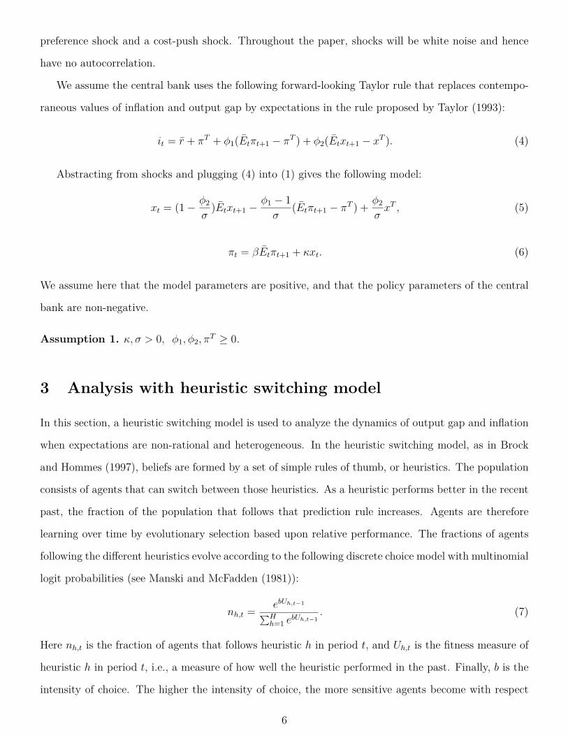
preference shock and a cost-push shock. Throughout the paper, shocks will be white noise and hence

have no autocorrelation.

We assume the central bank uses the following forward-looking Taylor rule that replaces contempo-

raneous values of inflation and output gap by expectations in the rule proposed by Taylor (1993):

it = r + πT + φ1(Etπt+1 − πT ) + φ2(Etxt+1 − xT ). (4)

Abstracting from shocks and plugging (4) into (1) gives the following model:

xt = (1− φ2

σ)Etxt+1 −

φ1 − 1σ

(Etπt+1 − πT ) + φ2

σxT , (5)

πt = βEtπt+1 + κxt. (6)

We assume here that the model parameters are positive, and that the policy parameters of the central

bank are non-negative.

Assumption 1. κ, σ > 0, φ1, φ2, πT ≥ 0.

3 Analysis with heuristic switching model

In this section, a heuristic switching model is used to analyze the dynamics of output gap and inflation

when expectations are non-rational and heterogeneous. In the heuristic switching model, as in Brock

and Hommes (1997), beliefs are formed by a set of simple rules of thumb, or heuristics. The population

consists of agents that can switch between those heuristics. As a heuristic performs better in the recent

past, the fraction of the population that follows that prediction rule increases. Agents are therefore

learning over time by evolutionary selection based upon relative performance. The fractions of agents

following the different heuristics evolve according to the following discrete choice model with multinomial

logit probabilities (see Manski and McFadden (1981)):

nh,t = ebUh,t−1∑Hh=1 e

bUh,t−1. (7)

Here nh,t is the fraction of agents that follows heuristic h in period t, and Uh,t is the fitness measure of

heuristic h in period t, i.e., a measure of how well the heuristic performed in the past. Finally, b is the

intensity of choice. The higher the intensity of choice, the more sensitive agents become with respect

6

to the relative performance of the heuristics.

We assume private sector beliefs are formed by two simple but plausible heuristics: fundamentalist

and naive. Followers of the naive heuristic make use of the high persistence in inflation and output

gap dynamics and believe future inflation or output gap to be equal to their last observed values. Note

that the naive forecast is optimal when inflation and output follow a random walk, and close to optimal

when the system contains a near unit root.

Followers of the fundamentalist heuristic, on the other hand, believe inflation and output gap to be

equal to the target values of the central bank, πT and xT , in every period. In the presence of shocks, the

central bank will not be able to achieve these targets in every period. However, since shocks are assumed

to be white noise in our model, expectations of fundamentalists coincide with rational expectations when

there are no naive agents. Fundamentalists can thus be seen to act as if all agents are rational. They

do not take into account that there are other agents in the economy, as they lack the cognitive ability

to know exactly the beliefs of other agents or the number of agents with different expectations. Since

fundamentalists believe in the long-run targets of the central bank and see these long-run values as

the best predictors for short-run future inflation and the output gap, we can interpret the fraction of

fundamentalist agents in the economy as the credibility of the central bank.

Note that we talk about the credibility of the central bank’s target values of inflation and output

gap, and not about the credibility of its future policy actions (as credibility is often referred to in the

literature). This is in line with the fact that inflation targeting can be seen as a commitment to goals

rather than a commitment to future actions and details of the CB’s operations. Credibility over targets

furthermore implicitly captures both the CB’s willingness to take actions to achieve its targets and its

ability to do so, where the latter is not straightforward in an economy with boundedly rational agents.

Finally, let the fitness measure for both variables be a weighted sum of the negative of the last

observed squared prediction error, and the previous value of the fitness measure:

U zt−1 = −(1− ρ)(zt−1 − Et−2zt−1)2 + ρU z

t−2, z = π, x, (8)

where 0 ≤ ρ ≤ 1, is the memory parameter, and E represents boundedly rational expectations of either

naive agents or fundamentalists. For analytical tractability, ρ is set to 0 for now and reintroduced in

the simulations in Section 5.

To simplify calculations and presentation, we introduce a new variable, which is defined as the

7

difference between the fraction of fundamentalist agents (nzt ) and the fraction of naive agents (1-nzt ):2

mzt = nzt − (1− nzt ) = 2nzt − 1, z = π, x. (9)

When all agents are fundamentalists, the difference in fractions equals 1, and when all agents are naive,

the difference in fractions equals −1. Henceforth we will refer to these differences in fractions simply as

fractions. These fractions can be interpreted as endogenous credibility. When mxt = mπ

t = 1, the central

bank has full credibility, and when mxt = mπ

t = −1, the CB has lost all its credibility. This credibility

measure will turn out to be very important in determining the effectiveness of monetary policy.

Using (9), aggregate expectations about inflation and output gap can be written as

Etπt+1 = (1 +mπt )

2 πT + (1−mπt )

2 πt−1, (10)

Etxt+1 = (1 +mxt )

2 xT + (1−mxt )

2 xt−1. (11)

The model is now given by (5), (6), (10), (11) and two equations for mxt+1 and mπ

t+1 that can be

obtained by combining (7), (8) and (9):

mxt+1 = Tanh

(b

2(x2t−2 − (xT )2 − 2(xt−2 − xT )xt)

), (12)

mπt+1 = Tanh

(b

2(π2t−2 − (πT )2 − 2(πt−2 − πT )πt)

). (13)

As discussed in the online appendix, this is a six-dimensional system, whose state vector can be written

as

(xt πt mx

t+2 mπt+2 mx

t+1 mπt+1

). (14)

2Note that we allow the fraction of fundamentalists, nzt , to differ between inflation and output gap (z = π, x). Agentswill then learn to use the same heuristic for both variables in times where the time series of inflation and output gap havesimilar features. However, for example, in periods of hyperinflation with an output gap close to target, agents will learnto be fundamentalist about the output gap but to use past inflation as their best predictor of future inflation. All resultspresented in this section continue to hold when it is imposed that nxt and nπt should evolve together. Results presented inSection 4 and Section 5 would also remain valid qualitatively.

8

3.1 Steady states and stability

The central bank aims to keep inflation at its target level. It would, therefore, be desirable for our

dynamical system to have a steady state with π∗ = πT . Proposition 1 states that such a steady state

indeed exists, as long as the central bank chooses an output gap target corresponding to the desired

inflation level. The proof of Proposition 1 is given in the online appendix.

Proposition 1. When the central bank sets xT = 1−βκπT , then a steady state with π∗ = πT , x∗ = xT ,

mx∗ = 0, mπ∗ = 0 exists for any value of πT .

From now on, we will assume that the central bank always chooses an output gap target consistent

with its inflation target so that the steady state where π∗ = πT and x∗ = xT exists. Since this steady

state coincides with the expectations of fundamentalists, we call this steady state the fundamental

steady state. Even though in this steady state convergence to fundamentalist expectation values has

taken place, it is not the case that all agents use the fundamentalist heuristic. This is so because the

naive heuristic also gives perfect steady state predictions, so that both fundamentalists and naive agents

have perfect foresight at the fundamental steady state. The difference in fractions, therefore, equals zero

for both variables (mx∗ = mπ∗ = 0). An intuition for this is that when the economy is stable around the

central bank’s targets, all agents have expectations close to this target, but that the reason for these

expectations differs across agents. In particular, some agents (the fundamentalists) trust the credibility

of the central bank and believe that the central bank will also be able to achieve its targets in the future.

Other agents (the naive), however, expect values close to targets only in the short run, because inflation

and the output gap were close to the targets in the recent past. When larger shocks start hitting the

economy, the first group of agents will keep believing in the targets, while the other group of agents will

start to have different expectations farther from target, in line with recent observations in the economy.

The central bank would like to achieve convergence to the fundamental steady state from as wide

a range of initial conditions as possible. This requires first of all that the fundamental steady state is

locally stable. The central bank can try to achieve stability of the fundamental steady state by choosing

the right values of the parameters in its monetary policy rule, φ1 and φ2. It turns out that the inflation

target, πT , does not matter for the stability of the fundamental steady state. Proposition 2 describes

the conditions for local stability. The results of the proposition are illustrated in Figure 1 and will be

discussed below. The proof of Proposition 2 is given in the online appendix.

9

Proposition 2. (See Figure 1) The fundamental steady state is locally stable if and only if

1− (2− β)σ + φ2

2κ = φPF1 < φ1 < φPD1 = 1 + (2 + β)3σ − φ2

2κ . (15)

At φ1 = φPF1 , a subcritical pitchfork bifurcation takes place (with two unstable, non-fundamental steady

states above the bifurcation value), with λ1 = +1. At φ1 = φPD1 , a period-doubling bifurcation takes place,

with λ2 = −1. This bifurcation is subcritical (with a 2-cycle below the bifurcation value) if φ2 < 3σ and

supercritical (with a 2-cycle above the bifurcation value) if φ2 > 3σ.

It follows from Proposition 2 that the fundamental steady state can be unstable either because the

central bank responds too weakly or because the CB responds too strongly to inflation and output gap

expectations. The intuition of instability of the fundamental steady state due to monetary policy that

reacts too weakly is the following. If period t expectations about period t+1 inflation and/or output gap

are high, and the central bank does not respond with a large enough increase in the interest rate, these

high expectations will lead to period t realizations of inflation and output gap that are even higher. This

will lead expectations about period t+ 2, formed in period t+ 1, to be higher than expectations about

period t+1, leading to even higher period t+1 realizations. This will lead to a loss of credibility for the

central bank (more agents become naive), leading to more instability. What follows is a continued rise of

both inflation and output gap, together with declining credibility: an inflationary spiral. Analogously,

for low initial conditions, a deflationary spiral will occur under weak monetary policy.

If the central bank responds too strongly to expectations, high inflation and/or output gap expecta-

tions about period t+ 1 are countered in period t by a very high interest rate. This results in very low

inflation and output gap realizations in period t, leading to very low expectations about period t + 2.

The CB then sets the interest rate very low in period t+ 1, leading to even higher inflation and output

gap realizations in period t + 1 than agents had expected. This causes a loss in credibility, and high

naive expectations about period t + 3, resulting in a high interest rate and even lower realizations in

period t+ 2 than agents expected. These cyclical dynamics continue, leading inflation and output gap

to jump up and down between ever higher and lower values, with ever declining credibility: explosive

overshooting.

[Figure 1 about here.]

The results of Propositions 1 and 2 can be combined in a bifurcation diagram. This is done in

10

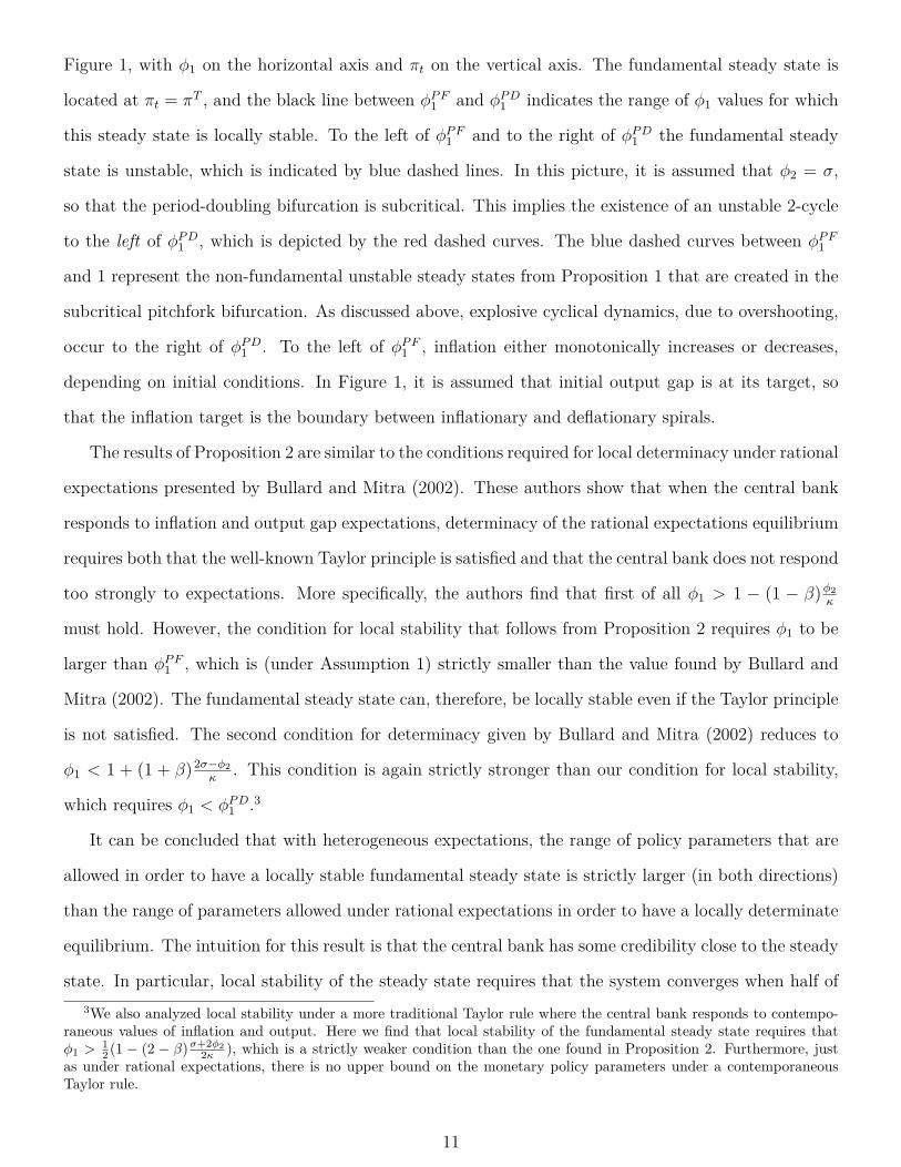
Figure 1, with φ1 on the horizontal axis and πt on the vertical axis. The fundamental steady state is

located at πt = πT , and the black line between φPF1 and φPD1 indicates the range of φ1 values for which

this steady state is locally stable. To the left of φPF1 and to the right of φPD1 the fundamental steady

state is unstable, which is indicated by blue dashed lines. In this picture, it is assumed that φ2 = σ,

so that the period-doubling bifurcation is subcritical. This implies the existence of an unstable 2-cycle

to the left of φPD1 , which is depicted by the red dashed curves. The blue dashed curves between φPF1

and 1 represent the non-fundamental unstable steady states from Proposition 1 that are created in the

subcritical pitchfork bifurcation. As discussed above, explosive cyclical dynamics, due to overshooting,

occur to the right of φPD1 . To the left of φPF1 , inflation either monotonically increases or decreases,

depending on initial conditions. In Figure 1, it is assumed that initial output gap is at its target, so

that the inflation target is the boundary between inflationary and deflationary spirals.

The results of Proposition 2 are similar to the conditions required for local determinacy under rational

expectations presented by Bullard and Mitra (2002). These authors show that when the central bank

responds to inflation and output gap expectations, determinacy of the rational expectations equilibrium

requires both that the well-known Taylor principle is satisfied and that the central bank does not respond

too strongly to expectations. More specifically, the authors find that first of all φ1 > 1 − (1 − β)φ2κ

must hold. However, the condition for local stability that follows from Proposition 2 requires φ1 to be

larger than φPF1 , which is (under Assumption 1) strictly smaller than the value found by Bullard and

Mitra (2002). The fundamental steady state can, therefore, be locally stable even if the Taylor principle

is not satisfied. The second condition for determinacy given by Bullard and Mitra (2002) reduces to

φ1 < 1 + (1 + β)2σ−φ2κ

. This condition is again strictly stronger than our condition for local stability,

which requires φ1 < φPD1 .3

It can be concluded that with heterogeneous expectations, the range of policy parameters that are

allowed in order to have a locally stable fundamental steady state is strictly larger (in both directions)

than the range of parameters allowed under rational expectations in order to have a locally determinate

equilibrium. The intuition for this result is that the central bank has some credibility close to the steady

state. In particular, local stability of the steady state requires that the system converges when half of3We also analyzed local stability under a more traditional Taylor rule where the central bank responds to contempo-

raneous values of inflation and output. Here we find that local stability of the fundamental steady state requires thatφ1 >

12 (1 − (2 − β)σ+2φ2

2κ ), which is a strictly weaker condition than the one found in Proposition 2. Furthermore, justas under rational expectations, there is no upper bound on the monetary policy parameters under a contemporaneousTaylor rule.

11

the agents believe in the target of the central bank. The central bank then only has to stabilize the

expectations of the other half of the agents, which results in weaker conditions on monetary policy. For

global stability of the steady state, it is however required that the model converges even when the system

is far away from steady state and the central bank has lost all its credibility (all naive expectations).

The conditions for that case coincide with the conditions for a locally determinate rational expectations

equilibrium. This is stated in Proposition 3, the proof of which is given in the online appendix.

Proposition 3. The fundamental steady state is globally stable when the central bank chooses

1− (1− β)φ2

κ= φGL1 < φ1 < φGU1 = 1 + (1 + β)2σ − φ2

κ. (16)

The global stability region of the fundamental steady state is indicated by the thick black line in

Figure 1. For this region of policy parameters, no unstable steady states or 2-cycles exist.

3.2 Policy implications

The difference between the local and the global stability results of the previous section highlight the

importance of the credibility of the central bank in stabilizing the economy. When the central bank is

able to retain a substantial amount of credibility, even after a sequence of bad shocks, its conditions on

monetary policy will not be very restrictive and lie close to those given in Proposition 2. In our model,

this situation would, for example, occur if the intensity of choice is not too high. If, on the other hand,

the central bank is likely to lose all its credibility after a sequence of bad shocks, the restrictions on

monetary policy lie close to those given in Proposition 3. This is in line with the results of the agent-

based model of Salle et al. (2013), who find that under low (exogenous) credibility of the central bank’s

inflation target, conditions on policy parameters are much more restrictive than under high credibility.

As in our model, the Taylor principle is furthermore not a necessary condition in the latter case.

[Table 1 about here.]

To investigate whether the stability conditions are likely to be satisfied in practice, we consider

three different parameterizations. The first two columns of Table 1 give the calibrations of σ and κ of

Woodford (1999), Clarida et al. (2000), and McCallum and Nelson (1999). Under all calibrations, the

discount factor is β = 0.99.

12

Columns 3 and 4 of Table 1 state the values of the pitchfork bifurcation (φPF1 ) and the period-

doubling bifurcation (φPD1 ), assuming that φ2 = σ. Columns 5 and 6 state the values of the global

stability restrictions given in Proposition 3. From Column 3 it follows that the pitchfork bifurcation

occurs at negative values for all calibrations. This means that, in contrast to the Taylor principle,

under these calibrations, the fundamental steady state is locally stable for monetary policy that reacts

weakly to inflation (0 < φ1 < 1) as long as φ2 = σ. This result furthermore turns out to hold for any

non-negative choice of φ2. The values of the period-doubling bifurcation (φPD1 ) given in Column 4 of

Table 1 are all unrealistically high. This means that when φ2 = σ, reacting too strongly to inflation

will not be a problem for any reasonable value of φ1. When φ2 is increased, the values of φPD1 decline.

However, even when φ2 is set to 0.375 (which corresponds to a coefficient of 1.5 when annual rather than

quarterly data are used, and which can be considered as very high), the period-doubling bifurcation

takes place at φPD1 = 7 under the Woodford (1999) calibration, and even higher values under the other

two calibrations. Hence, we can conclude that instability due to the period-doubling bifurcation only

takes place when monetary policy is extremely aggressive.

4 Zero lower bound on the nominal interest rate

In the previous section, no restrictions were placed on the values that can be taken by the nominal

interest rate. In practice, the nominal interest rate will, however, never be set negative. We will show

that if the zero lower bound (ZLB) is accounted for, the global stability result of Proposition 3 no longer

holds, but that deflationary spirals with ever decreasing inflation and output gap can arise, under any

specification of the Taylor rule. We show this in a sequence of propositions for the limiting case of

infinite intensity of choice, i.e., when all agents immediately switch to the best predictor, in Section 4.2.

In Section 4.3, we argue that for finite intensity of choice, qualitatively similar dynamics occur.

First, Section 4.1 presents a brief discussion of the existence of an extra steady state under the ZLB

under rational expectations. Section 4.2 then moves on to show that also in our model the introduction

of the ZLB can lead to the existence of an additional steady state (Proposition 4), and that the presence

of this steady state causes divergence to minus infinity for low inflation and output gap in our model,

just as in Evans et al. (2008).

Whether such a deflationary spiral occurs, however, not only depends on initial inflation and output

13

gap, but also on the credibility of the central bank (i.e., the fractions of fundamentalists). We argue

that a liquidity trap can never arise as long as the CB retains full credibility (Proposition 5), and that

a self-fulfilling deflationary spiral only arises when naive agents perform better than fundamentalists

about both variables (Proposition 6). However, even in a liquidity trap where the CB has lost all its

credibility, recovery is still possible if inflation and output gap are not too low. The deflationary spiral

and recovery regions are illustrated in Figure 2. The corresponding sufficient conditions for recovery or

a deflationary spiral to occur will be presented in Proposition 7.

Our model is capable of describing expectations-driven liquidity traps. Low initial inflation and

output gap can be interpreted as having been caused by a negative shock to the fundamentals of the

economy. Under rational expectations, the economy would immediately recover from such a shock if it

has no persistence. This is not the case in our model with heterogeneous expectations. Here it is likely

that the low realizations of inflation and output gap caused by the shock lead to a loss of credibility of

the central bank, i.e., a higher fraction of naive agents. These naive agents expect the low realizations

of inflation and output gap, and therefore the liquidity trap, to continue. These low expectations then

lead to low realizations of inflation and output gap in the next period, so that the liquidity trap indeed

continues, and expectations become self-fulfilling. If the shocks to inflation and output gap were not

too large, or if the central bank retained enough credibility, both variables will start to rise again, and

recovery to the positive interest rate region occurs. However, if expectations are too low, inflation

and output gap start to decline, resulting in more loss of credibility. The economy then ends up in a

self-fulfilling deflationary spiral with zero credibility for the central bank.

4.1 Rational expectations

It is well established that under rational expectations, the New Keynesian model with a ZLB on the

nominal interest rate has two steady states. In particular, as first highlighted by Benhabib et al.

(2001a,b), there are two combinations of a nominal interest rate and an inflation rate that satisfy the

Taylor rule with a ZLB as well as the Fisher equation, i − π = r. One of these solutions is the target

steady state, while the other steady state has a binding ZLB with i = 0 and π = −r. This second

steady state, where monetary policy is passive because the nominal interest rate cannot be set negative,

is locally indeterminate under rational expectations.

Below, we investigate whether multiple steady states also arise in our model of bounded rationality

14

when the ZLB on the nominal interest rate is introduced, and what this implies for the dynamics.

4.2 Analysis for infinite intensity of choice

When the ZLB is introduced in our model, the nominal interest rate becomes piecewise linear. In

normal times the interest rate is still given by Equation (4) and the model is as in Section 3. However,

when (4) implies that the nominal interest rate is negative, it is instead set equal to zero. We will refer

to combinations of expectations where it > 0 as the “positive interest rate region”. Combinations of

expectations that imply a binding ZLB will be referred to as the “ZLB region”. In the ZLB region, the

model is described by

xt = (1 +mxt )

2 xT + (1−mxt )

2 xt−1 + (1 +mπt )

2σ πT + (1−mπt )

2σ πt−1 + r

σ, (17)

πt = β(1 +mπ

t )2 πT + β

(1−mπt )

2 πt−1 + κxt, (18)

with fractions given by (12) and (13). The steady states of this nonlinear system depend on the fractions

of agents following the different heuristics and therefore are, in general, quite difficult to analyze. For

this reason, we first consider the limiting case where the intensity of choice equals infinity, and all

agents immediately switch to the best performing heuristic. The (six-dimensional) system then becomes

piecewise linear.

Proposition 4 states that, when the intensity of choice equals infinity, at most one (unstable) steady

state exists in the ZLB region. In this steady state, fundamentalists make persistent prediction errors,

implying that all agents have switched to naive expectations about both variables. Naive agents do not

make prediction errors, so in this steady state, expectations are perfectly self-fulfilling. The proof of

Proposition 4 is given in the online appendix.

Proposition 4. For b = +∞ there exists exactly one steady state in the ZLB region when the Taylor

principle is adhered to (φ1 > 1 − (1 − β)φ2κ

). This steady state is given by π = −r, x = −1−βκr and

mπ = mx = −1, and always is an unstable saddle point. When the Taylor principle is not adhered to

(φ1 < 1− (1− β)φ2κ

), no steady states exist in the ZLB region.

Initial conditions in the ZLB region typically will not lead to convergence to the steady state of

Proposition 4 since it is unstable. Two generic possibilities that can occur for initial conditions in the

15

ZLB region are the following. First of all, it is possible that inflation and output gap start increasing

and at some point cause the system to cross the ZLB and enter the positive interest rate region. From

then on, the dynamics will be as in Section 3. That is, for monetary policy that satisfies the conditions

of Proposition 3 (and under some additional restrictions, also policy that satisfies the conditions of

Proposition 2) convergence to the fundamental steady state occurs. The other possibility for dynamics

in the ZLB region is that inflation and output gap decline towards minus infinity. Such a deflationary

spiral can be interpreted as an inescapable liquidity trap. We will refer to the first case as “recovery”

and to the second case as “divergence” or as a “deflationary spiral”.

When the intensity of choice equals infinity, all fractions are either −1, 1 or 0. Fractions of 0

will typically only occur in a steady state and are not relevant for out-of-steady-state dynamics. This

possibility will therefore not be considered below. Four out of six state variables presented in (14) then

take on only two different values. These four state variables (fractions for inflation and output gap in

the coming two periods) can be represented by a table of 16 different combinations. This is done in

Table 2, illustrating which initial conditions lead to recovery (rather than divergence).

[Table 2 about here.]

In Proposition 5 it is stated that for the four cases in the first column of Table 2, initial fractions are

such that the system already is in the positive interest rate region from the very first period onward.

For the cases in the first row of Table 2, the system trivially is in the positive interest rate region after

one period. Therefore, it is indicated in Table 2 that for these cases recovery “Always” occurs. The

intuition behind this result is that the economy can never be in a liquidity trap when the central bank

has full credibility. Proof of Proposition 5 is given in the online appendix.

Proposition 5. If at any point in time all agents are fundamentalist about both inflation and output

gap (mπt = 1 and mx

t = 1; full credibility), recovery has occurred.

For the remaining nine cases of Table 2, recovery or divergence occurs conditional on the initial

conditions of the other two state variables: πt and xt. For most cases, it is not straightforward to define

exactly for which values of πt and xt recovery and divergence occur. However, if a deflationary spiral

occurs this must be because all agents have (negative) naive expectations about both variables after a

few periods. That is, as long as the CB retains some credibility, the economy has not (yet) entered a

16

deflationary spiral. This is stated more formally in Proposition 6, the proof of which is given in the

online appendix.

Proposition 6. A necessary condition for a deflationary spiral to occur is that at some point in time,

s ≥ t, all agents are naive with respect to both inflation and output gap for the next two periods

(mπs+1 = −1, mx

s+1 = −1, mπs+2 = −1 and mx

s+2 = −1).

From Proposition 6 it follows that a necessary condition for a deflationary spiral is that the system

at some point has moved to the bottom right entry of Table 2, with all naive expectations. This entry

is, therefore, the most interesting case when a deflationary spiral is concerned, and hence is labeled

the “deflationary spiral case”. From any other entry in Table 2 either recovery occurs, or the system

moves to the deflationary spiral case, after which the occurrence of recovery or divergence depends on

the conditions of that case. We, therefore, do not present individual conditions for all these cases, but

instead focus on the deflationary spiral case.

If, in the deflationary spiral case, initial inflation and output gap are too low, expectations will remain

naive, and output gap and inflation will keep decreasing without bound. If, however, initial inflation

and output gap are high enough, recovery occurs, either because of (positive) naive expectations, or

because at some point all agents become fundamentalists.

In Proposition 7, sufficient conditions for both recovery and divergence for the deflationary spiral case

are presented. This proposition thereby also proves that it is always possible to find initial conditions

that lead to a deflationary spiral in our model. The proof of Proposition 7 is presented in the online

appendix, and the corresponding deflationary spiral and recovery regions will be presented in Figure 2.

Proposition 7. (See Figure 2) If all agents’ expectations about both inflation and output gap are naive

for two consecutive periods (mπt+1 = mπ

t+2 = mxt+1 = mx

t+2 = −1) a sufficient condition for recovery is

that

xt > max(xev, xout), (19)

and a sufficient condition for a deflationary spiral (i.e., divergence) is that

xt < min(xev, xout, xinf ), (20)

where xev, xout, xev, xout and xinf are defined in the online appendix.

17

The above implies that for infinite intensity of choice, a deflationary spiral can always occur if initial

inflation and output gap are low enough.

The intuition for the conditions that need to be satisfied to provide a sufficient condition for a

deflationary spiral is the following. First of all, xt < xev guarantees that inflation and output gap

will keep decreasing as long as expectations about both variables remain naive (initial conditions must

lie below the stable eigenvector of the saddle point steady state). Second, xt < xout and xt < xinf

guarantee that agents do not become fundamentalists about, respectively, output gap and inflation.

Similar intuitions hold for the sufficient condition for recovery (see the proof of Proposition 7 for details).

[Figure 2 about here.]

Figure 2 plots the conditions from Proposition 7 in the (π, x)-plane for the Woodford (1999) cal-

ibration. The thick red line indicates the naive expectations ZLB for our benchmark calibration and

an annualized inflation target of 2%. This line separates the positive interest rate region from the ZLB

region. Under the above calibration, xt < xinf is always satisfied when xt < xev and xt < xout hold.

This condition is, therefore, not plotted in Figure 2. xev and xout are plotted in, respectively, solid green

and dashed black lines. For initial conditions to the left of these two lines, the sufficient conditions for a

deflationary spiral are satisfied, and inflation and output gap will keep decreasing. For initial conditions

to the right of these two lines (at least for the range of values considered in the figure), the sufficient

conditions for recovery4 are satisfied, and inflation and output gap will increase towards the positive

interest rate region.5

From the steepness of the green and dashed lines, and from the difference in scale on the axes of

Figure 2, it can be concluded that under this calibration, inflation expectations are considerably more

important than output gap expectations in determining whether recovery or divergence occurs. Similar

results are obtained under the Clarida et al. (2000) calibration.

4.3 Finite intensity of choice

Now we turn to the more general case of finite intensity of choice, where most, but not all, agents

switch to the best performing rule. Because the system is linear in fractions, consider first the other4Our “recovery region” is strongly related to the “corridor of stability” discussed in Benhabib et al. (2014) and Eusepi

(2010).5In the online appendix, it can be seen that as long as πt < πT (which is the case for the green and the dashed lines

in Figure 2), it holds that xev = xev and xout = xout.

18

limiting case where the intensity of choice is zero. Here, always half of the agents are naive, and half

are fundamentalists about each variable. Proposition 8 describes the dynamics of this system. Its proof

is given in the online appendix.

Proposition 8. Assume b = 0. If κ ≤ (2−β)σ2 , the system described by (17), (18), (12) and (13) has a

unique, stable steady state with inflation and output gap above their targets. If κ > (2−β)σ2 , the system

has an unstable saddle steady state with inflation and output gap below their targets. Furthermore, the

stable eigenvector of the system then has the same slope as that of the system with b = +∞ and all

naive expectations.

In all calibrations we consider, it holds that κ < (2−β)σ2 . It then follows from Proposition 8 that

with b = 0, all initial conditions under the ZLB lead to recovery (they are attracted to a steady state

in the positive interest rate region). When the naive heuristic is best performing, the set of initial

conditions that lead to recovery is, therefore, strictly larger when b = 0 (where half of the agents remain

fundamentalists) than when b = +∞.

In line with Proposition 6, the naive heuristic must necessarily be best performing for a deflationary

spiral to arise. Focusing on this case, the following can be concluded for finite intensity of choice.6

Since under finite intensity of choice the system is a convex combination of the systems with b = 0

and b = +∞, it follows that a lower intensity of choice leads to a larger region of initial inflation and

output gap from which recovery occurs. In that case, the lines in Figure 2 that separate the deflationary

spiral region from the recovery region are moved to the left. The intuition is that a lower intensity of

choice results in a significant fraction of fundamentalists (higher credibility), even when inflation and

output gap are low for a few periods. These fundamentalists put upward pressure on output gap and

inflation, and thereby prevent divergence for some initial conditions where a deflationary spiral would

have occurred for infinite intensity of choice. However, for lower inflation and output gap, more and

more agents become naive, so that eventually (almost) all agents are naive, just as in Section 4.2, and

deflationary spirals still arise.6Note that when the system is not in the deflationary spiral case, it may be that at some point in time fundamentalist

expectations perform better than naive expectations. In this case, a lower intensity of choice leads to fewer fundamentalists.It may then be that for some initial conditions recovery is assured in the infinite intensity of choice case, but divergenceoccurs for finite intensity of choice. This is, however, a practically less relevant case.

19

5 Monetary policy and liquidity traps

Shocks to inflation and output gap can push the economy into a liquidity trap by triggering low self-

fulfilling expectations. How can monetary policy prevent these self-fulfilling liquidity traps? In this

section, we address this question with stochastic simulations. These simulations serve two purposes.

First, they illustrate in an intuitive way how stochastic shocks can push our economy with heterogeneous

expectations and a ZLB on the nominal interest rate into an expectations-driven liquidity trap (Section

5.2). Second, we study the effectiveness of an increased inflation target and aggressive monetary easing

in preventing a liquidity trap (Section 5.3).

5.1 Calibration

Unless stated otherwise, the following parameterization is used. We follow Woodford (1999) with

κ = 0.024, σ = 0.157 and β = 0.99. We further use the policy coefficients derived by Evans and

Honkapohja (2003), φ1 = 1 + σκβµ+κ2 , φ2 = σ. Here the weight on output gap in the loss function of

the central bank is set to µ = 0.25, following McCallum and Nelson (2004) and Walsh (2003). The

policy coefficients then are given by φ1 = 1.015 and φ2 = 0.157. The inflation target is set equal to an

annualized 2%.

The shocks to output gap (ut) and to inflation (et), presented in Equations (1) and (2), are reintro-

duced in this section. Both ut and et are defined as Gaussian white noise and are calibrated to have an

annualized standard deviation of 1.1%. The calibration of the standard deviations of shocks determines

the likelihood of the occurrence of periods where the ZLB binds, as well as their severity. With the

chosen parameterization, liquidity traps do arise, but they are not so severe that no reasonable policy

measure can prevent them. We initialize the simulations at the target steady state.7 The same random

seed will be used throughout this section.

Finally, the parameters of the heuristic switching model need to be calibrated. The memory pa-

rameter in the fitness measure, (8), is set to ρ = 0.5, allowing agents to update their evaluation of the

heuristics significantly when new information arises, but also to put considerable weight on the past.8

7Different initial conditions would change the blue curves for only the first four periods or so, and the thin green curvesonly in the first period.

8We also ran all simulations in this section with ρ = 0. This only changes the result quantitatively. The policymeasures presented in Section 5.3 still work to prevent liquidity traps with a lower memory parameter, but the magnitudeof the policy change needed to achieve this is larger in that case.

20

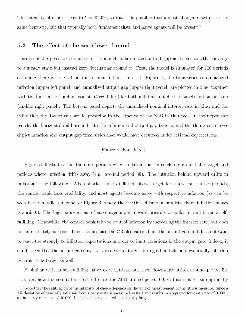
The intensity of choice is set to b = 40.000, so that it is possible that almost all agents switch to the

same heuristic, but that typically both fundamentalists and naive agents will be present.9

5.2 The effect of the zero lower bound

Because of the presence of shocks in the model, inflation and output gap no longer exactly converge

to a steady state but instead keep fluctuating around it. First, the model is simulated for 100 periods

assuming there is no ZLB on the nominal interest rate. In Figure 3, the time series of annualized

inflation (upper left panel) and annualized output gap (upper right panel) are plotted in blue, together

with the fractions of fundamentalists (Credibility) for both inflation (middle left panel) and output gap

(middle right panel). The bottom panel depicts the annualized nominal interest rate in blue, and the

value that the Taylor rule would prescribe in the absence of the ZLB in thin red. In the upper two

panels, the horizontal red lines indicate the inflation and output gap targets, and the thin green curves

depict inflation and output gap time series that would have occurred under rational expectations.

[Figure 3 about here.]

Figure 3 illustrates that there are periods where inflation fluctuates closely around the target and

periods where inflation drifts away (e.g., around period 30). The intuition behind upward drifts in

inflation is the following. When shocks lead to inflation above target for a few consecutive periods,

the central bank loses credibility, and most agents become naive with respect to inflation (as can be

seen in the middle left panel of Figure 3, where the fraction of fundamentalists about inflation moves

towards 0). The high expectations of naive agents put upward pressure on inflation and become self-

fulfilling. Meanwhile, the central bank tries to control inflation by increasing the interest rate, but does

not immediately succeed. This is so because the CB also cares about the output gap and does not want

to react too strongly to inflation expectations in order to limit variations in the output gap. Indeed, it

can be seen that the output gap stays very close to its target during all periods, and eventually inflation

returns to its target as well.

A similar drift in self-fulfilling naive expectations, but then downward, arises around period 50.

However, now the nominal interest rate hits the ZLB around period 60, so that it is set sub-optimally9Note that the calibration of the intensity of choice depends on the unit of measurement of the fitness measure. Since a

1% deviation of quarterly inflation from steady state is measured as 0.01 and results in a squared forecast error of 0.0001,an intensity of choice of 40.000 should not be considered particularly large.

21

high. This implies a high real interest rate, which depresses the output gap. Therefore, the economy

enters a recession. Furthermore, the CB loses credibility with respect to output gap as well as inflation,

implying that the economy is in the deflationary spiral case of Table 2 in Section 4.2. Moreover, inflation

and output gap have become so low that the economy is in the deflationary spiral region of Figure 2,

and inflation and output gap keep decreasing while expectations remain naive. Hence, the system has

entered a self-fulfilling deflationary spiral.

Comparing the blue curves in the top panels with the thin green curves, it can be concluded that the

drifts in inflation indeed arise because of expectations and a loss in credibility and not just because of

shocks. With the same shock sequence, rational expectations would lead both inflation and output gap

to always stay close to their targets, and the ZLB would not become binding. In the online appendix it

is shown that when the intensity of choice is set so low that credibility does not significantly change after

a sequence of positive or negative shocks, inflation and output gap remain relatively stable and close

to the rational expectations benchmark. We consider this, however, to be a less realistic calibration,

because Cornea-Madeira et al. (2017) and Branch (2004, 2007) find considerable switching between our

heuristics in inflation and survey data. In the online appendix it is further shown that for higher values

of the intensity of choice parameter, where there are larger fluctuations in credibility, similar dynamics

of inflation, output gap and the interest rate arise as in Figure 3, indicating robustness of the above

simulation.

5.3 Preventing deflationary spirals

How can the central bank prevent such a deflationary spiral? One possible solution would be to respond

with aggressive monetary easing (ME) as soon as a liquidity trap is imminent. The central bank could

set the interest rate as low as possible (i.e., zero) as soon as it would otherwise have set the interest

rate below some threshold. That is,

iMEt =

it : it ≥ TR

0 : it < TR.(21)

The threshold, TR, indicates a danger zone of a low interest rate that threatens to fall below zero.

Another possibility is increasing the inflation target, which would make it less likely that the ZLB

becomes binding and might limit how low inflation and output gap become when it does become binding.

22

This could guarantee that the system remains in the recovery region of Figure 2 and a deflationary spiral

does not occur.

It turns out that both an increased inflation target and aggressive monetary easing can indeed

prevent deflationary spirals in our simulations. Furthermore, the two measures are complements. When

there is aggressive monetary easing in place, the inflation target needs to be raised by less to prevent a

particular deflationary spiral, and vice versa.

[Figure 4 about here.]

Figure 4 illustrates that a combination of an increased inflation target and aggressive monetary

easing indeed can prevent the deflationary spiral that occurred in Figure 3. The inflation target is here

set to an annualized 2.5%, and the central bank conducts aggressive monetary easing as soon as the

annualized interest rate would have fallen below 1.5% (TR = 0.015/4).

During the period of low inflation from period 50 onward, the higher inflation target and the ag-

gressive monetary easing work together to prevent a deflationary spiral. Inflation still falls and inflation

expectations still become naive, but due to the increased inflation target, there is more room for inflation

to fall before the ZLB is hit. However, inflation does fall enough for interest rates to drop below 1.5%.

This induces the central bank to start with aggressive monetary easing by setting the interest rate to

0%, which leads to a lower real interest rate than would otherwise have occurred. As a consequence,

the output gap turns positive, which puts upward pressure on inflation, limiting the decline of inflation

even more. When, in period 58, the interest rate finally reaches the ZLB, inflation and output gap are

now high enough for the system to remain in the recovery region of Figure 2 and a deflationary spiral

does not arise. Even though inflation expectations remain naive, inflation starts to rise slowly. During

the subsequent recovery phase where the ZLB is no longer binding, the central bank keeps regularly

applying aggressive monetary easing to let inflation increase towards its target more rapidly. Eventu-

ally, both inflation and output gap are brought back to their targets, and the central bank regains its

credibility.

It must be noted, however, that the aggressive monetary easing leads to large output gap fluctuations,

which is obviously not desirable from a welfare perspective. Moreover, an increased inflation target is

generally considered to be costly as well. However, if the alternative is a long-lasting liquidity trap

and/or deflationary spiral, then these costs may be worth paying. The online appendix illustrates,

23

though, that there are also other measures that can help in preventing deflationary spirals, such as

increasing the coefficient on inflation in the Taylor rule.

6 Conclusion

A New Keynesian model is used to study inflation targeting and liquidity traps. Instead of assuming

rational expectations, we allow expectations to be formed heterogeneously by using a model where agents

switch between heuristics based on relative performance. In our model, fundamentalists, who trust the

central bank, compete with naive agents, who base their forecast on past information. The fraction of

fundamentalist agents can, therefore, be interpreted as the credibility of the central bank. Unlike in

rational expectations models, this allows us to endogenously model the central bank’s credibility, which

is of crucial importance in understanding liquidity traps.

Our first finding is that a nominal interest rate that responds too weakly or too strongly to output

gap expectations leads to instability of the fundamental steady state. In this steady state, both inflation

and output gap are equal to the targets set by the central bank. The region of policy parameters that

lead to local stability of the fundamental steady state is, however, strictly larger than the region of policy

parameters that result in a locally determinate equilibrium when rational expectations are assumed. In

fact, we find that the well-known Taylor principle is not a necessary condition for local stability in our

heterogeneous expectations model.

When the ZLB is introduced in our model, we find that expectations-driven liquidity traps can occur

for all parameterizations of the policy rule. In such a liquidity trap, the central bank has lost some,

or all, of its credibility, and low, naive expectations make the ZLB constraint binding. Whether the

economy can recover from such a liquidity trap or whether a deflationary spiral with ever decreasing

inflation and output gap occurs depends critically both on how low inflation and output gap have become

and on how much credibility the central bank is able to retain. If the central bank has lost too much

credibility, and inflation and output gap are too low, more and more agents start to coordinate on low,

naive expectations, resulting in a self-fulfilling deflationary spiral. Coordination on naive expectations

or on some other form of adaptive expectations is an empirically relevant and plausible situation that

is encountered, for example, in Assenza et al. (2014) and other laboratory experiments.

With stochastic simulations, it is shown that small shocks to the economy can lead to coordination

24

on low naive expectations, and that this can result in deflationary spirals. It is furthermore shown that

a central bank can prevent deflationary spirals by increasing the inflation target and applying aggressive

monetary easing when the interest rate becomes too low. These policy measures come, however, with

their own disadvantages and costs to the economy. Therefore, a well balanced combination of different

measures may be the best way to proceed.

25

References

Agliari, Anna, Nicolo Pecora and Alessandro Spelta (2015), ‘Coexistence of equilibria in a New Keyne-

sian model with heterogeneous beliefs’, Chaos, Solitons & Fractals 79, 83–95.

Anufriev, Mikhail, Tiziana Assenza, Cars Hommes and Domenico Massaro (2013), ‘Interest rate rules

and macroeconomic stability under heterogeneous expectations’, Macroeconomic Dynamics 17, 1574–

1604.

Arifovic, Jasmina and Luba Petersen (2015), Escaping expectations-driven liquidity traps: Experimental

evidence. Manuscript, Simon Fraser University.

Assenza, Tiziana, Peter Heemeijer, Cars Hommes and Domenico Massaro (2014), Managing self-

organization of expectations through monetary policy: a macro experiment, Technical report, CeN-

DEF Working Paper, University of Amsterdam.

Benhabib, Jess, George W. Evans and Seppo Honkapohja (2014), ‘Liquidity traps and expectation

dynamics: Fiscal stimulus or fiscal austerity?’, Journal of Economic Dynamics and Control 45, 220–

238.

Benhabib, Jess, Stephanie Schmitt-Grohe and Martin Uribe (2001a), ‘Monetary policy and multiple

equilibria’, American Economic Review 91(1), 167–186.

Benhabib, Jess, Stephanie Schmitt-Grohe and Martin Uribe (2001b), ‘The perils of Taylor rules’, Journal

of Economic Theory 96(1), 40–69.

Branch, William A. (2004), ‘The theory of rationally heterogeneous expectations: Evidence from survey

data on inflation expectations’, The Economic Journal 114(497), 592–621.

Branch, William A. (2007), ‘Sticky information and model uncertainty in survey data on inflation

expectations’, Journal of Economic Dynamics and Control 31(1), 245–276.

Branch, William A. and Bruce McGough (2010), ‘Dynamic predictor selection in a New Keynesian model

with heterogeneous expectations’, Journal of Economic Dynamics and Control 34(8), 1492–1508.

Brock, William A. and Cars H. Hommes (1997), ‘A rational route to randomness’, Econometrica:

Journal of the Econometric Society 65, 1059–1095.

26

Bullard, James and Kaushik Mitra (2002), ‘Learning about monetary policy rules’, Journal of Monetary

Economics 49(6), 1105–1129.

Busetti, Fabio, Giuseppe Ferrero, Andrea Gerali, Alberto Locarno et al. (2014), Deflationary shocks

and de-anchoring of inflation expectations, Technical report, Bank of Italy, Economic Research and

International Relations Area.

Clarida, Richard, Jordi Galı and Mark Gertler (2000), ‘Monetary policy rules and macroeconomic

stability: evidence and some theory’, Quarterly Journal of Economics 115, 147–180.

Cornea-Madeira, Adriana, Cars Hommes and Domenico Massaro (2017), ‘Behavioral heterogeneity in

U.S. inflation dynamics’, Journal of Business & Economic Statistics .

URL: https://doi.org/10.1080/07350015.2017.1321548

De Grauwe, Paul (2011), ‘Animal spirits and monetary policy’, Economic Theory 47, 423–457.

De Grauwe, Paul and Yuemei Ji (2018), ‘Inflation targets and the zero lower bound in a behavioral

macroeconomic model’, Economica .

URL: https://doi.org/10.1111/ecca.12261.

Eusepi, Stefano (2010), ‘Central bank communication and the liquidity trap’, Journal of Money, Credit

and Banking 42(2-3), 373–397.

Evans, George W., Eran Guse and Seppo Honkapohja (2008), ‘Liquidity traps, learning and stagnation’,

European Economic Review 52(8), 1438–1463.

Evans, George W. and Seppo Honkapohja (2003), ‘Expectations and the stability problem for optimal

monetary policies’, The Review of Economic Studies 70(4), 807–824.

Evans, George W. and Seppo Honkapohja (2009), ‘Learning and macroeconomics’, Annual Review of

Economics 1(1), 421–451.

Galı, Jordi (2002), New perspectives on monetary policy, inflation, and the business cycle, Technical

report, National Bureau of Economic Research.

27

Hommes, Cars, Domenico Massaro and Isabelle Salle (2018), ‘Monetary and fiscal policy design at the

zero lower bound: Evidence from the lab’, Economic Inquiry .

URL: https://doi.org/10.1111/ecin.12741

Hommes, Cars H. (2013), Behavioral rationality and heterogeneous expectations in complex economic

systems, Cambridge University Press.

Kurz, Mordecai, Giulia Piccillo and Howei Wu (2013), ‘Modeling diverse expectations in an aggregated

New Keynesian model’, Journal of Economic Dynamics and Control 37(8), 1403–1433.

Mankiw, N. Gregory, Ricardo Reis and Justin Wolfers (2003), Disagreement about inflation expecta-

tions, Technical report, National Bureau of Economic Research.

Manski, Charles F. and Daniel McFadden, eds (1981), Structural analysis of discrete data with econo-

metric applications, MIT Press Cambridge, MA.

Massaro, Domenico (2013), ‘Heterogeneous expectations in monetary dsge models’, Journal of Economic

Dynamics and Control 37(3), 680–692.

McCallum, Bennett T. and Edward Nelson (1999), Performance of operational policy rules in an esti-

mated semiclassical structural model, in ‘Monetary policy rules’, University of Chicago Press.

McCallum, Bennett T. and Edward Nelson (2004), ‘Timeless perspectives vs. discretionary monetary

policy in forward-looking models’, Federal Reserve Bank of St. Louis Review 86(2), 43–56.

Mertens, Karel and Morten O. Ravn (2014), ‘Fiscal policy in an expectations-driven liquidity trap’,

Review of Economic Studies 81(4), 1637–1667.

Milani, Fabio (2007), ‘Expectations, learning and macroeconomic persistence’, Journal of Monetary

Economics 54(7), 2065–2082.

Orphanides, Athanasios and John C. Williams (2004), Imperfect knowledge, inflation expectations, and

monetary policy, in ‘The inflation-targeting debate’, University of Chicago Press, pp. 201–246.

Orphanides, Athanasios and John C. Williams (2005), ‘Inflation scares and forecast-based monetary

policy’, Review of Economic Dynamics 8(2), 498–527.

28

Orphanides, Athanasios and John C. Williams (2007a), ‘Inflation targeting under imperfect knowledge’,

Economic Review-Federal Reserve Bank of San Francisco p. 1.

Orphanides, Athanasios and John C. Williams (2007b), ‘Robust monetary policy with imperfect knowl-

edge’, Journal of Monetary Economics 54(5), 1406–1435.

Pfajfar, Damjan and Blaz Zakelj (2018), ‘Inflation expectations and monetary policy design: Evidence

from the laboratory’, Macroeconomic Dynamics 22(4), 1035–1075.

Salle, Isabelle, Murat Yıldızoglu and Marc-Alexandre Senegas (2013), ‘Inflation targeting in a learning

economy: An abm perspective’, Economic Modelling 34, 114–128.

Taylor, John B. (1993), Discretion versus policy rules in practice, in ‘Carnegie-Rochester conference

series on public policy’, Vol. 39, Elsevier, pp. 195–214.

Walsh, Carl E. (2003), ‘Speed limit policies: the output gap and optimal monetary policy’, American

Economic Review 93, 265–278.

Woodford, Michael (1999), ‘Optimal monetary policy inertia’, The Manchester School 67(s1), 1–35.

Woodford, Michael (2003), Interest and prices: Foundations of a theory of monetary policy, Princeton

University Press.

Woodford, Michael (2004), ‘Inflation targeting and optimal monetary policy’, Federal Reserve Bank of

St. Louis Economic Review 86(4), 15–41.

29

φPF1 φGL1 φGU1 φPD1

πT

φ1

πt

DeflationarySpiral

InflationarySpiral

Locally

Stable

Globally

Stable

Locally

Stable

ExplosiveOvershooting

ExplosiveOvershooting

Figure 1: Bifurcation diagram in φ1 in case of φ2 = σ and initial output gap at steady state. The locally(globally) stable area of the fundamental steady state is indicated with a solid (thick) black line. Unstablesteady states are indicated with blue dashed curves, while the red dashed curves represent an unstable 2-cycle.When the fundamental steady state is not globally stable, explosive overshooting can occur if monetary policyis too aggressive. When monetary policy is too weak, either an inflationary or a deflationary spiral will occur.

30

−6 −4 −2 2

−25

−20

−15

−10

−5

πtxt

RecoveryDeflationary

Spiral

(πT , xT )

(πzlb, xzlb)

Figure 2: Conditions for recovery and divergence, presented in Proposition 7, for the Woodford (1999)calibration in the annualized (π, x)-plane. Here b = +∞ and mπ

t+1 = mπt+2 = mx

t+1 = mxt+2 = −1. The thick

red line indicates the ZLB for naive expectations. The black dot at 2% inflation indicates the target steadystate, while the black dot just below the ZLB depicts the unstable saddle steady state. For initial conditionsto the left of the solid green and black dashed lines, a deflationary spiral occurs. For initial conditions to theright of these two lines, recovery to the positive interest region occurs.

31

0 20 40 60 80 100−10−5

05

10

t

i t

Nominal Interest Rate (annualized)0 20 40 60 80 1000

0.20.40.60.8

1

t

nx t

Fraction Fundamentalists Output Gap

0 20 40 60 80 10000.20.40.60.8

1

nπ t

Fraction Fundamentalists Inflation0 20 40 60 80 100

−10−5

05

10

xt

Output Gap (annualized)

0 20 40 60 80 100−10−5

05

10

πt

Inflation (annualized)

Figure 3: Simulated time series. In the upper panels, the blue lines depict inflation and output in our model,the thin green lines depict time series that would have occurred under rational expectations, and the horizontalred lines depict the inflation and output gap targets. The bottom panel depicts both the actual interest rate(blue) and the rate prescribed by Equation (4) (thin red).

32

0 20 40 60 80 100−10−5

05

10

t

i t

Nominal Interest Rate (annualized)0 20 40 60 80 1000

0.20.40.60.8

1

t

nx t

Fraction Fundamentalists Output Gap

0 20 40 60 80 10000.20.40.60.8

1

nπ t

Fraction Fundamentalists Inflation0 20 40 60 80 100

−10−5

05

10

xt

Output Gap (annualized)

0 20 40 60 80 100−10−5

05

10

πt

Inflation (annualized)

Figure 4: Simulated time series in the case of an increased inflation target of 2.5% and aggressive monetaryeasing: the interest rate is set to 0 when it falls below the threshold of 1.5%. In the upper panels, the blue linesdepict inflation and output in our model, the thin green lines depict time series that would have occurred underrational expectations, and the horizontal red lines depict the inflation and output gap targets. The bottompanel depicts both the actual interest rate (blue) and the rate prescribed by Equation (4) (thin red).

33

Table 1: Parameterizations and corresponding stability conditions

Author(s) σ κ φPF1 φPD1 φGL1 φGU1

W 0.157 0.024 -5.62 20.56 0.93 14.02CGG 1 0.3 -2.367 10.97 0.97 7.63MN 1/0.164 0.3 -19.53 61.77 0.80 41.45

The first two columns of the table display the coefficients of relative risk aver-sion, σ, and the slope of the Phillips curve, κ, found by Woodford (1999), W,Clarida et al. (2000), CGG, and McCallum and Nelson (1999), MN. The finalfour columns depict the corresponding boundaries on φ1 (the coefficient on infla-tion in the Taylor rule) for local stability (φPF1 and φPD1 ) and for global stability(φGL1 and φGU1 ) that follow from Proposition 2 and 3. Here, β = 0.99 and it isassumed that φ2 = σ.

34

Table 2: Conditions for recovery for different initial conditions when b = +∞

mπt+1 = 1 mπ

t+1 = −1mxt+1 = 1 mx

t+1 = −1 mxt+1 = 1 mx

t+1 = −1mπt+2 = 1, mx

t+2 = 1 Always Always Always Alwaysmπt+2 = 1, mx

t+2 = −1 Always - - -mπt+2 = −1, mx

t+2 = 1 Always - - -mπt+2 = −1, mx

t+2 = −1 Always - - Deflationaryspiral case

When b = +∞, the fraction variables mπt+1, mx

t+1, mπt+2 and mx

t+2 take on (excluding knife edgecases) only the values −1 or 1. The table displays that for some of the 16 possible combinationsof these state variables, recovery to the positive interest region “Always” occurs. The case withmπt+1 = mx

t+1 = mπt+2 = mx

t+2 = −1 is the “Deflationary spiral case”, discussed in Proposition 6.Conditions for recovery for this case are presented in Proposition 7.

35