influence of modelling assumptions and ... columns and unsymmetrical beam capacities in the former...
TRANSCRIPT

UNIVERSITY OF LJUBLJANA Faculty of Civil and Geodetic
Engineering
Institute of Structural Engineering, Earthquake Engineering and Construction IT (IKPIR)
INFLUENCE OF MODELLING ASSUMPTIONS AND ANALYSIS PROCEDURE ON THE SEISMIC
EVALUATION OF REINFORCED CONCRETE GLD FRAMES
Aurel STRATAN and Peter FAJFAR
IKPIR Report Ljubljana, August 2002


i
ABSTRACT
Evaluation of structural response under earthquake excitation is dependent on both the characteristics of the ground motion and the assumptions considered in the analysis procedure and structure modelling. In the present study influence of some modelling options commonly assumed for nonlinear analysis of moment-resisting reinforced concrete (r.c.) frames is investigated. Emphasis is made on simple evaluation and modelling options, applied to a torsionally unbalanced gravity load designed (GLD) r.c. frame structure characteristic for older construction in Southern Europe. The structural performance is evaluated by nonlinear dynamic analyses under a set of seven bidirectional recorded ground motions. The ability of a simplified procedure (N2 method) based on nonlinear static analysis to estimate the seismic response of the torsionally unbalanced structure is investigated. Pushover analysis under different load patterns (planar and 3D), as well as two possibilities to account for bidirectional seismic input (SRSS and bidirectional load patterns) are considered in an attempt to improve the correlation with dynamic non-linear analysis. The following modelling options are investigated: rigid offsets vs. centreline dimensions of elements, bilinear, trilinear, and multilinear moment-rotation element modelling, pinching of hysteresis loops, amount of post-yielding stiffness, beam effective width, account for M-M-N interaction and strength degradation, expected vs. characteristic material strength. One-component, multispring, and fibre element models were considered. Additionally, evaluation of shear strength of members and joints according to different sources are reviewed. Displacement demands are shown to be affected significantly when the global stiffness and/or strength of the structure change. The seismic response of the analysed structure is most influenced by the bilinear vs. trilinear element modelling, rigid offsets vs. centreline element dimensions, and the consideration of M-M-N interaction and strength degradation for columns. These parameters are believed to be more important for GLD frames than for frames designed to modern codes, due to weak columns and unsymmetrical beam capacities in the former case. On the other hand, post-yielding stiffness, pinching of hysteresis loops, and beam effective width have little influence on the structural response of the investigated building. Several element models are compared to two available experimental tests on column specimens. Lumped plasticity one-component models, which do not account for strength degradation, are strongly dependent on the assumed plastic hinge length, and could provide adequate agreement with experimental results up to initiation of failure only. The distributed plasticity fibre model showed a better agreement with the two experimental tests.

iii
TABLE OF CONTENTS
ABSTRACT ............................................................................................................................................................I TABLE OF CONTENTS................................................................................................................................... III 1. INTRODUCTION ....................................................................................................................................... 1 2. THE SPEAR STRUCTURE ....................................................................................................................... 3 3. EARTHQUAKE RECORDS ...................................................................................................................... 6 4. UNCERTAINTIES IN MODELLING AND EVALUATION ................................................................. 9
4.1. MATERIALS........................................................................................................................................... 9 4.2. MODELLING OF ELEMENTS.................................................................................................................. 10 4.3. BEAM EFFECTIVE WIDTH ..................................................................................................................... 16 4.4. BEAM-COLUMN JOINTS........................................................................................................................ 20 4.5. SHEAR RESISTANCE OF MEMBERS........................................................................................................ 28 4.6. ANCHORAGE FAILURE ......................................................................................................................... 33 4.7. ROTATION CAPACITY OF ELEMENTS .................................................................................................... 34
5. STRUCTURAL MODELS AND ANALYSIS ......................................................................................... 36 5.1. GEOMETRY, LOADING, AND ANALYSIS PROCEDURE ............................................................................ 36 5.2. MODELS .............................................................................................................................................. 39 5.3. DYNAMIC CHARACTERISTICS .............................................................................................................. 41
6. INFLUENCE OF ANALYSIS PROCEDURE ........................................................................................ 43 6.1. EFFECT OF SEISMIC INPUT DIRECTION.................................................................................................. 43 6.2. EFFECT OF BIDIRECTIONAL SEISMIC INPUT .......................................................................................... 46 6.3. PUSHOVER ANALYSIS .......................................................................................................................... 56
6.3.1. Load patterns................................................................................................................................. 56 6.3.2. Influence of strength asymmetry .................................................................................................... 66 6.3.3. Bidirectional seismic input ............................................................................................................ 68
7. INFLUENCE OF MODELLING ASSUMPTIONS................................................................................ 72 7.1. BILINEAR VS. TRILINEAR ELEMENT MODELLING.................................................................................. 72 7.2. RIGID OFFSETS .................................................................................................................................... 76 7.3. POST-YIELDING STIFFNESS .................................................................................................................. 80 7.4. PINCHING ............................................................................................................................................ 83 7.5. BEAM EFFECTIVE WIDTH ..................................................................................................................... 85 7.6. M-M-N INTERACTION ......................................................................................................................... 88 7.7. STRENGTH DEGRADATION................................................................................................................... 93 7.8. EXPECTED MATERIAL STRENGTH ........................................................................................................ 96 7.9. MODELLING UNCERTAINTIES ............................................................................................................ 100
8. "BEST ESTIMATE" MODELS............................................................................................................. 102 8.1. COMPARISON TO EXPERIMENTAL TESTS ............................................................................................ 102 8.2. ONE-COMPONENT VS. FIBRE MODELS ................................................................................................ 105
9. SUMMARY AND CONCLUSIONS ...................................................................................................... 110 ACKNOWLEDGEMENTS.............................................................................................................................. 114 REFERENCES .................................................................................................................................................. 115 ANNEX I. DESCRIPTION OF THE SPEAR STRUCTURE.................................................................. 117 ANNEX II. ACCELERATION TIME-HISTORIES AND RESPONSE SPECTRA OF CONSIDERED GROUND MOTIONS ........................................................................................................... 126


Introduction 1
1. INTRODUCTION
Reinforced concrete structures in regions of low to moderate seismicity were traditionally designed for gravity loads alone, without any seismic provisions. This category of buildings are termed gravity load designed (GLD) frames, and are characteristic for buildings designed between 1930s and 1970s (Priestley, 1997), when design codes were implemented containing seismic provisions more or less equivalent to those currently in practice. Though local design practices and codes were different in different geographical areas, this problem is common to many regions, such as USA (Kunnath et al., 1995), New Zealand (Park, 2002), and Europe (Cosenza et al., 2002, Calvi et al., 2002). The main deficiencies in reinforced concrete GLD frames are related to poor detailing and lack of capacity design, leading to reduced local and global ductility. The following are the typical features of GLD frames (Aycardi et al., 1994, Priestley, 1997, Cosenza et al., 2002): Columns are weaker than the adjacent beams, leading to a storey mechanism. Minimal transverse reinforcement in columns for shear and confinement,
particularly in the plastic hinge zones. Frequently, transverse reinforcement is anchored with 90° bends in the cover concrete. Large spacing and inadequate anchorage lead to spalling of compression concrete, buckling of longitudinal reinforcement and collapse of the plastic hinge regions.
Little or no transverse reinforcement in beam-column joints, resulting in a high potential for joint shear failure.
Discontinuous positive (bottom) beam longitudinal reinforcement in the beam-column joints.
Lap splices located in potential plastic hinge zones just above the floor slab levels.
Plain reinforcing bars for longitudinal reinforcement, that leads to early loss of bond and increases deformations in the structure.
Inclined reinforcement for shear resistance in beams, that is not effective for shear reversals.
Lack of structural regularity in plan and/or elevation, further worsening the seismic response due to torsion and storey mechanisms.
Evaluation of seismic response of reinforced concrete structures is subjected to considerable degree of approximation and simplification of the "real" behaviour. A very sophisticated structural modelling for design purposes is seldom necessary, as detailing of elements based on experimental investigations and their response in past earthquakes, as well as capacity design principles assures the validity of a considerable number of simplifications in the structural model. However, assessment of seismic response of existing GLD structures based on usual assumptions in modelling of r.c. structures may be inappropriate. Additional issues of varying degree of sophistication should be addressed in order to assess the behaviour of poorly detailed GLD buildings. The available sources of information needed for evaluation of structural response of a building are design codes (e.g. Eurocode 2, Eurocode 8), evaluation guidelines for existing buildings (e.g. FEMA 356), and scientific publications. Design codes are intended primarily for design of new buildings, and therefore are based on some assumptions and simplifications characteristic for appropriately detailed members. In addition, they are generally very conservative and therefore are often not appropriate for prediction of structural response of existing structures. Evaluation guidelines are expected to provide a better, though sometimes much simplified and prescriptive

Introduction 2
approach. Information that can be grasped from professional literature is usually scattered and difficult to compile into a single and clear procedure. This study addresses the investigation of the influence of different simplifications, assumptions and uncertainties in modelling of structural elements and the structure as a whole on the seismic response of GLD r.c. buildings. Emphasis is made on simple evaluation and modelling options, that can be readily performed with existing software packages. The structural response is assessed by nonlinear dynamic (time-history) analysis, and the ability of the N2 method (Fajfar, 2000) based on nonlinear static (pushover) analysis to estimate the seismic response is explored.
The SPEAR structure 3
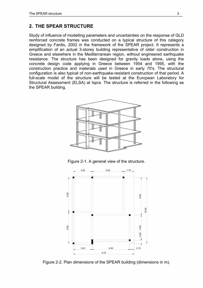
2. THE SPEAR STRUCTURE
Study of influence of modelling parameters and uncertainties on the response of GLD reinforced concrete frames was conducted on a typical structure of this category designed by Fardis, 2002 in the framework of the SPEAR project. It represents a simplification of an actual 3-storey building representative of older construction in Greece and elsewhere in the Mediterranean region, without engineered earthquake resistance. The structure has been designed for gravity loads alone, using the concrete design code applying in Greece between 1954 and 1995, with the construction practice and materials used in Greece in early 70's. The structural configuration is also typical of non-earthquake-resistant construction of that period. A full-scale model of the structure will be tested at the European Laboratory for Structural Assessment (ELSA) at Ispra. The structure is referred in the following as the SPEAR building.
Figure 2-1. A general view of the structure.
10.5
0
6.00
4.00
0.50
5.50
5.00
9.70
6.003.00 0.70
5.003.00 1.70
Figure 2-2. Plan dimensions of the SPEAR building (dimensions in m).

The SPEAR structure 4
Dimensions in plan of the structure are presented in Figure 2-2. The storey height is 3 m, with 2.5 m clear height of columns between the beams. The specified design strength of concrete is fc=25 N/mm2, and the design yield strength of reinforcement is fy=320 N/mm2. Design gravity loads on slabs are 0.5 kN/m2 for finishings and 2 kN/m2 for live loads. Slab is 150 mm thick, cast in place monolithically, and reinforced with 8 mm bars at 200 mm. Columns longitudinal reinforcement is composed of 12 mm plain bars, lap spliced over 400 mm at each floor level, including the first level. Spliced bars have 180° hooks. Column stirrups are 8 mm plain bars at 250 mm centres, closed with 90° hooks (see Figure 2-3), and they do not continue into the joints. Typical beam longitudinal reinforcement is shown in Figure 2-3 and Figure 2-4. It is composed of two 12 mm bars at the top, anchored with 180° hooks at the far end of the column. The bottom beam reinforcement consists of two 12 mm bars anchored at the far end of the column with 180° hooks, and other two 12 mm bars that are bent up towards the supports. The latter are anchored with downward bends into the joint core at exterior joints, and continue into the next span at interior joints. Additional longitudinal reinforcement, as well as bars of greater diameter (20 mm) are used for some heavier loaded beams (B4,18,32, B7,21,35, B9,23,37). Beam stirrups are 8 mm bars at 200 mm centres, anchored with 90° hooks. A complete description of the structure is presented in Annex I.
750
250
250
250
15
15
250x250 columns
250x750 columns
4Ø12
Ø8/250
Ø8/250
10Ø12250
15
Ø8/200
2Ø12
4Ø12Ø8/200
Ø8/200
150
350 50
0
typical beam
Figure 2-3. Typical beam and column cross-sections (dimension in mm).
Figure 2-4. Typical beam longitudinal reinforcement.

The SPEAR structure 5
The main deficiencies of the structure could be summarised as follows: use of plain reinforcing bars slender columns (250x250), with largely spaced stirrups inclined reinforcement in beams for shear resistance and optimal distribution of
reinforcement column lap splices in potential plastic hinge zones lack of shear reinforcement in beam-column joints inadequate anchorage of stirrups (90° hooks) irregular plan layout

Earthquake records 6
3. EARTHQUAKE RECORDS
Seven ground motion records from Southern Europe were selected (see Table 3-1) from the European strong motion databank (Ambraseys et al., 2000). The selection of records was based on criteria of magnitude (at least 5.8), peak ground acceleration (at least 1.5 m/s2), and conformity to the Eurocode 8 spectrum. The basic characteristics of the records are presented in Table 3-2.
Table 3-1. Earthquake records used in this study.
Earthquake name Date Station name Record
abbr. Alkion 24.02.1981 Korinthos - OTE Building AL1 Alkion 24.02.1981 Xilokastro - OTE Building AL2 Campano Lucano 23.11.1980 Calitri CA1
Kalamata 13.09.1986 Kalamata – Prefecture KA1 Kalamata 13.09.1986 Kalamata - OTE Building KA2 Montenegro 15.04.1979 Ulcinj - Hotel Albatros MO1 Montenegro 15.04.1979 Bar - Skupstina Opstine MO2
Table 3-2. Characteristics of the earthquake records.
Record Surface - wave magnitude (Ms)
Epicentral distance
Soil category PGA, m/s2 Scaling
factor AL1 6.7 20km soft soil 2.26 (X), 3.04 (Y) 1.074 AL2 6.7 19km alluvium 2.84 (X), 1.67 (Y) 0.937 CA1 6.9 16km stiff soil 1.53 (X), 1.73 (Y) 0.813 KA1 5.8 9km stiff soil 2.11 (X), 2.91 (Y) 0.791 KA2 5.8 10km stiff soil 2.35 (X), 2.67 (Y) 1.047 MO1 7.0 21km Rock 1.78 (X), 2.20 (Y) 0.991 MO2 7.0 16km stiff soil 3.68 (X), 3.56 (Y) 0.388
Scaling of the ground motion records was performed in order to bring them to the same level of seismic intensity. Eurocode 8 (2002) acceleration elastic response spectrum was used as the target spectrum (PGA=0.2g, soil parameter S=1, TB=0.2s, TC=0.6s, TD=2.0s, 5% damping). Three-dimensional nonlinear dynamic analysis requires bidirectional records (vertical component was ignored in this study). It was decided not to alter the ratio of intensities between the two components. Therefore, the procedure suggested in FEMA 356, (2000) was used here. It involves construction of the Square Root of Sum of Squares (SRSS) spectrum from the two horizontal components of each record, and applying the scaling procedure to the SRSS target spectrum (one-directional EC8 spectrum times 2 ). Scaling procedure was applied for each record separately, by minimizing the error function. The error function was defined as the difference between the areas under the SRSS spectrum of a record and the SRSS of the target spectrum in the period range between TC and TD. The fundamental period of vibration of the structure is situated in this range. The mean of SRSS spectra of scaled records, the mean plus/minus standard deviation, and the target SRSS spectrum are shown in Figure 3-1.

Earthquake records 7
0 1 2 3 40
2
4
6
8
10
12
T, s
SA
, m/s
2
SRSS OF SCALED RECORDS
EC8MEANMEAN + STDMEAN − STD
Figure 3-1. Mean of the Square Root of Sum of Squares (SRSS) of scaled records
and the target EC8 spectrum.
0 1 2 3 40
1
2
3
4
5
6
7
8
T, s
SA
, m/s
2
X COMPONENTS SCALED
EC8MEANMEAN + STDMEAN − STD
Figure 3-2. Mean of the X components of scaled records and the target EC8
spectrum. The applied scaling procedure assures a uniform intensity of seismic input near the fundamental period of the structure, and enables a direct comparison of the results from nonlinear dynamic analyses to the simplified pushover (N2) method. Mean of individual X and Y components of the records are presented in Figure 3-2 and Figure 3-3. A reasonable fit to the target EC8 spectrum could be observed in this case also. Acceleration time histories of the scaled records, as well as elastic response spectra of individual scaled and unscaled records are presented in Annex II.

Earthquake records 8
0 1 2 3 40
2
4
6
8
10
T, s
SA
, m/s
2
Y COMPONENTS SCALED
EC8MEANMEAN + STDMEAN − STD
Figure 3-3. Mean of the Y components of scaled records and the target EC8
spectrum.

Uncertainties in modelling and evaluation 9
4. UNCERTAINTIES IN MODELLING AND EVALUATION
4.1. Materials
There is a general agreement that design (characteristic) strength is not appropriate for evaluation of existing buildings (Priestley, 1997) for two reasons. First is that use of design strength is too conservative, and the second is that the use of characteristic instead of expected strength for concrete may often lead to change of predicted failure mode from ductile flexure to brittle shear. Ideally, expected strengths of concrete and steel are to be determined experimentally. In the absence of experimental tests, different values are suggested in literature (see Table 4-1). In the same table are presented the ultimate strains specified in the same sources. Design codes (EC2) provide the most conservative estimates (as would be expected). However, there is an important difference between the other two "predictive" oriented sources in the case of steel strength and ultimate strain. Table 4-1. Relation between characteristic and expected strength for materials, and
ultimate strain limits.
EC2 Priestley FEMA 356 Concrete compression strength (fc)
fck + 8 N/mm2 (1.3 fck for C25/30) 1.5 fck 1.5 fck
Steel yield strength (fy) - 1.1 fyk 1.25 fyk Ultimate concrete strain (bending) 0.0035 0.005 0.005
Ultimate steel strain - 0.10-0.15 0.02 – compr. 0.05 - tension
where: fck – concrete characteristic (nominal) compression strength; fyk – steel characteristic yield strength. Concrete strength and ultimate strain could be further enhanced by the effect of confining. However, this will seldom be the case for poorly detailed GLD frames. According to Priestley (1997), concrete should be considered unconfined if the following conditions govern: stirrups ends not bent back into the core, and spacing of stirrups in the potential plastic hinge is such that: s≥d/2 or s≥16dbl
where s is the stirrups spacing, d is the effective depth of the cross section, and dbl is the diameter of the longitudinal reinforcement. For the SPEAR building, these requirements will imply unconfined conditions for both beams and columns. Analytical modelling of steel will be usually based on an elastic-perfectly plastic stress-strain relationship. Strain hardening may be considered for a more realistic behaviour of steel in tension. A refined modelling of steel in compression will require accounting for buckling of longitudinal reinforcement. Lower ultimate steel strains in compression in the FEMA 356 approach may be intended to account in an approximate way for the effect of reinforcement buckling. Modelling of concrete in compression will usually consist of a parabola stress-strain relationship up to a strain of approximately 0.002, with a plastic plateau afterwards, up to the ultimate strain (0.0035 – 0.005). A more realistic modelling, especially for the case of unconfined concrete, is to consider the softening (descending) branch after the attainment of the maximum strength.

Uncertainties in modelling and evaluation 10
Three models of steel and concrete stress-strain relationships were considered in this study (see Figure 4-1). The first one is the "design" model (D), based on characteristic strengths, bilinear steel, and parabola-rectangle stress-strain relationship for concrete in compression. The second one (DD) is based on the design strengths, but strain hardening is included for steel and degradation for concrete in compression. The softening branch of concrete stress-strain relationship is the one of Kent & Park, described in Penelis and Kappos (1997). The third model (E) is based on expected material strengths (Priestley approach), strain hardening steel and degrading concrete.
Table 4-2. Material characteristics.
Model D DD E Concrete compression strength (fc)
25 N/mm2 25 N/mm2 37.5 N/mm2 (1.5 fck)
Steel yield strength (fy) 320 N/mm2 320 N/mm2 352 N/mm2 (1.1 fyk)
Ultimate concrete strain 0.0035 0.0050 (at 0.2fc) 0.0037 (at 0.2fc)
Ultimate steel strain 0.10 0.05 0.05
0
100
200
300
400
500
0 0.025 0.05 0.075 0.1
STRAIN
STR
ESS,
N/m
m2
DDDE
0.0
5.0
10.0
15.0
20.0
25.0
30.0
35.0
40.0
0 0.002 0.004 0.006
STRAIN
STR
ESS,
N/m
m2
D
DD
E
Figure 4-1. Stress-strain models for steel and concrete.
4.2. Modelling of elements
Modelling of nonlinear behaviour of r.c. frames may be performed in different ways, ranging from finite element models of increased complexity, to models based on macroelements representing structural members (beams and columns), or even bigger portions of a structure. Nonlinear analysis models based on macroelements for beams and columns are widely used due to reliability and computational efficiency. A variety of implementations for modelling reinforced concrete elements exist, depending on the computer code used. Several element modelling options available in CANNY 99 (Li, 2002) program were considered in this study. Behaviour of moment-resisting frames is governed by the flexural response of beams and columns. One of the simplest models for flexural behaviour of beam-column is the one-component model (Figure 4-2a). All inelastic deformations are assumed concentrated at elements end (lumped plasticity model). The element is characterised by a bilinear or trilinear moment-rotation envelope curve, and a set of

Uncertainties in modelling and evaluation 11
rules describing cyclic behaviour. Two one-component elements are necessary to model a column in biaxial bending. It offers a great flexibility in modelling, by allowing for such effects as stiffness and strength degradation, and pinching under cyclic loading. However, the CANNY implementation of the model is strictly correct only for elements in double curvature with the inflexion point located at the mid length of the member, and it does not account for axial force-moment (M-N) and biaxial moment (M-M) interaction. Also, tuning of the parameters describing cyclic behaviour may be difficult to accomplish when experimental data is missing. A variant of one-component model implemented in CANNY is moment-curvature based model, assuming linear variation of flexibility along the member. This model is appropriate for members with moment distribution close to the uniform one. The same limitations of the moment-rotation based one-component model apply. The multi-spring model (see Figure 4-2b) is composed of an elastic line element and two multi-spring elements at each end. Each multi-spring element consists of a number of springs (fibres) representing uniaxial behaviour of concrete or steel materials. The model accounts naturally for biaxial moments and axial force (M-M-N) interaction. The multi-spring element is considered to be of zero length in establishing member force-displacement relationship (being a lumped plasticity model in effect). The force-deformation relationship of the multi-spring element itself is determined based on a plastic zone length and the Bernoulli plane section assumption.
(a) (b)
Figure 4-2. One-component model (a) and multi-spring model (b), (Li, 2002). A distributed plasticity model is available in the CANNY program as well. It is based on discretisation of cross-sections at the element ends into a number of fibres, similarly to the multi-spring model. However, a linear variation of curvature along the element is assumed, resulting in a distributed plasticity model. Like the multispring model, the fibre model accounts naturally for the interaction of biaxial moments and axial force. Several models for flexural behaviour were considered in this study: bilinear (B) and trilinear (T) one-component models, lumped plasticity multi-spring (MS), and distributed plasticity fibre (F) models. Shear and torsional behaviour were assumed elastic in all cases.

Uncertainties in modelling and evaluation 12
The bilinear moment-rotation relationship for elements was modelled based on the procedure described in Paulay and Priestley, 1992 (see Figure 4-3). A standard moment-curvature analysis was carried out for each element. For columns, axial force corresponding to gravitational loading was considered. Yield curvature yφ was determined at first yielding of reinforcement or at the attainment of 0.0015 strain in concrete. The ultimate curvature uφ was found at attainment of ultimate steel or concrete strains, as discussed in chapter 4.1. The equivalent plastic hinge length was determined as:
0.08 0.022p b yL L d f= ⋅ + ⋅ ⋅ (4-1)
where L is the shear span of the member (assumed half the clear span for most of the members), db is the diameter of the longitudinal reinforcement, and fy is the yield strength of the reinforcement. Then, the moment-rotation relationship is obtained by integrating the curvature distribution along the element length:
/ 3y y Lθ φ= ⋅ (4-2)
( ) ( )θ θ φ φ
⋅ − ⋅= + −
0.5p pu y u y
L L LL
(4-3)
where yθ is the yield rotation and uθ is the ultimate rotation.
Sample bilinear idealisations of the moment-curvature and moment-rotation relationships for the C3 column and the beams B1 and B5 used for the DB model (see chapter 5.2) are presented in Figure 4-4.
Figure 4-3. Equivalent curvatures and plastic hinge length for bilinear model
(Paulay and Priestley, 1992) A slightly modified procedure was used for constructing the trilinear moment-curvature and moment-rotation relationships (see Figure 4-5 and Figure 4-6). Cracking curvature cφ was defined as the one corresponding to the attainment of the lower cracking moment Mc in the cross section. The yield curvature yφ and moment My were determined by a numerical procedure based on a significant reduction of the slope to the moment-curvature curve. This is a more general procedure that the one based on first yield in reinforcement or attainment of a predefined strain in concrete. The ultimate curvature uφ was determined as previously at the attainment of ultimate strains in concrete or steel. With the plastic hinge length defined as in equation (4-1), the following relations were used to derive the trilinear moment-rotation relationship:

Uncertainties in modelling and evaluation 13
/ 3c c Lθ φ= ⋅ (4-4)
1 1 26
c c cy c y
y y y
M M MLM M M
θ φ φ
= ⋅ ⋅ + + ⋅ − ⋅ + (4-5)
( ) ( )θ θ φ φ
⋅ − ⋅= + −
0.5p pu y u y
L L LL
(4-6)
0
10
20
30
40
50
60
0 0.01 0.02 0.03 0.04 0.05
CURVATURE, 1/m
MO
MEN
T, k
Nm
C3bilinear
0
10
20
30
40
50
60
0 0.005 0.01 0.015
ROTATION, radM
OM
ENT,
kN
m
C3-bilinear
0
10
20
30
40
50
60
70
80
0 0.05 0.1 0.15 0.2 0.25
CURVATURE, 1/m
MO
ME
NT,
kN
m
B1i, B5ij-POSB1i, B5ij-NEG
0
10
20
30
40
50
60
70
80
0 0.01 0.02 0.03 0.04
ROTATION, rad
MO
MEN
T, k
Nm B1i, B5ij-POS
B1i, B5ij-NEG
(a) (b)
Figure 4-4. Sample bilinear idealisation of the moment-curvature relationship (a) and the derived moment-rotation relationship (b) for the DB model.
M
φc
c yM
φc
cM
φy
MuMcMy
L L
φc
yφ
Lp
uφ
Figure 4-5. Curvature distribution along the shear span
for trilinear moment-curvature idealisation.

Uncertainties in modelling and evaluation 14
0 0.01 0.02 0.03 0.04 0.050
20
40
60
CURVATURE, 1/m
MO
ME
NT
, kN
m
C3C3−TRI
0 0.002 0.004 0.006 0.008 0.01
0
20
40
60
ROTATION, rad
MO
ME
NT
, kN
m
C3−TRI
0 0.05 0.1 0.15 0.2 0.250
20
40
60
80
CURVATURE, 1/m
MO
ME
NT
, kN
m
B1I, B5IJ−POSB1I, B5IJ−NEG
0 0.01 0.02 0.03 0.04
0
20
40
60
80
ROTATION, rad
MO
ME
NT
, kN
m
B1I, B5IJ−POSB1I, B5IJ−NEG
Figure 4-6. Sample trilinear idealisation of the moment-curvature relationship (a) and
the derived moment-rotation relationship (b) for the DT model. In the case of the multi-spring element, the element cross-section was discretised into steel and concrete springs, as in Figure 4-8. Material stress-strain curves presented in Figure 4-1 were used. The plastic zone length was assumed equal to the equivalent plastic hinge length defined by equation (4-1). The same cross-section discretisation and material models were used for the fibre model, plastic hinge length definition being unnecessary in this case, however.
0.0
5.0
10.0
15.0
20.0
25.0
30.0
35.0
40.0
0 0.002 0.004 0.006
STRAIN
STR
ESS,
N/m
m2
CoreCover
0.0
5.0
10.0
15.0
20.0
25.0
30.0
35.0
40.0
0 0.002 0.004 0.006
STRAIN
STR
ESS,
N/m
m2
CoreCover
DD E
Figure 4-7. Stress-strain models for core and cover concrete for DD and E concrete models.

Uncertainties in modelling and evaluation 15
2502
2
4
750
4
250
37
35
33
31
29
27
25
23
12
10
24
2
19
15
11
822
28
32
36
18
27
31
35
14
26
30
3420 33
16 29
12 25
106
250
X
3882818079
3678777675
3474737271
3270696867
3066656463
2862616059
2658575655
24545352
9
X
51
16 18 20 22 146
49
47
45
43
41
39
11
8
31
3
17
2340
21
39
17
38
135 9
24 37
Y5
50106105104103
4810210110099
4698979695
4494939291
4290898887
4086858483
7
3
Y
15 17 19 21 135
1
13
4
Figure 4-8. Discretisation of column cross-sections for the multi-spring and fibre
elements. In the case of bilinear element modelling, a simplification often used is the assumption of an effective element flexural stiffness as a fixed ratio of the uncracked stiffness. Eurocode 8 stipulate an effective stiffness of 0.5EcIg for both beams and columns, where Ec is the concrete modulus of elasticity, and Ig is the gross moment of inertia of the element cross-section. Other sources recognize the stiffening effect of compressive axial load on columns, differentiating effective stiffness as a function of column axial load. Thus, FEMA356 specifies effective stiffness of 0.5EcIg for beams, 0.7EcIg for columns with a nondimensional axial compressive force ν≥0.5Agfc, and 0.5EcIg for columns with ν≤0.3Agfc. Paulay and Priestley (1992), recommend values of 0.35EcIg for beams, 0.8EcIg for columns with a nondimensional axial compressive force ν>0.5Agfc, and 0.6EcIg for columns with ν<0.2Agfc. For the SPEAR structure, EC8 and FEMA 356 lead to the same effective stiffness of 0.5EcIg for beams and columns, as the level of compressive axial force in columns was ν≤0.3Agfc. The Paulay and Priestley approach would provide more flexible beams and stiffer columns, as compared to the EC8/FEMA356 approach. The simplified modelling of initial effective stiffness for the DBCS model was based on the values provided by EC8/FEMA356, as both amounted to the same values considering the level of axial force in columns (ν≤0.3Agfc). Analytical predictions of the secant stiffness for bilinear models DB and DBC (design characteristics of materials, EC8 effective beam widths) ranged from 0.10EcIg to 0.26EcIg for beams, 0.17EcIg to 0.37EcIg for 250x250 columns, and 0.14EcIg to 0.19EcIg for 250x750 columns, with average values of 0.14EcIg, 0.24EcIg, 0.17EcIg,

Uncertainties in modelling and evaluation 16
respectively. In the case of beams, the average of positive and negative bending stiffness was assumed for bilinear modelling. Another simplification in modelling of r.c. elements, especially when effective stiffness is used, is the assumption of empirical values of post-yielding stiffness for the moment-rotation relationship. Some commonly used values are about 1% to 3% of the secant stiffness to the yield point. FEMA356 recommends strain hardening values ranging from 0% to 10%. Sometimes higher values were found to fit well the experimental results. Thus, Dolsek and Fajfar (2002) used 10% post-yielding stiffness for beams under positive bending (bottom reinforcement in tension) and columns, and 20% for beams under negative bending. Higher values of strain hardening for beams under negative bending are intended to approximately account for the observation of increase of the flange effective width as the plastic deformations increase. Average analytical predictions of post-yielding stiffness values for the bilinear models DB and DBC were of 0.46% and 1.64% for beams under positive and negative bending respectively, 1.70% for 250x250 columns, and 2.11% for 250x750 columns. Due to the different procedure used to determine the yield curvature and moment, and the ultimate rotation, in the case of the trilinear models DT and DTC average values of analytical strain hardening amounted to 0.56% and 0.86% for beams under positive and negative bending respectively, 1.8% for 250x250 columns, and 3.4% for 250x750 columns.
4.3. Beam effective width
Slab contribution to the strength and stiffness of beams could be important for the seismic assessment of r.c. frames, as it will affect the relative beams/columns strength and stiffness. This, in effect may change the plastic mechanism. However, this contribution is difficult to estimate, as it varies along the length of the member, and depends on the level of inelastic deformations, as well as presence of transverse beams and anchorage of the slab reinforcement (Paulay and Priestley, 1992). Thus, the effective flange width specified in codes and literature is only an approximate measure of the real and complex slab contribution. Several approaches for determination of effective slab width are considered in the following. Eurocode 8 (2002) states that the effective flange width beff is drastically reduced due to local plastification effects. The effective width values provided are intended for determination of member strength (not stiffness). The following relations are suggested: a) for beams framing into exterior columns: Bc – in the absence of a transverse beam 4c fB h+ ⋅ – if there is a transverse beam of similar dimension
b) for beams framing into interior columns: the above lengths may be increased by 2hf on each side of the beam
where: Bc – column width, hf – slab height Eurocode 2 (2001) states that in T beams the effective flange width, over which uniform conditions of stress can be assumed, depends on the web and flange dimensions, the type of loading, the span, the support conditions and the transverse reinforcement. Values of effective widths are intended for all limit states (strength and stiffness) and are to be based on the distance L0 between points of zero moments:

Uncertainties in modelling and evaluation 17
,eff eff i wB B B B= + ≤∑
with , 0 00.2 0.1 0.2eff i iB B L L= ⋅ + ⋅ ≤ ⋅ and ,eff i iB B≤
where Beff is the flange effective width on each side of the web; Bi is the half the clear distance to the next beam web; Bw is the beam web width. FEMA 356 specifies that for flanged beams the combined stiffness and strength for flexural and axial loading shall be calculated considering a width of effective flange on each side of the web equal to the smaller of: the provided flange width, eight times the flange thickness, half the distance to the next web, or one-fifth of the span for beams.
The New Zealand seismic provisions NZS3101 consider that flange contribution to stiffness in T and L beams is typically less than the contribution to flexural strength, as a result of the moment reversals occurring across beam-column joints and the low contribution of tension flanges to flexural stiffness. Consequently, it is recommended that for load combinations including seismic actions, the effective flange contribution to the stiffness be 50% of that commonly adopted for gravity load strength design (Paulay and Priestley, 1992). The following effective widths are specified for determination of stiffness: for T beams, Beff is the lesser of: Bw+ 8hf Bw+ Lny/2 Lx/8
For L beams Bw+ 3hf Bw+ Lny/4 Bw + Lx/24
where: Lx – span length of beam; Lny – clear distance to the next web. Paulay and Priestley, (1992) recommend that in T and L beams, built integrally with the floor slabs, the longitudinal slab reinforcement placed parallel with the beam, to be considered effective in participating as beam tension (top) reinforcement. In addition to the bars placed within the web width of the beam, these should include all bars within the effective width in tension Beff, which may be assumed to be the smallest of the following: ¼ of the span of the beam under consideration, extending each side from the
centre of the beam section, where a flange exists ½ of the span of a slab, transverse to the beam under consideration, extending
each side from the centre of the beam section, where a flange exists ¼ of the span length of a transverse edge beam, extending each side of the
centre of the section of that beams which frames into an exterior column and is thus perpendicular to the edge of the floor
Within this width Beff only those bars in the slab that can develop their tensile strength at or beyond a line of 45° from the nearest column should be relied on. At edge beams, effective anchorage of bars, in both the top and bottom of the flange must also be checked. Where no beam is provided at the edge of a slab, only those slab bars that are effectively anchored in the immediate vicinity of a column should be relied on (Beff=2 Bc).

Uncertainties in modelling and evaluation 18
hf
Beff
Bw Beff,2Beff,i
Lb
B1 B2
Beff
Bw (Bc)
Figure 4-9. Notations used for definition of effective flange width.
A comparison of the different approaches in determining beam effective widths is presented in Table 4-3. The same notations (see Figure 4-9) were used to facilitate the comparison. It can be observed that different approaches disagree on whether the effective widths should be used for determination of strength, stiffness or both. Eurocode 8 provide similar values with NZS3101, but these values are intended for strength in the first case and stiffness in the second one. Higher effective widths (and close to each other) are specified by FEMA 356 and Paulay and Priestley. A comparison of beam effective widths in the case of the SPEAR structure is presented in Figure 4-10. Though the predictions are close in the case of short span beams, the differences (up to three times) become important for larger span beams.
0 1000 2000 3000
B1
B2
B3
B4
B5
B6
B7
B8
B9
B10
B11
B12
Bea
m N
o.
Effective width, end i, mm
EC2EC8P&PFEMA
0 1000 2000 3000
B1
B2
B3
B4
B5
B6
B7
B8
B9
B10
B11
B12
Bea
m N
o.
Effective width, end j, mm
EC2EC8P&PFEMA
Figure 4-10. Comparison of beam effective widths of SPEAR structure.

Uncertainties in modelling and evaluation 19
Table 4-3. Comparison of effective flange widths according to different approaches.
T beams L beams Remarks EC8 Beff = BC+ Beff,1 + Beff,2
a) for beams framing into exterior columns: Beff,i ≤ 2 hf Beff,i = 0 in the absence of a transverse beam b) for beams framing into interior columns: Beff,i ≤ 4 hf
for bending resistance
EC2 Beff = Bw+ Beff,1 + Beff,2 Beff,i ≤ 0.5 Bi Beff,i ≤ 0.2 Bi + 0.05 LB Beff,i ≤ 0.1 LB
for all limit states; L0 – distance between points of zero moments; L0 assumed LB/2
FEMA 356 Beff = Bw+ Beff,1 + Beff,2 Beff,i ≤ 8 hf Beff,i ≤ 0.5 Bi Beff,i ≤ 0.2 LB
for both stiffness and strength
Paulay and Priestley
Beff = Bw+ Beff,1 + Beff,2 in the absence of a transverse beam: Beff = 2BC Beff,i ≤ 0.5 Bi Beff,i ≤ 0.25 LB – Bw/2 Beff,i ≤ 0.25 (Bi + Bw) for beams framing into exterior columns
for effective tension reinforcement (negative bending)
NZS 3101 (Paulay and Priestley)
Beff = Bw+ Beff,1 + Beff,2 Beff,i ≤ 4 hf Beff,i ≤ 0.25 Bi Beff,i ≤ 0.0625 LB – Bw/2
Beff = Bw+ Beff,1 Beff,i ≤ 3 hf Beff,i ≤ 0.25 Bi Beff,i ≤ 0.0417 LB
for stiffness analysis; 50% of the values specified for strength design under gravity loading (flange in compression)
Table 4-4. Stiffness, strength and ductility properties of B9 beam, end j.
Beff, mm Moment of inertia, m4
Yield moment, kNm
Ultimate curvature, 1/m
EC8 550 4375.4x10-6 + 37.2 - 128.3
+ 0.184 - 0.079
FEMA 356 2650 6120.7x10-6 + 38.9 - 181.5
+ 0.205 - 0.048

Uncertainties in modelling and evaluation 20
0 0.05 0.1 0.15 0.2 0.250
50
100
150
200
CURVATURE, 1/m
MO
ME
NT
, kN
m
EC8
B9J−POSB9J−NEG
0 0.05 0.1 0.15 0.2 0.25
0
50
100
150
200
CURVATURE, 1/m
MO
ME
NT
, kN
m
FEMA 356
B9J−POSB9J−NEG
Figure 4-11. Influence of effective width variation for beam B9, end j.
When assessing the beam flexural resistance under negative moments (top reinforcement in tension), only the top slab reinforcement effectively anchored was considered. Yield strength of beam longitudinal reinforcement with insufficient anchorage was adjusted as described in chapter 4.6. Influence of the beam effective width on the moment-curvature relationship can be observed in Figure 4-11 and Table 4-4, for the "design" assumptions for material model (D). The 4.8 times increase of beam effective width has the major consequence of increasing the negative yield moment (by 40%). Approximately the same increase is accomplished for the section moment of inertia. Positive yield moment (bottom bars in tension) is basically unaffected by the increase in effective flange width. Yield curvature is basically the same for both assumptions. The ultimate negative curvature (controlled by crushing of compressed concrete) decreases with increase of the effective width, due to reduction of the neutral axis depth. The ultimate positive curvature, however, may increase for a larger effective width, as the failure mode changes from crushing of concrete to attainment of ultimate steel strains in bottom reinforcement.
4.4. Beam-column joints
There are two major problems in the beam-column joints of GLD frames. The first one is related to the insufficient bond between the longitudinal reinforcement and the concrete core, due to relatively small depth of the columns. This is of concern especially in the interior joints, were the slip of plain top bars may be significant. If significant slip occurs, the bar will be in tension through the joint core, and the compression reinforcement at one side of the column may be actually in tension. This was shown to result in reduction of the beam ductility and strength (Hakuto et al., 1999), in addition to a reduction of the frame stiffness. The second problem is related to the assessment of the shear behaviour of the joints, which lack transverse reinforcement. Shear failure of beam-column joint cores without transverse reinforcement is due to extensive diagonal tension cracking that may eventually lead to diagonal compression failure in the joint core (Hakuto et al., 2000). Attempts have been made to predict the shear failure of the joints by limiting the nominal stress vjh as a function of concrete compressive strength (fc), tensile strength ( cf ), or by limiting the principal compression and tensile stresses in the joint. Two mechanisms of shear resistance are traditionally considered (Paulay and Priestley, 1992): the diagonal strut mechanism and the truss mechanism. The latter is ineffective in the case of joints lacking transverse reinforcement or after bond deterioration between the beam longitudinal reinforcement and the joint core.

Uncertainties in modelling and evaluation 21
Consequently, the shear resistance of GLD frames beam-column joints will rely on the diagonal strut mechanism only (see Figure 4-12).
Mb1Mb2
Vc
Figure 4-12. Concrete diagonal strut mechanism in interior bam-column joints.
In the case of exterior beam-column joints, the extent to which the diagonal compression strut mechanism can be mobilised depends greatly on the detailing of longitudinal beam reinforcement. Longitudinal beam reinforcement bent into the joint core (see Figure 4-13a) will permit the diagonal compression strut to bear effectively against the bend, since the bearing stresses at the bend of the bar act in the direction of the strut. When beam reinforcement is bent away from the joint (see Figure 4-13b), diagonal strut in the joint can not be stabilized, and joint failure occurs at an early stage (Priestley, 1997).
(a) (b)
Figure 4-13. Mechanism of shear transfer in exterior beam-column joints. The horizontal shear force acting on the joint can be written as (Hakuto et al., 2000):
1 2
1 2
b bjh c
b b
M MV Vz z
= + − (4-7)
where: Mb1 and Mb2 are the beam moments at the face of the joints core; zb1 and zb2 are the lever arms between the tensile forces and the centroids of compressive forces, Vc is the shear force in the column above the joint.

Uncertainties in modelling and evaluation 22
The nominal shear stress at the mid-depth of the column can be written as:
/jh jh jv V A= (4-8)
where Aj = bj hc is the effective cross sectional area of the joint core; bj – effective width of the joint core; hc – column depth. The nominal axial compressive stress in the column at the mid-depth of the joint core can be written as:
/a jf N A= (4-9)
where N – axial compressive load on the column above. Both vjh and fa stresses are nominal values, as they are not uniform over the joint core. Though the stress distribution in the joint core is not elastic, a measure of the principal tensile (pt) and compressive (pc) stresses in the joint could be derived from the Mohr's circle (compression positive):
2
2
2 2a a
c jhf fp v = + +
(4-10)
2
2
2 2a a
t jhf fp v = − +
(4-11)
Eurocode 8 (2002) draft provides the following formula to ensure that "the diagonal compression induced in the joint by the diagonal strut mechanism does not exceed the compressive strength of concrete in the presence of transverse tensile strains" in the case of interior joints:
1 djh cv f ν
ηη
≤ ⋅ − (4-12)
where: 0.6 (1 / 250)cfη = ⋅ − , fc in N/mm2; νd – normalised axial force in the column above. In the case of exterior joints, 80% of the value provided by (4-12) is required. FEMA 356 (2000) defines the joint shear strength as:
jh cv fλ γ≤ ⋅ (4-13)
in which λ = 0.75 for lightweight aggregate concrete and 1.0 for normal weight aggregate concrete, and γ is as defined in Table 4-5. In addition to classification of beam-columns joints as interior or exterior, FEMA 356 distinguishes another category of knee joints.
Table 4-5. Values of γ for Joint Strength Calculation, for fc in N/mm2, and ρ"<0.003, FEMA 356, (2000)
Interior joint with transverse beams
Interior joint without transverse beams
Exterior joint with transverse beams
Exterior joint without transverse beams
Knee joint
1.0 0.83 0.66 0.50 0.33
ρ" - volumetric ratio of horizontal confinement reinforcement in the joint; knee joint = self-descriptive (with transverse beams or not).

Uncertainties in modelling and evaluation 23
Priestley (1997) suggested a failure model for interior joints based on the principal compression stress:
2
2 (0.45...0.5)2 2a a
c jh cf fp v f = + + ≤ ⋅
(4-14)
where: 0.5c cp f= ⋅ for one way joints, and 0.45c cp f= ⋅ for two-way joints to allow for the effects of the biaxial joint shear. The joint strength decreases with imposed ductility demand, according to the model in Figure 4-14a. Equation (4-14) can be rearranged as:
1 ajh c
c
fv pp
≤ − (4-15)
where pc takes values between 0.45 (at 0.0 plastic drift) and 0.225 (at 0.04 plastic drift) for two-way joints. For exterior beam-column joints, the joint shear strength is expressed as a function of the principal tensile stress pt:
2
2 (0.29...0.42)2 2a a
t jh cf fp v f = − + ≤ ⋅
(4-16)
with limiting values of 0.29t cp f= − ⋅ for beam bars bent away from the joint, and
0.42t cp f= − ⋅ for beam bars bent into the joint. The above values reduce with increasing drift demand, as in Figure 4-14b. Equation (4-16) can be rearranged as:
1 ajh t
t
fv pp
≤ − (4-17)
0
0.1
0.2
0.3
0.4
0.5
0 0.01 0.02 0.03 0.04 0.05
plastic drift
pc/f c
one-way jointstwo-way joints
00.05
0.10.15
0.20.25
0.30.35
0.40.45
0 0.01 0.02 0.03 0.04 0.05
joint rotation [drift]
pt/ √
f c
beam bars bentinto jointbeam bars bentaway from joint
(a) (b)
Figure 4-14. Strength degradation models for exterior (a), and interior (b) joints, (Priestley, 1997)

Uncertainties in modelling and evaluation 24
0
0.05
0.1
0.15
0.2
0 2 4 6 8
displacement ductility factor, µ
v jh/f
c
Figure 4-15. Model for degradation of joint strength with imposed ductility demand,
Hakuto et al., 2000 Hakuto et al. (2000) experimentally studied the shear strength of interior beam-column joints without shear reinforcement and found that the nominal joint shear stress increases almost proportional to the compressive strength of concrete. The following equation was proposed:
0.17jh cv f≤ ⋅ (4-18)
with joint shear strength degradation with increasing ductility demand as in Figure 4-15, Kitayama et al. (1991) suggested a limit of 0.25fc for the joint shear stress in order to prevent shear failure of interior beam-column joints after beam yielding. Also, it was found that the presence of transverse beams and slab improve the shear strength of the joint approximately 1.3 times, a limit of 0.33fc being suggested in this case. Non-dimensional column axial stress smaller than 0.5 cf⋅ was found not to affect the joint shear strength. In the case of exterior beam column joints with plain bars anchored by 180° hooks, Pampanin et al. (2001) found that this particular joint detail may lead to premature joint degradation. The principal tensile stress limitation 0.2t cp f= ⋅ was suggested as the upper limit for first diagonal cracking, followed by "significant and sudden strength reduction without any additional source for hardening behaviour".
Figure 4-16. Failure mode of exterior beam column joints with 180° hooked bars,
Pampanin et al., 2001.

Uncertainties in modelling and evaluation 25
A typical arrangement of reinforcement in the beam-column joints of the SPEAR building is presented in Figure 2-4. Bottom beam bars at the column face (two φ12 in general) end at the far end of the column with 180° hooks. The same applies for two φ12 "montage" bars at the top of the beams in the case of exterior joints, while the remaining bars are adequately anchored by bents into the joint core. This joint configuration can not be strictly assigned to any of the descriptions found in literature on which available shear strength models are based. However, the joint shear stress associated with positive bending moments (bottom bars in tension) will be lower than the one associated with negative bending moment (top bars in tension), due to the low amount of bottom reinforcement, associated with possible pullout. As part of the top beam reinforcement is adequately bent into the joint core, it is believed that it will be sufficient for the development of the compression strut mechanism, so that the limitation 0.42t cp f= − ⋅ suggested by Priestley (1997) for this category of joints, can be adopted. In the case of interior beam-column joints, the arrangement of the beam reinforcement is not so important due to presence of beams on both sides of the joints.
Table 4-6. Joint shear strength vjh,Rd for the x direction, N/mm2 (values for high ductility demand in parentheses)
Joint ID
Joint type EC8 FEMA356 Priestley Hakuto
J1-x int. 12.1 4.6 9.9 (4.1) 4.3 (1.3) J2-x ext. 9.8 2.9 3.1 (1.2) - J3-x ext. 8.8 3.3 3.7 (1.6) - J4-x ext. 9.4 2.9 3.4 (1.4) - J5-x ext. 10.4 2.9 2.5 (0.8) - J6-x int. 12.2 4.6 9.9 (4.2) 4.3 (1.3) J7-x ext. 10.2 2.9 2.7 (1.0) - J8-x ext. 10.5 2.9 2.4 (0.8) - J9-x ext. 10.0 3.3 2.9 (1.1) - J10-x int. 12.8 4.6 10.6 (4.9) 4.3 (1.3) J11-x ext. 10.3 2.9 2.6 (0.9) - J12-x ext. 9.8 3.3 3.0 (1.2) - J13-x ext. 10.1 2.9 2.8 (1.0) - J14-x ext. 10.6 2.9 2.3 (0.7) - J15-x int. 12.9 4.6 10.6 (5.0) 4.3 (1.3) J16-x ext. 10.5 2.9 2.4 (0.8) - J17-x ext. 10.7 2.9 2.2 (0.6) - J18-x ext. 10.4 3.3 2.5 (0.9) - J19-x int. 13.5 4.6 11.3 (5.6) 4.3 (1.3) J20-x ext. 10.8 1.7 2.1 (0.5) - J21-x ext. 10.8 1.7 2.1 (0.5) - J22-x ext. 10.8 1.7 2.1 (0.5) - J23-x ext. 10.8 1.7 2.1 (0.5) - J24-x int. 13.5 4.6 11.3 (5.6) 4.3 (1.3) J25-x ext. 10.8 1.7 2.1 (0.5) - J26-x ext. 10.8 1.7 2.1 (0.5) - J27-x ext. 10.8 1.7 2.1 (0.5) -
A comparison of different approaches in computing the shear resistance of beam-column joints of the SPEAR building is presented in Table 4-6 and Table 4-7. The

Uncertainties in modelling and evaluation 26
level of axial force in the column, where required, was considered the one from the gravity loads only (no earthquake forces). In the case of FEMA356 approach, the tabulated γ values were interpolated for the case of transverse beams framing into one side of the joint only. The 0.45c cp f= ⋅ limitation of the principal compression stress and the 0.42t cp f= − ⋅ limitation of the principal tensile stress were considered for the Priestley approach in the case of interior and exterior joints respectively. When the joint shear capacity was defined in terms of the principal tensile or compression stresses, the relations (4-15) and (4-17) were used to derive the equivalent shear stress expression. It can be observed that the joint shear strength predictions according to different approaches differ sometimes by more than 100%. The EC8 joint shear capacity is the most unconservative one for both interior and exterior joints. FEMA356 predictions are in good agreement with Priestley values for exterior joints, and with Hakuto values for interior joints (for low ductility demands). However, the capacity of interior joints according to Priestley approach are roughly twice those of FEMA 356 or Hakuto et al.
Table 4-7. Joint shear strength vjh,Rd for the y direction, N/mm2 (values for high ductility demand in parentheses)
Joint ID
Joint type EC8 FEMA356 Priestley Hakuto
J1-y ext. 9.7 3.3 3.1 (1.2) - J2-y ext. 9.8 2.9 3.1 (1.2) - J3-y int. 11.0 4.6 8.7 (2.5) 4.3 (1.3) J4-y ext. 9.4 2.9 3.4 (1.4) - J5-y ext. 10.4 2.9 2.5 (0.8) - J6-y ext. 9.7 2.5 3.1 (1.2) - J7-y ext. 10.2 2.9 2.7 (1.0) - J8-y ext. 10.5 2.9 2.4 (0.8) - J9-y int. 12.5 4.6 10.2 (4.5) 4.3 (1.3)
J10-y ext. 10.3 3.3 2.7 (0.9) - J11-y ext. 10.3 2.9 2.6 (0.9) - J12-y int. 12.3 4.6 10.0 (4.3) 4.3 (1.3) J13-y ext. 10.1 2.9 2.8 (1.0) - J14-y ext. 10.6 2.9 2.3 (0.7) - J15-y ext. 10.3 2.5 2.6 (0.9) - J16-y ext. 10.5 2.9 2.4 (0.8) - J17-y ext. 10.7 2.9 2.2 (0.6) - J18-y int. 13.0 4.6 10.8 (5.1) 4.3 (1.3) J19-y ext. 10.8 1.7 2.1 (0.5) - J20-y ext. 10.8 1.7 2.1 (0.5) - J21-y int. 13.5 4.6 11.3 (5.6) 4.3 (1.3) J22-y ext. 10.8 1.7 2.1 (0.5) - J23-y ext. 10.8 1.7 2.1 (0.5) - J24-y ext. 10.8 1.7 2.1 (0.5) - J25-y ext. 10.8 1.7 2.1 (0.5) - J26-y ext. 10.8 1.7 2.1 (0.5) - J27-y int. 13.5 4.6 11.3 (5.6) 4.3 (1.3)

Uncertainties in modelling and evaluation 27
Demand to Capacity Ratios (DCR) of the joint shear stresses of the DT model, mean of dynamic analyses under 0.2 g earthquakes are presented in Table 4-8 and Table 4-9. Despite the important variation of DCR predictions according to different models, it is little probability that they will represent a weak link in the SPEAR structure. Some joints (J3-x and J21-x) may approach their strength according to FEMA 356 model. The interstorey drift demand for the 0.2 g intensity set of earthquakes is of the order of 0.01 rad, so that the joint strength in the case of Priestley and Hakuto et al. approaches will be characterised by the upper values (low ductility demands, see Figure 4-14 and Figure 4-15).
Table 4-8. Joint DCR for the x direction, DT model, 0.2 g (values for high ductility demand in parentheses)
Joint ID
Joint type EC8 FEMA356 Priestley Hakuto
J1-x int. 0.20 0.53 0.25 (0.59) 0.57 (1.94) J2-x ext. 0.20 0.68 0.64 (1.62) - J3-x ext. 0.36 0.95 0.85 (1.99) - J4-x ext. 0.26 0.85 0.73 (1.77) - J5-x ext. 0.15 0.53 0.61 (1.80) - J6-x int. 0.08 0.22 0.10 (0.24) 0.23 (0.79) J7-x ext. 0.18 0.64 0.68 (1.88) - J8-x ext. 0.14 0.49 0.59 (1.83) - J9-x ext. 0.19 0.57 0.64 (1.68) - J10-x int. 0.14 0.41 0.17 (0.37) 0.44 (1.48) J11-x ext. 0.15 0.54 0.59 (1.70) - J12-x ext. 0.24 0.71 0.77 (1.98) - J13-x ext. 0.20 0.69 0.71 (1.92) - J14-x ext. 0.12 0.44 0.56 (1.89) - J15-x int. 0.07 0.19 0.08 (0.17) 0.20 (0.68) J16-x ext. 0.11 0.40 0.48 (1.51) - J17-x ext. 0.11 0.39 0.51 (1.80) - J18-x ext. 0.15 0.46 0.60 (1.78) - J19-x int. 0.07 0.21 0.08 (0.17) 0.22 (0.76) J20-x ext. 0.06 0.42 0.33 (1.40) - J21-x ext. 0.15 0.98 0.77 (3.23) - J22-x ext. 0.08 0.55 0.43 (1.81) - J23-x ext. 0.06 0.41 0.32 (1.34) - J24-x int. 0.04 0.10 0.04 (0.08) 0.11 (0.38) J25-x ext. 0.05 0.34 0.27 (1.13) - J26-x ext. 0.05 0.33 0.26 (1.08) - J27-x ext. 0.08 0.50 0.39 (1.63) -

Uncertainties in modelling and evaluation 28
Table 4-9. Joint DCR for the y direction, DT model, 0.2 g (values for high ductility
demand in parentheses)
Joint ID
Joint type EC8 FEMA356 Priestley Hakuto
J1-y ext. 0.23 0.67 0.70 (1.78) - J2-y ext. 0.24 0.81 0.76 (1.93) - J3-y int. 0.30 0.72 0.38 (1.30) 0.77 (2.63) J4-y ext. 0.23 0.75 0.64 (1.57) - J5-y ext. 0.12 0.43 0.50 (1.48) - J6-y ext. 0.07 0.27 0.22 (0.55) - J7-y ext. 0.20 0.69 0.73 (2.02) - J8-y ext. 0.16 0.59 0.71 (2.20) - J9-y int. 0.16 0.44 0.19 (0.44) 0.47 (1.59)
J10-y ext. 0.17 0.53 0.66 (1.85) - J11-y ext. 0.18 0.64 0.71 (2.03) - J12-y int. 0.21 0.57 0.26 (0.60) 0.61 (2.07) J13-y ext. 0.16 0.57 0.59 (1.59) - J14-y ext. 0.10 0.37 0.47 (1.58) - J15-y ext. 0.09 0.35 0.33 (0.94) - J16-y ext. 0.17 0.61 0.73 (2.30) - J17-y ext. 0.14 0.53 0.69 (2.43) - J18-y int. 0.13 0.36 0.15 (0.32) 0.39 (1.32) J19-y ext. 0.09 0.56 0.44 (1.84) - J20-y ext. 0.09 0.56 0.44 (1.84) - J21-y int. 0.10 0.29 0.12 (0.24) 0.32 (1.07) J22-y ext. 0.10 0.66 0.52 (2.17) - J23-y ext. 0.06 0.36 0.28 (1.19) - J24-y ext. 0.08 0.56 0.44 (1.83) - J25-y ext. 0.10 0.63 0.50 (2.09) - J26-y ext. 0.10 0.65 0.51 (2.16) - J27-y int. 0.07 0.20 0.08 (0.16) 0.22 (0.74)
4.5. Shear resistance of members
Shear failure of reinforced concrete members is of brittle type therefore it is avoided in the design of new structures. The shear capacity of beams and columns of GLD frames may be insufficient due to the following reasons: columns often have only nominal transverse reinforcement, with spacing similar to
column dimensions beam shear reinforcement is usually in the form of inclined bars, that do not
provide a resisting mechanism at load reversal stirrups may not be adequately anchored with 135° hooks, their efficiency being
reduced in this case Shear capacity of reinforced concrete members is known to depend on the degree of flexural ductility in the plastic hinge. A distinction can be made between a brittle shear failure of columns before the flexural strength of the column has been reached,

Uncertainties in modelling and evaluation 29
and ductile shear failure, where a degree of ductility develops in plastic hinges before shear failure occurs (Priestley et al., 1994). Evaluation of shear strength by the code equations may be excessively conservative in many cases. In the following shear strength evaluation by EC8/EC2, FEMA 356, and Priestley et al. approaches are compared. Eurocode 8 (2002) draft refers to Eurocode 2 for shear design of reinforced concrete elements in moment-resisting frames, specifying that the inclination θ in the truss method is specified to be 45°. The contribution of concrete to the shear strength is given in Eurocode 2 (2001) draft as:
( )1/ 30.18 100 0.15c l c cp wV k f b dρ σ = ⋅ ⋅ ⋅ ⋅ − ⋅ ⋅ ⋅ (4-19)
with a minimum of 0.4 0.15c ct cp wV f b dσ = ⋅ − ⋅ ⋅ ⋅ , and where: = + ≤1 200 / 2k d ;
ρ =⋅sl
lw
Ab d
; / 0.2cp c cN A fσ = > ⋅ ; fc - concrete compressive strength; d – effective
depth of the member, Asl – area of the tensile reinforcement effectively anchored, bw – cross-section width, N – axial force in the cross section, Ac – area of concrete cross-section. The shear resistance for members with vertical shear reinforcement is taken as the lesser off:
cotsws yw
AV z fs
θ= ⋅ ⋅ ⋅ and νθ θ⋅ ⋅ ⋅
=+max cot tan
w cRd
b z fV (4-20)
Contribution of the inclined shear reinforcement is taken as the lesser off:
(cot cot ) sinswsi yw
AV z fs
θ α α= ⋅ ⋅ ⋅ + ⋅ and θ ανθ
+= ⋅ ⋅ ⋅ ⋅
+max 2cot cot
1 cotRd w cV b z f (4-21)
where: Asw – cross-sectional area of the shear reinforcement, s – spacing of stirrups, fyw – yield strength of shear reinforcement, z - inner lever arm corresponding to the maximum bending moment ( 0.9z d≅ ⋅ ), θ - angle between the concrete compression struts and the main tension chord; 0.6 (1 / 250)cfν = ⋅ − ; α - angle between shear reinforcement and the main tension chord. However, according to Eurocode 2 (2001) draft, the contribution of concrete to the member shear strength is to be disregarded if it is insufficient in resisting the shear force alone, for both beams and columns. While this approach may be a reasonable simplification for design needs, it is definitely not appropriate for evaluation purposes. FEMA 356 provides the following comments on the evaluation of shear strength of members: Within yielding regions of components with low ductility demands and outside
yielding regions for all ductility demands, calculation of design shear strength using procedures for effective elastic response such as the provisions in Chapter 11 of ACI 318 shall be permitted.
Where the longitudinal spacing of transverse reinforcement exceeds the component effective depth measured in the direction of shear, transverse reinforcement shall be assumed ineffective in resisting shear or torsion.
For beams and columns in which perimeter hoops are either lap-spliced or have hooks that are not adequately anchored in the concrete core, transverse reinforcement shall be assumed not more than 50% effective in regions of

Uncertainties in modelling and evaluation 30
moderate ductility demand and shall be assumed ineffective in regions of high ductility demand.
In the case of beams (where low ductility demands are expected), the ACI 318 applies for the contribution of concrete (with fc in N/mm2):
0.166c c wV f b d= ⋅ ⋅ ⋅ (4-22)
In the case of columns, the following equation is provided by FEMA 356 (with fc in N/mm2) for the contribution of concrete:
0.5
1 (0.8 )/( ) 0.5
cc w
c c
f NV k b hM V d f A
λ ⋅ = ⋅ ⋅ + ⋅ ⋅ ⋅ ⋅ ⋅ ⋅
(4-23)
in which k = 1.0 in regions of low ductility demand, 0.7 in regions of high ductility demand, and varies linearly between these extremes in regions of moderate ductility demand; λ = 0.75 for lightweight aggregate concrete and 1.0 for normal weight aggregate concrete; N = axial compression force (= 0 for tension force); M/V is the largest ratio of moment to shear under design loadings for the column; M/(V d) shall not be taken greater than 3 or less than 2; d is the effective depth; and Ac is the gross cross-sectional area of the column. It shall be permitted to assume d = 0.8h, where h is the dimension of the column in the direction of shear. The steel contribution is given as:
sw ys
A f dV
s⋅ ⋅
= (4-24)
(sin cos )y ys
A f dV
sα α
⋅ ⋅= ⋅ + (4-25)
for stirrups, and inclined reinforcement, respectively. Priestley et al. (1994) proposed a predictive model of the shear strength of the column considering it to consist of three independent components: a concrete component Vc whose magnitude depends on the level of ductility, an axial load component Vp whose magnitude depends on the column aspect ratio, and a truss component Vs whose magnitude depends on the transverse reinforcement content.
Rd c p sV V V V= + + (4-26)
with the three components evaluated as:
0.8c c gV k f A= ⋅ ⋅ ⋅ (4-27)
k=0.29 for member displacement ductility 1θµ ≤ (biaxial), or curvature ductility 1ϕµ ≤ ; k=0.1 for member displacement ductility 3θµ ≥ (biaxial), or curvature ductility 5ϕµ ≥ ; k varies linearly between member displacement ductility 1 and 3 (see Figure 4-17).
2p
h cV Pa−
= (4-28)
h – the overall section depth; c – the depth of the compression zone; a = L for a cantilever column, and a = L/2 for a column in reversed bending.

Uncertainties in modelling and evaluation 31
cot30sw yws
A f dV
s⋅ ⋅
= ⋅ ° (4-29)
Asw – the total transverse reinforcement area per layer; fyw – the steel yield strength; s – spacing of stirrups; d – the effective depth
Figure 4-17. Degradation of concrete shear strength with ductility, Priestley et al.,
(1994) The model of Priestley et al. (1994) was developed for column sections. The following adjustments have been proposed for evaluation Vc in the case of beams (Priestley, 1997): k=0.2 for member displacement ductility 1θµ ≤ (biaxial), or curvature ductility 1ϕµ ≤ ; k=0.05 for member displacement ductility 3θµ ≥ (biaxial), or curvature ductility 5ϕµ ≥ ; k varies linearly between member displacement ductility 1 and 3. A comparison of the shear capacities for the SPEAR building computed according to the three approaches presented above are given in Table 4-10. In the case of the EC2/EC8 approach, if the code prescriptions are to be taken ad literam, the shear strength is to be computed from the contribution of steel only. In addition, the 45° inclination of θ in the truss model would imply no contribution of the stirrups for the shear strength of 250x250 columns, due to their large spacing (s = 250 mm). Therefore, both steel and concrete contributions to the shear strength were considered, except for 250x250 column and 250x750 columns in the weak (x) direction, where stirrups are ineffective in resisting shear. For beams, two shear capacities were computed, corresponding to negative bending (
RdVM − ) when the
inclined reinforcement is effective, and corresponding to positive bending (Rd
VM+ ), when the inclined reinforcement is ineffective. The following equations apply: For EC2/EC8 approach: beams:
RdVM
c s siV V V− = + + , Rd
VMc sV V+ = +
250x250 column and 250x750 column in the weak (x) direction: Rd
V cV=
250x750 column in the strong (y) direction: Rd
V c sV V= +
For FEMA 356 approach (stirrups contribution reduced to 50% due to inadequate anchorage):
Uncertainties in modelling and evaluation 32
beams: Rd
V 0.5Mc s siV V V− = + ⋅ + ,
RdV 0.5M
c sV V+ = + ⋅
250x250 column and 250x750 column in the weak (x) direction: Rd
V cV=
250x750 column in the strong (y) direction: Rd
V 0.5c sV V= + ⋅
For Priestley et al. (1994, 1997) approach (steel component was included for all columns due to the 30° angle between the shear reinforcement and the tension chord in this model): beams:
RdVM
c s siV V V− = + + , Rd
VMc sV V+ = +
columns: Rd
V c s pV V V= + +
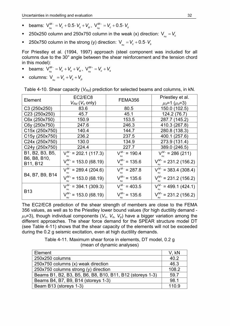
Table 4-10. Shear capacity (VRd) prediction for selected beams and columns, in kN.
Element EC2/EC8 VRd (Vs only) FEMA356 Priestley et al.
µθ=1 (µθ=3) C3 (250x250) 83.6 80.5 150.0 (102.5) C23 (250x250) 45.7 45.1 124.2 (76.7) C6x (250x750) 150.9 153.5 287.7 (145.2) C6y (250x750) 247.6 246.3 410.3 (267.8) C15x (250x750) 140.4 144.7 280.8 (138.3) C15y (250x750) 236.2 237.5 400.1 (257.6) C24x (250x750) 130.0 134.9 273.9 (131.4) C24y (250x750) 224.4 227.7 389.0 (246.5) B1, B2, B3, B5, B6, B8, B10, B11, B12
RdVM − = 202.1 (117.3)
RdVM+ = 153.0 (68.19)
RdVM − = 190.4
RdVM+ = 135.6
RdVM − = 286 (211)
RdVM+ = 231.2 (156.2)
B4, B7, B9, B14 RdVM − = 289.4 (204.6)
RdVM+ = 153.0 (68.19)
RdVM − = 287.8
RdVM+ = 135.6
RdVM − = 383.4 (308.4)
RdVM+ = 231.2 (156.2)
B13 RdVM − = 394.1 (309.3)
RdVM+ = 153.0 (68.19)
RdVM − = 403.5
RdVM+ = 135.6
RdVM − = 499.1 (424.1)
RdVM+ = 231.2 (156.2)
The EC2/EC8 prediction of the shear strength of members are close to the FEMA 356 values, as well as to the Priestley lower bound values (for high ductility demand - µθ=3), though individual components (Vc, Vs, Vp) have a bigger variation among the different approaches. The shear force demand for the SPEAR structure model DT (see Table 4-11) shows that the shear capacity of the elements will not be exceeded during the 0.2 g seismic excitation, even at high ductility demands.
Table 4-11. Maximum shear force in elements, DT model, 0.2 g (mean of dynamic analyses)
Element V, kN 250x250 columns 40.2 250x750 columns (x) weak direction 46.3 250x750 columns strong (y) direction 108.2 Beams B1, B2, B3, B5, B6, B8, B10, B11, B12 (storeys 1-3) 59.7 Beams B4, B7, B9, B14 (storeys 1-3) 98.1 Beam B13 (storeys 1-3) 110.9

Uncertainties in modelling and evaluation 33
4.6. Anchorage failure
Only nominal beam bottom reinforcement at the supports is characteristic for GLD frames. Additionally, its anchorage length is insufficient for development of the bar tensile strength. Consequently, bar pullout is expected to occur at positive bending moments under seismic excitation. This will result in both a decrease of the negative beam yield moment and an increase of the deformability of the structure. Accounting for the effects of the bar pullout may be accomplished by explicitly modelling it's behaviour through an additional rotational spring at the element end (Fillipou et al, 1992, Saatcioglu et al., 1992), or by simply considering the reduced bar tensile force in deducing the beam negative moment capacity. The latter approach has the advantage of simplicity, but it fails to account for increase in deformations due to bar pullout. However, it is recommended in FEMA 356, (2000), and was used for assessment of GLD frames by Kunnath et al. (1995). This latter approach was used also in the present study. The following formula is suggested by FEMA 356 to compute the equivalent yield strength of bars with insufficient anchorage:
,,
,
b avy eq y
b req
lf f
l= ⋅ (4-30)
where fy is the bar yield strength, lb,av is the available anchorage length, lb,req is the anchorage length required for full bar anchorage. The bar length required for full anchorage was deduced from the provisions of Eurocode 2 (1999 version, as the last draft do not contain provisions for plain bars), considering good bond conditions (horizontal bars in lower half of the member), and sufficient cover to prevent splitting failure (transverse beams present in most cases). For the sake of simplicity and considering that the bottom bar capacity is critical, no distinction was made between bottom and top bars required anchorage length. The bond stress of plain bars is given by:
0.36b cf f= ⋅ (4-31)
The required anchorage length was determined as:
0.74
ybb
b
fdlf
= ⋅ ⋅ (4-32)
where db is the bar diameter, and 0.7 is a coefficient accounting for the presence of hook.
Table 4-12. Equivalent bar yield strength for insufficient anchorage.
material strengths db, mm lb,av, mm lb,req, mm fy,eq, N/mm2 fy,eq/fy
design (D) 373 189 0.60 expected (E) 12 220 336 231 0.66 design (D) 622 113 0.35
expected (E) 20 220 560 138 0.39
The required anchorage length and the equivalent yield strength of beam bars with insufficient anchorage are presented in Table 4-12. They apply to bottom beam bars and to beam "montage" bars at the top. Column splices are 400 mm length and would qualify as fully anchored. Their modelling was not explicitly accounted for.

Uncertainties in modelling and evaluation 34
The procedure adopted here to account for anchorage failure is rather simplistic and do not reflect all the aspects of this phenomenon. However, very limited information is available in literature on the behaviour of reinforced concrete elements with this particular detailing (hooked plain bars). Therefore, the simple procedure described above was used for all the structural models considered in this study.
4.7. Rotation capacity of elements
Most of the structures experience significant inelastic deformations when subjected to moderate to strong earthquake motions. The ability of the structure, or its elements, or of the component materials to offer resistance in the inelastic domain of response is generally termed ductility (Paulay and Priestley, 1992). It includes the ability to sustain large deformations and dissipate energy by hysteretic behaviour. Displacement ductility is widely used as a measure of the structure or element capacity and demand, being easier to measure experimentally and having clear engineering meaning. However, due to the fact that ductility is expressed as a ratio of ultimate to yield displacements, it is often more convenient to express the demands directly in ultimate or plastic displacements. For elements of moment-resisting frames, chord rotations are commonly used as the generalised displacements.
Ultimate rotation θu is defined as the rotation when significant reduction of element strength occurs (see Figure 4-18a), and is often considered as failure of the element, though the element may be able to sustain additional deformations at lower strengths. There are several definitions of element failure. In this study, element failure for the bilinear and trilinear one-component models was determined at the attainment of ultimate strains in steel and concrete (see chapter 4.2). Direct modelling of element failure, as suggested by FEMA356 (see Figure 4-18b) is, however, not readily available in most of the non-linear analysis programs. Therefore, the usual procedure is to consider the attainment of failure when element demands exceed the computed capacities. A useful notion in this respect is the demand to capacity ratio (DCR), a value greater than or equal to one denoting failure. Analysis results for models not accounting for failure may be erroneous for DCRs greater than one.
My
M
θθuθy
θpl
(a) (b)
Figure 4-18. Definition of ultimate and plastic rotations (a), and non-linear modelling of component behaviour in FEMA356 (b).
A direct modelling of strength degradation was performed in the present study for the multispring and fibre elements, by definition of degrading concrete stress-strain relationship. These models are also capable of accounting for the effect of variable

Uncertainties in modelling and evaluation 35
axial force and biaxial moments. However, strength degradation is due to failure of concrete only, as no limitation on steel strains can be modelled.
Table 4-13. Plastic rotation capacities (θpl) for selected elements.
DB DT ETCP FEMA356 C3 0.005 0.004 0.008 0.005 C23 0.022 0.022 0.030 0.006 C6x 0.012 0.011 0.016 C6y 0.018 0.018 0.026 0.008
B1i 0.037 (+) 0.021 (-)
0.037 (+) 0.021 (-)
0.020 (+) 0.020 (-)
B1j 0.037 (+) 0.010 (-)
0.037 (+) 0.009 (-)
0.020 (+) 0.012 (-)
B10i 0.045 (+) 0.022 (-)
0.045 (+) 0.022 (-)
0.023 (+) 0.020 (-)
B10j 0.045 (+) 0.007 (-)
0.045 (+) 0.007 (-)
0.024 (+) 0.010 (-)
0.020 (+) 0.016 (-)
Analytical predictions of plastic rotation capacities (θpl) for the DB, DT, and ETCP models, and FEMA356 recommended values for selected elements of the SPEAR building are presented in Table 4-13. Plastic rotation capacity is presented to facilitate comparison with FEMA "a" values. There is little difference between the rotation capacities predicted by the bilinear (DB) and trilinear (DT) idealisations. Slightly lower values were obtained for the trilinear idealisations, due to different curvature distributions along the member (see Figure 4-3 and Figure 4-5). If expected material characteristics are considered (ETCP), an increase of rotation capacity is observed for elements whose failure is controlled by concrete crushing (columns and beams in negative bending), and a decrease for elements controlled by attainment of steel ultimate strains (beams in positive bending). FEMA356 empirical predictions of plastic rotation capacities (tabulated values based on detailing and magnitude of axial and shear forces) are generally more conservative than the analytical ones for columns, but are close for beams. Prediction of element failure by multispring and fibre elements is included in the element model, and depends on the loading history, including the M-M-N interaction. However, for column elements, the multispring element showed to be in agreement with the trilinear one-component idealisation, mainly due to the fact that both models are based on the same effective plastic hinge length. The fibre element model (distributed plasticity) was characterised by considerably higher rotations at failure (see Figure 8-4).
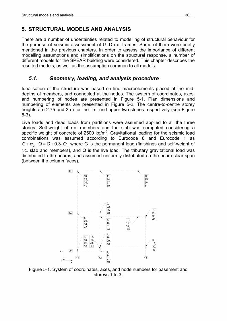
Structural models and analysis 36
5. STRUCTURAL MODELS AND ANALYSIS
There are a number of uncertainties related to modelling of structural behaviour for the purpose of seismic assessment of GLD r.c. frames. Some of them were briefly mentioned in the previous chapters. In order to assess the importance of different modelling assumptions and simplifications on the structural response, a number of different models for the SPEAR building were considered. This chapter describes the resulted models, as well as the assumption common to all models.
5.1. Geometry, loading, and analysis procedure
Idealisation of the structure was based on line macroelements placed at the mid-depths of members, and connected at the nodes. The system of coordinates, axes, and numbering of nodes are presented in Figure 5-1. Plan dimensions and numbering of elements are presented in Figure 5-2. The centre-to-centre storey heights are 2.75 and 3 m for the first und upper two stories respectively (see Figure 5-3). Live loads and dead loads from partitions were assumed applied to all the three stories. Self-weight of r.c. members and the slab was computed considering a specific weight of concrete of 2500 kg/m3. Gravitational loading for the seismic load combinations was assumed according to Eurocode 8 and Eurocode 1 as
2 0.3iG Q G Qψ+ ⋅ = + ⋅ , where G is the permanent load (finishings and self-weight of r.c. slab and members), and Q is the live load. The tributary gravitational load was distributed to the beams, and assumed uniformly distributed on the beam clear span (between the column faces).
X2
X1
X3
Y1 Y2 Y3
10, 23, 36, 49
8, 21, 34, 47
1, 13, 26, 39
2, 14, 27, 40
3, 15, 28, 41
4, 16, 29, 42
6, 18, 31, 44
9, 22, 35, 48
11, 24, 37, 50
5, 17, 30, 43
7, 20, 33, 46-,
19, 32, 45
12, 25, 38, 51
Z
Y
X Figure 5-1. System of coordinates, axes, and node numbers for basement and
storeys 1 to 3.

Structural models and analysis 37
3.00 6.00
5.00
5.50
0.50
4.00
6.00
3.00 5.00 1.70
B1, 15, 29
C5, 14, 23 C1, 10, 19 C2, 11, 20
C9, 18, 27
C3, 12, 21
C4, 13, 22
C7, 16, 25C6, 15, 24C8, 17, 26
B2, 16, 30
B3, 17, 31B4, 18, 32
B6, 20, 34B5, 19, 33
B11
, 25,
39
B12
, 26,
40
B9,
23,
37
B7,
21,
35
B8,
22,
36
B10
, 24,
38
B14, 28, 42
B13, 27, 41
0.70
1.00
10.5
0
9.70
X3
X2
X1
Y1 Y2 Y3Z
Y
X
Figure 5-2. Plan dimensions and element numbering for storeys 1 to 3 (dim. in m).
6.003.00
Y1 Y2 Y3
2.50
0.50
2.50
0.50
2.50
0.50
2.75
3.00
3.00
Z
X
Figure 5-3. Vertical cross-section through the structure (dimensions in m).
Rigid diaphragm action was considered at the floor levels, due to monolithic r.c. slab. Masses were determined according to the EC8 as corresponding to the loads from the 2iG Qϕ ψ+ ⋅ ⋅ combination, where ϕ=0.8 for stories 1-2 and 1.0 for roof. Translational masses (M) and mass moment of inertia (MMI) were applied at the centre of mass (CM) of each floor (see Table 5-1).

Structural models and analysis 38
Table 5-1. Translational masses and mass moment of inertia of the SPEAR building.
Centre of Mass Mass Mass Moment of Inertia
FLOOR 1&2 X = 4.53 m Y = 5.29 m 65.5 t 1254 tm2
ROOF X = 4.57 m Y = 5.33 m 64.1 t 1196 tm2
Centre of stiffness for each floor, determined according to EC8 as the centre of stiffness of column moment of inertia is presented in Figure 5-4. Torsional characteristics used for classification of building regularity in plan in EC8 are presented in Figure 5-2, where e0x, e0y are eccentricities measured along the X and Y axes respectively, rx, ry are torsional radii, and ls is the radius of gyration of a floor in plan. The following conditions need to be verified for each principal direction to consider the structure as regular in plan:
0 0.3x xe r≤ ⋅ , 0 0.3y ye r≤ ⋅ (5-1)
x sr l≥ , y sr l≥ (5-2)
Thus, the SPEAR structure is classified as irregular in plan according to EC8 provisions. Torsional eccentricities are larger in the Y direction.
Table 5-2. Torsional characteristics of the SPEAR building.
e0x, m e0y, m rx, m ry, m ls, m 0.3rx 0.3ry FLOOR 1&2 1.302 1.037 1.44 2.57 4.38 0.43 0.77
ROOF 1.338 1.081 1.44 2.57 4.32 0.43 0.77
5.29
4.53 4.57
5.33
CMCM
CS1.30
1.04
FLOORS 1&2
3.23
4.25
4.25
CS
3.23
1.34
1.08
ROOF
Z X
Y Y
Z X
Figure 5-4. Centre of mass and elastic centre of stiffness of the SPEAR building.
Seismic response of the SPEAR structure was evaluated by two analysis procedures: nonlinear dynamic (time-history) and nonlinear static (pushover). Computer code CANNY (Li, 2002) was used in both cases.
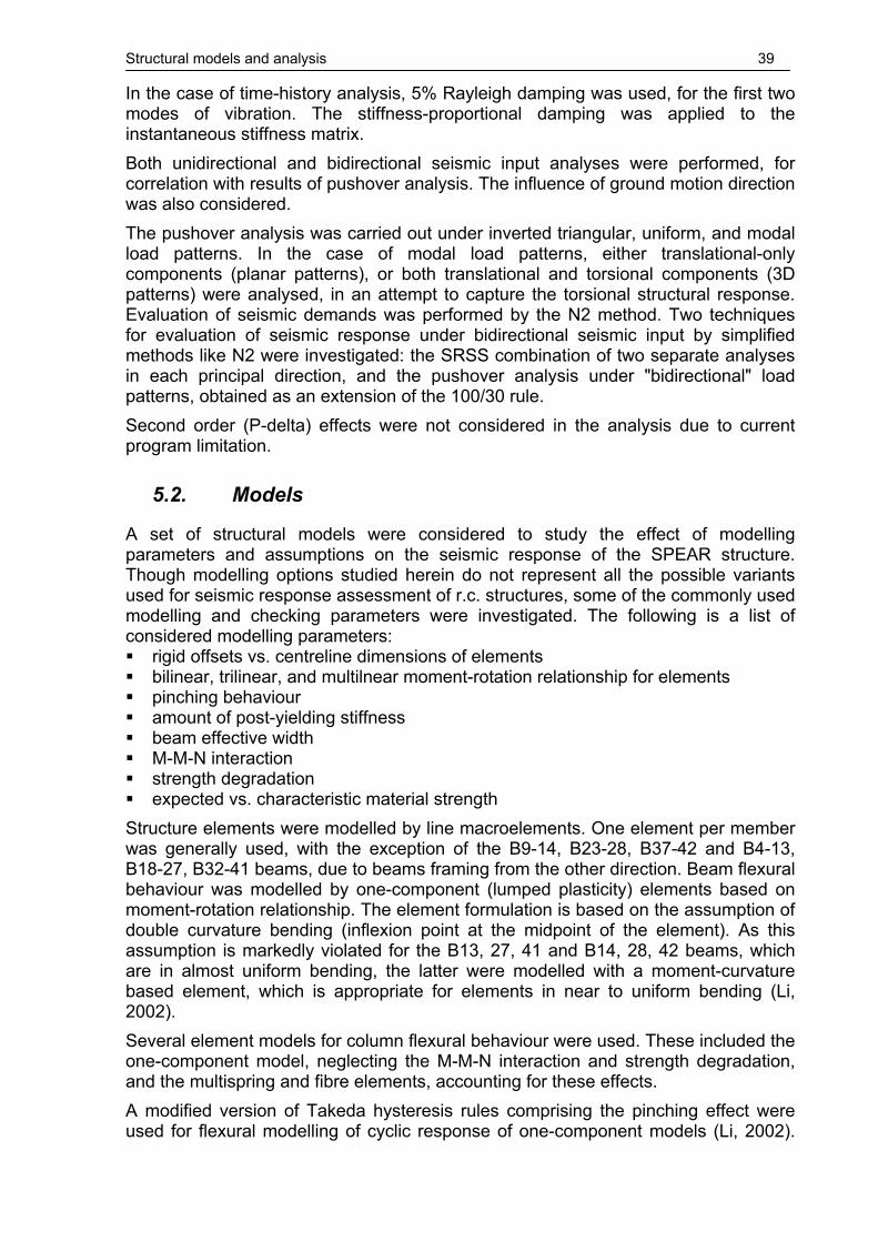
Structural models and analysis 39
In the case of time-history analysis, 5% Rayleigh damping was used, for the first two modes of vibration. The stiffness-proportional damping was applied to the instantaneous stiffness matrix. Both unidirectional and bidirectional seismic input analyses were performed, for correlation with results of pushover analysis. The influence of ground motion direction was also considered. The pushover analysis was carried out under inverted triangular, uniform, and modal load patterns. In the case of modal load patterns, either translational-only components (planar patterns), or both translational and torsional components (3D patterns) were analysed, in an attempt to capture the torsional structural response. Evaluation of seismic demands was performed by the N2 method. Two techniques for evaluation of seismic response under bidirectional seismic input by simplified methods like N2 were investigated: the SRSS combination of two separate analyses in each principal direction, and the pushover analysis under "bidirectional" load patterns, obtained as an extension of the 100/30 rule. Second order (P-delta) effects were not considered in the analysis due to current program limitation.
5.2. Models
A set of structural models were considered to study the effect of modelling parameters and assumptions on the seismic response of the SPEAR structure. Though modelling options studied herein do not represent all the possible variants used for seismic response assessment of r.c. structures, some of the commonly used modelling and checking parameters were investigated. The following is a list of considered modelling parameters: rigid offsets vs. centreline dimensions of elements bilinear, trilinear, and multilnear moment-rotation relationship for elements pinching behaviour amount of post-yielding stiffness beam effective width M-M-N interaction strength degradation expected vs. characteristic material strength
Structure elements were modelled by line macroelements. One element per member was generally used, with the exception of the B9-14, B23-28, B37-42 and B4-13, B18-27, B32-41 beams, due to beams framing from the other direction. Beam flexural behaviour was modelled by one-component (lumped plasticity) elements based on moment-rotation relationship. The element formulation is based on the assumption of double curvature bending (inflexion point at the midpoint of the element). As this assumption is markedly violated for the B13, 27, 41 and B14, 28, 42 beams, which are in almost uniform bending, the latter were modelled with a moment-curvature based element, which is appropriate for elements in near to uniform bending (Li, 2002). Several element models for column flexural behaviour were used. These included the one-component model, neglecting the M-M-N interaction and strength degradation, and the multispring and fibre elements, accounting for these effects. A modified version of Takeda hysteresis rules comprising the pinching effect were used for flexural modelling of cyclic response of one-component models (Li, 2002).
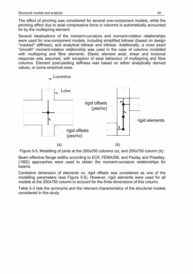
Structural models and analysis 40
The effect of pinching was considered for several one-component models, while the pinching effect due to axial compressive force in columns is automatically accounted for by the multispring element. Several idealisations of the moment-curvature and moment-rotation relationships were used for one-component models, including simplified bilinear (based on design "cracked" stiffness), and analytical bilinear and trilinear. Additionally, a more exact "smooth" moment-rotation relationship was used in the case of columns modelled with multispring and fibre elements. Elastic element axial, shear and torsional response was assumed, with exception of axial behaviour of multispring and fibre columns. Element post-yielding stiffness was based on either analytically derived values, or some empirical ones.
Lclear
Lcentreline
rigid offsets(yes/no)
rigid offsets(yes/no)
rigid elements
(a) (b)
Figure 5-5. Modelling of joints at the 250x250 columns (a), and 250x750 column (b). Beam effective flange widths according to EC8, FEMA356, and Paulay and Priestley, (1992) approaches were used to obtain the moment-curvature relationships for beams. Centreline dimension of elements vs. rigid offsets was considered as one of the modelling parameters (see Figure 5-5). However, rigid elements were used for all models at the 250x750 column to account for the finite dimensions of this column. Table 5-3 lists the acronyms and the relevant characteristics of the structural models considered in this study.

Structural models and analysis 41
Table 5-3. Structural models considered in this study.
Materials Element Beam eff. width Structure
DB design (D) one-component, bilinear EC8 rigid offsets
DBC design (D) one-component, bilinear EC8 centreline dimensions
DBCS design (D) one-component, bilinear code stiffness (0.5EcIg)
EC8 centreline dimensions
DT design (D) one-component, trilinear EC8 rigid offsets
DTC design (D) one-component, trilinear EC8 centreline dimensions
DT1H design (D) one-component, trilinear 1÷3% strain hardening EC8 rigid offsets
DT10H design (D) one-component, trilinear 10÷20% strain hardening EC8 rigid offsets
DTF design (D) one-component, trilinear FEMA356 rigid offsets
DTP design (D) one-component, trilinear moderate pinching for beams and columns
EC8 rigid offsets
DTP1 design (D) one-component, trilinear strong pinching for beams and columns
EC8 rigid offsets
DMS design (D) beams: trilinear columns: multispring EC8 rigid offsets
DMSa design (D)
beams: one-component, trilinear columns: multispring, "adjusted stiffness"
EC8 rigid offsets
DDMS design degrading (DD)
beams: one-component, trilinear columns: multispring
EC8 rigid offsets
EMS expected (E) beams: one-component, trilinear columns: multispring
EC8 rigid offsets
ETCP expected (E) one-component, trilinear (beams and columns)
Paulay and Priestley
centreline dimensions*
EFCP expected (E) beams: one-component, trilinear columns: fibre
Paulay and Priestley
centreline dimensions*
* centreline height of the first storey considered equal to 3 m, see discussion in chapter 8.2.
5.3. Dynamic characteristics
Initial periods of vibration vary considerably from one model to another (see Table 5-4) due to substantially different initial stiffness of different models. Though all mode shapes have components in all three degrees of freedom (two horizontal translations and torsional rotations), the predominant directions of vibration are X translations for the 1st mode, Y translations for the 2nd mode, and torsional rotations for the 3rd mode (see Figure 5-6).

Structural models and analysis 42
Table 5-4. The first three periods of vibration for the structural models considered.
Model T1, s T2, s T3, s DB 0.974 0.900 0.719 DBC 1.165 1.061 0.843 DBCS 0.776 0.667 0.535 DT, DT10H, DT1H, DTPB, DTP, DTP1 0.467 0.413 0.329 DTF 0.461 0.400 0.322 DTC 0.557 0.481 0.387 DDMS, DMS, DMSa 0.464 0.402 0.322 EMS 0.452 0.391 0.313 ETCP 0.570 0.484 0.392 EFCP 0.559 0.476 0.385
0
5
10
05
10
0
2
4
6
8
X
ETCP − Mode 1
Y
Z
0
5
10
05
10
0
2
4
6
8
X
ETCP − Mode 2
Y
Z
0
5
10
05
10
0
2
4
6
8
X
ETCP − Mode 3
Y
Z
Figure 5-6. The first three mode shapes for the ETCP model.

Influence of analysis procedure 43
6. INFLUENCE OF ANALYSIS PROCEDURE
6.1. Effect of seismic input direction
A structure should resist the seismic action from any direction. For structures with clearly defined principal axes, the seismic inputs applied in the directions of these axes are deemed to provide the relevant response quantities. If the maximum response of the structure is sought, it is possible to consider a number of analyses at different angles of incidence of the seismic input. This is schematically shown in Figure 6-1 for only four possible angles of incidence, along the principal axes of the building. The response quantities may be then determined as the maximum of the considered seismic inputs. Alternatively, the seismic inputs applied at different angles may be considered as distinct seismic events, so that the mean of these directions would be assumed as the relevant response quantities. Influence of these two approaches on the maximum displacements and twist in the centre of mass of the top floor are shown in Figure 6-2. There is approximately 30% difference between the maximum and mean values. A correlation could be observed between the diagonal directions of seismic input (0° - 180°, and 90° - 270°). A maximum positive displacement in the 0° would correspond to a maximum negative displacement in the 180° direction, in the case of translational displacements (TX and TY). This is not true for the torsional displacement (RZ), in which case the both maximum and negative response is observed either for the 0°-180°, or 90°-270° pair of seismic inputs. Note that for each diagonal pair of seismic inputs the ratio between the acceleration time histories is the same, while for the orthogonal pair this ratio is altered by a -1 factor. The translational response (at the centre of mass) in a given direction is dominated by the acceleration time history component in the same direction, and is relatively insensitive to the component in the perpendicular direction. The torsional response, however, is equally sensitive to both components, and is thus affected by ratio between the two time histories.
Z
Y
X
+ax
+ay
0° 90°
-ay
+ax
-ay
180°
-ax
-ax
270°
+ay
Figure 6-1. Four possible bidirectional seismic inputs.

Influence of analysis procedure 44
AL1 AL2 CA1 KA1 KA2 MO1 MO20
20
40
60
80
100
120
140
160
180
EARTHQUAKE
TO
P D
ISP
LA
CE
ME
NT
D−T
X−R
3, m
m
DBC − 0.2g − POSITIVE DEFORMATIONS
MAX. OF DIR.MEAN. OF DIR.DYN. MEAN(MAX)DYN. MEAN(MEAN)090180270
AL1 AL2 CA1 KA1 KA2 MO1 MO2−180
−160
−140
−120
−100
−80
−60
−40
−20
0
EARTHQUAKE
TO
P D
ISP
LA
CE
ME
NT
D−T
X−R
3, m
m
DBC − 0.2g − NEGATIVE DEFORMATIONS
MAX. OF DIR.MEAN. OF DIR.DYN. MEAN(MAX)DYN. MEAN(MEAN)090180270
AL1 AL2 CA1 KA1 KA2 MO1 MO20
50
100
150
EARTHQUAKE
TO
P D
ISP
LA
CE
ME
NT
D−T
Y−R
3, m
m
DBC − 0.2g − POSITIVE DEFORMATIONS
MAX. OF DIR.MEAN. OF DIR.DYN. MEAN(MAX)DYN. MEAN(MEAN)090180270
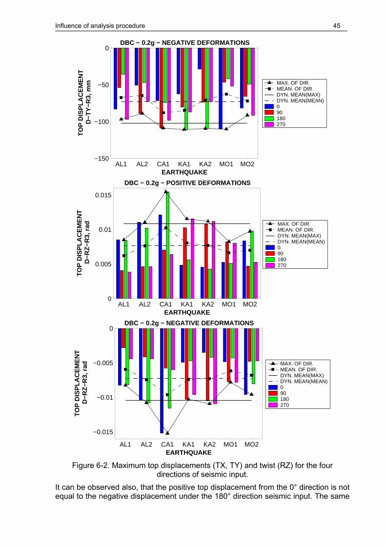
Influence of analysis procedure 45
AL1 AL2 CA1 KA1 KA2 MO1 MO2−150
−100
−50
0
EARTHQUAKE
TO
P D
ISP
LA
CE
ME
NT
D−T
Y−R
3, m
m
DBC − 0.2g − NEGATIVE DEFORMATIONS
MAX. OF DIR.MEAN. OF DIR.DYN. MEAN(MAX)DYN. MEAN(MEAN)090180270
AL1 AL2 CA1 KA1 KA2 MO1 MO20
0.005
0.01
0.015
EARTHQUAKE
TO
P D
ISP
LA
CE
ME
NT
D−R
Z−R
3, r
ad
DBC − 0.2g − POSITIVE DEFORMATIONS
MAX. OF DIR.MEAN. OF DIR.DYN. MEAN(MAX)DYN. MEAN(MEAN)090180270
AL1 AL2 CA1 KA1 KA2 MO1 MO2
−0.015
−0.01
−0.005
0
EARTHQUAKE
TO
P D
ISP
LA
CE
ME
NT
D−R
Z−R
3, r
ad
DBC − 0.2g − NEGATIVE DEFORMATIONS
MAX. OF DIR.MEAN. OF DIR.DYN. MEAN(MAX)DYN. MEAN(MEAN)090180270
Figure 6-2. Maximum top displacements (TX, TY) and twist (RZ) for the four
directions of seismic input. It can be observed also, that the positive top displacement from the 0° direction is not equal to the negative displacement under the 180° direction seismic input. The same

Influence of analysis procedure 46
is true for the 90°-270° combination. If the structure were symmetrical (stiffness and strength) with respect to its principal axes, the 0° direction positive displacement would have been equal to the 180° negative displacement, and vice versa. This particular structure is characterised by unequal strength in the positive and negative senses of a given direction (especially for the y direction), therefore there is some difference between the two senses. Considering the above observations, it may be concluded that the diagonally symmetric pairs of seismic input are not independent, and should be considered as representing the same seismic event. For unsymmetrical structures (with respect to strength) a distinction should be made between positive and negative response quantities, and the latter should be obtained as the maximum of the seismic input applied in the two senses (e.g. 0°-180°, or 90°-270°). Determination of the critical direction of seismic input by a series of time history analyses is not feasible due to the enormous amount of computational effort. Additionally, the question remains open whether the seismic inputs applied in different directions should be considered as representing the same event or different seismic events. Therefore it was decided for the rest of the study to retain only the 0°-180° pair of seismic inputs (see Figure 6-3a).
6.2. Effect of bidirectional seismic input
Consideration of the two horizontal ground motions components will depend on the analysis method involved. For time-history analysis the two components may be applied simultaneously (see Figure 6-3a), which is the straightforward way. Alternatively, two separate analysis may be performed in each direction (see Figure 6-3b), and the results combined according to one of the available rules. This is the standard procedure for linear elastic analysis and for the modal elastic analysis. The two combination rules widely used are: the square root of sum of squares (SRSS) method, 2 2
x yE E E= + the "100/30" rule, in which the relevant response quantities from 100% of the
seismic action applied in one direction are combined with the quantities from 30% of the seismic action applied in the perpendicular direction;
( )max 1.0 0.3 ; 0.3 1.0x y x yE E E E E= ⋅ + ⋅ ⋅ + ⋅
where Ex is the response quantity from the seismic action applied in the x direction, Ey is the response quantity from the seismic action applied in the y direction, and E is the prediction of the response quantity under bidirectional seismic input. Both methods were developed for elastic structural response, and are intended to recognize the fact that the two components of ground motion are statistically independent (i.e. the maximum response from the x direction will not occur at the same instant with the maximum response from the y direction). The SRSS method is more general, and does not depend on the chosen system of coordinates.

Influence of analysis procedure 47
0°
+ax
+ay
Z
Y
X
-ax
180°-ay
180° Y
+ay
0° X
Y
ZX
x
-ay
0° Y
180° X
(a) (b)
Figure 6-3. Two bidirectional (a) and the corresponding four one-directional (b) seismic inputs.
Influence of bidirectional seismic input and the validity of the SRSS combination rule in the inelastic range of response was studied by performing a set of unidirectional (see Figure 6-3b) and bidirectional (see Figure 6-3a) time history analyses for the DBC, DT, DMS, and DDMS models. One-component elements neglecting M-M-N interaction are used in the former two cases, and multispring elements accounting for M-M-N interaction are used in the latter two cases. A feature common for all cases is the amplification of torsional effects under bidirectional seismic input (see Figure 6-4 and Figure 6-5). The amplification is ground motion – dependent (lower or no torsional amplification is observed for the KA1 KA2 MO1 records for all models). The SRSS combination of unidirectional maxima seriously underestimates the bidirectional response. A better correlation may be observed in the case of direct addition of the unidirectional top storey twists (ABS). In the case of the DT model, very high amplifications of the top storey twists under bidirectional seismic input were observed, so that even the ABS combination of unidirectional results was unconservative. However, the torsional contribution is only a part of the total translational response. The latter showed to vary considerably with the model. Thus, for the DBC model, little amplification of top storey translations due to bidirectional input were observed at both the stiff and flexible edges (see Figure 6-6). A reduction of response was present in some cases (translation in the y direction at the flexible edge, see Figure 6-7). The SRSS combination rule provided good agreement, slightly conservative, with the exact bidirectional response. Note that the SRSS estimation of a response quantity will be always higher than the two unidirectional components, while there is a possibility for the bidirectional response to be lower than the governing unidirectional response (displacement in the direction of the seismic input). The direct addition of the unidirectional components constantly overestimated the results of the bidirectional analysis.

Influence of analysis procedure 48
AL1 AL2 CA1 KA1 KA2 MO1 MO20
0.005
0.01
0.015
EARTHQUAKE
TO
P D
ISP
LA
CE
ME
NT
D−R
Z−R
3, r
ad
DBC − 0.2g 1d − POSITIVE DEFORMATIONS
MAX. OF XMAX. OF YMAX. OF BIDIRMEAN OF XMEAN OF YMEAN OF BIDIRSRSSABS
Figure 6-4. Top storey twist for the DBC model.
AL1 AL2 CA1 KA1 KA2 MO1 MO20
1
2
3
4
5
6
7x 10
−3
EARTHQUAKE
TO
P D
ISP
LA
CE
ME
NT
D−R
Z−R
3, r
ad
DMS − 0.2g 1d − POS. DEF.
MAX. OF XMAX. OF YMAX. OF BIDIRMEAN OF XMEAN OF YMEAN OF BIDIRSRSSABS
Figure 6-5. Top storey twist for the DMS model.
AL1 AL2 CA1 KA1 KA2 MO1 MO20
50
100
150
EARTHQUAKE
TO
P D
ISP
LA
CE
ME
NT
D−T
X−N
39, m
m
DBC − 0.2g 1d − POSITIVE DEFORMATIONS
MAX. OF XMAX. OF YMAX. OF BIDIRMEAN OF XMEAN OF YMEAN OF BIDIRSRSSABS

Influence of analysis procedure 49
AL1 AL2 CA1 KA1 KA2 MO1 MO20
50
100
150
EARTHQUAKE
TO
P D
ISP
LA
CE
ME
NT
D−T
X−N
51, m
m
DBC − 0.2g 1d − POSITIVE DEFORMATIONS
MAX. OF XMAX. OF YMAX. OF BIDIRMEAN OF XMEAN OF YMEAN OF BIDIRSRSSABS
Figure 6-6. Influence of bidirectional input on top displacement in the X direction at
the stiff (N39) and flexible (N51) edges of the DBC model.
AL1 AL2 CA1 KA1 KA2 MO1 MO20
50
100
150
EARTHQUAKE
TO
P D
ISP
LA
CE
ME
NT
D−T
Y−N
39, m
m
DBC − 0.2g 1d − POSITIVE DEFORMATIONS
MAX. OF XMAX. OF YMAX. OF BIDIRMEAN OF XMEAN OF YMEAN OF BIDIRSRSSABS
AL1 AL2 CA1 KA1 KA2 MO1 MO20
50
100
150
EARTHQUAKE
TO
P D
ISP
LA
CE
ME
NT
D−T
Y−N
51, m
m
DBC − 0.2g 1d − POSITIVE DEFORMATIONS
MAX. OF XMAX. OF YMAX. OF BIDIRMEAN OF XMEAN OF YMEAN OF BIDIRSRSSABS
Figure 6-7. Influence of bidirectional input on top displacement in the Y direction at
the stiff (N39) and flexible (N51) edges of the DBC model.

Influence of analysis procedure 50
AL1 AL2 CA1 KA1 KA2 MO1 MO20
20
40
60
80
100
120
EARTHQUAKE
TO
P D
ISP
LA
CE
ME
NT
D−T
X−N
39, m
m
DT − 0.2g 1d − POSITIVE DEFORMATIONS
MAX. OF XMAX. OF YMAX. OF BIDIRMEAN OF XMEAN OF YMEAN OF BIDIRSRSSABS
AL1 AL2 CA1 KA1 KA2 MO1 MO20
20
40
60
80
100
120
EARTHQUAKE
TO
P D
ISP
LA
CE
ME
NT
D−T
X−N
51, m
m
DT − 0.2g 1d − POSITIVE DEFORMATIONS
MAX. OF XMAX. OF YMAX. OF BIDIRMEAN OF XMEAN OF YMEAN OF BIDIRSRSSABS
Figure 6-8. Influence of bidirectional input on top displacement in the X direction at
the stiff (N39) and flexible (N51) edges of the DT model. In the case of the DT model (see Figure 6-8) the average top displacement at the stiff edge under bidirectional excitation was smaller than the governing displacement under unidirectional seismic input. An opposite trend was observed at the flexible edge. Due to small torsional response under unidirectional ground motions, the SRSS combination was very close to the governing unidirectional response. Also, there was less difference between the direct addition and SRSS combination of results. However, both combination techniques either overestimated or underestimated the bidirectional response.

Influence of analysis procedure 51
AL1 AL2 CA1 KA1 KA2 MO1 MO20
20
40
60
80
100
EARTHQUAKE
TO
P D
ISP
LA
CE
ME
NT
D−T
X−N
39, m
m
DMS − 0.2g 1d − POSITIVE DEFORMATIONS
MAX. OF XMAX. OF YMAX. OF BIDIRMEAN OF XMEAN OF YMEAN OF BIDIRSRSSABS
AL1 AL2 CA1 KA1 KA2 MO1 MO20
20
40
60
80
100
EARTHQUAKE
TO
P D
ISP
LA
CE
ME
NT
D−T
X−N
51, m
m
DMS − 0.2g 1d − POSITIVE DEFORMATIONS
MAX. OF XMAX. OF YMAX. OF BIDIRMEAN OF XMEAN OF YMEAN OF BIDIRSRSSABS
Figure 6-9. Influence of bidirectional input on top displacement in the X direction at
the stiff (N39) and flexible (N51) edges of the DMS model. Both DMS and DDMS models (accounting for M-M-N interaction) showed the same trend of higher top displacements under bidirectional excitation than the governing displacement under unidirectional excitation at both flexible and stiff edges (see Figure 6-9). The SRSS combination of unidirectional response quantities was close to the governing unidirectional response, and failed to predict the bidirectional response. The influence of torsional response under unidirectional and bidirectional seismic input on top displacements' time-history is shown in Figure 6-10 and Figure 6-11, for the DBC and DMS models respectively. It can be observed that under unidirectional seismic input top displacements in the direction of the excitation at the flexible and stiff edges, as well as top twist are in phase. Though local maxima are attained at approximately the same time instances for both displacements and twist, maximum twists generally do not occur simultaneously with maximum translations. Top edge displacements in the direction perpendicular to the seismic input are generally also in phase with top twist. However, some phase difference was observed for some records, especially after the main peak. Also, the displacements at the flexible edge are not necessarily greater than those at the stiff edge. Under unidirectional excitation the average displacements perpendicular to the seismic input are of the

Influence of analysis procedure 52
order of 10% and 25% of the displacements in the direction of seismic input, at the centre of mass and edges, respectively.
2 4 6 8 10 12 14 16 18 20 22−200
−100
0
100
200
TIME, s
DIS
PL
AC
EM
EN
T, m
m
DBC − 0.2g 1d − TOP DISPLACEMENT TH, AL1−0 X
D−TX−N39 D−TX−N51
2 4 6 8 10 12 14 16 18 20 22−5
0
5
RO
TA
TIO
N, m
rad
D−RZ−R3
2 4 6 8 10 12 14 16 18 20 22−50
0
50
TIME, s
DIS
PL
AC
EM
EN
T, m
m
DBC − 0.2g 1d − TOP DISPLACEMENT TH, AL1−0 Y
D−TX−N39 D−TX−N51
2 4 6 8 10 12 14 16 18 20 22−5
0
5
RO
TA
TIO
N, m
rad
D−RZ−R3
0 2 4 6 8 10 12 14 16 18 20 22−200
−100
0
100
200
TIME, s
DIS
PL
AC
EM
EN
T, m
m
DBC − 0.2g − TOP DISPLACEMENT TH, AL1−0
D−TX−N39 D−TX−N51
0 2 4 6 8 10 12 14 16 18 20 22−10
−5
0
5
10
RO
TA
TIO
N, m
rad
D−RZ−R3
Figure 6-10. Time history of top displacements at the stiff (TX-N39) and flexible (TX-N51) edges, and the top twist (RZ-R3) for the DBC model.
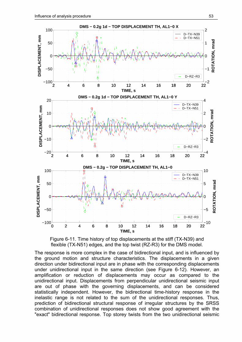
Influence of analysis procedure 53
2 4 6 8 10 12 14 16 18 20 22−100
−50
0
50
100
TIME, s
DIS
PL
AC
EM
EN
T, m
m
DMS − 0.2g 1d − TOP DISPLACEMENT TH, AL1−0 X
D−TX−N39 D−TX−N51
2 4 6 8 10 12 14 16 18 20 22−2
−1
0
1
2
RO
TA
TIO
N, m
rad
D−RZ−R3
2 4 6 8 10 12 14 16 18 20 22−20
−10
0
10
20
TIME, s
DIS
PL
AC
EM
EN
T, m
m
DMS − 0.2g 1d − TOP DISPLACEMENT TH, AL1−0 Y
D−TX−N39 D−TX−N51
2 4 6 8 10 12 14 16 18 20 22−4
−2
0
2
4
RO
TA
TIO
N, m
rad
D−RZ−R3
0 2 4 6 8 10 12 14 16 18 20 22−100
−50
0
50
100
TIME, s
DIS
PL
AC
EM
EN
T, m
m
DMS − 0.2g − TOP DISPLACEMENT TH, AL1−0
D−TX−N39 D−TX−N51
0 2 4 6 8 10 12 14 16 18 20 22−10
−5
0
5
10
RO
TA
TIO
N, m
rad
D−RZ−R3
Figure 6-11. Time history of top displacements at the stiff (TX-N39) and flexible (TX-N51) edges, and the top twist (RZ-R3) for the DMS model.
The response is more complex in the case of bidirectional input, and is influenced by the ground motion and structure characteristics. The displacements in a given direction under bidirectional input are in phase with the corresponding displacements under unidirectional input in the same direction (see Figure 6-12). However, an amplification or reduction of displacements may occur as compared to the unidirectional input. Displacements from perpendicular unidirectional seismic input are out of phase with the governing displacements, and can be considered statistically independent. However, the bidirectional time-history response in the inelastic range is not related to the sum of the unidirectional responses. Thus, prediction of bidirectional structural response of irregular structures by the SRSS combination of unidirectional responses does not show good agreement with the "exact" bidirectional response. Top storey twists from the two unidirectional seismic

Influence of analysis procedure 54
inputs are also out of phase (see Figure 6-13). However, an important amplification of top twist under bidirectional seismic input was noted for all models. While under unidirectional seismic input only the resisting plane in the direction of input yields, under bidirectional input both planes yield, leading to a reduction of torsional resistance and increase in torsional displacements.
10 20−100
−50
0
50
100
150
TIME, s
DIS
PL
AC
EM
EN
T, m
m
DBC − 0.2g 1d − TOP DISPLACEMENT TH, D−TX−N51
AL1−0 XAL1−0 YAL1−0
10 20−50
0
50
100
TIME, s
DIS
PL
AC
EM
EN
T, m
m
DMS − 0.2g 1d − TOP DISPLACEMENT TH, D−TX−N51
AL1−0 XAL1−0 YAL1−0
Figure 6-12. Time history of top displacement at the flexible (TX-N51) edge under
unidirectional and bidirectional excitation. Due to weak columns, the effects of bidirectional seismic input are amplified in the case of models accounting for M-M-N interaction (DMS, DDMS). The bidirectional seismic input will reduce the strength and stiffness of columns subjected to bidirectional moments and varying axial force (see Figure 6-14b). One-component models (see Figure 6-14a) fail to represent this phenomena. Thus, displacements at the centre of mass under bidirectional seismic input show little difference to the ones from the governing unidirectional input. For the DMS and DDMS models, the bidirectional response is related not only to the influence of torsion, but also to the degradation of stiffness and strength, therefore increased displacements demands are observed not only at the edges, but also at the centre of mass.

Influence of analysis procedure 55
10 20−10
−5
0
5
10
TIME, s
RO
TA
TIO
N, m
rad
DBC − 0.2g 1d − TOP DISPLACEMENT TH, D−RZ−R3
AL1−0 XAL1−0 YAL1−0
10 20−10
−5
0
5
TIME, s
RO
TA
TIO
N, m
rad
DMS − 0.2g 1d − TOP DISPLACEMENT TH, D−RZ−R3
AL1−0 XAL1−0 YAL1−0
Figure 6-13. Time history of top twist under unidirectional and bidirectional excitation.
−5 0 5
x 10−3
−40
−20
0
20
40
Mx1 − ROTATION, rad
MO
ME
NT
, kN
m
DT − 0.2g 1d − C2
AL2−0 XAL2−0 YAL2−0
−5 0 5
x 10−3
−40
−20
0
20
40
Mx1 − ROTATION, rad
MO
ME
NT
, kN
m
DMS − 0.2g 1d − C2
AL2−0 XAL2−0 YAL2−0
(a) (b)
Figure 6-14. Reduction of column strength due to bidirectional seismic input. No trends have been observed that would make possible derivation of the bidirectional response from two independent unidirectional responses, with exception of torsional response (top storey twist), where direct addition of the two unidirectional maxima provided close agreement with the bidirectional response. Top displacements in a given direction from unidirectional excitation are higher at the flexible edge. The effect of bidirectional input is to increase or decrease the displacements due to unidirectional response, results being dependent on the structural model and particular earthquake record. However, the translational

Influence of analysis procedure 56
response in a given direction from bidirectional input is dictated by the corresponding response under unidirectional input. If structural elements prone to the M-M-N interaction represent the weak link in the structural system, bidirectional input leads to a reduction of resistance and increase of displacements if the M-M-N effects are accounted for.
6.3. Pushover analysis
If a 3D structural model is employed, bidirectional input is the straightforward way for a dynamic non-linear analysis. When simplified methods based on pushover analysis are used for evaluation of structural response of a 3D irregular structure, no clear rules are available. The two main problems are related to the selection of an appropriate load pattern that would reliably predict the unidirectional response, and the consideration of the bidirectional seismic input. The N2 method (Fajfar, 2000) for simplified evaluation of the seismic demand was used in this study. It involves a static nonlinear (pushover) analysis of the MDOF structure combined with a response spectrum analysis of an equivalent SDOF system. The method was initially restricted to planar structures. The theoretical background of its extension to asymmetric 3D structures is presented in Fajfar, 2002.
6.3.1. Load patterns
For planar structural models, the load patterns largely used for pushover analysis are the inverted triangular, uniform, and modal. The deflection shape of the fundamental mode of vibration is close the inverted triangular load pattern for low-rise structures with uniform vertical distribution of mass and stiffness, therefore they are expected to provide similar results in these cases. In the N2 method the load patterns are related to the displacement shapes. The load shape (pattern) is determined from the assumed displacement shape weighted by the storey masses. In the case of 3D structural model, the displacement shape may contain only the displacement components in the direction of the pushover analysis, or contain as well translational components in the orthogonal direction and /or torsional components. In an attempt to predict the torsional response under unidirectional seismic input by a pushover analysis, several displacement shapes were considered. Two of them are the "classic" inverted triangular (TRIANG) and uniform (UNIF) displacement shapes, containing translational components in one direction only. The third one (MODE1) was obtained by the translational components of the modal shape with predominant vibration in the direction considered, i.e. first and second mode of vibration for the displacement shapes in the X and Y direction respectively. The first two modal shapes of the structure are predominantly translational, with the dominating translations in the X direction for the first, and Y direction for the second mode. The third mode is predominantly torsional. Two more load patterns for each direction were formed based on the dominant modal translations. "MODE1 FULL" displacement shape was formed by the modal displacements (translations and twists) of the first mode for the X direction and the second mode for the Y direction. "MODE1 TRS" was formed in a similar way, but only the dominant translations (in the X or Y direction) and twists were considered, i.e. translational components orthogonal to the dominant translations were omitted. Load patterns were applied in the centre of mass of each floor. The first three periods of vibration for the models considered are presented in Table 5-4, while the load patterns for some of the models are presented in Table 6-1 through Table 6-4.

Influence of analysis procedure 57
Table 6-1. Load patterns for the DB model.
Pattern TRIANG UNIF MODE1 MODE1 FULL
MODE1 TRS
Direction X Y X Y X Y X Y X Y Fx
3, kN 64.1 - 64.1 - 64.1 - 64.1 20.0 64.1 - Fx
2, kN 43.0 - 65.5 - 48.9 - 48.9 15.5 48.9 - Fx
1, kN 20.6 - 65.5 - 23.3 - 23.3 7.31 23.3 - Fy
3, kN - 64.1 - 64.1 - 64.1 -17.7 64.1 - 64.1 Fy
2, kN - 43.0 - 65.5 - 46.0 -12.7 46.0 - 46.0 Fy
1, kN - 20.6 - 65.5 - 19.0 -5.4 19.0 - 19.0 Mz
3, kNm - - - - - - -53.3 74.8 -53.3 74.8 Mz
2, kNm - - - - - - -42.3 60.6 -42.3 60.6 Mz
1, kNm - - - - - - -21.4 30.7 -21.4 30.7
Note: Fij represents the force or moment applied in the direction i at the storey j.
Table 6-2. Load patterns for the DBC model.
Pattern TRIANG UNIF MODE1 MODE1 FULL
MODE1 TRS
Direction X Y X Y X Y X Y X Y Fx
3, kN 64.1 - 64.1 - 64.1 - 64.1 16.5 64.1 - Fx
2, kN 43.0 - 65.5 - 47.3 - 47.3 12.5 47.3 - Fx
1, kN 20.6 - 65.5 - 20.0 - 20.0 5.2 20.0 - Fy
3, kN - 64.1 - 64.1 - 64.1 -13.6 64.1 - 64.1 Fy
2, kN - 43.0 - 65.5 - 44.6 -9.5 44.6 - 44.6 Fy
1, kN - 20.6 - 65.5 - 16.7 -3.7 16.7 - 16.7 Mz
3, kNm - - - - - - -50.2 86.4 -50.2 86.4 Mz
2, kNm - - - - - - -38.4 67.8 -38.4 67.8 Mz
1, kNm - - - - - - -17.1 30.6 -17.1 30.6
Table 6-3. Load patterns for the DT model.
Pattern TRIANG UNIF MODE1 MODE1 FULL
MODE1 TRS
Direction X Y X Y X Y X Y X Y Fx
3, kN 64.1 - 64.1 - 64.1 - 64.1 30.5 64.1 - Fx
2, kN 43.0 - 65.5 - 50.9 - 50.9 24.4 50.9 - Fx
1, kN 20.6 - 65.5 - 26.2 - 26.2 12.4 26.2 - Fy
3, kN - 64.1 - 64.1 - 64.1 -24.4 64.1 - 64.1 Fy
2, kN - 43.0 - 65.5 - 47.5 -18.4 47.5 - 47.5 Fy
1, kN - 20.6 - 65.5 - 20.8 -8.5 20.8 - 20.8 Mz
3, kNm - - - - - - -105 87.0 -105 87.0 Mz
2, kNm - - - - - - -87.1 72.5 -87.1 72.5 Mz
1, kNm - - - - - - -46.0 38.3 -46.0 38.3

Influence of analysis procedure 58
Table 6-4. Load patterns for the DMS model.
Pattern TRIANG UNIF MODE1 MODE1 FULL
MODE1 TRS
Direction X Y X Y X Y X Y X Y Fx
3, kN 64.1 - 64.1 - 64.1 - 64.1 31.5 64.1 - Fx
2, kN 43.0 - 65.5 - 50.7 - 50.7 24.8 50.7 - Fx
1, kN 20.6 - 65.5 - 25.6 - 25.6 11.8 25.6 - Fy
3, kN - 64.1 - 64.1 - 64.1 -24.7 64.1 - 64.1 Fy
2, kN - 43.0 - 65.5 - 46.7 -18.5 46.7 - 46.7 Fy
1, kN - 20.6 - 65.5 - 19.1 -8.4 19.1 - 19.1 Mz
3, kNm - - - - - - -115 85.5 -115 85.5 Mz
2, kNm - - - - - - -96.1 70.3 -96.1 70.3 Mz
1, kNm - - - - - - -52.0 35.2 -52.0 35.2
Separate pushover analyses were performed in the positive and negative senses of each principal direction. Thus, "TRIANG 100X-P" stand for a pushover analysis performed under the inverted triangular load pattern, applied in the positive X direction. "Bidirectional" load patterns were investigated as well, as will be discussed later. They were formed by 100% of the load pattern applied in the relevant direction and 30% of the load pattern applied in the perpendicular direction. Thus, the load pattern "100X-P 30Y-N" is formed by 100% of the unidirectional load pattern applied in the positive X direction and 30% of the load applied in the negative Y direction. A comparison of the three single component load patterns (TRIANG, UNIF, and MODE1) is presented in Figure 6-15. There is little difference between the inverted triangular and modal load patterns, both in the shape of the pushover curve, and the characteristic events (first yield, attainment of ultimate rotation in elements, and displacement demand estimated by the N2 method). Attainment of the ultimate rotation capacity in the critical element is denoted in figures by DCR=1, the former standing for Demand to Capacity Ratio. The uniform load pattern imposes higher demands in the lower storey, promoting a first storey plastic mechanism. Its effect is prediction of increased stiffness and strength of the global pushover curve, and reduction of the displacement demands. A reduction of the global ductility predicted by the UNIF load pattern may also be noted, due to increase strength at first yield and reduced top displacement at the attainment of the rotation capacity in the critical elements (first storey columns). A comparison of the modal load patterns (MODE1, MODE1 FULL, and MODE1 TRS) is shown in Figure 6-16. Earlier first yield may be noted in the case of load patterns containing orthogonal translational and torsional components (MODE1 FULL, and MODE1 TRS), due to increased demands at the edge frames. A slight reduction of stiffness after first yield is present for the 3D load patterns in comparison with the planar load pattern for the case of the one-component models (DBC, DT). For models accounting for M-M-N interaction this decrease is more evident, and is accompanied by a reduction in strength, as well as earlier attainment of ultimate rotation in elements. The 3D load patterns impose a biaxial demand on the columns, reducing their strength. The MODE1 FULL load pattern is the most unfavourable, as it contains both orthogonal translational and torsional components. The effect of biaxial column demand is most evident when the degradation of column strength is considered in the DDMS model (see Figure 6-17). Top storey displacement demand

Influence of analysis procedure 59
by the N2 method decreases when the displacement shape contains torsional and/or orthogonal translational components. This is caused by the reduction of the coefficient Γ used to transform the MDOF system to the SDOF system and vice versa.
−200 −150 −100 −50 0 50 100 150 2000
50
100
150
200
250
300
350
TOP DISPLACEMENT, mm
BA
SE
SH
EA
R, k
N
DT − 0.2g
TRIANG−100XMODE1−100XUNIF−100X1st yieldDCR=1N2 DEMAND
−200 −150 −100 −50 0 50 100 150 2000
50
100
150
200
250
300
350
TOP DISPLACEMENT, mm
BA
SE
SH
EA
R, k
N
DMS − 0.2g
TRIANG−100XMODE1−100XUNIF−100X1st yieldDCR=1N2 DEMAND
Figure 6-15. Pushover curves in the X direction for load patterns with components in
a singe direction (DT and DMS models).

Influence of analysis procedure 60
−200 −150 −100 −50 0 50 100 150 2000
50
100
150
200
250
300
350
TOP DISPLACEMENT, mm
BA
SE
SH
EA
R, k
N
DT − 0.2g
MODE1−100XMODE1 FULL−100XMODE1 TRS−100X1st yieldDCR=1N2 DEMAND
−200 −150 −100 −50 0 50 100 150 2000
50
100
150
200
250
300
350
TOP DISPLACEMENT, mm
BA
SE
SH
EA
R, k
N
DMS − 0.2g
MODE1−100XMODE1 FULL−100XMODE1 TRS−100X1st yieldDCR=1N2 DEMAND
Figure 6-16. Pushover curves in the X direction for modal load patterns (DT and DMS
models).

Influence of analysis procedure 61
−200 −150 −100 −50 0 50 100 150 2000
50
100
150
200
250
300
350
TOP DISPLACEMENT, mm
BA
SE
SH
EA
R, k
N
DDMS − 0.2g
MODE1−100XMODE1 FULL−100XMODE1 TRS−100X1st yieldN2 DEMAND
Figure 6-17. Pushover curves in the X direction for modal load patterns (DDMS
model). Conservative predictions of the top displacement at the centre of mass in the direction of seismic input for unidirectional loading were obtained generally by the N2 method (see Figure 6-18). Single component load patterns (TRIANG, MODE1) provided higher demands than the 3D load patterns (MODE1 FULL, MODE1 TRS). Translations orthogonal to the direction of seismic input, as well as twists obtained from the pushover analysis were much scattered depending of the structural model (see Figure 6-19). A good agreement with the dynamic analysis was observed in case of the DBC mode, and a poor one for the DT, DMS, and DDMS models. It can be observed that the ratio of torsional and orthogonal translational load components to the translational components in the direction of the seismic input is changed by up to 100% from the DBC to the DT, DMS, and DDMS models. The shape of the load patterns is dictated by the modal shapes, which is sensitive to the modelling of initial stiffness of elements. DBC model uses the secant stiffness to the yield point for moment-rotation relationships of the elements (see Figure 4-4), while the other three models are based on uncracked initial stiffness of the gross cross-sections (trilinear and multispring modelling). The best agreement of torsional response (twists and translations at the edges) prediction by the pushover analysis with the dynamic analysis was observed for the DBC model and the MODE1 TRS load pattern (see Figure 6-20). However, on the expense of conservative predictions, especially at the stiff edge, the MODE1 and TRIANG load patterns were the most reliable, especially for the models based on initial uncracked stiffness (see Figure 6-20 and Figure 6-21). The main disadvantage of single component load patterns (MODE1 and TRIANG) is their underestimation of torsional response, displacements at the flexible edge having a lower safety margin than the ones at the stiff edge.

Influence of analysis procedure 62
X Y−150
−100
−50
0
50
100
150
DIRECTION OF SEISMIC INPUT
TO
P D
ISP
LA
CE
ME
NT
D−T
X−R
3, m
m
DBC − 0.2g 1d
MEAN DYN.MEAN DYN.+STDN2−MODE1N2−MODE1 FULLN2−MODE1 TRS
X Y−80
−60
−40
−20
0
20
40
60
80
DIRECTION OF SEISMIC INPUT
TO
P D
ISP
LA
CE
ME
NT
D−T
X−R
3, m
m
DMS − 0.2g 1d
MEAN DYN.MEAN DYN.+STDN2−MODE1N2−MODE1 FULLN2−MODE1 TRS
Figure 6-18. Mean dynamic vs. N2 prediction of top displacement at the centre of
mass for unidirectional seismic input (DBC and DMS models).
X Y−6
−4
−2
0
2
4
6x 10
−3
DIRECTION OF SEISMIC INPUT
TO
P D
ISP
LA
CE
ME
NT
D−R
Z−R
3, r
ad
DBC − 0.2g 1d
MEAN DYN.MEAN DYN.+STDN2−MODE1N2−MODE1 FULLN2−MODE1 TRS

Influence of analysis procedure 63
X Y−8
−6
−4
−2
0
2
4
6
8x 10
−3
DIRECTION OF SEISMIC INPUT
TO
P D
ISP
LA
CE
ME
NT
D−R
Z−R
3, r
ad
DMS − 0.2g 1d
MEAN DYN.MEAN DYN.+STDN2−MODE1N2−MODE1 FULLN2−MODE1 TRS
Figure 6-19. Mean dynamic vs. N2 prediction of top twists for unidir. seismic input.
X Y−150
−100
−50
0
50
100
150
DIRECTION OF SEISMIC INPUT
TO
P D
ISP
LA
CE
ME
NT
D−T
X−N
39, m
m
DBC − 0.2g 1d
MEAN DYN.MEAN DYN.+STDN2−MODE1N2−MODE1 FULLN2−MODE1 TRS
X Y−150
−100
−50
0
50
100
150
DIRECTION OF SEISMIC INPUT
TO
P D
ISP
LA
CE
ME
NT
D−T
X−N
51, m
m
DBC − 0.2g 1d
MEAN DYN.MEAN DYN.+STDN2−MODE1N2−MODE1 FULLN2−MODE1 TRS
Figure 6-20. Mean dynamic vs. N2 prediction of top displacement at the stiff (N39)
and flexible (N51) edges for unidirectional seismic input (DBC model).

Influence of analysis procedure 64
X Y−80
−60
−40
−20
0
20
40
60
80
DIRECTION OF SEISMIC INPUT
TO
P D
ISP
LA
CE
ME
NT
D−T
X−N
39, m
m
DMS − 0.2g 1d
MEAN DYN.MEAN DYN.+STDN2−MODE1N2−MODE1 FULLN2−MODE1 TRS
X Y−100
−50
0
50
100
DIRECTION OF SEISMIC INPUT
TO
P D
ISP
LA
CE
ME
NT
D−T
X−N
51, m
m
DMS − 0.2g 1d
MEAN DYN.MEAN DYN.+STDN2−MODE1N2−MODE1 FULLN2−MODE1 TRS
Figure 6-21. Mean dynamic vs. N2 prediction of top displacement at the stiff (N39)
and flexible (N51) edges for unidirectional seismic input (DMS model). Selection of an appropriate load pattern is a critical factor for the pushover analysis. Though 3D load patterns containing orthogonal displacements to the direction of the seismic input and/or torsional components may provide a better correlation between the pushover and time-history analysis, it is difficult to select such a pattern. Load patterns derived from the first two mode shapes are sensitive to modelling of the initial stiffness of elements, and showed to be inadequate when based on the initial uncracked stiffness. Correlation between the top translation in the direction of the seismic input and perpendicular to it in the case of pushover and dynamic analyses is shown in Figure 6-22 and Figure 6-23. It can be observed a gross disagreement between the MODE1 FULL pushover in the Y direction based on the second mode of vibration, and the unidirectional dynamic response. Inclusion of only torsional components beside the translations in the direction of seismic input (MODE1 TRS) seems to be a better option for 3D pushover analysis. However, it is not appropriate to be based on the initial uncracked stiffness modelling.

Influence of analysis procedure 65
−300 −200 −100 0 100 200 300−60
−40
−20
0
20
40
60
TX, mm
TY
, mm
DMS − 0.2g
MODE1−100XMODE1 FULL−100XMODE1 TRS−100X1st yieldDCR=1N2 DEMAND
−100 −50 0 50 100−300
−200
−100
0
100
200
300
TX, mm
TY
, mm
DMS − 0.2g
MODE1−100YMODE1 FULL−100YMODE1 TRS−100Y1st yieldDCR=1N2 DEMAND
Figure 6-22. Top displacements at the centre of mass in the direction and
perpendicular to the seismic input (pushover analysis, DMS model).

Influence of analysis procedure 66
−50 0 50−80
−60
−40
−20
0
20
40
60
80
D−TX−R3, mm
D−T
Y−R
3, m
mDMS − 0.2g 1d, TOP DISP.
AL1−0 XAL1−0 YAL1−0
−50 0 50
−60
−40
−20
0
20
40
60
D−TX−R3, mm
D−T
Y−R
3, m
m
DMS − 0.2g 1d, TOP DISP.
AL2−0 XAL2−0 YAL2−0
Figure 6-23. Top displacements at the centre of mass in the direction and
perpendicular to the seismic input (dynamic analysis, DMS model, AL1 and AL2 ground motion records applied in the 0° direction).
6.3.2. Influence of strength asymmetry
Pushover curves in the positive and negative X and Y directions are presented in Figure 6-24. It can be observed an asymmetry in strength for the positive and negative senses of the Y direction of loading.
0 20 40 60 80 100 120 140 160 180 2000
50
100
150
200
250
300
350
TOP DISPLACEMENT, mm
BA
SE
SH
EA
R, k
N
DMS − 0.2g − TRIANG
100X−P100X−N100Y−P100Y−N1st yieldDCR=1N2 DEMAND
Figure 6-24. Pushover curves in the positive and negative X/Y directions, TRIANG
load pattern, DMS model.

Influence of analysis procedure 67
X Y−100
−50
0
50
100
DIRECTION OF SEISMIC INPUT
TO
P D
ISP
LA
CE
ME
NT
D−T
Y−R
3, m
m
DT − 0.2g 1d
MEAN DYN.MEAN DYN.+STDN2−MODE1N2−MODE1 FULLN2−MODE1 TRS
X Y−100
−50
0
50
100
DIRECTION OF SEISMIC INPUT
TO
P D
ISP
LA
CE
ME
NT
D−T
Y−R
3, m
m
DMS − 0.2g 1d
MEAN DYN.MEAN DYN.+STDN2−MODE1N2−MODE1 FULLN2−MODE1 TRS
Figure 6-25. Positive vs. negative displacements at the centre of mass in the Y
direction, DT and DMS models. Higher displacement demands are predicted by dynamic analysis in the positive as compared to negative senses of the Y direction, due to the lower strength in the former case. The simplified pushover/N2 method fails to predict this behaviour, though lower global strength affects the bilinear idealisation of the capacity curve in the simplified analysis method, leading to a slight increase of displacement demands. However, this effect is minor when compared to the difference between positive and negative displacement estimates of the dynamic analysis. A comparison of dynamic and pushover predictions of top displacement in the positive and negative senses of the Y direction is presented in Figure 6-25. Though in the case of DMS and DDMS models the simplified method provided conservative estimates for both positive and negative senses (MODE1 load pattern), overpredicting displacement demands in the stronger (negative) sense, it was slightly unconservative in the case of positive displacement demands of the DBC and DT models. Thus, caution is necessary in applying simplified methods based on pushover analysis to structures with strong strength asymmetry.

Influence of analysis procedure 68
6.3.3. Bidirectional seismic input
In the case of static inelastic (pushover) structural analysis the superposition of response quantities from two separate analyses in each principal direction is not correct. Though it lacks theoretical background, the SRSS rule was used for combination of directional effects by pushover analysis (Fajfar et al., 2000). Another possibility, which deserves additional investigation, is the pushover analysis under bidirectional load input. A "bidirectional" load input is formed by applying 100% of the load pattern in one direction simultaneously with 30% of the load pattern in the perpendicular direction. This eliminates the need for superposition of results from separate unidirectional analyses in the two directions. However, it requires more analysis runs, as several 100/30 combinations are possible. Alternatively, most unfavourable ones (increasing torsional response) may be chosen based on engineering judgement. A comparison of unidirectional vs. bidirectional pushover analyses are presented in Figure 6-26 and Figure 6-27 for the DBC and DMS models, respectively. In the case of single component load patterns (MODE1), there is little influence of the bidirectional load pattern. Depending on the 100/30 combination, later or earlier yielding of the first element is observed. For example, earlier yielding is observed for the "100X-N 30Y-N" load pattern and later for the "100X-N 30Y-P" as compared to the unidirectional "100X-N", as the torsional effects from the orthogonal loading (30Y) act in the same or opposite sense with the torsional effects of the principal loading (100X-N), respectively. The effect of bidirectional load patterns increases for MODE1 TRS load patterns, as the combined torsional effect from each pattern (100 and 30) increases. The reduction or increase in strength and stiffness due to the 100/30 load patterns is most evident in the case DMS model, accounting for M-M-N interaction and is reduced for one-component based DBC model.
−200 −150 −100 −50 0 50 100 150 2000
50
100
150
200
250
300
350
TOP DISPLACEMENT, mm
BA
SE
SH
EA
R, k
N
DBC − 0.2g − MODE1
100X−P100X−N100X−P 30Y−P100X−P 30Y−N100X−N 30Y−P100X−N 30Y−N1st yieldDCR=1N2 DEMAND

Influence of analysis procedure 69
−200 −150 −100 −50 0 50 100 150 2000
50
100
150
200
250
300
350
TOP DISPLACEMENT, mm
BA
SE
SH
EA
R, k
N
DBC − 0.2g − MODE1 TRS
100X−P100X−N100X−P 30Y−P100X−P 30Y−N100X−N 30Y−P100X−N 30Y−N1st yieldDCR=1N2 DEMAND
Figure 6-26. Unidirectional vs. bidirectional (100/30) pushover analysis, DBC model.
−200 −150 −100 −50 0 50 100 150 2000
50
100
150
200
250
300
350
TOP DISPLACEMENT, mm
BA
SE
SH
EA
R, k
N
DMS − 0.2g − MODE1
100X−P100X−N100X−P 30Y−P100X−P 30Y−N100X−N 30Y−P100X−N 30Y−N1st yieldDCR=1N2 DEMAND

Influence of analysis procedure 70
−200 −150 −100 −50 0 50 100 150 2000
50
100
150
200
250
300
350
TOP DISPLACEMENT, mm
BA
SE
SH
EA
R, k
N
DMS − 0.2g − MODE1 TRS
100X−P100X−N100X−P 30Y−P100X−P 30Y−N100X−N 30Y−P100X−N 30Y−N1st yieldDCR=1N2 DEMAND
Figure 6-27. Unidirectional vs. bidirectional (100/30) pushover analysis, DMS model. Both SRSS and 100/30 combination rules, as described above were considered in this study. Due to strength asymmetry, distinction was made between positive and negative response quantities when combining by the SRSS rule, i.e. response quantities of equal sign were combined, so that the final quantities preserved the sign. In the case of 100/30 load patterns, a set of combinations between the 100% and 30% load patterns were formed, and the results were enveloped. Displacement demands from the 100/30 analyses were generally higher than the SRSS combination, both due to reduced stiffness and increased effects of torsion under 100/30 load patterns (see Figure 6-28). A better correlation between dynamic and pushover analysis was observed for the 100/30 load patterns formed from single component displacement shapes (MODE1, TRIANG), though sometimes on the expense of overly conservative displacement predictions. Both SRSS combination rule and the envelopes of 100/30 load patterns provided more conservative results in comparison with the unidirectional pushover analysis in each direction. This is not always true for dynamic analysis, as torsional effects under bidirectional seismic input may either increase or decrease the response quantities as compared to the unidirectional seismic input. However, the effect of stiffness and strength degradation of elements prone to M-M-N interaction due to bidirectional seismic input is important when they represent the weak link, and will increase the displacements of the structure. While the SRSS combination of two separate analyses in each principal direction requires less computational effort, the 100/30 "bidirectional" load patterns may provide additional insight into the torsional response of the structure under bidirectional seismic input. The latter method is physically more correct for inelastic static analysis, being particularly useful when columns are expected to experience significant damage. If the structural model accounts for M-M-N interaction, the pushover with 100/30 load patterns will reflect the influence of biaxial column interaction, as well as the possibility for both increase and decrease of displacement demands due to torsional effects under bidirectional seismic input.

Influence of analysis procedure 71
D−TX−R3 D−TX−N51 D−TX−N39−200
−100
0
100
200
TO
P D
ISP
LA
CE
ME
NT
, mm
DBC − 0.2g
MEAN DYN.MEAN DYN.+STDN2−SRSS−TRIANGN2−100/30−TRIANGN2−SRSS−MODE1 TRSN2−100/30−MODE1 TRS
D−TX−R3 D−TX−N51 D−TX−N39−150
−100
−50
0
50
100
150
TO
P D
ISP
LA
CE
ME
NT
, mm
DMS − 0.2g
MEAN DYN.MEAN DYN.+STDN2−SRSS−TRIANGN2−100/30−TRIANGN2−SRSS−MODE1 TRSN2−100/30−MODE1 TRS
Figure 6-28. SRSS combination vs. 100/30 pushover predictions of top displacement
at the centre of mass (R3), stiff (N39) and flexible edges (N51), DBC and DMS models.
If the M-M-N interaction was not accounted for in the structural model, the SRSS displacement demands were generally slightly less than the envelopes obtained from pushover analysis under 100/30 load patterns. The difference between the SRSS combination and the envelopes of bidirectional patterns pushover increased to some extent for models accounting for M-M-N interaction. However, estimations of elastic shear force in beams by the SRSS combination rule are over conservative with respect to dynamic results, due to gravity load component of the shear force. The 100/30 load patterns were in better agreement with the dynamic estimates. Based on the present case study, prediction of displacement demands by the N2 method using 100/30 load patterns formed of single-component load vectors (TRIANG and MODE1) seems to be a promising option, representing a good combination of simplicity, conservatism, and accuracy, when compared to the bidirectional dynamic analysis.

Influence of modelling assumptions 72
7. INFLUENCE OF MODELLING ASSUMPTIONS
7.1. Bilinear vs. trilinear element modelling
Bilinear moment-rotation relationships are widely used for modelling nonlinear behaviour of beams and columns in moment-resisting frames. Though three distinct stiffness regions of the moment-curvature relationship are generally acknowledged (initial uncracked, post-cracking response up to yielding and post yielding behaviour to ultimate strength), a bilinear approximation with the secant stiffness to the yield point is considered adequate for element modelling (Mehanny et. al, 2001, referring to CEB state-of-the-art report). This is justified by the facts that member nonlinear response is dominated by the postyielding behaviour, and that members are likely to have cracks prior to an earthquake due to gravity loads, concrete shrinkage, and temperature effects. However, trilinear idealisation of the moment-rotation relationship is often used in an attempt of a more rigorous element modelling. This is especially justified for columns, as the effect of compressive axial load provides a multilinear moment-curvature relationship even when the tensile strength of concrete is ignored. Effective element stiffness based on simplified code provisions is considered for the DBCS model, amounting to 0.5EcIg for both beams and columns. Post-yielding stiffness was assumed equal to 1% of the initial one for columns and beams in positive bending, and 3% for beams in negative bending. The bilinear and trilinear idealisations of the moment-rotation relationship for the C3 and B5 elements used in the DBC, DBCS, and DTC models are presented in Figure 7-1. Due to different procedures used to derive the moment-rotation relationship from the moment-curvature analysis, the bilinear analytical idealisation is more flexible than the trilinear one. The opposite is true for the simplified bilinear idealisation based on code effective initial stiffness. For unsymmetrical cross-sections (T beams), stiffness is different under positive and negative bending moments. For bilinear idealisation a single value of initial stiffness is required however. The average of the positive and negative stiffness was used in this study for the DBC model. This will result in an underestimation of the yielding rotation for positive bending (bottom reinforcement in tension), and overestimation of the yield rotation for negative bending. For symmetrical cross-sections, the shear-force deflection relationship for a double cantilever element conforms to the corresponding moment-rotation relationship (see Figure 7-2). For unsymmetrical cross sections, due to earlier yielding of the element under positive moment, the shear force – deflection relationship will be trilinear even for bilinear moment-rotation idealisation. A large difference between the three models is noted for the shear force – deflection relationship of beams. However, closer agreement is observed between the DBCS and DTC models, especially for columns, where the simplified bilinear curve approximately follows the "equal area" equivalence with the trilinear curve. Close values of the post-yielding stiffness are predicted by the three models for columns. For beams, due to high uncracked stiffness (T and L cross-sections), both the effective yielding and post-yielding stiffness are higher than the analytical predictions.
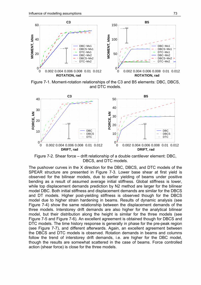
Influence of modelling assumptions 73
0 0.002 0.004 0.006 0.008 0.01 0.0120
20
40
60
ROTATION, rad
MO
ME
NT
, kN
m
C3
DBC−Mx1DBCS−Mx1DTC−Mx1DBC−Mx2DBCS−Mx2DTC−Mx2
0 0.002 0.004 0.006 0.008 0.01 0.012
0
50
100
150
ROTATION, rad
MO
ME
NT
, kN
m
B5
DBC−Mx1DBCS−Mx1DTC−Mx1DBC−Mx2DBCS−Mx2DTC−Mx2
Figure 7-1. Moment-rotation relationships of the C3 and B5 elements: DBC, DBCS,
and DTC models.
0 0.002 0.004 0.006 0.008 0.01 0.0120
10
20
30
40
DRIFT, rad
FO
RC
E, k
N
C3
DBCDBCSDTC
0 0.002 0.004 0.006 0.008 0.01 0.012
0
10
20
30
40
50
DRIFT, rad
FO
RC
E, k
N
B5
DBCDBCSDTC
Figure 7-2. Shear force – drift relationship of a double cantilever element: DBC,
DBCS, and DTC models. The pushover curves in the X direction for the DBC, DBCS, and DTC models of the SPEAR structure are presented in Figure 7-3. Lower base shear at first yield is observed for the bilinear models, due to earlier yielding of beams under positive bending as a result of assumed average initial stiffness. Global stiffness is lower, while top displacement demands prediction by N2 method are larger for the bilinear model DBC. Both initial stiffness and displacement demands are similar for the DBCS and DT models. Higher post-yielding stiffness is observed though for the DBCS model due to higher strain hardening in beams. Results of dynamic analysis (see Figure 7-4) show the same relationship between the displacement demands of the three models. Interstorey drift demands are also higher for the analytical bilinear model, but their distribution along the height is similar for the three models (see Figure 7-5 and Figure 7-6). An excellent agreement is obtained though for DBCS and DTC models. The time history response is generally in phase for the pre-peak region (see Figure 7-7), and different afterwards. Again, an excellent agreement between the DBCS and DTC models is observed. Rotation demands in beams and columns follow the trend of interstorey drift demands, i.e. are higher for the DBC model, though the results are somewhat scattered in the case of beams. Force controlled action (shear force) is close for the three models.

Influence of modelling assumptions 74
−200 −150 −100 −50 0 50 100 150 2000
50
100
150
200
250
300
350
TOP DISPLACEMENT, mm
BA
SE
SH
EA
R, k
NTRIANG
DBC−100XDBCS−100XDTC−100X1st yieldDCR=1N2 DEMAND
Figure 7-3. Pushover curves for the DBC, DBCS, and DTC models.
AL1 AL2 CA1 KA1 KA2 MO1 MO2 MEAN−150
−100
−50
0
50
100
150
EARTHQUAKE
TO
P D
ISP
LA
CE
ME
NT
D−T
X−R
3, m
m
DBCDBCSDTC
Figure 7-4. Top displacement demands in the X direction at the CM, dynamic
analysis, DBC, DBCS, and DTC models.

Influence of modelling assumptions 75
−0.02 −0.01 0 0.01 0.020
2
4
6
8
10
TX, rad
HE
IGH
T, m
MEAN DYNAMIC − 0.2g − CM
DBCDBCSDTC
−0.015−0.01−0.005 0 0.005 0.01 0.015
0
2
4
6
8
10
TY, rad
HE
IGH
T, m
MEAN DYNAMIC − 0.2g − CM
DBCDBCSDTC
Figure 7-5. Interstorey drift demands, dynamic analysis, DBC, DBCS, and DTC.
−0.02 −0.01 0 0.01 0.020
2
4
6
8
10
TX, rad
HE
IGH
T, m
N2 − SRSS − TRIANG − CM
DBCDBCSDTC
−0.015−0.01−0.005 0 0.005 0.01 0.015
0
2
4
6
8
10
TY, rad
HE
IGH
T, m
N2 − SRSS − TRIANG − CM
DBCDBCSDTC
Figure 7-6. Interstorey drift demands, pushover analysis, DBC, DBCS, and DTC.
0 2 4 6 8 10 12 14 16 18 20 22
−100
−50
0
50
100
TIME, s
D−T
X−R
3, m
m
TOP DISPLACEMENT TH, KA1−0
DBCDBCSDTC
Figure 7-7. Top displacement in the X direction time history: DBC, DBCS, and DTC.
It is known that the bilinear and trilinear idealisations of the member flexural response should provide similar results for high ductility demands when the yield rotation is the

Influence of modelling assumptions 76
same. However, substantial difference was observed for the SPEAR structure in the case of analytically derived bilinear and trilinear relationships. There are several factors responsible for the difference in the structural response. Due to different procedures used to derive the moment-rotation relationships for the two models, the yield rotation was slightly higher for the analytical bilinear case. Additionally, the bilinear model based on the assumption of average initial stiffness seriously alters the global element stiffness for unsymmetrical elements (beams), increasing the discrepancy between the DBC and DTC models. Conversely, an excellent agreement was observed between the DBCS and DTC models. This is attributed to the fact that the initial stiffness of the bilinear model represents an "effective" stiffness with respect to the trilinear model in the case of columns. Considering the very close initial global stiffness of the two models, and the importance of columns behaviour on the global structural response, the trilinear and bilinear models provided very close response.
7.2. Rigid offsets
For structural modelling of r.c. moment resisting frames it is usually required to account for the finite dimensions of beam-column joints, by considering rigid offsets for the interconnecting beam and column elements. Thus, FEMA356 requires beam-column joints to be represented as "stiff or rigid zone". On the other hand, joint deformations may be important, especially in the case of GLD frames, due to lack of joint transverse reinforcement and slippage of longitudinal reinforcement. Due to these reasons, Paulay and Priestley, 1992 "strongly recommend" that no allowance for rigid zones be made, though this is inferred with regard to lateral force analysis of ductile frames. However, centreline modelling of elements may be used as a simple way to account for both the reduction of stiffness and strength due to additional deformations in the joint regions for nonlinear structural assessment of GLD frames. The effect of rigid offsets on the force-deformation relationship of frame elements was studied on the examples of two elements: column C3, and beam B5 from the modelled structure. A double cantilever scheme was used to load the elements, so as to have double curvature bending. The centreline span of the double cantilever was the element span in the structure, i.e. 2.75m for the C3 column and 3m for the B5 beam. The moment-rotation relationships are those actually used for element in the structure model, and are presented in Figure 7-8 for the bilinear models DB (rigid offsets) and DBC (centreline model). A slight reduction of stiffness is noted for both elements. The effect of stiffness reduction for the centreline model is more pronounced for the shear force – drift relationship (see Figure 7-9), as its stiffness is proportional to the square of the span in this case. Additionally, a reduction of strength is present, proportional to the increase of distance between the plastic hinges. Beam force-displacement relationship is trilinear due to unsymmetrical bending resistance. Change of shear force - deflection stiffness for columns amount to 21 and 44% for first storey and second-third storey columns respectively, and from 9 to 19% for beams. Reduction of shear force capacity is of 10 and 20 % for the first and second-third storey columns, and from 4 to 9% for beams. It can be noticed that the differences between the centreline (DBC) and rigid offsets (DB) models will differ not only by the strength and stiffness of elements, but also by a different distribution of stiffness and strength.

Influence of modelling assumptions 77
0 0.002 0.004 0.006 0.008 0.01 0.0120
20
40
60
ROTATION, rad
MO
ME
NT
, kN
m
C3
DB−Mx1DBC−Mx1DB−Mx2DBC−Mx2
0 0.002 0.004 0.006 0.008 0.01 0.012
0
20
40
60
80
ROTATION, rad
MO
ME
NT
, kN
m
B5
DB−Mx1DBC−Mx1DB−Mx2DBC−Mx2
Figure 7-8. Moment-rotation relationships of the C3 and B5 elements: (DB vs. DBC).
0 0.002 0.004 0.006 0.008 0.01 0.0120
10
20
30
40
50
DRIFT, rad
FO
RC
E, k
N
C3
DBDBC
0 0.002 0.004 0.006 0.008 0.01 0.012
0
10
20
30
40
DRIFT, rad
FO
RC
E, k
N
B5
DBDBC
Figure 7-9. Influence of rigid offsets on the shear force – drift relationship of a double
cantilever element: DB vs. DBC models.
−200 −150 −100 −50 0 50 100 150 2000
50
100
150
200
250
300
350
TOP DISPLACEMENT, mm
BA
SE
SH
EA
R, k
N
TRIANG
DB−100XDBC−100X1st yieldDCR=1N2 DEMAND
Figure 7-10. Pushover curves for the DB and DBC models.

Influence of modelling assumptions 78
The pushover capacity curve of the SPEAR structure (see Figure 7-10) shows a significant reduction of strength and stiffness for the centreline model, as well as an increase of the top displacement demand by the N2 method. The same trend is observed from the dynamic analysis of the structures (see Figure 7-11).
AL1 AL2 CA1 KA1 KA2 MO1 MO2 MEAN−150
−100
−50
0
50
100
150
EARTHQUAKE
TO
P D
ISP
LA
CE
ME
NT
D−T
X−R
3, m
m
DBDBC
Figure 7-11. Influence of rigid offsets on top displacement demands in the X direction
at the CM, dynamic analysis.
−0.02 −0.01 0 0.01 0.020
2
4
6
8
10
TX, rad
HE
IGH
T, m
MEAN DYNAMIC − 0.2g − CM
DBDBC
−0.015−0.01−0.005 0 0.005 0.01 0.015
0
2
4
6
8
10
TY, rad
HE
IGH
T, m
MEAN DYNAMIC − 0.2g − CM
DBDBC
Figure 7-12. Influence of rigid offsets on interstorey drift demands, dynamic analysis.

Influence of modelling assumptions 79
−0.02 −0.01 0 0.01 0.020
2
4
6
8
10
TX, rad
HE
IGH
T, m
N2 − SRSS − TRIANG − CM
DBDBC
−0.015−0.01−0.005 0 0.005 0.01 0.015
0
2
4
6
8
10
TY, rad
HE
IGH
T, m
N2 − SRSS − TRIANG − CM
DBDBC
Figure 7-13. Influence of rigid offsets on interstorey drift demands, pushover analysis.
0 2 4 6 8 10 12 14 16 18 20 22
−100
−50
0
50
100
TIME, s
D−T
X−R
3, m
m
TOP DISPLACEMENT TH, KA1−0
DBDBC
Figure 7-14. Top displacement in the X direction time history: DB vs. DBC models.
The different distribution of stiffness and strength between the two models affects the distribution of inelastic drift demands, especially for the x direction (see Figure 7-12 and Figure 7-13). Higher displacement demands are imposed on the upper two storeys, as their stiffness and strength decrease more rapidly than that of the first storey columns (from geometry considerations). For the Y direction the effect of change in stiffness and strength distribution between the two models is not so pronounced, due to the strong column C6-15-24, which experiences significant plastic deformations at the base only, staying elastic at the upper floors. Thus, for the Y direction the effect of centreline dimensions of elements is to increase the drift demands, without affecting seriously their distribution along the height. The same trends for the drift demands in the X and Y directions are observed at the flexible and stiff edges of the structure, as well as for the distribution of plastic rotations in beams and columns along the building height. However, the shear force demand in beams and columns is less for the DBC model for all stories. Except for the increase of displacement demands for the DBC model, time history response is similar for the two models (see Figure 7-14). Correlation is best before the maximum deformations are reached (pre-peak region), and deteriorates after significant yielding of elements (post-peak time region).

Influence of modelling assumptions 80
The effect of rigid offsets showed the same trends for displacement, plastic rotation, and shear force demands in the case of the DT and DTC models (trilinear moment-rotation relationships for elements, with and without rigid offsets).
7.3. Post-yielding stiffness
The effect post-yielding stiffness of elements was studied on the base of the DT model (trilinear elements, rigid offsets, analytical post-yielding stiffness), by considering two additional models, DT1H and DT10H. Average values of analytical strain hardening of the DT model amounted to 0.56% and 0.86% for beams under positive and negative bending respectively, 1.8% for 250x250 columns, and 3.4% for 250x750 columns. The other two models used a fixed post-yielding stiffness of 1% (DT1H) and 10% (DT10H) for beams under positive bending and columns, and 3% (DT1H) and 20% (DT10H) for beams under negative bending. On the average, analytical predictions of post-yielding stiffness are between the two empirical models.
0 0.002 0.004 0.006 0.008 0.01 0.0120
20
40
60
ROTATION, rad
MO
ME
NT
, kN
m
C3
DT−Mx1DT1H−Mx1DT10H−Mx1DT−Mx2DT1H−Mx2DT10H−Mx2
0 0.002 0.004 0.006 0.008 0.01 0.012
0
50
100
150
ROTATION, rad
MO
ME
NT
, kN
mB5
DT−Mx1DT1H−Mx1DT10H−Mx1DT−Mx2DT1H−Mx2DT10H−Mx2
Figure 7-15. Moment-rotation relationships of the C3 and B5 elements: DT, DT1H,
and DT10H models. Moment-rotation relationships for the three models are presented in Figure 7-15 for the C3 and B5 elements. It may be noted that the absolute value of empirical post-yielding stiffness is sensitive to the secant stiffness to yield point. Thus, for slender elements (columns), the three models result in similar post-yielding stiffness. The difference is larger for beams under negative bending, due to both higher empirical post-yielding stiffness, and higher secant stiffness of T beams. A comparison of pushover curves for the three models is presented in Figure 7-16. Displacement demands by N2 method are seen to be insensitive to the amount of post-yielding stiffness, and so are the predictions of the dynamic analyses (see Figure 7-17). Distribution of interstorey drift demands along the height of the building is similar for the three models. In the case of the DT10H model, interstorey drift demands are slightly reduced for bottom two storeys and increased for the upper storey. The same trend along the height of the building is observed for plastic rotations in beams and columns. A very good agreement between the three models is observed also for the time history top displacement response, both for pre-peak and post-peak regions. The only important influence of the amount of post-yielding stiffness is the demand of elastic shear force in elements, these being higher for the DT10H model. Thus the increase of shear force in columns for the DT1H to the DT10H models ranges from 0 to 20%, with an average value of 10%.

Influence of modelling assumptions 81
−200 −150 −100 −50 0 50 100 150 2000
50
100
150
200
250
300
350
TOP DISPLACEMENT, mm
BA
SE
SH
EA
R, k
N
TRIANG
DT−100XDT1H−100XDT10H−100X1st yieldDCR=1N2 DEMAND
Figure 7-16. Pushover curves for the DT, DT1H, and DT10H models.
AL1 AL2 CA1 KA1 KA2 MO1 MO2 MEAN−80
−60
−40
−20
0
20
40
60
80
EARTHQUAKE
TO
P D
ISP
LA
CE
ME
NT
D−T
X−R
3, m
m
DTDT1HDT10H
Figure 7-17. Top displacement demands in the X direction at the CM, dynamic
analysis, DT, DT1H, and DT10H models.

Influence of modelling assumptions 82
−0.01 −0.005 0 0.005 0.010
2
4
6
8
10
TX, rad
HE
IGH
T, m
MEAN DYNAMIC − 0.2g − CM
DTDT1HDT10H
−0.01 −0.005 0 0.005 0.01
0
2
4
6
8
10
TY, rad
HE
IGH
T, m
MEAN DYNAMIC − 0.2g − CM
DTDT1HDT10H
Figure 7-18. Interstorey drift demands, dynamic analysis, DT, DT1H, and DT10H
models.
−0.015−0.01−0.005 0 0.005 0.01 0.0150
2
4
6
8
10
TX, rad
HE
IGH
T, m
N2 − SRSS − TRIANG − CM
DTDT1HDT10H
−0.01 −0.005 0 0.005 0.01
0
2
4
6
8
10
TY, rad
HE
IGH
T, m
N2 − SRSS − TRIANG − CM
DTDT1HDT10H
Figure 7-19. Interstorey drift demands, pushover analysis, DT, DT1H, and DT10H
models. The amount of post-yielding stiffness showed to have little influence on the displacement demands of the SPEAR structure. As the first two vibration periods of the structure are higher than the characteristic period of the ground motions, the equal displacement rule applies in the N2 method. Therefore, the displacement demands are insensitive to the amount of post-yielding stiffness. However, different values of strain hardening for particular actions (positive and negative beam bending moments) may influence the distribution of interstorey drift demands by altering the ratio of post-yielding moment demands among the elements. This effect was small for this particular case, as the strength hierarchy was the same for the three models (weak columns and beams under positive bending). The only significant effect of higher post-yielding stiffness for the SPEAR building is the increase of elastic shear demands.

Influence of modelling assumptions 83
0 2 4 6 8 10 12 14 16 18 20 22
−50
0
50
TIME, s
D−T
X−R
3, m
m
TOP DISPLACEMENT TH, KA1−0
DTDT1HDT10H
Figure 7-20. Top displacement in the X direction time history: DT, DT1H, and DT10H
models.
7.4. Pinching
Significant pinching effect may be experienced by both beams and columns in GLD frames due to slippage of longitudinal reinforcement in the beam-column joint region. Modelling of pinching in the CANNY program is based on a reduction of reloading stiffness after yielding occurred in the opposite direction. Reloading stiffness is proportional to ( )/y m
λθ θ , where θy is the yield rotation, θm is the maximum rotation
attained previously, and λ is a pinching factor. Thus, according to this model, no pinching effect is introduced before yielding of the element. The effect of pinching was studied on the DT model (no pinching), by considering two new models, DTP (moderate pinching) and DTP1 (strong pinching), with 0.5 and 1.0 pinching factors, respectively, applied to both beams and columns. A comparison of the cyclic behaviour of the C3 and B5 double cantilever elements for the DT and DTP models is presented in Figure 7-21.
−0.01 −0.005 0 0.005 0.01−50
0
50
DRIFT, rad
FO
RC
E, k
N
C3
DTDTP
−0.04 −0.02 0 0.02 0.04
−40
−20
0
20
40
DRIFT, rad
FO
RC
E, k
N
B5
DTDTP
Figure 7-21. Force-displacement relationships for the C3 and B5 elements: DT and
DTP models. As the same moment-rotation envelopes are used for models with and without pinching, the pushover analysis will yield identical results for the three models, and are not presented here. Maximum top displacement demands of dynamic analysis for the DT and DTP models are shown in Figure 7-22. Very limited effect of pinching

Influence of modelling assumptions 84
behaviour is noted. The same conclusion is inferred from the interstorey drift demands (Figure 7-23), and the top displacement time histories (Figure 7-24). As most of the beams are yielding only in positive bending, the pinching behaviour is not triggered on for these elements. Inelastic structural response is dictated by the behaviour of columns. With the exception of the CA1 earthquake record, column response is characterised by few (one-two) full inelastic excursions, followed by a number of cycles of smaller amplitude. Pinching behaviour is triggered after the first yielding, and affects generally only the smaller inner loops (see Figure 7-25). However, the CA1 record (see Annex II) is characterised by long duration and two distinct regions of maximum response. For this record, the pinching model results in slightly higher rotation and displacement demands, as the pinching behaviour affects the full cycles under the second group of strong motion.
AL1 AL2 CA1 KA1 KA2 MO1 MO2 MEAN−80
−60
−40
−20
0
20
40
60
80
EARTHQUAKE
TO
P D
ISP
LA
CE
ME
NT
D−T
X−R
3, m
m
DTDTP
Figure 7-22. Top displacement demands in the X direction at the CM, dynamic
analysis, DT and DTP models.
−0.01 −0.005 0 0.005 0.010
2
4
6
8
10
TX, rad
HE
IGH
T, m
MEAN DYNAMIC − 0.2g − CM
DTDTP
−0.01 −0.005 0 0.005 0.01
0
2
4
6
8
10
TY, rad
HE
IGH
T, m
MEAN DYNAMIC − 0.2g − CM
DTDTP
Figure 7-23. Interstorey drift demands, dynamic analysis, DT and DTP models.

Influence of modelling assumptions 85
0 2 4 6 8 10 12 14 16 18 20 22
−50
0
50
TIME, s
D−T
X−R
3, m
m
TOP DISPLACEMENT TH, KA1−0
DTDTP
Figure 7-24. Top displacement in the X direction time history: DT and DTP models.
−0.01 −0.005 0 0.005 0.01−60
−40
−20
0
20
40
60
My1 − ROTATION, rad
MO
ME
NT
, kN
m
C3 − 0.2g − KA1−0
DTDTP
−0.015−0.01−0.005 0 0.005 0.01−60
−40
−20
0
20
40
60
My1 − ROTATION, rad
MO
ME
NT
, kN
m
C3 − 0.2g − CA1−0
DTDTP
Figure 7-25. Moment-rotation behaviour of the C3 column for the KA1 and CA1
ground motions. The effect of stronger pinching was considered for the DTP1 model, but insignificant differences were observed in comparison with the "moderate" pinching model DTP. Higher intensity of earthquake input (0.3g) was considered additionally for the DT and DTP models, but the structural response followed the trend of the lower intensity analyses.
7.5. Beam effective width
It was shown in chapter 4.3 that important variations of the beam effective widths may be predicted according to different sources. The effect of beam effective widths on the global response of the SPEAR structure was studied on the base of the DT model (EC8 effective width). The DTF model was obtained by considering FEMA356 effective widths. As it was discussed previously the effect of higher beam effective width is the increase of initial stiffness and of flexural capacity under negative bending moments. Yielding curvature and positive moment capacity show little variation with beam effective width (see Figure 7-26).
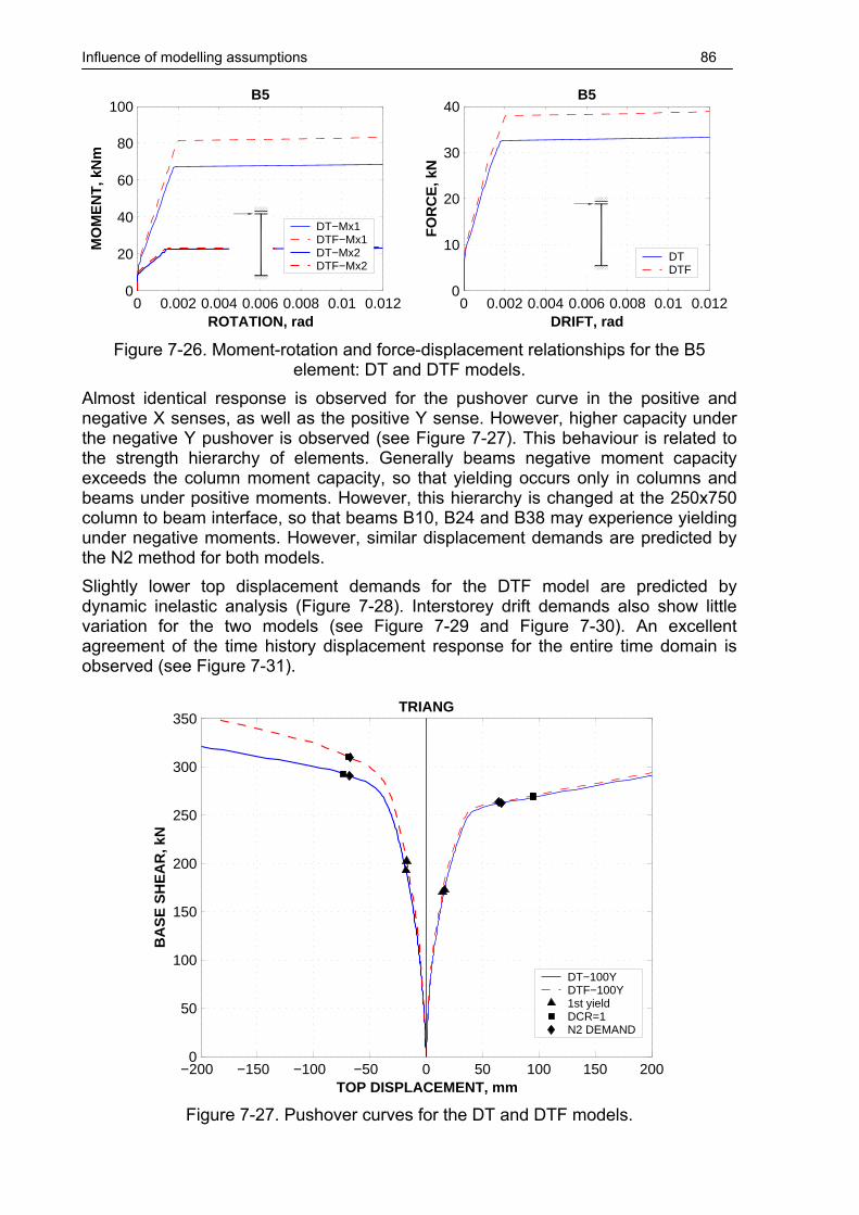
Influence of modelling assumptions 86
0 0.002 0.004 0.006 0.008 0.01 0.0120
20
40
60
80
100
ROTATION, rad
MO
ME
NT
, kN
mB5
DT−Mx1DTF−Mx1DT−Mx2DTF−Mx2
0 0.002 0.004 0.006 0.008 0.01 0.012
0
10
20
30
40
DRIFT, rad
FO
RC
E, k
N
B5
DTDTF
Figure 7-26. Moment-rotation and force-displacement relationships for the B5
element: DT and DTF models. Almost identical response is observed for the pushover curve in the positive and negative X senses, as well as the positive Y sense. However, higher capacity under the negative Y pushover is observed (see Figure 7-27). This behaviour is related to the strength hierarchy of elements. Generally beams negative moment capacity exceeds the column moment capacity, so that yielding occurs only in columns and beams under positive moments. However, this hierarchy is changed at the 250x750 column to beam interface, so that beams B10, B24 and B38 may experience yielding under negative moments. However, similar displacement demands are predicted by the N2 method for both models. Slightly lower top displacement demands for the DTF model are predicted by dynamic inelastic analysis (Figure 7-28). Interstorey drift demands also show little variation for the two models (see Figure 7-29 and Figure 7-30). An excellent agreement of the time history displacement response for the entire time domain is observed (see Figure 7-31).
−200 −150 −100 −50 0 50 100 150 2000
50
100
150
200
250
300
350
TOP DISPLACEMENT, mm
BA
SE
SH
EA
R, k
N
TRIANG
DT−100YDTF−100Y1st yieldDCR=1N2 DEMAND
Figure 7-27. Pushover curves for the DT and DTF models.

Influence of modelling assumptions 87
AL1 AL2 CA1 KA1 KA2 MO1 MO2 MEAN−80
−60
−40
−20
0
20
40
60
80
EARTHQUAKE
TO
P D
ISP
LA
CE
ME
NT
D−T
X−R
3, m
m
DTDTF
Figure 7-28. Top displacement demands in the X direction at the CM, dynamic
analysis, DT and DTF models.
−0.01 −0.005 0 0.005 0.010
2
4
6
8
10
TX, rad
HE
IGH
T, m
MEAN DYNAMIC − 0.2g − CM
DTDTF
−0.01 −0.005 0 0.005 0.01
0
2
4
6
8
10
TY, rad
HE
IGH
T, m
MEAN DYNAMIC − 0.2g − CM
DTDTF
Figure 7-29. Interstorey drift demands, dynamic analysis, DT and DTF models.
Seismic response of the SPEAR building showed to be insensitive to comparatively large variations in beam effective widths, as it did not alter the strength hierarchy of elements. However, the different assumptions of effective widths may be important for other structures, as higher beam capacities promote a soft-storey effect. It may also be important in the case of column strengthening as a rehabilitation measure.

Influence of modelling assumptions 88
−0.015−0.01−0.005 0 0.005 0.01 0.0150
2
4
6
8
10
TX, rad
HE
IGH
T, m
N2 − SRSS − TRIANG − CM
DTDTF
−0.01 −0.005 0 0.005 0.01
0
2
4
6
8
10
TY, rad
HE
IGH
T, m
N2 − SRSS − TRIANG − CM
DTDTF
Figure 7-30. Interstorey drift demands, pushover analysis, DT and DTF models.
0 2 4 6 8 10 12 14 16 18 20 22
−50
0
50
TIME, s
D−T
X−R
3, m
m
TOP DISPLACEMENT TH, KA1−0
DTDTF
Figure 7-31. Top displacement in the X direction time history: DT and DTF models.
7.6. M-M-N interaction
The influence of biaxial moment demand and axial force variation in columns was studied by considering multispring elements for columns. One-component trilinear modelling of columns (DT) overestimates their biaxial strength. It also fails to account for the variation of axial force due to earthquake loading, accounting for the gravitational axial effect only. Two models accounting for these effects were considered: DMS and DMSa, based on a multispring (fibre) modelling of columns (see chapter 4.2). The same one-component modelling of beams was used in all three cases. Material stress-strain relationships based on design specifications (material model D) was applied. Plastic deformations are concentrated at the element ends for the multispring modelling, elastic behaviour being assumed for line element. A slight modification of the steel stress-strain relationship was used for the DMSa model, as suggested in the CANNY user manual, to counterbalance the lower displacements at yield predicted by the multispring element.

Influence of modelling assumptions 89
050
100150200250300350400
0 0.0025 0.005 0.0075 0.01STRAIN
STR
ESS
N/m
m2
DMSDMSa
Figure 7-32. "Adjusted" stress-strain relationship for steel springs in the DMSa model. Figure 7-33 presents the monotonic and cyclic force-displacement relationships for the C3 double cantilever column. The trilinear and multi-spring column models are in close agreement, the DMSa model showing better correlation of the yield displacement with the trilinear idealisation. Under cyclic loading there is less difference between the DMS and DMSa models. Multispring models present a pinching behaviour. This is caused by cracks in the tension zone staying open during moment reversals due to large plastic strain of longitudinal reinforcement, so that bending moment is resisted by a steel couple alone over a portion of the loading history (Filippou et al, 1992). Less post-yielding stiffness is present in the multispring models.
0 0.002 0.004 0.006 0.008 0.01 0.0120
10
20
30
40
50
DRIFT, rad
FO
RC
E, k
N
C3
DTDMSDMSa
−0.01 −0.005 0 0.005 0.01
−50
0
50
DRIFT, rad
FO
RC
E, k
N
C3
DTDMSDMSa
Figure 7-33. Monotonic and cyclic shear force - drift relationships of the C3 element:
DT, DMS, and DMSa models. Static inelastic response of the DT, DMS, and DMSa models is shown in Figure 7-34. Initial stiffness is in close agreement between the models, so are the displacement demands predicted by the N2 method. the post yielding stiffness is somewhat different, but the base shear at the attainment of the ultimate rotation capacity in critical elements (DCR=1) is very similar among the three models. Higher top displacement demands in the X direction (Figure 7-35), but slightly smaller in the Y direction are predicted by the dynamic analyses for the multispring models. Interstorey drift demands present the same directional trend, higher drift demands being observed for the first storey in X direction (see Figure 7-36). Pushover predictions of interstorey drift demands do not reflect exactly these small differences though (Figure 7-37). Top displacement time history was generally in phase for the pre-peak range, but different for post-peak range. Column rotations demands

Influence of modelling assumptions 90
followed the trends of interstorey drifts, while the elastic shear force demand was close fro the three models.
−200 −150 −100 −50 0 50 100 150 2000
50
100
150
200
250
300
350
TOP DISPLACEMENT, mm
BA
SE
SH
EA
R, k
N
TRIANG
DT−100XDMS−100XDMSa−100X1st yieldDCR=1N2 DEMAND
Figure 7-34. Pushover curves for the DT, DMS, and DMSa models.
AL1 AL2 CA1 KA1 KA2 MO1 MO2 MEAN−100
−50
0
50
100
EARTHQUAKE
TO
P D
ISP
LA
CE
ME
NT
D−T
X−R
3, m
m
DTDMSDMSa
Figure 7-35. Top displacement demands in the X direction at the CM, dynamic
analysis, DT, DMS, and DMSa models.

Influence of modelling assumptions 91
−0.01 −0.005 0 0.005 0.010
2
4
6
8
10
TX, rad
HE
IGH
T, m
MEAN DYNAMIC − 0.2g − CM
DTDMSDMSa
−0.01 −0.005 0 0.005 0.01
0
2
4
6
8
10
TY, rad
HE
IGH
T, m
MEAN DYNAMIC − 0.2g − CM
DTDMSDMSa
Figure 7-36. Interstorey drift demands, dynamic analysis, DT, DMS, and DMSa
models.
−0.015−0.01−0.005 0 0.005 0.01 0.0150
2
4
6
8
10
TX, rad
HE
IGH
T, m
N2 − SRSS − TRIANG − CM
DTDMSDMSa
−0.01 −0.005 0 0.005 0.01
0
2
4
6
8
10
TY, rad
HE
IGH
T, m
N2 − SRSS − TRIANG − CM
DTDMSDMSa
Figure 7-37. Interstorey drift demands, pushover analysis (DT, DMS, and DMSa).
0 2 4 6 8 10 12 14 16 18 20 22
−50
0
50
TIME, s
D−T
X−R
3, m
m
TOP DISPLACEMENT TH, KA1−0
DTDMSDMSa
Figure 7-38. Top displacement in the X direction time history: DT, DMS, and DMSa
models.

Influence of modelling assumptions 92
Following the biaxial response of the columns of the SPEAR structure under bidirectional seismic input, it may be noticed that it is not uncommon that the maximum or close to maximum response is obtained for the same time instant (see Figure 7-39). Biaxial moment capacity is thus overpredicted by the DT model. DMS and DMSa models, show a reduction of moment capacity under biaxial demand, and an increase of the deformations (see Figure 7-40). The effect of varying axial force at the exterior columns will add to the effects of biaxial moment demand.
−0.01 −0.005 0 0.005 0.01
−0.01
−0.005
0
0.005
0.01
My1 − ROTATION, rad
Mx1
− R
OT
AT
ION
, rad
C3 − 0.2g − AL1−0
DTDMSDMSa
−60 −40 −20 0 20 40 60
−60
−40
−20
0
20
40
60
My1 − Moment, kNm
Mx1
− M
om
ent,
kN
m
C3 − 0.2g − AL1−0
DTDMSDMSa
Figure 7-39. Biaxial rotation and moment demands at the C3 column bottom end: DT,
DMS, and DMSa models.
−0.01 −0.005 0 0.005 0.01−60
−40
−20
0
20
40
60
Mx1 − ROTATION, rad
MO
ME
NT
, kN
m
C3 − 0.2g − AL1−0
DTDMSDMSa
−0.01 −0.005 0 0.005 0.01
−60
−40
−20
0
20
40
60
My1 − ROTATION, rad
MO
ME
NT
, kN
m
C3 − 0.2g − AL1−0
DTDMSDMSa
Figure 7-40. Moment-rotation response at the C3 column bottom end: DT, DMS, and
DMSa models. M-M-N interaction is shown to affect the response of columns when they represent the weak links in the structure. Strength and stiffness degradation is to be expected for the models accounting for M-M-N interaction, leading to higher displacement demands. Though global structural response is not seriously affected by consideration of biaxial moment and axial force interaction, higher interstorey drifts are expected in lower stories due to higher axial forces in columns.

Influence of modelling assumptions 93
7.7. Strength degradation
Element models considered so far did not include any strength degradation. Attainment of the ultimate deformations in elements is then compared to the demands obtained from analysis. Modelling of strength degradation provide a direct way to check for the attainment of structural collapse. However, negative stiffness is prone to numerical problems, which makes it less attractive. Influence of strength degradation modelling on the structural response was studied on two models: DMS and DDMS. The same characteristic strength of materials was used in both cases, but concrete softening after maximum stress was considered for the DDMS model (see Figure 4-1, material model DD). As little if no strength degradation is expected for beams, it was explicitly modelled for columns only (multispring elements). Influence of concrete softening on the force-deflection relationship for the double cantilever C3 column is presented in Figure 7-41. The multispring element modelling is able to reflect strength degradation under both monotonic and cyclic loading.
0 0.002 0.004 0.006 0.008 0.01 0.0120
10
20
30
40
50
DRIFT, rad
FO
RC
E, k
N
C3
DMSDDMS
−0.01 −0.005 0 0.005 0.01
−50
0
50
DRIFT, rad
FO
RC
E, k
NC3
DMSDDMS
Figure 7-41. Monotonic and cyclic shear force - drift relationships of the C3 element:
DMS and DDMS models. The pushover curves for the X direction of the SPEAR building are presented in Figure 7-42. A similar behaviour is observed up to the attainment of ultimate rotations in columns (not shown here, but close to the N2 demand, see also Figure 7-34), followed by a rapid strength degradation in the case of the DDMS model. Close predictions of the displacements demands by N2 method are also noticed. Less global strength degradation is present for the Y direction. Average dynamic displacements demands are also close for the two models, a slight increase is though present for the "most degrading" +X direction. Distribution of interstorey drift demands in the X direction are much changed between the two models (see Figure 7-44). As strength and stiffness degradation under cyclic loading are bigger for the first storey columns due to higher axial load, a considerable increase of first storey drifts and decrease of the two upper stories drifts in the X direction occurred for the DDMS model. The redistribution of the interstorey drift demands from the upper two stories to the first one is present also in the Y direction, but at a much smaller scale, due to the strong 250x750 column, which inhibits a first storey plastic mechanism. Prediction of interstorey drift distribution by pushover analysis for the DDMS model (see Figure 7-45) is in worse agreement than for other cases, as the effect of cyclic degradation of strength and stiffness is not included in the pushover analysis.

Influence of modelling assumptions 94
Rotation demands in beams are similar for the two models, while those in columns follow the trend of interstorey drift demands (higher in the first and lower in the upper stories for the DDMS model). Shear force demands show close values between the two models.
−200 −150 −100 −50 0 50 100 150 2000
50
100
150
200
250
300
350
TOP DISPLACEMENT, mm
BA
SE
SH
EA
R, k
N
TRIANG
DMS−100XDDMS−100X1st yieldN2 DEMAND
Figure 7-42. Pushover curves for the DMS and DDMS models.
AL1 AL2 CA1 KA1 KA2 MO1 MO2 MEAN−100
−50
0
50
100
EARTHQUAKE
TO
P D
ISP
LA
CE
ME
NT
D−T
X−R
3, m
m
DMSDDMS
Figure 7-43. Top displacement demands in the X direction at the CM, dynamic
analysis, DMS and DDMS models. Top displacement time-history was in good agreement between the two models for the pre-peak range. Though being generally in-phase for the post-peak range of response, higher permanent deformations were sometimes observed for the degrading model (see Figure 7-46). Even when higher seismic intensity was considered (0.3g) top displacement demands did not increased much for the degrading model. However, the distribution of interstorey drifts (and damage thereof) followed the same trends of concentrating

Influence of modelling assumptions 95
in damage-prone first storey (due to higher axial load on columns) for both X and Y directions.
−0.015−0.01−0.005 0 0.005 0.01 0.0150
2
4
6
8
10
TX, rad
HE
IGH
T, m
MEAN DYNAMIC − 0.2g − CM
DMSDDMS
−0.01 −0.005 0 0.005 0.01
0
2
4
6
8
10
TY, rad
HE
IGH
T, m
MEAN DYNAMIC − 0.2g − CM
DMSDDMS
Figure 7-44. Interstorey drift demands, dynamic analysis, DMS and DDMS models.
−0.015−0.01−0.005 0 0.005 0.01 0.0150
2
4
6
8
10
TX, rad
HE
IGH
T, m
N2 − SRSS − TRIANG − CM
DMSDDMS
−0.01 −0.005 0 0.005 0.01
0
2
4
6
8
10
TY, rad
HE
IGH
T, m
N2 − SRSS − TRIANG − CM
DMSDDMS
Figure 7-45. Interstorey drift demands, pushover analysis, DMS and DDMS models.
0 2 4 6 8 10 12 14 16 18 20 22−100
−50
0
50
100
TIME, s
D−T
X−R
3, m
m
TOP DISPLACEMENT TH, KA1−0
DMSDDMS
Figure 7-46. Top displacement in the X direction time history: DMS and DDMS.
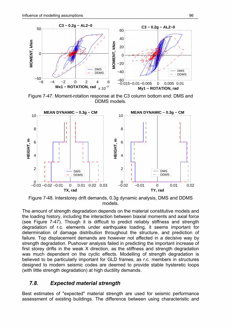
Influence of modelling assumptions 96
−6 −4 −2 0 2 4 6
x 10−3
−50
0
50
Mx1 − ROTATION, rad
MO
ME
NT
, kN
mC3 − 0.2g − AL2−0
DMSDDMS
−0.015−0.01−0.005 0 0.005 0.01−60
−40
−20
0
20
40
60
My1 − ROTATION, rad
MO
ME
NT
, kN
m
C3 − 0.2g − AL2−0
DMSDDMS
Figure 7-47. Moment-rotation response at the C3 column bottom end: DMS and
DDMS models.
−0.03 −0.02 −0.01 0 0.01 0.02 0.030
2
4
6
8
10
TX, rad
HE
IGH
T, m
MEAN DYNAMIC − 0.3g − CM
DMSDDMS
−0.02 −0.01 0 0.01 0.02
0
2
4
6
8
10
TY, rad
HE
IGH
T, m
MEAN DYNAMIC − 0.3g − CM
DMSDDMS
Figure 7-48. Interstorey drift demands, 0.3g dynamic analysis, DMS and DDMS
models. The amount of strength degradation depends on the material constitutive models and the loading history, including the interaction between biaxial moments and axial force (see Figure 7-47). Though it is difficult to predict reliably stiffness and strength degradation of r.c. elements under earthquake loading, it seems important for determination of damage distribution throughout the structure, and prediction of failure. Top displacement demands are however not affected in a decisive way by strength degradation. Pushover analysis failed in predicting the important increase of first storey drifts in the weak X direction, as the stiffness and strength degradation was much dependent on the cyclic effects. Modelling of strength degradation is believed to be particularly important for GLD frames, as r.c. members in structures designed to modern seismic codes are deemed to provide stable hysteretic loops (with little strength degradation) at high ductility demands.
7.8. Expected material strength
Best estimates of "expected" material strength are used for seismic performance assessment of existing buildings. The difference between using characteristic and

Influence of modelling assumptions 97
expected material strength was studied on the DDMS and EMS models (material models DD and E respectively, see Figure 4-1). The increase in flexural capacity of elements due to higher material strength is dictated by the increase of steel yield strength, and is approximately 10% for both beams and columns. Monotonic and cyclic shear force – deflection relationships for the C3 double cantilever column are shown in Figure 7-49.
0 0.002 0.004 0.006 0.008 0.01 0.0120
10
20
30
40
50
DRIFT, rad
FO
RC
E, k
N
C3
DDMSEMS
−0.01 −0.005 0 0.005 0.01
−50
0
50
DRIFT, radF
OR
CE
, kN
C3
DDMSEMS
Figure 7-49. Monotonic and cyclic shear force - drift relationships of the C3 element:
DDMS and EMS models. Beside the increase of flexural capacity, higher concrete strength is seen to improve element rotation capacity and diminish strength degradation under cyclic loading for columns, whose failure was controlled by concrete crushing. However, the pinching effect due to axial force is increased for EMS columns. Pushover curves of the SPEAR building for the X direction of loading are presented in Figure 7-50. Initial global stiffness is close for the DDMS and EMS models. An increase of the base shear at first yield and maximum base shear for the EMS models is noted, of the order of 10%. Additionally, an increase of deformations at the beginning of significant strength degradation is noticed for the EMS model. Close top displacement demands are predicted by the N2 method for the DDMS and EMS models. Mean of dynamic top displacement demands are however lower in the case of EMS model (see Figure 7-51), for both X and Y directions. Increase of concrete strength (EMS) provides more uniform interstorey drift demands in comparison with the DDMS model for the weak (X) direction (see Figure 7-52), reducing the potential for a storey plastic mechanism. This trend is observed also for the pushover predictions of interstorey drift demands (see Figure 7-53). However, static inelastic drift distributions along the height of the structure are in poor agreement with dynamic results, due to the important effect of cyclic stiffness and strength degradation for both models. A good agreement between the top displacement time-history is noticed for the two models, for both pre- and post-peak ranges (Figure 7-54). Lower permanent displacements are generally noted for the EMS model, due to more stable hysteresis loops.

Influence of modelling assumptions 98
−200 −150 −100 −50 0 50 100 150 2000
50
100
150
200
250
300
350
TOP DISPLACEMENT, mm
BA
SE
SH
EA
R, k
N
TRIANG
DDMS−100XEMS−100X1st yieldN2 DEMAND
Figure 7-50. Pushover curves for the DDMS and EMS models.
Close estimates for beam rotation demands are noted for both models. Column rotation demands follow the trends of interstorey drift distributions along the height of the building. The increase of elastic shear force demands in elements following the approximately 10% increase of flexural capacities for beams and columns is observed.
AL1 AL2 CA1 KA1 KA2 MO1 MO2 MEAN−100
−50
0
50
100
EARTHQUAKE
TO
P D
ISP
LA
CE
ME
NT
D−T
X−R
3, m
m
DDMSEMS
Figure 7-51. Top displacement demands in the X direction at the CM, dynamic
analysis, DDMS and EMS models.

Influence of modelling assumptions 99
−0.015−0.01−0.005 0 0.005 0.01 0.0150
2
4
6
8
10
TX, rad
HE
IGH
T, m
MEAN DYNAMIC − 0.2g − CM
DDMSEMS
−0.01 −0.005 0 0.005 0.01
0
2
4
6
8
10
TY, rad
HE
IGH
T, m
MEAN DYNAMIC − 0.2g − CM
DDMSEMS
Figure 7-52. Interstorey drift demands, dynamic analysis, DDMS and EMS models.
−0.015−0.01−0.005 0 0.005 0.01 0.0150
2
4
6
8
10
TX, rad
HE
IGH
T, m
N2 − SRSS − TRIANG − CM
DDMSEMS
−0.01 −0.005 0 0.005 0.01
0
2
4
6
8
10
TY, rad
HE
IGH
T, m
N2 − SRSS − TRIANG − CM
DDMSEMS
Figure 7-53. Interstorey drift demands, pushover analysis, DDMS and EMS models.
0 2 4 6 8 10 12 14 16 18 20 22−100
−50
0
50
100
TIME, s
D−T
X−R
3, m
m
TOP DISPLACEMENT TH, KA1−0
DDMSEMS
Figure 7-54. Top displacement in the X direction time history: DDMS and EMS.

Influence of modelling assumptions 100
−6 −4 −2 0 2 4 6
x 10−3
−60
−40
−20
0
20
40
60
Mx1 − ROTATION, rad
MO
ME
NT
, kN
mC3 − 0.2g − AL2−0
DDMSEMS
−0.015−0.01−0.005 0 0.005 0.01−60
−40
−20
0
20
40
60
My1 − ROTATION, rad
MO
ME
NT
, kN
m
C3 − 0.2g − AL2−0
DDMSEMS
Figure 7-55. Moment-rotation response at the C3 column bottom end: DDMS and
EMS models. Though lower ultimate concrete strains are predicted for the higher strength concrete (E material model, see Figure 4-1), increase of concrete strength leads to more stable hysteresis loops (see Figure 7-55) under earthquake loading for columns. Less stiffness and strength degradation was thus observed for the first storey column in the EMS model in comparison with the DDMS one. This had an effect of more favourable plastic mechanism for the weaker X direction, and lower displacement demands for the EMS model. The increase of flexural capacities and elastic shear demands in elements approximately followed the increase of steel yield strength.
7.9. Modelling uncertainties
Structural models considered in this study were based on assumptions commonly adopted by engineering profession for evaluation of seismic performance of r.c. structures. Adoption of one modelling parameter or another is often based on personal experience, engineering judgement, and available computer codes, and is consequently largely subjective. Some of the modelling assumptions were shown not to influence significantly the results of analyses. However, the importance of each modelling parameters are expected to change for different structural designs. The ensemble of dynamic interstorey drift demands for different models of the SPEAR building is presented in Figure 7-56, and that for pushover curves in the X direction is shown in Figure 7-57. Large scatter is observed both in estimates of global structural properties (stiffness and strength), and in demands (top displacements and interstorey drifts). Large uncertainties were observed as well for estimation of joint shear resistance and element shear strength. When these components represent the weak link, evaluation of seismic response will impose additional scatter in results. Experimental validation of the different approaches is expected to have an important contribution to the development of analytical procedures for seismic assessment of engineering structures. Much work is still needed, however.

Influence of modelling assumptions 101
−60 −40 −20 0 20 40 60
1
2
3
TX, mm
ST
OR
EY
MEAN DYNAMIC − 0.2g − CMDBDBCDTDTCDBCSDT1HDT10HDTPBDTPDTP1DTFDMSDMSaDDMSEMSETCPEFCP
Figure 7-56. Scatter of interstorey drift demands for the set of models considered.
−200 −150 −100 −50 0 50 100 150 2000
50
100
150
200
250
300
350
TOP DISPLACEMENT, mm
BA
SE
SH
EA
R, k
N
TRIANG
DB−100XDBC−100XDT−100XDTC−100XDBCS−100XDT1H−100XDT10H−100XDTPB−100XDTP−100XDTP1−100XDTF−100XDMS−100XDMSa−100XDDMS−100XEMS−100XETCP−100XEFCP−100X1st yieldN2 DEMAND
Figure 7-57. Pushover curves in the X direction for the set of models considered.
"Best estimate" models 102
8. "BEST ESTIMATE" MODELS
8.1. Comparison to experimental tests
Seismic performance of the SPEAR building is strongly dependent on the behaviour of columns, which represent the weakest link in the structure. To verify the analytical models used in this study, and possibly choose the best one, a comparison to experimental behaviour of two columns similar to the ones of the SPEAR building was performed. Experimental data was extracted from the column database at the University of Washington ("Database", n.d.). Test results are presented in the form of load-displacement values of an equivalent cantilever column. The first column was the No.1 specimen tested by Nosho, Stanton and MacRae in 1996. The column had a 279x279 mm square cross-section, four 16 mm longitudinal bars, and 6.35 mm stirrups spaced at 228.6 mm. Element was tested cyclically as a cantilever of 2134 mm length, with an applied axial compressive load of 1076 kN (ν=0.34). Measured concrete strength amounted to 40.6 N/mm2, while the longitudinal steel yield strength of 407 N/mm2. The second column was the No. 12 specimen tested by Atalay and Penzien in 1975. It had a 305x305 mm square cross-section, four 22 mm diameter longitudinal bars, and 9.5 mm diameter stirrups spaced at 127 mm. Cyclic loading history was applied as well. Testing configuration was of a double ended element, with an applied axial compressive load of 801 kN (ν=0.27). Material properties were: 31.8 N/mm2 concrete compressive strength and 363 N/mm2 longitudinal steel yield strength. The clear span of the equivalent cantilever was of 1676 mm. The column of Nosho et al. is the closest to the SPEAR building 250x250 columns, including the widely spaced stirrups. As there was only one test reported, it was decided to include one more column (the one of Atalay and Penzien) in the comparison. Four analytical models were considered for each column: bilinear (BIL), trilinear (TRI), multispring (MS), and fibre (FIB), as described in chapter 4.2. Takeda hysteretic rules were used for the bilinear and trilinear one-component models. Reported material strength was used, supplemented by derived stress-strain relationships corresponding to degrading concrete and strain-hardening steel (material model E). Due to large spacing of stirrups, concrete core was considered unconfined for the Nosho column. In the case of Atalay specimen, core concrete stress-strain relationship was obtained considering confined conditions (Mander et al., 1988). Cover was modelled as unconfined spalling concrete in both cases. Both monotonic and cyclic loading was applied to each of the analytical CANNY models, for an equivalent double cantilever element. The comparison of analytical monotonic results to envelope of experimental test for the Nosho et al. specimen is presented in Figure 8-1. A generally good agreement is observed for all the models up to the maximum force, the MS element presenting though lower deformation at yield. There are important differences between the analytical predictions of ultimate displacement capacity and the experimental observations for the BI, TRI, and MS models. This is attributed to the assumed value of the plastic hinge length. Cyclic analytical vs. experimental response is presented in Figure 8-2 for the entire loading history and in Figure 8-3 for a single cycle (for clarity).

"Best estimate" models 103
0 0.005 0.01 0.015 0.020
20
40
60
DRIFT, rad
FO
RC
E, k
N
Nosho
EXPBILTRI
0 0.005 0.01 0.015 0.02
0
20
40
60
DRIFT, rad
FO
RC
E, k
N
Nosho
EXPMSFIB
Figure 8-1. Analytical monotonic base shear – drift relationships vs. experimental
envelope for the Nosho et al. specimen.
−0.02 −0.01 0 0.01 0.02−100
−50
0
50
100
DRIFT, rad
FO
RC
E, k
N
Nosho
EXPBILTRI
−0.02 −0.01 0 0.01 0.02
−100
−50
0
50
100
DRIFT, rad
FO
RC
E, k
N
Nosho
EXPMSFIB
Figure 8-2. Analytical vs. experimental cyclic base shear – drift relationships for the
Nosho et al. specimen.
−0.02 −0.01 0 0.01 0.02−100
−50
0
50
100
DRIFT, rad
FO
RC
E, k
N
Nosho
EXPBILTRI
−0.02 −0.01 0 0.01 0.02
−100
−50
0
50
100
DRIFT, rad
FO
RC
E, k
N
Nosho
EXPMSFIB
Figure 8-3. Analytical vs. experimental cyclic base shear – drift relationships for the
Nosho et al. specimen for a single loading cycle.

"Best estimate" models 104
0 0.01 0.02 0.030
20
40
60
80
DRIFT, rad
FO
RC
E, k
NAtalay
EXPBILTRI
0 0.01 0.02 0.03
0
20
40
60
80
DRIFT, rad
FO
RC
E, k
N
Atalay
EXPMSFIB
Figure 8-4. Analytical monotonic base shear – drift relationships vs. experimental
envelope for the Atalay and Penzien specimen.
−0.04 −0.02 0 0.02 0.04−100
−50
0
50
100
DRIFT, rad
FO
RC
E, k
N
Atalay
EXPBILTRI
−0.04 −0.02 0 0.02 0.04
−100
−50
0
50
100
DRIFT, rad
FO
RC
E, k
NAtalay
EXPMSFIB
Figure 8-5. Analytical vs. experimental cyclic base shear – drift relationships for the
Atalay and Penzien specimen.
−0.04 −0.02 0 0.02 0.04−100
−50
0
50
100
DRIFT, rad
FO
RC
E, k
N
Atalay
EXPBILTRI
−0.04 −0.02 0 0.02 0.04−100
−50
0
50
100
DRIFT, rad
FO
RC
E, k
N
Atalay
EXPMSFIB
Figure 8-6. Analytical vs. experimental cyclic base shear – drift relationships for the
Atalay and Penzien specimen for a single loading cycle. The MS model failed under lower displacement demands, therefore no results are presented for the single cycle comparison. A good agreement is found for the cyclic

"Best estimate" models 105
behaviour prediction of the BIL, TRI, and FIB models. However, the one-component bilinear and trilinear models do not account for strength degradation and tend to overestimate the element strength at higher displacement demands. The best prediction of the experimental results was observed for the FIB model. A double ended (pinned) configuration was used for the Atalay and Penzien specimen, with a beam stub at the middle of the specimen (Atalay and Penzien, 1975). However, the results of the test were presented in terms of an equivalent cantilever column with its length equal to the clear length of the original specimen (1676 mm). A comparison of analytical load-deformation predictions were grossly unsatisfactory, both in terms if initial stiffness and strength, much overestimated by all of the considered analytical models. However, when the centreline dimensions were used (1829 mm for the equivalent cantilever), correlation between the analytical and experimental results improved. Centreline dimensions were used for the results presented herein. Behaviour of the four analytical models was generally the same as in the case of Nosho et al. comparison, but the deficiencies of each of them are more pronounced in the case of Atalay and Penzien specimen. Thus, displacement capacities are underestimated by the BIL, TRI, and MS models, as is the yield displacement for the MS model (see Figure 8-4). The discrepancy between the strength degradation in the experimental test and the opposite behaviour of the BIL and TRI models is particularly evident in this case (Figure 8-5 and Figure 8-6), though one-component models provided satisfactory behaviour at displacement amplitudes before initiation of strength degradation. The best prediction of experimental behaviour was again observed for the fibre model (FIB). The limited investigation performed herein shows that one-component bilinear and trilinear models with Takeda hysteretic rules show an adequate behaviour before strength degradation initiates. However, as they fail to model strength degradation, gross errors are present after concrete spalling. Also, additional errors may arrive under biaxial load input or variable axial force, as they do not account for the M-M-N interaction. Prediction of rotation capacity by bilinear, trilinear and multispring models is sensitive to the assumed plastic hinge length, and showed to be conservative for the cases considered here. The distributed plasticity fibre model (FIB) showed the best correlation with the experimental results for the considered specimens.
8.2. One-component vs. fibre models
Based on the study of different parameters affecting the seismic response of the SPEAR structure and the correlation of analytical and experimental element models for columns, two additional structural models, which are supposed to represent the "best-estimate" models, were considered. The first one, denoted by ETCP, is based on trilinear one-component element models for both beams and columns and expected material characteristics (E). Centreline dimensions were used for the elements to account for additional deformations not modelled directly (bar slippage and joint shear distortion). However, the comparison of structural models with and without rigid offsets (DB vs. DBC, and DT vs. DTC) showed that the two assumptions alter the relative storey shear capacities. To counterbalance this effect, first storey columns were considered the same length as second and third story columns (3m), as the effect of strain penetration and bar slippage may equally occur at the column-footing interface.

"Best estimate" models 106
Beam effective widths were evaluated according to Paulay and Priestley approach, though this parameter showed little influence on the structure response. Takeda hysteretic behaviour was used for the elements, without pinching. Moment-rotation relationships were assigned to elements, with the exception of the B13, 27, 41 and B14, 28, 42 beams, modelled with moment-curvature relation elements. The second model was denoted by EFCP and is identical to the ETCP model, with the exception of columns, which were modelled by distributed plasticity fibre elements. Columns modelled with fibre element showed very good agreement with cyclic experiments on isolated columns (see chapter 8.1). Monotonic and cyclic force-displacement relationships for a double cantilever C3 column of the ETCP and EFCP models are shown in Figure 8-7. Their behaviour is basically identical up to the cracking point. However, the fibre model will predict higher yield displacement, being more flexible than the one-component model. Additionally, considerably higher displacements at failure are predicted by the fibre model. The hysteretic behaviour of the two models is also substantially different for high displacement demands, due to different yield displacements, overall flexibility, and axial force-induced pinching of the fibre model.
0 0.01 0.02 0.030
10
20
30
40
50
DRIFT, rad
FO
RC
E, k
N
C3
ETCPEFCP
−0.04 −0.02 0 0.02 0.04
−50
0
50
DRIFT, rad
FO
RC
E, k
N
C3
ETCPEFCP
Figure 8-7. Monotonic and cyclic shear force - drift relationships of the C3 element:
ETCP and EFCP models. Though the ETCP model does not account for some important aspects such as strength degradation and M-M-N interaction for columns, it was chosen for several reasons. The first one is that to authors' knowledge, similar models showed adequate correlation with full-scale pseudo-dynamic tests in the past. Secondly, element rotation capacities derived in relation to this model are in reasonable agreement with the more conservative empirical estimates of FEMA356 for GLD frames. And finally, variants of one-component element models are relatively well-known, and are readily available in some commercial computer programs. Thus, the ETCP model is believed to represent a "lower-bound" model in relation to deformation capacity. On the other hand, the EFCP model is expected to provide a more realistic prediction of response, considering the good agreement with the experimental results on columns similar to the ones in the SPEAR structure. At the same time, caution is needed, as the element formulation effectively accounts for failure due to concrete crushing only, and is unable to consider other causes, such as attainment of ultimate strains in reinforcement, buckling of reinforcement, etc. The pushover curves in the X direction of the ETCP and EFCP models are presented in Figure 8-8. Higher flexibility of the model with fibre element columns (EFCP) is
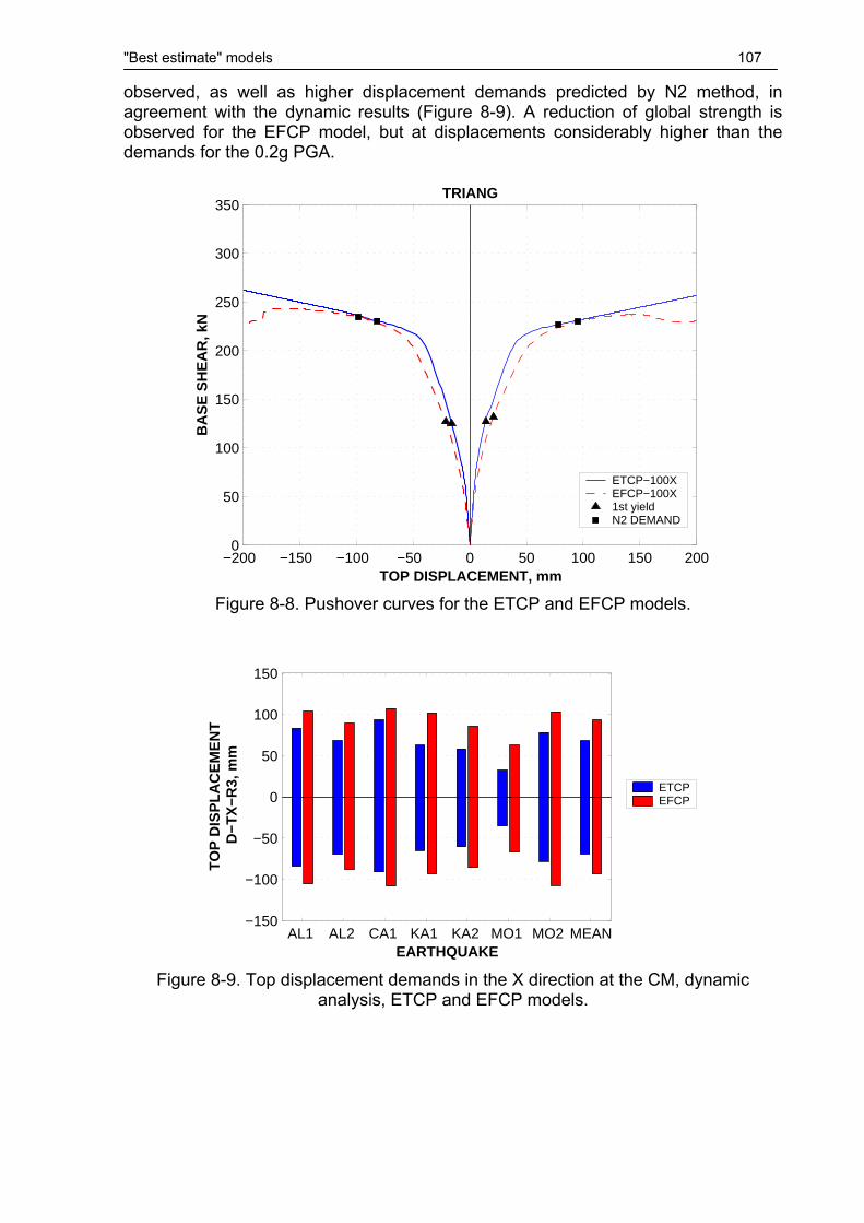
"Best estimate" models 107
observed, as well as higher displacement demands predicted by N2 method, in agreement with the dynamic results (Figure 8-9). A reduction of global strength is observed for the EFCP model, but at displacements considerably higher than the demands for the 0.2g PGA.
−200 −150 −100 −50 0 50 100 150 2000
50
100
150
200
250
300
350
TOP DISPLACEMENT, mm
BA
SE
SH
EA
R, k
NTRIANG
ETCP−100XEFCP−100X1st yieldN2 DEMAND
Figure 8-8. Pushover curves for the ETCP and EFCP models.
AL1 AL2 CA1 KA1 KA2 MO1 MO2 MEAN−150
−100
−50
0
50
100
150
EARTHQUAKE
TO
P D
ISP
LA
CE
ME
NT
D−T
X−R
3, m
m
ETCPEFCP
Figure 8-9. Top displacement demands in the X direction at the CM, dynamic
analysis, ETCP and EFCP models.

"Best estimate" models 108
−0.015−0.01−0.005 0 0.005 0.01 0.0150
2
4
6
8
10
TX, rad
HE
IGH
T, m
MEAN DYNAMIC − 0.2g − CM
ETCPEFCP
−0.015−0.01−0.005 0 0.005 0.01 0.015
0
2
4
6
8
10
TY, rad
HE
IGH
T, m
MEAN DYNAMIC − 0.2g − CM
ETCPEFCP
Figure 8-10. Interstorey drift demands, dynamic analysis, ETCP and EFCP models.
−0.015−0.01−0.005 0 0.005 0.01 0.0150
2
4
6
8
10
TX, rad
HE
IGH
T, m
N2 − SRSS − TRIANG − CM
ETCPEFCP
−0.015−0.01−0.005 0 0.005 0.01 0.015
0
2
4
6
8
10
TY, rad
HE
IGH
T, m
N2 − SRSS − TRIANG − CM
ETCPEFCP
Figure 8-11. Interstorey drift demands, pushover analysis, ETCP and EFCP models.
0 2 4 6 8 10 12 14 16 18 20 22
−100
−50
0
50
100
TIME, s
D−T
X−R
3, m
m
TOP DISPLACEMENT TH, KA1−0
ETCPEFCP
Figure 8-12. Top displacement in the X direction time history: ETCP and EFCP.
Prediction of interstorey drift demands in the X and Y direction are presented in Figure 8-10 for dynamic analyses and in Figure 8-11 for pushover analysis. The

"Best estimate" models 109
same distribution of drifts along the height is observed for the two models. Thus, higher deformation demands in the first storey are present for the X direction and in the second storey for the Y direction. The correlation of dynamic and pushover drift distribution for the X direction is different in the case of the presented TRIANG load pattern, though the demands by the pushover analysis are conservative. Improved correlation was observed for the MODE1 load pattern. Rotation demands in beams were slightly higher for the EFCP model, while shear force demands in beams and columns were similar for the two models. Top displacement time histories were generally in phase (see Figure 8-12), with higher amplitudes in the case of EFCP model. For the 0.2g PGA intensity level, global response of the ETCP and EFCP models is similar, with the exception of higher deformability of the fibre model which causes higher displacement demands. The effect of considering M-M-N interaction (EFCP model) showed little influence on the prediction of global displacement demands, due to relatively low strength degradation as a result of expected material characteristics.

Summary and Conclusions 110
9. SUMMARY AND CONCLUSIONS
Seismic response of engineering structures is characterised by considerable scatter due to variability of ground motion input. Additional uncertainties arise due to analysis procedures and modelling assumptions. Influence of the latter aspects on structural response of 3D r.c. structures was addressed in this study. Emphasis was made on simple evaluation and modelling options, applied to a torsionally unbalanced GLD r.c. frame structure characteristic for older construction in Southern Europe. Two analysis procedures were employed: nonlinear dynamic under a set of seven recorded bidirectional ground motions, and a simplified procedure (N2 method) based on nonlinear static analysis. The angle of incidence of the seismic input showed important variation in the structural response. It is an open question whether the same earthquake record applied at different incidence angles should be considered the same event or independent events (i.e. if the maximum or mean of several analyses runs is to be used in evaluation). A correlation was found though between pairs of seismic inputs applied at 180° angle difference in terms of translational and torsional response, suggesting that these should be considered the same seismic event. Strength asymmetry in one of the directions of the investigated structure caused unsymmetrical displacement demands. It is believed that a differentiation is appropriate in such cases for the positive and negative response quantities. The maximum response quantities could be obtained separately for the positive and negative senses as the maximum of two analyses runs at seismic input angles of 0° and 180°. Unidirectional and bidirectional nonlinear dynamic analyses were performed to investigate the torsional response of the structure, and whether the bidirectional response could be inferred from two unidirectional analyses (useful for simplified procedures like N2). For unidirectional seismic input translational top displacements at the stiff and flexible edges were generally in phase with top twists, though maximum translational and torsional demands did not occur generally at the same time. Irrespective of the structural model, twists were always higher for bidirectional seismic input, due to yielding of perpendicular planes of resistance that reduces torsional stiffness of the structure. However, displacement demands in a given direction under a bidirectional seismic input were dictated by the unidirectional response in the relevant direction, but could either increase or decrease in comparison with unidirectional input, depending on ground motion characteristics. If M-M-N interaction is considered in the structural model for columns, bidirectional displacement demands were higher than the unidirectional ones, due to stiffness and strength degradation of biaxially loaded columns. The SRSS combination of unidirectional response quantities showed very poor correlation with bidirectional response in the nonlinear range. Accuracy of the N2 method to predict seismic response of 3D structures is mainly related to the accuracy of 3D pushover analysis to predict the "exact" dynamic response. Two aspects related to this problem were considered in this study. The first one was investigation of load patterns containing torsional components, based on modal shape. Improved correlation was observed in several cases, but results were dependent on the structural model, and did not provide good agreement with dynamic analyses generally. Second aspect was related to prediction of structural response under bidirectional input by pushover analysis. Additionally to the SRSS combination of two separate runs in each of the two orthogonal directions, single analysis under a "bidirectional" load pattern was investigated. Bidirectional load

Summary and Conclusions 111
patterns were formed as an extension of the 100/30 rule by applying 100% of the load pattern in the direction of analysis and 30% in the orthogonal direction. The SRSS combination and bidirectional pushover analyses showed generally similar results, with slightly more conservative estimates and better agreement with dynamic analyses in the case of bidirectional load patterns. Pushover with 100/30 load patterns has the advantage of being physically more correct in the inelastic range of response, and is able of providing additional insight into the torsional response of the structure. Based on the present case study, prediction of displacement demands by the N2 method using 100/30 load patterns formed of planar load vectors seems to be a promising option, representing a good combination of simplicity, conservatism, and accuracy, when compared to the bidirectional dynamic analysis. On the side of uncertainties in structural modelling and evaluation, the following issues were addressed: rigid offsets vs. centreline dimensions of elements, bilinear, trilinear, and multilnear moment-rotation element modelling, pinching of hysteresis loops, amount of post-yielding stiffness, beam effective width, account for M-M-N interaction and strength degradation, expected vs. characteristic material strength, and evaluation of shear strength of members and joints. Analytical bilinear (secant stiffness to yield point) vs. trilinear element modelling showed important differences in the structural response (displacement demands and interstorey drift distributions). Several facts were responsible for this, including slight difference between the yield rotations of the two models and relatively low inelastic demands. Additionally, the bilinear model showed to be not well suited for unsymmetrical cross-sections, such as beams in GLD frames, leading to earlier yielding under positive moments. On the other hand, bilinear model using code-specified cracked stiffness showed a very good agreement with the trilinear model, as the code stiffness approximated by "equal area" approach the trilinear element modelling. Consideration of rigid offsets as an alternative to the centreline dimensions of elements led to important changes in global structural strength and stiffness, as well as change of relative storey shear strengths. Thus, beside higher displacement demands of the centreline model, there was a significant change in distribution of interstorey drift demands along the height of the structure. This effect was however reduced in the Y direction due to the levelling effect of the strong column. Higher demands in brittle components (element shear forces) were another consequence of rigid offsets. Large variations in post-yielding element stiffness showed little influence on the displacement demands and interstorey drift distributions. The only significant effect of higher post-yielding stiffness was the increase of elastic shear demands in elements. Modelling of pinching behaviour of elements also showed little influence on the global structural response. This is related to the particular model of pinching used in this study. Pinching behaviour is triggered after first element yielding. For most of earthquake records considered here relatively few full load reversals occurred, and displacement amplitudes generally decreased after first yielding. Therefore, maximum displacement demands were practically unaffected by the pinching behaviour. Large variations of beam effective widths were predicted by different sources. The main consequence of larger beam effective widths is higher moment capacity and reduction of ductility under negative bending (tension in top reinforcement). The global structural response was however insignificantly affected by different effective width assumptions, as the element hierarchy was basically unaffected. However,

Summary and Conclusions 112
beam effective width may be an important parameter to consider in the case of column strengthening as a rehabilitation measure. M-M-N interaction was shown to affect the response of columns when they represent the weak links in the structure leading to strength and stiffness degradation. Though global structural response was not seriously affected by consideration of biaxial moment and axial force interaction, higher interstorey drifts were observed in lower stories due to higher axial forces in columns. When modelling of element strength degradation is included in analysis, a marked increase of interstorey drift demands in lower storey subjected to higher axial forces was observed. Strength degradation seems to be an important parameter for determination of damage distribution throughout the structure and prediction of structural failure. Empirical estimates of expected material strength affect unequally the characteristic strength of steel and concrete. Due to higher concrete strength relative to steel yield strength, the column rotation capacity was improved, as concrete spalling and crushing was postponed, leading to less strength degradation. Global structural response improved accordingly, with less damage concentration in lower storey. Due to the importance of column behaviour on the global response of the SPEAR structure, two available experimental tests on columns with characteristics close to the one in the studied structure were compared with analytical predictions. Adequate performance of the bilinear and trilinear one-component models with Takeda hysteresis rules were observed prior to initiation of strength degradation. Behaviour of lumped plasticity models (one-component and multispring) was strongly dependent on the plastic hinge length, and showed poor agreement with the two experimental tests at high displacement demands. The distributed plasticity fibre model was the best in predicting cyclic behaviour of the investigated columns, including failure. Based on these findings, two additional structural models were considered, a "lower-bound" one-component with trilinear moment-rotations idealisations for both beams and columns, and an "upper-bound" one, with fibre models for columns. The two models showed similar interstorey drift distributions, but higher displacement demands for the more flexible fibre model. Evaluation of element and joint shear strength showed important variation according to different sources. However, even considering the more conservative estimates, these brittle failure modes do not exceed the imposed demands. The N2 method based on pushover analysis generally yielded conservative estimates of demands, showing a high potential for a quick estimation of seismic response of r.c. frames. The observed drawbacks of this evaluation method are related to failure to predict unsymmetrical displacement demands due to strength asymmetry, as well as the effects due to cyclic strength and stiffness degradation, in contrast to the nonlinear dynamic analysis. The "bidirectional" load patterns showed promising results and deserve further investigation. Structural models considered in this study were based on assumptions commonly adopted by engineering profession for evaluation of seismic performance of r.c. structures. Adoption of one modelling parameter or another is often based on personal experience, engineering judgement, and available computer codes, and is consequently largely subjective. Some of the modelling assumptions were shown not to influence significantly the results of analyses. However, the importance of each modelling parameters may change for different structural designs. Large scatter of both structural properties (global stiffness and strength, and local capacities such as joint shear resistance and element shear strength) and obtained demands were

Summary and Conclusions 113
observed for the range of considered models. Damage distribution through the structure was strongly affected by some parameters (such as strength degradation). Experimental validation of the different approaches is expected to have an important contribution to the development of analytical procedures for seismic assessment of engineering structures. Much work is still needed, however.

114
ACKNOWLEDGEMENTS
The work presented in this report was performed by Aurel Stratan under the supervision of Peter Fajfar. Aurel Stratan is a Ph.D. student at the Politehnica University of Timisoara, Romania, who spent ten and a half months as a visiting researcher at the University of Ljubljana, Slovenia, within the SAFERR research training network funded by the European Comission (Safety Assessment for Seismic Risk Reduction, HPRN-CT-1999-00035). The work is related also to the SPEAR project (Seismic Performance Assessment and Rehabilitation, G6RD-CT-2001-00525).

115
REFERENCES
ACI 318, (1995) "Building Code Requirements for Structural Concrete", American Concrete Institute. Alsiwat, J.M., and Saatcioglu, M., (1992) "Reinforcement anchorage slip under monotonic loading", Journal of structural engineering, Vol.118, No.9 Ambraseys, N., Smit, P., Berardi, R., Rinaldis, D., Cotton, F., and Berge-Thierry, C., (2000) "Dissemination of European Strong-Motion Data", CD-ROM Collection. European Council, Environment and Climate Research Programme. Atalay, M.B. and Penzien, J., (1975) "The Seismic Behavior of Critical Regions of Reinforced Concrete Components as Influenced by Moment, Shear and Axial Force," Report No. EERC 75-19, University of California, Berkeley. Aycardi, L., Mander, J.B., Reinhorn, A.M., (1994) "Seismic Resistance of Reinforced Concrete Frame Structures Designed Only for Gravity Loads: Experimental Performance of Subassemblages", ACI Structural Journal, V.91, No.5, 552-563. Database on column tests, University of Washington. (n.d.) Retrieved March 15, 2002, from http://maximus.ce.washington.edu/~peera1/ Calvi, G.M., Magenes, G., and Pampanin, S., (2002) "Relevance of Beam-Column Joint Damage and Collapse in RC Frame Assessment", Journal of Earthquake Engineering, Vol. 6, special issue No.1, 75-100. Cosenza, E., Manfredi, G., and Verderame, G.M., (2002) "Seismic Assessment of Gravity Load Designed R.C. Frames: Critical Issues in Structural Modelling", Journal of Earthquake Engineering, Vol. 6, special issue No.1, 101-122 Dolsek, M. and Fajfar, P. (2002) "Mathematical modelling of an infilled RC frame structure based on the results of pseudo-dynamic tests", Earthquake Engineering and Structural Dynamics, 31: 1215-1230. Eurocode 2, (2001) "Design of concrete structures", European Committee for Standardisation (CEN), final draft. Eurocode 8, (2002) "Design provisions for earthquake resistance of structures", European Committee for Standardisation (CEN), Draft No.5. Fajfar, P., (2000). "A nonlinear analysis method for performance-based seismic design". Earthquake Spectra 2000, 16(3): 573-92. Fajfar, P., Marusic, D., Perus, P., (2000) "Influence of Building Asymmetry on the Seismic Response of Structures", Chapter 7.4 in: "Moment Resistant Connections of Steel Frames in Seismic Areas", Mazzolani, F.M., (ed.), E&FN Spon, London. Fajfar, P., (2002). "Extension of the N2 method to asymmetric buildings – theoretical background". Proc. of Slovenia – Japan Workshops on Performance Based Seismic Design Methodologies, Ljubljana, Slovenia, March 2002. Fardis, M.N, (2002) "Design of an Irregular Building for the SPEAR Project". FEMA 356, (2000) "Prestandard and commentary for the seismic rehabilitation of buildings", Federal Emergency Management Agency, Washington (DC). Filippou, F.C., D'Ambrisi, A., Issa, A., (1992) "Nonlinear static and dynamic analysis of reinforced concrete subassemblages", Report No. UCB/EERC–92/08, Earthquake Engineering Research Center, University of California, Berkeley.

116
Hakuto, S., Park, R., and Tanaka, H., (1999) "Effect of Deterioration of Bond of Beam Bars Passing through Interior Beam-Column Joints on Flexural Strength and Ductility", ACI Structural Journal, V.96, No.5, 858-864. Hakuto, S., Park, R., and Tanaka, H., (2000) "Seismic Load Tests on Interior and Exterior Beam-Column Joints with Substandard Reinforcing Details", ACI Structural Journal, V.97, No.1, 11-25. Kitayama, K., Otani, S., Aoyama, H., (1991) "Development of Design Criteria for RC Interior Beam-Column Joints,” ACI SP-123, Design of Beam- Column Joints for Seismic Resistance, pp. 97-123. Kunnath, K., Hoffman, G., Reinhorn, A.M, and Mander, B., (1995) "Gravity-Load-Designed Reinforced Concrete Buildings – Part I: Seismic Evaluation of Existing Construction", ACI Structural Journal, V.92, No.3, 343-354. Li, K., (2002) "CANNY 99: 3-Dimensional nonlinear static/dynamic structural analysis computer program". Technical manual and User manual. Mander, J.B., Priestley, M.J.N, and Park., R., (1988) "Theoretical Stress-Strain Model for Confined Concrete", Journal of Structural Engineering, Vol. 114, No. 8: 1804-1825. Mehanny, S.S.F., Kuramoto, H., and Deierlein, G.G., (2001) "Stiffness Modeling of Reinforced Concrete Beam-Columns for Frame Analysis", ACI Structural Journal, V.98, No.2, 215-225. Pamapanin, S., Calvi, G.M., Moratti, M., (2001) "Seismic response of reinforced concrete beam-column joints designed for gravity load", submitted for publication to ASCE Journal of Structural Engineering. Park, R., (2002) "A Summary of Results of Simulated Seismic Load Tests on Reinforced Concrete Beam-Column Joints, Beams and Columns with Substandard Reinforcing Details", Journal of Earthquake Engineering, Vol. 6, No.2, 147-174 Paulay, T. and Priestley, M.J.N., (1992) "Seismic Design of Reinforced Concrete and Masonry Buildings", John Wiley & Sons, Inc., New York. Penelis G.G. and Kappos A.J. (1997). "Earthquake-Resistant Concrete Structures". E&FN SPON. Priestley, M.J.N., Verma, R., and Xiao, Y., (1994) "Seismic Shear Strength Demand of Reinforced Concrete Columns", Journal of Structural Engineering, Vol. 120, No.8, 2310-2329. Priestley, M.J.N., (1997) "Displacement-Based Seismic Assessment of Reinforced Concrete Buildings", Journal of Earthquake Engineering, Vol. 1, No.1, 157-192 Saatcioglu, M., Alsiwat, J.M., and Ozcebe, G., (1992) "Hysteretic behaviour of reinforcement slip in R/C members", Journal of structural engineering, Vol.118, No.9

Description of the SPEAR structure 117
Annex I. Description of the SPEAR structure
UNIVERSITY OF PATRASSTRUCTURES LABORATORY
1
Description of the 3-storey structure
The structure is a simplification of an actual 3-storey building representative of older construction in Greece, without engineered earthquake resistance. It has been designed for gravity loads alone, using the concrete design code applying in Greece between 1954 and 1995, with the construction practice and materials used in Greece in the early 70’s. The structural configuration is also typical of non-earthquake-resistant construction of that period.
The storey height is 3.0m, from top to top of the slab (net storey height 2.50m under beams). The plan of the framing and the cross-sectional dimensions of members (in cms) are given in the preceding drawings. The slab thickness is 150mm.
At present time the concrete can be considered to have fc=25MPa. The reinforcement consists of smooth bars and assumed to have as fy the nominal yield strength (320MPa).
Design gravity loads on slabs are 0.5kN/m2 for finishings and 2kN/m2 for live loads.
The reinforcement of the various structural elements is given below.
Slabs: 8mm bars at 200mm centres, both ways (or equivalent welded wire mesh)
Beam Longitudinal Reinforcement Top bars (“montage”): Two 12mm diameter bars, anchored with 180° hook at far end of column,
w/o downward bent. Bottom bars:
1. Two bars (three in Beam 4) continue straight to the supports, where they are anchored w/
180° hook at far end of column. 2. Two (or 3 in Beam 7 or 4 in Beam 4) bars are bent up towards the supports, at locations
indicated in the drawings; their bent-up ends are bent down at the far end of exterior
columns and anchored w/ 180° hook at the level of the beam soffit; over interior columns
they continue straight into next span, anchored at the top flange w/ 180° hook as indicated in the drawings.
Added top bars in Beams 9 and 10 over support at column C3: Two 20mm diameter bars are
added at top over C3, bent-down at 45° towards the span very close to the face of C3 and
anchored at beam bottom w/ 180° hooks as indicated in the drawings.
Beam stirrups8mm diameter bars at 200mm centers, closed at top w/ 90° hooks, as indicated in the drawings.
Stirrups do not continue in the joints.
Column Vertical Reinforcement and Stirrups 1. 12mm bars, as indicated in the drawings, within 8mm diameter stirrups at 250mm centers,
closed w 90° hooks. 2. Clear cover of stirrups: 15mm 3. Stirrups do not continue in the joints. 4. Vertical bars are lap spliced over 400mm at floor level, including the 1st storey (w/ starter
bars); spliced bars have 180° hooks.

Description of the SPEAR structure 118
UNIVERSITY OF PATRASSTRUCTURES LABORATORY
2
3.0 5.0
5.5
5.0
6.0
4.0
1.0
1.70
COLUMNS C1-C5 & C7-C9
0,2
5
0,25
STIRRUPS �8/25
4�12 10�12
STIRRUPS �8/25
COLUMN C6
0,25
0,7
5

Description of the SPEAR structure 119
UN
IVER
SITY
OF
PATR
ASST
RU
CTU
RES
LAB
OR
ATO
RY
4
BE
AM
1
0,2
50
,25
3
C5
C1
2�
12 (
MO
NT
AG
E)
2�
12
�8
/0.2
0
5
0,2
5
�8/0
.20
2�
12 (
MO
NT
AG
E)
2�
12C2
0,2
5
BE
AM
2
�12
�12
�12
�12

Description of the SPEAR structure 120
UN
IVER
SITY
OF
PATR
ASST
RU
CTU
RES
LAB
OR
ATO
RY
5
3
BE
AM
3
2�
12
(M
ON
TA
GE
)9
0,2
5
2�
12
0,2
5
�8/0
.20
�12
�12
BE
AM
9

Description of the SPEAR structure 121
UN
IVER
SITY
OF
PATR
ASST
RU
CTU
RES
LAB
OR
ATO
RY
6
6
0,2
5
BE
AM
4
0,2
5
3C
4
3�
20
2�
12
(MO
NT
AG
E)
�8
/0.2
0�
8/0
.20
�20
�20
�20
�20
BE
AM
7
BE
AM
5
3
0,2
50
,25
C8
C6
2�
12
(M
ON
TA
GE
)
2�
12
�8
/0.2
0�
12
�12

Description of the SPEAR structure 122
UN
IVER
SITY
OF
PATR
AS
STR
UC
TUR
ES L
ABO
RAT
OR
Y
7
6
0,2
5
BE
AM
6
0,2
5
C6
C7
2�
12
2�
12
(MO
NT
AG
E)
�8/0
.20
�12
�1
2
6
0,2
5
BE
AM
7
0,2
5
C2
2�
20
2�
12
(M
ON
TA
GE
)
�8
/0.2
0�
20
�2
0�
20
BE
AM
4

Description of the SPEAR structure 123
UN
IVER
SITY
OF
PATR
AS
STR
UC
TUR
ES L
ABO
RAT
OR
Y
8
4
BE
AM
8
C4
C7
2�
12
2�
12 (
MO
NT
AG
E)
�8
/0.2
0�
12
�12
6
0,2
50
,25
BE
AM
9
C1
2�
20
2�
12
(M
ON
TA
GE
)
�8/0
.20
�8/0
.20
2�
20
4,2
5
�8
/0.2
0
2�
12
0,7
5
2�
12
(M
ON
TA
GE
)C
3
BE
AM
10
C6
�20
�20
�1
2�
12
BE
AM
3

Description of the SPEAR structure 124
UN
IVER
SITY
OF
PATR
AS
STR
UC
TUR
ES L
ABO
RAT
OR
Y
9
BE
AM
11
5,5
0,2
50,2
5
C5
C9
2�
12
2�
12
(M
ON
TA
GE
)
�8
/0.2
0
5
�8/0
.20
2�
12
(MO
NT
AG
E)
2�
12
0,2
5
BE
AM
12
C8
�12
�1
2�
12
�1
2

Description of the SPEAR structure 125
UN
IVER
SITY
OF
PATR
AS
STR
UC
TUR
ES L
ABO
RAT
OR
Y
10
S1
15
S2
15
S5
15
S3
15
S4
15
�8
/20
�8
/10
�8/4
0
�8/40
�8/20
�8/20
�8/40
�8
/20
�8/40
�8/40
�8
/40
�8
/20
�8/2
0
�8/40
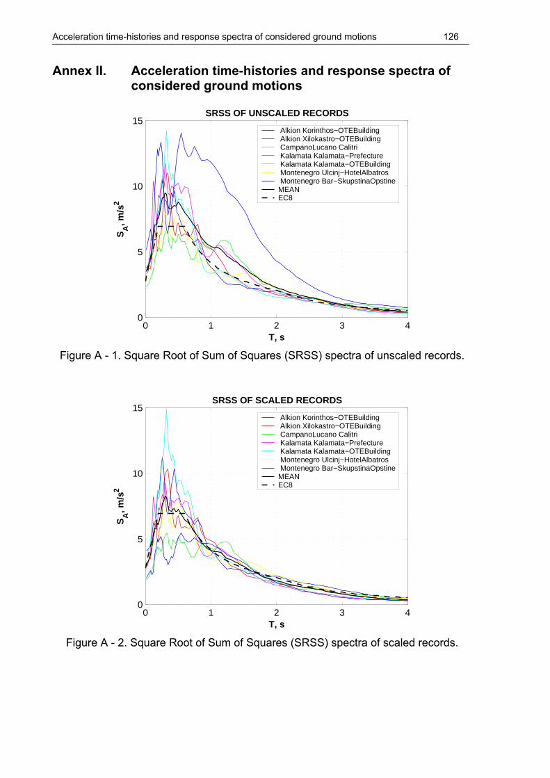
Acceleration time-histories and response spectra of considered ground motions 126
Annex II. Acceleration time-histories and response spectra of considered ground motions
0 1 2 3 40
5
10
15
T, s
SA
, m/s
2SRSS OF UNSCALED RECORDS
Alkion Korinthos−OTEBuilding Alkion Xilokastro−OTEBuilding CampanoLucano Calitri Kalamata Kalamata−Prefecture Kalamata Kalamata−OTEBuilding Montenegro Ulcinj−HotelAlbatros Montenegro Bar−SkupstinaOpstineMEANEC8
Figure A - 1. Square Root of Sum of Squares (SRSS) spectra of unscaled records.
0 1 2 3 40
5
10
15
T, s
SA
, m/s
2
SRSS OF SCALED RECORDS
Alkion Korinthos−OTEBuilding Alkion Xilokastro−OTEBuilding CampanoLucano Calitri Kalamata Kalamata−Prefecture Kalamata Kalamata−OTEBuilding Montenegro Ulcinj−HotelAlbatros Montenegro Bar−SkupstinaOpstineMEANEC8
Figure A - 2. Square Root of Sum of Squares (SRSS) spectra of scaled records.

Acceleration time-histories and response spectra of considered ground motions 127
0 1 2 3 40
2
4
6
8
10
T, s
SA
, m/s
2
X COMPONENTS SCALED
Alkion Korinthos−OTEBuilding Alkion Xilokastro−OTEBuilding CampanoLucano Calitri Kalamata Kalamata−Prefecture Kalamata Kalamata−OTEBuilding Montenegro Ulcinj−HotelAlbatros Montenegro Bar−SkupstinaOpstineMEANEC8
Figure A - 3. Acceleration response spectra of scaled records (X components).
0 1 2 3 40
2
4
6
8
10
12
14
T, s
SA
, m/s
2
Y COMPONENTS SCALED
Alkion Korinthos−OTEBuilding Alkion Xilokastro−OTEBuilding CampanoLucano Calitri Kalamata Kalamata−Prefecture Kalamata Kalamata−OTEBuilding Montenegro Ulcinj−HotelAlbatros Montenegro Bar−SkupstinaOpstineMEANEC8
Figure A - 4. Acceleration response spectra of scaled records (Y components).

Acceleration time-histories and response spectra of considered ground motions 128
0 5 10 15 20 25 30 35 40 45−4
−2
0
2
4
2.42
−2.17
TIME, s
X C
OM
PO
NE
NT
, m/s
2ACCELERATION TIME HISTORY − Alkion Korinthos−OTEBuilding (AL1 )
maxmin
0 5 10 15 20 25 30 35 40 45−4
−2
0
2
43.26
−2.4
TIME, s
Y C
OM
PO
NE
NT
, m/s
2
ACCELERATION TIME HISTORY − Alkion Korinthos−OTEBuilding (AL1 )
maxmin
0 5 10 15 20 25 30 35 40−4
−2
0
2
4
2.43
−2.66
TIME, s
X C
OM
PO
NE
NT
, m/s
2
ACCELERATION TIME HISTORY − Alkion Xilokastro−OTEBuilding (AL2 )
maxmin
0 5 10 15 20 25 30 35 40−4
−2
0
2
4
1.57
−1.25
TIME, s
Y C
OM
PO
NE
NT
, m/s
2
ACCELERATION TIME HISTORY − Alkion Xilokastro−OTEBuilding (AL2 )
maxmin

Acceleration time-histories and response spectra of considered ground motions 129
0 10 20 30 40 50 60 70 80 90−4
−2
0
2
4
1.06
−1.24
TIME, s
X C
OM
PO
NE
NT
, m/s
2
ACCELERATION TIME HISTORY − CampanoLucano Calitri (CA1 )
maxmin
0 10 20 30 40 50 60 70 80 90−4
−2
0
2
4
1.13
−1.4
TIME, s
Y C
OM
PO
NE
NT
, m/s
2
ACCELERATION TIME HISTORY − CampanoLucano Calitri (CA1 )
maxmin
0 5 10 15 20 25 30−4
−2
0
2
4
1.66
−1.67
TIME, s
X C
OM
PO
NE
NT
, m/s
2
ACCELERATION TIME HISTORY − Kalamata Kalamata−Prefecture (KA1 )
maxmin
0 5 10 15 20 25 30−4
−2
0
2
4
1.82
−2.3
TIME, s
Y C
OM
PO
NE
NT
, m/s
2
ACCELERATION TIME HISTORY − Kalamata Kalamata−Prefecture (KA1 )
maxmin

Acceleration time-histories and response spectra of considered ground motions 130
0 5 10 15 20 25 30−4
−2
0
2
4
2.47
−2.41
TIME, s
X C
OM
PO
NE
NT
, m/s
2ACCELERATION TIME HISTORY − Kalamata Kalamata−OTEBuilding (KA2 )
maxmin
0 5 10 15 20 25 30−4
−2
0
2
4
2.36
−2.8
TIME, s
Y C
OM
PO
NE
NT
, m/s
2
ACCELERATION TIME HISTORY − Kalamata Kalamata−OTEBuilding (KA2 )
maxmin
0 5 10 15 20 25 30 35 40 45−4
−2
0
2
4
1.76
−1.67
TIME, s
X C
OM
PO
NE
NT
, m/s
2
ACCELERATION TIME HISTORY − Montenegro Ulcinj−HotelAlbatros (MO1 )
maxmin
0 5 10 15 20 25 30 35 40 45−4
−2
0
2
4
2.18
−2.04
TIME, s
Y C
OM
PO
NE
NT
, m/s
2
ACCELERATION TIME HISTORY − Montenegro Ulcinj−HotelAlbatros (MO1 )
maxmin

Acceleration time-histories and response spectra of considered ground motions 131
0 5 10 15 20 25 30 35 40 45 50−4
−2
0
2
4
1.43
−1.15
TIME, s
X C
OM
PO
NE
NT
, m/s
2
ACCELERATION TIME HISTORY − Montenegro Bar−SkupstinaOpstine (MO2 )
maxmin
0 5 10 15 20 25 30 35 40 45 50−4
−2
0
2
4
1.34
−1.38
TIME, s
Y C
OM
PO
NE
NT
, m/s
2
ACCELERATION TIME HISTORY − Montenegro Bar−SkupstinaOpstine (MO2 )
maxmin
Figure A - 5. Acceleration time-histories of horizontal components of scaled ground
motions.